Int. J. Production Economics 128 (2010) 223–234

Contents lists available at ScienceDirect

Int. J. Production Economics

0925-52

doi:10.1

n Corr

E-m

(A. Kar

journal homepage: www.elsevier.com/locate/ijpe

A dynamic process-based cost modeling approach to understandlearning effects in manufacturing

Marie-Claude Nadeau a, Ashish Kar b, Richard Roth a, Randolph Kirchain a,b,n

a Engineering Systems Division, Massachusetts Institute of Technology, 77 Massachusetts Avenue, Cambridge, MA 02139, USAb Department of Materials Science and Engineering, Massachusetts Institute of Technology, 77 Massachusetts Avenue, Cambridge, MA 02139, USA

a r t i c l e i n f o

Article history:

Received 8 May 2009

Accepted 14 July 2010Available online 3 August 2010

Keywords:

Learning

Manufacturing

Process-based cost modeling

73/$ - see front matter & 2010 Published by

016/j.ijpe.2010.07.016

esponding author. Tel.: +1 617 253 4258; fax

ail addresses: nadeau@mit.edu (M.-C. Nadeau

), rroth@mit.edu (R. Roth), kirchain@mit.edu

a b s t r a c t

Informed technology decision-making requires a structured understanding of cost evolution over time.

A dynamic approach integrating learning curves and process-based cost modeling is introduced to

examine learning in manufacturing. The approach is applied to the case of a hydroforming process, and

quantifies the cost impacts of learning improvements in cycle time, downtime, and reject rates. A

comparison with cases of automotive assembly and wire drawing illustrates that variation in learning is

tied to the individual process cost structure. The results show aggregate cost evolution is strongly

dependent on cost structure and that major cost elements may not align with major cost improvement-

through-learning opportunities. The analyses can be used to focus intentional learning activities on

primary learning operational drivers.

& 2010 Published by Elsevier B.V.

1. Introduction

Across almost every sector of the economy, a defining featureof modern industry is operating in a context of nearly continuoustechnological change. Nevertheless, despite this context, indus-trial decision-makers must still select and implement technolo-gies – whether they are novel materials, processes, orarchitectures – even in the face of known-to-be-incompleteinformation. Further complicating the picture, the performance,including the economic performance, associated with noveltechnology options is likely to change over time. Changes canemerge due to a number of mechanisms, including, for example,economies of scale, and changes in the factor prices associatedwith the technology. Moreover evolution in performance canoccur through gains in productivity that develop over time, orthrough the learning effect. As a consequence, current informa-tion likely will not accurately reflect the future economics of atechnology, and making decisions on this current data cantherefore be misleading. This raises two critical questions fortechnology decision-makers: how can decision-makers pulltogether disparate pieces of information on the dynamics ofoperational and technological performance to estimate the futureeconomics of a novel technology? Based on this estimate, whatstrategies will be most effective for driving down the costs of aparticular technology?

Elsevier B.V.

: +1 617 258 7471.

), ashish.kar@gmail.com

(R. Kirchain).

This paper presents an analytical framework that allowsdecision-makers to incorporate information about expectedtechnology evolution into their economic evaluations of technol-ogy. This is accomplished through the use of process-based costmodeling (PBCM). This modeling approach deconstructs thedeterminants of manufacturing economics. As such, PBCMprovides a convenient and powerful framework within which tostudy the impact of learning on major underlying cost drivers and,therefore, on an overall cost evolution. In particular, this paperexplores the value of this approach by examining the effect oflearning in process parameters such as cycle time, downtime, andreject rate on cost evolution. This approach provides a technical-level understanding of how cost evolution depends on product orprocess characteristics. In particular, results demonstrate that thescope and timing of cost learning behavior varies across processesdepending on their technical and financial characteristics, as wellas across cost elements within individual processes. Moreover themain operational drivers of cost learning are shown to notnecessarily align with the largest cost elements. These observa-tions suggest that the proposed approach has the potential notonly to improve future cost estimates, but also to target deliberatelearning activities towards the most effective cost drivers.

The balance of this paper procedes by first presenting a reviewof past publications on the subject of learning in manufacturing. Adynamic process-based cost modeling approach to learning isthen introduced to add to this past work. The method is used inthe context of a case study on tube hydroforming, and results areexamined from the perspective of the cost impact of individualcost drivers (cycle time, downtime, and reject rate) anddifferentiated impact on various elements with the process’ cost

M.-C. Nadeau et al. / Int. J. Production Economics 128 (2010) 223–234224

structure (material, labor, energy, overhead, equipment, tooling,and building costs). These results are then compared against twoother cases, an automotive general assembly process and a copperwire drawing process, to identify differences in major costlearning drivers and the allocation of their impact on the distinctcost structures.

2. Literature review

Learning theory is based on the observation that the amount ofinput required to produce a unit output level diminishes asproduction progresses. This theory is usually attributed to T.P.Wright, who introduced a mathematical model describing alearning curve in 1936 (Wright, 1936). Wright showed that thecumulative average direct labor input for an aircraft manufacturedon a production line decreased in a predictable pattern. Thedecrease was attributed to the increased proficiency, or learning, ofthe manufacturing workers on the line as they performed variousrepetitive tasks. Wright described the learning effect using a powerfunction, where the number of labor hours required to produce asingle unit decreases with cumulative production volume.

Numerous studies in a variety of sectors and industries haveled to the recognition of the wide applicability of the learningeffect. Among other industries, the behavior has been documen-ted in the manufacturing of aircraft (Argote and Epple, 1990;Hartley, 1965), automobiles, apparel, large musical instruments(Baloff, 1971), metal products (Dudley, 1972), steam turbinegenerators (Sultan, 1974), chemicals (Lieberman, 1984; Sinclairet al., 2000), radar equipment (Preston and Keachie, 1964), ships(Argote et al., 1990), and rayon (Jarmin, 1994). Learning curveshave also been applied to the cost of power plants (Zimmerman,1982) and in the construction industry (Tan and Elias, 2000).Some recent areas of application include the semiconductorindustry (Chung, 2001; Dick, 1991; Grochowski and Hoyt,1996; Gruber, 1992; Hatch and Mowery, 1998), fuel cells(Tsuchiya and Kobayashi, 2004), ethanol production (Goldemberget al., 2004), and carbon capture and sequestration (Riahi et al.,2004).

The learning effect has also been shown to occur for aspects ofmanufacturing other than labor time input or labor costs. BostonConsulting Group (Henderson, 1972) added a new dimension to theconcept in the late 1960s, when it demonstrated that learning curvescan also characterize administrative, capital and marketing costs. Ofparticular note to the work presented here, learning behaviors havebeen shown to occur in operational characteristics such as operationalreliability (Joskow and Rozanski, 1979), error rates (Kelsey, 1984),production yield (Chung, 2001; Terwiesch and Bohn, 2001), speed ofproduction (Alamri and Balkhi, 2007; Dar-El and Rubinovitz, 1991;Terwiesch and Bohn, 2001), and the amount of rework needed after amanufacturing process (Jaber and Guiffrida, 2008).

Although learning effects have been demonstrated in a largenumber of contexts, high variations in learning rates have alsobeen observed across different products and organizations.Gruber (1992) has shown that variations in learning occurredwithin a single semiconductor manufacturing company acrosschip types, even if the chips were considered very similar.Variations have also been observed across organizations produ-cing the same product (Argote et al., 1990; Argote and Epple,1990), and across shifts within the same organization (Epple et al.,1991). Understanding the sources of these variations, and thus theunderlying mechanisms that drive learning, has been the object ofsignificant work. The importance of understanding the underlyingmechanisms of learning is based on the observation that thelearning process is not guaranteed; rather, it is an opportunityfor management action to produce improvements (Day and

Montgomery, 1983; Dutton. and Thomas, 1984; Terwiesch andBohn, 2001). This view of the learning effect as actionable hasbeen adopted by many in the context of developing firmoperational strategies. Spence (1981), for example, developed amodel of competitive interaction and industry evolution, con-cluding that a firm can achieve higher profits in the long runby increasing current production in order to move down thelearning curve faster than its competitors. Argote has particularlyfocused on the knowledge management tools and organizationalmechanisms responsible for learning (Argote, 1993, Argote et al.,2003). Lapre et al. (2000) have shown that quality improvementactivities can positively impact learning when they lead toacquiring both know–why and know–how. Hatch and Dyer(2004) also show that investment in human capital can lead toaccelerated learning. Terwiesch and Xu (2004) have examinedhow learning effort and process change can be traded off, in orderto optimize a desired outcome. While these studies have providedpowerful insights into strategies to improve learning, they focuson high-level operational and organizational strategies and foregodiscussions of a mechanism by which different aspects of learningand operational performance improvements could be prioritizedwithin a facility. To explore the possibility of gaining that insight,this paper will couple the concepts of a learning effect within adetailed generative cost model.

Others have explored the coupling of learning and moredetailed models. Womer (1979), in particular, emphasized theimportance of integrating production functions with learningmodels, and production functions integrating a learning curveparameter have been used in a number of empirical studies(Argote et al., 1990; Preston and Keachie, 1964; Rapping, 1965). Inanother paper, Day and Montgomery (1983) characterized their‘experience curve’ as comprising the effects of learning, techno-logical advances, and scale economies on an aggregate productioncost. They also noted that different learning curves could beapplied to different cost types, among which they distinguishedvalue-added and controllable costs, and proposed that thisapproach could yield a total cost learning curve significantlydifferent from the result obtained, if a single curve is applied atthe aggregate level. Nadler and Smith (1963) developed a methodwhich decomposes a manufacturing process into multipleprocesses and applies a learning curve to the cost of operatingeach of them. The total cost learning function is then the time-weighted sum of these individual process learning curves. Mostrecently, Terwiesch and Bohn (2001) examine how learning in anoperational characteristic, yield, provides insight into the trade-off between experimentation (for the purposes of increasedlearning) and the attendant loss of production, and into howthese trade-offs depend on the prevailing economic conditions.

To date, across this literature, no study has explored thedifferentiated effects of learning across various operational char-acteristics, how those effects combine and translate into aggregatefinancial behavior, or the trade-offs that exist in emphasizingspecific elements of operational learning. This paper will demon-strate that by developing insight at the operational level, it may bepossible to both better characterize the potential for cost learningof a specific technology based on that technology’s financial andprocess characteristics, and to prioritize the efforts of an opera-tional manager to maximize the economic impact of learningactivities. The former should improve technology selection deci-sion-making; the latter should improve operational decisions.

3. The process-based cost modeling approach

The present paper characterizes the implications of learning atan operational level by mapping the effect of learning in multiple

M.-C. Nadeau et al. / Int. J. Production Economics 128 (2010) 223–234 225

process parameters on the cost of a given technology. The impactof process parameters on production cost has been characterizedin a static fashion previously through the use of a number ofgenerative costing methods. This study will extend this byintegrating learning effects into a specific modeling method,process-based cost modeling (PBCM), which analytically derivesfrom technical and operational drivers to estimate the total cost ofproduction (Kirchain and Field, 2001).

Learning theory presents a dynamic perspective on cost, whileprocess-based cost modeling provides a characterization of thestatic link between process parameters and production cost. Bycombining the two approaches, it is possible to analyze the effectof learning curves on individual process parameters and study theimpact of this learning on the dynamic evolution of totalproduction cost. To do this, a dynamic component must be addedto the traditional PBCM framework.

3.1. Static process-based cost modeling framework

The PBCM framework introduced by Field et al. (2007) isrepresented in Fig. 1. It postulates that cost can be regarded as afunction of technical factors, such as cycle time, downtime, rejectrate, equipment and tooling requirements, or the material used.These technical factors, including operational inefficiencies, drivethe quantity of factor resources that are required to produce agiven level of output for a given type of technology.Understanding the effect of these underlying technical costdrivers can provide insight for managers and engineers as towhat process improvements are most critical to lower productioncosts (Fuchs et al., 2006). It also allows them to better predictmanufacturing costs for new technologies or designs, since itincorporates knowledge of technical, often more tangible,information about the products and processes, and does not relywholly on historical data, which may not exist for noveltechnologies. Fig. 1 shows the break-down of the overall costmodel into three interconnected sub-models that describe theprocess, operational, and financial aspects of production.

The process model is based on engineering, technological andscientific principles. It relates final product or part characteristicssuch as size, shape, and material to the technical parameters ofthe process required to produce that product. These parameterscan include cycle time (the total processing time required for asingle part); equipment capacity, such as press tonnage and size;and tooling requirements. The process model also characterizesthe relationships and constraints between various processingvariables. For example, increases in downtime and reject rates canlimit the technical feasibility of reductions in cycle time.

Processing requirements are passed on to the operational sub-model along with production operating conditions, which takeinto account the production shift schedule, working hours, andproduction volume. These inputs are translated into the totalamount of equipment, labor, floor space, energy, and otherresources needed to achieve the desired product output.

The financial sub-model applies factor prices to the resourcerequirements determined by the operations model, and allocatescosts over time and across products in order to output a unitproduction cost. This figure can be broken down in terms of fixed

Production Cost

$

Annual Prod. Volume

ProcessModel

OperationsModel

FinancialModel

Prod

uct

Des

crip

tion

Proc

essi

ngR

equi

rem

ents

Operating Conditions Factor Prices

Res

ourc

eR

equi

rem

ents

Fig. 1. Process-based cost modeling framework (Field et al., 2007).

and variable costs or into individual contributions from labor,equipment, tooling, and material costs. Although this cost is nottime-dependent or cumulative volume-dependent, the underlyingrelationships implemented by the model enable the analysis ofvariations in production costs as operating and processingparameters change. Such sensitivity analyses allow identificationof primary cost drivers that can be targeted for improvement.

3.2. Description of the static PBCM

Production costs reported for the case studies presented hereare the result of a simple process-based cost model. DetailedPBCMs have been developed to inform technology selectionacross a number of applications ranging from automobilestructures (Han and Clark, 1995; Johnson and Kirchain, 2009) tomicrophotonic components (Singer and Wzorek, 1997) to electro-nics disposal (Gregory and Kirchain, 2006). For this research, theauthors specifically chose to apply a simple model which,although broad in scope (covering seven cost elements), compre-hends only basic common operational considerations for parallel-scaled processes. Of particular note, the authors have assumedthat the key operational characteristics are independent andknown (deterministic). Several authors have pointed out that thisdoes not always hold and can impact decision-making. Key workin this space has demonstrated that aspects of operationalperformance, including both production rate and downtime, arein fact variable and that this variability alters optimal decision-making. For example, Yano and Lee (1995) and more recentlyMula et al. (2006) review the extensive range of work on the effectof production uncertainty on various operations managementdecisions. In a related set of work, several authors have pointedout that it can be important to consider the interdependence ofoperational performance (e.g., reject rates and downtimes) onoperational decisions, such as task routing (Cao et al., 2009), lotsize (Darwish, 2008; Jaber et al., 2009; Porteus, 1986; Urban,1998; Yano and Lee, 1995), and line running rate (Bohn andTerwiesch, 1999; Jaikumar and Bohn, 1992; Terwiesch and Bohn,2001), particularly when these are stochastic in nature.

Although these effects are real and can be important, they areomitted in the model presented subsequently. The authors believethat employing a simple deterministic model makes it easier tofocus the discussion on the implications of considering thedynamics of learning. Most importantly, the authors believe thatmore sophisticated consideration of parametric interdependenceor uncertainty would not materially alter the observationsreported in this paper. Where appropriate, this is discussed inmore detail subsequently. Finally, it is worth emphasizing that themodel structure presented in this section is intended to representa static cost model. The next section discusses how parameters inthis model change to capture the time-dependent effects oflearning.

First, each product is assumed to be produced through aprocess, each completed in cycle time CT. For simplicity, we modelthe process as if it comprised only a single step. Given thissimplification, it is possible to derive the gross number of partsproduced, Vgross, from the overall target net volume, Vnet, and thereject rate, rej, for the process. Specifically, the gross number ofparts, Vgross, produced is

Vgross ¼Vnet

1�rejð1Þ

It is assumed that all parts that are rejected are not salable totheir intended market, but may be resold for scrap (see Eq. (7)).The implications of any rework costs and revenues are accountedfor only implicitly through the scrap price (the firm thatpurchases rejects parts for scrap, may elect to rework those

M.-C. Nadeau et al. / Int. J. Production Economics 128 (2010) 223–234226

parts), but are not explicitly modeled. By an extension, the totaloperating time, t, required in a year for the production of Vnet

defect-free parts is simply:

t¼ CT � Vgross ð2Þ

The operating time, or uptime, of a production line isconsidered to be 24 h per day on days when the plant is open,less the time when the line is either idle due to lack of demand orunavailable for production

UT ¼DPY � ð24�NS�UD�PB�UBÞ�Idle ð3Þ

where UT is the line uptime per year; DPY is the number of days ofplant operation per year; NS is the amount of time per day whenno shifts are run; UD represents unplanned downtime andbreakdowns; PB is the time for paid breaks; UB is time for unpaidbreaks; and Idle is the time during the year when the plant isavailable but not running, for example due to lack of demand.Given the uptime of a single line and the operating timerequirements to produce a target volume, the integer number ofproduction lines (nl) needed is

nl¼t

UT

l mð4Þ

Notably, several authors have found that learning progressesat a slower rate, when production is distributed across multiplelines (i.e., nl41), facilities (Darr et al., 1995; Lapre and VanWassenhove, 2001), or multiple shifts (Epple et al., 1991) ascompared to an equivalent volume produced on one line. For thisreason, learning rates (see next section) determined by examiningone line should not be applied without an adaptation to situationsrequiring significant parallelization. For the empirical analysespresented subquently, cases are limited to contexts where a singleline is sufficient to meet production goals.

It is also possible to compute the annual amount of paid time(APT) required from workers in the plant, considering that theyreceive wages for paid breaks and unplanned downtime, as wellas when the plant is idle.

APT ¼Xnl

j ¼ 1

ð24�NSj�UBjÞ ð5Þ

where NSj is the amount of time per day when no shifts are run onthe jth production line and UBj is the time for unpaid breaks forworkers on line j.

The next part of the PBCM constitutes the financial model, andapplies factor prices to the resource requirements describedabove. It also allocates cost over time and production to computea unit cost per part produced. The annual costs in the modelpresented here are divided into seven categories:

Ctotal ¼ CmaterialþClaborþCoverheadþCenergyþCbuildingþCequipmentþCtooling

ð6Þ

Material cost is the product of the number of parts enteringproduction (Vgross), the weight of the part w, and the price per unitmass p. Parts rejected during processing constitute scrap, whichcan be sold at a price pscrap.

Cmaterial ¼ Vgrosswp�ðVgross�VnetÞwpscrap ð7Þ

Labor cost is the product of the paid time required to producethe target volume, and the labor wage rate pwage. Because themodel assumes that other parts or products may be produced inthe plant when it is available but not used to produce the part ofinterest. The labor time attributed to the production of this part isnot necessarily equal to the total annual paid time of the plant.Instead, this annual paid time is multiplied by the fraction of theavailable plant time (UT+ Idle) that is actually used to produce

the part.

Clabor ¼ APT � pwage �t

UTð8Þ

The overhead cost in this model is meant to capture theindirect labor required to maintain production, which is modeledusing a ratio of the number of indirect workers required for eachdirect worker (ind). Indirect workers are paid at a wage rate pind;the cost of overhead is thus

Coverhead ¼ APT � ind� pind �t

UTð9Þ

The energy cost is proportional to the average energyconsumed by the process, which is modeled as a powerrequirement E multiplied by the operating time of the process

Cenergy ¼ E� t� penergy ð10Þ

Building, tooling and equipment are considered to be capitalinvestments. In order to incorporate these investments into a unitcost, the financial model distributes them across time bydetermining a series of annual payments that are financiallyequivalent to the initial investment. The distribution is done overthe useful life of the building, equipment or tool in question, andapplies a common discount rate. The capital recovery factor CRFj

(where the index j is used to represent either building, equipment,or tooling) used to determine annual payments is therefore

CRFj ¼rð1þrÞLj

ð1þrÞLj�1ð11Þ

where r is the annual discount rate and Lj is the useful life innumber of years.

The annual building cost is computed given an initial buildingcapital investment CAPbuilding

Cbuilding ¼ CRFbuilding �t

UT� CAPbuilding ð12Þ

The equipment in the plant is assumed to be non-dedicatedand shared across other parts produced; therefore, the cost ofequipment can be multiplied by the fraction of available planttime used to produce the part of interest. Equipment capitalinvestment is the sum of the equipment capital required for eachline (CAPequipment), multiplied by the number of lines in the plant.The annual equipment cost is

Cequipment ¼Xnl

j ¼ 1

CRFequipment �t

UT� CAPequipment

� �ð13Þ

Tooling, on the other hand, is assumed to be dedicated to acertain part. The entire tooling capital investment is thereforeattributed to the part considered by the model:

Ctooling ¼Xnl

j ¼ 1

ðCRFtooling � CAPtoolingÞ ð14Þ

Finally, these annual costs can be used to compute a unit costper part (U)

Utotal ¼Ctotal

Vnetð15Þ

The production cost obtained from the PBCM can be examinedin a number of different ways. Individual cost categories and sub-processes can be compared to identify primary cost drivers.Sensitivity analyses on various process parameters can also beperformed to further characterize their impact on system and costbehavior. A detailed level of sensitivity analysis is possiblebecause the model derives cost from technical informationdefined at the process level, rather than using statistical methodsto determine cost directly from the part description. This makes ita powerful tool to understand the effects and interactions of thedifferent technical parameters that impact manufacturing cost.

Production Cost

$ProcessModel

OperationsModel

FinancialModelPr

oduc

t D

escr

iptio

nOperatingConditions

FactorPrices

Res

ourc

eR

equi

rem

ents

ProcessingRequirements

Cum. Vol.

Cyc

le T

ime

Cum. Vol.

Dow

ntim

e

Cum. Vol.

Rej

ect r

ate Cumulative

Prod. Volume

Fig. 2. Dynamic process-based cost modeling framework.

M.-C. Nadeau et al. / Int. J. Production Economics 128 (2010) 223–234 227

4. Modeling learning: a dynamic process-based cost model

The process-based cost model described above provides a costfigure, which is static, representing a snapshot in time of a particularset of process parameters. In this section, a method will bepresented for expanding the use of PBCMs to address the questionof cost evolution with time, and particularly through learning.

4.1. Dynamic PBCM framework

Because the PBCM considers a number of technical or processparameters in its cost calculation, it is possible to investigatethe specific impact on cost if these vary over time through amechanism, such as the learning effect. In the frameworkpresented here and illustrated in Fig. 2, this effect isincorporated by applying a learning curve to certain processingrequirements such that they, as well as the resulting cost,effectively vary as production progresses.

The parameters chosen here to investigate learning effects arecycle time (CT), unplanned downtime or breakdowns (UD), andthe reject rate (rej), each of which become functions of thecumulative number of components produced until given time (Vt)and, therefore, of time(t)–CT(Vt)

1, UD(Vt), and rej(Vt) and CT(t),UD(t), and rej(t), respectively. These parameters are not meantto represent an exhaustive list of the operational characteristicsthat are or could be impacted by learning. Rather, they representexamples of such characteristics, chosen in the interest offocusing and simplifying the analysis. Furthermore, learningeffects have been observed in the previous literature foroperational variables, which are either equivalent or comparablein nature to those explored herein, such as speed of production(Terwiesch and Bohn, 2001), operational reliability (Joskow andRozanski, 1979), and yield (Chung, 2001; Jaber and Khan 2010).Finally, for the case explored subsequently, these representparameters for which the data collected show distinct improve-ment over time.

As was pointed out previously, cycle time can be anoperational decision, and then may influence other elements ofprocess performance, including both reject rate and unplanneddowntime (Bohn and Terwiesch, 1999). In a real world context,the cycle time employed for a specific process should be selectedin light of these issues. In the analyses presented subsequently,we implicitly assume that cycle time is selected exogenouslythrough some rational means (e.g., as described by Terwiesch andBohn (2001)). In cases where empirical data on all or most criticaloperational characteristics is not available, it may be important to

1 As functions of cumulative volume and time, these parameters feed directly

back into the static model as presented in the previous section. In the interest of

brevity, the mathematical description is not repeated here in a time-dependent

form, but the consequence is that most cost elements become time-dependent.

elaborate on the model described herein to make this decisionendogenous.

4.2. Learning curve functional form

The functional form of the learning curve has been widelydebated. However, Wright’s learning model, which consists of alog–linear curve varying with cumulative volume, is by far themost commonly used (for examples of its application, see Argoteand Epple (1990); Henderson (1972); Lieberman (1987); Riahiet al. (2004)). Other learning curve geometries have been appliedand discussed in the literature, and were reviewed by Yelle (1979)and more recently by Jaber (2006). Issues that have been raisedwith the log–linear model include overestimation of earlylearning gains (Baloff, 1971; Jaber et al., 2008) and saturation oflearning that can occur over time, which are sometimes observedin the learning behavior (Baloff, 1971; De Jong, 1957; Jaber et al.,2008) as well as several others discussed in Jaber (2006).Saturation, or plateauing, of learning is widely noted in theliterature, and has been postulated to derive from a lack of capitalinvestment (Jaber and Guiffrida, 2004), low expectations (Hirsch-mann, 1964), or knowledge depreciation and forgetting (Eppleet al., 1991). Although little empirical evidence exists to defendthese mechanisms, recent work by Jaber and Guiffrida suggeststhat the interrelationship between the rate of learning duringreworking and the rate of process deterioration could explainprocess performance plateauing (Jaber and Guiffrida, 2008; Jaberand Guiffrida, 2004). Unfortunately, much work needs to be donebefore consensus exists on the cause of plateauing (Jaber, 2006).

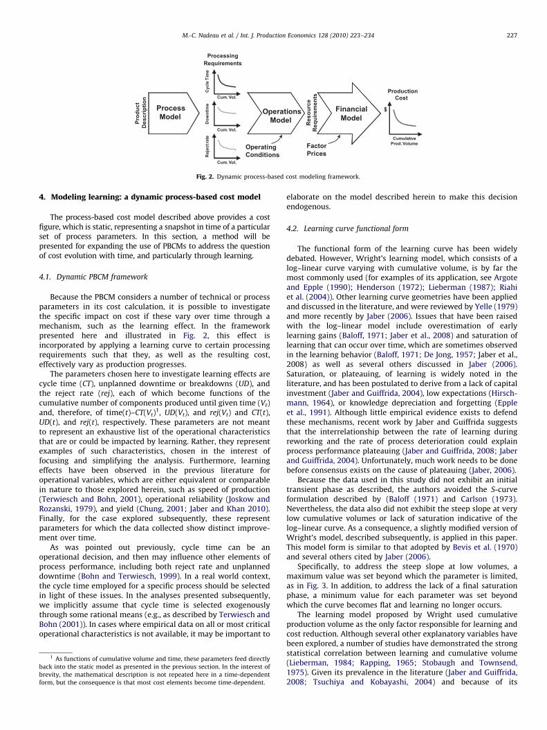
Because the data used in this study did not exhibit an initialtransient phase as described, the authors avoided the S-curveformulation described by (Baloff (1971) and Carlson (1973).Nevertheless, the data also did not exhibit the steep slope at verylow cumulative volumes or lack of saturation indicative of thelog–linear curve. As a consequence, a slightly modified version ofWright’s model, described subsequently, is applied in this paper.This model form is similar to that adopted by Bevis et al. (1970)and several others cited by Jaber (2006).

Specifically, to address the steep slope at low volumes, amaximum value was set beyond which the parameter is limited,as in Fig. 3. In addition, to address the lack of a final saturationphase, a minimum value for each parameter was set beyondwhich the curve becomes flat and learning no longer occurs.

The learning model proposed by Wright used cumulativeproduction volume as the only factor responsible for learning andcost reduction. Although several other explanatory variables havebeen explored, a number of studies have demonstrated the strongstatistical correlation between learning and cumulative volume(Lieberman, 1984; Rapping, 1965; Stobaugh and Townsend,1975). Given its prevalence in the literature (Jaber and Guiffrida,2008; Tsuchiya and Kobayashi, 2004) and because of its

0.0

0.2

0.4

0.6

0.8

1.0

0 200 400 600 800 1000

Proc

ess

para

met

er

Cumulative volume (thousands)

(a)

(b)

Fig. 3. (a) Log–linear curve without saturation; (b) log–linear curve with

maximum and minimum saturation levels.

M.-C. Nadeau et al. / Int. J. Production Economics 128 (2010) 223–234228

explanatory value for the data set examined subsequently,cumulative volume was used as the driver for learning behaviorin this paper.

4.3. Learning curve definition and application

Wright described the learning effect using a log–linearfunction of the form

hV ¼ aV�b ð16Þ

where hv is the number of labor hours required to produce the Vthunit; a is the number of labor hours required to produce the firstunit, hence a¼h1; V is the cumulative number of units produced;and b is a parameter describing the learning rate, i.e., the rate atwhich performance improves with respect to the cumulativeoutput.

The modified log–linear curve shown in Fig. 3(b) was appliedto the three process parameters mentioned above in order toproduce a dynamic process-based cost model that outputs cost asa function of cumulative production volume.

Parameters a and b for the log–linear portion of the learningcurve were determined via least-squares regression for Wright’smodel in the form

lnð ~Y3

tÞ ¼ lnða3Þþb3 lnðVtÞ ð17Þ

where ~Y3

t is the value of the process parameter for which learningoccurs (assuming it follows a log–linear pattern), at time t (inmonths); and Vt is the cumulative volume produced up until time t.For the purposes of the analyses in this paper, it is assumed thatlearning progresses with cumulative volume produced (i.e., asopposed to related trends such as time). To better reflect theempirical data collected for the case study, the learning behaviorwas modeled using a truncated form of the log–linear relationship.Specifically, process parameter evolution was modeled such that

Y 3

t ¼minðmaxð ~Y3

t ,Y3

minÞ,Y3

maxÞ ¼minðmaxða3V�b3

t ,Y 3

minÞ,Y3

maxÞ ð18Þ

In this model, the parameter b defines the learning rate, ortiming. A high value of b indicates fast learning with respect tocumulative volume. The values of Y3

max and Y3

min define the highestand lowest values of Yo that can be observed, respectively. For thesubsequent empirical analyses, Y 3

max and Y 3

min, were chosen to bethe maximum and minimum values observed in the data set. Theydetermine what will be referred to later as the learning scope, orthe magnitude of the improvement that can be achieved. Scopecan be defined as ðYmax�YminÞ=Ymax.

In order to explore the impact of learning in a number ofdifferent operational contexts, and to ensure that the learning

pattern was consistently maintained, the specific relationshipdescribed in (18) was normalized, and then rescaled as appro-priate. It is possible to apply the same learning pattern (as definedby a and b) to multiple process parameters, which take variousranges of values. This can be done by normalizing the learningcurve output, and then rescaling it to a different set of maximumand minimum values. For a maximum parameter value of Y 3

max

and minimum of Y 3

min, the normalized curve is defined as

Y3

t ¼Y 3

t�Y 3

min

Y 3

max�Y 3

min

ð19Þ

where Y3

t is the normalized learning curve output, with 0oY3

t o1.This normalized curve can be scaled up to represent the evolutionof a process parameter, Yx

t , using an equation of the form

Yxt ¼ Y

3

tðYxmax�Yx

minÞþYxmin ð20Þ

In the analysis that follows, empirical data were available onthe process reject rates, cycle times, and downtimes. Althoughprevious work suggests that these quantities can be interrelated,and while the authors would have preferred to construct a modelthat captured this interrelationship; the data was not available tomake this possible. Fortunately, the nature of the data collectedembeds any such interrelationship in the observed performan-ce—although it does not guarantee that an optimal cycle time wasselected. As such, while not endogenously determined, the resultsshould reflect the impact of this interdependency.

5. Learning and dynamic PBCM: the case of tubehydroforming

We present an application of the dynamic PBCM describedabove to the case study of tube hydroforming, a process that usespressurized fluid to change the cross-sectional shape of a ductilemetal tube along its length. (See Koc- (2008) for a more detaileddescription of the process and its application). First, the shape ofthe learning curve is determined for each process parameterexamined. The chosen learning patterns are then incorporated inthe PBCM, allowing the analysis of their individual and combinedimpacts on unit cost.

5.1. Learning curve parameters

Several years of monthly production data on volume, cycletime, and unplanned downtime for a tube hydroforming produc-tion line operated by a major U.S. automaker between June 1999and August 2004 were collected and used to determine learningcurve parameters. This was done via least-squares regression asdescribed above. An example of the curve fitted to cycle time datais shown in Fig. 4.

Resulting model parameters a and b for each of the two datasets (cycle time and unplanned downtime), as well as thesignificance of the F-statistic from the regression analyses againstthe explanatory variable cumulative production volume, aresummarized in Table 1. From this information, it is clear thatcumulative production volume is statistically significant as adescriptor of variation in these data.

No data were available to perform a regression on reject rateimprovement. For the purposes of this study, it was assumed thatthe reject rate parameter experienced the same learning patternas unplanned downtime after the normalization of the learningcurve. This pattern of reject rate evolution is consistent with thatobserved by Jaber and Bonney (2003).The maximum and mini-mum saturation levels used to normalize each process para-meter’s learning curve are shown in Table 2. Values for cycle timeand unplanned downtime are based on the collected data, while

Fig. 4. Log–linear regression of tube hydroforming cycle time data vs. cumulative

volume.

Table 1Summary of log–linear learning curve parameters.

Process parameter a b Significance on F-statistic

Cycle time (CT) 2.829 0.093 1.077E-6

Unplanned downtime (UD) 0.562 0.177 0.0044

Table 2Summary of process parameter maximum and minimum saturation levels.

Process parameter Ymax Ymin Scope (%)

Cycle time (CT) 1.160 0.764 34

Unplanned downtime (UD) 0.103 0.047 54

Reject rate (rej) 0.200 0.100 50

Table 3Key cost model inputs.

Key inputs Hydroform Assembly Copper wire

Production volume (units/year) 500,000 200,000 400,000

Interest rate (%/year) 12% 12% 12%

Workers per line 3 500 1

Indirect/direct worker ratio 0.2 0.5 0.2

Power consumption (kWh/line) 240 40,000 70

Part weight (kg) 2.8 – 7

Material price ($/kg) 0.65 – 3.30

Scrap price ($/kg) 0.10 – 1.00

Equipment investment ($/line) $4.5 M $15 M $1.5 M

Tooling investment ($/line) $1.7 M $75 M $1.5 M

Building area per line (m2) 2200 95,000 2500

Fig. 5. Total cost improvement through learning with an increasing cumulative

production volume, by the process parameter.

M.-C. Nadeau et al. / Int. J. Production Economics 128 (2010) 223–234 229

reject rate maximum and minimum values are assumptions basedon estimates by hydroforming process experts from the same firmat which data were collected.

The learning patterns were inserted into the simple process-based cost model, resulting in a cost figure, which varied withcumulative production volume. Other inputs to the cost modelwere chosen to reflect the tube hydroforming of a hypotheticalpart having eight bends, and weighing approximately 2.8 kg,which is illustrative of a key part typically used in an automotiveengine cradle. Key cost model inputs can be found in Table 3 inSection 6.

5.2. Dynamic PBCM results

Model output suggests that the unit cost of a hydroformed partwould experience more than a 25% reduction over a cumulativeproduction of approximately 1.25 million parts beyond thatobserved to date, when learning effects in the three processparameters mentioned above are combined. (Note that thehydroforming process was first utilized commercially in 1992and had been used outside of the firm from which production datawere collected for this study. Based on interviews with industryexperts, the authors estimate that somewhere between 0.5million and 1 million parts had been produced by mid 1999, thetimeframe of our earliest data. Based on a conventional log–linearmodel, these figures would imply a learning rate somewherebetween 0.8 and 0.85. All subsequent references to cumulativevolume represent the number of units produced beyond theearliest date for which data was available.) Because learning isapplied at the operational level in the PBCM, contributions to costimprovement from learning in individual process parameters can

be isolated as in Fig. 5. It is interesting to note that the combinedlearning effect is not simply the sum of the learning effectsfrom each of the individual parameters. While individual costsavings sum up to $6.50 over 1.25 million additional parts, thecombined learning only generates a unit cost saving of $5.74 overthe same period. The underlying relationships of the dynamicPBCM allow the user to examine this combined learning effect,while taking into account the fact that improvements do nottranslate into aggregate cost savings in a simple additive way.Looking back at the cost model, it is clear that some of theseeffects are convolved in a manner that mutes their mutual impact.For example, consider the convolved impact of cycle time (CT(t))and reject rate (rej(t)) on required operating time (t(t)), a partialdeterminant of every cost element save for materials cost.Specifically, combining Eqs. (1) and (2), we get an expression fort of the form

tðtÞ ¼ CTðtÞ � VgrossðtÞ ¼ CTðtÞVnetðtÞ

1�rejðtÞð21Þ

Based on this expression, t-derived costs would decline asCT(t) declines, but this effect would be dampened by improve-ments in rej(t) and vice versa. Similar interdependencies existbetween each of the learning parameters explored herein.

The analysis represented in Fig. 5 would indicate that, for thehydroforming process, the majority of the cost improvementcomes from learning on cycle time. This suggests that this is theoperational characteristic that managers and engineers shouldfocus on improving in order to gain maximum cost impact.

Given the way that this analysis has been structured, somemay question the normative managerial value of this result—theanalysis in Fig. 5 represents a retrospective assessment of what

Fig. 6. Cost improvement by operational parameter, for identical and differing

learning rates and scopes.

M.-C. Nadeau et al. / Int. J. Production Economics 128 (2010) 223–234230

happened in the actual execution of tube hydroforming.The specific learning rates that were observed are the result ofthe nature of the technology, the adaptability of the workforce,and whatever managerial emphasis (training, experimentation, orotherwise) was applied over that period, of which no specificknowledge is available. Fortunately, the nature of the PBCMplatform makes is trivial to explore the implications of otherlearning patterns and their consequence for overall potential costimprovements.

Specifically, to explore the generality of the above observationconcerning the importance of cycle time learning, a similaranalysis was conducted, but with all operational characteristicslearning at the maximum observed rate and maximum expert-anticipated scope. Notably, for this case study, cycle time learninghas a larger impact, despite a slower learning rate and a lowerscope of learning than the other two parameters (cf. Table 2). Assuch, this additional analysis would be expected to only reinforcethe importance of cycle time learning. Nevertheless, from amethodological perspective, it is valuable to explore the implica-tions of such an analysis.

Fig. 6 shows total cost improvement at the end of the analysisscope (here 1.25 million additional parts produced) in caseswhere learning rates and scopes either differ among operationalparameters (the baseline case, as shown in Fig. 5) or are set tomaximum expert-anticipated values across all three parameters.In the latter case, the rate was set at the fastest observed rate(b¼0.177), and the scope was set at 50% for all three operationalparameters.

Based on this analysis, the predominance of cycle time as adriver for learning in this case persists even if all parameters areaffected by the same learning rate and scope. Under thoseconditions, cycle time has the most significant impact, followedby the reject rate. This can partly be explained by the fact that, forthis process, cycle time has more influence on actual productiontime than downtime: while hydroforming downtime takes upapproximately 5–10% of the plant’s operating time, cycle timedetermines the use of approximately 90–95% of the available time.

The difference in an impact between cycle time and reject ratecan further be explained by looking at the cost structure of theprocess. While learning on reject rates typically greatly improvesmaterial costs, this cost category only constitutes a small portionof the overall cost structure for the hydroforming process (seeFig. 7). Fig. 8 shows that learning has the most impact on labor,equipment and building costs. While cycle time has a directimpact on how much labor is required, it also improves utilizationof non-dedicated resources, such as equipment and building. As

the time required to produce the desired volume is reduced, theseresources can be used for other production, and the portion oftheir cost allocated to the part of interest is reduced.

Fig. 7 also indicates that tooling is the main cost contributor forthe hydroforming process. However, because tools are defined asdedicated to a single part type, improvements in productionperformance do not affect significantly the tool cost after theirinitial purchase. Although on the margins, tooling costs could varywhen additional lines are needed, they are generally unaffectedby learning as is shown by Fig. 8. Tooling costs exhibit no unit costimprovement between cumulative volumes of zero and 1.25million additional parts produced.

In the case of tube hydroforming, the use of a dynamic PBCMidentifies equipment costs and cycle time decrease as the mainsources of cost improvement through learning. However, theseconclusions derive from the nature of the cost structure and thetechnological possibilities for an improvement in operationsand therefore are technology- and process-specific. The casespresented below will demonstrate how learning effects and theirsources can differ between processes, and how a dynamic PBCMcan be used to characterize these differences.

6. Differences in learning effects between processes andtechnologies

The cost of a hydroformed part is dominated by fixed costs,such as investments in tooling, equipment and building. Twoother cases are analyzed below to illustrate the variations inlearning effects that occur when the cost elements for atechnology are distributed differently. The first alternativeexample is of an automotive assembly process, for which cost ismainly driven by labor. The second is a copper wire drawingprocess, the cost of which is strongly dependent on raw materialsuse. The cost model input data were modified to reflect theindividual characteristics of these processes (see Table 3). Notethat in the case of copper wire drawing, a unit of an output isconsidered to be 1 km of wire. These values were developedthrough an input from experts in these two respective industries.Although indicative of current operations, these values are notreflective of any given firm.

Learning rates and scopes were kept the same for all threetechnologies, with the exception of the scope in reject ratelearning for general assembly, which was set to zero. Thisadjustment was made to reflect the fact that defective cars ingeneral assembly are almost always reworked (Fisher and Ittner,1999) and not rejected. To clarify, both the hydroforming andcopper wire drawing process were assumed to have rejects;general assembly was assumed to have no rejects.

Initial cost figures and learning-improved costs (after anadditional 1.25 million parts produced) are shown by the costelement in Table 4. Results, as displayed in Fig. 9, show thatlearning impacts on individual cost elements differ significantlyacross the three processes. For the tube hydroforming process,reductions in equipment cost accounts for 35% of the total costreduction attributable to learning, with reductions in labor andbuilding costs each accounting for 25%, respectively. In contrast,for the case of general assembly, 60% of cost reduction due tolearning occurs in the direct labor category. When indirect(overhead) labor is included, the learning-related savingsattributable to labor climbs to over 80%. For copper wiredrawing, 55% of the cost savings occur in materials expenses.However, when considering cost elements individually, it appearsthat the scope of learning in material cost (from $27.85 to $25.54,an 8% decrease) is lesser than the scope of learning in the laborcost (from $0.74 to $0.41, a 45% decrease). This is because all three

Fig. 7. Unit cost variation with cumulative production, by cost element. D/O Labor includes direct and overhead (indirect) labor costs. Other Fixed includes non-dedicated

fixed costs, i.e., building and equipment costs.

Fig. 8. Cost improvement from learning, by cost element, represented by

the difference in unit cost between cumulative production volumes of zero

and 1.25 million parts.

M.-C. Nadeau et al. / Int. J. Production Economics 128 (2010) 223–234 231

learning parameters considered have an impact on labor costs,while material cost is only affected by reject rate learning.Moreover, the impact of reject rate improvement on material costis mitigated by the possibility of selling material scrap at areasonable price. Nevertheless, due to the dominance in materialscost for this process, learning there remains the most critical forcost reduction.

Modeling results also revealed that main cost learning driverscan differ from one technology to the next. While in the case oftube hydroforming cycle time learning was the main driver forcost improvement, Fig. 9 shows that reject rate learning is the

main source of cost savings for copper wire drawing. Cycle time isthe main learning driver for general assembly.

Differences in cost structure and operational conditions foreach process translate into not only differences in the underlyingdrivers of learning benefits, but also to distinct overall costlearning behaviors. Fig. 10 shows the resultant aggregate learningbehavior that derives from the operational characteristics listed inTable 3. Clearly, all three processes exhibit dramatically differentaggregate behavior, despite being based around identicaloperational characteristic learning rates and scopes. Table 5reports parameters from fitted log–linear curves for eachprocess’ total cost, representing their implicit aggregate learningrates.

Learning in general assembly only appears slower on a timescale due to a lower production volume, but has a more significantimpact on cost than for hydroforming or copper production afterabout 18 months.

7. Conclusion

In a context of constant technological change, makinginformed technology implementation decisions requires takinginto account the future evolution of a novel technology’sperformance, including an economic performance. To do this,decision-makers need tools to both estimate this future perfor-mance, and to identify the most effective ways to positivelyimpact it. At the beginning of this paper, these needs werephrased in terms of two questions: how can decision-makers pulltogether disparate pieces of information on the dynamics ofoperational and technological performance to estimate the future

Table 4Initial and learning-improved costs for each tube hydroforming, general assembly, and copper wire drawing processes, by cost category (Figures may not sum due to

rounding).

Cost element Initial cost ($/unit) Final cost ($/unit)

Hydroforming Assembly Wire Hydroforming Assembly Wire

Material 2.20 – 27.90 2.00 – 25.50

Labor 3.40 900 0.70 1.90 580 0.40

Energy 0.60 95 0.10 0.30 66 0.10

Overhead 0.70 300 0.20 0.40 190 0.10

Tooling 8.10 42 2.10 8.10 42 2.10

Equipment 4.50 86 1.30 2.50 56 0.70

Building 3.20 120 2.00 1.80 78 1.10

Total 22.60 1,540 34.20 16.90 1,020 30.00

Fig. 9. Left—percent of an initial cost saved through learning by cost element for (a) hydroforming; (b) general assembly; and (c) copper wire drawing processes.

Right—cost improvement by an operational parameter, for identical and differing learning rates and scopes.

M.-C. Nadeau et al. / Int. J. Production Economics 128 (2010) 223–234232

Fig. 10. Cost learning curves for tube hydroforming, car general assembly,

and copper wire drawing processes.

Table 5Log–linear model parameters for implicit aggregate cost learning of each process.

Learning curve a b Significance on F-statistic

Tube hydroforming 48.6 0.077 2.64E-18

Automotive assembly 4840 0.116 1.05E-45

Copper wire drawing 46.5 0.032 1.21E-21

M.-C. Nadeau et al. / Int. J. Production Economics 128 (2010) 223–234 233

economics of a novel technology? Based on this estimate, whatstrategies will be most effective for driving down the costs of aparticular technology?

Regarding the first question, learning theory provides a usefulframework to examine the gains in productivity that accrue over timewith increased experience. In a complementary fashion, process-based cost modeling leverages technical knowledge about a processto provide a static evaluation of an economic performance, and theidentification of primary operational cost drivers. By incorporatingdynamic learning effects into a static process-based cost model, thispaper has demonstrated that it is possible to characterize theimplication of learning from various operational drivers and acrossvarious cost elements. More importantly, this paper has shown thatsuch analysis provides novel insights about expected total costevolution and the ultimate drivers of that behavior. For the detailedcase investigated in this paper – tube hydroforming, – developing andexercising a dynamic PBCM indicated that an equipment, labor, andbuilding costs were the cost elements most substantially reduced bylearning, despite the fact that tooling cost represents the largest costelement at any point in time. With regard to the second question –what strategies are most effective to drive down costs – one of theinsights derived from the dynamic model results indicated that cycletime learning was the most influential driver of the cost savings inhydroforming. This type of characterization should be valuable to theoperations manager to focus his or her learning efforts on thoseprocess issues that matter most.

The results indicate that the cost savings attributable to learningare not distributed evenly across all cost elements of a process. Bycomparing three processes – hydroforming, general assembly, andcopper wire drawing – it was possible to illustrate that thisdistribution depends on the technical and financial particularities ofthe system analyzed. Ultimately, explicitly considering the particularcost structure and operational conditions of a process provides aninsight into the primary drivers of cost learning. This type of insightcan be used by managers and engineers to focus learning activitiesand specifically target the most effective operational drivers, in orderto extract the most value from learning activities.

Additionally, the authors hypothesize that the dynamic PBCMmethod should facilitate the task of projecting the economic

impact of learning for a novel technology. Ultimately, anyprojection of this sort requires some estimate of future change.Whether this can rely upon statistical extrapolation or must bebased solely on expert elicitation, the estimate should beimproved by framing it around changes in operational andtechnological characteristics. This is true because operationaland technical information about an emerging product or technol-ogy is often better known or at least easier to estimate in advancethan economic information. Similarly, in many cases, it is possibleto ground such projections in physical terms – root causes ofdefects or physical limits of cycle times – or on analogicalperformance—run rates of processes based on similar physics. Asa consequence, the method presented here should provide aparticularly useful tool to structure projections in cost learning fora newly developed process.

In the case of very novel technologies, detailed technicalparameters, operational conditions, and learning behavior char-acteristics may not be known, thus making the use of even adynamic PBCM difficult. Future work could address this issue bycreating a framework for a broader characterization of noveltechnologies according to their operational conditions, coststructures, and learning behavior. Such a framework could forma basis to enable adequate estimates of the impact of learning on agiven novel process when managers and engineers still only havea high level understanding of its technical and financial features.

Finally, as was noted earlier in this paper, it will be importantto explore how the results presented here are affected as keyassumptions are relaxed, most notably the interdependence ofoperational characteristics and the future uncertainty andvariability of those characteristics. In the end, as we betterunderstand the implications of learning, it will be possible tomake better manufacturing and technology decisions.

Acknowledgements

The authors would like to acknowledge the input of TheresaLee and Patrick Spicer, from the Materials & Processes, andManufacturing Systems Research Laboratories at General MotorsCorporation. Without their assistance, in terms of data collectionand financial support, this paper would not have been possible.Finally, this work is indebted to the thesis work of the secondauthor, Ashish Kar, from which this was built. This paper differsfrom the thesis in that it adopts a more conventional learningcurve form, expands the literature review, and examines othercases.

References

Alamri, A.A., Balkhi, Z.T., 2007. The effects of learning and forgetting on the optimalproduction lot size for deteriorating items with time varying demand anddeterioration rates. International Journal of Production Economics 107 (1),125–138.

Argote, L., 1993. Group and organizational learning curves: individual, system andenvironmental components. British Journal of Social Psychology 32, 31–51.

Argote, L., Beckman, S.L., et al., 1990. The persistence and transfer of learning inindustrial settings. Management Science 36 (2), 140–154.

Argote, L., Epple, D., 1990. Learning curves in manufacturing. Science 247 (4945),920–924.

Argote, L., Mcevily, B., et al., 2003. Managing knowledge in organizations: anintegrative framework and review of emerging themes. Management Science49 (4), 571–582.

Baloff, N., 1971. Extension of the learning curve—some empirical results.Operational Research Quarterly (1970-1977) 22 (4), 329–340.

Bevis, F.W., Finniear, C., et al., 1970. Prediction of operator performance duringlearning of repetitive tasks. International Journal of Production Research 8 (4),293–305.

Bohn, R.E., Terwiesch, C., 1999. The economics of yield-driven processes. Journal ofOperations Management 18 (1), 41–59.

M.-C. Nadeau et al. / Int. J. Production Economics 128 (2010) 223–234234

Cao, D., Defersha, F.M., et al., 2009. Grouping operations in cellular manufacturingconsidering alternative routings and the impact of run length on productquality. International Journal of Production Research 47 (4), 989–1013.

Carlson, J., 1973. Cubic learning curves: precision tool for labor estimating.Manufacturing Engineering and Management 71 (5), 22–25.

Chung, S., 2001. The learning curve and the yield factor: the case of Korea’ssemiconductor industry. Applied Economics 33 (4), 473–483.

Dar-El, E.M., Rubinovitz, J., 1991. Using learning theory in assembly lines for newproducts. International Journal of Production Economics 25 (1–3), 103–109.

Darr, E.D., Argote, L., et al., 1995. The acquisition, transfer, and depreciation ofknowledge in service organizations: productivity in franchises. ManagementScience 41 (11), 1750–1762.

Darwish, M.A., 2008. Epq models with varying setup cost. International Journal ofProduction Economics 113 (1), 297–306.

Day, G.S., Montgomery, D.B., 1983. Diagnosing the experience curve. Journal ofMarketing 47 (2), 44.

De Jong, J.R., 1957. The effects of increasing skill on cycle time and itsconsequences for time standards. Ergonomics 1 (1), 51–60.

Dick, A.R., 1991. Learning by doing and dumping in the semiconductor industry.Journal of Law and Economics 34 (1), 133–159.

Dudley, L., 1972. Learning and productivity change in metal products. TheAmerican Economic Review 62 (4), 662–669.

Dutton, J.M., Thomas, A., 1984. Treating progress functions as a managerialopportunity. The Academy of Management review 9 (2), 235–247.

Epple, D., Argote, L., et al., 1991. Organizational learning curves: a method forinvestigating intra-plant transfer of knowledge acquired through learning bydoing. Organization Science 2 (1), 58–70.

Field, F., Kirchain, R., et al., 2007. Process cost modeling: strategic engineering andeconomic evaluation of materials technologies. JOM Journal of the Minerals,Metals and Materials Society 59 (10), 21–32.

Fisher, M.L., Ittner, C.D., 1999. The impact of product variety on automobileassembly operations: empirical evidence and simulation analysis. Manage-ment Science 45 (6), 771–786.

Fuchs, E.R.H., Bruce, E.J., et al., 2006. Process-based cost modeling of photonicsmanufacture: the cost competitiveness of monolithic integration of a 1550-nmdfb laser and an electroabsorptive modulator on an inp platform. Journal ofLightwave Technology 24 (8), 317–3186.

Goldemberg, J., Coelho, S.T., et al., 2004. Ethanol learning curve—the Brazilianexperience. Biomass and Bioenergy 26 (3), 301–304.

Gregory, J., Kirchain, R., 2006. Eco-efficient recycling alternatives for end-of-lifecathode ray tubes. In: Schlesinger, M. (Ed.), 2006 TMS Annual Meeting andExhibition. TMS (The Minerals, Metals & Materials Society), San Antonio, TX,pp. 909–918.

Grochowski, E., Hoyt, R.F., 1996. Future trends in hard disk drives. IEEETransactions on Magnetics 32 (3), 1850–1854.

Gruber, H., 1992. The learning curve in the production of semiconductor memorychips. Applied Economics 24 (8), 885.

Han, H., Clark, J., 1995. Lifetime costing of the body-in-white: steel vs. aluminum.Journal of Metals 47 (5), 22–28.

Hartley, K., 1965. The learning curve and its application to the aircraft industry.The Journal of Industrial Economics 13 (2), 122–128.

Hatch, N.W., Dyer, J.H., 2004. Human capital and learning as a source ofsustainable competitive advantage. Strategic Management Journal 25 (12),1155–1178.

Hatch, N.W., Mowery, D.C., 1998. Process innovation and learning by doing insemiconductor manufacturing. Management Science 44 (11), 1461–1477.

Henderson, B., 1972. Perspectives on Experience. Boston Consulting Group.Hirschmann, W.B., 1964. Profit from the learning curve. Harvard Business Review

42 (1), 125–139.Jaber, M.Y., 2006. Learning and forgetting models and their applications

In: Badiru, A.B. (Ed.), Handbook of Industrial and Systems Engineering. CRCPress - Taylor & Francis Group, Boca Raton, FL.

Jaber, M.Y., Bonney, M., 2003. Lot sizing with learning and forgetting in set-ups and inproduct quality. International Journal of Production Economics 83 (1), 95–111.

Jaber, M.Y., Bonney, M., et al., 2009. An economic order quantity model for animperfect production process with entropy cost. International Journal ofProduction Economics 118 (1), 26–33.

Jaber, M.Y., Guiffrida, A.L., 2004. Learning curves for processes generating defectsrequiring reworks. European Journal of Operational Research 159 (3), 663–672.

Jaber, M.Y., Goyal, S.K., Imran, M., 2008. Economic production quantity model foritems with imperfect quality subject to learning effects. International Journal ofProduction Economics 115 (1), 143–150.

Jaber, M.Y., Guiffrida, A.L., 2008. Learning curves for imperfect productionprocesses with reworks and process restoration interruptions. EuropeanJournal of Operational Research 189 (1), 93–104.

Jaber, M.Y., Khan, M., 2010. A model for managing yield in a serial productionline with learning and lot splitting. International Journal of ProductionEconomics 124 (1), 32–39.

Jaikumar, R., Bohn, R.E., 1992. A dynamic approach to operations management:an alternative to static optimization. International Journal of ProductionEconomics 27 (3), 265–282.

Jarmin, R.S., 1994. Learning by doing and competition in the early rayon industry.The RAND Journal of Economics 25 (3), 441–454.

Johnson, M.D., Kirchain, R.E., 2009. Quantifying the effects of product familydecisions on material selection: a process-based costing approach. Interna-tional Journal of Production Economics 120 (2), 653–668.

Joskow, P.L., Rozanski, G.A., 1979. The effects of learning by doing on nuclearplant operating reliability. The Review of Economics and Statistics 61 (2),161–168.

Kelsey, S.F., 1984. Effect of investigator experience on percutaneous transluminalcoronary angioplasty. The American Journal of Cardiology 53 (12), 56C–64C.

Kirchain, R., Field, F., 2001. Process-based cost modeling: understanding theeconomics of technical decisions. Encyclopedia of Materials Science andEngineering 2, 1718–1727.

Koc- , M. (Ed.), 2008. Hydroforming for Advanced Manufacturing. CRC Press.Lapre, M.A., Mukherjee, A.S., et al., 2000. Behind the learning curve:

linking learning activities to waste reduction. Management Science 46 (5),597–611.

Lapre, M.A., Van Wassenhove, L.N., 2001. Creating and transferring knowledgefor productivity improvement in factories. Management Science 47 (10),1311–1325.

Lieberman, M.B., 1984. The learning curve and pricing in the chemical processingindustries. The RAND Journal of Economics 15 (2), 213–228.

Lieberman, M.B., 1987. The learning curve, diffusion, and competitive strategy.Strategic Management Journal 8 (5), 441–452.

Mula, J., Poler, R., et al., 2006. Models for production planning under uncertainty: areview. International Journal of Production Economics 103 (1), 271–285.

Nadler, G., Smith, W.D., 1963. Manufacturing progress functions for types ofprocesses. International Journal of Production Research 2 (2), 115–135.

Porteus, E.L., 1986. Optimal lot sizing, process quality improvement and setup costreduction. Operations Research 34 (1), 137–144.

Preston, L.E., Keachie, E.C., 1964. Cost functions and progress functions: anintegration. American Economic Review 54 (1), 100.

Rapping, L., 1965. Learning and world war II production functions. The Review ofEconomics and Statistics 47 (1), 81–86.

Riahi, K., Rubin, E.S., et al., 2004. Technological learning for carbon capture andsequestration technologies. Energy Economics 26 (4), 539–564.

Sinclair, G., Klepper, S., et al., 2000. What’s experience got to do with it? Sources ofcost reduction in a large specialty chemicals producer. Management Science46 (1), 28–45.

Singer, A.T., Wzorek, J.F., 1997. Cost issues for chip scale packaging. IEEE/CPMT Int’lElectronics Technology Symposium, pp. 224–228.

Spence, A.M., 1981. The learning curve and competition. The Bell Journal ofEconomics 12 (1), 49–70.

Stobaugh, R.B., Townsend, P.L., 1975. Price forecasting and strategic planning: thecase of petrochemicals. Journal of Marketing Research (JMR) 12 (1), 19–29.

Sultan, R., 1974. Pricing in the electrical oligopoly. Boston.Tan, W., Elias, Y., 2000. Learning by doing in singapore construction. Journal of

Construction Research 1 (2), 151–158.Terwiesch, C., Bohn, R.E., 2001. Learning and process improvement during

production ramp-up. International Journal of Production Economics 70 (1),1–19.

Terwiesch, C., Xu, Y., 2004. The copy-exactly ramp-up strategy: trading-offlearning with process change. Engineering Management, IEEE Transactionson 51 (1), 70–84.

Tsuchiya, H., Kobayashi, O., 2004. Mass production cost of pem fuel cell by learningcurve. International Journal of Hydrogen Energy 29 (10), 985–990.

Urban, T.L., 1998. Analysis of production systems when run length influences productquality. International Journal of Production Research 36 (11), 3085–3094.

Womer, N.K., 1979. Learning curves, production rate, and program costs.Management Science 25 (4), 312–319.

Wright, T.P., 1936. Factors affecting the cost of airplanes. Journal of theAeronautical Sciences 3 (4), 122–128.

Yano, C.A., Lee, H.L., 1995. Lot-sizing with random yields—a review. OperationsResearch 43 (2), 311–334.

Yelle, L.E., 1979. The learning curve: historical review and comprehensive survey.Decision Sciences 10 (2), 302–328.

Zimmerman, M.B., 1982. Learning effects and the commercialization of newenergy technologies: the case of nuclear power. The Bell Journal of Economics13 (2), 297–310.