Embed Size (px)
Citation preview

Insurance Purchase for Low-Probability Losses
Susan K. Laury� Melayne Morgan McInnesy J. Todd Swarthoutz
January 24, 2008
Abstract
It is widely accepted that individuals tend to underinsure against low-probability, high-loss eventsrelative to high-probability, low-loss events. This conventional wisdom is based largely on �eldstudies, as there is very little experimental evidence. We reexamine this issue with an experimentthat accounts for possible confounds in prior insurance experiments. Our results are counter tothe prior experimental evidence, as we observe subjects buying more insurance for low-probabilityevents than the higher-probability events, given a constant expected loss and load factor. Ourresults suggest that, to the extent underinsurance for catastrophic risk is observed in the �eld, itcan be attributed to factors other than the relative probability of the loss events.
Key words: low-probability hazards, insurance, risk, experiments
JEL Classi�cation: C91 D80
Acknowledgements: We thank seminar participants at the University of Michican, UNC-Charlotte, the Medical University of South Carolina, and the 2007 Economic Science Associationmeetings in Tucson, AZ. Funding was provided by the National Science Foundation (SBR-9753125and SBR-0094800).
�Georgia State University, [email protected] of South Carolina, [email protected] State University, [email protected]
1
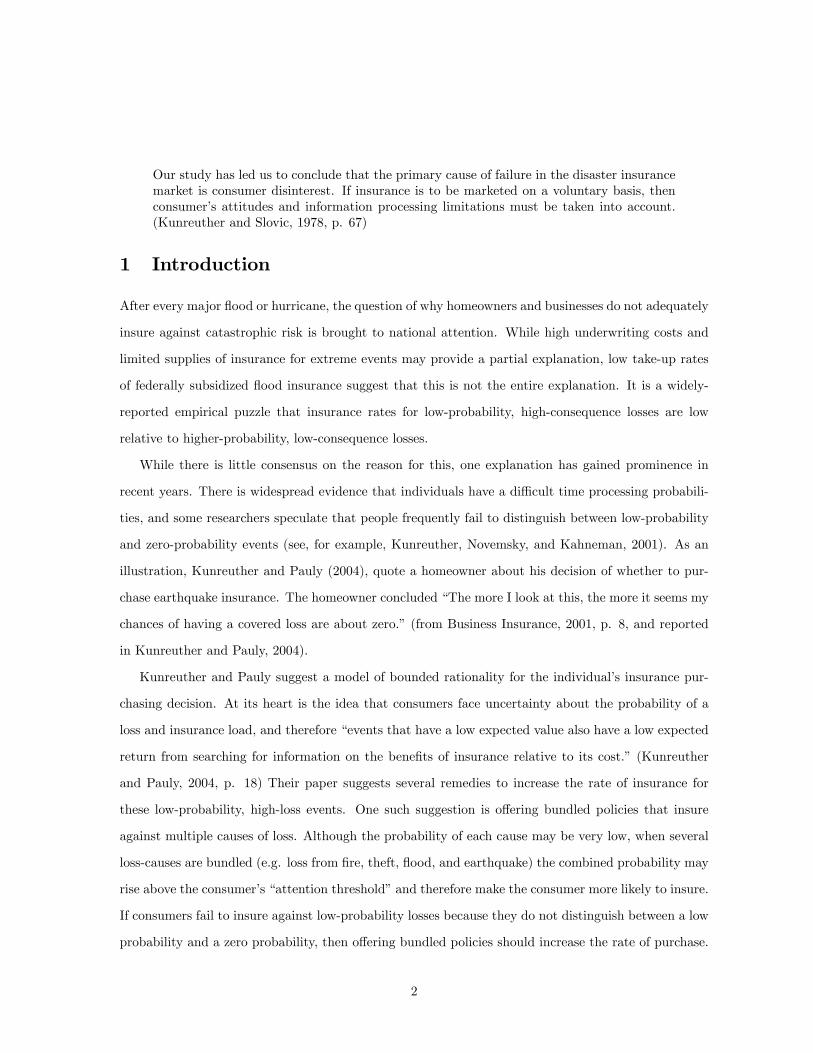
Our study has led us to conclude that the primary cause of failure in the disaster insurancemarket is consumer disinterest. If insurance is to be marketed on a voluntary basis, thenconsumer�s attitudes and information processing limitations must be taken into account.(Kunreuther and Slovic, 1978, p. 67)
1 Introduction
After every major �ood or hurricane, the question of why homeowners and businesses do not adequately
insure against catastrophic risk is brought to national attention. While high underwriting costs and
limited supplies of insurance for extreme events may provide a partial explanation, low take-up rates
of federally subsidized �ood insurance suggest that this is not the entire explanation. It is a widely-
reported empirical puzzle that insurance rates for low-probability, high-consequence losses are low
relative to higher-probability, low-consequence losses.
While there is little consensus on the reason for this, one explanation has gained prominence in
recent years. There is widespread evidence that individuals have a di¢ cult time processing probabili-
ties, and some researchers speculate that people frequently fail to distinguish between low-probability
and zero-probability events (see, for example, Kunreuther, Novemsky, and Kahneman, 2001). As an
illustration, Kunreuther and Pauly (2004), quote a homeowner about his decision of whether to pur-
chase earthquake insurance. The homeowner concluded �The more I look at this, the more it seems my
chances of having a covered loss are about zero.�(from Business Insurance, 2001, p. 8, and reported
in Kunreuther and Pauly, 2004).
Kunreuther and Pauly suggest a model of bounded rationality for the individual�s insurance pur-
chasing decision. At its heart is the idea that consumers face uncertainty about the probability of a
loss and insurance load, and therefore �events that have a low expected value also have a low expected
return from searching for information on the bene�ts of insurance relative to its cost.� (Kunreuther
and Pauly, 2004, p. 18) Their paper suggests several remedies to increase the rate of insurance for
these low-probability, high-loss events. One such suggestion is o¤ering bundled policies that insure
against multiple causes of loss. Although the probability of each cause may be very low, when several
loss-causes are bundled (e.g. loss from �re, theft, �ood, and earthquake) the combined probability may
rise above the consumer�s �attention threshold�and therefore make the consumer more likely to insure.
If consumers fail to insure against low-probability losses because they do not distinguish between a low
probability and a zero probability, then o¤ering bundled policies should increase the rate of purchase.
2
Controlled laboratory experiments are an ideal testbed for policy solutions such as this because one
can control for possibly confounding factors in the lab in a way that is not possible in the �eld. For
example, the probability of an individual loss, insurance load and information can be held constant
between treatments in which individual policies and bundled policies are sold. For this reason, we
conducted a pilot experiment designed to test whether o¤ering bundled policies for several losses
would increase the rate of purchase relative to a treatment in which subjects had to purchase policies
separately for each loss. The results of the pilot presented us with a puzzle: there was no room for
bundling to increase the rate of purchase because subjects in this experiment purchased the individual
policies in almost all cases, even when the probability of an individual loss was quite low.
This result led us to dig more deeply into the experimental literature that reports a positive re-
lationship between the probability of a loss and the rate of insurance purchase (holding constant the
load and expected value of a loss). An extensive review of the literature revealed that the primary
sources for this result were three papers: Slovic, Fischho¤, Lichtenstein, Corrigan and Combs (1977),
McClelland, Schulze, and Coursey (1993), and Ganderton, Brookshire, McKee, Steward, and Thurston
(2000).
The study that most closely resembles naturally-occurring insurance markets is Ganderton et al.
(2000). Subjects earn income each period and, in repeated decision-making rounds, are asked whether
or not they wish to purchase insurance at a stated price. Each subject makes insurance purchase
decisions under a wide range of premiums, loss probabilities and loss amounts. Ganderton et al.
found that the probability of purchasing insurance increases with the probability of a loss, but their
experiment has two features that limit their ability to generalize this result. First, large losses were
nearly always truncated by a low-cost bankruptcy condition such that the ratio of the nominal loss to
the potential for realized losses varied over time and across subjects. Second, the probability and size
of loss were varied independently in their experiments, therefore the expected value of a loss was not
held constant.
McClelland et al. (1993) conducted an earlier experimental study of insurance-purchase decisions.
In this study, real payments were used, but the mechanism used by subjects to purchase insurance
does not closely re�ect the mechanism used in naturally-occurring markets. In this experiment, groups
of eight subjects participated in a Vickrey �fth-price auction, and thus only half of the subjects were
able to buy insurance during a given round. They found a bimodal pattern of bidding; when the
3

probability of a loss was low, bids were most common at zero and twice expected value. Their �nding
that a non-trivial subset of subjects are unwilling to pay any positive amount to insure against a low
probability (p = 0.01) loss persisted even when the stakes were high and subjects were experienced.
These results were interpreted as generally supportive of the artifact that less insurance purchase occurs
at low-probabilities than at higher-probabilities. However, behavioral patterns for bidding in an auction
may not re�ect decision-making patterns in naturally-occurring insurance markets. In fact, Harbaugh,
Kraus, and Vesterlund (2007) o¤er evidence that individuals exhibit sharply di¤erent behavior when
they are o¤ered a choice between gambles over losses and when they are asked to submit a price they
are willing to pay for the same gamble. Naturally-occurring insurance markets more closely resemble
a choice task (consumers choose between a certain loss �the price of insurance �and a probability of a
loss if no insurance is purchased) than a pricing task (submitting a bid to buy insurance in an auction).
Therefore one should be cautions when interpreting results from an auction to make inferences about
purchasing decisions in insurance markets.
The most widely-cited laboratory study of insurance purchasing decisions was conducted by Slovic
et al. (1977). This was a carefully-crafted and well-controlled experiment. Subjects �lled out a
questionnaire that elicited their willingness to purchase actuarially fair insurance in up to eight di¤erent
situations. The probability of a loss was presented in terms of draws of orange and white balls from
an urn, and a loss occurred only when an orange ball was drawn. The probability and size of the loss
were systematically varied across questions, holding constant the expected value of the loss and the
(fair) premium. For example, in one scenario there were 9,999 white balls and 1 orange ball, and the
loss if an orange ball was drawn was 10,000. In another scenario, subjects were told that there were
9,000 white balls and 1,000 orange balls, and the loss if an orange ball was drawn was 10. In each of
the scenarios subjects were asked whether they would purchase insurance at a price of one.
They found that the percentage of subjects purchasing insurance was relatively low (less than
10 percent) when the probability of a loss was very low (and therefore the loss amount was high),
and systematically increased as the probability of a loss increased. While this study was carefully
constructed, two features of the experiment led us to question their results. In almost all of their
treatments, they used hypothetical incentives; subjects were paid for their participation, but not based
upon the answers to the questionnaire. Also, the questions were not framed in terms of monetary
payments and losses. All losses and insurance prices were reported in terms of �points� (e.g., the
4
insurance premium was 1 point in all questions).
Given our concerns about these experiments, we decided to undertake a systematic study of the
e¤ect that the probability of a loss has on insurance purchase decisions. More speci�cally, we study
whether subjects in the lab are more or less likely to purchase insurance against a low-probability loss,
holding constant the expected value of the loss and the insurance load.
We begin by replicating the Slovic et al. study, which we describe in Section 2 below. Next, we
implement a laboratory insurance experiment that more closely resembles naturally-occurring insurance
markets. As we describe in Section 3, subjects earn their initial endowment ($60) and then make a
series of insurance purchase decisions. In some treatments subjects face the loss of their entire earned
endowment.
Our new high-stakes experiment shows that the demand for insurance is high and responds as
expected to increases in load. Moreover, we �nd that the pattern of insurance purchase observed in
earlier experiments is reversed: individuals are more likely to purchase insurance for high-consequence,
low-probability events. Further, we �nd that the results are quite sensitive to whether the stakes
are real. Our results call into question the extent to which the apparent underinsurance observed in
�eld data can be attributed to unwillingness on the part of consumers to purchase catastrophic risk
insurance.
2 Slovic et al. Replication Experiment
First, we report a replication of Slovic et al.�s study. In their experiment, subjects were given a
questionnaire, and asked whether they would purchase insurance in a number of di¤erent hypothetical
situations (six or eight, depending on the treatment). Although complete instructions were not included
in their paper, Slovic et al. did quote extensively from their instructions. To the extent possible, we
used their wording in our instructions (see Appendix A).
Like in Slovic et al., subjects in our experiment were told that they would not play out any of the
gambles that were presented in the questionnaire. The instructions stated:
Each game consists of drawing one ball from each set of baskets. Each contains a di¤erentmixture of orange and white balls. If I were to draw a white ball, no loss would occur. If Iwere to draw an orange ball, this would result a loss, unless you had purchased insurance.(Remember, we will not actually play any of these gambles, but I want you to think abouteach as if you were really going to play each one.)
5

In each situation, the subject was told the number of orange and white balls, the loss if an orange
ball were drawn, and the price of purchasing insurance. The subject was then asked to indicate on the
form whether or not she would purchase insurance in this situation.
We selected parameters to replicate one of the treatments reported by Slovic et al.1 In each
situation, the number of orange and white balls was varied so that the probability of a loss ranged
from .0001 to .50; in every situation, the expected value of a loss was 1 point (so the losses ranged
from 10,000 points to 2 points), and insurance was always actuarially fair (the price of insurance was
held constant at 1 point in each situation). Like Slovic et al. no monetary units were used: all losses
and insurance prices were expressed in points. For example, in one situation, the subject was told the
basket contained 999 white balls and 1 orange ball; if an orange ball was drawn, the individual would
lose 1000 points.
A total of 34 subjects participated in these baseline sessions, which lasted less than one hour.
2.1 Experiment 1 Results
Table 1 presents the percentage of subjects who buy insurance in each of the eight gambles. While
Slovic et al. do not provide a comparable table, we have obtained estimates from a �gure in their
paper and show them for comparison with our results. Subjects in our experiment are more likely to
purchase insurance at low probabilities than those in the Slovic et al. study. Over twenty-�ve percent
of our subjects purchased insurance when the probability of a loss was .0001 or .001, compared with
approximately sixteen percent and twelve percent, respectively, in Slovic et al. However, as shown by
Figure 1, the main feature of their data is replicated in our experiment: the percentage of subjects
purchasing insurance increases as the probability of a loss increases. In our session, twenty-six percent
of subjects say they would buy when the probability of a loss is .0001, compared with forty-seven
percent of subjects who say they would buy when the probability of a loss is 0.01, and sixty-eight
percent when the probability of loss is 0.5.2
Given that we are able to replicate their key �nding, we next turn to an exploration of the robustness
of this phenomenon. We describe a new experiment that tests the pattern of insurance buying behavior
1The level of insurance purchase reported by Slovic et al. varied depending on the treatment, but the overall patternof behavior (higher rates of insurance purchase as the probability of a loss increased) was consistent across treatments.
2The p-value for McNemar�s one-tailed test conditional on the sum of discordant pairs is p=.0096 comparing thepurchase rates for loss probabilities of .001 and .01, and p=.0461 comparing purchase rates for loss probabilities of .01and .5. We provide a more detailed description of McNemar�s test below.
6

#orangeballs
#whiteballs
LossProba-bility
LossAmount
EVLoss
InsurancePrice
SlovicData*
ReplicationData
1 9999 0.0001 10,000 1 1 16% 26%10 9990 0.001 1,000 1 1 12% 29%50 9950 0.005 200 1 1 19% 41%100 9900 0.01 100 1 1 25% 47%500 9500 0.05 20 1 1 48% 59%1000 9000 0.1 10 1 1 64% 62%2500 7500 0.25 4 1 1 69% 71%5000 5000 0.5 2 1 1 62% 68%
*These data are an estimate of their results based on their �gure.
Table 1: Percent Buying Insurance for Slovic et al. Replication
50
60
70
80
nce
Purc
hase
0
10
20
30
40
0.0001 0.001 0.005 0.01 0.05 0.1 0.25 0.5
Pece
nt o
f Ins
uran
Probability of Loss (holding expected value of loss as one)
Slovic et al.
Replication
Figure 1: Comparison of results from Slovic et al. and our replication
7

when the decision problem is framed in terms of monetary losses and monetary costs of insurance, and
when the losses faced by subjects are real and large.
3 New Experiment on the E¤ect of Loss Probability on Insur-
ance Purchase
Moving away from the hypothetical payment and abstract context of the Slovic et al. replication,
we were faced with several challenges in implementing a credible catastrophic loss in the lab. We �rst
describe how we address these design considerations and then describe our treatment variables. After
this we describe the full experimental design, and then present the results from this experiment.
3.1 Implementing Catastrophic Losses in the Lab
There are two features of the naturally-occurring problem that were important to replicate in the lab:
the low probability of a loss, and the high-consequence amount of the loss. For example, the probability
of catastrophic damage from a �ood, �re, or earthquake may be very low; but in the event a loss occurs,
the amount of the loss (including the destruction of one�s home and the loss of belongings) will likely be
very high. In the laboratory, we are challenged to implement losses that are viewed by the participants
as both consequential and �true losses� (and not just lesser gains). The size of the stakes is also of
interest because of recent �ndings showing that individuals appear much more risk averse for high
stakes gambles than low stakes or hypothetical stakes (Camerer and Hogarth, 1999; Holt and Laury,
2002 and 2005; Harrison, Johnson, McInnes and Rutstrom, 2005).
In order to minimize a found-money e¤ect and therefore to make the loss more real to subjects,
they earned their endowments before they faced the insurance-purchase decisions. To ensure that the
potential loss was viewed as substantial, subjects faced the potential loss of all of this earned income
in some situations. In addition, potential losses were never larger than a subject�s available income in
order to avoid confounding the size of losses with bankruptcy considerations.
The only part of a subject�s experiment earnings that was not at risk was a $10 show-up fee. At
the start of the experiment, subjects were paid this show-up fee and signed a receipt for it. Our goal
was for subjects to consider their show-up fee separately from their experiment earnings so that any
8

loss of earned income would be considered a real loss. To this end, subjects were given the following
written statement after signing a receipt for their show-up fee:
In this experiment, you will participate in more than one decision-making task. You willhave the opportunity to earn money in the �rst task. The second task has the possibilityof a negative outcome; if a negative outcome occurs, any money lost will be taken out ofyour earnings from the �rst task.
You have already received $10 for your participation in today�s experiment. This moneyis yours to keep, and you should put it away. You will NOT be asked to risk your $10participation fee in today�s experiment. Any other money that you earn in today�s exper-iment will depend on your choices, and also on chance. However, you will not leave theexperiment with any additional money (other than the $10 participation fee that you havealready received) unless you complete the entire experiment today.
If you wish to withdraw at this time or at any time during the experiment, you may do soand keep your $10 participation fee. Please initial this form to indicate that you understandthis.
All subjects initialed this form and continued their participation in the experiment, and, therefore,
we do not have to be concerned about any sample selection issues.
3.2 Treatments
The primary variable of interest is the probability of experiencing a loss. We chose to use two di¤erent
levels: 1 percent and 10 percent. The choice of probabilities was based on practical considerations and
also guidance from Slovic et al. and our Slovic replication. In both of these prior experiments, there
was a substantial change in the proportion of subjects buying as the probability of a loss increased from
1 percent to 10 percent (from 47 percent to 62 percent buying in our replication, and from about 25
percent to 64 percent reported in Slovic et al.). Therefore, we believed that these two loss-probabilities
would be su¢ cient to test the e¤ect of the probability of a loss on the rate of insurance purchase.
In addition, these probabilities allowed us to determine the outcome of the gamble publicly and in
a manageable way. When the probability of a loss was 1 percent, we placed 1 orange and 99 white
ping-pong balls into a bingo cage. If we had focused on smaller probabilities, this would have required
us to use many more ping-pong balls and therefore we could not have reasonably used a bingo cage to
determine the outcome of the gamble. Instead, these small probabilities would have required us to use
a less transparent manual randomization device or a computerized randomization device. We preferred
the transparency of a manual draw that could be observed by all participants, and so we limited our
attention to this range of probabilities. In addition, in this range of loss probabilities, we could present
9

subjects with the potential loss of the entire endowment without a prohibitively high cash endowment
at the beginning of the experiment. For example, with a loss-probability of .001 and expected value
of a loss of just $0.15, the loss amount would be $150. If the subject were to really face such a loss in
the lab, the initial endowment would have to be at least $150.
Slovic et al. restricted their attention to actuarially fair insurance. However the insurance literature
addresses the issue of under-insurance with respect to subsidized insurance and insurance that is priced
above the expected value of a loss. Based on results from �eld data, the ratio of the premium to expected
bene�t (referred to as the �load� throughout) was set at three levels: 0.80, 1.0, and 4.0. When the
load is set at 0.8, the price of insurance is 80 percent of the expected value of the loss. We included
subsidized insurance because �eld data indicate that individuals fail to purchase insurance against
low-probability events, even when it is heavily subsidized (see Anderson, 1974). When the load is 1.0,
the insurance is actuarially fair, and we are able to compare our results to our replication experiment
in these decisions. When the load is 4.0, the price of insurance is four times the expected value of the
loss. While a load of 4.0 seems high, analyses of non-group health insurance markets (Pauly, Percy
and Herring, 1999) and catastrophic insurance markets (Harrington and Niehaus, 2003) suggests loads
can be as high as 2.5 to 5. By varying the load we can test the robustness of our results to the size
of the load. In addition, by introducing a high load, we may move some of the sample closer to the
margin between buying and not buying insurance and, thus, may have a better chance of observing a
treatment e¤ect as we change the loss probabilities.
In choosing the expected value of the loss, we found little guidance in the literature, but experience
with our subject pool suggests that losses of $30 to $60 are viewed as non-trivial. Because the maximum
possible loss in the experiment could be no larger than the subject�s (earned) endowment (which was
$60 in every case but one), the expected value of the loss was set at three levels: $0.15, $0.30, and
$0.60. While none of these amounts were large compared to the subjects�endowment, the absolute
magnitude of the loss could be signi�cant. For example, a one percent probability of a loss and a $0.60
expected value of a loss imply a one percent chance of losing the entire $60 earned from the initial
earnings task described below.
Combining our choices for load, expected value of loss, and probability of loss, yeilds the 18 decisions
shown in Table 2, and each subject faced all 18 decisions. This represents a within-subjects full-factorial
design of our three main variables: the loss probability (0.01 or 0.10), the expected value of the loss
10

Prob(Loss) EV(Loss) Insurance Load Loss Amount Insurance Premium0.01 0.15 0.8 $15.00 $0.120.01 0.15 1 $15.00 $0.150.01 0.15 4 $15.00 $0.600.01 0.30 0.8 $30.00 $0.240.01 0.30 1 $30.00 $0.300.01 0.30 4 $30.00 $1.200.01 0.60 0.8 $60.00 $0.480.01 0.60 1 $60.00 $0.600.01 0.60 4 $60.00 $2.400.1 0.15 0.8 $1.50 $0.120.1 0.15 1 $1.50 $0.150.1 0.15 4 $1.50 $0.600.1 0.30 0.8 $3.00 $0.240.1 0.30 1 $3.00 $0.300.1 0.30 4 $3.00 $1.200.1 0.60 0.8 $6.00 $0.480.1 0.60 1 $6.00 $0.600.1 0.60 4 $6.00 $2.40
Table 2: Insurance Purchase Decisions from Experiment 2
($0.15, $0.30, $0.60), and the load (0.8, 1.0, 4.0). We describe the exact procedures below.
Finally, we wanted to test whether using real payments mattered, so we conducted some sessions
with hypothetical payments. The hypothetical payment sessions were conducted in an identical manner
to the real-payment sessions with two exceptions: the statement subjects initialed after receiving the
$10 show-up fee did not mention losses, and before the insurance task subjects received the following
written information:
In this part of the experiment, the instructions will describe a series of gambling games.Each game has the possibility of a negative outcome. Each allows you to buy insuranceagainst the negative outcome, although it is not required.
In fact, you will not actually lose any money and I will not take any payment from youin any of these games. Instead, I am going to ask you to consider each of them and tellme how you would play were the earnings described real. Try to take each as seriously aspossible, even though nothing is at stake. We will do everything exactly as described in theinstructions except that we will not take any money from you under any circumstances.
Please initial this sheet of paper to indicate that you understand that all earnings (lossesand payments) are hypothetical for this portion of the experiment and that you will notlose any of the money you earned based on your choices in this part of the experiment.
The �nal treatment (real versus hypothetical) was administered between-subjects; in other words,
a given subject faced all 18 decisions under either real payments or hypothetical payments. Table 3
11

Between SubjectsReal Hypothetical
Probability(0.01, 0.1) $ +
Within Subjects Expected Loss($.15, $.30, $.60) $ +Load(0.8, 1, 4) $ +
Table 3: Summary of Experiment 2 treatments
summarizes the experimental design.
3.3 Experimental Procedures
The experiment consists of a sequence of three phases: the induction, the earnings task, and the
insurance tasks. In the induction, all subjects were seated in the lab, signed a consent form, were paid
a $10 participation payment, and signed a receipt form for this participation payment. As described
earlier, subjects were instructed to put away this money and told they were free to leave with this
payment or continue with the rest of the experiment.
For the earnings task, subjects took a general-knowledge quiz (see Appendix C) and their ex-
periment endowments were determined by their score on the quiz. The subject received $60 if she
answered eight or more questions correctly on the quiz, otherwise she earned $30. This performance-
based payment was used to reinforce the idea that the subject had earned the money (and not just
given the money by the experimenter). However, to avoid confounding the e¤ects of knowledge and
initial endowment, the questions were chosen so that most subjects were expected to earn $60.3 After
quizzes were graded, we came to each subject individually to pay their quiz earnings privately, in cash.
Subjects were encouraged to count the money, but were instructed to leave their earnings on their desk
until the end of the experimental session.
After this initial stake was earned, subjects participated in the insurance task. Instructions were
distributed to all participants (see Appendix E). Subjects were given a chance to read these instructions
on their own, and then they were read aloud. Subjects completed the 18 insurance purchase decisions
shown in Table 2. In each decision (called a �gamble�in the instructions, as in Slovic et al.), subjects
were told the number of orange and white balls that would be used, the loss if an orange ball were
3All but one subject earned $60. The remaining subject was omitted from this analysis.
12

drawn, and the price of insurance. The subject was given a black pen and told to mark on the decision-
sheet whether or not she wished to purchase insurance in this situation. The decisions were given to
subjects one at a time, with the order of presentation varied randomly for each participant. After
completing a decision, subjects were instructed to put their decision sheet into a legal-sized envelope;
when everyone had done so, the next decision sheet was handed out. Thus, after making a decision,
the subject was not able to review or revise any previously-viewed decision.
After everyone had completed all 18 decisions, the black pens were collected and blue pens handed
out.4 Subjects were then told to review all 18 decisions. If a subject wanted to change any of her
decisions, she was told to indicate this on the form with the blue pen. Subjects did not know in advance
that they would be given an opportunity to review any of their decisions. By changing the color of
the pen, we were able to determine whether any subjects changed any decisions at this stage of the
experiment after they had seen all 18 gambles.
After all decisions had been reviewed, they were placed back in the folder and the blue pens were
collected. The experimenter then chose one of these 18 decisions as the binding decision for payment by
drawing a numbered ping-pong ball from a bingo cage. In the instructions, subjects were told that we
would look at only one randomly-determined decision when determining payment and that none of the
other decisions would have any impact on their earnings. All decision sheets were collected, except for
the one chosen for payment. Red pens were then distributed. Subjects were given a �nal opportunity
to review the choice for this one situation before the outcome of the gamble was determined. As before,
subjects were not told in advance that they would have this opportunity to review their choice in the
binding decision. After all subjects had reviewed their choice in the binding decision, the experimenter
came to each person to see if he had purchased insurance. If insurance was purchased, the experimenter
collected the insurance premium out of the subject�s quiz earnings. The appropriate number of orange
and white ping-pong balls were placed in the bingo cage. The color of the ball drawn determined
whether a loss occurred. If an orange ball was drawn, the experimenter came to each person to collect
the loss (unless the subject had purchased insurance). Subjects then completed a short demographic
questionnaire, �lled out a receipt form for experiment earnings, and left the lab.
The experiment, including payment, lasted approximately 90 minutes. A total of 37 subjects
participated in the hypothetical-payment sessions, and 40 subjects participated in the real-payment
4These revision procedures follow Harbaugh et al. (2007).
13

sessions. In the hypothetical-payment sessions, no money was collected from those who purchased
insurance and losses were not collected from uninsured subjects after the realization of a loss event.
4 Results
We �rst present a graphical overview of our data and results from non-parametric statistical tests.
After this, we present results from more formal econometric analysis.
Because each subject completed all 18 decisions, the data for the statistical analysis are �matched
pairs� (each subject serves as her own control). We use McNemar�s exact test statistic for paired
proportions, which takes into account the exact number of discordant pairs (i.e., individuals whose
choices di¤er for the two decisions under comparison). For example, when we test for the e¤ect of a
change in loss probability from 0.01 to 0.10 for fair insurance and an expected value of a loss of $0.15,
we look at the choice (insure or not) for each individual under each of these two treatments and see
whether this individual switched from insuring to not (or from not insuring to insuring).
Treatment averages (the percentage of subjects purchasing insurance) and the corresponding sta-
tistical tests statistics are shown in Table 4, while Figure 2 presents this information in graphical form.
Each panel of the �gure presents the proportion of subjects who chose to purchase insurance when the
probability of a loss was 0.01 (left point) and 0.10 (right point). The left column of this �gure shows
the data for subsidized insurance (load = 0.8), the middle column shows data for fair insurance (load
= 1.0) and the right column shows data for pro�table insurance (load = 4.0). The expected value of
a loss increases from $0.15 in the top row of panels to $0.60 in the bottom row of panels.
The middle column of this Figure corresponds to the Slovic et al. treatment using fair insurance.
For comparison purposes we have included data from our Slovic et al. replication experiment in each of
these three panels as a dashed line. The line joining the Slovic et al. treatment averages has a positive
slope: the proportion of subjects buying insurance was lower for a loss probability of 0.01 than for a
loss probability of 0.10.
It is readily apparent that this behavioral pattern is not replicated in any of our treatments,
except in the hypothetical treatment, when fair insurance is o¤ered against a low ($0.15) expected
value of a loss (for this data pair the proportion buying increases only slightly from 0.49 to 0.54).
In fact, to the extent that the probability of a loss a¤ects insurance purchasing behavior in this new
14

Hypothetical Payment Real PaymentLossProb
LossAmount
EV(Loss)
PercentBuy-ing
McNemar�sTest Sta-tistic
(p-value)
PercentBuy-ing
McNemar�sTest Sta-tistic
(p-value)
Insurance Load = .8 (Subsidized Insurance)0.01 15.00 0.15 62% 0.905 (0.549) 88% 2.668 (0.013)0.1 1.50 0.15 54% 60%
0.01 30.00 0.30 65% 1 (0.455) 0.90% 2.324 (0.035)0.1 3.00 0.30 54% 0.68%
0.01 60.00 0.60 68% 0 (1) 90% 0 (1)0.1 6.00 0.60 68% 90%
Insurance Load = 1 (Fair Insurance)0.01 15.00 0.15 49% -0.58 (0.774) 85% 2.84 (0.007)0.1 1.50 0.15 54% 58%
0.01 30.00 0.30 51% 0.302 (1) 90% 2.324 (0.035)0.1 3.00 0.30 49% 68%
0.01 60.00 0.60 59% 0 (1) 90% 0 (1)0.1 6.00 0.60 59% 90%
Insurance Load = 40.01 15.00 0.15 46% 1.732 (0.146) 85% 4.583 (0.000)0.1 1.50 0.15 30% 33%
0.01 30.00 0.30 41% 2.646 (0.016) 83% 3.771 (0.000)0.1 3.00 0.30 22% 43%
0.01 60.00 0.60 49% 2.111 (0.065) 85% 3.153 (0.0030.1 6.00 0.60 30% 53%
Table 4: Insurance Purchase Percentages for Experiment 2
experiment, the proportion purchasing is lower when the probability of a loss is 0.10 compared to 0.01.
As indicated by the asterisks in the Figure, this di¤erence is signi�cant for most comparisons in the
real-payment treatment. The only exceptions are for the largest losses: when the expected value of
a loss is $0.60 and the insurance is subsidized or fair, 90 percent of all subjects in the real-payment
sessions purchase insurance regardless of the loss probability. However, when the insurance carries a
high load, signi�cantly more subjects insure when the loss probability is 0.01 than when it is 0.10.
In the hypothetical payment sessions, fewer subjects purchase insurance than in the corresponding
real payment sessions. And while the pattern of purchase decisions is similar to that in the real-
payment sessions, the di¤erence in the proportion of subjects buying insurance as the loss probability
15

0.8
1
0.8
1
0.8
1
* *
0
0.2
0.4
0.6
01 10
0.2
0.4
0.6
01 10
0.2
0.4
0.6
01 1
EVloss .15Load .8
EVloss .15Load 1
EVloss .15Load 4
*
p=.01 p=.1 p=.01 p=.1 p=.01 p=.1
0.4
0.6
0.8
1
0.4
0.6
0.8
1
0.4
0.6
0.8
1
real
hypothetical
Slovic*
***
0
0.2
p=.01 p=.10
0.2
p=.01 p=.10
0.2
p=.01 p=.1
Slovic replication
0 8
1
0 8
1
0 8
1
EVloss .30Load .8
EVloss .30Load 1
EVloss .30Load 4
0
0.2
0.4
0.6
0.8
0
0.2
0.4
0.6
0.8
0
0.2
0.4
0.6
0.8
EVloss .60Load .8
EVloss .60Load 1
EVloss .60Load 4
*
0p=.01 p=.1
0p=.01 p=.1 p=.01 p=.1
* Significant difference at the 5 percent level using a two-sided McNemar’s test
Figure 2: Proportion of insurance purchases for loss probabilities 0.01 and 0.1, conditioned on expectedloss and load
changes is generally not signi�cantly di¤erent than zero.
We also estimate a panel logistic regression model of insurance purchase and the results are con-
sistent with the nonparametric analysis presented above. The regression assumes a threshold crossing
model in which individuals purchase insurance when the net bene�t is positive. For a risk-averse
expected-utility maximizer, the net bene�t of insurance increases in the probability of loss (holding
the expected loss constant). Random e¤ects are included to allow for unobserved individual di¤erences
that may a¤ect the propensity to insure but are assumed to be uncorrelated with treatment parame-
ters due to the randomized design. We estimate separate models for hypothetical- and real-payment
16

Hypothetical Payment Real Payment PooledProb(Loss) -25.603 -6.159 -25.939
(3.006)** (2.318)** (2.986)**Load -0.495 -0.492 -0.503
(0.081)** (0.075)** (0.081)**EV(Loss) 3.230 1.145 3.275
(0.666)** (0.557)* (0.667)**Hypothetical -2.514
(0.719)**Interaction: Hyp x Prob(Loss) 19.846
(3.758)**Inteaction: Hyp x Load 0.016
(0.109)Interaction: Hyp x EV(Loss) -2.142
(0.865)*Constant 3.377 0.953 3.453
(0.522)** (0.512) (0.533)**Observations 720 666 1386Number of Subjects 40 37 77
Standard errors in parentheses. Statistical signi�cance at 5% (1%) denoted with * (**).
Table 5: Random E¤ects Logistic Models of the Probability of Purchasing Insurance
sessions, as well as a pooled speci�cation with an indicator variable for the type of incentives and a
full set of interactions for hypothetical incentives. We also report regressions that include individual
demographic and insurance purchase data gathered from the post-experiment questionnaire.
The regression results in Table 5 show that the probability of purchasing insurance is positively and
signi�cantly related to the probability of loss holding expected loss and load constant. Hypothetical
incentives signi�cantly reduce the likelihood of purchasing insurance and mitigate the sensitivity to
the probability of loss. The regression results in Table 5 also show that load and the magnitude
of the expected loss a¤ect purchase rates. Under both real and hypothetical incentives, participants
responded rationally to increases in the load by decreasing purchase rates. We also see that participants
were more likely to insure against larger expected losses than smaller ones, but the e¤ect was greater
when the incentives were real.
After completing the experiment, participants were asked to �ll out a short questionnaire asking
about their demographic characteristics and whether or not they had purchased common forms of
insurance and extended warranties. The descriptive statistics for their responses are shown in Appendix
D. Adding this demographic and insurance purchase experience to the regressions made little di¤erence
to the main results. Age was the only variable found to have a signi�cant e¤ect on purchase rates.
17

Larger samples may be needed in order to identify the relationships between the decision to insure in
the lab and demographic characteristics or other (naturally occurring) insurance purchases.
As a robustness check, we re-analyzed the data using each individual�s initial decision about whether
or not to purchase insurance. In the experiment, individuals made 18 decisions in random order and
then were given the opportunity to review all decisions and make any desired changes. About half of
all subjects changed at least one of their decisions of whether to buy insurance. In the real-payment
sessions, most switches (75%) were from not buying insurance to buying insurance while the switches
in the hypothetical-payment sessions were about evenly split. Because changes in the purchase decision
may represent corrections of recording errors or learning over the course of the experiment, the revised
decisions may be less noisy. Using initial decisions rather than revised decisions makes no di¤erence in
the analysis.
5 Conclusions
It has been widely accepted that individuals tend to under-insure against low-probability, high-loss
events relative to high-probability, low-loss events. When people fail to insure against catastrophic
losses, the social and economic costs of this can be quite large. If our goal is to develop a policy solution
to this problem, it is important to understand why so many people fail to purchase this insurance. For
example, if consumers do not process low probabilities accurately, then o¤ering bundled policies may
remedy the problem. On the other hand, if they do not insure because the insurance is too expensive
(or carries too high of a load), then o¤ering credible, subsidized insurance should help.
In this experiment, we implemented real, high-consequence losses in the lab. Our focus was on how
individuals respond to changes in the probability of a loss. The conventional wisdom is that people
misperceive probabilities and fail to distinguish between low-probability events and those with zero
probability. This conventional wisdom and prior experimental evidence predicted that subjects would
purchase less insurance with a loss-probability of 1 percent than with a loss probability of 10 percent.
In contrast, our experiment suggests that people are no less likely to insure against low-probability,
high-loss events when compared to higher-probability losses of equal expected value. Therefore a policy
that focuses on probability misperceptions is fundamentally misguided and may not solve the problem
of under-insurance in the �eld. Instead, policies that focus on other explanations for under-insurance
18

(moral hazards and high loads, for example) may be more successful. Future experiments will explore
the underlying causes of this behavioral regularity.
19
References
[1] Anderson, D. R. (1974) �The National Flood Insurance Program: Problems and Potential�Journal
of Risk and Insurance, 41, 579-599.
[2] Camerer, C. and R. Hogarth, 1999, �The e¤ects of �nancial incentives in experiments: a review
and capital- labor-production framework,�Journal of Risk and Uncertainty 19, 7-42.
[3] Cutler and Zeckhauser. (2004) �Extending the Theory to Meet the Practice of Insurance�
Brookings-Wharton Papers on Financial Services, 2004, 1-53.
[4] Ganderton, Philip T., David S. Brookshire, Michael McKee, Steve Steward, and Hale Thurston.
(2000) �Buying Insurance for Disaster-Type Risks: Experimental Evidence�Journal of Risk and
Uncertainty 20(3), 271-89.
[5] Harbaugh, Kraus, and Vesterlund (2007) �The Fourfold Pattern of Risk Attitudes in Choice and
Pricing Tasks�University of Oregon Working Paper.
[6] Harrington, Scott, and Gregory Niehaus. (2003) �Capital, Corporate Income Taxes, and Catastro-
phe Insurance, Journal of Financial Intermediation 12, 365-389.
[7] Harrison, Glenn, Eric Johnson, Melayne McInnes, and Elisabet Rutstrom. (2005). "Risk Aversion
and Incentive E¤ects: Comment," American Economic Review 95(3), 897-901.
[8] Holt, Charles and Susan Laury. 2002. �Risk Aversion and Incentive E¤ects.�American Economic
Review 92(5), 1644-1655.
[9] Holt, Charles and Susan Laury. 2005. �Risk Aversion and Incentive E¤ects: New Data without
Order E¤ects,�American EconomicReview 95(3), 2005, 902-912.
[10] Kunreuther, Howard. (1984). �Causes of Underinsurance against Natural Disasters,�The Geneva
Papers on Risk and Insurance 31, 206-20.
[11] Kunreuther, Howard, R. Ginsberg, L. Miller, P. Sagi, P. Slovic, B. Borkan, and N. Katz, (1978),
Disaster Insurance Protection: Public Policy Lessons, New York: Wiley.
[12] Kunreuther, Howard, Nathan Novemsky, and Daniel Kahneman. (2001). �Making Low Probabil-
ities Useful,�Journal of Risk and Uncertainty 23, 103-120.
20

[13] Kunreuther, Howard and Mark Pauly. (2004). "Neglecting Disaster: Why Don�t People Insure
Against Large Losses?," Journal of Risk and Uncertainty, 28(1), 5-21.
[14] Kunreuther, Howard and Paul Slovic. (1978). "Economics, Psychology, and Protective Behavior,"
The American Economic Review, Vol. 68, No. 2, Papers and Proceedings of the Ninetieth Annual
Meeting of the American Economic Association. 64-69.
[15] McClelland, G.H., Schulze, W. D., & Coursey, D. L. (1993). �Insurance for low-probability hazards:
a bimodal response to unlikely events.�Journal of Risk and Uncertainty, 7(1), 95-116.
[16] Pauly, Mark, Allison Percy and Bradley Herring. (1999). "Individual vs. Job-Based Health Insur-
ance: Weighing the Pros and Cons," Health A¤airs, Vol. 18(6), 28-44.
[17] Slovic, Fischho¤, Lichtenstein, Corrigan and Combs (1977) �Preference for Insuring against Prob-
able Small Losses: Insurance Implications�Journal of Risk and Insurance, 237-257
A Instructions for Slovic et al. Replication
In this survey, I am going to describe a series of gambling games. Each game has the possibility ofnegative outcomes. Each allows you to buy insurance against the negative outcomes, although it isnot required. I am not going to ask you to play any of the games. Instead, I am going to ask you toconsider each and then tell me how you would play were they for real. Try to take each as seriously aspossible, even though nothing is at stake.Each game consists of drawing one ball from each set of baskets. Each contains a di¤erent mixture
of orange and white balls. If I were to draw a white ball, no loss would occur. If I were to draw anorange ball, this would result a loss, unless you had purchased insurance. (Remember, we will notactually play any of these gambles, but I want you to think about each as if you were really going toplay each one.)As you can see, you can only lose in this sort of game (either by drawing an orange ball or by
buying insurance). Your object is to lose as little as possible. For each game �gure out what insuranceyou would buy to end up with the fewest negative points.
B General Knowledge Quiz
The following questions test your knowledge of current events, American history, and geography. Pleaseindicate the correct answer in the blank beside each question. You will be paid based on the numberof questions you answer correctly.
If you answer 8 or more questions correctly, you will be paid $60.If you answer 7 or fewer questions correctly, you will be paid $30
______1. The current Secretary of State isa. Dick Cheneyb. John Snow
21
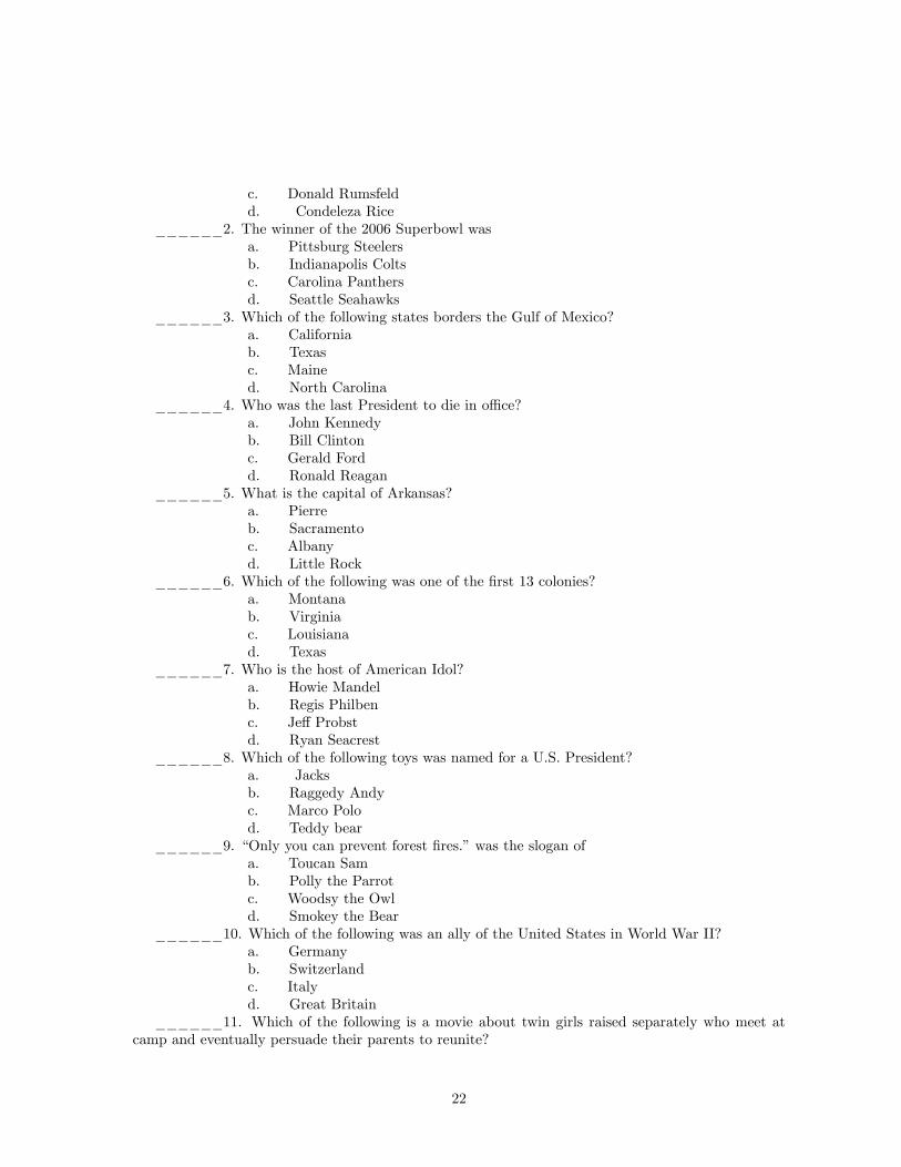
c. Donald Rumsfeldd. Condeleza Rice
______2. The winner of the 2006 Superbowl wasa. Pittsburg Steelersb. Indianapolis Coltsc. Carolina Panthersd. Seattle Seahawks
______3. Which of the following states borders the Gulf of Mexico?a. Californiab. Texasc. Mained. North Carolina
______4. Who was the last President to die in o¢ ce?a. John Kennedyb. Bill Clintonc. Gerald Fordd. Ronald Reagan
______5. What is the capital of Arkansas?a. Pierreb. Sacramentoc. Albanyd. Little Rock
______6. Which of the following was one of the �rst 13 colonies?a. Montanab. Virginiac. Louisianad. Texas
______7. Who is the host of American Idol?a. Howie Mandelb. Regis Philbenc. Je¤ Probstd. Ryan Seacrest
______8. Which of the following toys was named for a U.S. President?a. Jacksb. Raggedy Andyc. Marco Polod. Teddy bear
______9. �Only you can prevent forest �res.�was the slogan ofa. Toucan Samb. Polly the Parrotc. Woodsy the Owld. Smokey the Bear
______10. Which of the following was an ally of the United States in World War II?a. Germanyb. Switzerlandc. Italyd. Great Britain
______11. Which of the following is a movie about twin girls raised separately who meet atcamp and eventually persuade their parents to reunite?
22

a. Freaky Fridayb. The Pajama Gamec. The Parent Trapd. Yours, Mine and Ours
______12. Which television network carries the OC?a. Foxb. PBSc. HBOd. MTV
______13. �Scrubs�is a television series centered arounda. a carwashb. a hospitalc. a baseball teamd. hotel maid service
______14. Who is credited with inventing the light bulb?a. Eli Whitneyb. Oprah Winfreyc. Thomas Edisond. Enrico Marconi
______15. �First in Flight�is the slogan of which of the following states?a. Texasb. Montanac. Mained. North Carolina
C Experiment Instructions
Today you will make choices about a series of gambles. Each gamble has the possibility of a negativeoutcome. In each gamble, you will be allowed to buy insurance against the negative outcome, althoughyou are not required to buy the insurance.Each gamble consists of drawing one ball from a basket. Each basket contains a di¤erent mixture
of orange and white balls. If I draw a white ball, no loss occurs. If I draw an orange ball, this willresult in a loss. Any loss you incur will be paid out of the money you earned by taking the CurrentEvents Quiz, unless you choose to purchase insurance.Here is how this will work: if you choose to purchase insurance, you will pay for this out of the
money that you earned by taking the Current Events Quiz. If you do not purchase insurance and Idraw a white ball, you will keep all of the money that you earned. If you do not purchase insuranceand I draw an orange ball, you will lose some or all of the money that you earned by taking the CurrentEvents Quiz. Each gamble will specify how much you may lose and how much the insurance will cost.Each gamble that you face will be similar to the following (though the numbers used in the exper-
iment will be di¤erent than this example):
23

.
Gamble 0
Orange Balls White Balls
Number in Basket 5 95
Loss if Drawn $12.00 $0
Insurance Premium: $12.00
Yes No
Do you want to purchase insurance for $1.20?
Indicate your answer by placing an X in the appropriate box above.
If this is the gamble that is chosen: 1. Only your insurance decision on this
sheet will be considered; and 2. If you purchase insurance for this
gamble, you will pay for it before we draw a ball from this basket.
If you faced the gamble in this example and you chose to purchase insurance you would pay me$1.20 from the money you earned by taking the Current Events Quiz. You would pay this $1.20 beforeI drew a ball from the basket, so you would pay it regardless of whether I drew a white ball or anorange ball. However, if you purchased this insurance and I drew an orange ball, you would not lose$12 in this example.You will make decisions for 18 gambles during this part of the experiment. You should read the
information provided to you in each one carefully: the number of orange and white balls, the loss youincur if an orange ball is drawn, and the insurance premium may change from one gamble to another.Even though you will face 18 gambles in this experiment, only ONE of them will be used to
determine your earnings. After you have made all 18 choices, we will put 18 numbered ping-pongballs into a cage. We will mix up these balls and then draw one ball from the cage. The number thatappears on the ball that we draw will determine which choice will count.For example, if we drew a ball with a 12 written on it, only your choice in Gamble 12 would count.
None of your other choices would have any e¤ect on your earnings. If you chose to purchase insurancein Gamble 12, you would pay the stated price of insurance in this decision. If you did not choose topurchase insurance in Gamble 12, the color of the ball drawn in this gamble would determine whetheryou lost any money in this experiment.Even though only one of your 18 choices will count, you will not know in advance which gamble will
be used to determine your earnings. Therefore, you should think about each of them carefully beforesubmitting your choice.Although each of you will make 18 choices, you may not face the same 18 gambles. Also, we have
already shu ed your decision-sheets so each of you will receive your gambles in a di¤erent order. Forexample, one person may see Gamble 5 and then Gamble 3, while another person may see Gamble 7�rst, and then Gamble 10. However, each of you will make decisions in 18 di¤erent gambles.To summarize, this is what will happen during the rest of today�s experiment:1. We will show you 18 gambles; in each you must choose whether or not you wish to purchase
insurance at the stated price. We will show you these gambles one at a time. After everyone has madetheir �rst choice, we will show you a second gamble, and so on for all 18 gambles.2. After everyone has made all 18 choices, we will draw a numbered ping-pong ball to determine
which ONE of these gambles will count. We will not look at your choices for any other gamble whendetermining your earnings.3. We will come to each of you and see if you chose to purchase insurance in this gamble. If you
purchased insurance, we will collect the stated price of insurance from you.4. We will place into this bucket the number of orange and white ping-pong balls speci�ed in the
24

gamble.5. We will mix up these ping-pong balls and then draw ONE ball from the bucket.6. If we draw a white ball, no one will incur a loss. If we draw an orange ball, you will lose the
amount speci�ed in this gamble, unless you chose to purchase insurance.7. You will sign a receipt form and then may leave the experiment.We ask that you not talk to one another during this experiment. If you have any questions at any
time, please raise your hand and one of us will come to you to answer the question. Before we begindo you have any questions about these procedures or how your earnings will be determined?
D Descriptive Statistics for Demographic and Insurance Pur-chase Questionnaire
Table D1: Demographics and Insurance Purchase Experience
Variable Obs. Mean Std.Dev. Min. Max.Score on Quiz 77 12.31 2.00 4 15Age 77 21.42 2.98 18 36Gender is male 77 0.52 0.50 0 1White 77 0.16 0.37 0 1Black 77 0.61 0.49 0 1Asian 77 0.14 0.35 0 1Raised in U.S. 76 0.88 0.33 0 1Bought Renters Insurance 77 0.10 0.31 0 1Bought Homeowners Insurance 77 0.01 0.11 0 1Bought Car Insurance 77 0.51 0.50 0 1Bought Health Insurance 77 0.34 0.48 0 1Bought Extended Warranty 77 0.34 0.48 0 1
25

Table D2: Logistic Regression Models of Probability of Purchasing Insurance with Demographics
Pooled Payment Pooled PaymentProb(Loss) -31.400 -26.077
(3.381)** (2.999)**Load -0.575 -0.505
(0.088)** (0.082)**EV(Loss) 3.684 3.293
(0.718)** (0.669)**Hypothetical -2.914 -2.659
(0.748)** (0.714)**Interaction: Hyp x Prob(Loss) 25.253 20.007
(4.081)** (3.765)**Interaction: Hyp x Load 0.084 0.020
(0.115) (0.109)Interaction: Hyp x EV(Loss) -2.541 -2.164
(0.906)** (0.866)*Score of Current Event Quiz 0.063
(0.158)Age 0.251
(0.114)*Gender -0.612
(0.595)Caucasian -0.647
(0.812)Asian -0.967
(0.893)US Raised -0.493
(0.992)Purchased Car Insurance -0.670
(0.563)Purchased Extend Warranty -0.212
(0.604)Purchased Health Insurance 0.972
(0.629)Purchased Renters or Homeowners 0.932
(0.912)Constant -1.288 3.517
(3.274) (0.638)**Observations 1368 1386Number of Subjects 76 77
* is statically signi�cant at 5%; ** is statistically sign�cant at 1%
26