Embed Size (px)
Citation preview
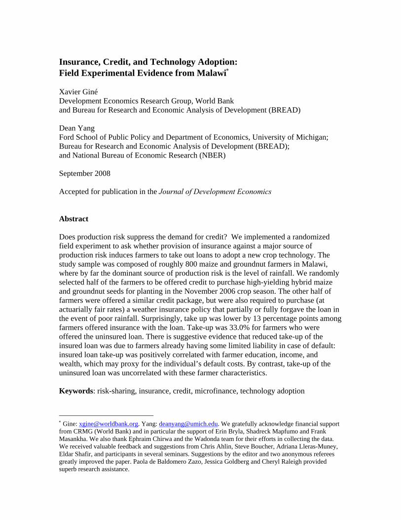
Insurance, Credit, and Technology Adoption: Field Experimental Evidence from Malawi∗ Xavier Giné Development Economics Research Group, World Bank and Bureau for Research and Economic Analysis of Development (BREAD) Dean Yang Ford School of Public Policy and Department of Economics, University of Michigan; Bureau for Research and Economic Analysis of Development (BREAD); and National Bureau of Economic Research (NBER) September 2008 Accepted for publication in the Journal of Development Economics Abstract Does production risk suppress the demand for credit? We implemented a randomized field experiment to ask whether provision of insurance against a major source of production risk induces farmers to take out loans to adopt a new crop technology. The study sample was composed of roughly 800 maize and groundnut farmers in Malawi, where by far the dominant source of production risk is the level of rainfall. We randomly selected half of the farmers to be offered credit to purchase high-yielding hybrid maize and groundnut seeds for planting in the November 2006 crop season. The other half of farmers were offered a similar credit package, but were also required to purchase (at actuarially fair rates) a weather insurance policy that partially or fully forgave the loan in the event of poor rainfall. Surprisingly, take up was lower by 13 percentage points among farmers offered insurance with the loan. Take-up was 33.0% for farmers who were offered the uninsured loan. There is suggestive evidence that reduced take-up of the insured loan was due to farmers already having some limited liability in case of default: insured loan take-up was positively correlated with farmer education, income, and wealth, which may proxy for the individual’s default costs. By contrast, take-up of the uninsured loan was uncorrelated with these farmer characteristics. Keywords: risk-sharing, insurance, credit, microfinance, technology adoption
∗ Gine: [email protected]. Yang: [email protected]. We gratefully acknowledge financial support from CRMG (World Bank) and in particular the support of Erin Bryla, Shadreck Mapfumo and Frank Masankha. We also thank Ephraim Chirwa and the Wadonda team for their efforts in collecting the data. We received valuable feedback and suggestions from Chris Ahlin, Steve Boucher, Adriana Lleras-Muney, Eldar Shafir, and participants in several seminars. Suggestions by the editor and two anonymous referees greatly improved the paper. Paola de Baldomero Zazo, Jessica Goldberg and Cheryl Raleigh provided superb research assistance.

1
1. Introduction
A great deal of attention is paid to imperfections in credit markets as barriers to
growth in rural areas of developing countries. Most prominently, the literature has
emphasized limitations in the supply of credit due to asymmetric information and
imperfect enforcement. The problems that arise can often be characterized by a
borrower’s inability to commit to fulfilling a debt contract. Debtors cannot credibly
reveal their borrowing type truthfully (adverse selection), promise to exert effort so that
their production enterprise does not fail (ex-ante moral hazard), report their production
output honestly (ex-post moral hazard), or promise to repay the loan even when output
was sufficient (opportunistic default).1
A second type of credit market imperfection is due to the absence of or limitations
in insurance markets. Uninsured borrowers may be deterred from taking on loans by the
risk of high default costs (e.g., confiscation of assets) in states of the world where income
is low and they are unable to repay the loan. Binswanger and Sillers (1983) and Boucher,
Carter, and Guirkinger (2008) have emphasized so-called “risk rationing,” or risk-
motivated voluntary withdrawal from the credit market.2
This paper focuses on the second of these two categories of credit market
imperfections. We conducted a randomized field experiment to determine whether
bundling insurance with a loan (intended to finance adoption of a new crop technology)
increased demand for the loan. The specific context of the study was the adoption of
high-yield hybrid varieties of maize and groundnut among smallholder farmers in
Malawi.
To test the importance of risk in hindering take-up of loans for hybrid seed
adoption, we randomized whether farmers’ loans were insured against rainfall risk, by far
the dominant source of production risk in Malawi. The study sample was composed of
roughly 800 maize and groundnut farmers in 32 localities in central Malawi. We
randomly selected 16 localities where farmers were offered credit to purchase high-
1 For comprehensive reviews of this literature, see Dowd (1992), Ghosh, Mookherjee and Ray (2000), and Conning and Udry (2005). 2 Relatedly, Dercon and Christiaensen (2007) argue that consumption risk discourages fertilizer use by Ethiopian farmers.

2
yielding hybrid maize and groundnut seeds for planting in the November 2006 crop
season. In the remaining 16 localities, farmers were offered a similar credit package, but
were also required to purchase (at actuarially fair rates) a weather insurance policy that
partially or fully forgave the loan in the event of poor rainfall.
If borrowers are risk averse while the lender is not, a standard debt contract
(credit only) will in general not be optimal because it requires that the borrower bear all
the risk when he or she is the least prepared to bear it. But in the presence of
informational asymmetries (requiring verification costs) or under bounded rationality, the
simplicity of the debt contract may indeed be close to being optimal (Dowd 1992).
In any event, the requirement in a debt contract that repayment be non-contingent
may be responsible for a lower demand for credit as prospective borrowers fear the loss
in utility associated to having to repay even when production fails. In other words, risk
averse borrowers may prefer planting a traditional variety that does not require credit, to
adopting the hybrid variety that is riskier. In this situation, the provision of insurance
should in principle raise adoption among risk-averse farmers.
Our experimental results are at odds with this prediction. Take-up was 33.0%
among farmers who were offered the basic loan without insurance. Take up was lower, at
only 17.6%, among farmers whose loans were insured against poor rainfall. A potential
explanation is that farmers already are implicitly insured by the limited liability inherent
in the loan contract, so that bundling a loan with formal insurance (for which an
insurance premium is charged) is effectively an increase in the interest rate on the loan.
We offer suggestive evidence in support of this hypothesis: among farmers offered the
insured loan, take-up is positively associated with a farmer’s education, income, and
wealth. These variables may proxy for the farmer’s income in the low state (a measure of
default costs, if crop output can be seized by the lender), and if so should be correlated
with the benefit a farmer can expect from insurance. By contrast, for farmers offered the
uninsured loan, these characteristics are not associated with take-up.
In addition to shedding light on the interactions between credit and insurance
markets, this paper also contributes to our understanding of technology adoption in rural
areas of developing countries. The adoption of new technology plays a fundamental role
in the development process. In the 1950s and 1960s, the so-called Green Revolution

3
transformed agricultural production in developing countries by introducing high-yield
crop varieties and other modern cultivation practices. While the modernization of
production brought about significant increases in agricultural productivity and growth,
the impact of the Green Revolution has been uneven. There is enormous variation, within
regions and between regions, in the extent to which households have benefited from the
availability of these new technologies.8 Nearly all Malawian households (97% in 2004-
2005) are engaged in maize production, but only 58% use hybrid maize varieties (World
Bank 2006). Smale and Jayne (2003) note that hybrid maize adoption in Malawi has
lagged behind adoption in Kenya, Zambia, and Zimbabwe.
Among the often cited reasons why technology has failed to diffuse, aversion to
risk, credit constraints and limited access to information are leading candidates (Feder,
Just and Zilberman, 1985).9 Undoubtedly, production risk is a major source of income
fluctuations for rural households involved in agricultural activities, especially in
developing countries. Because high yield varieties are more profitable but also riskier,
households unwilling to bear consumption fluctuations may decide not to adopt. In
addition, in policy circles the lack of access to credit has traditionally been considered a
major obstacle to technology adoption and development.10
With complete and frictionless financial markets, fluctuations would not be a
source of concern as households would be able to protect consumption, and credit would
flow to activities with the highest marginal return. But in developing countries, insurance
and credit markets are typically incomplete or altogether absent. In this environment, the
separation of consumption and production decisions may not obtain (Benjamin, 1992),
and thus, the relative importance of credit constraints and risk aversion may be
confounded (Chaudhuri and Osborne, 2002).
8 See Griliches (1957) on adoption of hybrid corn in the United States, Evenson (1974) on diffusion of agricultural technologies internationally, and Goldman (1993) on technology adoption across regions in Kenya. 9 See Evenson and Westphal (1995), Rogers (1995) and Munshi (forthcoming) for a more recent review. See also the introduction in Conley and Udry (2005) for references, as well as Besley and Case (1994). Recent work on technology adoption and social learning includes Foster and Rosenzweig (1995), Munshi (2004), Conley and Udry (2005), and Duflo, Kremer, and Robinson (2006). 10 The following quote from 1973 by Robert McNamara when he was the World Bank president exemplifies this view: “The miracle of the Green Revolution may have arrived, but for the most part, the poor farmer has not been able to participate in it. He simply cannot afford to pay for the irrigation, the pesticide, the fertilizer… For the small holder operating with virtually no capital, access to capital is crucial”.
4
This last point is illustrated by the well-known positive correlation between
wealth and adoption of new technology.11 Existing studies document that hybrid seed use
in Malawi is correlated with wealth and other indicators of household socioeconomic
status. Data from the country’s nationally-representative Integrated Household Survey
conducted in 2004-2005 documents higher adoption of hybrid maize among households
in the highest quintile of land ownership (66%) than in the lowest quintile (53%) (World
Bank 2006). Among maize farmers in southern Malawi, Chirwa (2005) finds that close to
60% do not use hybrid maize varieties, and that adoption rises in income, education, and
plot size. Simtowe and Zeller (2006) find higher maize adoption among households with
access to credit. Due to the potential correlation between access to credit and ability (or
willingness) to cope with risk, it is unclear in these studies whether credit constraints or
absence of insurance markets (or both) are the key constraints hindering hybrid seed
adoption in Malawi (and elsewhere). Disentangling the two explanations is crucial
because they call for very different government interventions.
Our findings are also related to existing research documenting relatively limited
demand for weather insurance in developing countries. Our theoretical model where
borrowers’ limited liability limits the value of formal weather insurance is reminiscent of
Rosenzweig and Wolpin (1993), who show in simulations that the gain from weather
insurance for Indian farmers is minimal due the existence of informal insurance
mechanisms that create a consumption floor. Giné, Townsend, and Vickery (2008) find
relatively low take-up (4.6%) of a standalone rainfall insurance policy among farmers in
rural Andhra Pradesh, India in 2004. Using door-to-door marketing visits, Cole et al.
(2008) find substantially higher take-up (27%) in 2006 among the same sample of
farmers in Andhra Pradesh and a take-up of 23% of another standalone rainfall insurance
policy in rural Gujarat, India. They also find that variations in marketing can have
substantial impact on the take-up. Both Giné, Townsend, and Vickery (2008) and Cole et
al. (2008) find, as we do in this paper, that take-up is correlated with farmers’ wealth.
Their story is one of credit constraints: since the insurance policy must be purchased at
the onset of the season, coinciding with the purchase of the other agricultural inputs
(labor for land preparation, seeds, fertilizer, etc.) there are competing uses for the cash
11 See Feder, Just, and Zilberman (1985), Just and Zilberman (1983), Besley and Case (1993).
5
and only the better-off can afford the policy. In the Malawi field experiment we examine
in the current paper, there is also a deposit that needs to be paid upfront, but the fact that
wealth and income matter for the insured loan but not for the uninsured loan suggest that
something other than credit constraints may be at play.
The remainder of this paper is organized as follows. In Section 2 we present a
simple model that is consistent with the lower take-up in the insured group. In Section 3
we describe the experimental design and the survey data. We describe the main empirical
results on the impact of the insurance on take-up in Section 4, and then in Section 5
explore the determinants of take-up separately in the treatment and control groups.
Section 6 discusses additional explanations for lower take-up in the insured group.
Section 7 concludes. The Appendix provides further details on the variables used in the
empirical analysis.
2. A Simple Model
Why were farmers less likely to take up the loan for the hybrid or improved seeds
when it was bundled with insurance? To fix ideas, we present a simple model of a risk-
averse household that is deciding whether or not to take up the package. The benchmark
model predicts that the value that farmers attach to the explicit insurance bundled with the
loan is negatively related to the implicit insurance in the loan contract provided by the
limited liability constraint. Indeed, when the maximum that lenders can seize is the value
of production, the loan contract provides insurance to borrowers because repayment is
already contingent: in case of production failure, borrowers repay less. Under certain
conditions, risk-averse agents could prefer not to adopt the hybrid seeds if the loan was
bundled with insurance at an actuarially fair price, but they would adopt them if a
standard (uninsured) loan contract was offered. If, on the other hand, farmers could
always repay the bank, the loan would no longer provide implicit insurance because the
limited liability constraint would never bind. In this case, a risk-averse farmer should be
unambiguously better off when the loan is bundled with insurance.
To formalize the argument, imagine a farmer that can grow a crop using either
traditional or hybrid seeds. Output from traditional seeds is TY . Hybrid seeds have higher
6
average yields but are riskier: YH with probability p and YL with probability 1-p and
(1 )T H LY pY p Y< + − . In addition, the seeds are costly, so assuming no liquid wealth, the
farmer needs to borrow from a bank to be able to purchase them. Assume that the bank
offers a standard debt contract (uninsured loan) at interest rate r and that the cost of the
hybrid seeds is C. Borrowers pledge illiquid assets W as collateral, and we assume that
(1 )W r C R> + = , that is, the value of the collateral is enough to cover the repayment of
the loan R. In case of a default, the lender can seize up to the full value of farm output (YH
or YL), but only seizes other assets with probability φ . The probability φ can be seen as
the perceived likelihood that assets will be seized by the bank, so that any value of φ < 1
represents imperfect enforcement of loan contracts. In practice, this probability is
influenced by recovery costs and the reputation that the lender has built by chasing after
defaulters.
If the farmer plants the traditional seeds, the utility of the farmer is
)( WYuU TT += , where the subscript T denotes usage of traditional seeds.
In contrast, if the farmer decides to adopt the hybrid seeds, then consumption in
the high state is WRYc HH +−= , where again CrR )1( += is the amount to be repaid to
the bank. If the low state is realized, consumption will depend on whether realized output
is high enough to cover the amount owed to the bank. When it is not, that is, when
RYL < , then consumption is given by WRYc LL +−= if the bank seizes part of the
collateral to recover the repayment. Otherwise, consumption will be WcL = since the
borrower’s liability is limited to realized output. The expected utility of adopting the
hybrid seeds is
( ) (1 )[ ( ) (1 ) ( )]U H LU pu Y R W p u Y R W u Wφ φ= − + + − − + + − if RYL < , (1)
where subscript U denotes uninsured loan. If, on the other hand, low output suffices to
repay the bank, then
( ) (1 ) ( )U H LU pu Y R W p u Y R W= − + + − − + , if RYL ≥ . (2)
Suppose now that banks offer a bundle of credit with rainfall insurance (insured
loan). Rainfall can take on two values, low rain l and high rain h, with a probability of
7
high rain of q. Let ρ be the correlation between rainfall and income.12 Using the
definition of correlation, and letting )1()1( qqpp −−= ρε , we can write the joint
probabilities of income and rainfall as ε+= pqhYH ),Pr( , ε−−= )1(),Pr( qplYH ,
ε−−= qphYL )1(),Pr( and ε+−−= )1)(1(),Pr( qplYL .
If rainfall is low, the insurance pays out the principal and interest, which now
includes the cost of the hybrid seeds C and the insurance premium π . Thus,
))(1( π++= CrR I where the premium, if priced fairly, solves IRqr )1()1( −=+ π
which simplifies to Cq
q−=
1π . Combining both expressions, we can write the amount to
be repaid under the insured loan as a function of the uninsured loan amount to be repaid,
yieldingqRR I = .
For simplicity, we now set the probabilities to p=q=1/2. In this case, expected
utility of adopting the hybrid seeds with an insured loan if income in the low state cannot
cover the bank repayment ( RYL 2< ) can be written as
)(4
)1()]()1()2([4
)1(
)(4
)1()2(4
)1(
WYuWuWRYu
WYuWRYuU
LL
HHI
++
+−++−−
++−
++−+
=
ρφφρ
ρρ
(3)
where the first term on the right hand side is the joint probability of YH and h times the
utility in that state, and the rest of the terms are the joint probabilities of YH and l, YL and
h and YL and l, multiplied by the utility in the respective states of nature.
In the case where income in the low state can cover bank repayment R,
)(4
)1()2(4
)1(
)(4
)1()2(4
)1(
WYuWRYu
WYuWRYuU
LL
HHI
++
++−−
++−
++−+
=
ρρ
ρρ
(4)
where the probability of collateral foreclosure φ does not appear because the borrower
always has enough output to repay the bank.
12 Technically, ρ is the maximum feasible correlation coefficient given p and q. Because income are rainfall are assumed binary variables, unless p=q (as we later assume), the two variables cannot be perfectly correlated.

8
Notice that without basis risk, that is, when ρ=1, no repayment is due when LY is
realized. More importantly, if collateral was never seized, that is, if 0=φ , then when
0=LY the uninsured loan would be strictly preferred to the insured loan. More formally,
IHHU UWuWRYuWuWRYuU =++−>++−= )(21)2(
21)(
21)(
21 .
When limited liability binds, if output in the low state is zero or, more generally, low
enough, then consumption in the low state is similar under each type of loan, but
consumption in the high state is far lower when the insured loan is taken because the
amount to be repaid includes the premium.
In order to understand when an insured loan will be preferred to a standard one
(uninsured), we now specialize the utility function to be CRRA. Thus,
10,1
)(1
<<−
=−
σσ
σccu .
Our objective is to find the coefficient of relative risk aversion TUσ as a function of
output in the low state LY that leaves a farmer indifferent between adopting the hybrid
seeds (and therefore borrowing) without insurance and using the traditional seeds. If the
farmer’s coefficient of risk aversion satisfies TUσσ ≤ , the farmer will adopt the hybrid
seeds, otherwise, he or she will prefer to use the traditional ones. The coefficient TUσ
satisfies )()( TUUTUT UU σσ = , which unfortunately does not have a closed form solution.
The analogous cutoff coefficient TIσ for the insured loan satisfies
)()( TIITIT UU σσ = .
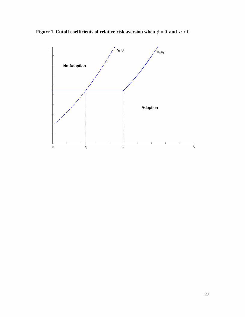
Figure 1 plots the cutoff coefficient of relative risk aversion TUσ and TIσ as a
function of income in the low state LY assuming that 0=φ and 0>ρ . For a given LY ,
if TUσσ < ( TUσσ > ), the farmer would prefer (not) to adopt the hybrid seeds if offered
the uninsured loan. Analogously, if TIσσ < ( TIσσ > ), the farmer would prefer (not) to
adopt the hybrid seeds if offered the insured loan.
Notice that when RYL < , the farmer consumes W regardless of LY which is
seized by the bank due to limited liability and so the cutoff )( LTU Yσ is constant because
9
it does not depend on LY . If, more generally, the bank can seize assets W with probability
0>φ , then consumption in the low state does depend on LY , because
WRYc LL +−= with probability φ . (With probability 1 φ− , consumption in the low state
is Lc W= ). When 0>φ , the cutoff coefficient of relative risk aversion )( LTU Yσ will be
increasing in LY with a slope proportional to 0>φ . Notice also that )( LTI Yσ is
increasing in LY through equation (3) even if 0=φ . When the insured loan is taken,
consumption in the low state if the insurance pays out is given by WYc LL += , which
clearly depends positively on LY . The intuition here is that the higher the level of YL, the
higher the farmer’s default cost (the more the farmer “stands to lose” upon default via
confiscation of his or her output), and so the more valuable is an insured loan.
We are now interested in determining under what conditions a farmer will prefer
the insured loan to the uninsured one. In other words, when will TUTI σσ > ? Figure 1
shows that there is a threshold level RYL <ˆ such that if LL YY ˆ< , then TUTI σσ < , and
TUTI σσ ≥ if LL YY ˆ≥ . Therefore, if income in the low state is low enough, the uninsured
loan contract is already providing enough implicit insurance. Thus some farmers would
adopt the hybrid seeds if offered the uninsured loan, but would prefer to grow the
traditional seeds if offered the insured loan since explicit insurance is too expensive
relative to its value.
In sum, Figure 1 shows that there are situations in which more farmers would
adopt the hybrid seeds with an uninsured loan than with an insured one. Limited liability
turns out to be a key factor in limiting the value of the insurance policy.
3. Experimental Design and Survey Data
The experiment was carried out as a collaborative effort among several partners:
the National Smallholder Farmers Association of Malawi (NASFAM), Opportunity
International Bank of Malawi (OIBM), the Malawi Rural Finance Corporation (MRFC),
the Insurance Association of Malawi (IAM), and the Commodity Risk Management
Group (CRMG) of the World Bank. NASFAM is an NGO that provides technical
10
assistance and marketing services to nearly 100,000 farmers in Malawi. It is by far the
largest farmer association in the country. The farmers in the study were current
NASFAM members. NASFAM field officers disseminated the information on the insured
and uninsured loans to farmers, and handled the logistics of supplying farmers with the
hybrid seeds purchased on credit. OIBM and MRFC are microfinance lenders and
provided the credit for purchase of the hybrid seeds. OIBM is a member of the global
Opportunity International network of microfinance institutions, while MRFC is a
government-owned corporation. IAM designed and underwrote the actual insurance
policies with technical assistance from the World Bank.
The microfinance institutions offered the loans for the hybrid seeds as group
liability contracts for clubs of 10-20 farmers. Take-up of the loan was an individual
decision, but the subset of farmers who took up the loan were told that they were jointly
liable for each others’ loans. In practice, however, joint liability schemes in Malawi are
seldom enforced. When a default occurs, lenders may at best seize the defaulter’s
movable assets, such as furniture or a TV set, but even this happens only rarely.13
NASFAM contacted clubs in June and July 2006 and offered them the opportunity to be
included in the study. Our study sample consists of 159 clubs from four different regions
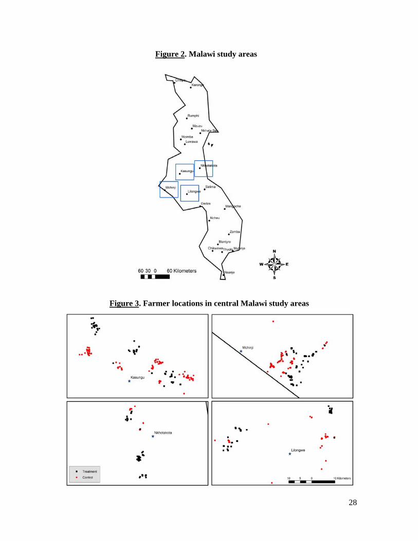
of central Malawi: Lilongwe North, Mchinji, Kasungu, and Nkhotakota. Figure 2 shows
the study locations. In these clubs there were 787 farmers who agreed to be part of the
study and were available to be surveyed in the following September.
To minimize concerns about fairness if farmers discovered that other farmers in
the study were being treated differently, the treatments were randomized at the level of
32 localities. Each locality has roughly 5 clubs from neighboring villages. Localities were
randomized into two equal sized groups: 16 “uninsured” (control) localities and 16
insured (treatment) localities. Figure 3 plots the location of control (in red) and treatment
(in black) farmers. The 394 farmers from “uninsured” localities were simply offered a
loan (standard debt contract) for the hybrid seeds, while the 393 farmers from “insured”
localities were not only offered the loan for the hybrid seeds (identical to the “uninsured”
one) but they also received a rainfall insurance policy with an approximately actuarially-
13 In focus groups with farmers, few suggested having heard stories about someone they did not know having lost his assets after defaulting on a loan, but they all knew defaulters first-hand and none had their assets seized.

11
fair premium. In this insured loan group, farmers were required to take the insurance if
they wanted the loan package.
Farmers were given the option to purchase an improved groundnut only or
improved groundnut and a hybrid maize seed and fertilizer package.14 In order to obtain
either package, a deposit of 12.5 percent of the package amount was required in advance.
The uninsured groundnut loan package provided enough seed (32 kg.) of an improved
variety (ICGV-SM 90704) for planting on one acre of land, with a total of MK 4,692.00
to be repaid at harvest time 10 months later (roughly US$33.51).15 Of this total
repayment, MK 3,680 was the cost of seed and MK 1,012.00 was interest.16 Farmers
offered the insured groundnut package were in addition charged for the insurance
premium, which ranged from MK 297.98 in Nkhotahota to MK 529.77 in Lilongwe
(about 6 to 10 percent of the uninsured principal) so that the total repayment due at
harvest time was between MK 5,130.07 and MK 5,367.45 (roughly US$36.23-
US$38.34). In field trials, the improved groundnut variety performed better than
traditional varieties along several dimensions. It had higher yields, was less susceptible to
drought, had a shorter maturation period, exhibited greater disease resistance, and had
higher oil content.
Corresponding costs for the hybrid maize package (which provided inputs
sufficient for ½ acre of land) were as follows: MK 3,900 for seeds and fertilizer for a
total uninsured package of MK 4,972.50 (US$35.52) and an insurance premium that
ranged from MK647.16 to MK 1,082.29, depending on the reference weather station.
Like the improved groundnut seed, hybrid maize is bred to be disease resistant and high-
yielding. In pre-release trials in mid-altitude areas of Malawi, DK 8051 had higher yield
than all comparison varieties. It outperformed the trial mean by 12.7 percent, and
outperformed MH18, another hybrid variety used by farmers in our sample, by 32.7
14 The option of a maize seed and fertilizer only was not given because maize is typically for consumption, and thus NASFAM and the lenders wanted to ensure repayment of the loan using the proceeds from the sale of groundnut, a cash crop. 15 In October 2006, roughly 140 Malawi kwacha (MK) were convertible to US$1. 16 The annual interest rate for loans in this study was 33%, but because the loan was over a 10-month period, the rate charged was 27.5% (33% x 10 / 12).

12
percent. The DK8051 is also resistant to common diseases including GLS, leaf blight,
and other conditions (Wessels 2001).17
Output on farms planted with hybrid varieties of seeds is still sensitive to rainfall
(Mwale et al 2006, Nigam et al 2006), which potentially makes weather insurance
worthwhile for the hybrid seeds. The insurance policy bundled with the loan pays out a
proportion (or the totality) of the principal and interest depending on the level of rainfall.
In other words, the insured loan is in essence a contingent loan whose repayment amount
depends on the realization of rainfall at the nearest weather station. The coverage for both
maize and groundnut policies is for the rainy season, which is the prime cropping season,
running from September to March. The contract divides the cropping season into three
phases (sowing, podding/flowering and harvest) and pays out if rainfall levels fall below
particular threshold or “trigger” values during each phase. As Figure 4 shows for a given
phase, an upper and lower threshold is specified for each of the three phases. If
accumulated rainfall exceeds the upper threshold, the policy pays zero for that phase.
Otherwise, the policy pays a fixed amount for each millimeter of rainfall below the
threshold, until the lower threshold is reached. If rainfall falls below the lower threshold,
the policy pays a fixed, higher payout. The total payout for the cropping season is then
simply the sum of payouts across the three phases. The maximum payout corresponds to
the total loan amount plus the premium and the interest payment.
The timing of the phases, thresholds and other parameters of the model were
determined using crop models specific to improved groundnut and hybrid maize as well
as interactions with individual farmers. During the baseline survey, when farmers were
asked what affects groundnut production the most, close to 70 percent said rainfall, and
less than 20 percent said pests, the next reason in importance. The upper threshold
corresponds to the crop’s water requirement or the average accumulated rainfall at the
rainfall gauge (whichever is lowest), while the second trigger is intended to capture the
water requirement necessary to avoid complete harvest failure. Translated into financial
market terminology, the relationship between rainfall and payoffs resembles a “put
spread” option for each phase.
17 Although the improved seeds appear less risky in field trials, farmers may not necessarily know this, or may require a period of learning about appropriate farming techniques before being able to realize such improvements. So in the short run the improved seeds may still be more risky.
13
The weather insurance policy was customized to each of the four project regions.
Payouts were based on the rainfall readings at the closest weather station to the individual
in question (there was a separate station for Lilongwe North, Kasungu, Nkhotakota, and
Mchinji). The insurance policy was priced at the actuarially fair premium,18 plus a 17.5%
government-mandated surtax.19 Therefore the premium was lower in places where the
likelihood of a bad rainfall shock is lower.20
All farmers in the study were administered a household socioeconomic survey in
September 2006. The survey covered income, education, assets, income-generating
activities (including detailed information on crop production and crop choice), measures
of risk aversion, and knowledge about financial products such as credit and insurance.
After the completion of the survey, an orientation meeting was held in each of the
32 localities in October 2006 where NASFAM field officers explained the loan product
being offered (insured or uninsured) to the study farmers. Farmers then had two weeks to
decide whether to take up the loan, which required a deposit of 12.5% of the loan amount
at the local NASFAM field office. Seeds and fertilizer were then delivered to pre-
specified collection points near the club meeting place, and planting occurred with the
beginning of the rains in November.
Summary statistics from the baseline survey are presented in Table 1, and variable
definitions are provided in the Appendix.
4. Empirical results
18 To be clear, computing the actuarially fair premium on the insurance policy is straightforward, because payouts depend solely on the occurrence of well-defined meteorological events. Historical data from the same weather stations that are used to determine payouts provide the probability distribution of the weather events. The actuarially fair premium is then simply the expected payout of the policy given the historical distribution of the weather events. 19 The policy was designed by the Insurance Association of Malawi with the technical assistance from the World Bank. Because the World Bank was also involved in the design of the stand-alone weather insurance policies in India, they share a very similar design. The introduction of weather insurance in India is studied in Giné, Townsend and Vickery (2008) and Cole, Topalova and Tobacman (2008). 20 If borrowers did not value insurance, then one should expect take-up of the insured loan to be higher in areas with lower premiums. If, on the contrary, borrowers valued insurance, then the demand for insurance would be correlated with the occurrence of the insured event, and therefore higher demand would be associated with higher premiums, in which case the correlation would be zero. We tested whether take-up was higher in areas with lower premiums and found that while point estimates are in the expected direction (higher take-up with lower premiums), the limited amount of variation in premiums leads to large standard errors so that we cannot reject the null that premiums are unrelated with take-up (results available from authors on request).

14
In what follows, the “treatment group” refers to farmers who were offered the
insured loan, and the “control group” refers to farmers offered the uninsured loan.
Randomization of treatment should ensure that treatment and control groups have similar
baseline characteristics on average. To check this, Table 2 presents means of several key
farmer and household characteristics for the treatment and control groups, as well as the
p-value of the F-test that the difference in means is statistically significantly different
from zero.
For nearly all the variables presented (gender of the respondent, female headship
of the respondent’s household, self-reported risk aversion, respondent’s age, land
ownership, an index of housing quality constructed from indicators for various household
amenities, and net income), the difference in means is not statistically different from zero.
The sole exception is that years of education among treatment group respondents is 0.84
years lower than in the control group, and this difference is statistically significant at the
10% level. As farmer years of education is a key variable (and will later be shown to be
positively correlated with take-up), this is unfortunate. However, we will provide
evidence later that lower education in the treatment group can only go a very small way
towards explaining their lower take-up rates. We also take comfort in the fact that we
cannot reject the hypothesis that all the variables are jointly insignificant in predicting
treatment status (the F-test yields a p-value of 0.31).
Because the treatment is assigned randomly at the locality level, the impact of the
treatment on take-up of the hybrid seed loan can be estimated via the following
regression equation:
(1) Yij = α + βIj + δXij + φj + εij,
where Yij = adoption decision for individual i in locality j (1 if adopting and 0 otherwise),
Ij is insurance status (1 if the loan is insured and 0 otherwise), Xij are individual-level
baseline control variables, and φj are fixed effects for four study regions. εij is a mean-
zero error term. Treatment assignment at the locality level creates spatial correlation
among farmers within the same locality, so we report standard errors that are clustered at
15
the locality level (Moulton 1986). There is a concern that significance tests based on
clustered standard errors may overreject the null when the number of clusters is “small”
(Bertrand, Duflo and Mullainathan 2004; Cameron, Gelbach, and Miller 2008).21
Therefore, we also report p-values derived from a bootstrapping procedure that Cameron,
Gelbach, and Miller (2007) have demonstrated has good size properties with small
numbers of clusters (as few as 5).22
The coefficient β on the insurance dummy variable is the impact of being offered
the insured loan on adoption, and answers the question “How much does insurance raise
demand for the hybrid seed loan?” Due to the randomization of treatment, controls for
baseline variables should not strictly be necessary, and in practice have little effect on the
estimated treatment effect β, but they do help absorb residual variation and reduce
standard errors. In addition, it is useful to include a control for farmer education because,
as discussed above, the locality-level randomization failed to eliminate statistically
significant (at the 10% level) differences between the education levels of treatment and
control respondents.
Table 3 presents estimates of regression equation (1) in specifications with
various combinations of baseline control variables. Column 1 presents the simplest
possible specification, where the only right hand side variable is the indicator for
treatment. The treatment effect (-0.154) is negative and large in magnitude, although the
coefficient is not statistically significantly different from zero at conventional levels (the
p-value implied by clustered standard errors is 0.155, and the bootstrapped p-value is
0.198).
Additional control variables for baseline characteristics in subsequent columns
add explanatory power to the regression (as reflected in rising R-squared) and so help
21 To be sure, it is not clear that 32 should be considered a “small” number of clusters. In Cameron, Gelbach, and Miller (2008), clustered standard errors perform quite well for the 30-cluster case, and Bertrand, Duflo and Mullainathan (2004) find in their CPS application that clustered standard errors do not lead to overrejection of the null hypothesis for as few as 20 clusters (see their Table 8). 22 The bootstrap procedure resamples residuals using so-called Rademacher weights (equal probabilities for 1 or -1) to obtain a new sampling of residuals from a restricted regression that imposes the null hypothesis in each of 999 replications. In each pseudo-sample, the Wald test statistic from OLS estimation with clustered standard errors is calculated for the statistical significance of the coefficient on “Treatment” being different from the null. The location of the original Wald test statistic in the distribution of bootstrapped Wald test statistics provides the bootstrapped p-value.

16
reduce the standard error on the treatment coefficient while having minimal effects on the
coefficient point estimate. Column 2 adds fixed effects for the four study regions, which
reduces the magnitude of the point estimate slightly (to -0.141). The coefficient is now
statistically significant at the 10% level with clustered p-values, and is marginally
significant (p-value 0.116) with bootstrapping.
In column 3, a variety of other control variables are additionally included in the
regression (gender of the respondent, female headship of the respondent’s household,
household income, respondent’s education, respondent’s age, acres of land ownership, an
index of housing quality and net income). The coefficient declines slightly to -0.132 as a
result, and with both types of p-values the coefficient is only marginally significant
(clustered and bootstrapped p-values are 0.107 and 0.140, respectively).
Column 4 allows for more flexible functional forms for the continuous baseline
control variables (respondent’s education, household income, respondent’s age, land
ownership) by including dummy variables for each quintile of these variables. The
coefficient estimate is now -0.128 and it has become slightly more precise. With
clustered standard errors the p-value is 0.082, and with bootstrapping it is 0.120.
Finally, because treatment farmers are less educated on average than control
farmers, it is important to understand whether the control for respondent’s years of
education makes a substantial difference in the estimated coefficient. In column 5, the
dummy variables for education are dropped from the regression. As it turns out, dropping
these controls has very little effect: the coefficient and significance levels are very similar
to those in the previous column where the education dummy variables are included.
Given the marginal or close-to-marginal significance levels, Table 3’s results are
at best suggestive evidence that bundling insurance with the hybrid seed loan led to lower
take-up (by roughly 13 percentage points) compared to the uninsured loan. Having said
that, it is also of interest to test whether we can reject null hypotheses representing
modest positive increases in take-up, such as β = 0.05 or β = 0.10 (increases of 5 and 10
percentage points, respectively).
Table 4 presents clustered and bootstrapped p-values from F-tests of the statistical
significance of the coefficient on Treatment vis-à-vis the null hypotheses β = 0.05 and β
17
= 0.10. Across columns of Table 4, the coefficient on Treatment that is tested is from the
corresponding regression of Table 3.
The null of 0.05 is rejected across all regressions at conventional levels. As
expected, bootstrapped p-values are higher than clustered ones, but even for bootstrapped
p-values the 0.05 null is rejected at significance levels of either 10% (regressions 1-3) or
5% (regressions 4 and 5). The 0.10 null is of course rejected even more strongly,
achieving the 5% significance level in all regressions for bootstrapped p-values (and
achieving the 1% level for clustered standard errors in 4 out of 5 regressions).
In sum, we can reject at conventional significance levels the hypothesis that
bundling weather insurance with the hybrid seed loan led to an increase in take-up of 5
percentage points or more (which, compared to the 33% take-up rate in the control group,
would have been an effect of only modest magnitude).
These results are consistent with the theoretical model of Section 2, which
predicts that if output in the low state (YL) is low enough, fewer farmers will take up the
loan package if it is insured than if it is not insured. This is possible because for low
enough YL, limited liability binds and farmers’ consumption cannot fall below W. The
loan contract provides enough implicit insurance and thus farmers have little interest in
explicit weather insurance – and in fact will exhibit lower demand for a loan bundled
with insurance for which a premium must be paid.
If farmers indeed placed zero value on the insurance, then the lower demand for
insured loan take-up could simply reflect the fact that the insured loan had an effectively
higher interest rate (due to the insurance premium charged). Compared with the annual
interest for the uninsured loan (27.5%), effective interest rates on the insured loan for a
farmer who did not value the insurance were substantially higher (but varied according to
location because of differing probabilities of the rainfall events). Such a farmer taking out
an insured groundnut loan faced an effective interest rate ranging from 37.8% to 44.4%,
depending on the area. This represents an increase in the effective interest rate due to the
insurance premium of from 37.5% at the low end to 61.3% at the high end. Comparing
this to the 39.4% decline in take up associated with the insured loan (13 percentage points
18
off the base of 33.0%), this would imply an interest rate elasticity of credit demand
ranging from 0.64 to 1.05.23
5. Determinants of take-up of insured and uninsured loans
The theoretical model presented in Section 2 also makes testable predictions
regarding the characteristics of farmers that should predict take-up for farmers offered the
insured and uninsured loans. In Figure 1, starting from low levels of low-state income
(YL), increases in YL initially have no relationship with adoption of the uninsured loan
because the risk-aversion coefficient cutoff is flat until YL = R (for YL < R, the bank
confiscates income up to the loan repayment amount R and so there is no variation in
income in the low state, since 0=φ ). However, for the insured loan, an increase in low-
state income should lead to higher take-up. In Figure 1, the risk-aversion coefficient
cutoff line (the dotted line) slopes upward: as YL rises, the risk-aversion cutoff for
adoption rises, and so more individuals in the population choose to adopt.
A sensible empirical test would be to regress the take-up indicator on a measure
of YL, separately for the treatment (insured loan) and control (uninsured loan) groups.
Because no measure of YL is available, instead we examine independent variables related
to the farmer’s education, income, and wealth. This requires an assumption that farmers
with higher education, income, or wealth also have higher income in the low state,
perhaps because they are more likely to follow risk-reducing farming practices (they may
be more likely to have made irrigation investments, may have better knowledge about
avoiding low output realizations, etc.).
Table 5 presents coefficient estimates from such regressions, separately for
farmers in the two different treatment conditions. Columns 1 to 6 are regressions for the
treatment (insured loan) group, and columns 7 to 12 are for the control (uninsured loan)
group. All regressions in the table include region fixed effects plus a constant.
The regressions for the treatment group indicate a positive relationship between
take-up on the one hand, and farmer education, income, and wealth on the other. In 23 These elasticities are not out of line with the one existing randomized study we are aware of on the interest rate elasticity of credit demand. Karlan and Zinman (forthcoming) find that interest rate increases exhibit an interest rate elasticity of greater than 1 in urban South Africa.

19
columns 1 to 4, the take-up indicator is regressed separately on (respectively) the
respondent’s years of schooling, net income, house quality, and acres of land owned. In
each regression the coefficient is positive, and the coefficient on years of schooling is
statistically significantly different from zero at the 5% level. The coefficients on net
income and house quality are marginally significant. In column 6, all four of these
variables are included on the right-hand side, and an F-test of the joint significance of the
coefficients on these four independent variables rejects the null that they are jointly
statistically insignificant with a p-value of 0.03.
By contrast, there is no indication that farmer education, income, and wealth is
related with loan take-up in the control group. In the corresponding regressions for the
control group in columns 7-10, none of the four variables of interest are even marginally
statistically significantly different from zero, and the F-test of the joint significance of the
coefficients on these four variables does not reject the null that they are jointly
statistically insignificant (the p-value is 0.98).
If farmer education, income, and wealth are plausible proxies for low state income
(YL), and if farmers in the study can plausibly be thought to be in the region of Figure 1
where low-state income is low enough (below the repayment amount R), these results are
consistent with the model’s predictions: loan take-up will be uncorrelated with YL when
farmers are offered the uninsured loan, and positively correlated when farmers are
offered the insured loan.
Another result of interest in Table 5 is that take up of the uninsured loan is
negatively associated with farmers’ self-reported risk aversion. In columns 11 and 12, the
coefficient on risk tolerance (-0.015) is negative and statistically significantly different
from zero at the 1% level. A one-point increase in self-reported risk aversion (on a scale
of 0-10) leads to a 1.5 percentage point decrease in the likelihood of taking up the
uninsured loan. The relationship between self-reported risk aversion and take-up is also
negative for farmers offered the insured loan, although the coefficient is smaller in
magnitude (-0.008) and is not statistically significantly different from zero. These results
are consistent with the theoretical model: individuals with higher risk aversion (for given
YL) are more likely to be located above the risk aversion cutoff line in Figure 1 and to
decide not to take up the loan.
20
6. Other potential explanations for take-up differences
It is useful at this point to address other potential explanations for the difference
in take-up across the treatment and control groups.
Given that education is positively correlated with take-up of the insured loan, a
valid concern is that some part of the observed difference in take-up between the
treatment and control groups may be due to the fact that the treatment group had 0.841
fewer years of education on average than the control group (see Table 2). The coefficient
on education in column 6 of Table 5 indicates that this difference in average years of
education should account for roughly 0.0093 (0.93 percentage points) of the take-up
difference between the two groups—a measurable amount, but not nearly enough to
explain the full take-up difference of roughly 13 percentage points.
It is also possible that farmers may have been uncertain about the risk
characteristics of the hybrid seeds, and took the fact that they were offered insurance as a
signal from NASFAM that the seeds were riskier than they would have thought
otherwise. Lower take-up of the credit plus insurance product would then be a rational
response.
Basis risk may also have been a problem: the insurance policy may simply have
been designed in such a way that it was not attractive to farmers because it insured
weather events that had little to do with actual output on the farm. This may have been
the case if the weather stations are too far away (so that rainfall at the weather station is
poorly correlated with rainfall on the farmer’s field), or if the insured meteorological
events are poorly chosen (e.g., rainfall is insured in months that are not important for
output). If basis risk is large enough, then the insurance policy will be unattractive to
farmers and our finding that take-up of the package is lower with insurance (for which
the premium is charged) would not be surprising.
An additional possible explanation is that farmers could have perceived the
default costs as different across the two products. When offered the uninsured loan,
farmers may have thought that with some positive probability NASFAM would not
actually impose substantial penalties if they defaulted on the loan. When the insured loan

21
was offered to farmers, by contrast, there could have been greater emphasis on the fact
that the lender was going to impose penalties for nonpayment (even if the loan were to be
forgiven in the event of poor rainfall). Farmers could therefore have perceived higher
costs for default in the credit plus insurance product, leading that product to have lower
take-up.
7. Conclusion
A large body of theory and empirical work in development economics argues that
technology adoption (and income-maximizing production choices more generally) may
be hindered when returns are risky and insurance or other financial markets are imperfect.
This paper reports the results of an experimental study that tested whether reducing risk
induces greater demand for loans to finance technology adoption. Nearly 800 maize and
groundnut farmers in Malawi (where by far the dominant source of production risk is the
level of rainfall) were offered credit to purchase high-yielding hybrid maize and
groundnut seeds in advance of the planting season. Farmers were randomized into two
groups that differed in whether the loan was insured against poor rainfall. Take-up was
33.0% for farmers who were offered the uninsured loan. Take up was lower, by 13
percentage points, among farmers offered insurance with the loan.
A potential explanation is that farmers already are implicitly insured by the
limited liability inherent in the loan contract, so that bundling a loan with formal
insurance (for which an insurance premium is charged) is effectively an increase in the
interest rate on the loan. We offer suggestive evidence in support of this hypothesis:
among farmers offered the insured loan, take-up is positively associated with a farmer’s
education, income, and wealth. These variables may proxy for the farmer’s default costs
(the value of harvest proceeds that could be seized by the lender), and if so should be
correlated with the benefit a farmer can expect from insurance. By contrast, for farmers
offered the uninsured loan, these characteristics are not associated with take-up.
These results help underscore the difficulties inherent in designing effective approaches
to reducing the consequences of environmental risks for farmers so as to encourage
adoption of income-raising technologies.
22
The focus here has been on the farmer’s demand for insurance, not the lender’s.
When one takes into account the lender’s perspective, a much clearer picture emerges.
For the lender, weather insurance is likely to be an attractive way to mitigate default risk
and thus, it can become an effective risk management tool with the potential of increasing
access to credit in agriculture at lower prices.
Appendix: Variable definitions
Data are from the Malawi Technology Adoption and Risk Initiative (MTARI) farm household survey in September-October 2006. All variables refer to respondent or respondent's household.
Take-up equal to 1 if respondent signed up for hybrid seed loan, 0 otherwise. Treatment equal to 1 if respondent offered insured loan, 0 if offered uninsured loan.
House quality is the first principal component of several binary asset variables. Variables are defined for housing construction materials, water source, and electricity source. In general, variables are defined such that “1” represents a higher standard of living than “0.” The binary asset variables used in this analysis are for brick housing construction, non-earthen floors, metal roofs, and running water (including water piped into the residence and water from a public tap). Additionally, we use two variables that are exceptions to the rule of “1” representing a higher standard of living. The first of these is for well water, as opposed to either running water or unimproved water sources. The second is for gas lighting, as opposed to either electricity or solar power, or firewood, candles, or no lighting.
Net income is computed as the sum of farm profits and non farm income, and is reported in Malawi kwachas (MK). Farm profits are the monetary value of crops produced less the monetary cost of farming inputs. Farming inputs include irrigation, fertilizer, chemical insecticides, manure or animal penning, hired equipment such as tractors, and hired manual labor and oxen labor. Information on farm revenue and expenditure was collected for each plot; total farm profits are computed as the sum of profits over all plots farmed by an individual. Non farm income includes wages from agricultural labor (on other peoples’ farms); wages from non-agricultural labor; wages or in-kind wages from public works programs; remittances; benefits from government programs; pension income; and other sources of income. Information on these sources of income was collected for each respondent, and added to farm profits to compute total net income.
Land owned is in acres. Risk aversion is self-reported on 0-10 scale: higher indicates greater aversion to
risk in trying new crop varieties. Binary variables were generated to allow flexible functional form estimates of the
impact of education, net income and land ownership and are computed as follows. For education, the first quintile includes those with 0 to 2 years of schooling; the second quintile includes those with 3 or 4 years of schooling; the third quintile includes those with 5, 6, or 7 years of schooling; the fourth quintile includes those with 8 years of schooling; and the fifth quintile includes those with 9 to 15 years of schooling. For

23
income, the quintile breakdown is as follows: the first quintile includes those with net incomes of between -215,343 MK and 550 MK; the second quintile includes those with net incomes between 600 MK and 5,380 MK; the third quintile includes those with incomes between 5,400 MK and 13,000 MK; the fourth quintile includes those with incomes between 13,218 MK and 27,300 MK; and the fifth quintile includes those with incomes between 27,500 MK and 3,712,300 MK. Finally, five dummy variables for land ownership represent holdings of 0 to 3 acres; 3.25 to 4 acres; 4.25 to 6 acres; 6.25 to 10 acres; and 10.25 to 108 acres, respectively. Indicator variables for age are binary variables for the following age categories: under age 25, 25-29, 30-34, 35-39, 40-44, 45-49, 50-54, 55-59, 60-60, and 65 and over.
References
Benjamin, Dwayne (1992). “Household Composition, Labor Markets, and Labor Demand: Testing for Separation in Agricultural Household Models” Econometrica, Vol. 60, No. 2, pp. 287-322. Bertrand, M., E. Duflo and S. Mullainathan (2004). “How Much Should We Trust Differences-in-Differences Estimates?” Quarterly Journal of Economics, Vol. 119, pp. 249-275. Besley, Timothy and Anne Case (1993). “Modeling Technology Adoption in Developing Countries.” American Economic Association Paper and Proceedings, Vol. 83, No. 2, May, pp. 396-402. Besley, Timothy and Anne Case (1994). “Diffusion as a Learning Process: Evidence from HYV Cotton,” Princeton University Working Paper. Binswanger, Hans P. and Donald A. Sillers (1983). "Risk Aversion and Credit Constraints in Farmers' Decision-Making: A Reinterpretation." Journal of Development Studies, Vol. 20, 5-21. Boucher, Stephen, Michael R. Carter, Catherine Guirkinger (2008). “Risk Rationing and wealth Effects in Credit Markets.” American Journal of Agricultural Economics, Vol. 90, No. 2, May, pp. 409-423. Chaudhuri, Shubham and Theresa Osborne (2002). “Financial Market Imperfections and Technical Change in a Poor Agrarian Economy” Working Paper, European University Institute, Florence, Italy. Cameron, A. Colin, Jonah B. Gelbach, and Doug Miller (2008). “Bootstrap-Based Improvements for Inference with Clustered Errors,” Review of Economics and Statistics, Vol. 90, No. 3, August, pp. 414-427.
24
Cole, Shawn, Xavier Giné, Jeremy Tobacman, Robert Townsend, Petia Topalova and James Vickery 2008, “Barriers to Household Risk Management” working paper, Harvard Business School, World Bank, Oxford University, MIT, NY Fed and IMF. Conley, Timothy and Christopher Udry, “Learning About a New Technology: Pineapple in Ghana,” mimeo, Yale University, July 2005. Conning, Jonathan and Christopher Udry (2005). “Rural Financial Markets in Developing Countries,” in R. E. Everson, P. Pingali, and T.P. Schultz (eds.), The Handbook of Agricultural Economics, Vol. 3: Farmers, Farm Production, and Farm Markets, Elsevier Science. Dercon, Stefan and Luc Christiaensen, “Consumption risk, technology adoption and poverty traps: evidence from Ethiopia,” World Bank Policy Research Working Paper 4257, June 2007. Dowd, Kevin, 1992. “Optimal Financial Contracts” Oxford Economic Papers 44, pp. 672-693. Duflo, Esther, Michael Kremer and Jonathan Robinson, “Understanding Technology Adoption: Fertilizer in Western Kenya: Evidence from Field Experiments,” mimeo, MIT and Harvard University, April 2006. Evenson, Robert (1974). “International Diffusion of Agrarian Technology.” Journal of Economic History, Vol. 34(1), March, pp. 51-73. Evenson, R. and L. Westphal (1995). “Technological Change and Technology Strategy.” Handbook of Development Economics. J. Behrman and T. N. Srinivasan. Amsterdam, North-Holland. 3A: 2209-2300. Feder, Gershon & Just, Richard E & Zilberman, David, 1985. "Adoption of Agricultural Innovations in Developing Countries: A Survey," Economic Development and Cultural Change, University of Chicago Press, vol. 33(2), pp. 255-98. Foster, A. and M. Rosenzweig (1995) “Learning by Doing and Learning from Others: Human Capital and Technical Change in Agriculture” Journal of Political Economy, Vol. 103(6), p 1176-1209. Giné, Xavier, Robert Townsend, and James Vickery (2008), “Patterns of Rainfall Insurance Participation in Rural India,” World Bank Economic Review, forthcoming. Ghosh, P., D. Mookherjee, and D. Ray (2000). “Credit Rationing in Developing Countries: An Overview of the Theory,” in D. Mookherjee and D. Ray, eds., Readings in the Theory of Economic Development, Malden, MA: Blackwell, pp. 283-301.
25
Goldman, Abe (1993). “Agricultural Innovation in Three Areas of Kenya: Neo-Boserupian Theories and Regional Characterization.” Economic Geography, Vol. 69(1), January, pp. 44-71. Griliches, Zvi (1957). “Hybrid Corn: An Exploration in the Economics of Technological Change.” Econometrica, Vol. 25(4), October, pp. 501-522. Just, Richard E. and David Zilberman (1983). “Stochastic Structure, Farm Size and Technology Adoption in Developing Agriculture.” Oxford Economic Papers, Vol. 35(2), July, pp. 307-328. Karlan, Dean S., and Jonathan Zinman, “Credit Elasticities in Less-Developed Economies: Implications for Microfinance,” American Economic Review, forthcoming. Moulton, Brent, “Random Group Effects and the Precision of Regression Estimates,” Journal of Econometrics, 32, 3, August 1986, p. 385-397. Munshi, Kaivan, “Technology Diffusion,” in Kaushik Basu, ed., Oxford Companion to Economics in India. New Delhi: Oxford University Press, forthcoming. Munshi, Kaivan, “Social Learning in a Heterogeneous Population: Technology Diffusion in the Indian Green Revolution,” Journal of Development Economics, 73 (1), 2004, pp. 185-215. Mwale, C.D., S.C. Nambuzi, A.E. Kauwa, D.Kamalongo I.Ligowe, V.H. Kabambe and W.Mhango, "On-farm evaluation of drought and low-nitrogen tolerant varieties using the mother-baby scheme in 2005/06 season," working paper, Bunda College of Agriculture, University of Malawi, 2006. Nigam, S. N., R. Aruna, D. Y. Giri, G. V Ranga Rao, and A. G. S. Reddy, Obtaining Sustainable Higher Groundnut Yields: Principles and Practices of Cultivation. Andhra Pradesh, India: International Crop Research Institute for the Semi-Arid Tropics, 2006. Rogers, Everett M., The Diffusion of Innovations, 4th Edition. New York: Simon & Schuster, 1995. Rosenzweig, Mark and Kenneth Wolpin, “Credit Market Constraints, Consumption Smoothing, and the Accumulation of Durable Production Assets in Low-Income Countries: Investments in Bullocks in India,” Journal of Political Economy, Vol. 101, No. 2, 1993, pp. 223-244. Simtowe, Frankin, “Can risk-aversion explain part of the non-adoption puzzle for hybrid maize? Empirical evidence from Malawi,” Journal of Applied Sciences, 6, 7, 2006, p. 1490-1498.
26
Simtowe, Franklin and Manfred Zeller, “The impact of access to credit on the adoption of hybrid maize in Malawi: an empirical test of an agricultural household model under credit market failure,” Munich Personal RePec Archive (MPRA) Paper No. 45, September 2006. Smale, Melinda, Paul W. Heisey, and Howard D. Leathers, “Maize of the Ancestors and Modern Varieties: The Microeconomics of High-Yielding Variety Adoption in Malawi,” Economic Development and Cultural Change, 43, 2, January 1995, p. 351-368. Smale, Melinda and Thom Jayne, “Maize in Eastern and Southern Africa: ‘Seeds’ of Success in Retrospect,” International Food Policy Research Institute, EPTD Discussion Paper No. 97, January 2003. Wessels, W. (2001) “Proposal to Release DK8051 and DK8031 and DK8041”, Monsanto South Africa. World Bank, “Malawi Poverty and Vulnerability Assessment 2006: Investing in Our Future,” draft, June 2006.
27
Figure 1. Cutoff coefficients of relative risk aversion when 0=φ and 0>ρ
28
Figure 2. Malawi study areas
Figure 3. Farmer locations in central Malawi study areas

29
Figure 4. Insurance policy The rainfall insurance policy divides the cropping season into three phases. The graph below shows how rainfall during the phase translates into the insurance payout for one phase.
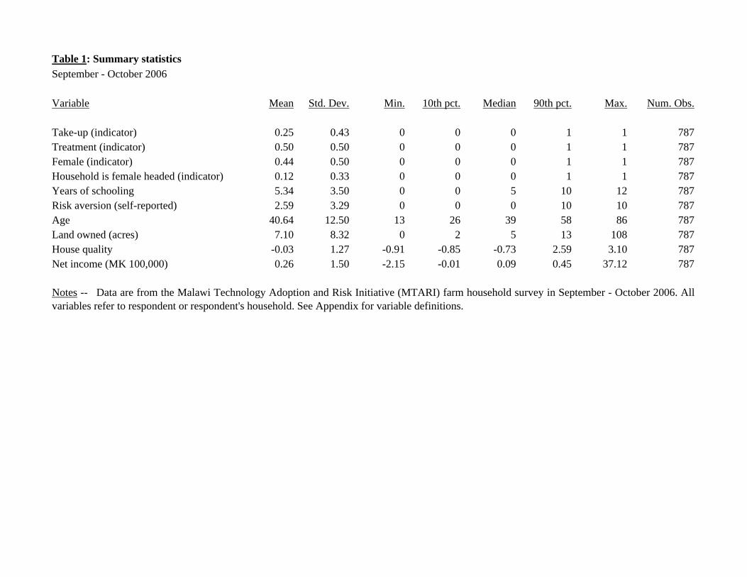
Table 1: Summary statisticsSeptember - October 2006
Variable Mean Std. Dev. Min. 10th pct. Median 90th pct. Max. Num. Obs.
Take-up (indicator) 0.25 0.43 0 0 0 1 1 787Treatment (indicator) 0.50 0.50 0 0 0 1 1 787Female (indicator) 0.44 0.50 0 0 0 1 1 787Household is female headed (indicator) 0.12 0.33 0 0 0 1 1 787Years of schooling 5.34 3.50 0 0 5 10 12 787Risk aversion (self-reported) 2.59 3.29 0 0 0 10 10 787Age 40.64 12.50 13 26 39 58 86 787Land owned (acres) 7.10 8.32 0 2 5 13 108 787House quality -0.03 1.27 -0.91 -0.85 -0.73 2.59 3.10 787Net income (MK 100,000) 0.26 1.50 -2.15 -0.01 0.09 0.45 37.12 787
Notes -- Data are from the Malawi Technology Adoption and Risk Initiative (MTARI) farm household survey in September - October 2006. Allvariables refer to respondent or respondent's household. See Appendix for variable definitions.

Table 2: Differences in means, treatment vs. control groupSeptember - October 2006
Variable Treatment mean
Control mean
Difference p-value
Female (indicator) 0.443 0.445 -0.002 0.975
Household is female headed (indicator) 0.125 0.119 0.006 0.852
Years of schooling 4.919 5.760 -0.841* 0.062
Risk aversion (self-reported) 2.632 2.564 0.068 0.779
Age 40.936 40.357 0.579 0.759
Land owned 6.440 7.759 -1.319 0.117
House quality -0.144 0.087 -0.231 0.228
Net income (MK 100,000) 0.202 0.316 -0.114 0.364
* significant at 10%; ** significant at 5%; *** significant at 1%
Notes -- Table presents means of key variables for treatment group (farmers offered insuredloan) and control group (farmers offered uninsured loan) in September - October 2006, prior totreatment. P-value is for F-test of difference in means across treatment and control groups, andaccounts for clustering at level of 32 localities. See Appendix for variable definitions.
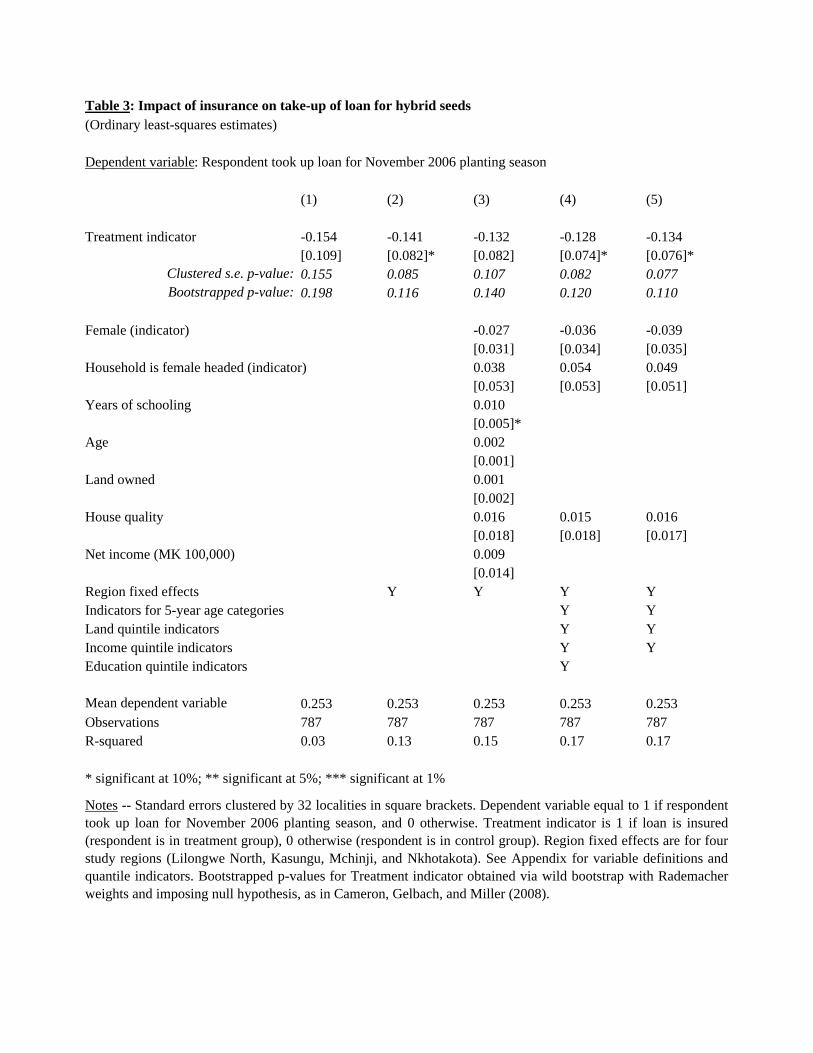
Table 3: Impact of insurance on take-up of loan for hybrid seeds(Ordinary least-squares estimates)
Dependent variable: Respondent took up loan for November 2006 planting season
(1) (2) (3) (4) (5)
Treatment indicator -0.154 -0.141 -0.132 -0.128 -0.134[0.109] [0.082]* [0.082] [0.074]* [0.076]*
Clustered s.e. p-value: 0.155 0.085 0.107 0.082 0.077Bootstrapped p-value: 0.198 0.116 0.140 0.120 0.110
Female (indicator) -0.027 -0.036 -0.039[0.031] [0.034] [0.035]
Household is female headed (indicator) 0.038 0.054 0.049[0.053] [0.053] [0.051]
Years of schooling 0.010[0.005]*
Age 0.002[0.001]
Land owned 0.001[0.002]
House quality 0.016 0.015 0.016[0.018] [0.018] [0.017]
Net income (MK 100,000) 0.009[0.014]
Region fixed effects Y Y Y YIndicators for 5-year age categories Y YLand quintile indicators Y YIncome quintile indicators Y YEducation quintile indicators Y
Mean dependent variable 0.253 0.253 0.253 0.253 0.253Observations 787 787 787 787 787R-squared 0.03 0.13 0.15 0.17 0.17
* significant at 10%; ** significant at 5%; *** significant at 1%
Notes -- Standard errors clustered by 32 localities in square brackets. Dependent variable equal to 1 if respondenttook up loan for November 2006 planting season, and 0 otherwise. Treatment indicator is 1 if loan is insured(respondent is in treatment group), 0 otherwise (respondent is in control group). Region fixed effects are for fourstudy regions (Lilongwe North, Kasungu, Mchinji, and Nkhotakota). See Appendix for variable definitions andquantile indicators. Bootstrapped p-values for Treatment indicator obtained via wild bootstrap with Rademacherweights and imposing null hypothesis, as in Cameron, Gelbach, and Miller (2008).
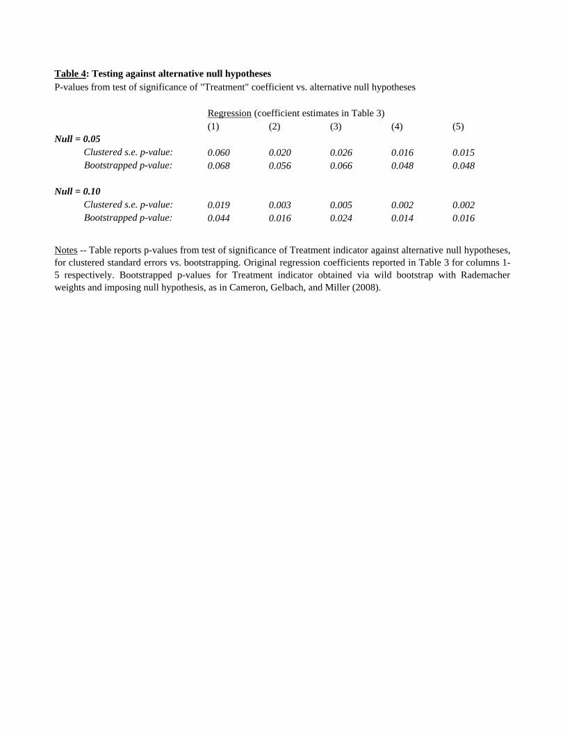
Table 4: Testing against alternative null hypothesesP-values from test of significance of "Treatment" coefficient vs. alternative null hypotheses
Regression (coefficient estimates in Table 3)(1) (2) (3) (4) (5)
Null = 0.05Clustered s.e. p-value: 0.060 0.020 0.026 0.016 0.015Bootstrapped p-value: 0.068 0.056 0.066 0.048 0.048
Null = 0.10Clustered s.e. p-value: 0.019 0.003 0.005 0.002 0.002Bootstrapped p-value: 0.044 0.016 0.024 0.014 0.016
Notes -- Table reports p-values from test of significance of Treatment indicator against alternative null hypotheses,for clustered standard errors vs. bootstrapping. Original regression coefficients reported in Table 3 for columns 1-5 respectively. Bootstrapped p-values for Treatment indicator obtained via wild bootstrap with Rademacherweights and imposing null hypothesis, as in Cameron, Gelbach, and Miller (2008).
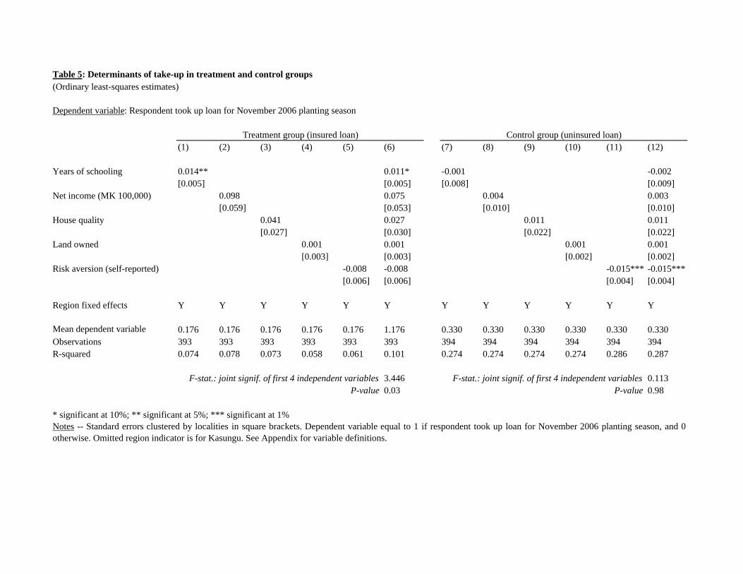
Table 5: Determinants of take-up in treatment and control groups(Ordinary least-squares estimates)
Dependent variable: Respondent took up loan for November 2006 planting season
(1) (2) (3) (4) (5) (6) (7) (8) (9) (10) (11) (12)
Years of schooling 0.014** 0.011* -0.001 -0.002[0.005] [0.005] [0.008] [0.009]
Net income (MK 100,000) 0.098 0.075 0.004 0.003[0.059] [0.053] [0.010] [0.010]
House quality 0.041 0.027 0.011 0.011[0.027] [0.030] [0.022] [0.022]
Land owned 0.001 0.001 0.001 0.001[0.003] [0.003] [0.002] [0.002]
Risk aversion (self-reported) -0.008 -0.008 -0.015*** -0.015***[0.006] [0.006] [0.004] [0.004]
Region fixed effects Y Y Y Y Y Y Y Y Y Y Y Y
Mean dependent variable 0.176 0.176 0.176 0.176 0.176 1.176 0.330 0.330 0.330 0.330 0.330 0.330Observations 393 393 393 393 393 393 394 394 394 394 394 394R-squared 0.074 0.078 0.073 0.058 0.061 0.101 0.274 0.274 0.274 0.274 0.286 0.287
F-stat.: joint signif. of first 4 independent variables 3.446 F-stat.: joint signif. of first 4 independent variables 0.113P-value 0.03 P-value 0.98
* significant at 10%; ** significant at 5%; *** significant at 1%
Treatment group (insured loan) Control group (uninsured loan)
Notes -- Standard errors clustered by localities in square brackets. Dependent variable equal to 1 if respondent took up loan for November 2006 planting season, and 0otherwise. Omitted region indicator is for Kasungu. See Appendix for variable definitions.