Embed Size (px)
Citation preview

Instruments and Data Comparability: A Progress Report
Suchanan Tambunlertchai∗
University of Chicago
September 2009
Project Background
The Townsend Thai Project has been collecting annual household data in four provinces in Thailandsince 1997. In May 1997, the Big Survey spanning four provinces was conducted. These four provinceswere Chachoengsao, Lopburi, Buriram, and Sisaket. The first two are situated in the more fertileCentral region of Thailand, and the latter two in the poorer Northeast region. In each province,12 tambons (sub-districts) were randomly selected. Then, four villages from each tambon werechosen. And finally, from each village, 15 households are chosen, making a total of 2,880 householdsin the sample. The Big Survey compiled detailed information on households, which include data ondemographics, income, consumption, asset, borrowing, lending, and agricultural and entrepreneurialactivities.
The onset of the Asian financial crisis later in 1997 turned the Big Survey dataset into a naturalbenchmark of normal times, which can be compared with the fluctuations to come. In May 1998,therefore, the project was expanded and the Annual Resurvey began. One third of the original BigSurvey sample (4 tambons randomly chosen from the original 12) was chosen for the Annual Resurveygoing forward. The questionnaire for the Resurvey is similar to that used in the Big Survey, but withmost stock variables now changed to flow.
In 1998, monthly household surveys also began. The Monthly Baseline Survey was first conducted inAugust 1998 on 720 households, using a questionnaire similar to that of the Big Survey. From each ofthe four provinces from the Big Survey, one tambon was selected for the Baseline Survey. This tambonwas different from those four chosen for the Annual Resurvey. For the Monthly Baseline Survey, the15 households from each village were augmented with 30 more, making a total of 45 households pervillage. Information from the Baseline Survey was tracked in subsequent monthly interviews. Themonthly questionnaire is different from previous questionnaires used in the Big Survey, the MonthlyBaseline, or the Annual Resurvey. Although the information collected in the Monthly Survey is of thesame nature as that in the Annual Resurvey, it focuses on capturing changing household, agricultural,and business activities at a much greater detail.
So although the Annual Resurvey and the Monthly Survey grew from the same underlying Big Surveysample, they differ in details and track different populations over time. But because the two surveysprovide complementary information, an understanding of the relationship between the two samples
∗I thank Professor Robert M. Townsend for his helpful comments and guidance. All errors are mine. Questions andcomments may be directed to [email protected].
Instruments and Data ComparabilityTambunlertchai
September 2009Page 2
would be valuable for linking these datasets. For some research questions, the Annual data may bemore suitable while for others, the more detailed Monthly data may be needed. To be able to abstractfrom one to use the other with an understanding of how they are related would allow for more completeinsights into any given study.
Scope of the Project
The purpose of this project is precisely to investigate the relationship between the Annual and theMonthly data. The questions of interest include whether or not the two samples differ statisticallyfrom each other, and if so, whether this was due to differences in the underlying households, geography,or questionnaires. As a first step, the time series averages of key variables in the Annual and theMonthly data are compared. Then the statistical mean comparison test was conducted to comparethe two samples. Results from these initial comparisons showed somewhat divergent trends in the twodatasets. This raises concern that the differences may have stemmed from the different questionnairesused for the Annual Resurvey and the Monthly Survey, and the different ways in which some of thevariables are constructed. If the two questionnaires, designed to collect similar information, yielddifferent data from otherwise similar households, a revision of the questionnaires would need to beconsidered. To investigate this possibility, we rely on the subset of the Big Survey sample that wassubsequently used for the Monthly Survey, that is, the 15 original households in each village prior tobeing augmented with 30 additional ones. This subsample has been exposed to both the Annual andthe Monthly questionnaires. If the ways in which variables are constructed affected their values, orif the questionnaires unintentionally elicited inconsistent responses, the transition from the Annual tothe Monthly questionnaire would be apparent in the households’ time series. A close look at thissubsample reveals a smooth transition, giving us comfort in the validity of the questionnaires.
The ensuing sections are organized as follows. The first section discusses findings from the time seriescomparison of the two datasets. Next, results from the mean comparison tests are reported. Thethird section gives an analysis of the Big Survey and Monthly Survey overlap. Finally, the last sectiongives a brief conclusion and discusses next steps.
Time Series Comparison
The project begins with a simple comparison of the time series averages of key variables in the Monthlyand Annual data. This is done to offer some visual gauge of how the two samples have evolved overtime. The comparisons use all available households in the two datasets, including those that reportedzero for some categories. For example, households that reported zero business income are included inthe calculation of the average business income.
To make monetary figures comparable across years, values were converted to 2005 Thai Baht. Nominalvalues were deflated using Headline CPI from the Bank of Thailand. CPI tables are included in theAppendix. Monthly data are aggregated up to annual levels prior to taking sample averages. Itshould be noted that in the Annual Resurvey, interviews are based on a 12-month recall questionnaire.These interviews are typically conducted between April and May of each year, which means that therecall period usually ranges from May of year t − 1 to April of year t when the survey in question isfielded. However, the Monthly data collection began in September 1999. To maximize the use ofavailable data, annualization of the Monthly data is done from September of year t − 1 to August ofyear t. This causes a slight mismatch in the timeframes being compared. But as we shall see, trends

Instruments and Data ComparabilityTambunlertchai
September 2009Page 3
in the two datasets are divergent enough such that it would be diffi cult to explain the differences withslight mismatch in timing.
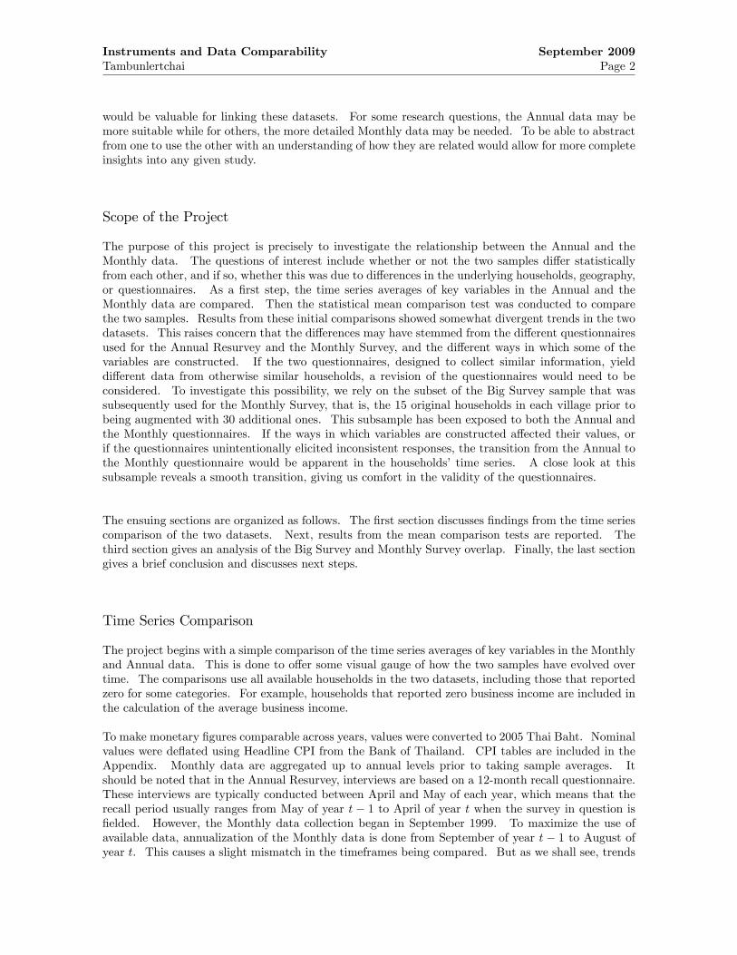
Figure 1 compares Annual and Monthly time series averages for the 4 provinces. Panels on the leftare Annual data, while those on the right are annualized Monthly. Note that Annual panels go from1997 - 2006 while Monthly panels go from 1999 - 2005.

Instruments and Data ComparabilityTambunlertchai
September 2009Page 4
Figure 1a. Revenue Comparisons
Panels on the left are constructed from the Annual data,.
Panels on the right are constructed from annualizing the Monthly data.
0
10,000
20,000
30,000
40,000
50,000
60,000
70,000
80,000
90,000
100,000
1997 1998 1999 2000 2001 2002 2003 2004 2005 2006
2005 Thai Baht
Chachoengsao: Mean Revenue by Source (1997‐2006)
CULTIVATION
LIVESTOCK
LABOR
SHRIMP/FISH
BUSINESS
0
20,000
40,000
60,000
80,000
100,000
120,000
140,000
160,000
180,000
1999 2000 2001 2002 2003 2004 2005
2005 Thai Baht
Chachoengsao: Annualized Mean Revenue by Source (1999‐2005)
CULTIVATION
LIVESTOCK
LABOR
SHRIMP/FISH
BUSINESS
0
10,000
20,000
30,000
40,000
50,000
60,000
70,000
80,000
90,000
1997 1998 1999 2000 2001 2002 2003 2004 2005 2006
2005 Thai Baht
Lopburi: Mean Revenues by Source (19997‐2006)
CULTIVATION
LIVESTOCK
LABOR
SHRIMP/FISH
BUSINESS
0
20,000
40,000
60,000
80,000
100,000
120,000
140,000
1999 2000 2001 2002 2003 2004 2005
2005 Thai Baht
Lopburi: Annualized Mean Revenues by Source (1999‐2005)
CULTIVATION
LIVESTOCK
LABOR
SHRIMP/FISH
BUSINESS
80,000
Buriram: Mean Revenues by Source (1997‐2006) Buriram: Annualized Mean Revenues by Source (1999‐2005)
0
10,000
20,000
30,000
40,000
50,000
60,000
70,000
80,000
90,000
100,000
1997 1998 1999 2000 2001 2002 2003 2004 2005 2006
2005 Thai Baht
Chachoengsao: Mean Revenue by Source (1997‐2006)
CULTIVATION
LIVESTOCK
LABOR
SHRIMP/FISH
BUSINESS
0
20,000
40,000
60,000
80,000
100,000
120,000
140,000
160,000
180,000
1999 2000 2001 2002 2003 2004 2005
2005 Thai Baht
Chachoengsao: Annualized Mean Revenue by Source (1999‐2005)
CULTIVATION
LIVESTOCK
LABOR
SHRIMP/FISH
BUSINESS
0
10,000
20,000
30,000
40,000
50,000
60,000
70,000
80,000
90,000
1997 1998 1999 2000 2001 2002 2003 2004 2005 2006
2005 Thai Baht
Lopburi: Mean Revenues by Source (19997‐2006)
CULTIVATION
LIVESTOCK
LABOR
SHRIMP/FISH
BUSINESS
0
20,000
40,000
60,000
80,000
100,000
120,000
140,000
1999 2000 2001 2002 2003 2004 2005
2005 Thai Baht
Lopburi: Annualized Mean Revenues by Source (1999‐2005)
CULTIVATION
LIVESTOCK
LABOR
SHRIMP/FISH
BUSINESS
0
10,000
20,000
30,000
40,000
50,000
60,000
70,000
80,000
1997 1998 1999 2000 2001 2002 2003 2004 2005 2006
2005 Thai Baht
Buriram: Mean Revenues by Source (1997‐2006)
CULTIVATION
LIVESTOCK
LABOR
SHRIMP/FISH
BUSINESS
0
20,000
40,000
60,000
80,000
100,000
120,000
140,000
160,000
1999 2000 2001 2002 2003 2004 2005
2005 Thai Baht
Buriram: Annualized Mean Revenues by Source (1999‐2005)
CULTIVATION
LIVESTOCK
LABOR
SHRIMP/FISH
BUSINESS
0
20,000
40,000
60,000
80,000
100,000
120,000
140,000
1997 1998 1999 2000 2001 2002 2003 2004 2005 2006
2005 Thai Baht
Sisaket: Revenue by Source (1997‐2006)
CULTIVATION
LIVESTOCK
LABOR
SHRIMP/FISH
BUSINESS
0
10,000
20,000
30,000
40,000
50,000
60,000
1999 2000 2001 2002 2003 2004 2005
2005 Thai Baht
Sisaket: Annualized Revenue by Source (1999‐2005)
CULTIVATION
LIVESTOCK
LABOR
SHRIMP/FISH
BUSINESS

Instruments and Data ComparabilityTambunlertchai
September 2009Page 5
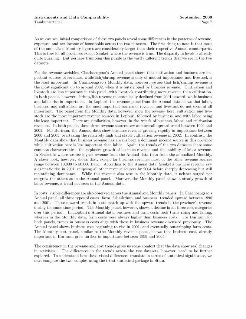
Figure 1b. Expense Comparisons
Panels on the left are constructed from the Annual data,.
Panels on the right are constructed from annualizing the Monthly data.
0
10,000
20,000
30,000
40,000
50,000
60,000
70,000
80,000
90,000
1997 1998 1999 2000 2001 2002 2003 2004 2005 2006
Chachoengsao: Mean Expenses (in 2005 Thai Baht)
FARM
SHRIMP/FISH
BUSINESS
0
20,000
40,000
60,000
80,000
100,000
120,000
1999 2000 2001 2002 2003 2004 2005
Chachoengsao: Annualized Mean Expenses (2005 Thai Baht)
FARM
SHRIMP/FISH
BUSINESS
0
10,000
20,000
30,000
40,000
50,000
60,000
70,000
80,000
90,000
100,000
1997 1998 1999 2000 2001 2002 2003 2004 2005 2006
Lopburi: Mean Expenses (in 2005 Thai Baht)
FARM
SHRIMP/FISH
BUSINESS
0
10,000
20,000
30,000
40,000
50,000
60,000
70,000
80,000
90,000
100,000
1999 2000 2001 2002 2003 2004 2005
Lopburi: Annualized Mean Expenses (2005 Thai Baht)
FARM
SHRIMP/FISH
BUSINESS
60,000
Buriram: Mean Expenses (in 2005 Thai Baht) Buriram: Annualized Mean Expenses (2005 Thai Baht)
0
10,000
20,000
30,000
40,000
50,000
60,000
70,000
80,000
90,000
1997 1998 1999 2000 2001 2002 2003 2004 2005 2006
Chachoengsao: Mean Expenses (in 2005 Thai Baht)
FARM
SHRIMP/FISH
BUSINESS
0
20,000
40,000
60,000
80,000
100,000
120,000
1999 2000 2001 2002 2003 2004 2005
Chachoengsao: Annualized Mean Expenses (2005 Thai Baht)
FARM
SHRIMP/FISH
BUSINESS
0
10,000
20,000
30,000
40,000
50,000
60,000
70,000
80,000
90,000
100,000
1997 1998 1999 2000 2001 2002 2003 2004 2005 2006
Lopburi: Mean Expenses (in 2005 Thai Baht)
FARM
SHRIMP/FISH
BUSINESS
0
10,000
20,000
30,000
40,000
50,000
60,000
70,000
80,000
90,000
100,000
1999 2000 2001 2002 2003 2004 2005
Lopburi: Annualized Mean Expenses (2005 Thai Baht)
FARM
SHRIMP/FISH
BUSINESS
0
10,000
20,000
30,000
40,000
50,000
60,000
1997 1998 1999 2000 2001 2002 2003 2004 2005 2006
Buriram: Mean Expenses (in 2005 Thai Baht)
FARM
SHRIMP/FISH
BUSINESS
0
10,000
20,000
30,000
40,000
50,000
60,000
70,000
80,000
90,000
100,000
1999 2000 2001 2002 2003 2004 2005
Buriram: Annualized Mean Expenses (2005 Thai Baht)
FARM
SHRIMP/FISH
BUSINESS
0
10,000
20,000
30,000
40,000
50,000
60,000
70,000
80,000
90,000
100,000
1997 1998 1999 2000 2001 2002 2003 2004 2005 2006
Sisaket: Mean Expenses (in 2005 Thai Baht)
FARM
SHRIMP/FISH
BUSINESS
0
5,000
10,000
15,000
20,000
25,000
1999 2000 2001 2002 2003 2004 2005
Sisaket: Annualized Mean Expenses (2005 Thai Baht)
FARM
SHRIMP/FISH
BUSINESS

Instruments and Data ComparabilityTambunlertchai
September 2009Page 6
Figure 1c. Net Income Comparisons
Panels on the left are constructed from the Annual data,.
Panels on the right are constructed from annualizing the Monthly data.
‐10,000
0
10,000
20,000
30,000
40,000
50,000
60,000
1997
1998
1999
2000
2001
2002
2003
2004
2005
2006
Chachoengsao: Mean Net Income (2005 TBt)
FARM
SHRIMP/FISH
BUSINESS
LABOR
‐40,000
‐20,000
0
20,000
40,000
60,000
80,000
100,000
120,000
140,000
160,000
1999
2000
2001
2002
2003
2004
2005
Chachoengsao: Annualized Mean Net Income (2005 TBt)
FARM
SHRIMP/FISH
BUSINESS
LABOR
‐20,000
0
20,000
40,000
60,000
80,000
100,000
1997
1998
1999
2000
2001
2002
2003
2004
2005
2006
Lopburi: Mean Net Income (2005 Thai Baht)
FARM
SHRIMP/FISH
BUSINESS
LABOR
0
20,000
40,000
60,000
80,000
100,000
120,000
1999
2000
2001
2002
2003
2004
2005
Lopburi: Mean Net Income by Source (2005 Thai Baht)
FARM
SHRIMP/FISH
BUSINESS
LABOR
50 000
Buriram: Mean Net Income by Source (2005 TBt)
70 000
Buriram: Annualized Mean Net Income (2005 Thai Baht)
‐10,000
0
10,000
20,000
30,000
40,000
50,000
60,000
1997
1998
1999
2000
2001
2002
2003
2004
2005
2006
Chachoengsao: Mean Net Income (2005 TBt)
FARM
SHRIMP/FISH
BUSINESS
LABOR
‐40,000
‐20,000
0
20,000
40,000
60,000
80,000
100,000
120,000
140,000
160,000
1999
2000
2001
2002
2003
2004
2005
Chachoengsao: Annualized Mean Net Income (2005 TBt)
FARM
SHRIMP/FISH
BUSINESS
LABOR
‐20,000
0
20,000
40,000
60,000
80,000
100,000
1997
1998
1999
2000
2001
2002
2003
2004
2005
2006
Lopburi: Mean Net Income (2005 Thai Baht)
FARM
SHRIMP/FISH
BUSINESS
LABOR
0
20,000
40,000
60,000
80,000
100,000
120,000
1999
2000
2001
2002
2003
2004
2005
Lopburi: Mean Net Income by Source (2005 Thai Baht)
FARM
SHRIMP/FISH
BUSINESS
LABOR
‐10,000
0
10,000
20,000
30,000
40,000
50,000
1997
1998
1999
2000
2001
2002
2003
2004
2005
2006
Buriram: Mean Net Income by Source (2005 TBt)
FARM
SHRIMP/FISH
BUSINESS
LABOR
‐20,000
‐10,000
0
10,000
20,000
30,000
40,000
50,000
60,000
70,000
1999
2000
2001
2002
2003
2004
2005
Buriram: Annualized Mean Net Income (2005 Thai Baht)
FARM
SHRIMP/FISH
BUSINESS
LABOR
‐10,000
0
10,000
20,000
30,000
40,000
50,000
60,000
1997
1998
1999
2000
2001
2002
2003
2004
2005
2006
Sisaket: Mean Net Income by Source (2005 Thai Baht)
FARM
SHRIMP/FISH
BUSINESS
LABOR
0
10,000
20,000
30,000
40,000
50,000
60,000
1999
2000
2001
2002
2003
2004
2005
Sisaket: Annualized Mean Net Income (2005 Thai Baht)
FARM
SHRIMP/FISH
BUSINESS
LABOR
Instruments and Data ComparabilityTambunlertchai
September 2009Page 7
As we can see, initial comparisons of these two panels reveal some differences in the patterns of revenue,expenses, and net income of households across the two datasets. The first thing to note is that mostof the annualized Monthly figures are considerably larger than their respective Annual counterparts.This is true for all provinces except Sisaket, where the reverse is true. The disparity in levels is alreadyquite puzzling. But perhaps trumping this puzzle is the vastly different trends that we see in the twodatasets.
For the revenue variables, Chachoengsao’s Annual panel shows that cultivation and business are im-portant sources of revenues, while fish/shrimp revenue is only of modest importance, and livestock isthe least important. In Chachoengsao’s Monthly data, however, we see that fish/shrimp revenue isthe most significant up to around 2002, when it is outstripped by business revenue. Cultivation andlivestock are less important in this panel, with livestock contributing more revenue than cultivation.In both panels, however, shrimp/fish revenue monotonically declined from 2001 onward, while businessand labor rise in importance. In Lopburi, the revenue panel from the Annual data shows that labor,business, and cultivation are the most important sources of revenue, and livestock do not seem at allimportant. The panel from the Monthly data, however, show the reverse—here, cultivation and live-stock are the most important revenue sources in Lopburi, followed by business, and with labor beingthe least important. There are similarities, however, in the trends of business, labor, and cultivationrevenues. In both panels, these three revenue sources saw and overall upward trend between 1999 and2005. For Buriram, the Annual data show business revenue growing rapidly in importance between2000 and 2005, overtaking the relatively high and stable cultivation revenue in 2002. In contrast, theMonthly data show that business revenue has always been a dominant income source in this provincewhile cultivation here is less important than labor. Again, the trends of the two datasets share somecommon characteristics—the explosive growth of business revenue and the stability of labor revenue.In Sisaket is where we see higher revenue from the Annual data than from the annualized Monthly.A closer look, however, shows that, except for business revenue, most of the other revenue sourcesrange between 10,000 to 50,000 Baht. According to the Annual data, Sisaket’s business revenue sawa dramatic rise in 2001, eclipsing all other revenue sources by 2004 before sharply decreasing but stillmaintaining dominance. While this revenue also rose in the Monthly data, it neither surged noroutgrew the others as in the Annual panel. Morever, the Monthly panel shows a steady growth oflabor revenue, a trend not seen in the Annual data.
In costs, visible differences are also observed across the Annual and Monthly panels. In Chachoengsao’sAnnual panel, all three types of costs—farm, fish/shrimp, and business—trended upward between 1998and 2001. These upward trends in costs match up with the upward trends in the province’s revenueduring the same time period. The Monthly panel, however, shows a decline in all three cost categoriesover this period. In Lopburi’s Annual data, business and farm costs took turns rising and falling,whereas in the Monthly data, farm costs were always higher than business costs. For Buriram, forboth panels, trends in business costs align with those in business revenue discussed previously. TheAnnual panel shows business cost beginning to rise in 2001, and eventually outstripping farm costs.The Monthly cost panel, similar to the Monthly revenue panel, shows that business cost, alreadyimportant in Buriram, grew further in importance between 1999 and 2005.
The consistency in the revenue and cost trends gives us some comfort that the data show real changesin activities. The differences in the trends across the two datasets, however, need to be furtherexplored. To understand how these visual differences translate in terms of statistical significance, wenext compare the two samples using the t-test statistical package in Stata.
Instruments and Data ComparabilityTambunlertchai
September 2009Page 8
Mean Comparison Test
The t-test assesses whether the means of two groups are statistically different from one another. Thistest will give us insight into whether the different means are simply a result of variability in thepopulation or something more fundamental. The null hypothesis of the t-test is that the two sampleshave the same mean. Two sets of mean comparison tests were carried out on the Annual and Monthlydata, and the results are discussed below.
The first set of tests, done by Anan Pawasutipaisit in 1999, compared means of the 1997 Big Surveysample to the 1998 Monthly Baseline sample. Recall that the latter sample is a subset of the first,but augmented with additional households that were not in the original sample. The goal of this testis to understand how the smaller Baseline sample compares to the original Big Survey sample.
The similarity between the Big Survey questionnaire and the Monthly Baseline questionnaire allowsfor comparisons across many variables. The comparisons are done at the overall level, i.e., inclusiveof all households in each dataset, as well as at the regional and the provincial levels. These resultsare presented in Table 1a.

Instruments and Data ComparabilityTambunlertchai
September 2009Page 9
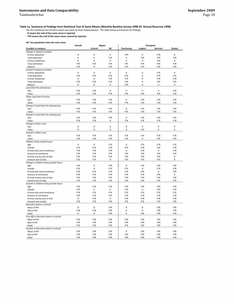
Table 1a. Summary of Findings from Statistical Test of Same Means (Monthly Baseline Survey 1998 VS. Annual Resurvey 1998)The first statistical test of same means was done by Anan Pawasutipaisit. The table below summarizes his findings.
R means the null of the same mean is rejected
FTR means the null of the same mean cannot be rejected
H0: Two populations have the same mean
Overall
Variable to compare Central NE Chachoeng Lopburi Buriram Sisaket
First Difference of Income
Total income FTR FTR FTR FTR FTR FTR FTR
Per capita FTR FTR FTR FTR FTR FTR FTR
Weighted per capita FTR FTR FTR FTR FTR FTR FTR
Growth of Income
Total income FTR FTR FTR FTR FTR FTR FTR
Per capita FTR FTR FTR FTR FTR FTR FTR
Weighted per capita FTR FTR FTR FTR FTR FTR FTR
First Difference of Consumption
Total Consumption FTR FTR FTR FTR FTR FTR FTR
Per capita FTR FTR FTR FTR FTR FTR R
Weighted per capita FTR FTR FTR FTR FTR FTR FTR
Growth of Consumption
Total Consumption FTR FTR FTR FTR FTR FTR FTR
Per capita FTR FTR FTR FTR FTR FTR FTR
Weighted per capita FTR FTR FTR FTR FTR FTR FTR
Occupation
Agriculture R R R R R R R
Business R R R R R R R
Wage R R R R R R R
Change in occupation
Agriculture R R R R R R R
Business R R R R R R R
Wage R R R R R R R
Household size FTR FTR FTR FTR R R R
Change in HH size FTR FTR FTR FTR R FTR FTR
Borrowing variables
Borrow R R FTR R R FTR FTR
Payback R R R R FTR R FTR
Annual reported interest rate R FTR R FTR FTR R R
How long FTR R FTR FTR R R FTR
Annual calculated interest rate FTR FTR R FTR R R FTR
Change in Borrowing variables
Borrow FTR FTR FTR FTR FTR FTR FTR
Payback FTR R FTR FTR FTR FTR FTR
How long FTR FTR FTR R FTR FTR FTR
Annual calculated interest rate FTR FTR FTR FTR FTR FTR FTR
Annual reported interest rate FTR FTR R FTR FTR FTR R
G th i B i i bl
ChangwatRegion
Growth in Borrowing variables
Borrow FTR FTR FTR FTR FTR FTR FTR
Payback FTR FTR FTR FTR FTR FTR FTR
Length of loan FTR FTR FTR R FTR FTR FTR
Annual calculated interest rate FTR FTR FTR R FTR FTR FTR
Annual reported interest rate FTR FTR R R FTR FTR R
Lending variables
Lend FTR FTR FTR FTR FTR FTR FTR
Payback FTR FTR FTR FTR FTR FTR FTR
Annual reported interest rate FTR R FTR R FTR FTR FTR
How long FTR FTR FTR FTR FTR R FTR
Annual calculated interest rate FTR FTR FTR FTR FTR FTR R
Change in Lending variables
Lend FTR FTR FTR FTR FTR FTR FTR
Payback FTR FTR FTR FTR FTR FTR FTR
How long R FTR FTR FTR FTR FTR FTR
Annual calculated interest rate R FTR R FTR FTR FTR FTR
Annual reported interest rate FTR FTR FTR FTR FTR FTR FTR
Growth in Lending variables
Lend FTR FTR FTR FTR FTR FTR FTR
Payback FTR FTR FTR FTR FTR R FTR
How long FTR FTR R FTR FTR FTR FTR
Annual calculated interest rate FTR FTR R FTR FTR FTR FTR
Annual reported interest rate FTR FTR FTR FTR FTR FTR FTR
Deposit variables
# times deposited R R R R R R R
Total deposited R R FTR R R FTR FTR
# times withdrawn R R R R R FTR R
Total withdrawn R R FTR R R FTR FTR
Balance R R R R FTR R R
Instruments and Data ComparabilityTambunlertchai
September 2009Page 10
Table 1a. Summary of Findings from Statistical Test of Same Means (Monthly Baseline Survey 1998 VS. Annual Resurvey 1998)The first statistical test of same means was done by Anan Pawasutipaisit. The table below summarizes his findings.
R means the null of the same mean is rejected
FTR means the null of the same mean cannot be rejected
H0: Two populations have the same mean
Overall
Variable to compare Central NE Chachoeng Lopburi Buriram Sisaket
ChangwatRegion
Change in Deposit variables
# times deposited R R R FTR R FTR R
Total deposited R R FTR R FTR FTR FTR
# times withdrawn R R R R R FTR R
Total withdrawn FTR FTR FTR FTR FTR FTR FTR
Balance FTR R FTR FTR FTR FTR FTR
Growth in Deposit variables
# times deposited R R R R R FTR R
Total deposited FTR FTR FTR FTR R FTR FTR
# times withdrawn R R FTR FTR R FTR FTR
Total withdrawn FTR FTR FTR FTR R FTR FTR
Balance R R R FTR R R R
Land that HH cultivate/use
Size FTR FTR R R R R FTR
Value FTR FTR FTR FTR FTR FTR FTR
Other Land that HH owns
Size FTR FTR FTR R FTR FTR FTR
Value FTR FTR FTR FTR FTR FTR FTR
Change in Land that HH cultivate/use
Size FTR FTR FTR R FTR FTR FTR
Value FTR FTR FTR FTR FTR FTR FTR
Growth in Land that HH cultivate/use
Size FTR FTR FTR R FTR FTR FTR
Value FTR FTR R FTR FTR FTR FTR
Change in Other Land
Size R R R R R R R
Value R R R R FTR R R
Growth in Other Land
Size FTR FTR FTR FTR FTR FTR FTR
Value FTR FTR FTR FTR R FTR FTR
Children living outside house
Age R R FTR R FTR FTR FTR
Gender FTR FTR FTR FTR FTR FTR FTR
# times kids send remittance FTR FTR FTR R FTR R FTR
Amount of remittance FTR FTR FTR FTR FTR FTR FTR
# times money sent to kids FTR FTR FTR FTR FTR FTR R
Amount sent to kids FTR FTR R FTR FTR FTR R
Change in Children living outside house
Age FTR R FTR R FTR FTR FTR
Gender FTR R FTR FTR R FTR FTR
# times kids send remittance FTR FTR FTR FTR FTR R FTR
Amount of remittance FTR FTR FTR FTR FTR FTR R
# times money sent to kids FTR FTR FTR FTR FTR FTR FTR
Amount sent to kids FTR FTR FTR FTR FTR FTR FTR
Growth in Children living outside house
Age FTR FTR FTR FTR FTR FTR FTR
Gender FTR R R FTR R FTR FTR
# times kids send remittance FTR FTR FTR FTR FTR FTR FTR
Amount of remittance FTR FTR FTR FTR FTR FTR FTR
# times money sent to kids R FTR R FTR FTR FTR FTR
Amount sent to kids FTR FTR FTR FTR FTR FTR FTR
Education (years in school)
Mean of HH R R FTR R R FTR FTR
Max of HH FTR FTR FTR R R FTR FTR
Head R R FTR R FTR FTR FTR
First diff in Education (years in school)
Mean of HH FTR FTR FTR FTR FTR FTR FTR
Max of HH FTR FTR FTR FTR FTR FTR FTR
Head FTR FTR FTR FTR FTR FTR FTR
Growth in Education (years in school)
Mean of HH FTR FTR FTR R FTR FTR FTR
Max of HH FTR FTR FTR FTR FTR FTR FTR
Head FTR FTR FTR FTR FTR FTR FTR

Instruments and Data ComparabilityTambunlertchai
September 2009Page 11
The results show that for most of the variables, we fail to reject the null that the two samples have thesame means. These variables include income, consumption, education, demographics of children livingoutside the households, some land variables, and most of the growth variables in income, consumption,lending, and borowing. The two samples, however, seem to differ in terms of occupations both atthe overall and at the regional levels. Proportions of households engaged in agrigulture and business,as well as those that work as wage earners are statistically different across the two datasets. Thedifferent occupational components of the two datasets may explain some of the other differences atemerge in other variables.
At the provincial level, we see differences in deposit, lending, and borrowing variables. The two Buriramsubsamples, for example, differ in terms of loan payback rates, loan interest rates, and loan terms.Borrowing rates and loan terms are also different for the Lopburi subsamples. The Chachoengsao andLopburi subsamples have different deposit and withdrawal frequencies as well as different total values ofdeposits or withdrawals. Changes in these variables across the two datasets, however, do not seem todiffer much, implying that the differences are not driven by divergent growth rates. These differencesin bank transaction variables may indicate that households in the two samples have dissimilar accessto financial institutions, although no further work has been done to allow for this conclusion.
The second set of mean comparisons test pairs the each year of the Annual Resurvey data with thecorresponding annualized Monthly data from 2000 to 2005. Unlike the annualization done before,Monthly data were annualized in such a way that made each "year" directly comparable to its Annualcounterpart. To illustrate this point, consider for example the 2000 Annual Resurvey data. Theseare recall information that pertain to the period from May 1999 to April 2000. To construct the 2000annualized Monthly data for the mean comparison test, therefore, the same time period is used. Thismethod of aggregation is the reason why there is no annualized Monthly data for 1999. The Monthlydata, which start only in September 1998, do not go back far enough to permit 1999 annualization.
Unlike the Big Survey questionnaire and the Monthly Baseline Survey questionnaire which were similarto each other, the questionnaires for the Annual Resurvey and the Monthly Survey differ considerablyfrom each other. The second round of tests was performed on a more limited set of variables. Theresults from these t-tests are presented in Table 1b.

Instruments and Data ComparabilityTambunlertchai
September 2009Page 12
Table 1b. Summary of Findings from Statistical Test of Same Means (Monthly Survey VS. Annual Resurvey from 1999 ‐ 2005)R means the null of the same mean is rejected at the 0.1 confidence levelFTR means the null of the same mean cannot be rejected
H0: Two populations have the same mean
Monthly data were annualized such that they matched up with Annual resurvey timeframe
Overall
2000 2001 2002 2003 2004 2005
Revenue
Cultivation revenue FTR FTR FTR FTR FTR R
Livestock revenue R R R R R R
Fish/Shrimp revenue R R R R R R
Business revenue FTR FTR FTR FTR FTR FTR
Wage revenue R R R R R R
Interest revenue R R R R R R
Net income FTR FTR FTR R FTR FTR
Expense
Farm expense R R FTR FTR R FTR
Shrimp/Fish expense R R R R R R
Business expense R R R FTR FTR FTR
Regional
Central NE Central NE Central NE Central NE Central NE Central NE
Revenue
Cultivation revenue R R FTR R FTR R FTR R R R R FTR
Livestock revenue R R R R R R R R R R R R
Fish/Shrimp revenue R R R R R R R R R R R R
Business revenue FTR FTR FTR FTR FTR FTR FTR FTR FTR FTR FTR FTR
Wage revenue FTR FTR FTR R FTR R FTR R FTR R FTR R
Interest revenue R R R R R R R R R R R R
Net income R R R R FTR R FTR R FTR FTR FTR R
20052000 2001 2002 2003 2004
Net income R R R R FTR R FTR R FTR FTR FTR R
Expense R R R R R R R R R R R R
Farm expense R FTR R R FTR R R R R R FTR R
Shrimp/Fish expense R FTR R FTR R FTR R R R FTR R FTR
Business expense FTR FTR FTR FTR FTR FTR R FTR FTR FTR R FTR
Total Consumption R R R R R FTR R FTR R FTR R FTR

Instruments and Data ComparabilityTambunlertchai
September 2009Page 13
This second round of tests rejects the null of same sample means at a higher frequency than in the firstround. The higher rejection rate could be due to the annualization of monthly variables, althoughwe were careful to standardize the timeframes being compared. It could also be the case that thetwo subsamples diverge over time as an accumulated result of local economic conditions. This seemsunlikely, however, as it is not obvious that the null rejection rate is growing over time.
These findings do not provide a clear answer on whether the two datasets are comparable. A bigconcern that emerges is that the way in which the underlying variables are constructed may have ledto the evidently different trends in the two samples. To see why this may be a concern, consider,for example, livestock revenue data. This information on the Annual Resurvey is based on figuresprovided by the households. In the Monthly Survey, households are asked detailed questions aboutlivestock activities, and livestock revenue is backed out from this information. If the method of backingout this variable is incorrect, there will be no useful links between the two datasets.
To investigate whether this were indeed the case, we next narrow our focus on those households thatwere exposed to both the Annual and the Monthly questionnaires.
Analysis of Overlap
To see if different construction of variables (that are intended to be the same) has led to the observeddifferences in the two datasets, we go back to the overlap of the Big Survey sample and the Monthlysample. Recall that the Monthly survey sample comprises a subset of the original Big Survey as wellas additional households.
2Overlap
1.jpg
This overlap is valuable for this next exercise because households in here are those that were initiallyinterviewed in May 1997, then re-sampled and interviewed in the 1998 Monthly Baseline Survey, andsubsequently remained in the Monthly Surveys. In other words, these are the households that werefirst interviewed with annual-type instruments (Big Survey of 1997 and Baseline Survey of 1998),

Instruments and Data ComparabilityTambunlertchai
September 2009Page 14
and then with monthly-type instruments (Monthly Survey beginning in 1999). Since the underlyingpopulation did not change, one would expect the time series of household variables to be relativelysmooth over time. If the two types of questionnaires extracted the same information, and the twosets of variables were constructed in such a way that made them comparable, we would not expect tosee any disruptions in the time series between 1998 and 1999, the point of transition between the twotypes of questionnaires.
Focusing on this subsample reduces the sample size for analysis to around 55-60 households per provinceper year. Four forms of averages were calculated—using all data, dropping zeros, dropping outliers,and dropping both zeros and outliers, where outliers are defined as values that lie above or below2.5 standard deviations from the mean. Dropping outliers from the samples got rid of some distur-bances, while dropping zeros merely shifted the graphs upward slightly. Figure 3 shows the graphicalsummaries of the time series. Here only the averages without outliers are presented.

Instruments and Data ComparabilityTambunlertchai
September 2009Page 15
Figure 3a. Time Series Average (2005 Thai Baht): CHACHOENGSAO1997 Annual Survey (Big Survey) and Monthly Survey Overlap
0
10000
20000
30000
40000
50000
60000
70000
80000
90000
100000
1997 1998 1999 2000 2001 2002 2003 2004 2005
Chachoengsao: Revenue by Source (excl. outliers) (2005 Thai Bt)Subsample of households that are in both 1997 Big Survey and Monthly Survey
Cultivation
Livestock
Wage
Shrimp/Fish
Business
40000
60000
80000
100000
120000
140000
Chachoengsao: Expense by Source (excl outliers) (2005 Thai Bt)Subsample of households that are in both 1997 Big Survey and Monthly Survey
Cultivation
Livestock
Wage
Shrimp/Fish
0
10000
20000
30000
40000
50000
60000
70000
80000
90000
100000
1997 1998 1999 2000 2001 2002 2003 2004 2005
Chachoengsao: Revenue by Source (excl. outliers) (2005 Thai Bt)Subsample of households that are in both 1997 Big Survey and Monthly Survey
Cultivation
Livestock
Wage
Shrimp/Fish
Business
0
20000
40000
60000
80000
100000
120000
140000
1997 1998 1999 2000 2001 2002 2003 2004 2005
Chachoengsao: Expense by Source (excl outliers) (2005 Thai Bt)Subsample of households that are in both 1997 Big Survey and Monthly Survey
Cultivation
Livestock
Wage
Shrimp/Fish
Business
0
100000
200000
300000
400000
500000
600000
700000
800000
1997 1998 1999 2000 2001 2002 2003 2004 2005
Chachoengsao: Gross Rev, Gross Exp, Net Inc (excl outliers) (2005 Thai Bt)Subsample of households that are in both 1997 Big Survey and Monthly Survey
Gross revenue
Gross expense
Net income

Instruments and Data ComparabilityTambunlertchai
September 2009Page 16
Figure 3b. Time Series Average (2005 Thai Baht): LOPBURI1997 Annual Survey (Big Survey) and Monthly Survey Overlap
0
20000
40000
60000
80000
100000
120000
140000
160000
1997 1998 1999 2000 2001 2002 2003 2004 2005
Lopburi: Revenue by Source (excl outliers) (2005 Thai Baht)Subsample of households that are in both 1997 Big Survey and Monthly Survey
Cultivation
Livestock
Wage
Shrimp/Fish
Business
30000
40000
50000
60000
70000
80000
90000
100000
Lopburi: Expense by Source (excl outliers) (2005 Thai Baht)Subsample of households that are in both 1997 Big Survey and Monthly Survey
Cultivation
Livestock
Wage
Shrimp/Fish
0
20000
40000
60000
80000
100000
120000
140000
160000
1997 1998 1999 2000 2001 2002 2003 2004 2005
Lopburi: Revenue by Source (excl outliers) (2005 Thai Baht)Subsample of households that are in both 1997 Big Survey and Monthly Survey
Cultivation
Livestock
Wage
Shrimp/Fish
Business
0
10000
20000
30000
40000
50000
60000
70000
80000
90000
100000
1997 1998 1999 2000 2001 2002 2003 2004 2005
Lopburi: Expense by Source (excl outliers) (2005 Thai Baht)Subsample of households that are in both 1997 Big Survey and Monthly Survey
Cultivation
Livestock
Wage
Shrimp/Fish
Business
0
50000
100000
150000
200000
250000
300000
350000
400000
450000
1997 1998 1999 2000 2001 2002 2003 2004 2005
Lopburi: Gross Rev, Gross Exp, Net Inc (excl outliers) (2005 Thai Bt)Subsample of households that are in both 1997 Big Survey and Monthly Survey
Gross revenue
Gross expense
Net income

Instruments and Data ComparabilityTambunlertchai
September 2009Page 17
Figure 3c. Time Series Average (2005 Thai Baht): BURIRAM1997 Annual Survey (Big Survey) and Monthly Survey Overlap
0
5000
10000
15000
20000
25000
30000
35000
40000
45000
50000
1997 1998 1999 2000 2001 2002 2003 2004 2005
Buriram: Revenue by Source (excl outliers) (2005 Thai Baht)Subsample of households that are in both 1997 Big Survey and Monthly Survey
Cultivation
Livestock
Wage
Shrimp/Fish
Business
60000
80000
100000
120000
140000
160000
180000
200000
Buriram: Expense by Source (excl outliers) (2005 Thai Baht)Subsample of households that are in both 1997 Big Survey and Monthly Survey
Cultivation
Livestock
Wage
Shrimp/Fish
0
5000
10000
15000
20000
25000
30000
35000
40000
45000
50000
1997 1998 1999 2000 2001 2002 2003 2004 2005
Buriram: Revenue by Source (excl outliers) (2005 Thai Baht)Subsample of households that are in both 1997 Big Survey and Monthly Survey
Cultivation
Livestock
Wage
Shrimp/Fish
Business
0
20000
40000
60000
80000
100000
120000
140000
160000
180000
200000
1997 1998 1999 2000 2001 2002 2003 2004 2005
Buriram: Expense by Source (excl outliers) (2005 Thai Baht)Subsample of households that are in both 1997 Big Survey and Monthly Survey
Cultivation
Livestock
Wage
Shrimp/Fish
Business
‐50000
0
50000
100000
150000
200000
250000
300000
1997 1998 1999 2000 2001 2002 2003 2004 2005
Buriram: Gross Rev, Gross Exp, Net Inc (excl outliers) (2005 Thai Bt)Subsample of households that are in both 1997 Big Survey and Monthly Survey
Gross revenue
Gross expense
Net income

Instruments and Data ComparabilityTambunlertchai
September 2009Page 18
Figure 3d. Time Series Average (2005 Thai Baht): SISAKET1997 Annual Survey (Big Survey) and Monthly Survey Overlap
0
5000
10000
15000
20000
25000
30000
35000
40000
45000
1997 1998 1999 2000 2001 2002 2003 2004 2005
Sisaket: Revenue by Source (excl outliers) (2005 Thai Baht)Subsample of households that are in both 1997 Big Survey and Monthly Survey
Cultivation
Livestock
Wage
Shrimp/Fish
Business
10000
15000
20000
25000
30000
Sisaket: Expense by Source (excl outliers) (2005 Thai Baht)Subsample of households that are in both 1997 Big Survey and Monthly Survey
Cultivation
Livestock
Wage
Shrimp/Fish
0
5000
10000
15000
20000
25000
30000
35000
40000
45000
1997 1998 1999 2000 2001 2002 2003 2004 2005
Sisaket: Revenue by Source (excl outliers) (2005 Thai Baht)Subsample of households that are in both 1997 Big Survey and Monthly Survey
Cultivation
Livestock
Wage
Shrimp/Fish
Business
0
5000
10000
15000
20000
25000
30000
1997 1998 1999 2000 2001 2002 2003 2004 2005
Sisaket: Expense by Source (excl outliers) (2005 Thai Baht)Subsample of households that are in both 1997 Big Survey and Monthly Survey
Cultivation
Livestock
Wage
Shrimp/Fish
Business
0
20000
40000
60000
80000
100000
120000
140000
1997 1998 1999 2000 2001 2002 2003 2004 2005
Sisaket: Gross Rev, Gross Exp, Net Inc (excl outliers) (2005 Thai Bt)Subsample of households that are in both 1997 Big Survey and Monthly Survey
Gross revenue
Gross expense
Net income

Instruments and Data ComparabilityTambunlertchai
September 2009Page 19
The graphical summaries show notably smooth trends at the point of transition, between 1998 and1999. This gives us some comfort on two levels. First, the same variables constructed separately seemcomparable across instruments. Second, changing from the Annual to the Monthly questionnaire didnot result in any apparent disruption in time trends. The different trends across the two samplesthat prompted this study therefore are unlikely to be driven by faulty variable construction or ques-tionnaire differences. While it should be noted that some extreme swings are seen in Chachoengsao’srevenue variables and Sisaket’s expense variables between 1997 and 1999. But these swings do notsystematically appear across all variables, and are likely attributable to repercussions from the 1997financial crisis.
Household Accounting
One problem that has become apparent in the process comparing the Annual and Monthly data is thediffi culty in directly comparing the two datasets. The different time intervals of the surveys turn out toonly be a minor hindrance for the Monthly data can be easily aggregated up to the annual level. Thebigger obstacles are the considerably different variables in the two datasets. For example, consumptionin the Annual data is defined differently from that in the Monthly data, or farm income in the Annualdata is inclusive of all agricultural activities, whereas the Monthly data break agricultural income intocultivation, livestock, livestock depreciation and livestock capital losses. This has meant that muchtime was spent manipulating variables so that they could be compared, in the end yielding only a fewvariables that were used for the comparison. A standardization of how household activities translateinto income, costs, and profits is needed to bridge the two datasets. The accounting method providesa natural template for doing this. Mapping household and entrepreneurial activities from each datasetto financial account activities can help standardize the variables, simplifying the comparison of thetwo databases as well as their uses going forward.
The idea behind this comes from Samphantharak and Townsend (2009) 1 , who treat households ascorporate firms and apply the corporate accounting framework to create household financial statementsfrom the Monthly data. Their work systematically maps Monthly household variables into balancesheet and income statement items, which has greatly simplified and enhanced the use of the Monthlydata. Moreover, with the balance sheet and the income statement, household cash balances, which arenot directly asked for in the questionnaires, can be backed out via the statement of cash flow methods.
With the Monthly financial statements on hand, the next step is to construct their annual analoguesfrom the Annual Resurvey data. Initial work has shown that the coarser information available in theAnnual data will not permit a construction of identical financial statements, and many challenges havesurfaced which we discuss below.
Initial Challenges
The accounting methodology forces a more detailed look at the variables in the Annual data and howconsumption, saving, and investment activities translate into their stock and flow over time. Thiscloser examination has brought out some inconsistencies in certain variables that will need to beaddressed prior to pushing ahead with the financial statements. This section summarizes the mainobstacles that have come up in the process.
One of the first challenges is figuring out investment flows from the asset module in the Annualquestionnaire. This module comprises three submodules for agricultural, household, and business
1Samphantharak, Krislert and Robert M. Townsend, (2009), "Households as Corporate Firms: An Analysis ofHousehold Finance Using Integrated Household Surveys and Corporate Financial Accounting," Cambridge UniversityPress.

Instruments and Data ComparabilityTambunlertchai
September 2009Page 20
assets. The agricultural and household asset submodules each gives respondents a list of specificassets and asks whether or not the households have them, and if they do, how much they are worth,how long they have had them, and how their acquisitions were financed. Finally respondents are alsoasked whether their households got rid of any assets in the past year and how they were disposedof (sold for cash, thrown away, gifted away, etc.). All this information can be used to compute thevalue of agricultural and household assets at a given point in time, the changes due to investment anddivestment, as well as the cash flow associated with the transactions. Assets that are broken, lost, orthrown away are recorded as capital loss. With renovations, we record the values of the assets priorto renovation as capital loss because the values of the renovations are recorded as new investments.The agricultural and the household asset submodules, therefore, provide enough information for thefinancial statements.
A problem arises with when we move to the business asset submodule. Rather than giving respondentsa list of assets as before, this submodule asks households to list their own business assets, how muchthey are worth, and how long the household has had them. Because the term "business" encompassesmany different types of entrepreneurial activities, offering respondents the flexibility of listing theirown assets has the obvious benefit of not missing out on unanticipated assets. The price of thisflexibility is the inconsistency in reporting across households as well as within households over time.These inconsistencies will require a considerable amount of time to correct for.
Because there is no standardization for what goes into the business asset submodule, some householdsover-report what they consider to be business assets while others under-report. One of the moresubstantive consequences of this is that some households report inventory as business assets whileothers do not. Some households also report structures such as "house" or "1/4 of house", or "building"or "ponds" as business assets. In constructing the financial statements from the Annual data, reportedinventory may have to be left out from asset calculations. Since there is no separate module for itin the Annual questionnaire, including inventory as business assets would underestimate the assetsof households that fail to report it. Buildings and other structures attached to the land reportedas business assets should also be re-categorized as "land improvement" in the household financialstatement.
Incidence of double counting is also non trivial. Many households, for example, report livestockas their business assets. The problem is that there is a separate module for livestock where suchassets should have already been reported. Mills, tractors, rice thrashing machines, etc., which shouldhave already been reported in the agricultural asset submodule also frequently appear in the businessasset submodule. Household assets such as motorcycles and cars also get reported as business assets.Lastly, many households also include land, which belong to the land module, as their business assets.To a large extent, such overlaps in asset reporting are likely due blurred lines between household andbusiness assets in informal businesses which usually operate out of the home. Our concern is that theseoverlaps are causing double-counts of assets, and would lead to non-negligible measurement errors asmany of these items are of significant values.
Correcting for potential double counts requires manually going through the asset entries to remove themiscategorized assets. We then cross check whether these miscategorized assets have been reportedin their appropriate module— if so, the double counts are deleted, otherwise, they get attributed totheir proper accounts. Of course recategorizing an entry in a given year requires that we look for thatasset in the subsequent years and also duely recategorize it. This correction process has taken a lotof time not only because of the large amount of data in the panel, but also because of the spellinginconsistencies in the data. The same asset may be reported under different names across time asenumerators change, making it diffi cult to track a certain asset over time. Variations in spellingsexarcerbate the problem. The inconsistency in asset names creates a further problem when we wantto merge asset data across time to form an amortization schedule. For example, the "barber chair"

Instruments and Data ComparabilityTambunlertchai
September 2009Page 21
reported in 1998 might become "barber bench" in 1999 or "haircut bench" in 2000. Similarly, "50chickens" which need to be taken out from business asset because they should be in the livestockmodule can change in the next year to "40 chicks" or "45 hens," etc. So after the data are cleaned ofdouble-counts, we will have to manually match assets across time in order to amortize them.
While these corrections are time-consuming and quite tedious, they are not especially diffi cult to do.Once they are done, we can be more comfortable with our estimates of assetholding in a given year.However, a rather important problem remains. The biggest problem in the business asset submodulelies in the fact that there is no question that asks about how the assets are financed, and nothingabout whether households got rid of any business assets in the past year. This turns out to be amajor hindrance for constructing the financial statements. When a new asset shows up in the data,one cannot know how much to attribute its acquisition to credit, how much to cash, and how muchto contributed capital. When previously reported assets disappear in the next year, it is diffi cultto determine whether they were gifted away, retired from use, or sold. The lack of information herewill affect our estimates of cash, credit financing, and capital losses. This means that even when theaforementioned inconsistencies have been addressed, these errors will remain.
While the potentially lengthy correction process is underway, the data at hand remain the most detailedrecords available of household transactions. Much information can be gleaned from these data whilekeeping in mind the potential measurement errors. One variable of particular interest is households’cash holdings. Since households are not directly asked about the amounts of cash they have onhand, the Annual and the Monthly data can provide a rough estimate of these amounts. Withoutcorrecting for the aforementioned errors, cash estimates can be obtained rather quickly. The nextsection discusses the estimate of cash from the Annual data, and how these estimates compare to theavailable estimates obtained from the Monthly instrument. As we will see, the two sets of estimatesdo not quite line up.
Cash Estimates
Ignoring the errors in asset investment discussed above for now, the following equation expresses thedeficit in household spending that must be financed with cash:
−∆Casht = Ct + It −NetIncomet −Borrowingst − SavingsWithdrawnt (1)
where Ct is weighted consumption, It is investment in asset and land.
The weighted consumption makes use of changwat-specific weights from Jeong (2008). Net incomeis household gross income net of operating (farm and business) expenses. Investments It are thenet cash-financed investments in household assets, agricultural assets, business assets, as well as land.Cash-financed purchases of equipment and land are cash outflows while sales for cash are inflows. Notethat, as discussed above, investments in business asset are subject to considerable measurement errordue to the potential double-count issues as well as the fact that this submodule does not record assetdisposals. Since we are not correcting for these issues at this time, the investment variable is quitenoisy. Double counting cash-financed investments will depress estimates of cash balances since wemay be overstating cash outflows. Not accounting for asset disposal will also bias downward cashestimates since we are not accounting for inflows from cash sales of assets. It should be re-emphasizedtherefore that results from this section are purely meant to provide a rough first guess at the level ofcash holdings in the Annual data.
Borrowingst are those new borrowings (cash inflow) made in that year. We consider borrowings

Instruments and Data ComparabilityTambunlertchai
September 2009Page 22
net of any lending that households may have made in the year since the latter are cash outflows.The variable SavingsWithdrawnt considers savings withdrawn in year t net of deposits made by thehouseholds in that year.
To get estimates of cash holdings, we make the assumption that households’initial cash balances attime 0, Cash0, are zero. Equation (1) gives us the annual change in cash which would get added tothe beginning balance. The beginning balance at time t is the amount of cash the household has atthe beginning of period t The ending balance is the beginning balance plus the change in cash in thatyear. This is used used as the following year’s beginning balance. Formally,
BB0 = 0
EBt = BBt + ∆Casht for t ≥ 0
BBt+1 = EBt
where BBt and EBt are beginning and ending balances in year t, respectively. Since cash balancemust always be non-negative, each time the change in cash is added to the existing balance, we checkthat the change does not cause EB to fall below zero. If cash balance becomes negative, Cash0 isadjusted upward by the absolute value of that negative amount. For example, if cash balance becomes−τ in a certain year, Cash0 is adjusted up by τ since the household must have begun with at least thatmuch in order for their cash balance to stay non-negative. The cash balance estimation in the Monthlydata uses this same methodology, where initial cash holding is assumed to be zero until adjustmentsare needed.
This method of estimating cash has the shortcoming in that it may underestimate initial cash holdingssince it assumes zero intial balances. In particular, it underestimates the initial cash holdings ofhouseholds that have high operating profits, borrowings, or saving withdrawals. This is because thesehouseholds are less likely to see negative cash balances which would require adjusting their initialbalances upward.
Results of the estimation are shown in Figures 4a and 4b. Because the Annual survey is fielded inMay of each year, we use the May cash balance from the Monthly data for comparisons. Note thatthe Monthly cash estimation begins in 1998. When estimating cash holding from the Annual data,we tried using both 1997 and 1998 as the initial period t = 0 but found little difference. The profile ofcash estimates starting in 1998 is basically a parallel shift downward by what would have been the cashholding in 1997 had it been included. Because of these similarities, we report in Figures 4a and 4bonly the estimates using 1997 as the starting point. These figures reveal that Annual cash estimatesfar exceed those of the Monthly. In a way, this is not surprising because in our methodology, cash isestimated as the residual amount needed to fulfill Equation (1). Unlike the Monthly survey which isfielded at a higher frequency and has the more detailed questions, the Annual survey likely misses quitea few transactions because of the longer recall period and the less detailed nature of the questionnaire.So data issues aside, it is likely that many transactions are left out of the high-frequency transactionitems like Ct and It, causing the residual ∆Casht to be quite large and thereby pushing upward ourestimate of cash in the Annual data.

Instruments and Data Comparability
Tambunlertchai
September 2009
Page 23
Figure 4a. Comparison of Cash Balance EstimatesNortheast and Central data
1,000,000
1,200,000
End‐of‐Year Cash Balance (Northeast)
400,000
600,000
800,000
1,000,000
1,200,000
Thai Bah
t
End‐of‐Year Cash Balance (Northeast)
‐
200,000
400,000
600,000
800,000
1,000,000
1,200,000
1997 1998 1999 2000 2001 2002 2003 2004 2005 2006
Thai Bah
t
End‐of‐Year Cash Balance (Northeast)
Northeast avg (Annual data) Northeast avg (Monthly data)
‐
200,000
400,000
600,000
800,000
1,000,000
1,200,000
1997 1998 1999 2000 2001 2002 2003 2004 2005 2006
Thai Bah
t
End‐of‐Year Cash Balance (Northeast)
Northeast avg (Annual data) Northeast avg (Monthly data)
2,000,000
2,500,000
End‐of‐Year Cash Balance (Central)
‐
200,000
400,000
600,000
800,000
1,000,000
1,200,000
1997 1998 1999 2000 2001 2002 2003 2004 2005 2006
Thai Bah
t
End‐of‐Year Cash Balance (Northeast)
Northeast avg (Annual data) Northeast avg (Monthly data)
500 000
1,000,000
1,500,000
2,000,000
2,500,000
Thai Bah
t
End‐of‐Year Cash Balance (Central)
‐
200,000
400,000
600,000
800,000
1,000,000
1,200,000
1997 1998 1999 2000 2001 2002 2003 2004 2005 2006
Thai Bah
t
End‐of‐Year Cash Balance (Northeast)
Northeast avg (Annual data) Northeast avg (Monthly data)
‐
500,000
1,000,000
1,500,000
2,000,000
2,500,000
1997 1998 1999 2000 2001 2002 2003 2004 2005 2006
Thai Bah
t
End‐of‐Year Cash Balance (Central)
Central avg (Annual data) Central avg (Monthly data)

Instruments and Data Comparability
Tambunlertchai
September 2009
Page 24
Figure 4b. Comparison of Cash Balance EstimatesChangwat‐level data
1,200,000
1,400,000
1,600,000
End‐of‐Year Cash Balance (Buriram)
1,000,000
1,200,000
1,400,000
End‐of‐Year Cash Balance (Sisaket)
‐
200,000
400,000
600,000
800,000
1,000,000
1,200,000
1,400,000
1,600,000
1997 1998 1999 2000 2001 2002 2003 2004 2005 2006
End‐of‐Year Cash Balance (Buriram)
‐
200,000
400,000
600,000
800,000
1,000,000
1,200,000
1,400,000
1997 1998 1999 2000 2001 2002 2003 2004 2005 2006
End‐of‐Year Cash Balance (Sisaket)
‐
200,000
400,000
600,000
800,000
1,000,000
1,200,000
1,400,000
1,600,000
1997 1998 1999 2000 2001 2002 2003 2004 2005 2006
End‐of‐Year Cash Balance (Buriram)
Buriram (Annual data)
Buriram (Monthly data)
‐
200,000
400,000
600,000
800,000
1,000,000
1,200,000
1,400,000
1997 1998 1999 2000 2001 2002 2003 2004 2005 2006
End‐of‐Year Cash Balance (Sisaket)
Sisaket (Annual data)
Sisaket (Monthly data)
E d f Y C h B l (Ch h ) E d f Y C h B l (L b i)
‐
200,000
400,000
600,000
800,000
1,000,000
1,200,000
1,400,000
1,600,000
1997 1998 1999 2000 2001 2002 2003 2004 2005 2006
End‐of‐Year Cash Balance (Buriram)
Buriram (Annual data)
Buriram (Monthly data)
‐
200,000
400,000
600,000
800,000
1,000,000
1,200,000
1,400,000
1997 1998 1999 2000 2001 2002 2003 2004 2005 2006
End‐of‐Year Cash Balance (Sisaket)
Sisaket (Annual data)
Sisaket (Monthly data)
500,000
1,000,000
1,500,000
2,000,000
2,500,000
End‐of‐Year Cash Balance (Chachoengsao)
500 000
1,000,000
1,500,000
2,000,000
2,500,000
End‐of‐Year Cash Balance (Lopburi)
‐
200,000
400,000
600,000
800,000
1,000,000
1,200,000
1,400,000
1,600,000
1997 1998 1999 2000 2001 2002 2003 2004 2005 2006
End‐of‐Year Cash Balance (Buriram)
Buriram (Annual data)
Buriram (Monthly data)
‐
200,000
400,000
600,000
800,000
1,000,000
1,200,000
1,400,000
1997 1998 1999 2000 2001 2002 2003 2004 2005 2006
End‐of‐Year Cash Balance (Sisaket)
Sisaket (Annual data)
Sisaket (Monthly data)
‐
500,000
1,000,000
1,500,000
2,000,000
2,500,000
1997 1998 1999 2000 2001 2002 2003 2004 2005 2006
End‐of‐Year Cash Balance (Chachoengsao)
Chachoengsao (Annual data)
Chachoengsao (Monthly data)
‐
500,000
1,000,000
1,500,000
2,000,000
2,500,000
1997 1998 1999 2000 2001 2002 2003 2004 2005 2006
End‐of‐Year Cash Balance (Lopburi)
Lopburi (Annual data)
Lopburi (Monthly data)

Instruments and Data ComparabilityTambunlertchai
September 2009Page 25
Conclusion and Next Steps
The Annual and Monthly data comparisons have given some insights into the nature of the two datasets.Based on the evidence thus far, it seems unlikely that the two underlying populations are equivalent.A close look at the datasets’comparability, however, has familiarized us with the scope of each dataset,and forced us to revisit the design of the questionnaires and the construction of the variables. Theevidence here reassures us of the validity of the the instruments and the variables that have been inuse.
Graphical summaries and mean comparison tests have shown that visually the Monthly and the Annualdata appear to be different but statistically we cannot conclusively reject that the two samples have thesame means. Since few variables from the two datasets can be directly compared, we are working onstandardizing the variables using methods in accounting to create balance sheets, income statements,and finally statements of cash flow. The last item will prove valuable because we do not directlyask for households’ cash holdings in the surveys. In implementing the standardization, we followSamphantharak and Townsend (2009) in the methods they use to create household financials from theMonthly data. We have since encountered a number of challenges and limitations in the datasets,particularly on the issues of double counting investments and underestimating asset disposals. Becausethe time intensity of the correction steps, this process has been somewhat prolonged.
While these issues are being addressed, we perform a rough estimate of the variable of interest—cash balances— ignoring potential measurement errors for the time being. This first pass at cashestimates show that estimates from the Annual data are significantly higher than those from theMonthly data. Not correcting for measurement errors in variables and the less detailed nature of theAnnual questionnaire likely contribute to the high estimate. The remaining part of the project willbe to finish the corrections of these variables and to come up with a way to extrapolate cashflows frombusiness asset investment and disposals since in this submodule, there is no information on financingmethods for acquisition or disposal methods for asset decreases.
Initial work has already shown that the coarser information in the Annual data will not permit aconstruction of financial statements that are identical to the Monthly statements. The standardizationprocess however will yield many Annual variables that can be used to compare and contrast withthe Monthly counterparts. Moreover, a careful revisit of the survey instruments will also help usdocument possible weaknesses in the current questionnaires as well as identify potential improvement.An updated Annual instrument may be a useful byproduct of the project..

APPENDIX
Table A. Bank of Thailand: Thailand's Macro Economic Indicatorshttp://www2.bot.or.th/statistics/ReportPage.aspx?reportID=409&language=engLast Updated : 30 Jan 2009 14:30Retrieved date : 24 Feb 2009 06:55
2008 p 2007 p 2006 2005 2004 2003 2002 2001 2000 1999 1998 1997
1 1. Population (Million persons) 63.04 63.04 62.83 62.42 61.97 63.08 62.80 62.31 61.88 61.80 61.20 60.502 2. GDP3 2.1 GDP at constant 1988 price (Billions of Baht) .... 4,259.6 4,059.6 3,858.0 3,688.1 3,468.1 3,237.0 3,073.6 3,008.4 2,871.9 2,749.6 3,072.64 (% change) .... 4.9 5.2 4.6 6.3 7.1 5.3 2.2 4.8 4.4 -10.5 -1.45 2.1.1 Agriculture (Billions of Baht) 1/ .... 370.5 364.0 347.8 354.4 363.0 322.1 320.0 309.9 289.1 282.6 286.86 (% change) .... 1.8 4.6 -1.8 -2.4 12.7 0.7 3.2 7.2 2.3 -1.5 -0.77 2.1.2 Non-agriculture (Billions of Baht) 1/ .... 3,889.0 3,695.6 3,510.1 3,333.7 3,105.1 2,914.8 2,753.5 2,698.4 2,582.8 2,467.0 2,785.78 (% change) .... 5.2 5.3 5.3 7.4 6.5 5.9 2.0 4.5 4.7 -11.4 -1.49 2.2 GDP at current price (Billions of Baht) .... 8,493.3 7,841.3 7,092.8 6,489.4 5,917.3 5,450.6 5,133.5 4,922.7 4,637.0 4,626.4 4,732.6
10 (% change) .... 8.3 10.6 9.3 9.7 8.6 6.2 4.3 6.2 0.2 -2.2 2.611 2.3 GNP per capita (Baht : Person) .... 123,673.4 114,748.0 103,667.8 96,049.2 88,688.0 82,975.2 79,571.6 77,860.1 72,980.6 72,979.2 76,057.412 3. Inflation13 3.1 Headline Consumer Price Index (2002=100) 123.4 117.0 114.4 109.3 104.6 101.8 100.0 99.4 97.8 96.2 96.0 88.814 (% change) 5.5 2.3 4.7 4.5 2.7 1.8 0.7 1.6 1.6 0.3 8.0 5.615 3.2 Core Consumer Price Index (2002=100) 2/ 108.1 105.6 104.5 102.2 100.6 100.2 100.0 99.6 98.4 97.6 95.9 89.516 (% change) 2.4 1.1 2.3 1.6 0.4 0.2 0.4 1.3 0.7 1.8 7.1 4.617 4. External Account18 4.1 Export (Billions of USD) 175.3 150.0 127.9 109.3 94.9 78.1 66.0 63.0 67.9 56.8 52.8 56.719 (% change) 16.8 17.2 16.9 15.1 21.5 18.1 4.7 -7.1 19.5 7.4 -6.7 3.820 4.2 Import (Billions of USD) 175.0 138.4 126.9 117.6 93.4 74.3 63.3 60.5 62.4 47.5 40.7 61.321 (% change) 26.4 9.0 7.9 25.8 25.7 17.3 4.5 -2.9 31.3 16.9 -33.7 -13.422 4.3 Trade balance (Billions of USD) 0.2 11.5 0.9 -8.2 1.4 3.7 2.7 2.4 5.5 9.3 12.2 -4.623 4.4 Current account balance (Billions of USD) -0.1 14.0 2.3 -7.6 2.7 4.7 4.6 5.1 9.3 12.5 14.3 -3.124 (as % of GDP) .... 5.7 1.1 -4.3 1.7 3.3 3.6 4.4 7.6 10.2 12.7 -2.025 4.5 Net capital movement (Billions of USD) 13.5 -2.4 6.8 11.0 3.6 -4.7 -1.8 -3.4 -10.3 -7.9 -9.8 -4.326 4.5.1 Private 3/ 14.7 1.6 7.2 9.5 3.2 -5.5 -3.3 -2.7 -9.8 -13.5 -15.4 -7.627 4.5.2 Public -1.2 -3.4 -0.9 1.3 -2.7 -1.9 -2.5 -0.3 -0.3 1.6 1.8 1.628 4.5.3 BOT 0.1 -0.6 0.4 0.2 3.0 2.6 4.0 -0.3 -0.2 4.0 3.9 1.729 4.6 Balance of payments (Billions of USD) 24.6 17.1 12.7 5.4 5.7 0.1 4.2 1.3 -1.6 4.6 1.7 -10.630 4.7 International reserves (Billions of USD) 111.0 87.4 67.0 52.1 49.8 42.1 38.9 33.0 32.7 34.8 29.5 27.031 4.8 Swap Obligation (Billions of USD) -6.9 -19.0 -6.9 -3.8 -4.6 -5.2 0.5 2.1 2.1 4.8 6.5 18.032 4.9 Total debt outstanding (Billions of USD) 64.3 61.7 59.6 52.0 51.3 51.8 59.5 67.5 79.7 95.0 105.0 109.233 of which : Public debt 4/ 12.2 12.0 13.1 13.5 14.9 16.9 23.3 28.3 33.9 36.2 31.6 24.134 4.10 Total debt service ratio (%) 6.7 11.0 11.3 10.8 8.5 16.0 19.6 20.8 15.4 19.4 21.4 15.735 of which : Public (included BOT since 1997) 0.6 1.1 1.2 1.1 1.9 7.6 7.9 8.1 4.0 4.0 3.3 2.736 5. Government Finance (fiscal year)37 5.1 Cash balance (Billions of Baht) -147.6 -94.2 4.5 16.9 17.2 34.3 -118.7 -107.9 -116.6 -134.4 -115.3 -87.138 (as % of GDP) .... -1.1 0.1 0.2 0.3 0.6 -2.2 -2.1 -2.4 -2.8 -2.4 -1.939 5.2 Total public debt outstanding (Billions of Baht) 5/ 3,104.9 2,948.3 2,892.8 2,778.4 2,691.4 2,508.2 2,601.6 2,315.9 2,180.8 1,956.7 1,242.3 936.240 Domestic debt 2,663.0 2,482.9 2,331.2 2,127.3 1,989.9 1,770.1 1,735.5 1,337.2 1,200.0 1,012.6 524.9 316.641 6. Monetary Statistics 6/42 6.1 Narrow Money (Billions of Baht) 1,041.2 1,000.0 911.5 890.2 829.9 750.2 656.3 567.8 504.4 562.8 404.4 415.343 (% change) 4.1 9.7 2.4 7.3 10.6 14.3 15.6 11.5 -9.5 39.2 -2.6 n.a.44 6.2 Broad Money (Billions of Baht) 9,942.3 9,109.0 8,573.4 7,926.9 7,471.4 7,062.3 6,488.1 6,404.1 6,056.3 5,828.7 5,742.4 5,266.845 (% change) 9.1 6.3 8.2 6.1 5.8 6.2 1.3 5.7 3.9 1.5 9.3 n.a.46 6.3 Domestic Claims : Included investment (% change) 7.7 3.9 1.1 4.6 4.7 .... .... .... .... n.a. n.a. n.a.47 Claims on Other Nonfinancial Corp., Other Resident Sector & Other financial Corp. (% cha 7.6 3.3 3.0 6.0 5.5 .... .... .... .... n.a. n.a. n.a.48 6.4 Other Depository Corporations deposits (% change) 7/ 8.4 2.3 7.3 5.8 5.1 .... .... .... .... n.a. n.a. n.a.49 6.5 Interest rate (year end) 8/50 6.5.1 Prime rate : Min 6.75 6.85 7.50 6.50 5.50 5.50 6.50 7.00 7.50 8.25 11.50 15.2551 Prime rate : Max 7.00 7.13 8.00 6.75 5.75 5.75 7.00 7.50 8.25 8.50 12.00 15.2552 6.5.2 Fixed deposits (1 yr.) : Min 1.75 2.25 4.00 2.50 1.00 1.00 2.00 2.75 3.50 4.00 6.00 10.0053 Fixed deposits (1 yr.) : Max 2.00 2.38 5.00 3.50 1.00 1.00 2.00 3.00 3.50 4.25 6.00 13.0054 7. Exchange rate 9/55 Baht : US$ (Reference rate) average (Baht : 1 USD) 35.04 34.56 37.93 40.27 40.27 41.53 43.00 44.48 40.16 37.84 41.37 31.37
Remark:1/ The NESDB has reclassified the GDP by industry to be followed the Thailand Standard Industrial Classification (TSIC) 2001 version since 1995. (Formerly used TSIC 1972 version)2/ Exclude raw food and energy items from the consumer price index basket.3/ Include Commercial bank and BIBF's.4/ Include Bank of Thailand's debt.
9/ Since July 1997, the figures are represented by average inter-bank exchange rate.
5/ Exclude Bank of Thailand and Financial Institutions Development Fund's Debt.6/ From 2003, the compilation method follows MFSM 2000.7/ Excluding inter Other Depository Corporations.8/ As quoted by the 5 largest banks.

APPENDIX
Table B. Ministry of Commerce - Bureau of Trade and Economic Indices*http://www.price.moc.go.th/price/cpi/index_new_e.asp
Central (2002 = 100)YEAR DESCRIPTION. JAN. FEB. MAR. APR. MAY. JUN. JUL. AUG. SEP. OCT. NOV. DEC. Avg (2005 = 100)1997 ALL COMMODITIES 83.8 84.7 85.4 85.6 85.6 85.6 86.3 89.3 89.8 90.3 91.1 90.9 87.4 78.51998 ALL COMMODITIES 92.4 93.7 95.1 95.6 96.4 96.7 96.7 97 96.7 96.5 96.2 95.5 95.7 86.01999 ALL COMMODITIES 96.1 96.2 96.3 96.1 95.5 95.1 95 95.7 95.9 95.9 96 96.2 95.8 86.12000 ALL COMMODITIES 96.2 96.7 97 96.5 96.7 96.8 96.9 97.5 98 97.7 97.9 97.7 97.1 87.32001 ALL COMMODITIES 97.7 98.4 98.7 99.3 100 99.4 99.3 98.7 99.4 98.9 98.8 98.2 98.9 88.92002 ALL COMMODITIES 98.2 98.9 99.4 99.8 100.2 100.1 99.7 99.9 100.7 101.4 100.8 100.8 100.0 89.82003 ALL COMMODITIES 101.6 101.7 101.8 102.5 102.9 102.5 102.3 103.1 103 103 103.3 103.3 102.6 92.22004 ALL COMMODITIES 103.6 104.4 104.8 105.6 106.6 106.7 106.4 106.9 107.3 107.7 107.4 107.1 106.2 95.42005 ALL COMMODITIES 107.2 108 108.8 109.8 110.4 110.8 112.5 113.1 113.9 114.4 113.5 113.2 111.3 100.02006 ALL COMMODITIES 113.4 113.9 115.1 116.4 117.1 116.8 117.1 117.4 117.1 117.5 117.3 117.1 116.3 104.52007 ALL COMMODITIES 116.5 116.1 117.0 118.1 119.0 118.7 118.7 118.1 119.0 119.8 120.9 121.0 118.6 106.52008 ALL COMMODITIES 121.7 122.8 123.5 126.2 129.2 130.7 131.3 126.9 127.3 126.0 124.3 122.2 126.0 113.2
Northeast (2002 = 100)YEAR DESCRIPTION. JAN. FEB. MAR. APR. MAY. JUN. JUL. AUG. SEP. OCT. NOV. DEC. Avg (2005 = 100)1997 ALL COMMODITIES 85.5 85.8 86.4 86.7 87.5 88.5 89.2 90.9 92 92 92.5 92.4 89.1 80.71998 ALL COMMODITIES 93.8 94.5 95.4 96 97.2 97.3 97.6 97.9 97.7 97.3 97 96.7 96.5 87.41999 ALL COMMODITIES 96.7 96.6 96.4 96.3 96.3 96.3 96.3 96.7 96.7 96.8 96.5 97 96.6 87.42000 ALL COMMODITIES 97 97.3 97.4 97 97.3 97.6 97.8 98.5 98.8 98.7 98.6 98.2 97.9 88.62001 ALL COMMODITIES 98 98.5 98.4 99.1 100.1 99.7 99.6 99.1 99.6 99.1 98.7 98.3 99.0 89.72002 ALL COMMODITIES 98.2 98.4 98.8 99.6 99.8 100.2 100 101 101 101.7 100.8 100.5 100.0 90.62003 ALL COMMODITIES 101.5 101.4 101.4 102.1 102.3 101.8 101.9 102.7 103.2 102.8 102.8 102.8 102.2 92.62004 ALL COMMODITIES 102.9 103.8 104 104.8 105.7 106.1 106.5 106.9 106.8 106.8 106.4 106.2 105.6 95.62005 ALL COMMODITIES 106.3 106.8 107.9 109.3 109.6 109.8 111.3 112.1 113.1 113.8 112.4 112.6 110.4 100.02006 ALL COMMODITIES 113.0 113.1 114.6 116.2 116.9 116.3 117.1 117.1 116.6 118.0 118.1 117.8 116.2 105.32007 ALL COMMODITIES 117.5 116.3 117.7 119.2 119.5 120.1 120.1 119.8 120.7 121.5 121.9 121.4 119.6 108.32008 ALL COMMODITIES 122.6 123.4 124.0 127.0 131.0 132.5 133.2 129.0 129.0 127.2 125.8 123.5 127.4 115.3
*Cross checking the country-level CPI from this source with that from the BOT above shows that the statistics are consistent with each other
Instruments and Data ComparabilityTambunlertchai
September 2009Page 26
References
• Bank of Thailand, "Thailand’s Macro Economic Indicators," downloaded Feb 24, 2009 fromhttp://www2.bot.or.th/statistics/ReportPage.aspx?reportID=409&language=eng
• Jeong, Hyeok, (2008), "Assessment of Relationship Between Growth and Inequality: Micro Evi-dence from Thailand," Macroeconomic Dynamics, V. 12, pp. 155-197.
• Ministry of Commerce, "Bureau of Trade and Economic Indices," downloaded Feb 24, 2009 fromhttp://www.price.moc.go.th/price/cpi/index_new_e.asp
• Pawasutipaisit, Anan, Archawa Paweenawat, Krislert Samphantharak, and Robert M. Townsend,(2009), "User Manual for the Townsend Thai Monthly Survey," Mimeo, University of Chicago.
• Samphantharak, Krislert and Robert M. Townsend, (2009), "Households as Corporate Firms:An Analysis of Household Finance Using Integrated Household Surveys and Corporate FinancialAccounting," Cambridge University Press.
• Townsend, Robert M., principal investigator with Anna Paulson, Sombat Sakuntasathien, Tae-Jeong Lee, and Michael Binford (1997), "Questionnaire Design and Data Collection for NICHDGrant and NSF grants, University of Chicago.