Embed Size (px)
Citation preview

Instrumental Variables and the Search for Identification: From Supply andDemand to Natural Experiments
Joshua D. Angrist; Alan B. Krueger
The Journal of Economic Perspectives, Vol. 15, No. 4. (Autumn, 2001), pp. 69-85.
Stable URL:
http://links.jstor.org/sici?sici=0895-3309%28200123%2915%3A4%3C69%3AIVATSF%3E2.0.CO%3B2-3
The Journal of Economic Perspectives is currently published by American Economic Association.
Your use of the JSTOR archive indicates your acceptance of JSTOR's Terms and Conditions of Use, available athttp://www.jstor.org/about/terms.html. JSTOR's Terms and Conditions of Use provides, in part, that unless you have obtainedprior permission, you may not download an entire issue of a journal or multiple copies of articles, and you may use content inthe JSTOR archive only for your personal, non-commercial use.
Please contact the publisher regarding any further use of this work. Publisher contact information may be obtained athttp://www.jstor.org/journals/aea.html.
Each copy of any part of a JSTOR transmission must contain the same copyright notice that appears on the screen or printedpage of such transmission.
JSTOR is an independent not-for-profit organization dedicated to and preserving a digital archive of scholarly journals. Formore information regarding JSTOR, please contact [email protected].
http://www.jstor.orgSun Dec 17 09:04:52 2006


Research article
Instrumental variables methods in experimental criminological
research: what, why and how
JOSHUA D. ANGRIST*MIT Department of Economics, 50 Memorial Drive, Cambridge, MA 02142-1347, USA
NBER, USA:
E-mail: [email protected]
Abstract. Quantitative criminology focuses on straightforward causal questions that are ideally
addressed with randomized experiments. In practice, however, traditional randomized trials are difficult
to implement in the untidy world of criminal justice. Even when randomized trials are implemented, not
everyone is treated as intended and some control subjects may obtain experimental services. Treatments
may also be more complicated than a simple yes/no coding can capture. This paper argues that the
instrumental variables methods (IV) used by economists to solve omitted variables bias problems in
observational studies also solve the major statistical problems that arise in imperfect criminological
experiments. In general, IV methods estimate causal effects on subjects who comply with a randomly
assigned treatment. The use of IV in criminology is illustrated through a re-analysis of the Minneapolis
domestic violence experiment. The results point to substantial selection bias in estimates using treatment
delivered as the causal variable, and IV estimation generates deterrent effects of arrest that are about
one-third larger than the corresponding intention-to-treat effects.
Key words: causal effects, domestic violence, local average treatment effects, non-compliance, two-
stage least squares
Background
I’m not a criminologist, but I`ve long admired criminology from afar. As an
applied economist who puts the task of convincingly answering causal questions at
the top of my agenda, I’ve been impressed with the no-nonsense outcome-oriented
approach taken by many quantitative criminologists. Does capital punishment
deter? Do drug courts reduce recidivism? Does arrest for domestic assault reduce
the likelihood of a repeat offense? These are the sort of straightforward and
practical causal questions that I can imagine studying myself.
I also appreciate the focus on credible research designs reflected in much of the
criminological research agenda. Especially noteworthy is the fact that, in marked
contrast with an unfortunate trend in education research, criminologists do not
appear to have been afflicted with what social scientist Tom Cook (2001) calls
Fsciencephobia._ This is a tendency to eschew rigorous quantitative research de-
signs in favor of a softer approach that emphasizes process over outcomes. In fact,
of the disciplines tracked in a survey of social science research methods by Boruch
et al. (2002), Criminology is the only one to show a marked increase in the use of
randomized trials since the mid-sixties.
Journal of Experimental Criminology (2006) 2: 23–44 # Springer 2006
DOI: 10.1007/s11292-005-5126-x

The use of randomized trials in criminology has continued to grow and, by now,
criminological experiments have been used to study interventions in policing,
prevention, corrections, and courtrooms (Farrington and Welsh 2005). Randomized
trials are increasingly seen as the gold standard for scientific evidence in the
crime field, as they are in medicine (Weisburd et al. 2001). At the same time, a
number of considerations appear to limit the applicability of randomized research
designs to criminology.
A major concern in the criminological literature is the possibility of a failed
research design (see, e.g., Farrington 1983; Rezmovic et al. 1981; Gartin 1995).
Gartin (1995) notes that two sorts of design failure seem especially likely. The
first, treatment dilution, is when subjects or units assigned to the treatment group
do not get treated. The second, treatment migration, is when subjects or units in the
control group nevertheless obtain the experimental treatment. These scenarios are
indeed potential threats to the validity of a randomized trial. For one thing, with
non-random crossovers, the group that ends up receiving treatment may no longer
be comparable to the remaining pool of untreated controls. In addition, if intended
treatment is only an imperfect proxy for treatment received, it seems clear that an
analysis based on the original intention-to-treat probably understates the causal
effect of treatment per se. Not unique to criminology, these problems arise when
neither subjects nor those delivering treatment can be blinded and, must, in any
case, be given some discretion as to program participation for both practical and
ethical reasons.1
The purpose of this paper is to show how the instrumental variables (IV) meth-
ods widely used in Economics solve both the treatment dilution and treatment
migration problems. As a by-product, the IV framework also opens up the pos-
sibility of a wide range of flexible experimental research designs. These designs are
unlikely to raise the sort of ethical questions that are seen as limiting the appli-
cability of traditional experimental designs in crime and justice (see e.g., Weisburd
2003, for a discussion). Finally, the logic of IV suggests a number of promising
quasi-experimental research designs that may provide a reasonably credible (and
inexpensive) substitute for an investigator’s own random assignment.2
Motivation: the Minneapolis domestic violence experiment
Treatment migration and treatment dilution are features of one of the most in-
fluential randomized trials in criminological research, the Minneapolis domestic
violence experiment (MDVE), discussed in Sherman and Berk (1984) and Berk
and Sherman (1988). The MDVE was motivated by debate over the importance of
deterrence effects in the police response to domestic violence. Police are often
reluctant to make arrests for domestic violence unless the victim demands an arrest
or the suspect does something that warrants arrest (beside the assault itself). As
noted by Berk and Sherman (1988), this attitude has many sources: a general
reluctance to intervene in family disputes, the fact that domestic violence cases
may not be prosecuted, genuine uncertainty as to what the best course of action is,
JOSHUA D. ANGRIST24

and an incorrect perception that domestic assault cases are especially dangerous for
arresting officers.
In response to a politically charged policy debate as to the wisdom of making
arrests in response to domestic violence, the MDVE was conceived as a social
experiment that might provide a resolution. The research design incorporated three
treatments: arrest, ordering the offender off the premises for 8 hours, and some form
of advice that might include mediation. The research design called for one of these
three treatments to be randomly selected each time participating Minneapolis po-
lice officers encountered a situation meeting the experimental criteria (some kind of
apparent misdemeanor domestic assault where there was probable cause to believe
that a cohabitant or spouse had committed an assault against the other party in the past
4 hours). Cases of life-threatening or severe injury, i.e., felony assault, were
excluded. Both suspect and victim had to be present upon the intervening officers`arrival.
The randomization device was a pad of report forms that were randomly color-
coded for each of the three possible responses. Officers who encountered a situ-
ation that met the experimental criteria were to act according to the color of the
form on top of the pad. The police officers who participated in the experiment had
volunteered to take part, and were therefore expected to comply with the research
design. On the other hand, strict adherence to the randomization protocol was
understood by the experimenters to be both unrealistic and inappropriate.
In practice, officers often deviated from the responses called for by the color of
the report form drawn at the time of an incident. In some cases, suspects were
arrested when random assignment called for separation or advice. Most arrests in
these cases came about when a suspect attempted to assault an officer, a victim
persistently demanded an arrest, or if both parties were injured. In one case where
random assignment called for arrest, officers separated instead. In a few cases,
advice was swapped for separation and vice versa. Although most deviations from
the intended treatment reflected purposeful action on the part of the officers in-
volved, sometimes deviations arose when officers simply forgot to bring their
report forms.
As noted above, non-compliance with random assignment is not unique to the
MDVE or criminological research. Any experimental intervention where ethical or
practical considerations lead to a deviation from the original research protocol is
likely to have this feature. It seems fair to say that non-compliance is usually
unavoidable in research using human subjects. Gartin (1995) discusses a number of
criminological examples with compliance problems, and non-compliance has long
been recognized as a feature of randomized medical trials (see e.g., Efron and
Feldman 1991).
In the MDVE, the most common deviation from random assignment was the
failure to separate or advise when random assignment called for this. This can be
seen in Table 1, taken from Sherman and Berk (1984), which reports a cross-
tabulation of treatment assigned and treatment delivered. Of the 92 suspects
randomly assigned to be arrested, 91 were arrested. In contrast, of the 108 suspects
randomly assigned to receive advice, 19 were arrested and five were separated. The
IV METHODS IN EXPERIMENTAL CRIMINOLOGICAL RESEARCH 25

compliance rate with the advice treatment was 78%. Likewise, of the 114 suspects
randomly assigned to be separated 26 were arrested and five were advised. The
compliance rate with the separation treatment was 73%.
Importantly, the random assignment of intended treatments in the MDVE does
not appear to have been subverted (Berk and Sherman 1988). At the same time, it
is clear that delivered treatments had a substantial behavioral component. The
variable Ftreatment delivered_ is, in the language of econometrics, endogenous. In
other words, delivered treatments were determined in part by unobserved features
of the situation that were very likely correlated with outcome variables such as re-
offense. For example, some of the suspects who were arrested in spite of having
been randomly assigned to receive advice or be separated were especially violent.
An analysis that contrasts outcomes according to the treatment delivered is there-
fore likely to be misleading, generating an over-estimate of the power of advice or
separation to deter violence. I show below that this is indeed the case.3
A simple, commonly used approach to the analysis of randomized clinical trials
with imperfect compliance is to compare subjects according to original random
assignment, ignoring compliance entirely. This is known as an intention-to-treat
(ITT) analysis. Because ITT comparisons use only the original random assignment,
and ignore information on treatments actually delivered, they indeed provide
unbiased estimates of the causal effect of researchers’ intention to treat. This is
valuable information which undoubtedly should be reported in any randomized
trial. The ITT effect predicts the effects of an intervention in circumstances where
compliance rates are expected to be similar to those observed in the study used to
estimate the ITT effect. At the same time, ITT estimates are almost always too
small relative to the effect of treatment itself. It is the latter that tells us the
Ftheoretical effectiveness_ of an intervention, i.e., what happens to those who were
actually exposed to treatment.
An easy way to see why ITT is typically too small is to consider the ITT effect
generated by an experiment where the likelihood of treatment turns out to be the
same in both the intended-treatment and intended-control groups. In this case, there
is essentially Fno experiment,_ i.e., the treatment-intended group gets treated, on
average, just like the control group. The resulting ITT effect is therefore zero, even
Table 1. Assigned and delivered treatments in spousal assault cases.
Assigned treatment
Delivered treatment
TotalArrest
Coddled
Advise Separate
Arrest 98.9 (91) 0.0 (0) 1.1 (1) 29.3 (92)
Advise 17.6 (19) 77.8 (84) 4.6 (5) 34.4 (108)
Separate 22.8 (26) 4.4 (5) 72.8 (83) 36.3 (114)
Total 43.4 (136) 28.3 (89) 28.3 (89) 100.0 (314)
The table shows statistics from Sherman and Berk (1984), Table 1.
JOSHUA D. ANGRIST26

though the causal effect of treatment on individuals may be positive or negative.
More generally, the ITT effect is, except under very unusual circumstances, diluted
by non-compliance. This dilution diminishes as compliance rates go up. Thus, an
ITT effect provides a poor predictor of the average causal effect of similar
interventions in the future, should future compliance rates substantially differ. For
example, if compliance rates substantially go up because the intervention of
interest has been shown to be effective (as, for example, arresting domestic abusers
was shown to be in the MDVE), the ITT from an earlier randomized trial will be
misleading.
Before turning to a detailed discussion of the manner in which IV solves the
compliance problem, I’ll briefly describe an alternative approach that was once
favored in economics but has now largely been supplanted by simpler methods.
This approach attempts to model the compliance (or treatment) decision directly,
and then to integrate the compliance model into the analysis of experimental data.
For example, we might assume compliance is determined by a comparison of latent
(i.e., unobserved) costs and benefits, and try to explicitly model the relationship
between these unobserved variables and potential outcomes, usually using a
combination of functional form and distributional assumptions such as the joint
Normality. Berk et al. (1988) tried such a strategy in their analysis of the MDVE.
In practice, however, this Fstructural modeling_ approach requires strong
assumptions, which are likely to be unattractive in the study of treatment effects
(Angrist 2001). One way to see this, is to note that if compliance problems could
be solved simply by econometric modeling, then we wouldn`t need random
assignment in the first place. Luckily, however, elaborate latent-variable models of
the compliance process are unnecessary.
The instrumental-variables framework
The simplest and most robust solution to the treatment-dilution and treatment-
migration problems is instrumental variables. This can be seen most easily using a
conceptual framework that postulates a set of potential outcomes that could be
observed in alternative states of the world. Originally introduced by statisticians
Fisher and Neyman in the 1920s as a way to discuss treatment effects in ran-
domized agricultural experiments, the potential-outcomes framework has become
the conceptual workhouse for non-experimental as well as experimental studies in
medicine and social science (see Holland 1986, for a survey and Rubin 1974, 1977,
for influential contributions). The intellectual history of instrumental variables
begins with an unrelated effort by the father and son team of geneticists Phillip and
Sewall Wright to solve the problem of statistical inference for a system of
simultaneous equations. The Wrights’ work can also be understood as an attempt
to describe potential outcomes, though this link was not made explicit until much
later. See Angrist and Krueger (2001) for an introduction to this fascinating story.
In an agricultural experiment, the potential outcomes notion is reasonably
straightforward. Potential outcomes in this context describe what a particular plot
IV METHODS IN EXPERIMENTAL CRIMINOLOGICAL RESEARCH 27
of land would yield under applications of alternative fertilizers. Although we only
get to see the plot fertilized in one particular way at a one particular time, we can
imagine what the plot would have yielded had it been treated otherwise. In social
science, potential outcomes usually require a bit more imagination. To link the
abstract discussion of potential outcomes to the MDVE example, I’ll start with an
interpretation of the MDVE as randomly assigning and delivering a single alter-
native to arrest, instead of two, as actually occurred. Because the policy discussion
in the domestic assault context focuses primarily on the decision to arrest and
possible alternatives, I define a binary (dummy) treatment variable for not arrest-
ing, which I’ll call coddling. A suspect was randomly assigned to be coddled if the
officer on the scene was instructed by the random assignment protocol (i.e., the
color-coded report forms) to advise or separate. A subject received the coddling
treatment if the treatment delivered was advice or separation. Later, I’ll outline an
IV setup for the MDVE that allows for multiple treatments.
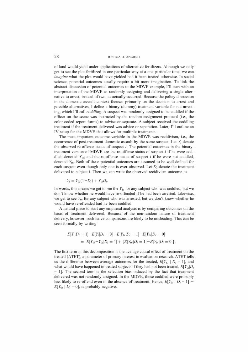
The most important outcome variable in the MDVE was recidivism, i.e., the
occurrence of post-treatment domestic assault by the same suspect. Let Yi denote
the observed re-offense status of suspect i. The potential outcomes in the binary-
treatment version of MDVE are the re-offense status of suspect i if he were cod-
dled, denoted Y1i, and the re-offense status of suspect i if he were not coddled,
denoted Y0i. Both of these potential outcomes are assumed to be well-defined for
each suspect even though only one is ever observed. Let Di denote the treatment
delivered to subject i. Then we can write the observed recidivism outcome as
Yi ¼ Y0i 1jDið Þ þ Y1iDi:
In words, this means we get to see the Y1i for any subject who was coddled, but we
don’t know whether he would have re-offended if he had been arrested. Likewise,
we get to see Y0i for any subject who was arrested, but we don’t know whether he
would have re-offended had he been coddled.
A natural place to start any empirical analysis is by comparing outcomes on the
basis of treatment delivered. Because of the non-random nature of treatment
delivery, however, such naive comparisons are likely to be misleading. This can be
seen formally by writing
E YijDi ¼ 1½ �jE YijDi ¼ 0½ � ¼E Y1ijDi ¼ 1½ �jE Y0ijDi ¼ 0½ �
¼ E Y1ijY0ijDi ¼ 1½ � þ E Y0ijDi ¼ 1½ �jE Y0ijDi ¼ 0½ �f g:
The first term in this decomposition is the average causal effect of treatment on the
treated (ATET), a parameter of primary interest in evaluation research. ATET tells
us the difference between average outcomes for the treated, E[Y1i | Di = 1], and
what would have happened to treated subjects if they had not been treated, E[Y0i|Di
= 1]. The second term is the selection bias induced by the fact that treatment
delivered was not randomly assigned. In the MDVE, those coddled were probably
less likely to re-offend even in the absence of treatment. Hence, E[Y0i | Di = 1] j
E[Y0i | Di = 0], is probably negative.
JOSHUA D. ANGRIST28

Selection bias disappears when delivered treatment is determined in a manner
independent of potential outcomes, as in a randomized trial with perfect com-
pliance. We then have
E YijDi ¼ 1½ �jE YijDi ¼ 0½ � ¼ E Y1ijY0ijDi ¼ 1½ � ¼ E Y1ijY0i½ �:
With perfect compliance, the simple treatment-control comparison recovers ATET.
Moreover, because {Y1i,Y0i} is assumed to be independent of Di in this case, ATET
is also the population average treatment effect, E[Y1i j Y0i].
The most important consequence of non-compliance is the likelihood of a
relation between potential outcomes and delivered treatments. This relation con-
founds analyses based on delivered treatments because of selection bias. But we
have an ace in the hole: the compliance problem does not compromise the
independence of potential outcomes and randomly assigned intended treatments.
The IV framework provides a set of simple strategies to convert comparisons using
intended random assignment, i.e., ITT effects, into consistent estimates of the causal
effect of treatments delivered.
The easiest way to see how IV solves the compliance problem is in the context
of a model with constant treatment effects, i.e., Y1i j Y0i = !, for some constant, !.
Also, let Y0i = " + "i, where " = E[Y0i]. The potential outcomes model can now
be written
Yi ¼ "þ !Di þ "i; ð1Þ
where ! is the treatment effect of interest. Note that because Di is a dummy
variable, the regression of Yi on Di is just the difference in mean outcomes by
delivered treatment status. As noted above, this difference does not consistently
estimate ! because Y0i and Di are not independent (equivalently, "i and Di are
correlated).
The random assignment of intended treatment status, which I"ll call Zi, provides
the key to untangling causal effects in the face of treatment dilution and migration.
By virtue of random assignment, and the assumption that assigned treatments have
no direct effect on potential outcomes other than through delivered treatments, Y0i
and Zi are independent. It therefore follows that
E "ijZi½ � ¼ 0; ð2Þ
though "i is not similarly independent of Di. Taking conditional expectations of
Equation (1) with Zi switched off and on, we obtain a simple formula for the
treatment effect of interest:
E Y ijZi ¼ 1� �
� E Y ijZi ¼ 0� �� ��
E DijZi ¼ 1� �
� E DijZi ¼ 0� �� �
¼ !:
ð3Þ
IV METHODS IN EXPERIMENTAL CRIMINOLOGICAL RESEARCH 29

Thus, the causal effect of delivered treatments is given by the causal effect of
assigned treatments (the ITT effect) divided by E[Di | Zi = 1]jE[Di | Zi = 0].
Note that in experiments where there is complete compliance in the comparison
group (i.e., no controls get treated), Formula (3) is just the ITT effect divided by
the compliance rate in the originally assigned treatment group. More generally, the
denominator in Equation (3) is the difference in compliance rates by assignment
status. In the MDVE, E[Di | Zi = 1] = P[Di = 1 | Zi = 1] = .77, that is, a little over
three-fourths of those assigned to be coddled were coddled. On the other hand,
almost no one assigned to be arrested was coddled:
E DijZi ¼ 0½ � ¼ P½Di ¼ 1jZi ¼ 0� ¼ :01:
Hence, the denominator of Equation (3) is estimated to be about .76. The sample
analog of Formula (3) is called a Wald estimator, since this formula first appeared
in a paper by Wald (1940) on errors-in-variables problems. The law of large
numbers, which says that sample means converge in probability to population
means, ensures that the Wald estimator of ! is consistent (i.e., converges in
probability to !).4
The constant-effects assumption is clearly unrealistic. We`d like to allow for the
fact that some men change their behavior in response to coddling, while others are
affected little or not at all. There is also important heterogeneity in treatment de-
livery. Some suspects would have been coddled with or without the experimental
manipulation, while others were coddled only because the police were instructed to
treat them this way. The MDVE is informative about causal effects only on this
latter group.
Imbens and Angrist (1994) showed that in a world of heterogeneous treatment
effects, IV methods capture the average causal effect of delivered treatments on the
subset of treated men whose delivered treatment status can be changed by the
random assignment of intended treatment status. The men in this group are called
compliers, a term introduced in the IV context by Angrist et al. (1996). In a
randomized drug trial, for example, compliers are those who Ftake their medicine_when randomly assigned to do so, but not otherwise. In the MDVE, compliers were
coddled when randomly assigned to be coddled but would not have been coddled
otherwise.
The average causal effect for compliers is called a local average treatment effect
(LATE). A formal description of LATE requires one more bit of notation. Define
potential treatment assignments, D0i and D1i, to be individual i`s treatment status
when Zi equals 0 or 1. Note that one of D0i or D1i is necessarily counterfactual
since observed treatment status is
Di ¼ D0i þ Zi D1ijD0ið Þ: ð4Þ
In this setup, the key assumptions supporting causal inference are: (1) conditional
independence, i.e., that the joint distribution of {Y1i, Y0i, D1i, D0i} is independent of
Zi; and, (2) monotonicity, which requires that either D1i Q D0i for all i or vice versa.
JOSHUA D. ANGRIST30

Assume without loss of generality that monotonicity holds with D1i Q D0i.
Monotonicity requires that, while the instrument might have no effect on some
individuals, all of those affected are affected in the same way. Monotonicity in the
MDVE amounts to assuming that random assignment to be coddled can only make
coddling more likely, an assumption that seems plausible. Given these two iden-
tifying assumptions, the Wald estimator consistently estimates LATE, which is
written formally as E[Y1ijY0i | D1i 9 D0i].5
Compliers are those with D1i 9 D0i, i.e., they have D1i = 1 and D0i = 0. The
monotonicity assumption partitions the world of experimental subjects into three
groups: compliers who are affected by random assignment and two unaffected
groups. The first unaffected group consists of always-takers, i.e., subjects with
D1i = D0i = 1. The second unaffected group consists of never-takers, i.e., subjects
with D1i = D0i = 0. Because the treatment status of always-takers and never-takers
is invariant to random assignment, IV estimates are uninformative about treatment
effects for subjects in these groups.
In general, LATE is not the same as ATET, the average causal effect on all
treated individuals. Equation (4) shows that the treated can be divided into two
groups: the set of subjects with D0i = 1, and the set of subjects with D0i = 0, D1i = 1,
and Zi = 1. Subjects in the first set, with D0i = 1, are always-takers since D0i = 1
implies D1i = 1 by monotonicity. The second set consists of compliers with Zi = 1.
By virtue of the random assignment of Zi, the average causal effect on compliers
with Zi = 1 is the same as the average causal effects for all compliers. In general,
therefore, ATET differs from LATE because it is a weighted average of two
effects: one on always-takers and one on compliers.
An important special case when LATE equals ATET is when D0i equals zero
for everybody, i.e., there are no always-takers. This occurs in randomized trials
with one-sided non-compliance, a scenario that typically arises because no one in
the control group receives treatment. If no one in the control group receives
treatment, then by definition there can be no always-takers. Hence, all treated
subjects must be compliers. The MDVE is (approximately) this sort of experiment.
Since we have defined treatment as coddling, and (almost) no one in the group
assigned to be arrested was coddled, there are (almost) no always-takers. LATE in
this case is therefore ATET, the effect of coddling on the population coddled.6
The language of 2SLS
Applied economists typically discuss IV using the language of two-stage least
squares (2SLS), a generalized IV estimator introduced by Theil (1953) in the
context of simultaneous equation models. In models without covariates, the 2SLS
estimator using a dummy instrument is the same as the Wald estimator. In models
with exogenous covariates, 2SLS provides a simple and easily implemented
generalization that also allows for multiple instruments and multiple treatments.
Suppose the setup is the same as before, with the modification that we’d now
like to control for a vector of covariates, Xi. In particular, suppose that if Di had
IV METHODS IN EXPERIMENTAL CRIMINOLOGICAL RESEARCH 31

been randomly assigned as intended, we’d be interested in a regression-adjusted
treatment effect computed by ordinary least squares (OLS) estimation of the
equation:
Yi ¼ Xi
0"þ !Di þ "i: ð5Þ
In 2SLS language, Equation (5) is the structural equation of interest. Note that the
causal effect in this model is the effect of being coddled on recidivism, relative to
the baseline recidivism rate when arrested.
The two most likely rationales for including covariates in Equation (5) are: (1)
that treatment was randomly assigned conditional on these covariates, and, (2) a
possible statistical efficiency gain (i.e., reduced sampling variance). In the MDVE,
for example, the coddling treatment might have been randomly assigned with
higher probability to suspects with no prior history of assault. We_d then need to
control for assault history in the IV analysis. Efficiency gains are a consequence of
the fact that regression standard errors Y whether 2SLS or OLS Y are proportional
to the variance of the residual, "i. The residual variance is typically reduced by the
covariates, as long as the covariates have some power to predict outcomes.7
In principle, we can construct 2SLS estimates in two steps, each involving an
OLS regression. In the first stage, the endogenous right-hand side variable (treat-
ment delivered in the MDVE) is regressed on the Fexogenous_ covariates plus the
instrument (or instruments). This regression can be written
Di ¼ X ¶i:0 þ :1Zi þ )i: ð6Þ
The coefficient on the instrument in this equation, :1, is called the Ffirst-stage
effect_ of the instrument. Note that the first-stage equation must include exactly the
same exogenous covariates as appear in the structural equation.8 The size of the
first-stage effect is a major determinant of the statistical precision of IV estimates.
Moreover, in a model with dummy endogenous variables like the treatment dum-
my analyzed here, the first-stage effect measures the proportion of the population
that are compliers.9
In the second stage, fitted values from the first-stage are plugged directly into
the structural equation in place of the endogenous regressor. Note, however, that
although the term 2SLS arises from the fact that 2SLS estimates can be constructed
from two OLS regressions, we don’t usually compute them this way. This is
because the resulting standard errors are incorrect. Best practice therefore is to use
a packaged 2SLS routine such as may be found in software like SAS or Stata.
In addition to the first-stage, an important auxiliary equation that is often dis-
cussed in the context of 2SLS is the reduced form. The reduced form for Yi is the
regression obtained by substituting the first-stage into the causal model for Yi, in
this case, Equation (5). In the MDVE, we can write the reduced form as
Yi¼ X 0i"þ ! X 0i:0 þ :1Zi þ )i
� �þ "i
¼ X 0i %0 þ %1Zi þ vi:
ð7Þ
JOSHUA D. ANGRIST32

The coefficient %1 is said to be the Freduced-form effect_ of the instrument. Like the
first stage, the reduced form parameters can estimated by OLS, i.e., by simply
running a regression.
Note that with a single endogenous variable and a single instrument, the effect
of Di in the causal model is the ratio of reduced-form to first-stage effects:
! ¼ %1=:1:
2SLS second-stage estimates can therefore be understood as a re-scaling of the
reduced form. It can also be shown that the significance levels for the reduced-form
and the second-stage in this model are asymptotically the same under the null
hypothesis of no treatment effect. Hence, the workingman’s IV motto: BIf you
can’t see your causal effect in the reduced form, it ain’t there.[On final reason for looking at the reduced form is that Y in contrast with the
2SLS estimates themselves Y the reduced form estimates have all the attractive
statistical properties of any ordinary least squares regression estimates. In
particular, estimates of reduced form regression coefficients are unbiased (i.e.,
centered on the population parameter in repeated samples) and the theory that
justifies statistical inference for these coefficients (i.e., confidence intervals and
hypothesis testing) does not require large samples. 2SLS estimates on the other
hand, are not unbiased, although they are consistent. This means that in large
samples, the estimates can be expected to be close to the target population
parameter, though in small samples, they can be unreliable. Moreover, the
statistical theory that justifies confidence intervals and hypothesis testing for 2SLS
requires that samples be large enough for a reasonably good asymptotic
approximation (in particular, for application of central limit theorems).
How large a sample is large enough for asymptotic statistical theory to work?
Unfortunately, there is no general answer to this question. Various theoretical
arguments and simulations studies have shown, however, that the asymptotic
approximations used for 2SLS inference are usually reasonably accurate in models
where the number of instruments is equal to (or not much more than) the number
Table 2. First stage and reduced forms for Model 1.
Endogenous variable is coddled
First stage Reduced form (ITT)
(1) (2)* (3) (4)*
Coddled-assigned 0.786 (0.043) 0.773 (0.043) 0.114 (0.047) 0.108 (0.041)
Weapon j0.064 (0.045) j0.004 (0.042)
Chem. influence j0.088 (0.040) 0.052 (0.038)
Dep. var. mean 0.567
(CoddledYdelivered)
0.178
(Re-arrested)
The table reports OLS estimates of the first-stage and reduced form for Model 1 in the text.
*Other covariates include year and quarter dummies, and dummies for non-white and mixed race.
IV METHODS IN EXPERIMENTAL CRIMINOLOGICAL RESEARCH 33

of endogenous variables (as would be the case in studies using randomly assigned
intention to treat as an instrument for treatment delivered). Also, that the key to
valid inference is a reasonably strong first stage, with a t-statistic for the coefficient
on the instrumental variable in the first-stage equation of at least 3. For further
discussion of statistical inference with 2SLS, see Angrist and Krueger (2001).
2SLS Estimates for MDVE with one endogenous variable
The first-stage effect of being assigned to the coddling treatment is .79 in a model
without covariates and .77 in a model that controls for a few covariates.10 These
first-stage effects can be seen in the first two columns of Table 2, which report
estimates of Equation (6) for the MDVE. The reduced form effects of random
assignment to the coddling treatment, reported in columns 3 and 4, are about .11,
and significantly different from zero with standard errors of .041Y.047. The first-
stage and reduced-form estimates change little when covariates are added to the
model, as expected since Zi was randomly assigned. The 2SLS results derived from
these first-stage and reduced form estimates are reported in Table 3.
Before turning to a detailed discussion of the 2SLS results, one caveat is in
order: for simplicity, I discuss these estimates as if they were constructed in the
usual way, i.e., by estimating Equations (5), (6), and (7) using micro-data. In
reality, however, I was unable to locate or construct the original recidivism var-
iable from the MDVE public-use data sets (Berk and Sherman, 1993). I therefore
generated my own micro-data on recidivism from the Logit coefficients reported
in Berk and Sherman (1988, Tables 4 and 6). Note that the Logistic regression,
of, say Yi on Di implicitly determines the conditional mean of Yi given Di (by
inverting the logistic transformation of fitted values, a simple mathematical
operation). Because Yi in this case is a dummy variable, this conditional mean is
also the conditional distribution of Yi given Di. It is therefore straightforward to
construct, by sampling from this distribution, a sample with same joint distribution
of Yi and Di (or Yi and Zi) as must have appeared in Berk and Sherman’s original
data set.
Table 3. OLS and 2SLS estimates for Model 1.
Endogenous variable is coddled
OLS IV/2SLS
(1) (2)* (3) (4)*
CoddledYdelivered 0.087 (0.044) 0.070 (0.038) 0.145 (0.060) 0.140 (0.053)
Weapon 0.010 (0.043) 0.005 (0.043)
Chem. influence 0.057 (0.039) 0.064 (0.039)
The Table reports OLS and 2SLS estimates of the structural equation in Model 1.
*Other covariates include year and quarter dummies, and dummies for non-white and mixed race.
JOSHUA D. ANGRIST34
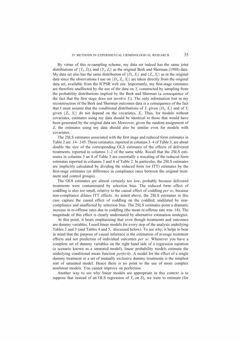
By virtue of this re-sampling scheme, my data set indeed has the same joint
distributions of {Yi, Di), and {Yi, Zi} as the original Berk and Sherman (1988) data.
My data set also has the same distribution of {Di, Xi} and {Zi, Xi} as in the original
data since the observations I use on {Di, Zi, Xi} are taken directly from the original
data set, available from the ICPSR web site. Importantly, my first-stage estimates
are therefore unaffected by the use of the data on Yi constructed by sampling from
the probability distributions implied by the Berk and Sherman (a consequence of
the fact that the first stage does not involve Yi). The only information lost in my
reconstruction of the Berk and Sherman outcomes data is a consequence of the fact
that I must assume that the conditional distributions of Yi given {Di, Xi} and of Yi
given {Zi, Xi} do not depend on the covariates, Xi. Thus, for models without
covariates, estimates using my data should be identical to those that would have
been generated by the original data set. Moreover, given the random assignment of
Z, the estimates using my data should also be similar even for models with
covariates.
The 2SLS estimates associated with the first stage and reduced form estimates in
Table 2 are .14Y.145. These estimates, reported in columns 3Y4 of Table 3, are about
double the size of the corresponding OLS estimates of the effects of delivered
treatments, reported in columns 1Y2 of the same table. Recall that the 2SLS esti-
mates in columns 3 an 4 of Table 3 are essentially a rescaling of the reduced form
estimates reported in columns 3 and 4 of Table 2. In particular, the 2SLS estimates
are implicitly calculated by dividing the reduced form (or ITT) estimates by the
first-stage estimates (or difference in compliance rates between the original treat-
ment and control groups).
The OLS estimates are almost certainly too low, probably because delivered
treatments were contaminated by selection bias. The reduced form effect of
coddling is also too small, relative to the causal effect of coddling per se, because
non-compliance dilutes ITT effects. As noted above, the 2SLS estimates in this
case capture the causal effect of coddling on the coddled, undiluted by non-
compliance and unaffected by selection bias. The 2SLS estimates point a dramatic
increase in re-offense rates due to coddling (the mean re-offense rate was .18). The
magnitude of this effect is clearly understated by alternative estimation strategies.
At this point, it bears emphasizing that even though treatments and outcomes
are dummy variables, I used linear models for every step of the analysis underlying
Tables 2 and 3 (and Tables 4 and 5, discussed below). To see why, it helps to bear
in mind that the purpose of causal inference is the estimation of average treatment
effects and not prediction of individual outcomes per se. Whenever you have a
complete set of dummy variables on the right hand side of a regression equation
(a scenario known as a saturated model), linear probability models estimate the
underlying conditional mean function perfectly. A model for the effect of a single
dummy treatment or a set of mutually exclusive dummy treatments is the simplest
sort of saturated model. Hence there is no point to the use of more complex
nonlinear models. You cannot improve on perfection.
Another way to see why linear models are appropriate in this context is to
suppose that instead of an OLS regression of Yi on Di, we were to estimate (for
IV METHODS IN EXPERIMENTAL CRIMINOLOGICAL RESEARCH 35
example) the corresponding Probit regression. The Probit conditional mean
function in this case is E[Yi | Di] = 6[.0 + .1Di], where 6[�] is the Normal
distribution function. But since Di is a dummy variable, this conditional mean
function can be rewritten as a linear model:
E YijDi½ � ¼ 6 .0½ � þ 6 .0 þ .1� � 6½.0�½ ÞDi:ð
Thus, the Probit estimate of the effect of Di is 6[.0 + .1] j 6[.0]). But since the
conditional mean function is linear in Di, this is exactly what the OLS regression of
Yi on Di, will produce. In other words, the slope coefficient in the OLS regression
will equal 6[.0 + .1] j 6[.0]. In fact, all two-parameter models will generate the
same marginal effect of Di.
In more complicated models with additional covariates, some of which are not
dummy variables, or when the model is not fully saturated, it is no longer the case
that Probit and OLS will produce exactly the same treatment effects (again, it’s
worth emphasizing that it is these effects that are of interest; the Probit coefficients
themselves mean little). But in practice, the treatment effects generated by
nonlinear models are likely to be indistinguishable from OLS regression
coefficients. See, for example, the comparison of Probit and regression estimates
in Angrist (2001). This close relation is a consequence of a very general regression
property Y no matter what the shape of the conditional mean function you are
trying to estimate, OLS regression always provides the minimum mean square
approximation to it (see, e.g., Goldberger, 1991).
The case for using 2SLS to estimate linear probability models with dummy
endogenous variables is slightly more involved than the case for using OLS
regression to estimate models without endogenous variables. Nevertheless, the
argument is essentially similar: even with binary outcomes like recidivism, linear
2SLS estimates have a robust causal interpretation that is insensitive to the possible
nonlinearity induced by dummy dependent variables. For example, the interpre-
tation of IV as estimating LATE is unaffected by the fact that the outcome is a
dummy. Likewise, consistency of 2SLS estimates is unaffected by the possible
nonlinearity of the first-stage conditional expectation function, E[Di | Xi, Zi]. For
details, see Angrist (2001), which also offers some simple nonlinear alternatives
for those who insist.11
2SLS estimates with two endogenous variables
The analysis so far looks at the MDVE as if it involved a single treatment. I now
turn to a 2SLS model that more realistically allows for distinct causal effects for
the two types of coddling that were randomly assigned, separation and advice. A
natural generalization of Equation (5) incorporating distinct causal effects for these
two interventions is
Y i ¼ X 0i"þ !aDai þ !sDsi þ "i; ð8Þ
JOSHUA D. ANGRIST36

where Dai and Dsi are dummies that indicate delivery of advice and separation. As
before, because of the endogeneity of delivered treatments, OLS estimates of
Equation (8) are likely to be misleading. Again, the causal effects of interest are
the effects of advice and separation relative to the baseline recidivism rate when
arrested. The potential outcomes that motivate Equation (8) as a causal model
describe each suspect’s recidivism status had he been assigned to one of three
possible treatments (arrest, advise, separate).
Equation (8) is a structural model with two endogenous regressors, Dai and Dsi.
We also have two possible instruments, Zai and Zsi, dummy variables indicating
random assignment to advice and separation as intended treatments. The cor-
responding first-stage equations are
Dai ¼ X 0i :0a þ :aaZai þ :asZsi þ �ai ð9aÞ
Dsi ¼ X 0i :0s þ :saZai þ :ssZsi þ �si; ð9bÞ
where :aa and :as are the first-stage effects of the two instruments on delivered
advice, Dai, and :sa and :ss are the first-stage effects of the two instruments on
delivered separation, Dsi.
The reduced form equation for this two-endogenous-variables setup is obtained
by substituting Equations (9a) and (9b) into Equation (8). Similarly, the second
stage is obtained by substituting fitted values from the first stages into the structural
equation.12 Note that in a model with two endogenous variables we must have at
least two instruments for the second stage estimates to exist.13 Assuming the
second stage estimates exist, which is equivalent to saying that the structural
equation is identified, the 2SLS estimates in this case can be interpreted as
capturing the covariate-adjusted causal effects of each delivered treatment on those
who comply with random assignment.
Random assignment to receive advice increased the likelihood of advice
delivery by .78. Assignment to the separation treatment also increased the
likelihood of receiving advice, but this effect is small and not significantly
different from zero. These results can be seen in columns 1Y2 of Table 4, which
report the estimates of first-stage effects from Equation (9a). The corresponding
estimates of Equation (9b), reported in columns 3Y4 of the table, show that
assignment to the separation treatment increased delivered separation rates by
about .72, while assignment to advice had almost no effect on the likelihood of
receiving the separation treatment. The reduced form effects of random assignment
to receive advice range from .088Y.097, while the reduced form estimates of ran-
dom assignment to be separated are about .13. The reduced form estimates are
reported in columns 5Y6 of the table.
OLS and 2SLS estimates of the two-endogenous-variables model are reported in
Table 5. Interestingly, the OLS estimates of the effect of delivered advice on re-
offense rates are small and not significantly different from zero. The OLS estimates
of the effect of being separated are much larger and significant. Both of these
IV METHODS IN EXPERIMENTAL CRIMINOLOGICAL RESEARCH 37

results are reported in columns 1Y2 of the table. In contrast with the OLS effects,
the 2SLS estimates of the effects of both types of treatment are substantial and at
least marginally significant. For example, the 2SLS estimate of the impact of the
advice intervention is .107 (SE = .059) in a model with covariates. The 2SLS
estimate of the impact of separation is even larger, at around .17.
As in the model with a single endogenous variable, the reduced-form estimates
of intended treatment effects are larger than the corresponding OLS estimates of
Table 4. First stage and reduced forms for Model 2.
Two endogenous variables: Advise, separate
First stages
Reduced form (ITT)Advised Separated
(1) (2)* (3) (4)* (5) (6)*
Advise-
assigned
0.778
(0.039)
0.766 (0.039) 0.035
(0.043)
0.035 (0.043) 0.097
(0.054)
0.088 (0.046)
Separate-
assigned
0.044
(0.038)
0.031 (0.039) 0.717
(0.042)
0.715 (0.043) 0.130
(0.053)
0.127 (0.046)
Weapon j0.038 (0.036) j0.031 (0.039) j0.001 (0.042)
Chem.
influence
j0.068 (0.032) j0.018 (0.035) 0.051 (0.038)
Dep. var.
mean
0.283
(Adv.-deliver)
0.283
(Sep.-deliver)
0.178
(Re-arrested)
The table reports OLS estimates of the first-stage and reduced form for Model 2 in the text.
*In addition to the covariates reported in the table, these models include year and quarter dummies, and
dummies for non-white and mixed race.
Table 5. OLS and 2SLS estimates for Model 2.
Two endogenous variables: Advise, separate
OLS IV/2SLS
(1) (2)* (3) (4)*
Advise-assigned 0.047 (0.052) 0.019 (0.046) 0.116 (0.068) 0.107 (0.059)
Separate-assigned 0.126 (0.052) 0.120 (0.046) 0.174 (0.073) 0.174 (0.063)
Weapon 0.015 (0.043) 0.008 (0.043)
Chem. influence 0.052 (0.039) 0.061 (0.039)
Test F = 1.87 F = 4.14 F = .64 F = 1.14
Advise = separate p = .170 p = .043 p = .420 p = .290
The Table reports OLS and 2SLS estimates of the structural equation in Model 2.
*In addition to the covariates reported in the table, these models include year and quarter dummies, and
dummies for non-white and mixed race.
JOSHUA D. ANGRIST38

delivered treatment effects, and the 2SLS estimates are larger than the cor-
responding reduced forms. The gap between OLS and 2SLS is especially large for
the advice effects, suggesting that the OLS estimates of the effect of receiving
advice are more highly contaminated by selection bias than the OLS estimates of
the effect of separation. Moreover, the difference between the separation and ad-
vice treatment effects is much larger when estimated by 2SLS than in the reduced
form.
Does anything new come out of this IV analysis of the MDVE? Two findings
seem important. First, a comparison of 2SLS estimates with estimates that ignore
the endogeneity of treatment delivered indicate considerable selection bias in the
latter. In particular, the 2SLS estimates of the effect of coddling are about twice as
large as the corresponding OLS estimates, largely due to the fact that the suspects
who were coddled were those least likely to re-offend anyway. The IV framework
corrects for this important source of bias. A related point is that the ITT effects Yequivalently, the 2SLS reduced form estimates Y are not a fair comparison for
gauging selection bias. Although ITT effects have a valid causal interpretation (i.e.,
they preserve random assignment), they are diluted by non-compliance. OLS es-
timates of the effect for treatment delivered, while contaminated by selection bias,
are not similarly diluted. The second major finding, and one clearly related to the
first, is that non-compliance was important enough to matter; in some cases, the
2SLS estimates are as much as one-third larger than the corresponding ITT effects.
Based on these results, the evidence for a deterrent effect of arrest is even stronger
than previously believed.
Models with variable treatment intensity and observational studies
In closing, it bears emphasizing that IV methods are not limited to the estimation
of the effects of binary on-or-off treatments like coddling, separation, or advice in
the MDVE. Many experimental evaluations are concerned with the effects of in-
terventions with variable treatment intensity, i.e., the effects of an endogenous
variable that takes on ordered integer values. Applications of IV to these sorts of
interventions include Krueger’s (1999) analysis of experimental estimates of the
effects of class size, the Permutt and Hebel (1989) study of an experiment to
reduce the number of cigarettes smoked by pregnant women, and the Powers and
Swinton (1984) randomized study of the effect of hours of preparation for the GRE
test.
The studies mentioned above use 2SLS or related IV methods to analyze data
from randomized trials where the treatment of interest takes on values like 0, 1, 2,
. . . (cigarettes, hours of study) or 15, 16, 17 . . . (class size). Although these papers
interpret IV estimates using traditional constant-effects models, the 2SLS estimates
they report also have a more general LATE interpretation. In particular, 2SLS
estimates of models with variable treatment intensity give the average causal
response for compliers along the length of the underlying causal response function.
See Angrist and Imbens (1995) for details.
IV METHODS IN EXPERIMENTAL CRIMINOLOGICAL RESEARCH 39
The IV framework also goes beyond randomized trials and can be used to
exploit quasi-experimental variation in observational studies. An example from my
own work is Angrist (1990), which uses the draft lottery numbers that were ran-
domly assigned in the early 1970s as instrumental variables for the effect of Viet-
nam-era veteran status on post-service earnings. Draft lottery numbers are highly
correlated with veteran status among men born in the early 1950s, and probably
unrelated to earnings for any other reason.
A second example from my portfolio illustrates the fact that instrumental
variables need not be randomly assigned to be useful.14 Angrist and Lavy (1999)
constructed instrumental variables estimates of the effects of class size on test
scores. The instrument in this case is the class size predicted using Maimonides
rule, a mathematical formula derived from the practice in Israeli elementary
schools of dividing grade cohorts by integer multiples of 40, the maximum class
size (the same rule proposed by Maimonides in his Mishneh Torah biblical
commentary). This study can be seen as an application of Campbell’s (1969)
celebrated regression-discontinuity design for quasi-experimental research, but
also as a type of IV. The extension of IV methods to quasi-experimental
criminological research designs seems an especially promising avenue for further
work.
Acknowledgements
Special thanks to Richard Berk, Howard Bloom, David Weisburd, and the par-
ticipants in the May 2005 Jerry Lee Conference for the stimulating discussions that
led to this paper. Thanks also to the editor and three anonymous reviewers for
helpful comments.
Notes
1 Social experiments in labor economics, which are never double or even single-blind,
often allow those selected for treatment to opt out (an example is the Illinois
unemployment insurance bonuses experiment; see Woodbury and Spiegelman 1987).
And even in double-blind clinical trials, clinicians sometimes decipher and change
treatment assignments (Schultz 1995).2 My brief discussion here glosses over a number of technical details. For a more
comprehensive introduction to IV see Angrist and Krueger (2001, 1999), or the chapters
on IV in Wooldridge (2003).3 The fact that those who comply with randomly assigned treatments are not randomly
selected can be seen in medical trials, where subjects who comply with protocol by
taking a randomly assigned experimental treatment with no clinical effects Y i.e., a
placebo Y are often healthier than those who don_t (as in the study analyzed by Efron and
Feldman 1991). Efron and Feldman use the placebo sample in an attempt to characterize
those who comply with treatment assignment directly, but placebo-controlled trials are
JOSHUA D. ANGRIST40

unusual in social science. Luckily, however, at least as far as solving the compliance
problem goes, they are unnecessary.4 An estimator is said to be consistent when the limit (as a function of sample size) of the
probability that it is close to the population parameter being estimated is 1. In other
words, a consistent estimate can be taken to be close to the parameter of interest in large
samples. Note that consistency is not the same as unbiasedness; an unbiased estimator
has a sampling distribution centered on the parameter of interest in a sample of any size.
I briefly discuss this point further below.5 In econometrics, a parameter is said to be Fidentified_ when it can be constructed from
the joint distribution of observed random variables. Assumptions that allow a parameter
to be identified are called Fidentifying assumptions._ The identifying assumptions for IV,
independence and monotonicity, allow us to construct LATE from the joint distribution
of {Yi, Di, Zi}.6 The fact that a randomized trial with one-sided non-compliance can be used to estimate
the effect of treatment on the treated was first noted by Bloom (1984).7 The causal (LATE) interpretation of IV estimates is similar in models with and without
covariates. See Angrist and Imbens (1995) or Abadie (2003) for details.8 If the first stage includes covariates omitted from the second stage, then the covariates
are, in fact, playing the role of instruments. If, on the other hand, covariates included in
the second stage are omitted from the first stage, then the first stage residuals, which
necessarily end up in the second stage error term, are correlated with the covariates,
biasing the second-stage estimates. See e.g., Wooldridge (2003).9 Formally, this is because without covariates, E[D1ijD0i] = :1. With covariates,
E[D1ijD0i | Xi] = :1 if the first stage is linear and additive in covariates, and, more
generally, E{E[D1ijD0i | Xi]} � :1.10 The covariates are dummies for the presence of a weapon and whether the suspect was
under chemical influence, year and quarter dummies for time of follow-up, and dummies
for suspects_ race (non-white and mixed).11 Rossi et al. (1980) present an IV-type analysis of a stipend program for ex-offenders.
Their analysis deviates from an orthodox 2SLS procedure in a number of respects,
however. First, they include potentially endogenous outcome variables on the right-hand
side as if these were covariates. Second, they use nonlinear models (e.g., Tobit) to which
IV methods do not easily transfer and which are, in any case, not well-suited to the sort
of question they are addressing.12 With multiple endogenous variables, the second stage estimates can no longer be obtained
as the ratio of reduced form to first-stage coefficients, but rather solve a matrix equation.
Again, the best strategy for real empirical work is to use packaged 2SLS software.13 The second stage has a regression design matrix with number of columns equal to
dim(Xi) + 2. This matrix must be of full column rank for the second stage to exist. The
rank of the design matrix is equal to the number of linearly independent columns in the
matrix. This can be no more than dim(Xi) plus the number of instruments, since the fitted
values used in the second step are linear combinations of Xi and the instruments. Hence
the need for at least K instruments when there are K endogenous variables.14 A pioneering illustration of this point from criminology is Levitt_s (1997) study of the
effects of extra policing using municipal election cycles to create instruments for
numbers of police. See also McCrary (2002), who discusses a technical problem with
Levitt_s original analysis. Recent applications of IV in criminology include Snow-Jones
and Gondolf (2002), Gottfredson (2005), and White (2005).
IV METHODS IN EXPERIMENTAL CRIMINOLOGICAL RESEARCH 41

References
Abadie, A. (2003). Semiparametric instrumental variable estimation of treatment response
models. Journal of Econometrics 113(2), 231Y263.
Angrist, J. D. (1990). Lifetime earnings and the Vietnam era draft lottery: Evidence from
social security administrative records. American Economic Review 80(3), 313Y335.
Angrist, J. D. (2001). Estimation of limited dependent variable models with dummy
endogenous regressors: Simple strategies for empirical practice. Journal of Business and
Economic Statistics 19(1), 2Y16.
Angrist, J. D. & Imbens, G. W. (1995). Two-stage least squares estimates of average causal
effects in models with variable treatment intensity. Journal of the American Statistical
Association 90(430), 431Y442.
Angrist, J. D. & Krueger, A. B. (1999). Empirical strategies in labor economics. In O.
Ashenfelter & D. Card (Eds.), Handbook of labor economics, Volume IIIA ( pp.
1277Y1366). Amsterdam: North-Holland.
Angrist, J. D. & Krueger, A. B. (2001). Instrumental variables and the search for
identification. Journal of Economic Perspectives 15(4), 69Y86.
Angrist, J. D. & Lavy, V. C. (1999). Using Maimonides’ rule to estimate the effect of class
size on student achievement. Quarterly Journal of Economics 114(2), 533Y575.
Angrist, J. D. & Lavy, V. C. (2002). The effect of high school matriculation awards YEvidence from randomized trials,[ NBER Working Paper 9389, December.
Angrist, J. D., Imbens, G. W. & Rubin, D. B. (1996). Identification of causal effects using
instrumental variables. Journal of the American Statistical Association 91(434), 444Y455.
Berk, R. A. & Sherman, L. W. (1988). Police response to family violence incidents: An
analysis of an experimental design with incomplete randomization. Journal of the
American Statistical Association 83(401), 70Y76.
Berk, R. A. & Sherman, L. W. (1993). Specific Deterrent Effects Of Arrest For Domestic
Assault: Minneapolis, 1981Y1982 [Computer file]. Conducted by the Police Foundation.
2nd ICPSR ed. Ann Arbor, Michigan: Inter-university Consortium for Political and Social
Research [producer and distributor].
Berk, R. A., Smyth, G. K. & Sherman, L. W. (1988). When random assignment fails: Some
lessons from the Minneapolis spouse abuse experiment. Journal of Quantitative
Criminology 4(3), 209Y223.
Bloom, H. S. (1984). Accounting for no-shows in experimental evaluation designs.
Evaluation Review 8(2), 225Y246.
Boruch, R., De Moya, D. & Snyder, B. (2002). The importance of randomized field trials in
education and related areas. In F. Mosteller & R. Boruch (Eds.), Evidence matters:
randomized trials in education research. Washington, DC: Brookings Institution.
Campbell, D. T. (1969). Reforms as experiments. American Psychologist 24, 409Y429.
Cook, T. D. (2001). Sciencephobia: Why education researchers reject randomized experi-
ments, Education Next http://www.educationnext.org), Fall, 63Y68.
Efron, B. & Feldman, D. (1991). Compliance as an explanatory variable in clinical trials.
Journal of the American Statistical Association 86(413), 9Y17.
Farrington, D. P. (1983). Randomized experiments on crime and justice. In M. H. Tonry &
N. Morris (Eds.), Crime and justice. Chicago: University of Chicago Press.
Farrington, D. P. & Welsh, B. C. (2005). Randomized experiments in criminology: What
have we learned in the last two decades? Journal of Experimental Criminology 1, 9Y38.
JOSHUA D. ANGRIST42

Gartin, P. R. (1995). Dealing with design failures in randomized field experiments: Analytic
issues regarding the evaluation of treatment effects. Journal of Research in Crime and
Delinquency 32(4), 425Y445.
Goldberger, A. S. (1991). A course in econometrics. Cambridge, MA: Harvard University
Press.
Gottfredson, D. C. (2005). Long-term Effects of Participation in the Baltimore City Drug
Treatment Court: Results from an Experimental Study,[ University of Maryland,
Department of Criminology and Criminal Justice,[ mimeo, October 2005.
Holland, P. W. (1986). Statistics and causal inference. Journal of the American Statistical
Association 81(396), 945Y970.
Imbens, G. W. & Angrist, J. D. (1994). Identification and estimation of local average
treatment effects. Econometrica 62(2), 467Y475.
Krueger, A. B. (1999). Experimental estimates of education production functions. Quarterly
Journal of Economics 114(2), 497Y532.
Levitt, S. D. (1997). Using electoral cycles in police hiring to estimate the effects of police
on crime. American Economic Review 87(3), 270Y290.
McCrary, J. (2002). Using electoral cycles in police hiring to estimate the effects of police
on crime: comment. American Economic Review 92(4), 1236Y1243.
Permutt, T. & Richard Hebel, J. (1989). Simultaneous-equation estimation in a clinical trial
of the effect of smoking on birth weight. Biometrics 45(2), 619Y622.
Powers, D. E. & Swinton, S. S. (1984). Effects of self-study for coachable test item types.
Journal of Educational Psychology 76(2), 266Y278.
Rezmovic, E. L., Cook, T. J. & Douglas Dobson, L. (1981). Beyond random assignment:
Factors affecting evaluation integrity. Evaluation Review 5(1), 51Y67.
Rossi, P. H., Berk, R. A. & Lenihan, K. J. (1980). Money, work, and crime: Experimental
evidence. New York: Academic.
Rubin, D. B. (1974). Estimating causal effects of treatments in randomized and non-
randomized studies. Journal of Educational Psychology 66, 688Y701.
Rubin, D. B. (1977). Assignment to a treatment group on the basis of a covariate. Journal of
Educational Statistics 2, 1Y26.
Sherman, L. W. & Berk, R. A. (1984). The specific deterrent effects of arrest for domestic
assault. American Sociological Review 49(2), 261Y272.
Snow Jones, A. & Gondolf, E. (2002). Assessing the effect of batterer program completion
on reassault: An instrumental variables analysis. Journal of Quantitative Criminology 18,
71Y98.
Theil, H. (1953). Repeated least squares applied to complete equation systems. The Hague:
Central Planning Bureau.
Wald, A. (1940). The fitting of straight lines if both variables are subject to error. Annals of
Mathematical Statistics 11, 284Y300.
Weisburd, D. L. (2003). Ethical practice and evaluation of interventions in crime and justice:
The moral imperative for randomized trials. Evaluation Review 27(3), 336Y354.
Weisburd, D. L., Lum, C. & Petrosino, A. (2001). Does research design affect study
outcomes in criminal justice? Annals of the American Academy of Political and Social
Science 578(6), 50Y70.
White, M. J. (2005). Acupuncture in Drug Treatment: Exploring its Role and Impact on
Participant Behavior in the Drug Court Setting, John Jay College of Criminal Justice, City
University of New York, mimeo.
IV METHODS IN EXPERIMENTAL CRIMINOLOGICAL RESEARCH 43

Woodbury, S. A. & Spiegelman, R. G. (1987). Bonuses to workers and employers to reduce
unemployment: Randomized trials in Illinois. American Economic Review 77(4),
513Y530.
Wooldridge, J. (2003). Introductory econometrics: A modern approach. Cincinnati, OH:
Thomson South-Western.
About the author
Joshua Angrist is a Professor of Economics at MIT and a Research Associate in the
NBER’s programs on Children, Education, and Labor Studies. A dual U.S. and Israeli
citizen, he taught at the Hebrew University of Jerusalem before coming to MIT. He holds a
B.A. from Oberlin College and also spent time as an undergraduate studying at the London
School of Economics and as a Masters student at Hebrew University. He completed his PhD
in Economics at Princeton in 1989 and his first academic job was as an Assistant Professor
at Harvard from 1989Y1991. Angrist’s research interest include the effects of school inputs
and organization on student achievement, the impact of education and social programs on
the labor market, immigration, labor market regulation and institutions, and econometric
methods for program and policy evaluation. Although many of his papers use data from
other countries, he does not especially like to travel and prefers to get data in the mail. He is
also a Fellow of the Econometric Society, and a Co-editor of the Journal of Labor
Economics. Angrist has a long-standing interest in public policy. In addition to his academic
work, he has worked as a consultant to the U.S. Social Security Administration, The
Manpower Demonstration Research Corporation, and for the Israeli government after the
Oslo peace negotiations in 1994. He lives in Brookline with his wife Mira, and their two
children, Adie and Noam. The Angrist family enjoys activities like hiking, skiing, skating,
sailing, and eating.
JOSHUA D. ANGRIST44
![[intersci.ss.uci.edu]intersci.ss.uci.edu/wiki/pub/Chalak-H_White_wp692.pdfAn Extended Class of Instrumental Variables for the Estimation of Causal E⁄ects Karim Chalaky Boston College](https://img.pdfslide.us/doc/110x75/5afdc1227f8b9a814d8df70e/-extended-class-of-instrumental-variables-for-the-estimation-of-causal-eects.jpg)