Embed Size (px)
Citation preview

Ch 7 Scientific Drilling in the Arctic Ocean: A Lesson on the Nature of Science Instructor Guide
Page 1 of 25
INSTRUCTOR GUIDE Chapter 7 Scientific Drilling in the Arctic Ocean:
A Lesson on the Nature of Science
SUMMARY
This set of activities investigates the scientific motivations, logistical challenges, and recent
history of Arctic Ocean scientific drilling. In Part 7.1, IPCC climate models are introduced as a complimentary method of studying climate change which possesses its own benefits and chal-
lenges. In Part 7.1, you will address the question “Why drill there?” from a modelling perspective. In
Part 7.2, you will explore the technological and logistical question of “How to recover deep cores
from the Arctic seafloor?” In Part 7.3, you will evaluate the spatial and temporal records of past Arctic seafloor coring expeditions and build a scientific rationale for drilling deep into the Arctic Ocean
seafloor to study regional and global climate change. In Part 7.4, you will identify some of the key
findings of the Arctic Coring Expedition (ACEX), as well as the unexpected challenges encountered in this core.
FIGURE 7.1. Integrated Ocean Drilling Program (IODP) Arctic Coring Expedition at the North Pole in 2004. Photo courtesy of MARUM; http://www.marum.de/Alexius_Wuelbers.html.
Ch 7 Scientific Drilling in the Arctic Ocean: A Lesson on the Nature of Science Instructor Guide
Page 2 of 25
Goal: though an Arctic case study example, learn about the scientific motivations, logis-
tical challenges, and key results of a scientific ocean drilling expedition.
Objectives: After completing this exercise your students should be able to:
1. Provide scientific justification (based on IPCC model results, prior coring results,
and a fundamental understanding of Cenozoic climate evolution) for drilling a long sedimentary sequence in the Arctic Ocean.
2. Propose scientific questions that drilling and recovery of a continuous sedimentary
sequence of the Cenozoic could potentially answer. 3. Describe the expected challenges of obtaining deep cores from the Arctic seafloor,
and the solutions to these challenges.
4. Evaluate the success of the Arctic Coring Expedition by describing several key findings and explaining how these results did (or did not) contributed to a new
understanding of Arctic paleoclimate evolution.
5. Calculate percentages and sedimentation rates, and identify hiatuses.
I. How Can I Use All or Parts of this Exercise in my Class? (based on Project 2061 instructional materials design.) Part 7.1 Part 7.2 Part 7.3 Part 7.4
Title (of each part) Climate Models and Regional Climate Change
Arctic Drilling Challenges and Solutions
The Need for Sci-entific Drilling
Results from the Arctic Drilling Ex-pedition
How much class time will I need? (per part)
30 min. 12 min. 30 min. 30 min [not in-cluding time to read the recom-mended synthesis paper; depending on student comfort reading scientific papers, reading may take an addi-tional 40 to 90 minutes]
Can this be done inde-pendently (i.e., as homework)?
Yes, but with follow-up dis-cussion in class
Yes Yes, but with fol-low-up discussion in class
Yes, but follow-up discussion is rec-ommended.
Science as human endeavour: decision making
X X X X
New research builds on previous research
X X X
Research enabled by tech-nology
X X X X
Geographic awareness X X X X
Awareness of Deep time X X
Marine Sediments X X
Climate Models X
Subdivisions of geologic time
X X
Ch 7 Scientific Drilling in the Arctic Ocean: A Lesson on the Nature of Science Instructor Guide
Page 3 of 25
Synchronous vs. asynchro-nous change geographically
X X
ocean-atmosphere-biosphere-cryosphere system inter-actions/feedbacks
X (esp if assign
suggested out-side reading)
X
X (based on reading)
High latitude climate change sensitivity
X X
Make observations (describe what you see)
X X X
Form questions X
Interpret graphs, diagrams, photos
X X X
Make hypotheses or predic-tions
X X X
Perform calculations (rates, averages, unit conversions) & develop quantitative skills
X X
Work with diverse perspec-tives
X
Written communication X X X
Make persuasive, well sup-ported arguments
X
identifying assumptions & ambiguity
X
levels & types of uncertainty (quantitative vs. qualitative)
X X
significance/evaluation of uncertainties & ambiguity
X X
What general prerequi-site knowledge & skills
are required?
None
None None Helpful if they know how to use
their library re-sources to access scientific articles.
What Anchor Exercises (or Parts of Exercises) should be done prior to this to guide student in-
terpretation & reason-ing?
None Part 1 is recom-mended, but not required.
Parts 1 and 2 are recommended, but not required.
Parts 1-3 are recommended, but not required.
What other resources or materials do I need? (e.g., internet access to show on-line video; access
to maps, colored pencils)
None Internet video (with audio) download
Calculator; internet access for instruc-tor (optional)
Calculator, library access to recom-mended reading
Ch 7 Scientific Drilling in the Arctic Ocean: A Lesson on the Nature of Science Instructor Guide
Page 4 of 25
What student miscon-ception does this exer-cise address?
If it came out of a computer it must be right (uncertainties in models); predicted
global warming is expected to warm all loca-tions equally
Science only oc-curs in a lab.
There is nothing left to be discov-ered about Earth’s history (it’s all in the textbook).
There is nothing left to be discov-ered about Earth’s history (it’s all in the textbook); science today sim-
ply confirms what we already know; the Arctic has al-ways been cold and icy.
What forms of data are
used in this? (e.g., graphs, tables, photos, maps)
Graph and map Video Numerical data in
table, maps, seis-mic data
Readings, maps,
data plots
What geographic loca-tions are these datasets from?
Arctic Ocean
How can I use this exer-cise to identify my stu-dents’ prior knowledge (i.e., student misconcep-tions, commonly held beliefs)?
Pay particular attention to student responses in open ended questions. The instruct guide provides expected answers, but through class discussion or grading of individual exercises student misconceptions can be identified.
How can I encourage students to reflect on what they have learned in this exercise? [Forma-tive Assessment]
Each exercise part can be concluded by asking: On note card (with or without name) to turn in, answer: What did you find most interesting/helpful in the exercise we did above? Does what we did model scientific practice? If so, how and if not, why not?
How can I assess student learning after they com-plete all or part of the
exercise? [Summative Assessment]
See suggestions in Summative Assessment section below.
Where can I go for more information on the sci-ence in this exercise?
See the Supplemental Materials and Reference sections below.
II. Annotated Student Worksheets (i.e., the ANSWER KEY)
This section includes the annotated copy of the student worksheets with answers for each Part of this
chapter. This instructor guide contain the same sections as in the student book chapter, but also includes additional information such as: useful tips, discussion points, notes on places where
students might get stuck, what specific points students should come away with from an
exercise so as to be prepared for further work, as well as ideas and/or material for mini-lectures.
Ch 7 Scientific Drilling in the Arctic Ocean: A Lesson on the Nature of Science Instructor Guide
Page 5 of 25
Part 7.1. Climate Models and Regional Climate Change
Introduction
One of the ways scientists work to understand how the Earth’s complex climate system works is to reconstruct Earth’s climate history based on proxies of temperature, precipitation, and so on.
Another approach is to develop physical models (see box below) of the climate system that can be
refined and manipulated to explore different “what if” scenarios. Such model scenarios can project forward or backward in time, depending on the goals of the study. Common to all models is the
need to simulate as closely as possible the real conditions and interactions of the natural world.
GLOBAL CIRCULATION MODELS
Global circulation models (also called general circulation models, GCMs) are used to study global
climate dynamics and change. These GCMs are computer models based on the current scientific
understanding of the physics, chemistry, biology, oceanography and geology of the different components of Earth’s complex climate system and their interactions. The model output depends on
several factors. These include, but are not limited to: (1) the specific input of boundary conditions,
(e.g., the historical record of temperature and CO2, the position of continents, the location direction of ocean currents, the topography of the land), (2) the understanding of scientific theory (e.g.,
radiation, atmospheric, and oceanic circulation), (3) software programming issues, including how
the model links (or “couples”) different components of the Earth’s climate system (e.g., interactions
between the ocean and the atmosphere), (4) the model’s resolution, which depends on the three-dimensional grid size of the many cells that the Earth’s atmosphere and ocean is broken into
by the model, and (5) the strategies by which the model handles numerical problems with the poles
(i.e., the distance between longitude grid spacing goes to zero at poles). Future climate projections also must make assumptions about human factors that can influence climate, such as the rate of
greenhouse gas emissions (CO2, CH4), the rate of population growth, the rate of economic growth,
and the introduction of new and more efficient technologies.
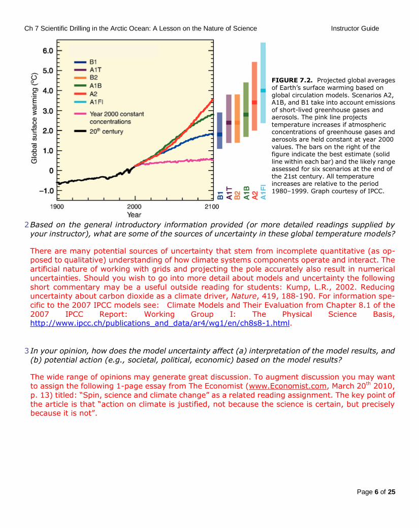
Figures 7.2 and 7.3 (below) show temperature projections based on GCM simulations, reported in
the Intergovernmental Panel on Climate Change (IPCC) 2007 Report (http://www.ipcc.ch/).
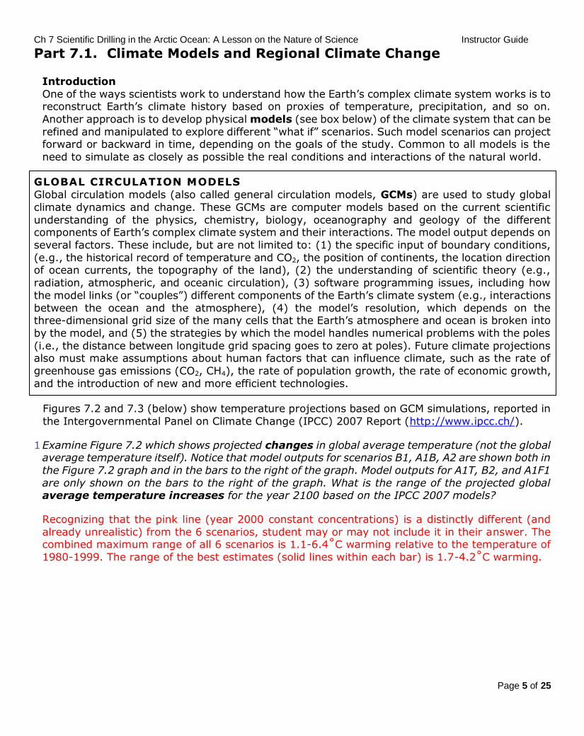
1 Examine Figure 7.2 which shows projected changes in global average temperature (not the global average temperature itself). Notice that model outputs for scenarios B1, A1B, A2 are shown both in
the Figure 7.2 graph and in the bars to the right of the graph. Model outputs for A1T, B2, and A1F1
are only shown on the bars to the right of the graph. What is the range of the projected global average temperature increases for the year 2100 based on the IPCC 2007 models?
Recognizing that the pink line (year 2000 constant concentrations) is a distinctly different (and
already unrealistic) from the 6 scenarios, student may or may not include it in their answer. The combined maximum range of all 6 scenarios is 1.1-6.4˚C warming relative to the temperature of
1980-1999. The range of the best estimates (solid lines within each bar) is 1.7-4.2˚C warming.
Ch 7 Scientific Drilling in the Arctic Ocean: A Lesson on the Nature of Science Instructor Guide
Page 6 of 25
FIGURE 7.2. Projected global averages of Earth’s surface warming based on global circulation models. Scenarios A2, A1B, and B1 take into account emissions of short-lived greenhouse gases and aerosols. The pink line projects temperature increases if atmospheric concentrations of greenhouse gases and aerosols are held constant at year 2000 values. The bars on the right of the figure indicate the best estimate (solid line within each bar) and the likely range assessed for six scenarios at the end of the 21st century. All temperature increases are relative to the period 1980–1999. Graph courtesy of IPCC.
2 Based on the general introductory information provided (or more detailed readings supplied by
your instructor), what are some of the sources of uncertainty in these global temperature models?
There are many potential sources of uncertainty that stem from incomplete quantitative (as op-posed to qualitative) understanding of how climate systems components operate and interact. The
artificial nature of working with grids and projecting the pole accurately also result in numerical
uncertainties. Should you wish to go into more detail about models and uncertainty the following
short commentary may be a useful outside reading for students: Kump, L.R., 2002. Reducing uncertainty about carbon dioxide as a climate driver, Nature, 419, 188-190. For information spe-
cific to the 2007 IPCC models see: Climate Models and Their Evaluation from Chapter 8.1 of the
2007 IPCC Report: Working Group I: The Physical Science Basis, http://www.ipcc.ch/publications_and_data/ar4/wg1/en/ch8s8-1.html.
3 In your opinion, how does the model uncertainty affect (a) interpretation of the model results, and
(b) potential action (e.g., societal, political, economic) based on the model results?
The wide range of opinions may generate great discussion. To augment discussion you may want
to assign the following 1-page essay from The Economist (www.Economist.com, March 20th 2010,
p. 13) titled: “Spin, science and climate change” as a related reading assignment. The key point of
the article is that “action on climate is justified, not because the science is certain, but precisely because it is not”.
Ch 7 Scientific Drilling in the Arctic Ocean: A Lesson on the Nature of Science Instructor Guide
Page 7 of 25
4 Based on the information in the preceding box about GCMs, what are some ways that model
uncertainty could be reduced?
Responses will likely depend on what students identified as sources of uncertainty in question 2. As
pointed out by Kump (2002, Reducing uncertainty about carbon dioxide as a climate driver, Nature
419, 188-190), model uncertainty can be reduced by evaluating models against modern obser-
vation and the best geologic records of warm and cold climates of the past. It is important to test models at the component-level (e.g., is the ocean circulation modeled accurately?) and the sys-
tem-level (the ocean-atmosphere interaction modeled accurately?). See the IPCC link in question
2 for a discussion on model evaluation approaches.
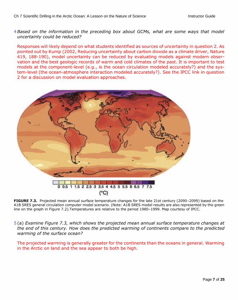
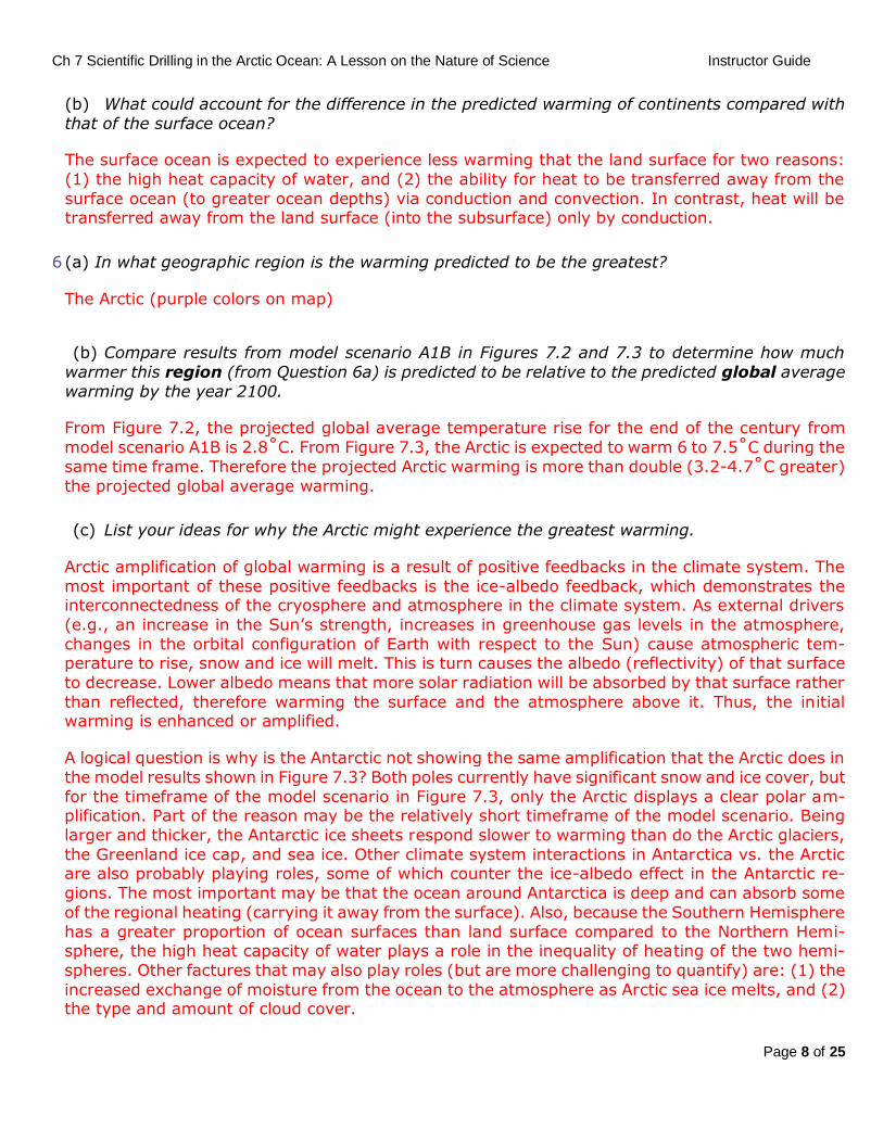
FIGURE 7.3. Projected mean annual surface temperature changes for the late 21st century (2090–2099) based on the A1B SRES general circulation computer model scenario. (Note: A1B SRES model results are also represented by the green line on the graph in Figure 7.2).Temperatures are relative to the period 1980–1999. Map courtesy of IPCC.
5 (a) Examine Figure 7.3, which shows the projected mean annual surface temperature changes at
the end of this century. How does the predicted warming of continents compare to the predicted
warming of the surface ocean?
The projected warming is generally greater for the continents than the oceans in general. Warming
in the Arctic on land and the sea appear to both be high.
Ch 7 Scientific Drilling in the Arctic Ocean: A Lesson on the Nature of Science Instructor Guide
Page 8 of 25
(b) What could account for the difference in the predicted warming of continents compared with
that of the surface ocean?
The surface ocean is expected to experience less warming that the land surface for two reasons:
(1) the high heat capacity of water, and (2) the ability for heat to be transferred away from the
surface ocean (to greater ocean depths) via conduction and convection. In contrast, heat will be transferred away from the land surface (into the subsurface) only by conduction.
6 (a) In what geographic region is the warming predicted to be the greatest?
The Arctic (purple colors on map)
(b) Compare results from model scenario A1B in Figures 7.2 and 7.3 to determine how much
warmer this region (from Question 6a) is predicted to be relative to the predicted global average
warming by the year 2100.
From Figure 7.2, the projected global average temperature rise for the end of the century from
model scenario A1B is 2.8˚C. From Figure 7.3, the Arctic is expected to warm 6 to 7.5˚C during the
same time frame. Therefore the projected Arctic warming is more than double (3.2-4.7˚C greater)
the projected global average warming.
(c) List your ideas for why the Arctic might experience the greatest warming.
Arctic amplification of global warming is a result of positive feedbacks in the climate system. The
most important of these positive feedbacks is the ice-albedo feedback, which demonstrates the interconnectedness of the cryosphere and atmosphere in the climate system. As external drivers
(e.g., an increase in the Sun’s strength, increases in greenhouse gas levels in the atmosphere,
changes in the orbital configuration of Earth with respect to the Sun) cause atmospheric tem-perature to rise, snow and ice will melt. This is turn causes the albedo (reflectivity) of that surface
to decrease. Lower albedo means that more solar radiation will be absorbed by that surface rather
than reflected, therefore warming the surface and the atmosphere above it. Thus, the initial warming is enhanced or amplified.
A logical question is why is the Antarctic not showing the same amplification that the Arctic does in
the model results shown in Figure 7.3? Both poles currently have significant snow and ice cover, but
for the timeframe of the model scenario in Figure 7.3, only the Arctic displays a clear polar am-plification. Part of the reason may be the relatively short timeframe of the model scenario. Being
larger and thicker, the Antarctic ice sheets respond slower to warming than do the Arctic glaciers,
the Greenland ice cap, and sea ice. Other climate system interactions in Antarctica vs. the Arctic are also probably playing roles, some of which counter the ice-albedo effect in the Antarctic re-
gions. The most important may be that the ocean around Antarctica is deep and can absorb some
of the regional heating (carrying it away from the surface). Also, because the Southern Hemisphere
has a greater proportion of ocean surfaces than land surface compared to the Northern Hemi-sphere, the high heat capacity of water plays a role in the inequality of heating of the two hemi-
spheres. Other factures that may also play roles (but are more challenging to quantify) are: (1) the
increased exchange of moisture from the ocean to the atmosphere as Arctic sea ice melts, and (2) the type and amount of cloud cover.
Ch 7 Scientific Drilling in the Arctic Ocean: A Lesson on the Nature of Science Instructor Guide
Page 9 of 25
7 Do these model results provide any scientific motivation to investigate the history of climate change in the Arctic? Explain.
Some students might say no because the model is projecting future climate change not past,
however it is important to understand that models must be tested against modern observations
and records of past change to refine boundary conditions, component parameters, and system interactions. By studying records of past Arctic climate change scientists can investigate regional
vs. global aspects of changing climates, better understand climate system feedbacks, and if age
control is sufficient, explore lead-lag relationships that may play a role not only in past climate change, but future climate change as well.
Part 7.2. Arctic Drilling Challenges and Solutions
1 Make a list of what you think might be unique challenges to drilling into the seafloor in the Arctic
Ocean to recover sediment/rock cores.
Keeping on station to drill (staying on a site for days at a time) is very difficult when sea ice is
constantly moving with the currents. The cold temperatures can make the mechanics of drilling
difficult as well. Being in a remote location makes any re-supply or emergency help difficult.
2 How might these challenges be overcome?
Students may offer hypotheses here that include drilling in the summer months, using special
equipment that is operational in extreme cold temperatures, bringing extra food and medical
supplies, and employing ice-breaker technology.
Drilling only in the summer months is a strategy to maximize the field time during conditions of
warmer weather, longer day-light hours and limited sea ice extent. Even so, staying on site there
can be a challenge and icebreakers are necessary in many locations.
3 Watch a 5 minute movie on the technical approach to drilling in the Arctic by going to:
http://recordings.wun.ac.uk/conf/nwo/oceandrilling2006 then selecting the movie “Drilling the
Arctic”. How was the challenge of staying on-site (or “station”) long enough to drill a deep core
solved?
This was met by having two icebreakers accompany the drill ship during a late summer expedition.
Their job was to break up the sea ice into small enough bits so that the drill ship could stay on
station and drill.
Additional details: The scientific and logistic arguments were compelling and the Arctic Coring
Expedition (ACEX for short) was approved and funded by the Integrated Ocean Drilling Program, an
international consortium of marine research institutions and universities. The expedition took place from August 7 to September 15, 2004. The drill ship, the Vidar Viking, was accompanied by two
ice-breakers, the Oden and Sovetskiy Soyuz. A 428-m–long composite sedimentary section was
constructed by combining cores recovered from 4 holes located <15 km apart along a single
seismic line (Fig. 7.5). The cores were transported to the IODP Core Repository in Bremen, Germany where the scientific team reconvened in November 2004 to split, describe, and sampled
the cores.
Ch 7 Scientific Drilling in the Arctic Ocean: A Lesson on the Nature of Science Instructor Guide
Page 10 of 25
Part 7.3. Need for Scientific Drilling
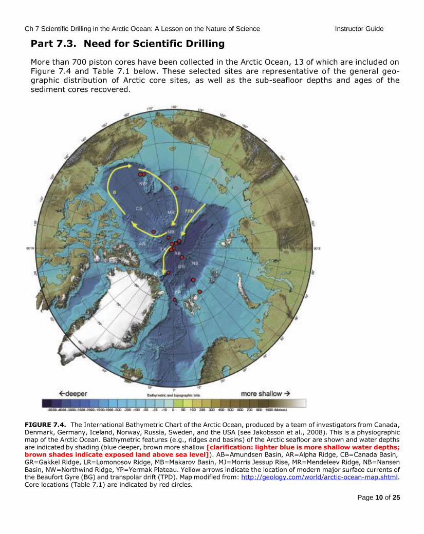
More than 700 piston cores have been collected in the Arctic Ocean, 13 of which are included on
Figure 7.4 and Table 7.1 below. These selected sites are representative of the general geo-graphic distribution of Arctic core sites, as well as the sub-seafloor depths and ages of the
sediment cores recovered.
FIGURE 7.4. The International Bathymetric Chart of the Arctic Ocean, produced by a team of investigators from Canada, Denmark, Germany, Iceland, Norway, Russia, Sweden, and the USA (see Jakobsson et al., 2008). This is a physiographic map of the Arctic Ocean. Bathymetric features (e.g., ridges and basins) of the Arctic seafloor are shown and water depths are indicated by shading (blue deeper, brown more shallow [clarification: lighter blue is more shallow water depths; brown shades indicate exposed land above sea level]). AB=Amundsen Basin, AR=Alpha Ridge, CB=Canada Basin, GR=Gakkel Ridge, LR=Lomonosov Ridge, MB=Makarov Basin, MJ=Morris Jessup Rise, MR=Mendeleev Ridge, NB=Nansen Basin, NW=Northwind Ridge, YP=Yermak Plateau. Yellow arrows indicate the location of modern major surface currents of the Beaufort Gyre (BG) and transpolar drift (TPD). Map modified from: http://geology.com/world/arctic-ocean-map.shtml. Core locations (Table 7.1) are indicated by red circles.
Ch 7 Scientific Drilling in the Arctic Ocean: A Lesson on the Nature of Science Instructor Guide
Page 11 of 25
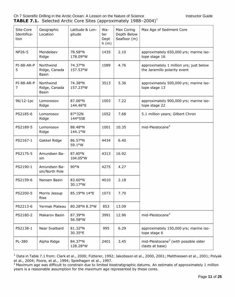
TABLE 7.1. Selected Arctic Core Sites (approximately 1988–2004)1
Site-Core
Identifica-
tion
Geographic
Location
Latitude & Lon-
gitude
Wa-
ter
Dept
h (m)
Max Coring
Depth Below
Seafloor (m)
Max Age of Sediment Core
NP26-5 Mendeleev
Ridge
78.58°N
178.09°W
1435 2.10 approximately 650,000 yrs; marine iso-
tope stage 16
PI-88-AR-P
5
Northwind
Ridge, Canada
Basin
74.37°N
157.53°W
1089 4.76 approximately 1 million yrs; just below
the Jaramillo polarity event
PI-88-AR-P
7
Northwind
Ridge, Canada
Basin
74.38°N
157.23°W
3513 5.36 approximately 500,000 yrs; marine iso-
tope stage 13
96/12-1pc Lomonosov
Ridge
87.06°N
144.46°E
1003 7.22 approximately 900,000 yrs; marine iso-
tope stage 22
PS2185-6 Lomonosov
Ridge
87°32N
144°55E
1052 7.68 5.1 million years; Gilbert Chron
PS2189-5 Lomonosov
Ridge
88.48°N
144.1°W
1001 10.35 mid-Pleistocene2
PS2167-1 Gakkel Ridge 86.57°N
59.1°W
4434 6.40
PS2175-5 Amundsen Ba-
sin
87.40°N
104.05°W
4313 16.92
PS2190-1 Amundsen Ba-
sin/North Pole
90°N 4275 4.27
PS2159-6 Nansen Basin 83.60°N
30.17°W
4010 2.18
PS2200-5 Morris Jessup
Rise
85.19°N 14°E 1073 7.70
PS2213-6 Yermak Plateau 80.28°N 8.3°W 853 13.09
PS2180-2 Makarov Basin 87.39°N
56.58°W
3991 12.96 mid-Pleistocene2
PS2138-1 Near Svalbard 81.32°N
30.35°E
995 6.29 approximately 150,000 yrs; marine iso-
tope stage 6
PL-380 Alpha Ridge 84.37°N
128.28°W
2401 3.45 mid-Pleistocene2 (with possible older
clasts at base)
1 Data in Table 7.1 from: Clark et al., 2000; Fütterer, 1992; Jakobsson et al., 2000, 2001; Matthiessen et al., 2001; Polyak
et al., 2004; Poore, et al., 1994; Spielhagen et al., 1997. 2 Maximum age was difficult to constrain due to limited biostratigraphic datums. An estimate of approximately 1 million years is a reasonable assumption for the maximum age represented by these cores.
Ch 7 Scientific Drilling in the Arctic Ocean: A Lesson on the Nature of Science Instructor Guide
Page 12 of 25
1 From the data shown in Table 7.1 and Figure 7.4, describe the distribution of the coring lo-
cations in terms of geography, water depth, and age, by answering (a)–(c) below.
A reminder that these are only a few of the 700+ piston cores taken in the Arctic, but their locations
represent the coring in the deep basin. It does not represent the coring on the wide continental
shelves, however.
There is a nice online resource describing what piston cores are at: http://oceanworld.tamu.edu/students/forams/forams_piston_coring.htm.
(a) Are cores mostly on bathymetric highs, mostly in basins, or distributed between these two settings?
The coring tends to focus on bathymetric highs, but there are certainly exceptions. Given the
challenging weather and sea ice conditions in the Arctic it is easy to see why piston coring in the deep basin is less common (more time on station).
(b) What is the maximum sub-seafloor depth reached by these cores?
Max sub-seafloor depth is 16.92 mbsf from a core in the Amundsen basin.
(c) What is the maximum age of the sediment in these cores?
Many of these cores don’t have an absolute age, but are listed only with relative ages. [It is difficult
to date sediments from the Arctic – the preservation of calcareous microfossils is very poor, the
abundance of other types of organic-walled (dinocysts) or siliceous microfossils (diatoms) may be diluted/maske, by terrigenous sediments, making age determination more challenging]. So
mid-Pleistocene is the maximum age (about 1 million years old), although some older clasts may
have been recovered on Alpha Ridge. The age of these is uncertain.
2 Use data in Table 7.1 to calculate the percentage of Cenozoic time that the sediment records
of these Arctic cores represents. Note the Cenozoic Era includes the last 65.5 million years. Show
your work.
Using 1,000,000 yr BP as the oldest age of sediment from the chart (which also represents a mid-Pleistocene age) then:
(1,000,000 yrs / 66,500,000 yrs) * 100 = 1.5% of Cenozoic time that the Arctic cores have
penetrated.
Ch 7 Scientific Drilling in the Arctic Ocean: A Lesson on the Nature of Science Instructor Guide
Page 13 of 25
3 Based on what you have learned in this exercise so far, do you think that the Cenozoic geologic
history (including climate history) of the Arctic Ocean was well understood from the sediments recovered by piston cores? Explain.
Not well at all for anything older than the mid-Pleistocene - it is a black hole so to speak. However,
the mid-Pleistocene and younger geologic history should be reasonably well reconstructed based
on both the 700 + cores, and inferred from nearby terrestrial records.
One way to make this point is to ask student to draw a line along the vertical axis of Figure 7.6 at
the end of Part 7.3 (this figure which summarizes Cenozoic geologic history) showing the geologic
time intervals that Arctic coring has recovered. This line will be short - only from today (0) to the mid-Pleistocene (~1 Ma, given the scale.) The Arctic cores couldn’t have contributed much data on
this topic, except for good regional coverage for the Pleistocene-Holocene; really nothing on the
transition time from greenhouse to icehouse (think back to Chapter 5). The paradigm of under-standing about Cenozoic climate change from a Greenhouse to an Icehouse World lacks any
long-term data sets from the Arctic Ocean, the Northern Hemisphere’s polar region. Rather, it is
long cores from the sub-Arctic that have defined the onset of ice growth for the Northern Hemi-
sphere.
INTEGRATED OCEAN DRILLING PROGRAM ARCTIC CORING EXPEDITION (ACEX)
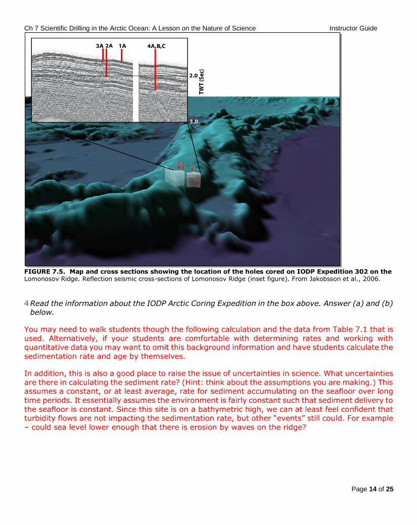
In 2004 a team of scientists and technicians drilled five holes within 16 km of each other along the crest of the Lomonosov Ridge (Figure 7.5) in the central Arctic Ocean. The holes were distributed
between 87°N and 88°N in water depths between 1100 m and 1200 m and were all in international
waters. Some of the pieces of information that helped the science team select these particular lo-
cations were seismic reflection profiles (see Figure 7.5 inset; like “sonograms” of the subsurface seafloor) from seismic survey cruises that suggested the sedimentary sequence along this part of the
ridge was very thick. It was estimated that there were 450 m of sediments overlying the harder
basement rock in this area.
It was predicted that this 450 m sedimentary sequence represented about 56 million years of
history. This estimate is based on the previously known sedimentation rate on the Lomonosov Ridge of 7.22 m/0.9 myr=8 m/myr (calculated from Table 7.1) and assumes a constant sedimentation rate
for the entire 450 m thickness of sediment inferred from the seismic profile.
Ch 7 Scientific Drilling in the Arctic Ocean: A Lesson on the Nature of Science Instructor Guide
Page 14 of 25
FIGURE 7.5. Map and cross sections showing the location of the holes cored on IODP Expedition 302 on the Lomonosov Ridge. Reflection seismic cross-sections of Lomonosov Ridge (inset figure). From Jakobsson et al., 2006.
4 Read the information about the IODP Arctic Coring Expedition in the box above. Answer (a) and (b) below.
You may need to walk students though the following calculation and the data from Table 7.1 that is
used. Alternatively, if your students are comfortable with determining rates and working with quantitative data you may want to omit this background information and have students calculate the
sedimentation rate and age by themselves.
In addition, this is also a good place to raise the issue of uncertainties in science. What uncertainties
are there in calculating the sediment rate? (Hint: think about the assumptions you are making.) This assumes a constant, or at least average, rate for sediment accumulating on the seafloor over long
time periods. It essentially assumes the environment is fairly constant such that sediment delivery to
the seafloor is constant. Since this site is on a bathymetric high, we can at least feel confident that turbidity flows are not impacting the sedimentation rate, but other “events” still could. For example
– could sea level lower enough that there is erosion by waves on the ridge?
Ch 7 Scientific Drilling in the Arctic Ocean: A Lesson on the Nature of Science Instructor Guide
Page 15 of 25
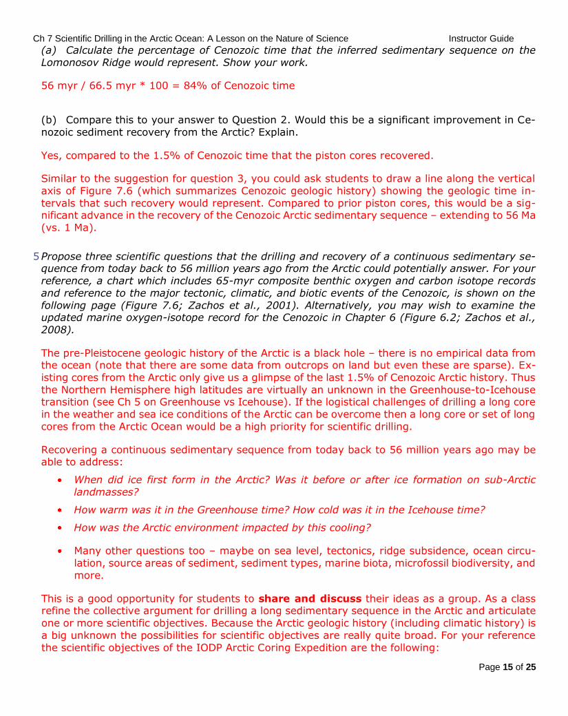
(a) Calculate the percentage of Cenozoic time that the inferred sedimentary sequence on the
Lomonosov Ridge would represent. Show your work.
56 myr / 66.5 myr * 100 = 84% of Cenozoic time
(b) Compare this to your answer to Question 2. Would this be a significant improvement in Ce-
nozoic sediment recovery from the Arctic? Explain.
Yes, compared to the 1.5% of Cenozoic time that the piston cores recovered.
Similar to the suggestion for question 3, you could ask students to draw a line along the vertical
axis of Figure 7.6 (which summarizes Cenozoic geologic history) showing the geologic time in-
tervals that such recovery would represent. Compared to prior piston cores, this would be a sig-nificant advance in the recovery of the Cenozoic Arctic sedimentary sequence – extending to 56 Ma
(vs. 1 Ma).
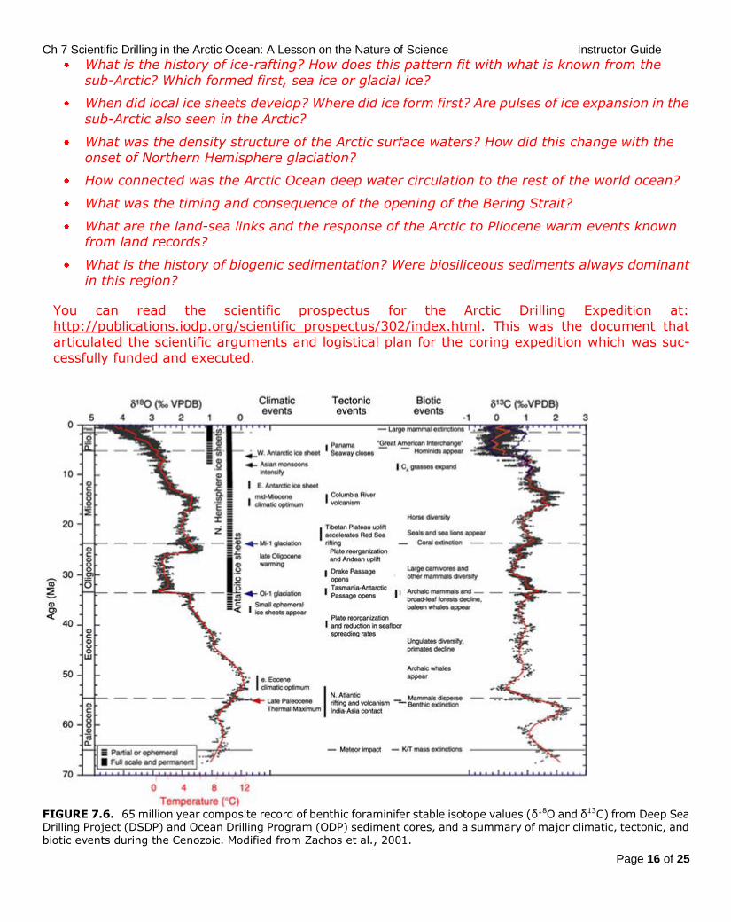
5 Propose three scientific questions that the drilling and recovery of a continuous sedimentary se-quence from today back to 56 million years ago from the Arctic could potentially answer. For your
reference, a chart which includes 65-myr composite benthic oxygen and carbon isotope records
and reference to the major tectonic, climatic, and biotic events of the Cenozoic, is shown on the
following page (Figure 7.6; Zachos et al., 2001). Alternatively, you may wish to examine the updated marine oxygen-isotope record for the Cenozoic in Chapter 6 (Figure 6.2; Zachos et al.,
2008).
The pre-Pleistocene geologic history of the Arctic is a black hole – there is no empirical data from the ocean (note that there are some data from outcrops on land but even these are sparse). Ex-
isting cores from the Arctic only give us a glimpse of the last 1.5% of Cenozoic Arctic history. Thus
the Northern Hemisphere high latitudes are virtually an unknown in the Greenhouse-to-Icehouse transition (see Ch 5 on Greenhouse vs Icehouse). If the logistical challenges of drilling a long core
in the weather and sea ice conditions of the Arctic can be overcome then a long core or set of long
cores from the Arctic Ocean would be a high priority for scientific drilling.
Recovering a continuous sedimentary sequence from today back to 56 million years ago may be able to address:
When did ice first form in the Arctic? Was it before or after ice formation on sub-Arctic
landmasses?
How warm was it in the Greenhouse time? How cold was it in the Icehouse time?
How was the Arctic environment impacted by this cooling?
Many other questions too – maybe on sea level, tectonics, ridge subsidence, ocean circu-
lation, source areas of sediment, sediment types, marine biota, microfossil biodiversity, and
more.
This is a good opportunity for students to share and discuss their ideas as a group. As a class refine the collective argument for drilling a long sedimentary sequence in the Arctic and articulate
one or more scientific objectives. Because the Arctic geologic history (including climatic history) is
a big unknown the possibilities for scientific objectives are really quite broad. For your reference
the scientific objectives of the IODP Arctic Coring Expedition are the following:
Ch 7 Scientific Drilling in the Arctic Ocean: A Lesson on the Nature of Science Instructor Guide
Page 16 of 25
What is the history of ice-rafting? How does this pattern fit with what is known from the
sub-Arctic? Which formed first, sea ice or glacial ice?
When did local ice sheets develop? Where did ice form first? Are pulses of ice expansion in the
sub-Arctic also seen in the Arctic?
What was the density structure of the Arctic surface waters? How did this change with the
onset of Northern Hemisphere glaciation?
How connected was the Arctic Ocean deep water circulation to the rest of the world ocean?
What was the timing and consequence of the opening of the Bering Strait?
What are the land-sea links and the response of the Arctic to Pliocene warm events known from land records?
What is the history of biogenic sedimentation? Were biosiliceous sediments always dominant
in this region?
You can read the scientific prospectus for the Arctic Drilling Expedition at:
http://publications.iodp.org/scientific_prospectus/302/index.html. This was the document that
articulated the scientific arguments and logistical plan for the coring expedition which was suc-
cessfully funded and executed.
FIGURE 7.6. 65 million year composite record of benthic foraminifer stable isotope values (δ18O and δ13C) from Deep Sea Drilling Project (DSDP) and Ocean Drilling Program (ODP) sediment cores, and a summary of major climatic, tectonic, and biotic events during the Cenozoic. Modified from Zachos et al., 2001.
Ch 7 Scientific Drilling in the Arctic Ocean: A Lesson on the Nature of Science Instructor Guide
Page 17 of 25
Part 7.4. Results of the Arctic Drilling Expedition
The Arctic Coring Expedition (ACEX; IODP Expedition 302) was considered “transformative” in the more than 40 year history of scientific ocean drilling, because of both the logistical challenges it
overcame to recover a long sedimentary sequence from the central Arctic Ocean and the scientific
results that had an impact on our perceptions of Cenozoic climate. Some of these scientific results
are embedded in other chapters of this book (see Chapter 8, Figure 8.4; Chapter 9, Figures 9.20 & 9.21; Chapter 14, Figures 14.6 & 14.7). In this investigation, you will read a synthesis paper on the
Arctic Coring Expedition to identify some of the key findings.
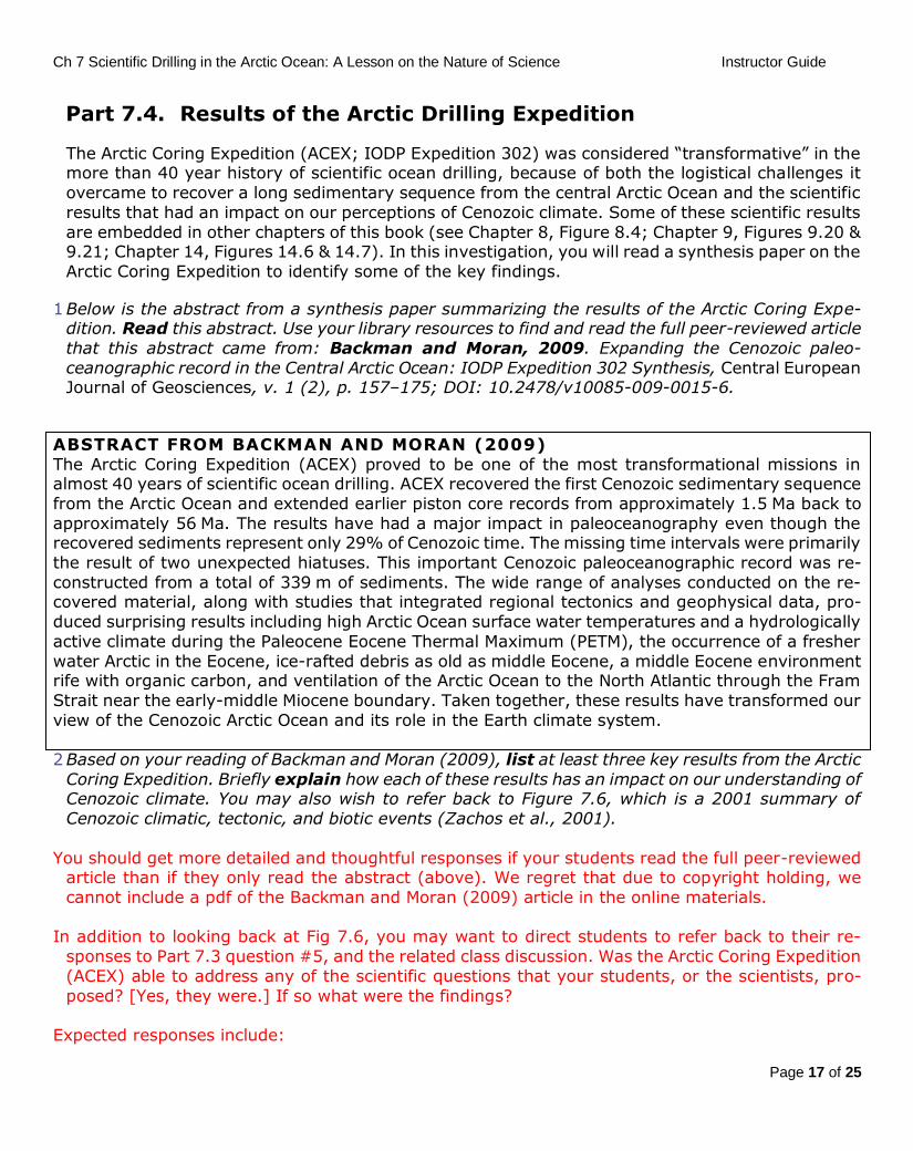
1 Below is the abstract from a synthesis paper summarizing the results of the Arctic Coring Expe-dition. Read this abstract. Use your library resources to find and read the full peer-reviewed article
that this abstract came from: Backman and Moran, 2009. Expanding the Cenozoic paleo-
ceanographic record in the Central Arctic Ocean: IODP Expedition 302 Synthesis, Central European Journal of Geosciences, v. 1 (2), p. 157–175; DOI: 10.2478/v10085-009-0015-6.
ABSTRACT FROM BACKMAN AND MORAN (2009)
The Arctic Coring Expedition (ACEX) proved to be one of the most transformational missions in almost 40 years of scientific ocean drilling. ACEX recovered the first Cenozoic sedimentary sequence
from the Arctic Ocean and extended earlier piston core records from approximately 1.5 Ma back to
approximately 56 Ma. The results have had a major impact in paleoceanography even though the recovered sediments represent only 29% of Cenozoic time. The missing time intervals were primarily
the result of two unexpected hiatuses. This important Cenozoic paleoceanographic record was re-
constructed from a total of 339 m of sediments. The wide range of analyses conducted on the re-covered material, along with studies that integrated regional tectonics and geophysical data, pro-
duced surprising results including high Arctic Ocean surface water temperatures and a hydrologically
active climate during the Paleocene Eocene Thermal Maximum (PETM), the occurrence of a fresher
water Arctic in the Eocene, ice-rafted debris as old as middle Eocene, a middle Eocene environment rife with organic carbon, and ventilation of the Arctic Ocean to the North Atlantic through the Fram
Strait near the early-middle Miocene boundary. Taken together, these results have transformed our
view of the Cenozoic Arctic Ocean and its role in the Earth climate system.
2 Based on your reading of Backman and Moran (2009), list at least three key results from the Arctic
Coring Expedition. Briefly explain how each of these results has an impact on our understanding of Cenozoic climate. You may also wish to refer back to Figure 7.6, which is a 2001 summary of
Cenozoic climatic, tectonic, and biotic events (Zachos et al., 2001).
You should get more detailed and thoughtful responses if your students read the full peer-reviewed article than if they only read the abstract (above). We regret that due to copyright holding, we
cannot include a pdf of the Backman and Moran (2009) article in the online materials.
In addition to looking back at Fig 7.6, you may want to direct students to refer back to their re-
sponses to Part 7.3 question #5, and the related class discussion. Was the Arctic Coring Expedition
(ACEX) able to address any of the scientific questions that your students, or the scientists, pro-
posed? [Yes, they were.] If so what were the findings?
Expected responses include:
Ch 7 Scientific Drilling in the Arctic Ocean: A Lesson on the Nature of Science Instructor Guide
Page 18 of 25
The surprising low recovery of the sediments – while the coring extended though the Cenozoic
sequence, the recovery of the cores was proving challenging largely due (a) drilling operations
issues and (b) to two major hiatuses [this is explored more in questions 4-6. Therefore the record while long, is not as continuous as expected – recovered sediments represented only
29% of Cenozoic time. Even with this lower than expected recovery, the record provided
amazing insight into Cenozoic Arctic climate evolution (see points below). A very warm and wet (high precipitation) Arctic during the PETM (55 Ma). The greenhouse
world was even warmer (warmed 5-6◦C from 18◦C to over 23◦C summer temps) than expected
in the Arctic. High terrigenous sedimentation rates suggest a very active hydrologic cycle. This
is the exact opposite condition that the Arcitc experiences today (cold and dry). These results have implications for projections of global warming and regional responses in the future.
The Arctic was much fresher (very low salinity) during the Eocene. The arctic was at least
seasonally stratified, with a fresh water lens (abundant fresh water fern fossils support this);
some suggest the Black Sea is a modern analogue for the Eocene Arctic. The Arctic had high biologic productivity in the Eocene, producing a lot of organic carbon,
which has accumulated [not been oxidized] because of the early Cenozoic low oxygen con-
dition (deep waters were poorly ventilated) in the deeper waters. This raised interest for
potential hydrocarbon (resource) exploration, but the carbon is likely to a too immature stage
(not yet oil and gas). Ice-rafting starting in the middle Eocene (~46 Ma). This suggests the climatic transition from
Greenhouse to Icehouse conditions in the Arctic started much earlier than previously thought,
with sea ice likely forming before glaciers, but well before widespread Northern Hemisphere
ice sheets (~2.7 Ma; see Ch 14). The Arctic was fairly isolated from the global ocean system until the Fram Strait opened
(tectonic opening) in the early-middle Miocene. This ventilation may have inhibited deep
water formation in the North Atlantic because of the influx of fresh Arctic waters to the At-
lantic. There may be tectonic results that are brought up too if the student read the paper and not
just the abstract. Essentially the ACEX record supports the interpretation that the Lomonosov
Ridge is a continental sliver of the Eurasian margin (former continental shelf), which rifted in
the late Paleocene, and was tectonically isolated from the margin by middle Eocene. In ad-dition, there is an unusual subsidence history. The ridge likely remained at epipelagic depths
(0-200m) until the early Miocene, and then subsequently subsided to its current depth of ~
1250 mbsf.
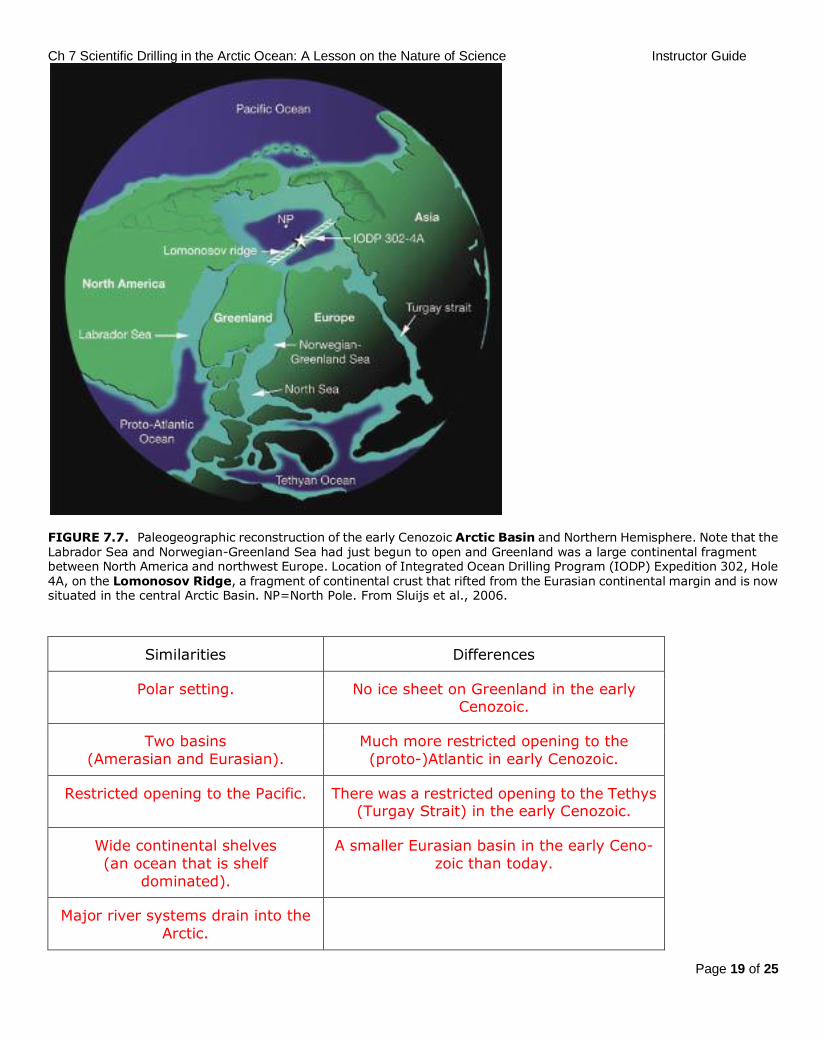
3 The reconstructed paleogeographic setting of the Arctic Ocean in the early Cenozoic (Figure 7.7)
shares some similarities with the geography of the Arctic Ocean today (Figure 7.4), but also in-
cludes some important differences. List two similarities and two differences between the paleo-
geographic settings of the Arctic in the Early Cenozoic compared to today.
See expected responses in the table on following page
Ch 7 Scientific Drilling in the Arctic Ocean: A Lesson on the Nature of Science Instructor Guide
Page 19 of 25
FIGURE 7.7. Paleogeographic reconstruction of the early Cenozoic Arctic Basin and Northern Hemisphere. Note that the Labrador Sea and Norwegian-Greenland Sea had just begun to open and Greenland was a large continental fragment between North America and northwest Europe. Location of Integrated Ocean Drilling Program (IODP) Expedition 302, Hole 4A, on the Lomonosov Ridge, a fragment of continental crust that rifted from the Eurasian continental margin and is now situated in the central Arctic Basin. NP=North Pole. From Sluijs et al., 2006.
Similarities Differences
Polar setting. No ice sheet on Greenland in the early Cenozoic.
Two basins
(Amerasian and Eurasian).
Much more restricted opening to the
(proto-)Atlantic in early Cenozoic.
Restricted opening to the Pacific. There was a restricted opening to the Tethys (Turgay Strait) in the early Cenozoic.
Wide continental shelves
(an ocean that is shelf
dominated).
A smaller Eurasian basin in the early Ceno-
zoic than today.
Major river systems drain into the
Arctic.
Ch 7 Scientific Drilling in the Arctic Ocean: A Lesson on the Nature of Science Instructor Guide
Page 20 of 25
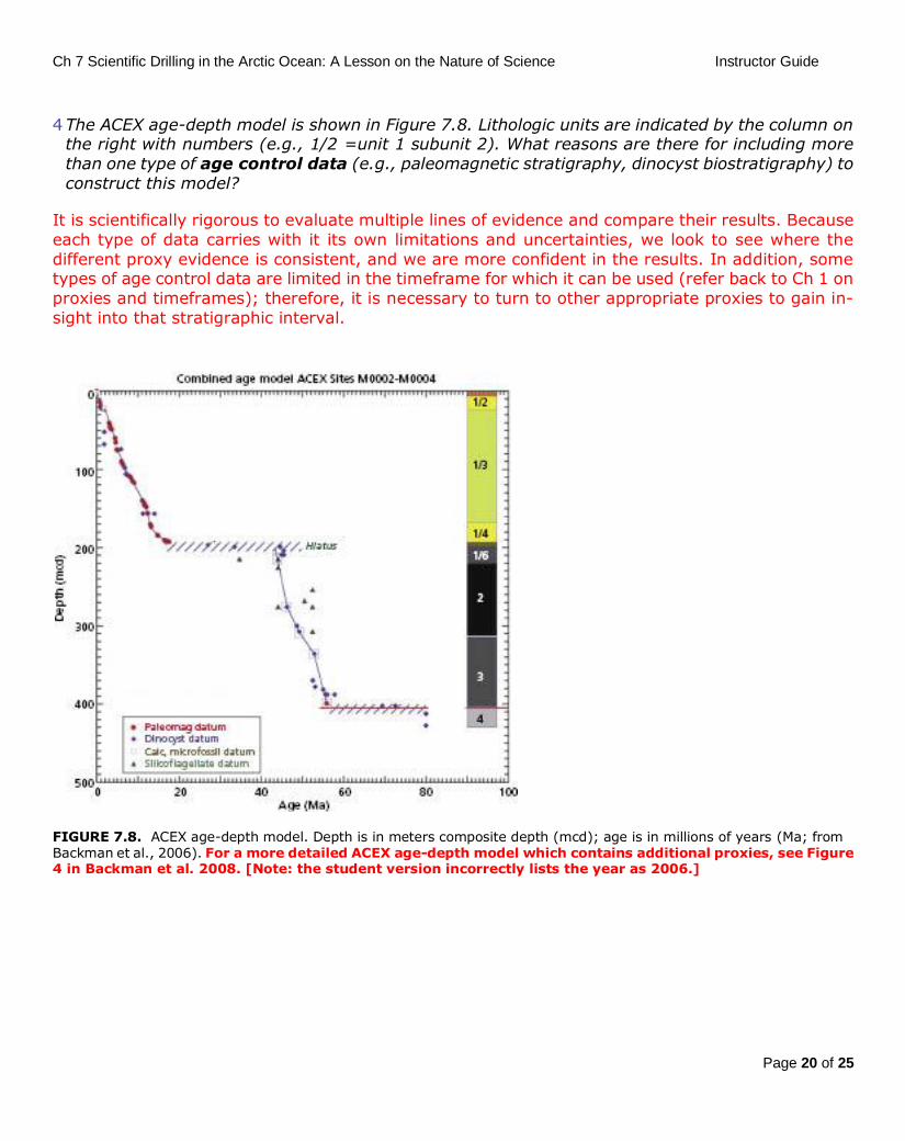
4 The ACEX age-depth model is shown in Figure 7.8. Lithologic units are indicated by the column on the right with numbers (e.g., 1/2 =unit 1 subunit 2). What reasons are there for including more
than one type of age control data (e.g., paleomagnetic stratigraphy, dinocyst biostratigraphy) to
construct this model?
It is scientifically rigorous to evaluate multiple lines of evidence and compare their results. Because
each type of data carries with it its own limitations and uncertainties, we look to see where the
different proxy evidence is consistent, and we are more confident in the results. In addition, some types of age control data are limited in the timeframe for which it can be used (refer back to Ch 1 on
proxies and timeframes); therefore, it is necessary to turn to other appropriate proxies to gain in-
sight into that stratigraphic interval.
FIGURE 7.8. ACEX age-depth model. Depth is in meters composite depth (mcd); age is in millions of years (Ma; from Backman et al., 2006). For a more detailed ACEX age-depth model which contains additional proxies, see Figure 4 in Backman et al. 2008. [Note: the student version incorrectly lists the year as 2006.]
Ch 7 Scientific Drilling in the Arctic Ocean: A Lesson on the Nature of Science Instructor Guide
Page 21 of 25
5 Calculate the sedimentation rates for (a) lithologic unit 1/3 and (b) lithologic unit 1/4, in meters per
million years (m/myr). Show your work below and label the age model (Figure 7.8) with these two sedimentation rates.
Minor clarification: these are really subunits (1/3 = lithologic unit 1 subunit 3).
The answer may vary a bit since student’s are reading off of the graph (Fig 7.8) rather than being
supplied with a data table. Expected calculations are:
(a) Lithologic unit 1/3 encompasses 0 to 140 mbsf, and 0 to ~12 Ma.
140m/12myr = 11.6 m/myr
Therefore lithologic unit 1/3 linear sedimentation rate of ~ 11.6 m/myr (newer estimates are ~14.5 m/myr; see Backman et al., 2008).
(b) Lithologic unit 1/4 extends from ~150 mbsf to ~195 mvsf, and ~12 to 18 Ma.
45m/6 myr = 7.5 m/myr
Therefore lithologic unit 1/3 has a linear sedimentation rate of ~7.5 m/myr (newer estimates are
8 m/myr; see Backman et al, 2008).
6 A major hiatus occurs within lithologic unit 1/5 (Figure 7.8); this hiatus was unexpected based on
the pre-drilling seismic data (Figure7.5).
(a) Based on the data in Figure 7.7, how much time does the hiatus in unit 1/5 represent?
Based on the age model in Figure 7.8, the hiatus extends from ~44 Ma to 18 Ma. Therefore spans
~26 million years.
(b) How does this hiatus impact the efforts to reconstruct Cenozoic paleoclimates from the ACEX
sedimentary record?
At the most basic level there is a major gap in timeline of reconstruction; therefore it restricts paleoclimatic interpretations to before and after this gap in the sequence, although one can
speculate on what caused this (e.g., was the Lomonosov Ridge above sea level and later eroded by
wave action?). The Antarctic ice sheet experienced rapid and major expansion during the Eo-
cene-Oligocene transition, and it would be very interesting to see learn what was happening in the Arctic at this time, but because of the hiatus in the ACEX record we cannot yet address that.
(c) In the future, how might we obtain a sediment record that spans this “missing” timeframe?
Future coring expeditions that target (using geophysical surveys; see fig 7.5) the stratigraphic interval of interest.
Ch 7 Scientific Drilling in the Arctic Ocean: A Lesson on the Nature of Science Instructor Guide
Page 22 of 25
III. Summative Assessment
There are several ways the instructor can assess student learning after completion of this exercise.
For example, students should be able to answer the following questions after completing this ex-ercise:
1. (a) How do temperature projects for the Arctic differ from the global average temperature projects? (b) What is polar amplification and why does it occur?
2. The science of reconstructing past climates advances best when
a. Mismatched data from geologic archives and model outputs are disregarded or thrown out b. Climate models strive towards using the largest grid box possible
c. The strengths and limitations of both the data derived from geologic archives
and the models are constantly tested against one another d. All of the above
e. B and C only
3. Describe and explain 2 examples of regional variability in the IPCC model-projected temperature
changes for the end of this century.
4. Recovering long sedimentary sequences (of hundreds of meters in length) in the Arctic Ocean requires
a. Minimal technology and therefore has been done for several centuries
b. Drilling in the winter months c. Ice breaker ships to keep the drill ship from being crushed by drifting sea ice
d. Both B and C
5. Drilling in the Arctic is challenging for several reasons, but these challenges have been overcome
because the scientific rationale for drilling in the Arctic is so strong. In a short paragraph provide
an argument for recovering long sedimentary sequences in the Arctic Ocean.
6. Explain in 2-3 sentences how research is enabled by technology, using the Arctic drilling as an
example.
7. If you know length of a sediment core and the average sedimentation rate, how would you de-
termine the maximum sediment age of that core? What assumptions are made in with such a
calculation?
8. (a) Drawing from your work in Parts 7.1-7.3 describe and justify one scientific objective for
recovering a long sedimentary sequence in the Arctic Ocean. (b) Then drawing from your work in
Part 7.4 (including the suggested reading) describe the Arctic Coring Expedition findings that address this objective.
9. Calculate the sedimentation rates for Lithologic Units 2 and 3 (Figure 7.8). [As an instructor you may wish to refer to Backman et al., 2008 for a more detailed age model]
10.Determine the duration of the hiatus marking the Lithologic 3-4 unit boundary (Figure 7.8).
Ch 7 Scientific Drilling in the Arctic Ocean: A Lesson on the Nature of Science Instructor Guide
Page 23 of 25
IV. Supplemental Materials
The Intergovernmental Panel on Climate Change (IPCC) has numerous references online (http://www.ipcc.ch/) for scientists and non-scientists. The 2007 Synthesis Report Summary
for Policymakers is a good place to begin:
http://www.ipcc.ch/publications_and_data/ar4/syr/en/spm.html There are several scientific proposals (e.g., #708, 746, 756) to return to the Arctic for further
seafloor drilling research. All active IODP proposal can be found at:
http://www.iodp.org/active-proposals/
The scientific results of the Arctic Coring Expedition continue to be published. The following are good places to start to learn more about the outcomes of this expedition:
o The European Consortium for Ocean Research Drilling has a 2-page online brochure on
ACEX: http://www.ecord.org/pub/ACEX.pdf o Backman, J., and Moran, K., 2009, Expanding the Cenozoic paleoceanographic record
in the central Arctic Ocean: IODP Expedition 302 synthesis: Central European Journal of
Geoscience, v. 1, p. 157-175, doi:10.2478/v10085-009-0015-6. For a good discussion of the uncertainties in climate science, including models, that is written
at a level for non-specialists see: Kump, L.R., 2002, Reducing uncertainty about carbon di-
oxide as a climate driver: Nature, v. 419, p. 188-190.
For a broad discussion of models see: Oreskes, N., 1998, Why Believe a Computer? Models, Measures, and Meaning in the Natural World, in Schneiderman, J., ed., The Earth Around Us:
Maintaining a Livable Planet, Freeman, New York, Ch. 6, p. 70-82.
For information specific to the 2007 IPCC model evaluation, see: Climate Models and Their Evaluation from Chapter 8.1 of the 2007 IPCC Report: Working Group I: The Physical Science
Basis, http://www.ipcc.ch/publications_and_data/ar4/wg1/en/ch8s8-1.html.
Figure 4 from the following article is especially useful in summarizing model results on polar amplification: Masson-Delmotte et al., 2006, Past and future polar amplification of climate
change: climate model intercomparisons and ice-core constraints: Climate Dynamics, v. 26,
p. 513-529.
The 1-page essay “Spin, science and climate change” in The Economist (www.Economist.com, March 20th 2010, p. 13) thoughtfully addresses the societal and political implications of un-
certainty in climate change research.
A menu of several short videos to download on Drilling Extreme Climates, including the Arctic Coring Expedition: http://recordings.wun.ac.uk/conf/nwo/oceandrilling2006
Download this 5 minute video to explore the process of ocean drilling science - from proposal
ideas all the way to reconstructing Earth's past climate history: http://www.oceanleadership.org/learning/materials/multimedia
To read a paper on the technical challenges and acomplishments of drilling a long core in the
Arctic go to:
http://publications.iodp.org/proceedings/302/EXP_REPT/CHAPTERS/302_106.PDF You can read the scientific prospectus for the Arctic Drilling Expedition at:
http://publications.iodp.org/scientific_prospectus/302/index.html. this was the document
that articulated the scientific arguments and logistical plan for the coring expedition which was successfully funded and executed.
To learn more about piston cores go to:
http://oceanworld.tamu.edu/students/forams/forams_piston_coring.htm
For interactive 2D maps and 3D globes that support Arctic science go to the Arctic Research Mapping Application (ARMAP) site: http://armap.org.
Ch 7 Scientific Drilling in the Arctic Ocean: A Lesson on the Nature of Science Instructor Guide
Page 24 of 25
V. References
Backman, J. and Moran, K., 2009, Expanding the Cenozoic paleoceanographic record in the Central Arctic Ocean: IODP Expedition 302 Synthesis. Central European Journal of Geosciences, 1 (2),
157–75; doi: 10.2478/v10085-009-0015-6.
Backman, J., et al., and Expedition 302 Scientists, 2006, Proceedings of the Integrated Ocean
Drilling Program, vol. 302, College Station, TX, Ocean Drilling Program, doi.10.2204/iodp.proc.302.104.2006.
Backman, J., et al., 2008, Age model and core seismic integration for the Cenozoic ACEX sediments
from the Lomonosov Ridge. Paleoceanography, 23, doi:10.1029/2007PA001476.
Clark, D.L., et al., 2000, Orphan Arctic Ocean metasediment clasts: Local derivation of from Alpha
Ridge or pre-2.6 Ma ice rafting? Geology, 28, 1143–6.
Fütterer, D.K., 1992, ARCTIC’91: The expedition ARK-VIII/3 of R/V Polarstern in 1991. Alfred
Wegener Institute for Polar and Marine Research, Bremerhaven, Germany. Report on Polar Re-search, vol. 107, 267 pp.
Jakobsson, M., et al., 2000, Manganese and color cycles in Arctic Ocean sediments contrain Pleis-
tocene chronology. Geology, 28, 23–6.
Jakobsson, M., et al., 2001, Pleistocene stratigraphy and paleoenvironmental variations from Lo-
monosov Ridge sediments, central Arctic Ocean. Global Planetary Change, 31, 1–22.
Jakobsson, M., Flodén, T., and the Expedition 302 Scientists, 2006. Expedition 302 geophysics: integrating past data with new results,” in Backman, J., Moran, K., McInroy, D.B., et al., Pro-
ceedings of the Integrated Ocean Drilling Program 302 (Edinburgh: Integrated Ocean Drilling
Program Management International, Inc., 2006). doi:10.2204/iodp.proc.302.102.2006.
Jakobsson, M., et al., 2008. An improved bathymetric portrayal of the Arctic Ocean: Implications for ocean modeling and geological, geophysical and oceanographic analyses. Geophysical Research
Letters, 35, L07602, doi:10.1029/2008GL033520
Moran, K., et al., 2006. The Cenozoic palaeoenvironment of the Arctic Ocean. Nature, 441, 601–6.
Matthiessen, J., et al., 2001. Late Quaternary dinoflagellate cyst stratigraphy at the Eurasian con-
tinental margin, Arctic Ocean: indications for Atlantic water inflow in the past 150,000 years. Global
and Planetary Change, 31, 65–86.
Polyak, L., et al., 2004, Contrasting glacial/interglacial regimes in the western Arctic Ocean as
exemplified by a sedimentary record from the Mendeleev Ridge. Palaeogeography, Palaeoclima-
tology, Palaeoecology, 203, 73–93.
Poore, R.Z., et al., 1994, Quaternary stratigraphy and paleoceanography of the Canada Basin, Western Arctic Ocean US. Geological Survey Bulletin, vol. 2080, 34 pp.
Sluijs, A., et al., and the Expedition 302 Scientists, 2006, Subtropical Arctic Ocean temperatures
during the Palaeocene/Eocene thermal maximum. Nature, 441, 610–13.
Spielhagen, R.F., et al., 1997, Arctic Ocean evidence for late Quaternary initiation of northern
Eurasian ice sheet. Geology, 25 (9), 783–6.

Ch 7 Scientific Drilling in the Arctic Ocean: A Lesson on the Nature of Science Instructor Guide
Page 25 of 25
Zachos, J., et al., 2001, Trends, rhythms, and aberrations in global climate 65 Ma to present. Sci-ence, 292, 686–93.
Zachos, J., et al., 2008. An early Cenozoic perspective on greenhouse warming and carbon-cycle
dymanics. Nature, 451, 279–83.