IM 12D7B5-E-E 4th edition

InstructionManual

YOKOGAWA

Model SC450GConductivity / Resistivity Transmitter

Commissioning

PREFACE

Electrostatic dischargeThe EXAxt transmitter contains devices that can be damaged by electrostatic discharge. When servicing this equipment, please observe proper procedures to prevent such damage. Replacement components should be shipped in conductive packaging. Repair work should be done at grounded workstations using grounded soldering irons and wrist straps to avoid electrostatic discharge.

Installation and wiringThe EXAxt transmitter should only be used with equipment that meets the relevant IEC, American or Canadian standards. Yokogawa accepts no responsibility for the misuse of this unit.

The Instrument is packed carefully with shock absorbing materials, nevertheless, the instrument may be damaged or broken if subjected to strong shock, such as if the instrument is dropped. Handle with care.

Do not use an abrasive or organic solvent in cleaning the instrument.

NoticeContents of this manual are subject to change without notice. Yokogawa is not responsible for damage to the instrument, poor performance of the instrument or losses resulting from such, if the problems are caused by:• Incorrect operation by the user.• Use of the instrument in incorrect

applications.• Use of the instrument in an inappropriate

environment or incorrect utility program.• Repair or modification of the related

instrument by an engineer not authorised by Yokogawa.

Warranty and serviceYokogawa products and parts are guaranteed free from defects in workmanship and material under normal use and service for a period of (typically) 12 months from the date of shipment from the manufacturer. Individual sales organisations can deviate from the typical warranty period, and the conditions of sale relating to the original purchase order should be consulted. Damage caused by wear and tear, inadequate maintenance, corrosion, or by the effects of chemical processes are excluded from this warranty coverage.

In the event of warranty claim, the defective goods should be sent (freight paid) to the service department of the relevant sales organisation for repair or replacement (at Yokogawa discretion). The following information must be included in the letter accompanying the returned goods:• Part number, model code and serial number• Original purchase order and date• Length of time in service and a description

of the process• Description of the fault, and the

circumstances of failure• Process/environmental conditions that may

be related to the failure of the device.• A statement whether warranty or non-

warranty service is requested• Complete shipping and billing instructions

for return of material, plus the name and phone number of a contact person who can be reached for further information.

Returned goods that have been in contact with process fluids must be decontaminated/disinfected before shipment. Goods should carry a certificate to this effect, for the health and safety of our employees. Material safety data sheets should also be included for all components of the processes to which the equipment has been exposed.

WARNING

CAUTION

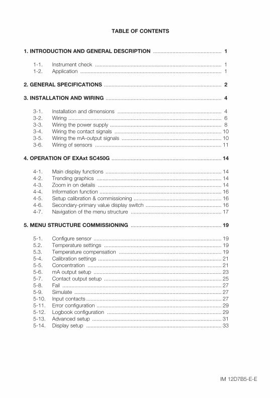
TABLE OF CONTENTS

1. INTRODUCTION AND GENERAL DESCRIPTION .............................................. 1

1-1. Instrument check ..................................................................................... 1 1-2. Application ............................................................................................... 1

2. GENERAL SPECIFICATIONS ............................................................................... 2

3. INSTALLATION AND WIRING .............................................................................. 4

3-1. Installation and dimensions ...................................................................... 4 3-2. Wiring ....................................................................................................... 6 3-3. Wiring the power supply ........................................................................... 8 3-4. Wiring the contact signals ........................................................................ 10 3-5. Wiring the mA-output signals ................................................................... 10 3-6. Wiring of sensors ..................................................................................... 11

4. OPERATION OF EXAxt SC450G .......................................................................... 14

4-1. Main display functions .............................................................................. 14 4-2. Trending graphics .................................................................................... 14 4-3. Zoom in on details ................................................................................... 14 4-4. Information function .................................................................................. 16 4-5. Setup calibration & commissioning ........................................................... 16 4-6. Secondary-primary value display switch ................................................... 16 4-7. Navigation of the menu structure ............................................................. 17

5. MENU STRUCTURE COMMISSIONING ............................................................. 19

5-1. Configure sensor ...................................................................................... 19 5.2. Temperature settings ............................................................................... 19 5.3. Temperature compensation ..................................................................... 19 5-4. Calibration settings ................................................................................... 21 5-5. Concentration .......................................................................................... 21 5-6. mA output setup ...................................................................................... 23 5-7. Contact output setup ............................................................................... 25 5-8. Fail ........................................................................................................... 27 5-9. Simulate ................................................................................................... 27 5-10. Input contacts ........................................................................................... 27 5-11. Error configuration .................................................................................... 29 5-12. Logbook configuration ............................................................................. 29 5-13. Advanced setup ....................................................................................... 31 5-14. Display setup ........................................................................................... 33

IM 12D7B5-E-E

6. CALIBRATION ....................................................................................................... 34

6-1. General .................................................................................................... 34 6-2. Cell constant manual ................................................................................ 34 6-3. Cell constant automatic ............................................................................ 34 6-4. Air (zero) calibration .................................................................................. 34 6-5. Sample calibration .................................................................................... 34 6-6. Temperature coefficient calibration ........................................................... 34 6-7. Temperature calibration ............................................................................ 34 6-8. General comments on SC calibration ............................................................ 35

7. MAINTENANCE ..................................................................................................... 36

7-1. Periodic maintenance ............................................................................... 36 7-2. Periodic maintenance for the sensor ........................................................ 36 7-3. Cleaning methods .................................................................................... 36

8. TROUBLESHOOTING ........................................................................................... 37

8-1. General .................................................................................................... 37 8-2. Calibration check ..................................................................................... 37 8-3. Polarization check .................................................................................... 37 8-4. Predictive maintenance ............................................................................ 37 8-5. Prediction of cleaning needed .................................................................. 37 8-6. Poor calibration technique ........................................................................ 37 8-7. Error displays and actions ........................................................................ 37

9. QUALITY INSPECTION ........................................................................................ 38

10. SPARE PARTS .................................................................................................... 41

11. SOFTWARE HISTORY ......................................................................................... 42

APPENDICES ............................................................................................................ 43

Appendix 1, Temperature Compensation .............................................................. 43 Appendix 2, TDS readings .................................................................................... 47 Appendix 3, Calibration solutions for conductivity ................................................. 48 Appendix 4, Sensor selection ............................................................................... 50 Appendix 5, HART HHT (275/372) Menu stucture ................................................. 52

IM 12D7B5-E-E

The Yokogawa EXAxt SC450G is a transmitter designed for industrial process monitoring, measurement and control applications. This instruction manual contains the information needed to install, set up, operate and maintain the unit correctly. This manual also includes a basic troubleshooting guide to answer typical user questions.

Yokogawa can not be responsible for the performance of the EXAxt transmitter if these instructions are not followed.

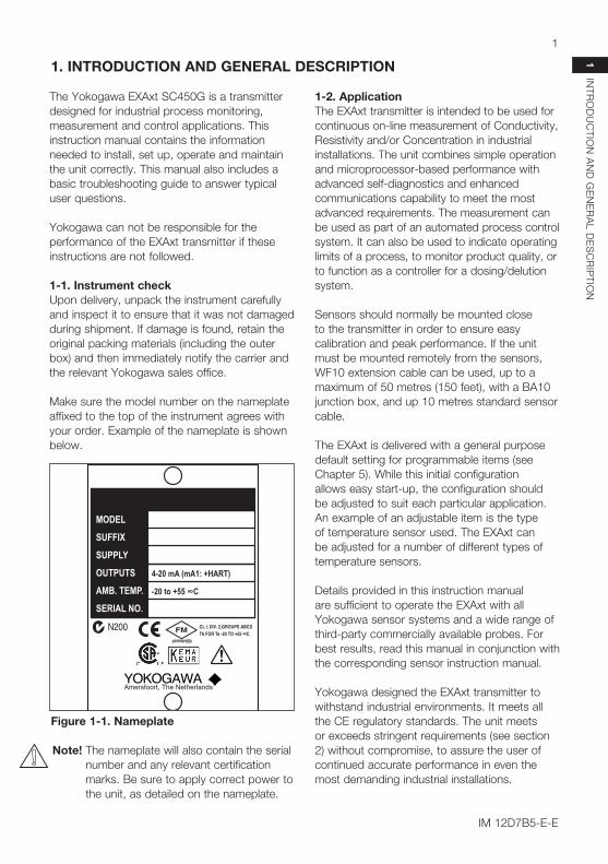
1-1. Instrument checkUpon delivery, unpack the instrument carefully and inspect it to ensure that it was not damaged during shipment. If damage is found, retain the original packing materials (including the outer box) and then immediately notify the carrier and the relevant Yokogawa sales office.

Make sure the model number on the nameplate affixed to the top of the instrument agrees with your order. Example of the nameplate is shown below.

Note! The nameplate will also contain the serial number and any relevant certification marks. Be sure to apply correct power to the unit, as detailed on the nameplate.

1-2. ApplicationThe EXAxt transmitter is intended to be used for continuous on-line measurement of Conductivity, Resistivity and/or Concentration in industrial installations. The unit combines simple operation and microprocessor-based performance with advanced self-diagnostics and enhanced communications capability to meet the most advanced requirements. The measurement can be used as part of an automated process control system. It can also be used to indicate operating limits of a process, to monitor product quality, or to function as a controller for a dosing/delution system.

Sensors should normally be mounted close to the transmitter in order to ensure easy calibration and peak performance. If the unit must be mounted remotely from the sensors, WF10 extension cable can be used, up to a maximum of 50 metres (150 feet), with a BA10 junction box, and up 10 metres standard sensor cable.

The EXAxt is delivered with a general purpose default setting for programmable items (see Chapter 5). While this initial configuration allows easy start-up, the configuration should be adjusted to suit each particular application. An example of an adjustable item is the type of temperature sensor used. The EXAxt can be adjusted for a number of different types of temperature sensors.

Details provided in this instruction manual are sufficient to operate the EXAxt with all Yokogawa sensor systems and a wide range of third-party commercially available probes. For best results, read this manual in conjunction with the corresponding sensor instruction manual.

Yokogawa designed the EXAxt transmitter to withstand industrial environments. It meets all the CE regulatory standards. The unit meets or exceeds stringent requirements (see section 2) without compromise, to assure the user of continued accurate performance in even the most demanding industrial installations.

1 IN

TRO

DU

CTIO

N A

ND

GE

NE

RA

L DE

SC

RIP

TION

Amersfoort, The Netherlands

MODEL

N200

SUPPLY

OUTPUTS

AMB. TEMP.

SERIAL NO.

4-20 mA (mA1: +HART)4-20 mA (mA1: +HART)

-20 to +55 ∞C -20 to +55 ∞C

SUFFIX

1

IM 12D7B5-E-E

1. INTRODUCTION AND GENERAL DESCRIPTION

Figure 1-1. Nameplate

2. GENERAL SPECIFICATIONS OF EXAXT SC450G

A) Input specifications : Two or four electrodes measurement with square wave excitation, using max 60m (200ft) cable (WU40/WF10) and cell constants from 0.005 to 50.0 cm-1

B) Input ranges Conductivity : 0.000 μS/cm - 2000 mS/cm Minimum : 1μS x c.c. (underrange 0.00 μS x c.c.) Maximum : 200 mS x c.c. (overrange 2000 mS x c.c.) Resistivity : 0.0 � U•cm - 1000 ] U•cm Minimum : 5Ω / c.c. (underrange 0.0 Ω/c.c.) Maximum : 1MΩ / c.c. (overrange 1000 MΩ/c.c.) Temperature Pt1000 : -20 to 250ºC Pt100 : -20 to 200ºC Ni100 : -20 to 200ºC NTC 8k55 : -10 to 120ºC Pb36 (JIS NTC 6k) : -20 to 120ºC

C) Accuracy Conductivity/resistivity : ≤ 0.5 % of reading Temperature : ≤ 0.3 ºC (≤ 0.4 ºC for Pt100) mA outputs : ≤ 0.02 mA Ambient temperature : 500 ppm/ºC influence : ± 0.05% /ºC Step respons : ≤ 4 sec for 90% (for a 2 decade step)

D) Transmission signals General : Two isolated outputs of 4-20 mA. DC with common negative

Maximum load 600Ω. Bi-directional HART® digital communication, superimposed on mA1 (4-20mA) signal

Output function : Linear or non-linear 21-step table for Conductivity/Resistivity, concentration or temperature

Control function : PID control Burnout function : Burn up (21.0mA) or burn down (3.6mA) to signal failure acc. NAMUR NE43 : Adjustable damping : Expire time Hold : The mA-outputs are frozen to the last/fixed value during calibration/

commissioning

E) Contact outputs General : Four SPDT relay contacts with display indicators Switch capacity : Maximum values 100 VA, 250 VAC, 5 Amps.

Maximum values 50 Watts, 250 VDC, 5 Amps. Status : High/Low process alarms, selected from conductivity, resistvity,

concentration or temperature. Configurable delay time and hysteresis : PID duty cycle or pulsed frequency control : FAIL alarm Control function : On / Off : Adjustable damping : Expire time

2

IM 12D7B5-E-E

2 G

EN

ER

AL S

PE

CIFIC

ATIO

NS

3

IM 12D7B5-E-E

Hold : The contacts are frozen to the last/fixed value during calibration/commissioning

Fail safe : Contact S4 is programmed as a fail-safe contact

F) Temperature compensation Function : Automatic or manual : Process compensation by configurable temperature coefficient, NaCl

curve, 13 pre-defined matrices or 2 user programmable matrices

G) Calibration : Semi-automatic calibration using pre-configured OIML (KCl) buffer tables, with automatic stability check. Manual adjustment to grab sample

H) Logbook : Software record of important events and diagnostic data readily available in the display

I) Display : Graphical Quarter VGA (320 x 240 pixels) LCD with LED backlight and touchscreen. Plain language messages in English, German, French, Spanish and Italian

J) Shipping details Package size : 293 x 233 x 230 mm (L x W x D) (11.5 x 9.2 x 9.1 inch) Package weight : app. 2.5 kg (5.5lbs)

K) Housing : Cast Aluminim housing with chemically resistant coating; Polycarbonate cover with Polycarbonate flexible window

: Protection IP66/ NEMA4X Colour : Silver grey SC450-A(D)-A : IP66 cable glands are supplied with the unit SC450-A(D)-U : NEMA4X blind plugs are mounted in the unused cable entry holes

and can be replaced by conduit fittings as required Pipe, Panel or Wall mounting using optional hardware

L) Power supply : 100-240 VAC (±10%). Max 10VA, 47-63Hz, 12-24 VDC (±10%), max 10W

M) Regulatory compliance EMC : Meets directive 89/336/EEC : Emission conform EN 55022 class A : Immunity conform IEC 61326-1 Low Voltage : Meets directive 73/23/EEC : Conform IEC 61010-1, UL61010C-1 and CSA 22.2 No. 1010.1,

Installation category II, Pollution degree 2 : Certification for cCSAus, Kema Keur and FM Class 1, Div. 2, Group

ABCD, T6 for Ta -20 to 55ºC (FM Pending)

N) Environment and operational conditions Ambient temperature : -20 to +55 ºC Storage temperature : -30 to +70 ºC Humidity : 0 to 90% RH (non-condensing) Data protection : EEPROM for configuration data and logbook. Lithium cell for clock Watchdog timer : Checks microprocessor Power down : Reset to measurement Automatic safeguard : Auto return to measuring mode when touchscreen is untouched for 10 min.

3-1. Installation and dimensions

3-1-1. Installation siteThe EXAxt 450 transmitter is weatherproof and can be installed inside or outside. It should, however, be installed as close as possible to the sensor to avoid long cable runs between sensor and transmitter. In any case, the cable length should not exceed 60 metres (197 feet). Select an installation site where:• Mechanical vibrations and shocks are

negligible• No relay/power switches are in the direct

environment• Access is possible to the cable glands (see

figure 3-1) • The transmitter is not mounted in direct

sunlight or severe weather conditions• Maintenance procedures are possible

(avoiding corrosive environments)

The ambient temperature and humidity of the installation environment must be within the limits of the instrument specifications. (See chapter 2).

3-1-2. Mounting methodsRefer to figures 3-2 and 3-3. Note that the EXAxt transmitter has universal mounting capabilities:

• Panel mounting using optional brackets• Surface mounting on a plate (using bolts

from the back)• Wall mounting on a bracket (for example, on

a solid wall)• Pipe mounting using a bracket on a

horizontal or vertical pipe (maximum pipe diameter 50 mm)

Model Suffix Code Option code DescriptionSC450G Conductivity/Resistivity transmitterPower - A AC version (85…265 VAC) - D DC version (9.6…30 VDC) - A Always AOptions / SCT*1 Predefined Tagnumber (text only) / Q Quality and Calibration Certificate / UM Universal Mounting kit (panel, pipe, wall)

Model code

*1 If the tagnumber is predefined with the purchase, Yokogawa will inscript the tagplate with the specified tagnumber, and program the tagnumber in the transmitter.

4

IM 12D7B5-E-E

3. INSTALLATION AND WIRING

3

144(5.67)

144(5.67")

24.5(1")

114.5(4.51")

27(1.06")

M20

min.185 (7.25)

min

.195

(7.7

5)

138(5.43)

138(5.43)

M6

M6

M5

138

138

Figure 3-1. Housing dimensions and layout of glands

Figure 3-2. Option /UM. Universal mounting kit, panel mounting diagram

INS

TALLA

TION

AN

D W

IRIN

G

5

IM 12D7B5-E-E

Figure 3-3. Wall and pipe mounting diagram

80(3.15")

2x ø6.5(0.26")

4x ø10(0.4")

200(7.87")

70(2.75")

141.5(5.57")

2" ND. pipe

pipe mounting(horizontal)

pipe mounting(vertical)

wall mounting

OPTION /UM: Universal pipe/wall/panel mounting kit

3-2. Wiring3-2-1. PreparationRefer to figure 3-4. The relay contact terminals and power supply connections are under the screening (shielding) plate. These should be connected first. Connect the sensor, outputs and HART® communication connections last.

To open the EXAxt 450 for wiring:1. Loosen the four frontplate screws and swing

open the cover.2. The upper terminal strip is now visible.3. Remove the screen (shield) plate covering

the lower terminal strip.4. Connect the power supply and contact

outputs. Use the three glands at the back for these cables.

Always replace the screen plate over the power supply and contact terminals for safety reasons and to avoid interference.

5. Put back (replace) the screen (shield) plate over the lower terminals.

6. Connect the analog output(s), the sensor inputs, and, if necessary, the HART® wiring and input contact.

7. Use the front three glands for analog output, sensor inputs, contact input and HART® wiring (see figure 3-5).

8. Swing back the cover and secure it with the four screws.

9. Switch on the power. Commission the instrument as required or use the default settings.

WARNING

Figure 3-4. Internal view of EXA wiring compartment

LCD bracket

connector for (future) software updatesinput terminal block

protective shield bracketM20 glands

output terminal block

6

IM 12D7B5-E-E

potentio- meter

High voltage section

Contact(S1, S2)outputcables

mAcables

Contact(S3, S4)outputcables

SensorCables

Inputcontact

Powercable

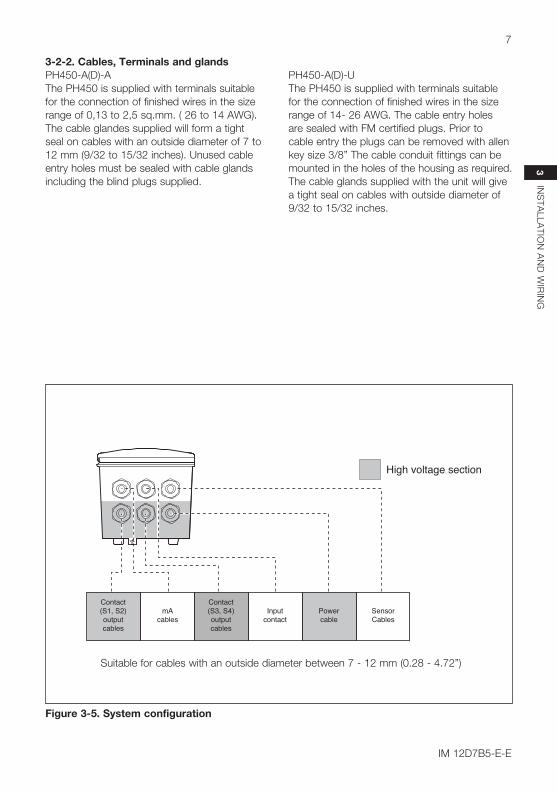
Suitable for cables with an outside diameter between 7 - 12 mm (0.28 - 4.72”)

Figure 3-5. System configuration

3 IN

STA

LLATIO

N A

ND

WIR

ING

7

IM 12D7B5-E-E

3-2-2. Cables, Terminals and glandsPH450-A(D)-AThe PH450 is supplied with terminals suitable for the connection of finished wires in the size range of 0,13 to 2,5 sq.mm. ( 26 to 14 AWG). The cable glandes supplied will form a tight seal on cables with an outside diameter of 7 to 12 mm (9/32 to 15/32 inches). Unused cable entry holes must be sealed with cable glands including the blind plugs supplied.

PH450-A(D)-UThe PH450 is supplied with terminals suitable for the connection of finished wires in the size range of 14- 26 AWG. The cable entry holes are sealed with FM certified plugs. Prior to cable entry the plugs can be removed with allen key size 3/8” The cable conduit fittings can be mounted in the holes of the housing as required. The cable glands supplied with the unit will give a tight seal on cables with outside diameter of 9/32 to 15/32 inches.

3-3. Wiring the power supply3-3-1. General precautionsMake sure the power supply is switched off. Also, make sure that the power supply is correct for the specifications of the EXAxt and that the supply agrees with the voltage specified on the textplate.

Local health and safety regulations may require an external circuit breaker to be installed. The instrument is protected internally by a fuse. The fuse rating is dependent on the supply to the instrument. The 250 VAC fuses should be of the “time-lag” type, conforming to IEC127.

Fuse ratings:Power supply Fuse type9.6-30VDC, 10W max 1A/250V, Slow85-265VAC, 10VA max 0.5A/250V, SlowRefer to the service manual for fuse replacement.

3-3-2. Access to terminal and cable entryTerminals 1, 2 and 3 are used for the power supply. Guide the power cables through the gland closest to the power supply terminals. The terminals will accept wires of 2.5 mm2 (14 AWG). Always use cable finishings if possible.

3-3-3. AC powerConnect terminal L1 to the phase line of the AC power and terminal N to the zero line. See figure 3-8 for the power ground. This is separated from input ground by a galvanic isolation.

3-3-4. DC powerConnect terminal 1 to the positive outlet and terminal 2 to the negative outlet. Terminal 3 is for the power ground. This is separated from input ground by a galvanic isolation. A 2-core screened cable should be used with the screen connected to terminal 3. The size of conductors should be at least 1.25 mm2. The overall cable diameter should be between 7 & 12 mm.

S1

S2

S4

S3

FRONT GLANDS REAR GLANDS

Sensor

outputsignals

HART

Contactoutput

Contactoutput

Power

Contact input

mA1

mA2

Figure 3-6. System configuration

8

IM 12D7B5-E-E

3

3-3-5. Grounding the housingFor the safety of the user and to protect the instrument against interference, the housing should always be connected to ground. This has to be done by a large area conductor. This cable can be fixed to the rear of the housing or by using the internal ground connections using a braided wire cable. See figure 3-8.

3-3-6. Switching on the instrumentAfter all connections are made and checked, the power can be switched on from the power supply. Make sure the LCD display comes on. After a brief interval, the display will change to the measured value. If errors are displayed or a valid measured value is not shown, consult the troubleshooting section (Chapter 8) before calling Yokogawa.

32 31 33 42 41 43 52 51 53 72 71 73NC C NO NC C NO NC C NO NO C NC

S1 S2 S3CONTACTS S4

250V / 5AAC / DC

100VA / 50W

(fail-safe)

Figure 3-7. Input and output connections

Figure 3-8-a. External grounding Figure 3-8-b. Internal grounding

63 66 65 61 22 21 12 15 16- + - +

mA OUTPUTS

62 11 13

TEMPmA2SHLD

CONTACT SENSOR(S)REFER TO INSTRUCTION MANUAL FOR CONNECTIONS SC

mA1(+HART)

14

ELECTRODEINNER INNEROUTER OUTER+ -

2N

1L

POWER100-240 VAC/10 VA/47-63 HzFUSE: 500 mA/250 VAC/T

AC

INS

TALLA

TION

AN

D W

IIRIN

G

9

IM 12D7B5-E-E

3-4. Wiring the contact signals3-4-1. General precautionsThe contact output signals consist of voltage-free relay contacts for switching electrical appliances (SPDT). They can also be used as digital outputs to signal processing equipment (such as a controller or PLC). It is possible to use multi-core cables for the contact in and output signals and shielded multi-core cable for the analog signals.

3-4-2. Contact outputs.The EXAxt 450 unit’s four contacts (switches) that can be wired and configured to suit user requirements. Contact S4 is programmed as a fail-safe contact. Please refer to section 5-7, Contact output setup for functionality description.

Alarm (limits monitoring)Contacts configured as “ALARM” can be energized when limits are crossed.

FailContacts configured as “FAIL” will be energized when a fail situation occurs. Some fail situations are automatically signaled by the internal diagnostics (electronics) of the transmitter. Others can be configured by the user (see section 5-11 Error Configuration). By pressing the “INFO” button on the main screen the user is given an explanation as well as a remedy for the current fail situation.Always connect the fail contact to an alarm device such as a warning light, alarm bell or displayed on an annunciator.

* When a fail situation occurs which is related to the parameter associated with the contact (Conductivity, Resistivity, Concentration or temperature) the contact will go to NC. When the fail situation is not related to the parameter associated with the contact the contact will remain in the state it is currently in.

3-5. Wiring the mA-output signals3-5-1. General precautionsThe analog output signals of the EXAxt transmit low power standard industry signals to peripherals like control systems or strip-chart recorders (Figure 3-6).

3-5-2. Analog output signalsThe output signals consist of active current signals of 4-20 mA. The maximum load can be 600 ohms on each.

It is necessary to use screening/shielding on the output signal cables. Terminal 63 is used to connect the shielding.

“ALARM” Contact “FAIL” Contact

Power Off NC NC

Power On NC NC

Alarm NO NC

Fail NC NO

Fail and Alarm NC* NO

HOLD** NC NC

10

IM 12D7B5-E-E

3

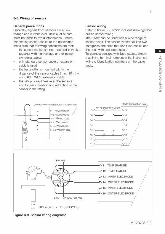
Figure 3-9. Sensor wiring diagrams

3-6. Wiring of sensors

General precautionsGenerally, signals from sensors are at low voltage and current level. Thus a lot of care must be taken to avoid interference. Before connecting sensor cables to the transmitter make sure that following conditions are met: – the sensor cables are not mounted in tracks

together with high voltage and or power switching cables

– only standard sensor cable or extension cable is used

– the transmitter is mounted within the distance of the sensor cables (max. 10 m) + up to 60m WF10 extension cable.

– the setup is kept flexible at the sensors end for easy insertion and retraction of the sensor in the fitting.

Sensor wiringRefer to figure 3-9, which includes drawings that outline sensor wiring.The EXAxt can be used with a wide range of sensor types. The sensor system fall into two categories, the ones that use fixed cables and the ones with separate cables.To connect sensors with fixed cables, simply match the terminal numbers in the instrument with the identification numbers on the cable ends.

INS

TALLA

TION

AN

D W

IIRIN

G

11

IM 12D7B5-E-E

3-6-1. Sensor cable connections using junction box (BA10) and extension cable (WF10)

Where a convenient installation is not possible using the standard cables between sensors and transmitter, a junction box and extension cable may be used. The Yokogawa BA10 junction box

and the WF10 extension cable should be used. These items are manufactured to a very high standard and are necessary to ensure that the specifications of the system can be met. The total cable length should not exceed 50 metres (e.g. 5 m fixed cable and 55 m extension cable).

14 Overall Screen

1112

12

1314

1416

15

1314

1416

15

17

1117

11 Red12 Blue

15 Core 16 ScreenWhite Co-axial cable

13 Core 17 ScreenBrown Co-axial Cable

17 (screen)

14 (overall screen)

12 (blue)

11 (red)

13 (core)

16 (screen)

15 (core)Co-axial cable

(white) Co-axial cable(brown)

11

12

13

14

15

16

17

11

12

13

14

15

16

17

BA10 WF10 EXA TRANSMITTER / CONVERTER

Figure 3-10. Connection of WF10 extension cable and BA10 junction box

12

IM 12D7B5-E-E

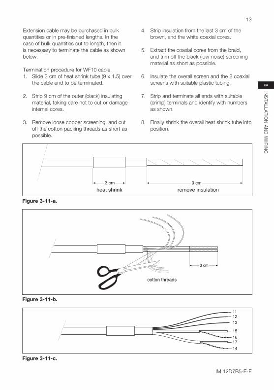
Extension cable may be purchased in bulk quantities or in pre-finished lengths. In the case of bulk quantities cut to length, then it is necessary to terminate the cable as shown below.

Termination procedure for WF10 cable.1. Slide 3 cm of heat shrink tube (9 x 1.5) over

the cable end to be terminated.

2. Strip 9 cm of the outer (black) insulating material, taking care not to cut or damage internal cores.

3. Remove loose copper screening, and cut off the cotton packing threads as short as possible.

4. Strip insulation from the last 3 cm of the brown, and the white coaxial cores.

5. Extract the coaxial cores from the braid, and trim off the black (low-noise) screening material as short as possible.

6. Insulate the overall screen and the 2 coaxial screens with suitable plastic tubing.

7. Strip and terminate all ends with suitable (crimp) terminals and identify with numbers as shown.

8. Finally shrink the overall heat shrink tube into position.

Figure 3-11-a.

3 cmheat shrink

9 cmremove insulation

Figure 3-11-b.

3 cm

cotton threads

Figure 3-11-c.

111213

15161714

3 IN

STA

LLATIO

N A

ND

WIIR

ING

13

IM 12D7B5-E-E

4-1. Main display functions

Figure 4-1. Main display

4-2. Trending graphicsPressing the button changes the display into a graphical mode in which the average measured value is shown on a time scale. The “Live” value is also digitally displayed in a text box. The time scale ( X-axis) and the primary value scale (Y-axis) are set in the “DISPLAY SETUP” menu. The full screen displays a trend of 51 points that represent the average of the selected time interval. The analyzer samples the measurement every second. The trending graphic also shows the maximum and minimum measured value in that interval. For example if the time scale is set to 4 hours, then the trend is shown for 4 hours prior to the actual measurement. Each point on the trend line represents the average over 4*60*60/51= 282 measurements (seconds).

4-3. Zoom in on detailsThis button gives access to the diagnostic information of the analyzer. The following messages will appear under normal (default) conditions: Zoom in on Details

Maximum

Minimum

Minimum

Maximum

Average

Live reading

SC

SC

T

120.0

90.0

60.0

30.0 109.3 µS/cm

450

Figure 4-2. Trend screen

14

IM 12D7B5-E-E

- Home key back to mainscreen.- One level up.

- Scroll choices (grey means deactivated).- Enter selected data or choice.

First zoom screen gives you inside into the parameters involving current measurement. All following zoom screens give additional information about the device and lead to logbook data.

Next

NextNext

Next

Figure 4-3. Detail screen

4. OPERATION OF EXAXT SC450G

4

4-3-1. actual mA1 = the current output in mA of the first current output, which is defined as mA1. The range and function of this mA output can be set in: Routing: Commissioning >> Output setup >> mA1

4-3-2. actual mA2 = the current output in mA of the second current output, which is defined as mA2. The range and function of this mA output can be set in:Routing: Commissioning >> Output setup >> mA2

4-3-3. S1/S2/S3/S4 = the current state of contacts 1 to 4. The functions and settings of the contacts can be set in: Routing: Commissioning >> Output setup >> S1/S2/S3/S4

4-3-4. C.C. (factory) = the nominal cell constant as determined by the factory calibration during production. This value is set during commissioning, and is found on the nameplate of the sensor or the calibration certificate.Routing: Commissioning >> Measurement setup >> Configure sensor

4-3-5. C.C. (adjusted) = the calibrated cell constant. When the cell constant of the system is adjusted on-line by grab sample or by calibrated solution technique, the new cell constant is recorded here. This value should not deviate greatly from the original factory calibration. In the event that there is a significant discrepancy seen between this reading and the C.C. (factory) value, the sensor should be checked for damage and cleanliness.Routing is via the “Calibration” menu.

4-3-6. Temp. comp 1 = the chosen temperature compensation method for the primary measurement.Routing: Commissioning >> Measurement setup >> Temp.compensation

4-3-7. Temp. comp 2 = the chosen temperature compensation method for the secondary measurement.Note: This does not imply two separate measurements. There is the possibility to set two separate compensation methods so that two different stages of the same process can be monitored accurately. An example is process/cleaning fluid interface.Routing: Commissioning >> Measurement setup >> Temp.compensation

4-3-8. Polarization = the polarization ismeasured by the input circuitry. Monitoring this figure gives a guide to progressive fouling of the sensor.

4-3-9. Sensor ohms = the input measurement as an uncompensated resistance value.

4-3-10. Last calibrated at = the date of the last calibration

4-3-11. Calibration due at = the date scheduled for the next calibration. This field is determined by the calibration interval.Routing: Commissioning >> Measurement setup >> Calibration settings

4-3-12. Projected calibration at = a diagnostic output, showing a time frame when the unit should next be maintained according to the sophisticated self-diagnostic tools built into the EXAxt software (for example >12 months, 3-6 months or 0-1 month). The analyzer checks the rate of polarization every 24 hours. If a clear increase of polarization is observed, the user is notified when a next calibration should take place. Prior to calibration the sensor should be well cleaned and rinsed.

4-3-13. Serial number = serial number of the transmitter.

4-3-14. Software revision = the revision level of the software in the instrument.

OP

ER

ATIO

N O

F EX

Axt S

C450G

15

IM 12D7B5-E-E

4-3-15. HART Device revisionSometimes the firmware of a device is updated in a way that the communication file (HART DD) need revision too. In this case the revision level is increased by one. The revision level of the HART DD must match the revision level of the Firmware. The revision level is expressed by the first two characters of the filename. The following files should be used when the HART Device revision level is 2.(0201.aot, 0201.fms, 0201.imp, 0201.sym)

4-3-16. LogbookThe EXAxt contains several logbooks to store historical information on events, changed settings and calibrations. The logbooks have been categorized to simplify the retrieval of this information.

Calibration will give information of previous calibrations. This logbook is useful as one now can1) Monitor the sensor performance over time.2) Monitor the sensor(s) lifetime.

Sensor will give all historical information on parameter settings concerning the sensor(s). The events logged in this logbook are user definable. This is done in: Commissioning >> Configure Logbook >> Sensor Logbook.

Predictive maintenance. If the sensor diagnostics of the EXAxt are enabled, the diagnostics are saved into this logbook.

For the EXAxt SC450G, the polarization (due to fouling) is stored once a day. This information can be used for (predictive) maintenance schedules as the polarization is a measure of fouling and the sensor should be kept clean for best results.

Settings wil give all history information on parameter settings concerning the analog outputs (mA1/mA2) and contact (S1…S4). This logbook is useful to trace back differences in performance due to changed settings. The events logged in this logbook are user definable. This is done in: Commissioning >> Configure Logbook >> Settings Logbook – mA and/or Settings Logbook – contact

mA1/mA2 shows all (dynamic) events concerning the analog outputsS1/S2/S3/S4 shows all (dynamic) events concerning the contacts.

Each HMI screen can contain up to 5 events. As each logbook can contain 50 events in total, one can access previous events by selecting another page 1 to 10.

4.3.17. Trouble shooting If you contact the local sales/ service organization the serial number and software revision is necessary information. Without that information it is impossible to help you. It is also very useful to report all the information that you find on the zoom-in display.

4-4. Information functionIn this field an information sign , a warning sign

or a fail sign can appear. Pushing this button, the user gets detailed information about the status of the sensor or the instrument if applicable. See troubleshooting (chapter 8) for further details.

4-5. Setup-Calibration & commissioningBy pressing the setup key, you get access to the operating system of the transmitter based on menus and submenus.

Browse through the list using the key till you find the required menu and press the key to enter this menu. It is also possible to press on the or symbol found beside the menu item.

4-6. Secondary- primary value display switch

Pressing on this text block automatically switches the secondary value to the main display (Large font size).

25.0

16

IM 12D7B5-E-E

4

“RE

TUR

N K

EY

” ex

it to

pre

viou

s di

spla

y

Main display

Primary setup display

Commisioning menu display

Instrument in HOLD

4-7. Navigation of the menu structure

OP

ER

ATIO

N O

F EX

Axt S

C450G

17

IM 12D7B5-E-E

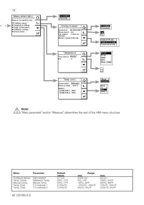
Menu Parameter Default Range values min. max. Configure Sensor Cell constant 0.1 cm-1 0.005 cm-1 50 cm-1 Temp. Comp. Reference Temp. 25ºC, 77ºF 0ºC, -4ºF 100ºC, 212ºF Manual Comp. Manual Temp. 25ºC, 77ºF -20ºC, 32ºF 250ºC, 482ºF Temp. Coef T.C.methods 1 2.10%/ºC -10%/ºC, -18%/ºF 10%/ºC, 18%/ºF Temp. Coef T.C.methods 2 2.10%/ºC 0%/ºC, 0%/ºF 3.5%/ºC, 2%/ºF

Note!“Main parameter” and/or “Measure” determines the rest of the HMI menu structure

18

IM 12D7B5-E-E

5

Measurement setupMain parameterChoose the required parameter, either conductivity or resistivity. If the main parameter is changed the instrument will reset main display settings, units and recalculate several values. The menu structure will change accordingly.

5-1. Configure sensor Sensor typeChoose the sensor type used. Normally conductivity and/or resistivity measurements are done with 2-electrode type sensors. At high conductivity ranges, polarization of the electrodes may cause an error in conductivity measurement. For this reason 4-electrode type sensors may be necessary.

Measuring unit /cm /mEither /cm or /m can be chosen here. The process values will be expressed in S/cm or S/m respectively, (Ω.cm or Ω.m in resistivity mode). Cell constant (factory)Cell constant given by factory calibration. Usually given on a label on the sensor or the calibration certificate. Only change this value in case a new sensor is used. By changing this value the actual cell constant is also changed.

MeasureProcess values to be measured can be selected to suit the user’s preference.: Conductivity only, Concentration only or one of both Conductivity and Concentration.Note: this choice is not available in Resistivity

mode.

5-2. Temperature settingTemperature ElementSelection of the temperature sensor used for compensation. The default selection is the Pt1000 Ohm sensor, which gives excellent precision with the two wire connections used. The other options give the flexibility to use a very wide range of other conductivity/resistivity sensors.

Temperature UnitCelcius or Fahrenheit temperature scales can be selected to suit the user’s preference.When the unit is changed all temperature related parameters and settings will be recalculated.

5-3. Temperature compensationCompensationTwo types of methods can be used here. Automatic for use of temperature element. Select one of the Temperature elements used. The other is a manual set temperature. The manual temperature that represents the process temperature must be set here.

Reference TemperatureChoose a temperature to which the measured conductivity (or resistivity) value must be compensated. Normally 25°C (77ºF) is used, therefore this temperature is chosen as the default value.

MethodTC In addition to the temperature coefficient calibration routine it is possible to adjust the compensation factor directly. If the compensation factor of the sample liquid is known from laboratory experiments or has been previously determined, it can be introduced here.Adjust the value between 0.00 to 3.50 % per °C. In combination with reference temperature a linear compensation function is obtained, suitable for all kinds of chemical solutions.NaCl Temperature compensation according NaCl curve. See appendix 1 for values.Matrix The EXAxt is equipped with a matrix type algorithm for accurate temperature compensation in various applications. Select the range as close as possible to the actual temperature/concentration range. The EXAxt will compensate by interpolation. If user defined 1 or user defined 2 is selected, the temperature compensation range for the adjustable matrix must be defined. See Appendix 6 for matrix interpolation.

Note! Extra information on temperature compensation is given in appendix 1.

5.MENU STRUCTURE COMMISSIONING

ME

NU

STR

UC

TUR

E C

OM

MIS

SIO

NIN

G

19

IM 12D7B5-E-E

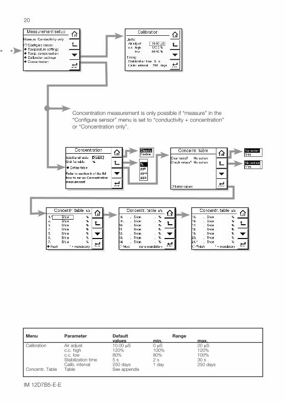
Menu Parameter Default Range values min. max. Calibration Air adjust 10.00 μS 0 μS 20 μS c.c. high 120% 100% 120% c.c. low 80% 80% 100% Stabilization time 5 s 2 s 30 s Calib. interval 250 days 1 day 250 days Concentr. Table Table See appendix

Concentration measurement is only possible if “measure” in the “Configure sensor” menu is set to “conductivity + concentration” or “Concentration only”.

20

IM 12D7B5-E-E

5-4. Calibration settingsAir adjust limitTo avoid cable influences on the measurement, a “zero” calibration with a dry sensor may be done. If a connection box (BA10) and extension cable (WF10) are being used, “zero” calibration should be done including this connection equipment. When using a 4-electrode sensor additional connections are required. Temporarily Interconnect terminals 13 & 14 with each other and 15 & 16 with each other before making the adjustment. This is necessary to eliminate the capacitive influence of the cables. The links should be removed after this step is completed. As the calibration is performed in air the resistivity is infinite (open connection). Higher conductivity values than the air adjust limit indicate the cell is not in air or is still wet. To prevent wrong air calibrations a limit must be given here.

c.c. high limitHigh limit of the cell constant expressed in % of nominal value. During calibration this value is used to check if the calibrated cell constant remains within reasonable limits.

c.c. low limitLow limit of the cell constant expressed in % of nominal value. During calibration this value is used to check if the calibrated cell constant remains within reasonable limits.

Stabilization timeDuring calibration the stability of the measurement is constantly monitored. When the value is within a bandwidth of 1% over a period of the stabilization time, the calibration is considered stable and the calibration may be completed.

Calibration IntervalA user defined interval in which a new calibration should take place. If the interval is exceeded the instrument will give a warning or a fail (user definable in error configuration 2/3)

5-5. ConcentrationConcentration has a direct relation with the conductivity value at reference temperature. This relation is built in every matrix which are used for temperature compensation. These can be found in:Commissioning >> Measurement setup >> Temp. compensation >> MethodBy selecting one of the matrices for temperature compensation directly gives the concentration value on the main display. If another temperature compensation method is chosen (NaCl or T.C.), the relation between the conductivity at reference temperature and the concentration is obtained from the “Concentration table”.

Additional tableThis 21x2 user defined concentration table is used to come to more accurate concentration values compared to the temperature compensation matrix. Enabling this additional table overrules the concentration values obtained from the matrix (if used).

Unit for tableThe way the concentration values are presented to the user. Changing the unit will not result in a re-calculation of the table.

5 M

EN

U S

TRU

CTU

RE

CO

MM

ISS

ION

ING

21

IM 12D7B5-E-E

mA2 similar structure to mA1

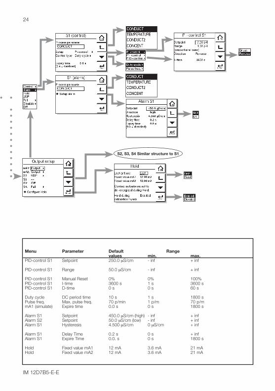
Menu Parameter Default Range values min. max. mA1 (control) Expire time 0.0 sec. 0 sec. 1800 sec. mA1 (output) Damping time 0.0 sec. 0 sec. 3600 sec. mA1 (simulate) Simulation perc. 50% 0% 100%

PID-control mA1 Setpoint 250.0 μS/cm - inf + inf PID-control mA2 Setpoint 25ºC/ºF - inf + inf PID-control mA1 Range 50.00 μS/cm - inf + inf PID-control mA2 Range 10ºC/ºF - inf + inf PID-control mA1 Manual Reset 0% 0% 100% PID-control I-time 3600 sec. 1 sec. 3600 sec. PID-control D-time 0 sec. 0 sec. 60 sec.

Linear mA1 0% Value 0 S/cm - inf + inf Linear mA2 0ºC/ºF - inf + inf Linear mA1 100% value 100 S/cm - inf + inf Linear mA2 100ºC/ºF - inf + inf Table Table mA1 see appendix - inf + inf

22

IM 12D7B5-E-E

5

5-6. mA output setupThe general procedure is to first define the function (control, output, simulate, off) of the output and second the process parameter associated to the output.Available process parameters depend on the selected “main parameter” and “measure”.Off : When an output is set off the

output is not used and will give an output of 4 mA

Control : A selection of P- PI- or PID controlManual : Static output required to maintainreset equilibrium state with setpointDirection : Direct

If the process variable is too high relative to the SP, the output of the controller is increased (direct action).

: Reverse If the process variable is too high relative to the SP, the output of the controller is decreased (reverse action).

Output : Linear or non linear table output. The table function allows the confi-guration of an output curve by 21 steps (5% intervals). In the main menu concentration can be selec-ted to set the concentration range.

Simulate : Percentage of output span. Normal span of outputs are limited from 3.8 to 20.5 mA

Fail safe : Contact S4 is programmed as a fail-safe contact.

Burn Low or High will give an output of 3.6 resp. 21 mA in case of Fail situation.

Note! When leaving Commissioning, Hold remains active until switched off manually. This is to avoid inappropriate actions while setting up the measurement

Proportional controlProportional Control action produces an output signal that is proportional to the difference between the Setpoint and the PV (deviation or error). Proportional control amplifies the error to motivate the process value towards the desired setpoint. The output signal is represented as a percentage of output (0-100%).

Proportional control will reduce but not eliminate the steady state error. Therefore, proportional Control action includes a Manual Reset. The manual reset (percentage of output) is used to eliminate the steady state error. Note! Any changes (disturbances) in the

process will re-introduce a steady state error. Proportional control can also produce excessive overshoot and oscillation. Too much gain may result in an unstable- or oscillating process. Too little gain results in a sustained steady state error. Gain = 1/Range. [PV units]

Integral ControlIntegral control is used to eliminate the steady state error and any future process changes. It will accumulate setpoint and process (load) changes by continuing to adjust the output until the error is eliminated. Small values of integral term (I-time in seconds) provide quick compensation, but increase overshoot. Usually, the integral term is set to a maximum value that provides a compromise between the three system characteristics of: overshoot, settling time, and the time necessary to cancel the effects of static loading (process changes). The integral term is provided with an anti windup function. When the output of PI portion of the controller is outside the control range (less than -5% or greater than 105%), the I-part is frozen.

Derivative controlThe control acts on the slope (rate of change) of the process value, thereby minimizing overshoot. It provides “rate” feedback, resulting in more damping. High derivative gains can increase the rizing time and settling time. It is difficult to realize in practice because differentiation leads to “noisy” signals.

SPPVe

+- ++ ++

+-

eRange

∫e dt1Ti

TddPVdt

z

Process

Controller

Actuator

Process

ME

NU

STR

UC

TUR

E C

OM

MIS

SIO

NIN

G

23

IM 12D7B5-E-E

Figure 5-1. Direct/Reverse action

S2, S3, S4 Similar structure to S1

Menu Parameter Default Range values min. max. PID-control S1 Setpoint 250.0 μS/cm - inf + inf PID-control S1 Range 50.0 μS/cm - inf + inf PID-control S1 Manual Reset 0% 0% 100% PID-control S1 I-time 3600 s 1 s 3600 s PID-control S1 D-time 0 s 0 s 60 s

Duty cycle DC period time 10 s 1 s 1800 s Pulse freq. Max. pulse freq. 70 p/min 1 p/m 70 p/m mA1 (simulate) Expire time 0.0 s 0 s 1800 s

Alarm S1 Setpoint 450.0 μS/cm (high) - inf + inf Alarm S2 Setpoint 50.0 μS/cm (low) - inf + inf Alarm S1 Hysteresis 4.500 μS/cm 0 μS/cm + inf

Alarm S1 Delay Time 0.2 s 0 s + inf Alarm S1 Expire Time 0.0. s 0 s 1800 s

Hold Fixed value mA1 12 mA 3.6 mA 21 mA Hold Fixed value mA2 12 mA 3.6 mA 21 mA

24

IM 12D7B5-E-E

Expire timeIf the output is over 100% for longer than the expire time, the output will return to 0%.

Damping timeThe response to a step input change reaches approximately 90 percent of its final value within the damping time.

Figure 5-2. Direct/Reverse action

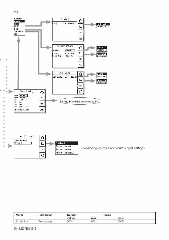
5-7. Contact output setputS1/S2/S3/S4Each Switch (contact) can have the following functions.1. Control : A selection of P- PI- or PID control2. Alarm : Low or high value Limits monitoring3. Hold : A hold contact is energised when

the instrument is in HOLD5. Fail : S4 is set as fail-safe contact. 6. Simulate : To test the operation of the contact,

simulate can be used. The contact can be switched on or off or a percentage of duty cycle can be entered (DC period time)

7. Off : Switch is not used.8. USP : USP/EU limits for WFI

Configure holdHold is the procedure to set the outputs to a known state when going into commissioning. During commissioning HOLD is always enabled, outputs will have a fixed or last value. During calibration the same HOLD function applies. For calibration, it is up to the user if HOLD is enabled or not.

Lifetime contactsOne should note that the lifetime of the contacts is limited (106) When these contacts are used for control (pulse frequency or duty cycle with small interval times) the lifetime of these contact should be observed. On/Off control is preferred over Pulse/duty cycle.

5

100

50

0

% controller output

Range

0.3 s

Maximum pulse frequency

50% pulse frequency

No pulses

0.3 s

Setpoint

Hys.

SC

off on off

Delay time Delay timet (sec)

100

50

0

ton toff

50% 50%

% controller output

Range

Duty cycle

ton > 0.1 sec

Duty cycle

toff > 0.1 sec

Duty cycle

Figure 5-4. Duty cycle control

Figure 5-5. Pulse frequency control

Figure 5-3. Alarm contact (on/off control)

100%

0%set

pointprocessvalue

Direct

100%

0%set

pointprocessvalue

Reverse

range

range

manualreset

manualreset

ME

NU

STR

UC

TUR

E C

OM

MIS

SIO

NIN

G

25

IM 12D7B5-E-E

power on power on power down normal opened contact activated S1, S2, S3 S4

S2, S3, S4 Similar structure to S1

Menu Parameter Default Range values min. max. Simulation Percentage 50% 0% 100%

(depending on mA1 and mA2 output settings)

26

IM 12D7B5-E-E

5

5-8. FailA fail contact is energized when a fail situation occurs. Fail situations are configured in secton 5-11. For SOFT Fails the contact and the display LED are pulsating. For HARD Fails the contact and the display LED are energized continuously. Only contact S4 is programmed as a fail-safe contact. This means that contact S4 will be de-energized when a fail situation occurs.

The contact reacts to Hard Fails Only

The contact reacts to Hard and Soft Fails

5-9. SimulateThe contact can be switched on/off or a percentage of output can be simulated. On/Off enables the user to manually switch a contact on or off. The percentage is an analogue value and represents the on time per period. The Duty Cyde Period time (see figure 5-4) is used as a period for percentage simulation. Note that the (simulated) settings of the contacts become visible in measuring mode and after HOLD has ended c.q. has been overruled. A warning is activated in case of a simulated output contact.

5-10. Water for Injection Monitoring (USP 645 and EU 0169).

Setting up EXA SC450 for WFI monitoring1. In Software Rev. 1.1, a function “USP detect”

is defined as Error Code on page 29 Error 2/3. This can be set to off/warn/fail according to your requirement. This function can be modified by the function “USP alarm limit” in %. This a percentage of the WFI conductivity value at that temperature that serves as safety margin. This is independent of what is being measured. The display shows this error when the water quality exceeds the WFI conductivity limits as set in stage 1.

2. We have introduced uncompensated conductivity in the DISPLAY menu. In the LCD display the user can read the temperature and the raw conductivity to compare his water quality with the WFI table.

3. We have added a USP function to the contact allocation. Only contact 1 can be selected as USP alarm if the function USP detect has been selected. The contact closes when the USP limit is reached.

Figure 5-6. USP Safety Margin

Limit of uncompensated conductivity as function of temperature as defined for WFI. USP Alarm Limit set as 20 % will close the contact at 80 % of the conductivity value at all temperatures.For example, if the temperature is 64 ºC. and the safety margin is adjusted for 20%, then the contact closes at 0.8 x 2.2 μS/cm. = 1,76 μS/cm. (2.2 μS/cm is the WFI limit at 64ºC). In resistivity mode the contact will close at an uncompensated resistivity of 1/1.76 μS/cm. = 0,568 Mohm.Recommended Commissioning settings when monitoring WFI in a > 80 ºC WFI installation.

Commissioning

Measurement Set up Measure Conductivity only Temp Compensation automatic Conductivity 1 None Error Configuration (Errors 2/3) USP Limit exceeded Warn

Output Setup S1 USP S2 Alarm Parameter Temperature Setpoint 80 C Direction Low Delay Time 0.2 s Expiry Time 0 (disabled)

5-11s. Input contactsThe terminal of the SC450G provides for an input contact (see Figure 3-7). This input contact can be used to switch the range of the outputs. The range can be increased by 1 decade.

Hard fail only

Hard + soft fail

ME

NU

STR

UC

TUR

E C

OM

MIS

SIO

NIN

G

27

IM 12D7B5-E-E

0,0

0,5

1,0

1,5

2,0

2,5

3,0

3,5

25 50 75 100C

mS

/cm

USPSafety Margin

Menu Parameter Default Range values Low High Errors1/3 Cond. High Limit 250 mS 0 mS 500 mS Errors1/3 Cond. Low Limit 1.000 μS 0.00 μS 500 mS Errors1/3 Res. Low Limit 4Ω 0 10MΩ Errors1/3 Res. Low Limit 1MΩ 0 10MΩ

28

IM 12D7B5-E-E

5

5-12. Error configurationErrors 1/3 ~ 3/3Errors are intended to notify the user of any unwanted situations. The user can determine which situations should be clasified as:FAIL, immidiate action is required. The process variable is not reliable.WARN, the process variable processes by the transmitter is still reliable at this moment, but maintenance is required in the near future.

“FAIL” gives a flashing “FAIL” flag in the main display. The contact configured as FAIL(Commissioning >> output setup)will be energized continuously. All the other contacts are inhibited. A Fail signal is also transmitted on the mA-outputs when enabled (burn high/low). (Commissioning >> output setup)

“WARN” gives a flashing “WARN” flag in the display. The contact configured as FAIL is pulsed. All the other contacts are still functional, and the transmitter continues to work normally. A good example is a time-out warning that the regular maintenance is due. The user is notified, but it should not be used to shut down the whole measurement.

5-13. Logbook configurationGeneralLogbook is available to keep an electronic record of events such as error messages, calibrations and programmed data changes. By reference to this log, users can for instance easily determine maintenance or replacement schedules.

In “Configure Logbook” the user can select each item he is interested in to be logged when the event occurs. This can be done for three separate logbooks. Each logbook can be erased individually or all at once. Enable the ”Warn if Logbook full” when you would like to be warned when the logbook is almost full.

The content of the logbook(s) can also be retrieved from the transmitter using the “EXAxt Configurator” software package which can be downloaded from the Yokogawa Europe website.

Flashing “Fail” flag in main display

Flashing “Warn” flag in main display

ME

NU

STR

UC

TUR

E C

OM

MIS

SIO

NIN

G

29

IM 12D7B5-E-E

Menu Parameter Default Range values Low High HART Network address 0 0 15

30

IM 12D7B5-E-E

5-14. Advanced setupDefaultsThe functionality of the EXAxt allows to save and load defaults to come to a known instrument setting. The EXAxt has both factory and user defined defaults.After a “load default” the instrument will reset. The following parameters are not included in the defaults:1. X-axis timing2. Auto return (10 min / disabled)3. Tag4. Passwords5. Date and time6. Language7. The contents of all logbooks8. HART parameters (address, tag, descriptor, message)

TagA tag provides a symbolic reference to the instrument and is defined to be unique throughout the control system at one plant site. A tag can contain up to 12 characters. If the instrument is purchased with the /SCT option, the TAG is pre-programmed with the specified tagnumber.

PasswordsCalibration and Commissioning may be separately protected by a password. By default both passwords are empty. Entering an empty password results in disabling the password check.A password can contain up to 8 characters.When a password is entered for the calibration and commissioning a 4-digit operator ID can be entered. One can also leave the ID empty.

Date/timeThe Logbooks and trend graph use the clock/calendar as reference. The current date and time is set here. The current time is displayed in the third “zoom” menu.

Note! The fixed format is YYYY/MM/DD HH:MM:SS

HARTThe address of the EXAxt in a HART network can be set. Valid addresses are 0...15.

Factory adjustmentThis menu is for service engineers only. This section is protected by a password.

Attempting to change data in the factory adjustment menu without the proper instructions and equipment, can result in corruption of the instrument setup, and will impair the performance of the unit.

5 M

EN

U S

TRU

CTU

RE

CO

MM

ISS

ION

ING

31

IM 12D7B5-E-E

Menu Parameter Default Range values Low High Y-axis Conduct low 0 μS/cm - inf + inf Y-axis Conduct high 500 μS/cm - inf + inf Y-axis Conduct 2 low 0 μS/cm - inf + inf Y-axis Conduct 2 high 500 μS/cm - inf + inf Y-axis Temp. low 0ºC, 32ºF - inf + inf Y-axis Temp. high 100ºC, 212ºF - inf + inf

32

IM 12D7B5-E-E

5-15. Display setupMain DisplayThe main display consists of three lines with Process Values. Each line is user definable with the restriction that each line should have a different Process Value. The default settings can be defined here. By pressing one of the two smaller process values, this will become the main process value in the main screen. Autoreturn will cause the main display to go to default setting.See also 4-6 Secondary to Primary Value display Switch.

Note! Configuration possibilities in the main and secondary display lines are determined by the choices made in the menu measurement Measurement setup >> Measurement

Additional textEach process value can be given an additional text containing up to 12 characters per text. This text is displayed on the main display next to the process value. This way the user can distinguish separate measurements.

X-axis TimingThe time range of the trend graph can be set from 15 minutes up to 14 days.

Y-axis LimitsThe ranges for each measurement need to be set according the application.

Auto ReturnWhen Auto return is enabled, the transmitter reverts to the measuring mode (main display) from anywhere in the configuration menus, when no button is pressed during the set time interval of 10 minutes. The HOLD flag will be cleared and all outputs will function normally!

5 M

EN

U S

TRU

CTU

RE

CO

MM

ISS

ION

ING

33

IM 12D7B5-E-E

6-1. GeneralThe nominal cell constant of a conductivity sensor is determined at the construction stage, because it is a factor set by the size of the electrodes, and their distance apart. A conductivity sensor does not change its cell constant during operation, as long as it remains undamaged, and clean. It is therefore vital that in any calibration check the first step should be to clean the sensor, or at least check its cleanliness. After cleaning ensure that the sensor is carefully rinsed in distilled water to remove all traces of the cleaning medium.

In the commissioning menu, the original sensor configuration will include the programming of the cell constant defined for the sensor at manufacture. Follow the routing below to the setup screen :Commissioning >> Measurement setup >> Configure sensor

The Calibration menu of the SC450G is provided for fine tuning the sensor setup, and checking and verification after a time in service.

Where 1st and 2nd compensations are referred to in this part of the menu, these provide alternatives for the “wet” calibration, designed to give the user the greatest flexibility.This does not mean that two cell constants can or should be calibrated, they are alternative routes to the same end!

6-2. Cell constant manualThe intention of this calibration routine is to fine tune a sensor for which only the nominal cell constant is known, or recalibrate a sensor that has been changed (or damaged) in the course of operation. Choose 1st or 2nd compensation to suit the calibration solution used. The solution should be prepared or purchased, meeting the highest standards of precision available. Allow the sensor to reach stable readings for both temperature and conductivity before adjusting to correspond to the calibration solution value. The setting of a cell constant for a new (replacement) sensor is also possible in this routine. This

avoids the need for entry into the commissioning mode, which may have another authorization (password) level.

6-3. Cell constant automaticThis routine is built around the test method described in OIML (Organisation Internationale de Metrologie Legale). International Recommendation No. 56. It allows the direct use of the solutions prescribed in the test method, automatically selecting the appropriate temperature compensation. The look up table is used to find the appropriate conductivity reading for the measured temperature. See appendix 2 for OIML solutions

6-4. Air (zero) calibration With the clean dry cell in open air, the reading should be zero. The Air cal compensates for excess cable capacitance, and gives a better accuracy at low readings. This should be done for all installations during commissioning. After some time in service a dirty sensor may well show a high zero offset because of fouling. Clean the sensor and try again.

6-5. Sample calibrationWith the sensor in situ, a sample can be taken for laboratory analysis. Sample calibration records the time and reading, and holds these in memory until the analysis has been completed. The laboratory data can then be entered regardless of the current process value, without the need for calculations.

6-6. Temperature coefficient calibrationSimply input the solution conductivity at reference temperature (TR), after the sensor is allowed to stabilize at elevated temperature. EXAxt SC450G will calculate the temperature coefficient for you. The ideal temperature for this calibration, is the normal process value (TP). For good calibrations, the minimum span (TP TR) should be at least 2ºC. Note that the Temperature Compensation should be set to TC first.

34

IM 12D7B5-E-E

6. CALIBRATION

6

6-7. Temperature calibration In order to make the most accurate measurements, it is important to have a precise temperature measurement. This affects the display of temperature, and the output signal when used. More important, however, is the temperature compensation, and calibration accuracy.The temperature of the sensor system should be measured independently with a high precision thermometer. The display should then adjusted to agree with the reading (zero offset calibration only). For best accuracy this should be done as near to the normal operating temperature as possible.

6-8. Operation of hold function during calibration

EXAxt SC450G has a HOLD function that will suspend the operation of the control/alarm relays and mA-outputs.

During calibration, the user may choose to enable HOLD so that the output signals are frozen to a “last” or “fixed” value. Some users will choose to leave the outputs “live” to record the calibration event. This has implications for pharmaceutical manufacture, for example, where an independent record of calibrations is mandatory.

Press HOLD button on mainscreen, to remove the HOLD.The route for HOLD setup is Commissioning >> Output setup>> Configure Hold

6-9. General comments on SC calibrationa) SC sensors experience no drift except if they

are damaged or dirty

b) There are no good calibration solutions (like pH buffer solutions)

c) Solution calibration of SC demands laboratory technical skills

d) Solutions can be used to give a fair calibration check at higher conductivity

e) Solutions can NOT be used to check calibration at low conductivity.

f) Low conductivity solutions <10μS/cm absorb CO2 from the air very fast

g) Low conductivity measurement must be made only with air excluded

h) Apparatus must be scrupulously clean to avoid contamination

i) Sensor linearity is never a problem for lower values

j) A dirty sensor is prone to polarization

k) Polarization shows as a low side error at higher conductivity

l) A dirty sensor will often read perfectly at low conductivity

m) Wet calibration tests are best done towards the top of a sensor’s range

n) If the system responds correctly to the highest trip point, all is well

CA

LIBR

ATIO

N

35

IM 12D7B5-E-E

7-1. Periodic maintenance The transmitter requires very little periodic maintenance, except to make sure the front window is kept clean in order to permit a clear view of the display and allow proper operation of the touchscreen. If the window becomes soiled, clean it using a soft damp cloth or soft tissue. To deal with more stubborn stains, a neutral detergent may be used.

When you must open the front cover and/or glands, make sure that the seals are clean and correctly fitted when the unit is re-assembled in order to maintain the housing’s weatherproof integrity against water and water vapor.

Note! Never use harsh chemicals or solvents. In the event that the window does become heavily stained or scratched, refer to the parts list (Chapter 10) for replacement part numbers.

BatteryThe EXAxt transmitter contains a logbook feature that uses a clock to provide the timings. The instrument contains a lithium cell (battery) to support the clock function when the power is switched off. The cell has an expected working life of 10 years. Should this cell need to be replaced, contact your nearest Yokogawa service center.

FuseThere is a circuit board mounted fuse protecting the instrument. If you suspect that this needs to be replaced, contact your nearest Yokogawa service center.

7-2. Periodic maintenance of the sensor

Note! Maintenance advice listed here is intentionally general in nature. Sensor maintenance is highly application specific.

In general conductivity/resistivity measurements do not need much periodic maintenance. If the EXAxt indicates an error in the measurement or in the calibration, some action may be needed (ref. chapter 9 troubleshooting).

When a 2-electrode sensor has become fouled an insulating layer may be formed on the surface of the electrodes and consequently, an apparent increase in cell constant may occur, giving a measuring error.

This error is:2 x Rv/Rcel x 100 %where:Rv = the resistance of the fouling layerRcel = the cell resistance

Note! Resistance due to fouling or to polarization does not effect the accuracy and operation of a 4-electrode conductivity measuring system. If an apparent increase in cell constant occurs cleaning the cell will restore accurate measurement.

7-3. Cleaning methods1. For normal applications hot water with domestic washing-up liquid added will be effective.2. For lime, hydroxides, etc., a 5 ...10% solution of hydrochloric acid is recommended.3. Organic contaminants (oils, fats, etc.) can be easily removed with acetone.4. For algae, bacteria or moulds, use a solution of domestic bleach (hypochlorite).

* Never use hydrochloric acid and bleaching liquid simultaneously. The release of the very poisonous chlorine gas will result.

36

IM 12D7B5-E-E

7. MAINTENANCE

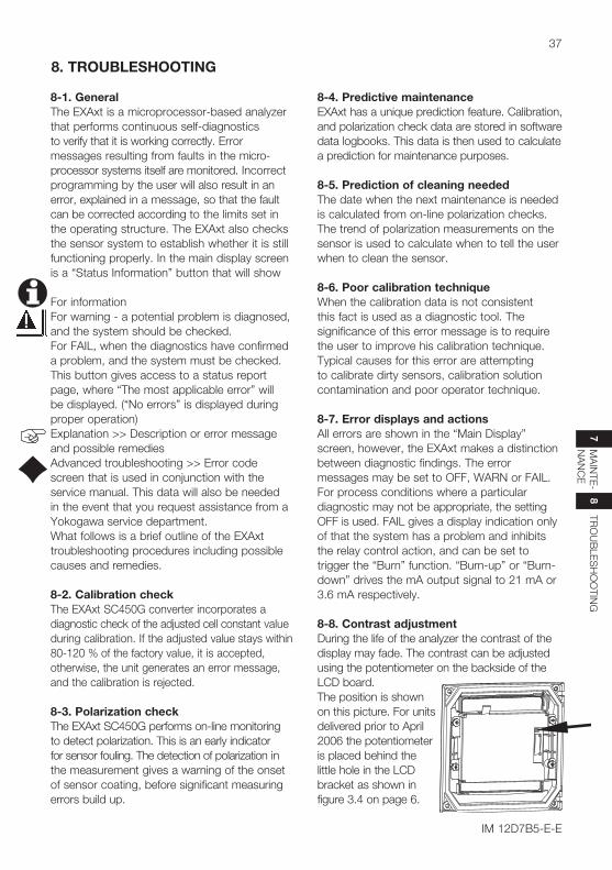
8-1. General The EXAxt is a microprocessor-based analyzer that performs continuous self-diagnostics to verify that it is working correctly. Error messages resulting from faults in the micro-processor systems itself are monitored. Incorrect programming by the user will also result in an error, explained in a message, so that the fault can be corrected according to the limits set in the operating structure. The EXAxt also checks the sensor system to establish whether it is still functioning properly. In the main display screen is a “Status Information” button that will show

For information For warning - a potential problem is diagnosed, and the system should be checked.For FAIL, when the diagnostics have confirmed a problem, and the system must be checked.This button gives access to a status report page, where “The most applicable error” will be displayed. (“No errors” is displayed during proper operation) Explanation >> Description or error message and possible remediesAdvanced troubleshooting >> Error code screen that is used in conjunction with the service manual. This data will also be needed in the event that you request assistance from a Yokogawa service department. What follows is a brief outline of the EXAxt troubleshooting procedures including possible causes and remedies.

8-2. Calibration checkThe EXAxt SC450G converter incorporates a diagnostic check of the adjusted cell constant value during calibration. If the adjusted value stays within 80-120 % of the factory value, it is accepted, otherwise, the unit generates an error message, and the calibration is rejected.

8-3. Polarization checkThe EXAxt SC450G performs on-line monitoring to detect polarization. This is an early indicator for sensor fouling. The detection of polarization in the measurement gives a warning of the onset of sensor coating, before significant measuring errors build up.

8-4. Predictive maintenanceEXAxt has a unique prediction feature. Calibration, and polarization check data are stored in software data logbooks. This data is then used to calculate a prediction for maintenance purposes.

8-5. Prediction of cleaning neededThe date when the next maintenance is needed is calculated from on-line polarization checks. The trend of polarization measurements on the sensor is used to calculate when to tell the user when to clean the sensor.

8-6. Poor calibration techniqueWhen the calibration data is not consistent this fact is used as a diagnostic tool. The significance of this error message is to require the user to improve his calibration technique. Typical causes for this error are attempting to calibrate dirty sensors, calibration solution contamination and poor operator technique.

8-7. Error displays and actionsAll errors are shown in the “Main Display” screen, however, the EXAxt makes a distinction between diagnostic findings. The error messages may be set to OFF, WARN or FAIL. For process conditions where a particular diagnostic may not be appropriate, the setting OFF is used. FAIL gives a display indication only of that the system has a problem and inhibits the relay control action, and can be set to trigger the “Burn” function. “Burn-up” or “Burn-down” drives the mA output signal to 21 mA or 3.6 mA respectively.

8-8. Contrast adjustmentDuring the life of the analyzer the contrast of the display may fade. The contrast can be adjusted using the potentiometer on the backside of the LCD board. The position is shown on this picture. For units delivered prior to April 2006 the potentiometer is placed behind the little hole in the LCD bracket as shown in figure 3.4 on page 6.

MA

INTE

- N

AN

CE

78

TRO

UB

LES

HO

OTIN

G

37

IM 12D7B5-E-E

8. TROUBLESHOOTING

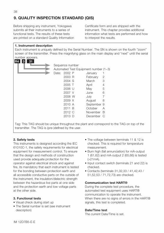
Sequence number Automated Test Equipment number (1~3) Date: 2002 P January 1 2003 R February 2 2004 S March 3 2005 T April 4 2006 U May 5 2007 V June 6 2008 W July 7 2009 X August 8 2010 A September 9 2011 B October A 2012 C November B 2013 D December C

Tag: This TAG should be unique throughout the plant and correspond to the TAG on top of the transmitter. The TAG is (pre-)defined by the user.

Before shipping any instrument, Yokogawa submits all their instruments to a series of functional tests. The results of these tests are printed on a standard Quality Information

Certificate form and are shipped with the instrument. This chapter provides additional information what tests are performed and how to interpret the results.

2. Safety tests This instruments is designed according the IEC 61010C-1, the safety requirements for electrical equipment for measurement control. To ensure that the design and methods of construction used provide adequate protection for the operator against electrical shock and against fire, its mandatory that each instrument is tested for the bonding between protection earth and all accessible conductive parts on the outside of the instrument, the insulation/dielectric strength between the hazardous live parts at one side and the protection earth and low voltage parts at the other side.

3. Functional tests• Visual check during start up• The Serial number is set (see instrument

description)

• The voltage between terminals 11 & 12 is checked. This is required for temperature measurement.

• Burn high (fail annunciation) for mA-output 1 (61,62) and mA-output 2 (65,66) is tested (>21mA).

• Input contact switch (terminals 21 and 22) is checked.

• Contacts (terminals 31,32,33 / 41,42,43 / 51,52,53 / 71,72,73) are checked.

Communication test HART®During the complete test procedure, the automated test equipment uses HART® communication to operate the instrument. When there are no signs of errors in the HART® signals, this test is completed.

Date/Time testThe current Date/Time is set.

R4 3 31

38

IM 12D7B5-E-E

9. QUALITY INSPECTION STANDARD (QIS)

1. Instrument descriptionEach instrument is uniquely defined by the Serial Number. The SN is shown on the fourth “zoom” screen of the transmitter. Press the magnifying glass on the main display and “next” until the serial number appears.

RESISTANCE DECADE BOX

SC450

- + G

HIGH RANGERESISTANCEDECADE BOX d

12

11

13

14

15

16

DECADE BOX 2 (Conductivity)

DECADE BOX 1 (Temperature)

mA Meter

300 Ω

+ -

24 VoltsDC Supply

9

Figure 9-1. Connection diagram for Test Procedure

QU

ALITY

INS

PE

CTIO

N

39

IM 12D7B5-E-E

4. Sensor input, linearity and accuracy testsAfter the instrument is initialized, the linearity and accuracy is tested. This is done by connecting adecade box between terminal 15 and 13. The measured “Sensor Ohms” are shown in the “Zoom” screen. By pressing the magnifying glass and “next” one will find the value.

5. Temperature accuracy testsThe EXAxt supports a number of temperature elements. All these elements are initialized and tested for accuracy. The resistor decade box is set to the following impedance values to accurately simulate the temperature element impedance.

-10 ºC 25 ºC 75 ºC 120 ºC 190 ºC 240 ºCPt1000 960.9 Ω 1097.4 Ω 1290.0 Ω 1460.6 Ω 1721.6 Ω 1904.6 ΩPt100 96.1 Ω 109.7 Ω 129.0 Ω 146.1Ω 172.2 Ω5k1 94.6 Ω 114.2 Ω 144.9 Ω 175.9 Ω 231.8 Ω8K55 47000.0 Ω 8550.0 Ω 1263.0 Ω 343.0 ΩPB36 9414.0 Ω 2179.0 Ω 421.2 Ω 133.3 Ω

6. mA-output accuracyThe EXAxt simulates a number of mA-output values. The accuracy of both mA-outputs is checked with a load of 300Ω. The ripple voltage over the 300Ω load is measured and should be within 30mV (RMS). With a load of 600Ω the instrument should still be able to transmit a signal of 22mA (no signal drop with maximum load).

7. Overall accuracy testsAll separate accuracy tests are performed. As all these accuracies will accumulate (or influence each other), an overall accuracy test is performed.

Note! That the instrument is set to default values as certain settings like temperature compensation will alter the transmitted signal. If one decides to perform an overall test, one can save current settings as user defined defaults before proceeding. Afterwards these settings can be restored from memory.

Note that we specify the environmental influences to our instruments in our specifications. These should be taken into account when performing an overall accuracy test.

8. ApprovalAll our instruments are designed and manufactured to the highest standards. All tests are performed under controlled ambient temperature and humidity by well trained employees.

40

IM 12D7B5-E-E

10. SPARE PARTS

(7) Front Cover assembly

(2) Pre&Dig Board

(4) LCD Zifcable

(9) Tag Plate

(5) Power Flatcable

(1) power board

(8) glandset

(6) fuse (at the backside)

(3) LCD Module

SP

AR

E P

AR

TS10

41

IM 12D7B5-E-E

Item Description Partnr1a Power board AC version K1548AF1b Power board DC version K1548DF2 Pre&dig board PH version K1548FE3 LCD module *) K1548ED4 LCD zifcable K1548JC5 Power flatcable K1548JD6a Fuse AC version (10 pcs.) K1548EF6b Fuse DC version (10 pcs.) K1548AM7 Cover assembly with gasket, screws and hingepins K1548MY8 Glandset (6 pcs. M20) plus 1 tule and Grommetset K1548MV9 Tagplate blank (incl. 2x M3) K1548MT10 Panelmounting kit K1541KR11 Pipe/wall mounting kit K1542KW12 Flashloader kit K1548FU

*) K1548EC= spare LCD for units delivered before may 2006 (SN=U5) K1548ED= spare LCD for units delivered after April 2006 and for all models 450- -U K1548EE= conversion kit for replacement of K1548EC by K1548ED. The kit includes LCD unit and

brackets. New Firmware version must be downloaded with Flash unit K1548FU.

Software version 1.10• Service menu moved to Advanced Setup - Factory Adjustment• introduced Service password that is unique per device (derived from S/N via an algorithm)• increased font size for unit in main screen• added the possibility to enter a four digit Operator-ID after entering the Calibration and

Commissioning password; this ID will be logged• HOLD flag has been given a ‘button’ look (can be pressed to deactivate HOLD)• After leaving Setup, the HOLD status is made equal to the situation before entering Setup• routing tags in Output Configuration screen longer then 12 characters will be shown correctly• result of Predictive Maintenance calculation shown as time frame (instead of date)• improved detection, analysis and handling of error 121 (unstable measurement)• improved error analysis (Eeprom error generated) for a completely uninitialized device• system errors during (re)start of device are now logged• fixed reset problem due to watchdog error caused by a full logbook (from 1.01)• display changes from 4 to 3 digits at 500 xS/cm (instead of 200)• added the possibility to configure any output contact as USP contact• polarization now shown without unit

Software version 1.20• Firmware update for new LCD (April 2006)• The pure water limit +25% is implemented in steps of 5 °C from 0 to 135 °C

42

IM 12D7B5-E-E

11. SOFTWARE HISTORY

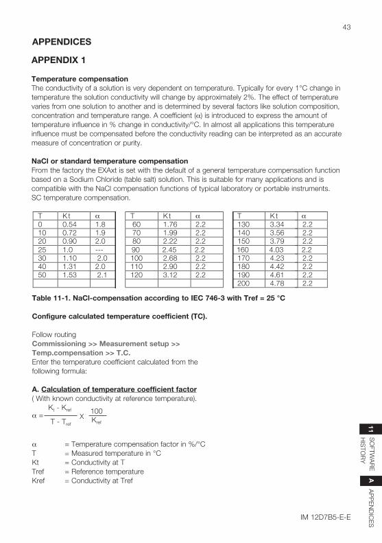
43

IM 12D7B5-E-E

Configure calculated temperature coefficient (TC).

Follow routing Commissioning >> Measurement setup >> Temp.compensation >> T.C.Enter the temperature coefficient calculated from the following formula:

A. Calculation of temperature coefficient factor( With known conductivity at reference temperature).

α = Temperature compensation factor in %/°CT = Measured temperature in °CKt = Conductivity at TTref = Reference temperature Kref = Conductivity at Tref

APPENDIX 1

Temperature compensationThe conductivity of a solution is very dependent on temperature. Typically for every 1°C change in temperature the solution conductivity will change by approximately 2%. The effect of temperature varies from one solution to another and is determined by several factors like solution composition, concentration and temperature range. A coefficient (α) is introduced to express the amount of temperature influence in % change in conductivity/°C. In almost all applications this temperature influence must be compensated before the conductivity reading can be interpreted as an accurate measure of concentration or purity.

NaCl or standard temperature compensationFrom the factory the EXAxt is set with the default of a general temperature compensation function based on a Sodium Chloride (table salt) solution. This is suitable for many applications and is compatible with the NaCl compensation functions of typical laboratory or portable instruments. SC temperature compensation.

Table 11-1. NaCl-compensation according to IEC 746-3 with Tref = 25 °C

Kt - Kref α =

T - Tref

100Kref

X

APPENDICES

AP

PE

ND

ICE

S

A S

OFTW

AR

E H

ISTO

RY

11

44

IM 12D7B5-E-E

Calculation exampleCalculate the temperature coefficient of a liquid from the following data. Conductivity 124.5 μS/cm at a liquid temperature of 18.0 °C and a conductivity 147.6 μS/cm at a liquid temperature of 31.0 °C.

Substituting the data in the above formula gives the following result.

Set the temperature coefficient in the SC450G converter.

147.6 - 124.5x 100= 1.298 %/Cα =

124.5(31.0 - 25) - 147.6(18.0 - 25)

Where T 1 , T 2 : liquid temperature (°C) K 1 : conductivity at T 1 (°C) K 2 : conductivity at T 2 (°C) Figure 11-1. Conductivity

B. Calculation of temperature coefficient factor(with two known conductivity values at different temperatures)Measure the conductivity of the liquid at two temperatures, one below the reference and above the reference temperature with the temperature coefficient set to 0,00%/°C and use the following equation to calculate a temperature coefficient (α).

KTKref =

1+α ( T - Tref )

K2 - K1

α =K1 ( T2 - Tref ) - K2 ( T1 - Tref )

K1 K2Kref = =1+α ( T1 - Tref ) 1+α ( T2 - Tref )

K1 (1 + α ( T2 - Tref )) = K2 (1 + α ( T1 - Tref ))

K1 · α ( T2 - Tref ) - K2 · α ( T1 - Tref ) = K2 - K1

45

IM 12D7B5-E-E

CheckingWhen the temperature coefficient already set is accurate, the conductivity to be displayed must be constant regardless of liquid temperature. The following check will make sure that the temperature coefficient already set is accurate.If, when the liquid temperature is lowered, a larger conductivity value is indicated, the temperature coefficient already set is too small.The opposite also applies. If a smaller conductivity value is indicated, the temperature coefficient already set is too large. In either case, change the temperature coefficient so that the conductivity no longer changes.

Matrix compensationThe compensation matrix is a table of temperature and conductivity values at differing concentrations. These values are used to calculate the temperature compensation applicable for a particular solution. Choose the component that you will be measuring in your application, and where appropriate the concentration range. The EXAxt will do the rest.

By following the routing:Commissioning>> Measurement setup>> Temp.compensation>> Matrixyou gain access to the Matrix selection area.

Matrices are available for the common mineral acids and bases. In addition Ammonia and Morpholine are included. In short by using the matrix method, specialist compensation is available for the majority of applications in the power industry, water treatment, and chemical manufacturing. The following matrices are available initially, but as with all Yokogawa products, we are continually striving to improve both the quality and technological content. Further solutions will be added to this list.

Ammonia 0..50 ppb 0..90˚C Ammonia 15..30% 10..50˚CMorpholine 0..500ppb 0..90˚CH2SO4 0..27% 0..100˚CH2SO4 39..85% -18..116˚CH2SO4 93..100% 10..90˚CNaOH 0..15% 0..100˚CNaOH 25..50% 0..80˚CHCl 0..200ppb 0..100˚CHCI 0..18% -10..65˚CHCI 24..44% -20..65˚CHNO3 0..25% 0..80˚CHNO3 35..88% -16-60˚C

AP

PE

ND

ICE

S

A

46

IM 12D7B5-E-E

The matrix can be cleared before entering new values. Next new matrix values can be entered as described above. The EXAxt can interpolate the matrix. During this process it will check if the matrix is completely ascending/descending. This is necessary as otherwise the lookup function can give two results for one temperature. If an error is found, the EXAxt will specify the location of the error as shown in the user interface screen “user defined 1/2”.

the backspace key should be used for deleting an individual matrix value.

An empty value is shown as

Temperature compensation matrix.

1. A minimum number of values is required to make interpolation possible. The highlighted values markes as are mandatory to enter.

Concent Tref T1 .... Tx .... T10 Sol1 C1 S1Tr S1T1 S1T10 .... Solx SxTx .... Sol10 C10 S10Tr S10T1 S10T10

2. Tref (reference temperature) is defined in the Temperature Compensation menu. If Tref is between T1 and T10 then the value of Tref needs to be entered as Tx (T2....T9)

concent Tref T1 .... Tx .... T10 Sol1 C1 S1Tr S1T1 S1T10 .... Solx .... Sol10 C10 S10Tr S10T1 S10T10

3. For every SxTx that is entered the following values become mandatory to enter: Cx, SxTr, SxT1, SxT10 and Tx

concent Tref T1 .... Tx .... T10 Sol1 C1 S1Tr S1T1 S1T10 .... Solx Cx SxTr SxT1 SxTx SxT10 .... Sol10 C10 S10Tr S10T1 S10T10

47

IM 12D7B5-E-E

APPENDIX 2

TDS readingsThe concept of Total Dissolved Solids (TDS) is widely used as an indication of the total solute concentration in water and is a widely accepted water quality standard. The determination is simply made by evaporation and weighing the residue. As the heat treatment converts the chemical properties of the solution, some solutes that contribute to the total conductivity will not be found in the residue. Also some combinations of solutes will become volatile at the drying temperature. The same applies for those solutes that do not contribute to the conductivity but do end up in de residue. When one (or a few) solute is dominant in the solution, these problems may be neglected and TDS will have a direct correlation with the conductivity. Next is a graph that shows the correlation between the specific conductance and concentrations (by weight) for six salts. The factor by which the conductivity should be multiplied to come to a TDS reading ranges from 0.4 to 0.7 up to a conductivity of 500 uS/cm. At a conductance of approximately 3000 uS/cm the range would be from 0.5 and 1.0.

The EXAxt 450 measures conductivity. This value can be used to display TDS values on the main display. One should use the additional concentration table. Please refer to section 5.5 for concentration measurement. The unit for the TDS reading can be set to ppb or ppb.

0 1000 2000 3000 4000 5000

1000

2000

3000

4000

5000

6000

7000

Concentration, mg/L

Spe

cific

con

duct

ance

, µS

/cm

, 25º

C

MgCI2 Na2SO4

MgSO4

CaCI2

NaCI2 KCI

AP

PE

ND

ICE

S

A

48

IM 12D7B5-E-E

APPENDIX 3

Calibration solutions for conductivity

Note! This section should be read in conjunction with the calibration section (Chapter 7) and the maintenance section (Chapter 8). The calibration (cell constant) of a sensor does not change unless the sensor is damaged.It can also appear to change because of coating of the electrodes, or partial blockage. Because these changes should be handled as described in the maintenance section, it does not make sense to regularly recalibrate the SC450G.

A calibration check, however, is another matter. When the objective is clearly defined as a diagnostic exercise a regular check can bring an extra level of security and confidence to the measurement.

Sensor damage, and/or coatings can be difficult to see and the calibration check can confirm their presence, by a deviation from the known solution conductivity. The remedial action should be to clean the sensor, and carefully check for blockage or damage (not simply to recalibrate).

Higher conductivity solutions should be used where possible. The lower the conductivity of the test solution, the easier it is to contaminate. Carbon dioxide from the air can be quickly absorbed to cause an error. All containers must be suitably clean, and all materials suitably pure. Outside of a well-equipped laboratory these conditions are hard to meet.

Also note that the check must be performed with due regard to the cell constant of the sensor, as it limits the effective working range. The documentation provided with the sensor should be consulted to determine its maximum working value. By using a checking solution close to the upper range limit of the sensor, the detection of contamination is better. A slightly contaminated sensor may read perfectly at lower conductivity, but show significant errors at higher values. This is caused by the early onset of polarization, the factor that limits the upper range of the sensor in any case. Polarization is seen in contaminated sensors, and it is for this reason that there is a sophisticated polarization check built into the SC450G. Details of this diagnostic tool are found in the troubleshooting section (Chapter 9).

EXAxt SC450G is programmed with the following table of conductivity of Potassium Chloride (KCl) solutions at 25°C. This is used in the Automatic Cell Constant setting calibration feature. (See chapter 7 on calibration) The table is derived from the Standards laid down in “International Recommendation No. 56 of the Organisation Internationale de Métrologie Legale”.

Table 5-2. KCl values at 25 °C

49

IM 12D7B5-E-E

Note!For resistivity measurement the standard resistivity units of the calibration solution can be calculated as follows:R = 1000/G (kΩ.cm if G = μS/cm)

Example: 0.001% weight R = 1000/21.4 = 46.7 kΩ.cm

Weight % mg/kg Conductivity0.001 10 21.4 µS/cm0.003 30 64.0 µS/cm0.005 50 106 µS/cm0.01 100 210 µS/cm0.03 300 617 µS/cm0.05 500 1.03 mS/cm0.1 1000 1.99 mS/cm0.3 3000 5.69 mS/cm0.5 5000 9.48 mS/cm1 10000 17.6 mS/cm3 30000 48.6 mS/cm5 50000 81.0 mS/cm

10 100000 140 mS/cm

Table 5-3. NaCl values at 25 °C

If it is more convenient, the user may make solutions from Sodium Chloride (NaCl or common table salt) with the help of the following relationship table. This table is derived from the IEC norm 746-3.

AP

PE

ND

ICE

S

A

50

IM 12D7B5-E-E

APPENDIX 4

Sensor selection for the EXAxt SC450G

Yokogawa supplies the following sensors, and their application is briefly described. All are compatible with the EXAxt SC450G, and the user must be aware of the sensor configuration for 2 or 4 electrodes, in order to set the converter correctly.

SC42-SP34 (&SX42-SX34) cc = 0.01 cm-1 2-electrode sensorThis sensor is the first choice for pure and ultra pure water measurements. From 0.055μS/cm up to 100μS/cm this is a perfect choice. The measuring range extends to at least 1000μS/cm, but there are better choices in that range.Almost exclusively used in flow fittings and sub-assemblies. FF40 and FS40. (The -SX sensors are screwed or flanged direct into the process pipework or tanks.)

SC4A-S(T)-XX-002...... cc = 0.02 cm-1 2-electrode sensorThis sensor is a good choice for pure and ultra pure water measurements. From 0.055μS/cm up to 50μS/cm this is a good choice. The measuring range extends to 500μS/cm, but there are better choices in that range. The “SC4A-” sensors make up a range that use compression adapters or specialized fittings, including retractable.

SC42-SP24 (&SX42-SX24) cc = 0.1cm-1 2-electrode sensorThis sensor should be used for clean and pure water measurements. From 0.2μS/cm up to 1 mS/cm the sensor is fine, with measurement up to 10 mS/cm possible, but there are better choices in that range. Mounting of these sensors is as for the ....-SP(X)34 series.

SC4A-S(T)-XX-010...... cc = 0.1 cm-1 2-electrode sensorThis sensor is a good choice for clean water measurements. From 0.5μS/cm up to 200μS/cm this is a good choice. The measuring range extends to 2000μS/cm, but there are better choices in that range. The “SC4A-” sensors make up a range that uses compression adapters or specialized fittings, including retractable.

SC42-EP15(D) cc = 1 cm-1 2-electrode sensorThis sensor is intended as a handy, short sensor. It is easy to fit in a branch (tee) on a pipeline, and is good for measurements where the precision is less critical than a convenient installation. The D version is particularly suited to food applications because of it’s cleanability. Range of application is from 10 μS/cm to 10 mS/cm.

SC42-EP14 cc = 1 cm-1 2-electrode sensorClean cooling and process water applications are where this sensor is used. The best range of application is 10μS/cm to 10mS/cm. It is better suited to flow through installations in FS40 and FF40 adapters and fittings, but it can also be used in dip tubes - FD40.

SC42-EP18 cc = 1 cm-1 4-electrode sensorCooling and process water applications are where this sensor is used, including light fouling. The best range of application is 100μS/cm to 100mS/cm. The four-electrode system copes with some contamination from the process, and eliminates the tendency for polarization to occur at the higher conductivity. It is better suited to flow through installations in FS40 and FF40 adapters and fittings, but it can also be used in dip tubes - FD40.

51

SC42-EP04 cc = 10 cm-1 2-electrode sensorThis sensor is in the program for historical reasons. It makes little sense to select this sensor for new applications.It was used mostly for process water and light process solutions. The operating range can be 1to 100 mS/cm with higher readings having a very high risk of polarization. The SC42-EP18 or the SC42-EP08 (4-el sensors) covers these ranges with much greater certainty of avoiding polarization.

SC42-EP08 cc = 10 cm-1 4-electrode sensorProcess applications are where this sensor is used, including light fouling. The best range of application is 1mS/cm to 500mS/cm. The four-electrode system copes with some contamination from the process, and eliminates the tendency for polarization to occur at the higher conductivity. The upper limit is determined more often by chemical compatibility. The epoxy material is attacked by many of the chemicals that are present in high conductivity solutions. It is better suited to flow through installations in FS40 and FF40 adapters and fittings, but it can also be used in dip tubes - FD40.

SC42-TP08 (FP08) cc = 10 cm-1 4-electrode sensorThese sensors are for extreme applications. The PTFE or the PVDF used for the body of the sensor gives good chemical resistance for the strongly corrosive applications. These sensors are intended for use in ranges 10mS to 1000mS/cm. Careful selection of the holder is needed. The PVDF sub-assembly is an obvious choice for the SC42-FP08, and the PP flow fitting often has sufficient corrosion resistance for the application. In any case selection must be done with due regard to the process conditions.

The 2-electrode versions (SC42-T(F)P04 do exist, but like the epoxy version (SC42-EP04) they should be discounted for new applications.

AP

PE

ND

ICE

S

A

IM 12D7B5-E-E

52

IM 12D7B5-E-E

Online menu Level 1 menu Level 2 menu Level 3 menu Level 4 menu

Process values Primary value (SC/RES/Conc.) Secondary value (Temp.) Tertiary value (SC/RES/Cond)*

Zoom Zoom sensor Fact CC Adj CC Method SC1 Method SC2* Pol% Ohms USP%

Zoom outputs mA1 value mA2 value S1 perc. S2 perc. S3 perc. S4 perc. Zoom device Serial number Software Revision Device Revision DD Revision

Logbook Sensor data Calibration Sensor Pred.Maint

Output data Settings mA1 mA2 S1 S2 S3 S4

APPENDIX 5

HART HHT (275/375) Menu structure

53

Online menu Level 1 menu Level 2 menu Level 3 menu Level 4 menu

Most appl. Error Error description / remedy Calibration CC Calibration SC1 CC Calibration SC2 Air Calibration Sample calibration SC1 Sample calibration SC2 TC Calibration SC1* TC Calibration SC2* Temp. Calibration

Hold Instrument Hold Instrument Hold Outputs Hold Off

Commissioning Measurement setup Meas Configure sensor Sensor type Meas unit Fact CC Measure* Temp settings Temp sensor Temp unit

Temp compensation Temp comp Man value* Ref temp Method SC1 TC SC1* Matrix SC1* Method SC2* TC SC2* Matrix SC2*

Calib. settings Air adjust limit cc hi limit cc lo limit Stab time cal interval

Concentration Additional table* Conc table unit*

AP

PE

ND

ICE

S

A

IM 12D7B5-E-E

54

Online menu Level 1 menu Level 2 menu Level 3 menu Level 4 menu

Commissioning Output setup mA1 setup mA2 setup Type = control Type = output (similar to mA1) Func Func Process parameter Process parameter PID SP Lin 0%* PID Rng Lin 100%* PID dir Burn PID MR* Damping time PID I-time* Type = simulate PID D-time* Func Burn Sim. Perc. Expiry time Type = Off

S1 setup S2 setup (similar to S1) Type = control Type = alarm S3 setup (similar to S1) Func Func S4 setup (similar to S1) Process parameter Process parameter Expire time alarm SP PID SP alarm dir. PID Rng alarm hyst. PID dir alarm delay PID MR* expiry time PID I-time* Type = simulate PID D-time* func Analog output on/off* DC period time* percentage* max. pulse freq.* Type = hold Type = fail func func Type = Off HOLD setup HOLD L/F mA1 fixed * mA2 fixed * Hold during cal

Input contact Configure Input contact

Error config Configure error Off/Warn/Fail set limits

Logbook config Sensor logbook mA logbook Contact logbook Erase logbook Calibration Sensor Predictive. Maint. All logbooks Warn logbook full

IM 12D7B5-E-E

Online menu Level 1 menu Level 2 menu Level 3 menu Level 4 menu

Loop test

Basic setup Tag Distributor Model Device information Date Descriptor Message Poll addr Num resp preams

Review Model Distributor Write protect Manufacturer Dev id Tag Descriptor Message Date Universal rev Fld dev rev Sofware rev Poll addr Num req preams

55

AP

PE

ND

ICE

S

A

IM 12D7B5-E-E

IM 12D7B5-E-E 04-612 (A) QSubject to change without notice Printed in The NetherlandsCopyright ©

YOKOGAWA

YOKOGAWA EUROPE B.V.Databankweg 203821 AL AMERSFOORTThe NetherlandsTel. +31-33-4641 611Fax +31-33-4641 610www.yokogawa.com/eu

YOKOGAWA CORPORATION OF AMERICA2 Dart RoadNewnan GA 30265United StatesTel. (1)-770-253-7000Fax (1)-770-251-2088www.yca.com

YOKOGAWA ELECTRIC ASIA Pte. Ltd.5 Bedok South RoadSingapore 469270SingaporeTel. (65)-241-9933Fax (65)-241-2606www.yokogawa.com.sg

YOKOGAWA HEADQUARTERS9-32, Nakacho 2-chome,MusashinoshiTokyo 180JapanTel. (81)-422-52-5535Fax (81)-422-55-1202www.yokogawa.com

Yokogawa has an extensive sales and distribution network. Please refer to the European website (www.yokogawa.com/eu) to contact your nearest representative.