Institutions, Capital Flows and Financial Integration

James R. LothianFordham University

Keynote Address to theConference on Emerging Markets Finance

Cass School of BusinessLondon, May 5-6, 2005

Sponsored by: Cass School of Business, JIMF, ESRC and EBRD

I. Introduction• Focus of presentation: International capital flows – in

particular, capital flows from the developed to the less developed countries.

• Why are such flows not larger?

• Question has puzzled economists for the past four decades.

• What makes it especially puzzling today is the much greater degree of financial integration now than then

• Adding to the puzzle: Fact that a century ago such flows were substantial

II. The Lucas-Schultz Paradox

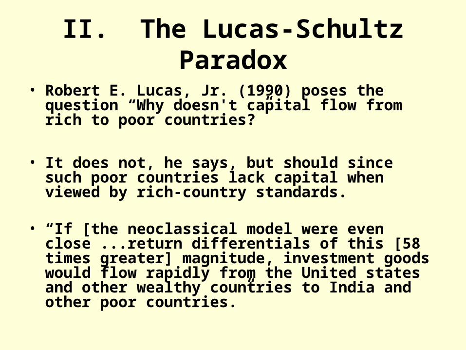
• Robert E. Lucas, Jr. (1990) poses the question “Why doesn't capital flow from rich to poor countries?”

• It does not, he says, but should since such poor countries lack capital when viewed by rich-country standards.

• “If [the neoclassical model were even close ...return

differentials of this [58 times greater] magnitude, investment goods would flow rapidly from the United states and other wealthy countries to India and other poor countries.”

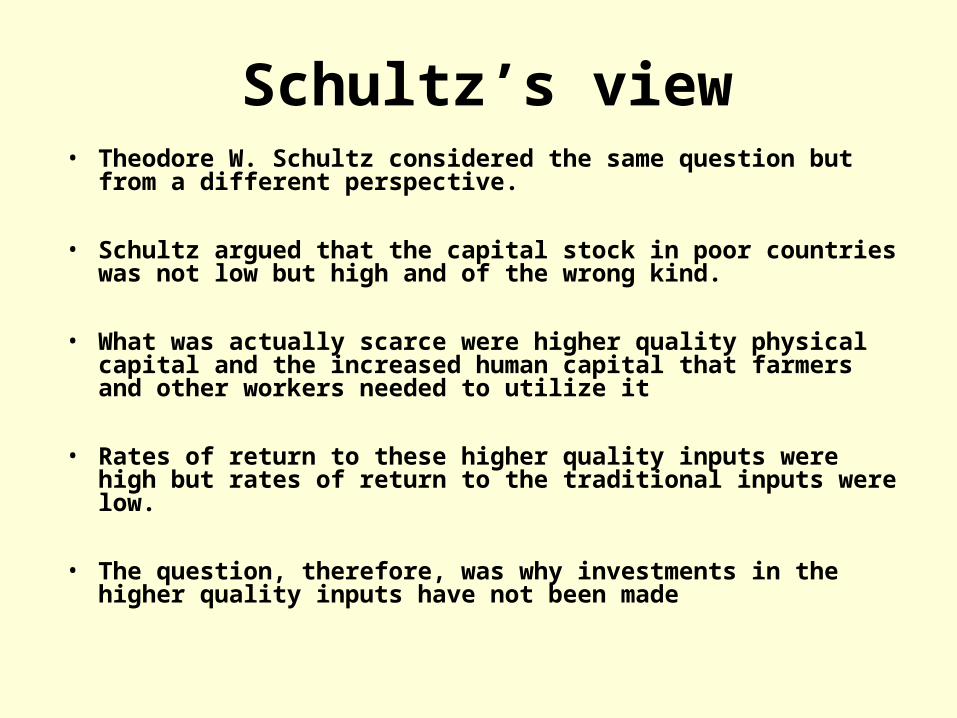
Schultz’s view• Theodore W. Schultz considered the same question but from a

different perspective.

• Schultz argued that the capital stock in poor countries was not low but high and of the wrong kind.

• What was actually scarce were higher quality physical capital and the increased human capital that farmers and other workers needed to utilize it

• Rates of return to these higher quality inputs were high but rates of return to the traditional inputs were low.

• The question, therefore, was why investments in the higher quality inputs have not been made

III. Capital Market Integration in Historical Perspective

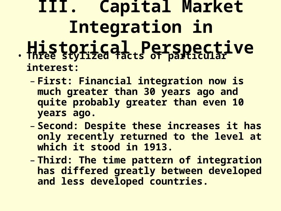
• Three stylized facts of particular interest: – First: Financial integration now is much

greater than 30 years ago and quite probably greater than even 10 years ago.

– Second: Despite these increases it has only recently returned to the level at which it stood in 1913.

– Third: The time pattern of integration has differed greatly between developed and less developed countries.

Real interest rates historically

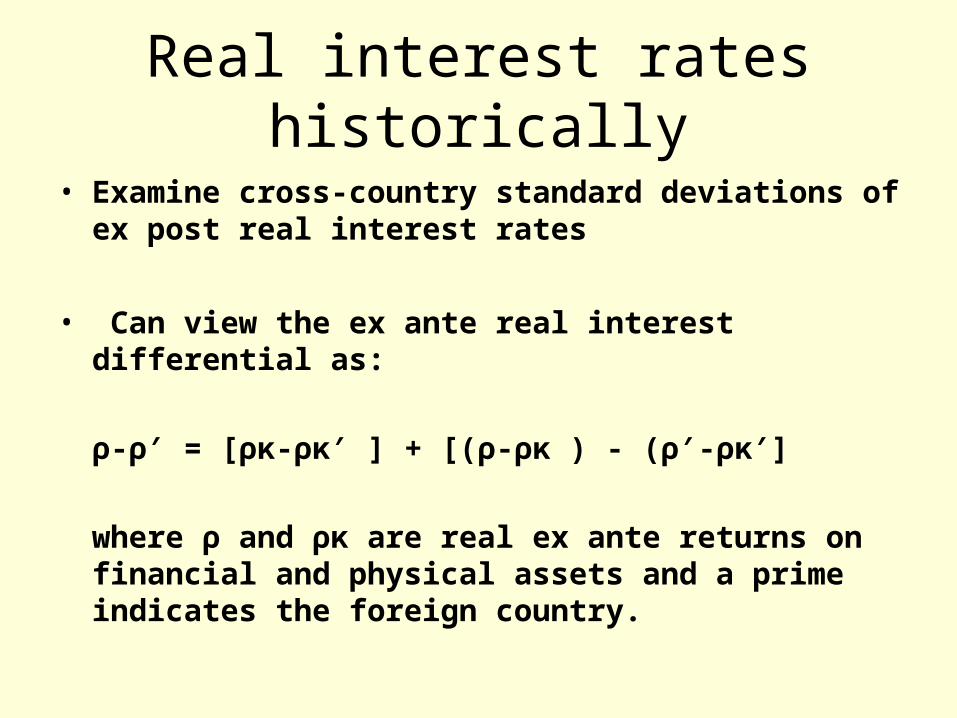
• Examine cross-country standard deviations of ex post real interest rates

• Can view the ex ante real interest differential as:

ρ-ρ′ = [ρκ-ρκ′ ] + [(ρ-ρκ ) - (ρ′-ρκ′]

where ρ and ρκ are real ex ante returns on financial and physical assets and a prime indicates the foreign country.

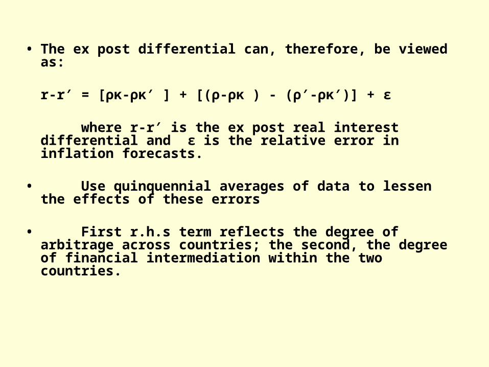
• The ex post differential can, therefore, be viewed as:

r-r′ = [ρκ-ρκ′ ] + [(ρ-ρκ ) - (ρ′-ρκ′)] + ε

where r-r′ is the ex post real interest differential and ε is the relative error in inflation forecasts.

• Use quinquennial averages of data to lessen the effects of these errors

• First r.h.s term reflects the degree of arbitrage across countries; the second, the degree of financial intermediation within the two countries.

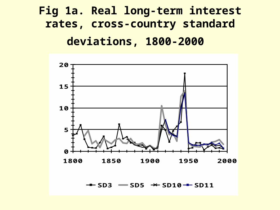
Fig 1a. Real long-term interest rates, cross-

country standard deviations, 1800-2000

0

5

10

15

20

1800 1850 1900 1950 2000

SD3 SD5 SD10 SD11

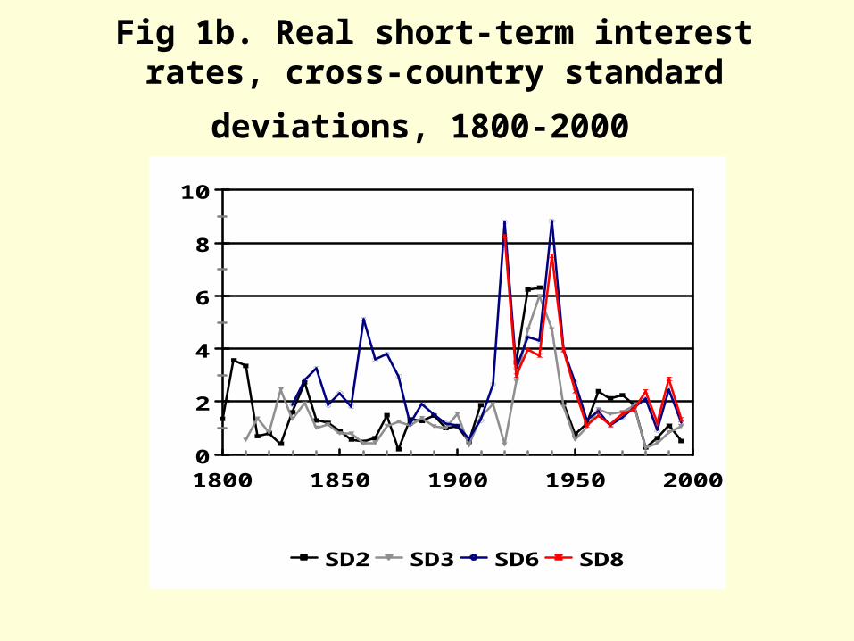
Fig 1b. Real short-term interest rates, cross-

country standard deviations, 1800-2000

0

2

4

6

8

10

1800 1850 1900 1950 2000

SD2 SD3 SD6 SD8

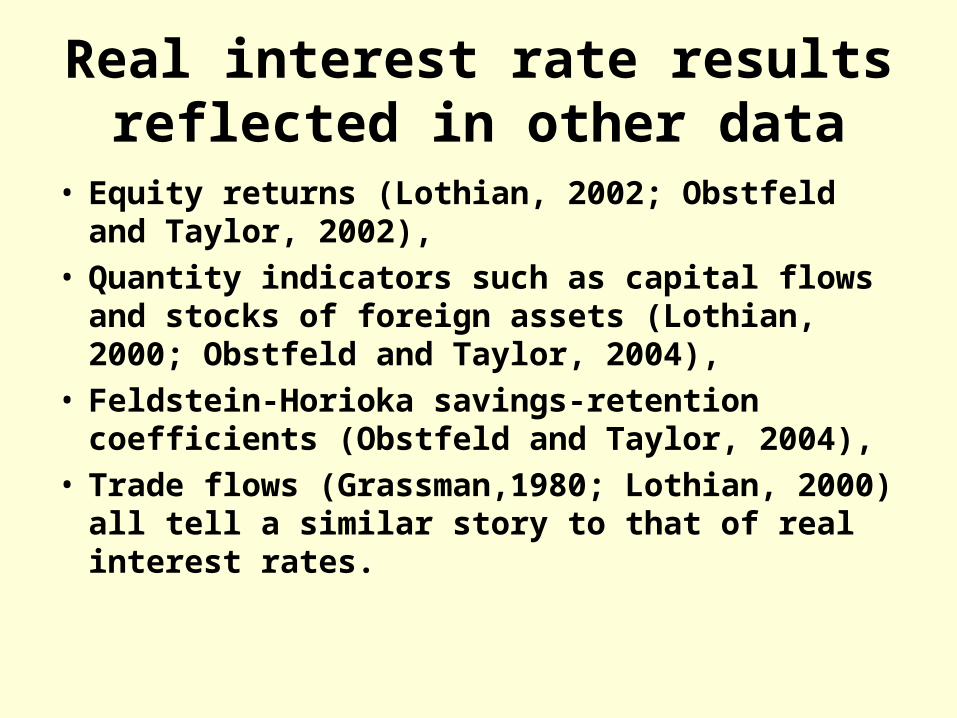
Real interest rate results reflected in other data

• Equity returns (Lothian, 2002; Obstfeld and Taylor, 2002),

• Quantity indicators such as capital flows and stocks of foreign assets (Lothian, 2000; Obstfeld and Taylor, 2004),

• Feldstein-Horioka savings-retention coefficients (Obstfeld and Taylor, 2004),

• Trade flows (Grassman,1980; Lothian, 2000) all tell a similar story to that of real interest rates.

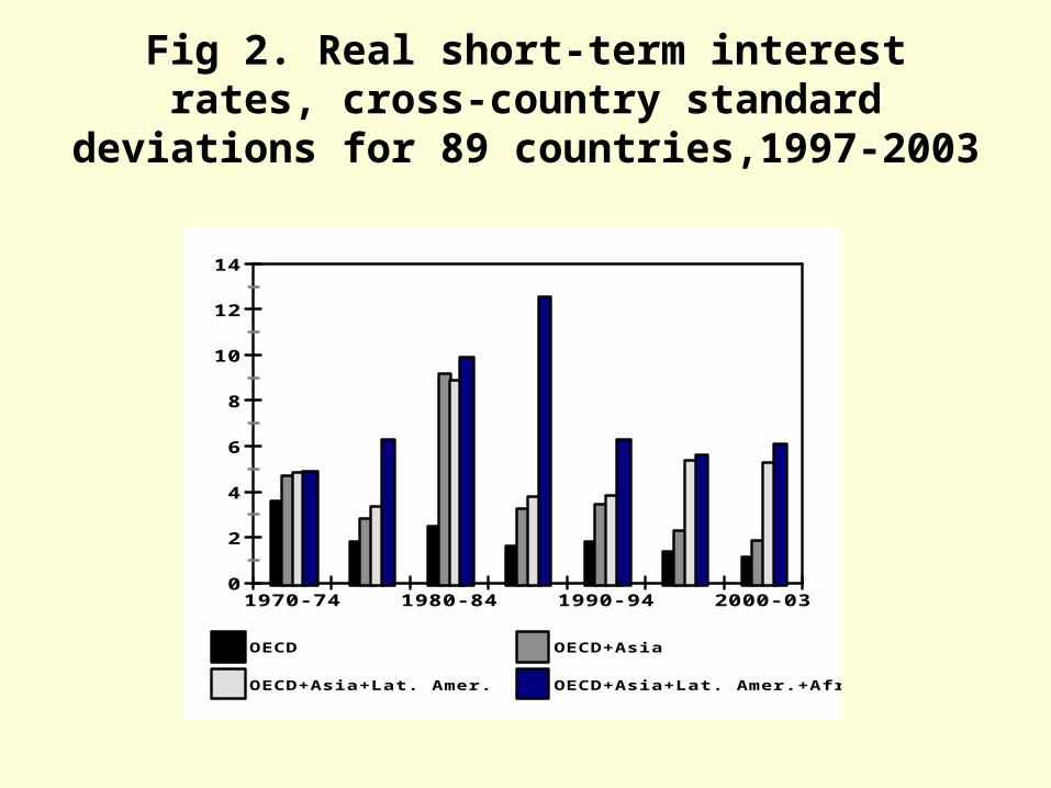
Fig 2. Real short-term interest rates, cross-country standard deviations for 89

countries,1997-2003

0

2

4

6

8

10

12

14

1970-74 1980-84 1990-94 2000-03

OECD OECD+Asia

OECD+Asia+Lat. Amer. OECD+Asia+Lat. Amer.+Africa

The expanded data set

• Three features of the chart stand out:

– Increased cross-country divergences as the three non-OECD groups are added sequentially

– Declines for the OECD and for OECD plus Asia during the last decade and a half

– Progressive narrowing of real-interest rate divergences in the case of OECD versus Asia and the lack thereof for the OECD versus the other two groups.

• Integration therefore much less complete for the periphery vis-à-vis the OECD core, but increasing for Asia, and perhaps some of Latin America-Caribbean, but not for Africa.

Poor countries: Now and Then

• Quantity data tell very much the same story with regard to recent years as the real-interest data.

• In 1997, 82 % of foreign capital investment stocks were in countries with levels of income that were 60% or greater that of U.S. and only 14% in countries with income levels 40% or less that of U.S.

• Situation however was much different a century ago

• In 1913, countries with incomes 40% or less that of the U.S. had a 50% share of the total and countries with income 60% or more that of the U.S. had a 46% share.

Fig. 3a. Distribution of shares of world stock offoreign investment capital by level of receiving country

income per capita (US=100)

0%

10%

20%

30%

40%

50%

<20 20–40 40–60 60–80 >80

Per capita income range of receiving region (U.S.=100)

Sh

are o

f w

orld

sto

ck

of

foreig

n c

ap

ita

l

1913, gross stocks

1997, gross stocks

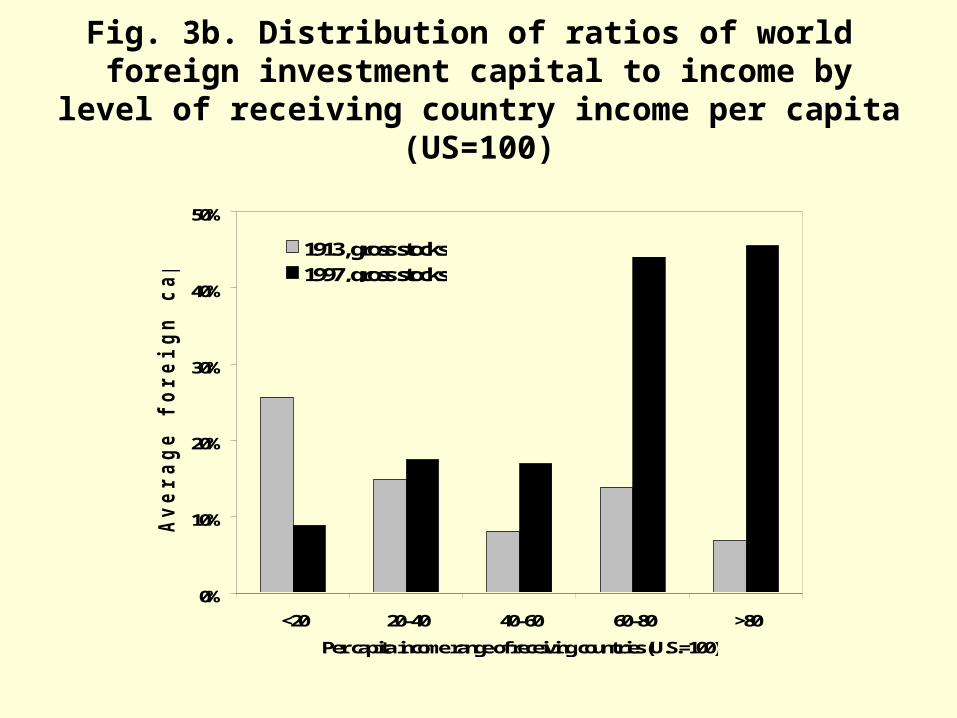
Fig. 3b. Distribution of ratios of world foreign investment capital to income by level of receiving country income per capita (US=100)

0%

10%

20%

30%

40%

50%

<20 20–40 40–60 60–80 >80

Per capita income range of receiving countries (U.S.=100)

Av

era

ge f

oreig

n c

ap

ita

l to

GD

P r

ati

o

1913, gross stocks

1997, gross stocks

IV. Economic Growth and the Lucas-Schultz Paradox

• Closely related to the question of why capital does not flow from rich to poor countries is the question of why poor countries do not grow much more rapidly.

• In the neoclassical model, capital flows to equate real returns and real-income convergence are two aspects of the same process.

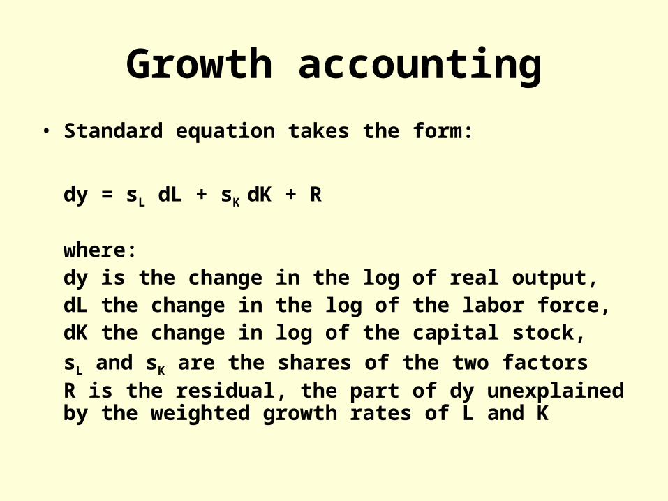
Growth accounting

• Standard equation takes the form:

dy = sL dL + sK dK + R

where:dy is the change in the log of real output, dL the change in the log of the labor force,dK the change in log of the capital stock,

sL and sK are the shares of the two factors R is the residual, the part of dy unexplained by the weighted growth rates of L and K

The relative contributionsof K and L

• In most exercises, R is positive and fairly substantial, often exceeding the contribution of one or the other input and at times the contributions of both.

• Terms applied to R: technological change, human capital accumulation and later total factor productivity (TFP).

Schultz, Transforming Traditional Agriculture (1964)

• Technological improvements and human capital accumulation simply different sides of the same coin.

• Both are improvements in the quality of the conventional labor and capital inputs.

• Standard growth models “not designed to consider the differences in levels of the rates of return to incentives to investment and growth.”

• One of the reasons is that “the profitability of new classes of factors of production have been concealed under ‘technical change.’ ”

Harberger in AEA Presidential Address 1998

• Harberger picks up on some of Schultz’s theme.

• Conventional labels for R should be replaced.

• A better way of viewing R was in terms of “real cost reduction” rather than “technical change” or “TFP.”

• Changes the focus from inventions and externalities to microeconomics.

The focus on real cost reductions

• Enables us to peel the onion a step further and ask the next logical set of questions:– What factor or factors typically account for

these real cost reductions?– Why do those factors operate more

strongly during some time periods and in some places than in others?

Harberger: Government policies and societal institutions are key

• Good policies – price stability, an absence of distorting government intervention at the levels of the firm and the household, open international trade and the like – and good institutions, the enforcement of private property being key – enable growth.

• Provide incentive to engage in activities that reduce real costs and also raise the rate of return to investment.

• Bad policies and bad societal institutions have reverse effects.

Policies and institutions

• Impact of institutional factors on growth has been the theme of a much other literature in recent years: North’s (1990), historical treatments, to DeSoto’s (2000) descriptive account of the day-to-day difficulties entrepreneurs faced in developing countries, to econometric investigations of various sorts (e.g., Barro, 1998).

• Recent cross-country study (2004) by Gwartney, Holcombe, and Lawson (GHL) is particularly germane.

The GHL Study

• Major feature of the study is the use of the Economic Freedom of the World Index (EFW)

• EFW index is made up of 5 component indices: size of government, legal system and property rights, sound money, freedom to trade internationally, and regulation, each of which, in turn, has anywhere from 3 to 18 components.

• GHL use the EFW index as a regressor in cross-country regressions along with other variables common in the growth literature as controls to investigate the impact of policies and institutions on both on the level of real per capita GDP and its rate of growth.

• GHL report statistically significant and economically meaningful EFW effects in all instances.

• Find largely similar effects for the per-worker stocks of physical and human capital, the rates of change of both and the ratios of investment and foreign direct investment to GDP.

• Rerun real GDP growth regressions using residuals from these latter regressions in place of the actual variables as regressors.

• Allowing for both direct and indirect EFW effects in this way increases the estimated EFW impact substantially.

V. Policies, Institutions and Capital Flows

• I extend the GHL approach is to capital flows

• Use the EFW index and data from Lane and Milesi-Ferretti (2001) and the World Bank’s Global Development Finance data base.

• Find substantial differences in flows across countries grouped by level of EFW index and statistically significant relationships

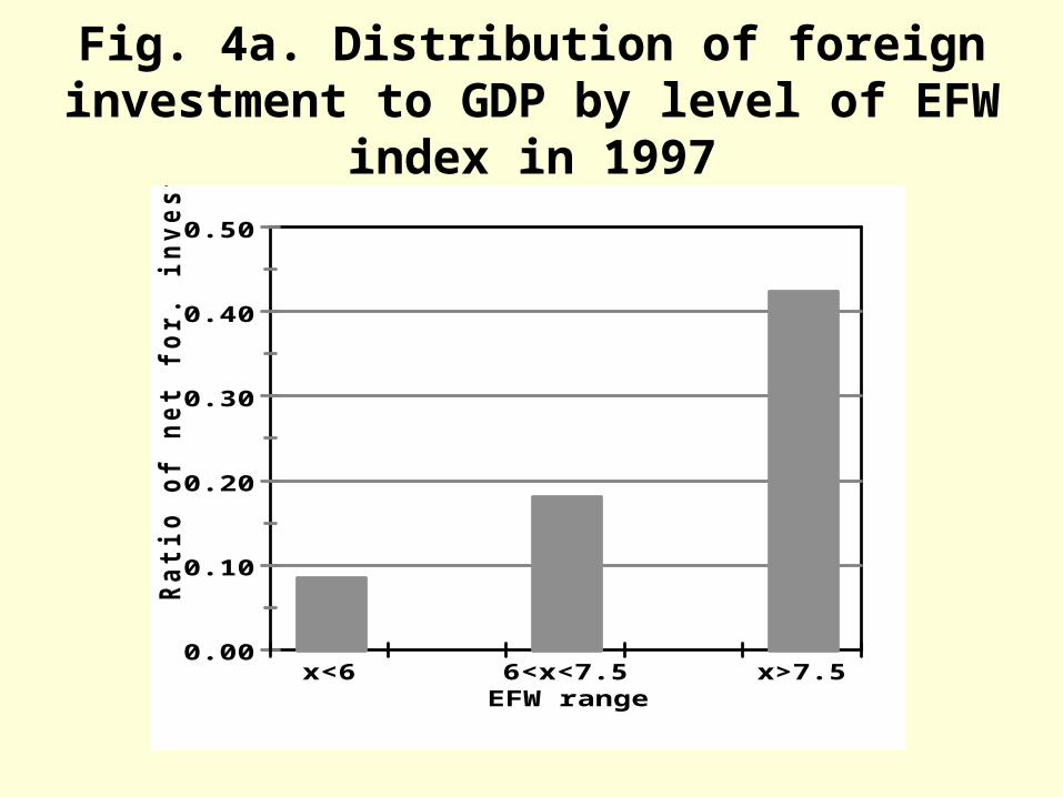
Fig. 4a. Distribution of foreign investment to GDP by level of EFW index in 1997

0.00

0.10

0.20

0.30

0.40

0.50

Rati

o o

f n

et

for.

in

vest.

to

GD

P

x<6 6<x<7.5 x>7.5EFW range

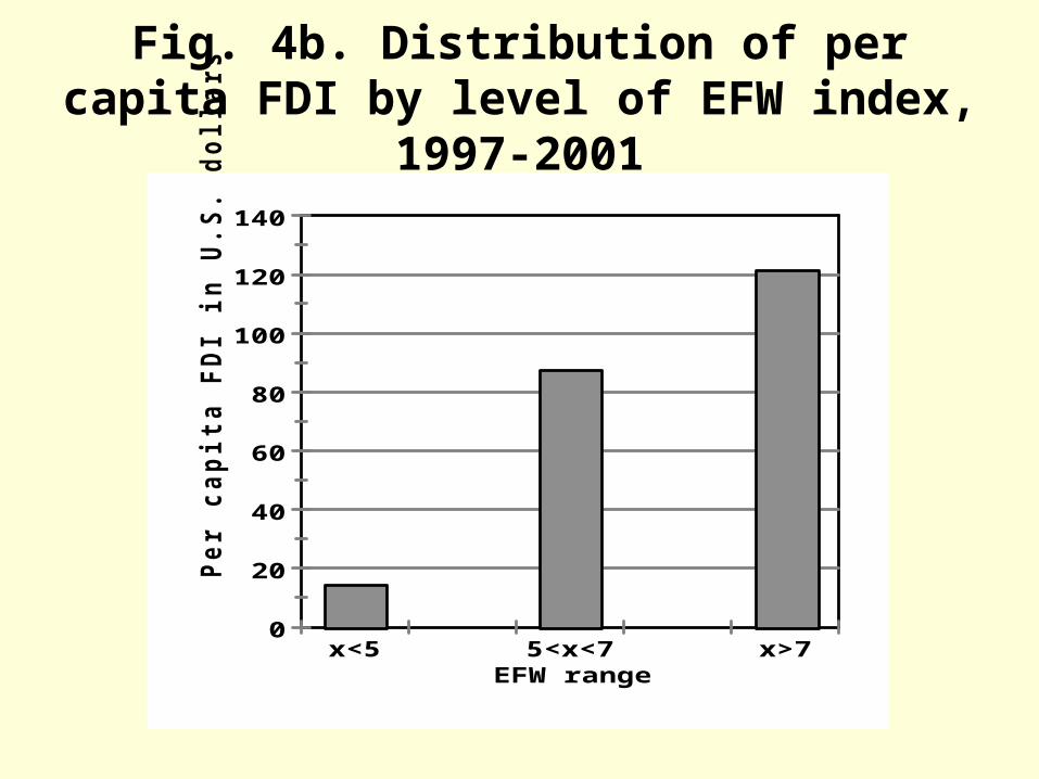
Fig. 4b. Distribution of per capita FDI by level of EFW index, 1997-2001

0

20

40

60

80

100

120

140P

er

cap

ita F

DI in

U.S

. d

ollars

x<5 5<x<7 x>7EFW range

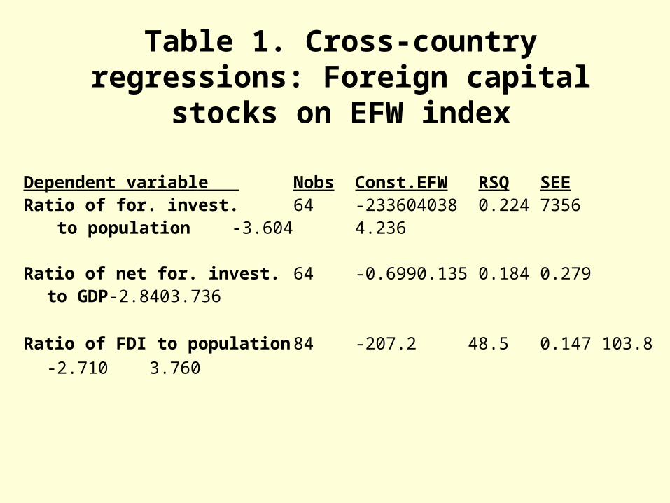
Table 1. Cross-country regressions: Foreign capital stocks on EFW index

Dependent variable Nobs Const. EFW RSQ SEERatio of for. invest. 64 -23360 4038 0.224 7356

to population -3.604 4.236

Ratio of net for. invest. 64 -0.699 0.135 0.184 0.279to GDP -2.840 3.736

Ratio of FDI to population 84 -207.2 48.5 0.147 103.8

-2.710 3.760

VI. Conclusions• Let’s return to the question with which we started –

why capital flows to poor countries remain so sparse.

• Savers in rich countries, it seems, should be taking much greater advantage of the high returns that in principle should await them as they did a century ago.

• I have argued that the reason it is not happening now is due to the institutions that are in place and the policies that have been pursued in many if not most poor countries

• In this regard, the emerging market countries are, I believe, the exception that proves the rule.