Title Institutions and corporate investment: Evidence frominvestment-implied return on capital in China

Author(s) Liu, Q; Siu, A

Citation Journal Of Financial And Quantitative Analysis, 2011, v. 46 n. 6,p. 1831-1863

Issued Date 2011

URL http://hdl.handle.net/10722/152924

Rights This work is licensed under a Creative Commons Attribution-NonCommercial-NoDerivatives 4.0 International License.

Institutions and Corporate Investment: Evidence from

Investment-Implied Return on Capital in China∗

Qiao Liu †

University of Hong KongAlan Siu ‡

University of Hong Kong

This Draft: September 2010

Abstract

We assess the impact of institutions on Chinese firms’ corporate investment in aninvestment Euler equation framework. We allow the variables measuring institutionsto affect the rate at which firm managers discount future investment payoffs. Applyinggeneralized method of moments estimators to large samples of Chinese firms, weestimate the stochastic discount rates derived from actual investment and examine howthey vary across institutional variables. We document robust evidence that ownershipis the primary institutional factor affecting corporate investment in China. The deriveddiscount rate for a non-state firm is approximately 10 percentage points higher thanthat of an otherwise equal state firm. State firms tend to use higher discount rates toinvest after they are partially privatized. We also find that firms with higher levels ofcorporate governance use higher discount rates to make investment.

JEL Classification: G31; G34; G18; D21; O16Keywords: Institutions, investment Euler equation, investment-implied discount rate,corporate governance, Chinese economy

∗We are grateful to an anonymous referee for many constructive suggestions that have greatly improvedthe paper. We thank Toni Whited for kindly sharing programming codes and offering computationsuggestions. We also thank Hongbin Cai, Joseph Fan, Qiang Kang, Hongbin Li, Wing Suen, Chenggang Xu,Charles Leung, Yong Wang, Guofu Zhou, and seminar participants at Keio University, Beijing University,University of Hong Kong, Chinese University of Hong Kong, City University of Hong Kong, TsinghuaUniversity, the Central University of Finance and Economics, and the 2007 China International Conferencein Finance (CICF) for useful comments, and Yong Wei for able research assistance. Financial support fromthe University Grants Committee of the Hong Kong Special Administrative Region, China (Projects No.AOE/H-05/99, HKU7472/06H, and HKU747107H) are gratefully acknowledged. All errors remain our ownresponsibility.†Corresponding author. School of Economics and Finance, University of Hong Kong, Hong Kong.

Phone: (852) 2859 1059. Fax: (852) 2548 1152. E-mail: qliu@hku.hk.‡School of Economics and Finance, University of Hong Kong, Hong Kong. Phone: (852) 2857 8505. Fax:

(852) 2548 1152. E-mail: asiu@econ.hku.hk.

Institutions and Corporate Investment: Evidence from Investment-Implied

Return on Capital in China

Abstract

We assess the impact of institutions on Chinese firms’ corporate investment in an

investment Euler equation framework. We allow the variables measuring institutions

to affect the rate at which firm managers discount future investment payoffs. Applying

generalized method of moments estimators to large samples of Chinese firms, we

estimate the stochastic discount rates derived from actual investment and examine how

they vary across institutional variables. We document robust evidence that ownership

is the primary institutional factor affecting corporate investment in China. The derived

discount rate for a non-state firm is approximately 10 percentage points higher than

that of an otherwise equal state firm. State firms tend to use higher discount rates to

invest after they are partially privatized. We also find that firms with higher levels of

corporate governance use higher discount rates to make investment.

JEL Classification: G31; G34; G18; D21; O16

Keywords: Institutions, investment Euler equation, investment-implied discount rate,

corporate governance, Chinese economy

1 Introduction

A large and growing literature investigates the effects of institutions on economic performance

and finds that good institutions promote economic development.1 Much of this literature

is based on cross-country studies that are likely subject to contamination due to country

differences in accounting standards, taxation, and bankruptcy laws. This literature also fails

to account for obvious outliers such as China — the unprecedented economic growth over

the past three decades in China has been based largely on weak institutions and inefficient

financial intermediation (Allen, Qian and Qian, 2005). In this paper, we use an investment

Euler equation framework to examine the extent to which institutions affect Chinese firms’

investment behavior. Applying generalized method of moments (GMM) estimators to large

samples of Chinese industrial firms, we estimate the rates these firms use to discount future

investment payoffs. We then examine how this investment-implied return on capital or

discount rate varies across variables measuring institutions. We document robust evidence

that ownership is the primary institutional factor affecting firm-level return on capital in

China. The investment-implied return on capital for a non-state firm is approximately 10

percentage points higher than that of an otherwise equal state firm. We also find that state

firms use higher discount rates to invest after they are partially privatized and that firms

with better corporate governance have a higher return on capital.

The motivations for our inquiry are three fold. First, there is little empirical evidence

at the micro level on the dynamic relation between corporate investment and institutions.

For instance, while heavy investment and exports have long been viewed as two pillars of

China’s economic ascendancy, few studies examine how institutional factors shape Chinese

firms’ investment behavior. We contribute to this line of research by presenting evidence from

large samples of Chinese industrial firms. Second, extant studies rely largely on cross-country

analysis and reduced-form regressions. Drawing clean inferences from these studies might be

1See, e.g., Acemoglu, Johnson and Robinson, 2001; Claessens and Laeven, 2003; Levine and Zervos, 1998;Rajan and Zingales, 1998; and Bekaert, Harvey, and Lundblad, 2005.

1

difficult as they are unavoidably plagued by endogeneity. By estimating a structural model of

corporate investment, we potentially mitigate this concern. Third, in our structural setting,

the effects of institutions on corporate investment are readily captured by the stochastic

discount rates inferred from actual corporate investment. This investment-implied return on

capital reveals firm managers’ true propensity to investment and can be interpreted in an

intuitive way. In addition, our approach is not restricted to publicly listed firms, and imposes

minimal requirements on capital market information, and thus may be useful for research

on emerging markets, where capital markets are under-developed and financial disclosure is

limited and less transparent.

We begin by constructing a standard intertemporal investment model that characterizes

the investment allocation of a utility-maximizing firm manager. The manager maximizes

utility by choosing how much income to consume and how much income to invest in each

period. Dividend consumption is constrained by the firm’s profit function and the manager’s

investment decision. The manager chooses the optimal level of investment so as to be

indifferent between investing today and investing tomorrow. The model produces results

in terms of intertemporal investment substitution where the stochastic discount factor is

related to the manager’s risk preference — a lower discount factor (a higher discount rate)

corresponds to a more cautious attitude toward corporate investment. The model allows

firm managers’ discount rates to vary across variables measuring institutions. The effects of

institutions on corporate investment are thus captured by the differences in discount rates

that firm managers use to make investment decisions.

The intuition for using an investment Euler equation to assess the effect of institutions on

corporate investment is easiest to see in a simple two-period example. When a firm manager

considers investing today versus tomorrow, he has to consider the costs and benefits of

this decision. Investing today entails a cost today whereas investing tomorrow defers the

cost until later and thus reduces this cost in terms of its present value. However, investing

tomorrow entails forgoing the marginal product of capital for one period. An investment

2

Euler equation is simply a first-order condition that equates the marginal cost of investing

today and the expected discounted cost of investing tomorrow. In this setting, the discount

rate characterizes the manager’s willingness to invest. If the manager becomes more cautious

or less willing to embark on new and risky projects, this increased caution will be reflected

as an increase in the discount rate.

We expect that all else being equal, the discount rates used by managers of state owned

enterprises (SOEs hereafter) to discount future investment payoffs are lower than those

used by managers of other types of firms. Denoting the discount rate for an SOE as rSOE

and the discount rate for other types of firms as r, we conjecture that r = rSOE + θ. In

the Chinese context, θ is likely to be greater than 0 for two reasons. First, due to their

soft budget constraints, SOEs are afflicted with an “investment hunger” problem (see, e.g.,

Kornai, 1980); they demonstrate stronger preference for investment, and adopt relatively

lower discount rates. Over-investment is thus more likely to be a concern among SOEs.

Second, non-state firms, especially private firms, are exposed to a variety of institutional

constraints (e.g., policy and tax distortions and expropriation by the government), and

hence may be more cautious about investment.

Notably, a positive θ may also result from a high level of financing constraints facing

non-state firms simply because these firms are not favored by the state-dominated financial

system. Institutional deficiencies and financing constraints interact to affect corporate

investment in China. While our empirical strategy centers on exploring the magnitude

and distribution of θ, it cannot disentangle the impact of external financing constraints from

that of institutions. However, we believe that a positive θ is mainly driven by institutional

deficiencies for three reasons. First, asymmetric access to finance is itself a reflection of

poor institutions (i.e., lack of a level playing ground). Second, when we compare SOEs to

mixed-ownership firms, the majority of which are former SOEs that are still controlled by

the state, we find that while the mixed firms display no significant difference in their access

3

to external finance, their θ is significantly positive.2 Third, we find similar results when we

apply the same approach to the privatized SOEs and the listed firms in China, which are

less subject to external financing constraints.

Our empirical analysis formalizes the above intuition. The Euler equation governs the

manager’s decision on how much to invest. The Markovian nature of our model reduces

the manager’s infinite-horizon dynamic problem to an optimality condition concerning

investment this period versus next period. The effects of institutions on corporate investment

are captured by θ, which is closely related to institutional variables such as ownership. It is

possible to identify these effects from the cross-sectional variation in corporate investment.

Further, after controlling for a measure of investment opportunity (i.e., capital productivity),

we can identify whether cross-sectional variation in investment is caused by differences in

the stochastic discount rate or differences in productivity, which alleviates the endogeneity

concern that arises in a reduced-form regression framework. We interpret higher discount

rates among well-governed firms as evidence that good institutions mitigate over-investment.

Alternatively, one may argue that imposing higher discount rates may delay or deter valuable

investments, potentially causing under-investment. While we cannot completely rule out this

possibility, we believe that it is less a concern. Throughout our empirical analysis, we control

for investment opportunities and other firm-specific variables, and thus systematic differences

in discount rates most likely reflect the effects of institutions. Moreover, given that over-

investment and in turn over-capacity have been the primary structural problems challenging

the Chinese economy, little anecdotal and empirical evidence shows that under-investment

is a pervasive concern in the absence of external financing constraints.

We estimate our investment Euler equation using generalized method of moments (GMM)

estimators. A key advantage of this approach is that it avoids sample selection, simultaneity,

and measurement error biases via structural estimation with a large dataset. Using actual

2The difference between SOEs’ and other types of firms’ discount rates, θ, may also capture the effects offactors other than institutional deficiencies on corporate investment, e.g., irrational decision making by firmmanagers, etc. However, these factors are likely to be firm-specific and their effects likely average out whenaggregating.

4

corporate investment data retrieved from a well-maintained dataset developed by the

National Bureau of Statistics of China (NBS), we apply GMM estimators to a panel of

36,103 industrial firms from 2000 to 2005. We parameterize the stochastic discount factor as

a linear function of variables measuring institutions and firm-specific characteristics. Based

on the estimated structural parameter values, we compute the “implied” return on capital or

discount rate and examine its distribution. The estimates of our model yield several principal

findings. First, we find that the inferred discount rate varies significantly across ownership.

In our benchmark estimation, the inferred return on capital for a private firm, a Hong Kong,

Macao, or Taiwan invested firm (HK/TW firm), a foreign firm, a mixed firm (i.e., joint stock

firm), and a collective firm is respectively 9.4, 11.9. 10, 13, and 11.4 percentage points higher

than that of an otherwise equal SOE. Second, we find that the ownership effect is robust

to controlling or industries and the level of regional institutions and financial development,

indicating that ownership is the primary institutional factor affecting corporate investment

in China.

To shed further light on the effects of institutions on corporate investment, we apply the

same GMM estimators to another two samples of Chinese firms, the SOEs that were partially

privatized during our sample period and the universe of Chinese listed firms. Firms in these

two samples are less subject to external financing constraints and a positive θ is more likely

to be driven by institutions rather than financing constraints. Our GMM estimations on the

two samples yield very similar results. In particular, we find that an SOE tends to use a

higher discount rate to invest after it has changed its ownership status from SOE to mixed.

We also find that all else being equal, a state-control listed firm has an implied return on

capital that is 15.8 percentage points lower than that of an otherwise equal listed firm. In

addition, we provide evidence that firms with a larger fraction of outside board members,

firms with more shares held by a controlling shareholder, and firms with H– or B– shares

traded by foreign investors have a higher return on capital. Well-governed firms in China

are more cautious about investment and are less subject to the over-investment problem.

5

Overall, we contribute to the literature on corporate investment and institutions.

Different from Dwenter and Malatesta (2001), Love (2003), and Wurgler (2000), we focus

on a single country and use more detailed firm-level data, which allows us to construct a

richer set of variables in examining the factors affecting corporate investment and to better

control for potential contamination due to cross-country differences. Moreover, we study the

case of China, which is of particular interest not only because of its size, but also because

it is an obvious outlier in most cross-country studies on the relation between institutions

and economic performance. While fixed asset investment remains one of the most significant

pillars of China’s economic growth, little research examines corporate investment and the

underlying economic and institutional factors that shape corporate investment behavior.

Deriving firm level returns on capital from actual capital expenditures and mapping out

their various cross-sections help us better understand corporate investment in China.

We also contribute to a small but growing literature on investment efficiency and resource

mis-allocation in China. Bai, Hsieh, and Qian (2006) use aggregate data to estimate return

to capital in China. However, using aggregate data cannot directly measure the extent of

capital mis-allocation and link corporate investment behavior to institutional factors. Hsieh

and Klenow (2007) provide evidence of sizable gaps in the returns to capital across firms

within the same sectors in China and India compared to the U.S. But they do not investigate

systematically how the mis-allocation of capital is related to institutions. Dollar and Wei

(2007) examine how institutions such as ownership and regional economic development affect

corporate investment efficiency. But they use reduced-form model specifications based on

a small sample of survey data, and their measure of investment efficiency — the observed

average revenue product of capital — captures operating performance rather than ex ante

managerial investment propensity. Moreover, to argue that institutions enhance investment

efficiency at the micro level requires identifying firms that “should” be growing given their

investment opportunities.

We additionally contribute to the investment Euler equation literature (see, e.g.,

6

Whited, 1992; Forbes, 2007; Love, 2003; Chirinko and Schaller, 2004; and Whited and

Wu, 2006) and to the investment-based asset pricing literature, which explains the cross-

section of expected stock returns or costs of equity from the perspective of value-maximizing

firms (see, e.g., Cochrane, 1991; Zhang, 2005; and Liu, Whited, and Zhang, 2009). Liu,

Whited, and Zhang (2009) use investment Euler equations to derive cross-sectional expected

stock returns, which are essentially levered investment returns tied to firm characteristics.

Our use of investment Euler equations focuses instead on the effects of institutional variables

on corporate investment via the discount rates perceived by firm managers. Our paper thus

is similar in spirit to Kang, Liu, and Qi (2010), who apply an investment Euler equation

framework to examine how government regulations (the Sarbanes-Oxley Act) affect firm

investment in the U.S.

The rest of the paper proceeds as follows. Section 2 discusses the institutional background

in China and related literature, and presents four hypotheses on the potential effects of

China-specific institutions on corporate investment. Section 3 provides an investment model

and describes our estimation strategy. Section 4 discusses the data and variables used in our

empirical analysis. In Section 5, we discuss the effect of ownership on corporate investment,

and in Section 6 we estimate our model for the privatized SOEs and the Chinese listed firms,

respectively. Finally, we conclude the paper in Section 7.

2 Institutional Background and Corporate Investment

in China

China’s striking economic growth over the past three decades has been driven largely by

fixed asset investment. As evidenced by the most recent global economic crisis, when China’s

exports experienced a significant drop as a result of weak demand in the developed economies,

investment became the single most important pillar to sustain China’s growth. Two distinct

features characterize fixed asset investment during China’s reform era. First, the rate of

7

fixed asset investment has hovered at a high level, partly due to a high domestic savings

ratio and China’s success in attracting foreign direct investment (FDI). As shown in Table

A1, fixed asset investment accounts for nearly 50% of China’s GDP, which from time to time

raises the concern that the Chinese economy is overheating due to over-investment. Second,

as shown in Table A2, more than 50% of fixed asset investment concentrates in the state

sector or the quasi-state sector, where productivity and investment efficiency are believed to

be considerably low.

The excessive amount of capital allocated to the state sector results in widespread

inefficiency among SOEs, reduced overall productivity of the economy, and a large amount

of non-performing loans.3 Prior literature has identified several sources of inefficiency in

corporate investment, and attributes these sources to insufficient or weak institutions and

inefficient financial intermediation. First, during the reform era, China can be described

as a de facto federalism, with local governments having significant autonomy in economic

matters (Qian and Xu, 1993). Local bureaucrats are assessed and promoted primarily based

on local economic growth driven by investment. Returns generated by investment help pay

for social spending on everything from education to health care — costs that are now the

local governments’ responsibility. Local officials therefore have strong incentives to approve

new projects to stimulate economic growth. A large number of such investments have been

labeled “image” projects (projects undertaken by local governments to boost their local

image) or “political achievement” projects (projects undertaken to boost local bureaucrats’

scores on key performance indicators), and inherently suffer from dim earnings prospects.

From time to time, the central government has to take a slew of measures such as raising

bank lending rate and/or bank reserve requirements, and sometimes outright administrative

methods to put the brakes on investment boom to ensure that overheated investment does

not lead to inflation and a pile-up of bad loans.4

3As Farrell et al. (2006) show, during the first half of the 1990s, $3.30 of investment was needed to produce$1.00 of GDP growth in China. Since 2001, $1.00 of GDP growth has required $4.90 of new investment —40% higher than the amount required in South Korea and Japan during their higher-growth periods.

4One recent example occurred in August 2006, when the governor of Inner Mongolia and his two

8

Second, the state-dominated financial system in China has systematically allocated

capital away from more productive sectors/regions toward less effective sectors/regions (see,

e.g., Young, 2001; Brandt and Li, 2003; Cull and Xu, 2003; and Boyreau-Debray and

Wei, 2005). Because of their soft budget constraints, SOEs are afflicted with a pervasive

“investment hunger” problem and are prone to over-investing regardless of the demand for

their products (Kornai, 1980). Legally and financially, inefficient SOEs are favored at the

expense of more efficient non-state sectors (Huang, 2003).

Despite numerous anecdotes and sound economic intuition, it remains empirically difficult

to map out the dynamic relation between corporate investment and institutions. In this paper

we propose a new empirical approach and provide direct evidence on Chinese firms’ corporate

investment. Using actual corporate investment data, we estimate investment Euler equations

that characterize Chinese firms’ investment behavior to derive the effective discount rate

perceived by firm managers in making investment spending decisions. This implied return

on capital is similar to the managerial hurdle rate, and is potentially a function of variables

measuring institutions.

The soft budget constraints afflicting SOEs and the fact that local governments act as

decision makers suggest that SOEs may demonstrate stronger investment propensity and

hence adopt lower discount rates: SOEs are favored by the state (e.g., they are less subject

to regulatory burdens, insecure property rights, and credit constraints), and thus they are

likely to perceive lower costs of capital. Non-state sectors, in contrast, are exposed to a

variety of institutional constraints, and are more likely to adopt higher hurdle rates to make

investment. Using the notation introduced earlier, we therefore argue that rSOE is a distorted

reflection of the market price of capital, in particular, it tends to be lower than the market

rate, and that the gap between rSOE and r is likely to be positive and persistent. We thus

lieutenants were publicly criticized by the State Council for disobeying the central government’s call toslow investment by allowing hundreds of millions of dollars of investment in coal-burning power plants.This investment boosted local economic growth but has been associated with ever-worsening environmentalproblems in the northern part of China, several fatal accidents, and low efficiency (source: the Wall StreetJournal - Asia Edition, August 18, 2006).

9

have the following hypothesis:

H1: The implied return on capital derived from actual investment is lower for SOEs and

higher for non-state firms (i.e., collective firms, private firms, HK/TW firms, and foreign

firms.)

We next conjecture that product market competition affects corporate investment

behavior as well. Intuitively, firms in a more competitive market likely face greater pressure

from their rivals and hence are more cautious in making investment decisions. The impact

of competition on corporate investment could be much more involved, however. Taking into

account the fact that firms’ options exercise strategies are formed strategically as part of a

Nash equilibrium (i.e., are not formulated in isolation), several studies (e.g., Grenadier, 1996,

2002; and Williams, 1993) show that an increase in competition leads to earlier exercise of

options. In the context of real-world corporate investment, the playing of a strategic exercise

game implies that an increase in competition may actually speed up investment.5 We thus

expect a negative effect of competition on discount rates.

In addition, given significant cross-regional variation in the quality of institutions, we

expect the implied return on capital to be higher for firms located in regions with better

institutions and a more market-oriented financial system.6 Combining the competition and

regional institution factors, we have:

H2: The implied return on capital derived from actual investment is higher for firms operating

in a less competitive market and for firms located in regions with better institutions and a

more market-oriented financial system.

Note that a caution has to be taken here because both competition and regional

institutions are highly correlated with the presence of state ownership. Their effects on

implied return on capital may therefore be camouflaged by the ownership effect.

5We are grateful to an anonymous referee for pointing out this explanation and its ensuing insight.6Using Italian data, Guiso, Sapiegza, and Zingales (2004) document that local financial development

enhances the probability that an individual starts his own business, favors entry of new firms, increasescompetition, and promotes growth. Local financial development is an important determinant of the economicsuccess of an area.

10

If institutions affect corporate investment, firms’ investment decisions should be different

once the institutions concerning firms have been improved. The on-going privatization wave

in China provides us with an opportunity to examine how changes in institutions affect

corporate investment decisions. Converting SOEs to joint stock companies (i.e., mixed-

ownership companies) has been the common privatization route in China. The conversion

may takes many forms. Selling part of the shares to non-state shareholders and even the

public via initial public offerings (IPOs) is the common practice. We conjecture that an

SOE’s investment will be improved after it changes its ownership status from SOE to mixed.

We have:

H3: The SOEs’ implied return on capital increases after they have been partially privatized.

While we argue that the sign and magnitude of θ capture differences in corporate

investment caused by institutional deficiencies, a positive θ may also result from a high

level of financing constraints faced by non-state firms simply because these firms are not

favored by the state-dominated financial system. Testing H3 above may help to disentangle

the impact of external financing constraints from the impact of institutions because the

majority of privatized SOEs are still state controlled.

In the same vein, we apply the same estimators to the universe of China’s listed firms,

among which external financing constraints are less severe. We expect that all else being

equal, firms with better corporate governance tend to be more cautious about investment.

Evidence from the sample of Chinese listed firms should more likely reflect differences in

corporate investment behavior caused by institutions. We have:

H4: All else being equal, the implied return on capital is higher for firms with better corporate

governance.

11

3 Model and Estimation Strategy

To motivate our empirical work and provide guidance on the choice of control variables in the

estimation, we offer a simple partial-equilibrium model in which a firm manager maximizes

expected utility by choosing investment and consumption. We derive our investment Euler

equation from this simple model. We then outline the framework for our empirical analysis.

3.1 A Simple Model

Consider an infinitely lived firm i that uses capital to produce goods in each period t. The

firm manager maximizes the expected present discounted value of his utility over an infinite

horizon,

Vi0 = Ei0

[∞∑t

βu(dit)

], (1)

where Ei0 is the expectations operator conditional on the manager’s time 0 information set;

β is the one-period discount factor common to all firms; u(.) is the manager’s utility function

(if the manager is risk-averse, the utility function is concave); and dit is the dividend paid

by firm i in period t.

The manager maximizes Equation (1) subject to two conditions. The first defines

dividends,

dit = Π(Kit, ζit)− C(Iit, Kit)− Iit, (2)

where Kit is the beginning-of-period capital stock; ζit is a shock to the profit function that

follows a Markov process and is observed by the firm at time t; Π(Kit, ζit) is the firm’s profit

function with ΠK ≡ ∂Π∂K

> 0; Iit is investment during time t; and C(Iit, Kit) is the real cost

of adjusting the capital stock, with ∂C∂I> 0, ∂C

∂K< 0, and ∂2C

∂I2 > 0.

The second condition characterizes capital stock accumulation,

Kit+1 = (1− δi)Kit + Iit, (3)

12

where δi is the firm-specific constant rate of economic depreciation.

The choice variables in this model are Iit and dit, and the state variable is Kit. Solving

the model yields the Euler condition for Kit:

1 + (∂C

∂I)it = Eit

[βu′(dit+1)

u′(dit)

{(∂Π

∂K)it+1 − (

∂C

∂K)it+1 + (1− δi)(1 + (

∂C

∂I)it+1)

}], (4)

where ∂C∂I

is the marginal adjustment cost of investment; β u′(dit+1)u′(dit)

is the marginal rate

of substitution of dividends, or the pricing kernel from a consumption-based asset pricing

model; and ∂Π∂K

is the marginal profit of capital. For notational convenience, we define

Γit+1 ≡ β u′(dit+1)u′(dit)

. We immediately rewrite Equation (4) as follows:

1 + (∂C

∂I)it = Eit

[Γit+1

{(∂Π

∂K)it+1 − (

∂C

∂K)it+1 + (1− δi)(1 + (

∂C

∂I)it+1)

}]. (5)

The Euler equation in Equation (5) describes the evolution of the firm manager’s

investment decisions along the optimal path and has an intuitive interpretation. To decide

whether to invest in the current period versus in the next period, a manager must consider the

costs and benefits of the timing decision. This equation is simply a first-order condition that

describes the optimal intertemporal allocation of investment. The left-hand side represents

the marginal adjustment cost of investing in this period. The right-hand side represents

the expected discounted cost of deferring investment to next period, which consists of

the marginal product of capital and the marginal reduction in adjustment costs from an

increment to the capital stock. Notice that even if the firm waits, it still incurs adjustment

costs. Optimizing investment necessitates that, on the margin, the manager must be

indifferent between investing in the current period and transferring those resources to the

next period.

The factor Γit+1 in Equation (5) merits further discussion. By construction, Γit+1 is

the product of the discount factor common to all firms (β) and the ratio of the marginal

utility of dividends in the next period to the marginal utility of dividends in the current

13

period. Because our investment Euler equation characterizes the optimal intertemporal

allocation of investment, Γit+1 is essentially the discount factor that the firm manager uses

to discount the investment returns in the next period. While Γit+1 is clearly related to the

manager’s preferences, it can be interpreted as the stochastic discount factor of the dynamic

utility optimization problem that guides the manager’s optimal investment choices. We can

accordingly define the stochastic discount rate rit as

rit =1

Γit

− 1, (6)

where rit can be interpreted as the “perceived” hurdle rate the firm manager uses for optimal

investment. Note that if the firm manager is risk-averse and dividend growth is positive,

greater managerial risk aversion implies a higher discount rate (Cochrane, 2001, pp. 13-14).

3.2 Estimation

To estimate the model, we use the assumption of rational expectations to replace the

expectations operator in Equation (5) with an expectational error, eit+1, where Eit(eit+1) = 0

and Eit(e2it+1) = σ2

it. The first condition suggests that eit+1 is uncorrelated with the

information available at time t, and the second implies that the expectational error can

be heteroskedastic. We can thus rewrite Equation (5) as

Γit+1

{(∂Π

∂K)it+1 − (

∂C

∂K)it+1 + (1− δi)(1 + (

∂C

∂I)it+1)

}= 1 + (

∂C

∂I)it + eit+1. (7)

To parameterize the marginal product of capital, we follow Whited (1998) and Whited

and Wu (2006) and assume that firms are imperfectly competitive. We thus set the output

price as a constant markup, µ, over the marginal cost. In this case, constant returns to scale

implies

∂Π

∂K(Kit, ζit) =

Yit − µV Cit

Kit

, (8)

14

where Yit is output; µ is the markup; V Cit is variable cost; and Kit is capital stock.

Firms incur adjustment costs when investing. The adjustment cost function is increasing

and convex in Iit and decreasing in Kit. We use a standard quadratic function form to specify

the adjustment cost function, C(Iit, Kit), as follows:7

C(Iit, Kit) = (α

2)(IitKit

)2Kit, (9)

where α is the adjustment cost parameter to be estimated.

Substituting Equation (8) into Equation (7), differentiating Equation (9) with respect

to Iit and Kit, and substituting the derivatives into Equation (7), we obtain the following

equation:

Γit+1

{Yit+1 − µV Cit+1

Kit+1

+α

2(Iit+1

Kit+1

)2 + (1− δi)(1 + αIit+1

Kit+1

)

}= 1 + α

IitKit

+ eit+1. (10)

To estimate Equation (10), we need to specify the stochastic discount factor, Γit+1. As

Cochrane (2001) argues, all asset pricing models amount to different ways of connecting

the stochastic discount factor to data. There are many possible structural or reduced-form

parametrizations, expressing the stochastic discount factor as functions of state variables

such as consumption growth, aggregate wealth proxies, or data-driven factors. Opting for a

reduced-form specification, we specify Γit as a function of several firm-level characteristics

7In earlier versions of the paper, we use a more flexible function form and parameterize the adjustment costfunction as C(Iit,Kit) = (

∑Mm=2

1mαm( Iit

Kit)m)Kit, where αm,m = 2, ...,M are coefficients to be estimated

and M is a truncation parameter that sets the highest power of Iit

Kitin the expansion. We follow Whited and

Wu (2006) and set M = 3. Although including the cubic term in the adjustment cost function does yieldslightly better model performance (similar to the findings in Whited, 1998), we find that some adjustmentcost parameter estimates are negative and insignificant. We therefore opt for a quadratic adjustment costfunction throughout our empirical analysis. We are extremely grateful to an anonymous referee for suggestingus comparing different forms of the adjustment cost function.

15

and institutional variables.8 We assume

Γit = l0 + l1OWNit + l2LNLABORit + l3HINDit + l4NERIit + l5TLTDit (11)

+bOWNit × LNLABORit,

Here OWNit is a set of dummy variables that specify a firm’s ownership identification;

LNLABORit is the natural logarithm of the number of employees, which captures firm size;

HINDit is the industry Herfindahl index, which is the sum of squared firm market shares

measured by sales in a given industry (based on the two-digit industry codes designated by

NBS); NERIit measures the quality of institutions and financial development in the region

in which a firm locates (see Section 4.3); and TLTD is the ratio of long-term liabilities to

total assets, which captures the impact of financing decisions on corporate investment.

An ad hoc parameterization of the stochastic discount factor provides empirical flexibility.

For example, we include OWN as a set of determinants, which translates the potential effects

of ownership on investment into differences in the stochastic discount factor across OWN .

Several issues arise in this reduced-form specification of the stochastic discount factor. First,

the parameterization in Equation (11) does not allow for an explicit error term, and hence

the specification could be incorrect. We test this assumption using J-test statistics of over-

identifying restrictions, which provide an important check on the model’s validity. Second,

the structural model provides no guidance as to which variables should be included in the

parameterization of the stochastic discount factor. To address this issue, we start with the

most general specification, and then drop variables that display low statistical significance,

and examine the difference between the minimized GMM objective functions of the two

8One caveat with respect to our specification is that it does not model traditional risk factors such asβ, book-to-market, and momentum, as the majority of our sample firms are not publicly listed. We defer amore general specification of Γit to Section 6.2, where we analyze the universe of listed firms in China. Weare not particularly concerned about the omission of these factors here because (1) our estimations, as wewill explain later, are based on three-year investment data (2003 to 2005), and thus our results are drivenlargely by cross-sectional variation rather than time-series variation; and (2) we include in the specificationa rich set of firm-specific variables that likely pick up these traditional risk factors.

16

models. The difference asymptotically follows a χ2 distribution with degrees of freedom

equal to the number of variables dropped from the more general model. If a variable belongs

in the parameterization of the stochastic discount factor, its omission should produce a low

p-value. We use Whited and Wu’s (2006) L-test to test these exclusion restrictions.

We estimate Equation (10), with Γit+1 parameterized as in Equation (11), in first

differences to eliminate possible fixed firm effects. We apply GMM to the moment conditions

Et−1[zit−1 ⊗ (eit+1 − eit)], (12)

where zit−1 is a vector of instrumental variables known at time t, and⊗ denotes the Kronecker

product. Because this estimator is implemented in first differences, the procedure calls for

using variables dated t − 2 as instruments. We thus use as instruments the two-period-

lagged variables that include all the variables that appear in our investment Euler equation

and several firm-specific variables. To account for potential macroeconomic shocks, we also

include time dummies.

4 Data and Descriptive Statistics

In this section we discuss our data sources and the construction of our samples. We next

define the variables used in the empirical analysis and provide their summary statistics.

4.1 Data Sources

We primarily use a database developed and maintained by the National Bureau of Statistics

of China to conduct our empirical analysis. The NBS data are in fact census data. The

NBS surveys all industrial firms in China with sales above RMB5 million (approximately

US$735,000). The NBS database is constructed based on annual accounting briefing reports

filed by these industrial firms in China with the NBS. The database covers close to 190,000

firms in 37 2-digit manufacturing industries and from 31 provinces or province-equivalent

17

municipal cities from 2000 to 2005. The NBS database represents literally all of China’s

industrial value added and 22% of China’s urban employment in 2005.9

The NBS designates every firm in the database a legal identification number and specifies

its ownership type. Firms are classified into one of the following six primary ownership

categories: SOEs, collective firms, private firms, mixed-ownership firms (mainly joint stock

companies), foreign firms, and Hong Kong, Macao, and Taiwan invested firms (HK/TW

firms). The NBS does not treat publicly listed companies in China separately. It is difficult

to track these firms as their legal identification numbers are changed when they go public.

But they all belong to the mixed ownership category. By 2005, there are about 1,400 publicly

listed companies in China’s two stock exchanges, of which only slightly over 800 are industrial

firms.

The NBS database contains detailed information that allows us to construct variables

required for GMM estimations of investment Euler equations. All monetary terms used in

our empirical analysis are in 2000 constant Renminbi (RMB) Yuan.

In addition to using the NBS database, we also conduct our empirical analysis using

the universe of China’s listed companies in Section 6.2. The listed firms’ financial data are

retrieved from the CSMAR Financial Databases developed by Shenzhen GTA Information

Technology Co. The sample period for this analysis is 1999 to 2005.

4.2 Sampling

To conduct GMM estimations, we need a balanced panel of firm-year observations. The

NBS dataset, however, has several built-in weaknesses. First, the firms included in the NBS

survey each year are not always the same. About 20% of firms enter or exit the database each

year as a result of changes in their size classification or in their identification numbers due to

mergers, acquisitions, bankruptcies, or restructuring. Although the original NBS database

contains industrial firms with numbers ranging from 162,883 to 279,092 over 2000 to 2005,

9A few studies on China use this database. See, e.g., Li et al. (2009) and Cai and Liu (2009).

18

only 40,217 of these firms appear every year. Second, because NBS chooses to include in

the database any industrial firm with annual sales above RMB 5 million, many firms are

fairly small. One may wonder whether those relatively small firms represent corporate China

well. Third, the NBS dataset does not have information on capital expenditures or firm-level

fixed asset investment. We thus have to compute fixed asset investment, Iit, according to

the investment accounting identity. However, not all the information required to calculate

Iit is available for all firms in the data.

Given the above considerations, our sampling process includes in our sample those firms

with data entries every year from 2000 to 2005. We delete firms with extreme variable

values (1% at both tails). Our final sample contains 36,103 firms from 2000 to 2005. In

2005, these firms account for approximately 55% of total industrial value added and 12% of

urban employment in China.

Table 1 reports the ownership and industry breakdowns of our sample firms. As shown

in Panel A, SOEs, collective firms, mixed firms, private firms, HK/TW firms, and foreign

firms respectively account for 13.29%, 14.09%, 20.93%, 21.54%, 15.18%, and 14.97% of our

sample. Panel B shows the industry breakdown. The textile (17), electrical machinery and

equipment (39), ordinary machinery (35), nonmetal products (31), and raw chemical (26)

industries are the five largest industries in our final sample, while petroleum and natural gas

extraction (7) and ferrous mining (8) are the least covered industries.10 Table A3 presents

the distribution by region. Guangdong, Zhejian, and Jiangsu are the three provinces with

the largest numbers of firms, while Hainan, Tibet, Qinghai, and Ningxia have the fewest

firms.

We note that our sampling process unavoidably introduces selection bias or survival bias.

This concern is greatly mitigated however by the following considerations. First, most firms

excluded from our sample are fairly small and young. Arguably, these firms do not capture

the true picture of the Chinese industrial firms. Second, the ownership, industry, and region

10Numbers in brackets are the 2-digit industry codes designated by NBS.

19

breakdowns of our sample firms are largely in line with those of the original NBS data. In

addition, during the sampling process, we do not observe any significant cross-ownership,

cross-industry, or cross-region patterns in the probability of an observation being dropped.

Third, we conduct several robustness checks and find results very similar to those based on

our final sample.11

4.3 Variables

We first construct six dummy variables to capture a firm’s ownership status, respectively,

DSOE, Dprivate, Dforeign, DHK/TW , Dmixed, and Dcollective. These binary variables take the

value of one if a firm falls into a corresponding ownership category and zero otherwise.

We measure firm i’s output in year t by its sales, Saleit . Cost, V Cit, is the sum of the

costs of goods sold and administrative costs. We denote total assets as TAit. We divide

both Saleit and V Cit by total assets. The depreciation rate, DRATEit, is computed as the

ratio of DEPit (current year depreciation) to beginning-of-year fixed assets, Kit−1.12 Cash

flow, CFKit, is defined as earnings before depreciation and amortization. We retrieve total

long-term liabilities, TLTDit, and current assets, CAit, from the NBS data. Besides the

above variables, we use INV ENit to denote firm i’s total inventories in year t. The firm’s

after tax income is defined as INCOMEit, which is scaled by total sales. The effective tax

rate, TAXit, is calculated as the ratio of total income tax to total before-tax profit. We

use the natural logarithm of the number of employees, LNLABORit, to measure firm size.

Except for INCOMEit, DRATEit, and TAit, all of the variables are scaled by total assets

(TAit). We also define firm age as AGEit. As discussed in Section 3.2, the industry-level

Herfindahl index, HINDit, is defined to capture the level of competitiveness of an industry.

11We conduct GMM estimations for several sub-samples. We first impose a size restriction and onlyinclude in our sample large-sized firms, that is, firms with total assets and total sales both above RMB 20million. The estimation results are qualitatively similar. We also apply the estimation to the population ofthe publicly listed companies in China and again find qualitatively similar results (see Section 6.2). Thus, aselection bias, if any, likely affects the economic magnitude of our results but not their direction.

12We delete firms with DRATEit larger than one from our sample. About 0.4% of firms are thus dropped.Such a screening rule is consistent with our previously discussed guideline that firms with extreme variablevalues are excluded.

20

China is a large and diversified country with significant regional differences in institutions

and financial development (Demurger et al., 2002). China can be also described as a de facto

federalism, involving a decentralized economic system in which each region can be considered

an autonomous economic entity (Qian and Xu, 1993). Domestic financial markets in China

are severely segmented — compared with developed markets, cross-region bank lending has

been relatively rare (Boyreau-Debray and Wei, 2005). We use NERI, compiled by Fan and

Wang (2004), to control for cross-regional differences in institutions.13

The NBS dataset contains information on firm-level fixed assets (Kit) and depreciations

(DEPit), which enables us to compute Iit by the investment accounting identity

Iit = Kit −Kit−1 +DEPit. (13)

Since we do not have information on fixed assets in 1999, we can only compute Iit for the

2001 to 2005 period. To apply GMM estimations, we have to use variable values lagged by

two periods as the instruments. We thus can only estimate investment Euler equations for

2003 to 2005. Panel A of Table 2 presents firms’ investment rate (Iit/TAit) by ownership

type from 2003 to 2005. Judged by firms’ investment rate, private firms in China invest

more than other types of firms in China, with average investment rate of 17.7%. However,

the numbers reported in Panel A of Table 2 might be misleading because they do not take

into account the effects of firm size and investment opportunities. SOEs in China have a

longer history and are usually larger than private firms and collective firms, but they do not

necessarily have better investment opportunities.

To shed light on the extent to which corporate investment behavior in China varies

across ownership, we regress the firm-level investment rate on ownership dummies and firm

13Fan and Wang (2004) examine the extent of marketization in each region by focusing on the followingfive factors: (1) the relation between the local government and local markets; (2) the significance of the non-state sector in the local economy; (3) the development level of product markets; (4) the development level offactor markets; and (5) legal environment, law enforcement, and the development of market intermediaries.The weighted average of the scores on these five factors is computed and used to capture the market andlegal conditions of China’s diverse regions.

21

size. Panel B of Table 2 reports the OLS regression results, where SOEs are used as the

benchmark. In Model 1, only ownership dummies are included as the explanatory variables.

The results verify the finding in Panel A — relative to SOEs, non-state sectors in China

invest more, as all ownership dummies are significantly positive. In Model 2, we control

for firm size by including LNLABOR. We document similar results. Note that firm size

enters the regression positively, implying that larger firms tend to invest more. One may

therefore wonder whether ownership variables affect corporate investment via firm size. In

model 3, we add to the regression interactions between ownership variables and firm size,

LNLABOR. We find that both the statistical and economic magnitudes of the ownership

dummies are greatly attenuated. This finding suggests that after controlling for firm size,

non-state sectors in China do not necessarily invest more. Using the investment rate to

understand Chinese firms’ investment behavior might thus be misleading.

In Table 3, we present the summary statistics of the variables used in our analysis.

During 2001 to 2005, fixed asset investment on average accounts for 14.9% of total assets;

the average depreciation rate (DRATE) for our sample firms is 17.2%; and cash flow is

about 3.4% of total assets (CFK). The mean of ST , which is the ratio of total sales to total

assets, is 1.274. The sales costs (V C), which is defined as the total sales costs over total

assets is 109.4%. The profit rate (INCOME), defined as after-tax profit over total sales, has

a mean of 2.7%. The average firm age for our sample firms is 16.1 years, and an average firm

has 500 employees (the mean of the natural logarithm of the number of employees is 5.35).

In addition to the above variables, Table 3 also reports summary statistics for inventories

over total assets (INV EN), income tax over total assets (TAX), current assets over total

assets (CA), industry Herfindahl index (HIND), regional institutions (NERI), and long-

term liabilities over total assets (TLTD). Their means are, respectively, 18.1%, 0.9%, 3.1%,

0.011, 6.29, and 6.4%.

22

5 The Effects of Ownership on Corporate Investment

This section presents estimates of our GMM estimation for our sample consisting of 36,103

Chinese industrial firms. It also offers GMM estimates for several sub-samples.

5.1 The Baseline Model

We apply GMM estimations to various Euler equations. We start with the model specified

in Equations (10) and (11), to examine the effect of ownership on corporate investment. As

shown in Equation (11), the marginal effect of ownership on Γit is given by

∂Γit

∂OWNit

= l1 + bLNLABORit. (14)

In all of our estimations, SOEs are used as the benchmark, that is, we assume the

coefficient of DSOE to be 0. In Equation (14), the constant l1 captures the effect of ownership

variables on the stochastic discount factor that is unrelated to firm size, and b×LNLABOR

measures the effect of ownership on the stochastic discount fact via firm size. Plugging

Γit given by Equation (11) into Equation (12) and using GMM estimations, we expect the

estimated coefficients of l1 and b to be negative and positive, respectively.

We start with the most general specification of the stochastic discount factor, in which

ownership dummies, their interactions with firm size, and various firm–, industry–, and

region–level variables are used to parameterize Γit. Together with the two unknown

parameters in the production function and investment adjustment function (µ, and α),

we have a total of 16 parameters to estimate.14 Our instruments include all of the Euler

equation variables lagged by two periods such as Saleit−2, V Cit−2, DRATEit−2, and Iit−2, as

well as inventories (INV ENit−2), long-term liabilities (TLTDit−2), current assets (CAit−2),

the tax rate (TAXit−2), firm size (LNLABORit−2), net income (INCOMEit−2), cash flow

(CFKit−2), firm age (AGEit−2), industry-level Herfindahl index (HINDit−2), ownership

14Note that the coefficients of the SOE dummy and its interaction with LNLABOR have been set to zero.

23

dummies, two time dummies (years 2003 and 2004), and finally the constant. There are in

total 22 instruments.

Table 4 presents the GMM estimates. Column (1) reports estimates from the most general

model, where the discount factor is specified according to Equation (11).15 Each subsequent

column contains GMM estimates from a model in which the variables with the smallest t-

statistics are dropped from the stochastic discount function. We examine the difference in

the minimized GMM objective functions for the most general and for the subsequently more

parsimonious models. Each of these differences will have a χ2 distribution with degrees of

freedom equal to the number of variables excluded from the model. If a variable should be

included, its omission should produce a small p-value.

Note that of the five models in Table 4, the J-tests of over-identifying restrictions do

not reject these restrictions except for the model in Column (5). This finding is particularly

important in light of the deterministic specification of Equation (11). If this equation were to

have an error term, the covariance between its error term and the remainder of the left side

of Equation (10) would be implicitly included in eit+1, and would violate the over-identifying

restrictions (see Whited and Wu (2006) for details). The fact that the model in Column

(5) fails to pass the J-test indicates that the interactions between ownership dummies and

LNLABOR should be included in the discount factor function. The ownership variables

also affect the stochastic discount factor via the firm size channel.

The results of the most general model, where firm size, ownership dummies, their

interactions with firm size, the industry-level Herfindahl index (HIND), the regional

institution variable (NERI), and the ratio of long-term liabilities to total assets (TLTD)

are used to parameterize the discount factor, show that HIND, NERI, and TLTD are

not statistically significant with TLTD having the smallest t-statistic. The results from

the model without TLTD are reported in Column (2). Whited and Wu’s (2006) L-test

15We actually start with discount factor functions that contain more firm-level variables than Equation (11)does. The majority of those model specifications are not statistically significant. Including more variablesin the discount factor function also significantly increases the demand for instrument variables and reducesthe stability of the estimation results.

24

suggests that dropping TLTD should not affect the performance of the model. Column

(3) reports the results from the model that also drops NERI. The result of the L-test

of exclusion restrictions again suggests that NERI should not be included in the discount

factor function. In Column (4), we report the GMM estimates from the model in which

HIND is also excluded from the discount factor function, and Whited and Wu’s (2006)

L-test suggests that HIND should be included in the Euler equation model (the p-value of

the L-test is 0.066). The model in Column (3) has the best overall performance. We thus

treat this model as our benchmark model in the empirical analysis.

The GMM estimates reported in Table 4, especially those in Column (3), reveal several

findings. The estimated coefficients of Dprivate, Dcollective, Dmixed, Dforeign, and DHK/TW are

all significantly negative, and the estimated coefficients of their interactions with LNLABOR

are all significantly positive. Since the effect of ownership on the discount factors perceived

by managers is given by Equation (14), we plug the sample mean of LNLABOR, 5.35, and

estimated coefficients back into this equation to compute the ownership effect. We find that

everything else being equal, an average non-state firm has a discount factor that is smaller

than that of an average SOE. That is, managers of non-state firms tend to perceive a lower

implied discount factor. Equivalently, they perceive a higher implied return on capital. This

finding applies to all models in Columns (1)-(4).

We also find that the measure of competitiveness, HIND, is significantly negative,

suggesting that firms in more competitive industries, as indicated by a lower level of HIND,

have a higher (lower) discount factor (discount rate). That is, firms in more competitive

industries tend to adopt lower hurdle rates to make investment. This result is consistent

with the analytical finding in Grenadier (1996, 2002) and Williams (1993) that firms in

more competitive industries may speed up investment so that they can enjoy a first-mover

advantage. The estimated coefficient of LNLABOR is significantly negative in all models,

implying that larger firms tend to have a lower (higher) discount factor (implied return

on capital) than smaller firms. Larger firms tend to be more cautious about corporate

25

investment after controlling for investment opportunities, competition, and the effects of

other firm-specific attributes.

We now examine the economic magnitude of the ownership effect according to the

estimates reported in Column (3). We compute the effect of ownership on the implied

return on capital using Equation (14). The mean of LNLABOR in our sample is 5.35. Now

consider the case of the private firms. All else being equal, a private firm’s effective discount

factor is 9.4 percentage points lower than that of a typical SOE.16 Similarly, we can compute

the magnitude of the ownership effect for mixed firms, collective firms, foreign firms, and

HK/TW firms. Our computation indicates that the perceived or implied return on capital

for collective firms, mixed firms, HK/TW firms, and foreign firms is approximately 11.4, 13,

11.9, and 10 percentage points higher than that of an average SOE.

As shown in Table 4, the adjustment cost parameter, α, is positive and statistically

significant. Nonetheless, understanding the economic magnitude of the adjustment cost

parameters is difficult. The literature does not provide a convincing standard for comparison,

especially in the case of China. In addition, our 3-year panel may not be long enough to

identify the discount factor parameters and adjustment cost parameters at the same time.

Furthermore, firms may react sluggishly to an investment, in which case a relatively short

panel makes it difficult to obtain precise estimate of the adjustment cost parameter. A

caution therefore should be taken on the magnitude of α.

The results in Table 4 show that on average non-state firms in China are more cautious

about corporate investment than are SOEs. Given that over-investment has been a

widespread phenomenon and has concerned policy makers (see our discussion in Section 1),

a more cautious attitude toward investment may work against over-investment and thus be

value-enhancing. In this regard, we interpret the use of higher discount rates in making

investment decisions as an indicator of more efficient investment. It is worth noting that

16The estimated coefficients of the private firm dummy and its interaction with LNLABOR arerespectively – 1.175 and 0.202. The aggregate impact of the private firm dummy on the effective discountfactor is thus −1.175 + 0.202× 5.35 = −0.094.

26

the higher discount rates that non-state firms use to discount future investment payoffs may

reflect financing constraints. We believe that the higher discount rates perceived by non-

state firms are largely driven by institutional deficiencies. First, as shown in Table 4, the

mixed firms also perceive higher discount rates. The majority of mixed firms are controlled

by the state and can be viewed as de facto SOEs. Their access to external finance can thus

be expected to be at least as good as that of the SOEs. In addition, all of our sample firms

are above scale firms and have high visibility. In an unreported analysis, we find that there

is no significant difference in firm leverage ratio by ownership. Finally, in Section 6, we

analyze the privatized SOEs and the Chinese listed firms, which are less subject to external

financing constraints, and find similar results. In sum, our evidence suggests that while the

state-dominated financial system in China greatly favors SOEs, it is unlikely the driver of a

positive θ.

To better visualize the effect of ownership on corporate investment, we estimate the

perceived discount rate for each firm by plugging the relevant variable values into the

stochastic discount factor equation, according to the model specification in Column (3)

of Table 4. We assume that the average discount rate for all firms in our sample is 10%

over 2001 to 2005.17 This assumption allows us to estimate the value of the constant term

l0, which is 1.904 for our sample. Based on the estimated coefficients, we compute the

investment-based discount rate for each firm-year observation. Because the discount rates

are inferred from the estimated discount factor equation and are tied to firm characteristics,

there are many outliers. To better understand how ownership affects the investment behavior

of average Chinese firms, we eliminate observations with extreme discount rate values from

our analysis. Specifically, for each year, we delete firms with discount rates smaller than the

1st percentile or larger than the 99th percentile. For the remaining firms, we calculate yearly

averages. Figure 1 plots these yearly averages. The figure shows that on average the SOEs

17This assumption is an innocuous one. Using different average discount rates would change the magnitudeof the inferred discount rates, but would not change the relative patterns in the dynamics of the inferreddiscount rates.

27

have the lowest return on capital.

5.2 The Industry Analysis

Our analysis in Section 5.1 does not fully control for the potential effects of industries.

Although we include the Herfindahl index at the two-digit industry level (HIND), HIND

is arguably an imperfect measure of industry effects. In addition, we assume that the firms

from different industries face the same profit function and cost adjustment function, and

that the cross-sectional variation in their investment behavior is totally driven by firm-level

discount factors. These assumptions are restrictive. To check whether the empirical evidence

reported in Section 5.1 is sensitive to these assumptions, we conduct additional empirical

analysis below.18

We apply GMM estimations to the five largest industries (by number of firms) in our

sample. These industries are: textile (2,738; 7.58%), raw chemical (2,646; 7.33%), nonmetal

products (2,899; 8.03%), ordinary machinery (2,763; 7.65%), and electrical machinery (3,218;

8.91%), where the first number in parentheses refers to the number of unique firms in each

industry and the second number refers to this industry’s share of the full sample. These

five industries together account for 40% of our sample. We estimate the model specified in

Column (4) of Table 4 for each of these five industries and report the estimation results in

Columns (1)–(5) of Table 5.19

The results from Table 5 reveal several findings. First, for each industry, the

estimated coefficients of the ownership dummies and their interactions with LNLABOR

have the expected signs and in most cases are statistically significant. We compute the

ownership effects by plugging the estimated coefficients and the means of LNLABOR into

Equation (14), and find that in all five industries the non-state firms’ managerial perceived

18For this part of analysis, we do not include the two time dummies (years 2003 and 2004) as instrumentsbecause our GMM estimations fail to converge for several industries. The total number of instruments thusis 20.

19Note that we do not estimate the benchmark model as reported in Column (3) of Table 4 because wedo not want to include HIND in the discount factor function.

28

discount rates are significantly greater than those of the SOEs. Second, the estimated

parameters of the profit and cost adjustment functions are quite different across the five

industries, suggesting that firms in different industries do indeed face different investment

opportunities.

In Column (6), we estimate our investment Euler equation for the whole sample, in

which we include the 37 2-digit industry dummies in the discount factor function Γit. This

specification directly controls for the industrial effects on the discount factor. Compared to

models in Columns (1) to (5), this model assumes that firms from different industries face the

same investment opportunities and hence share the same profit and cost functions. We use

GMM to estimate the model. Besides the 20 instruments described before, we also include

the industry dummies as instruments. The degrees of freedom is still 7. The J-test shows

that we cannot reject the hypothesis that the model is correctly specified. We are interested

in the signs and significance levels of the ownership dummies and their interactions with

LNLABOR. After we include the industry dummies in Γit, non-state firms still demonstrate

distinct investment behavior. For example, plugging the estimated coefficients and the mean

of LNLABOR into Equation (14), we find that all else being equal, an average private

firm has an implied return on capital that is 12.1 percentage points higher than that of an

average SOE. This magnitude is slightly larger than that reported in Table 4, where industry

dummies are not included. Overall, the results in Table 5 show that the ownership effects

identified earlier are robust to industry effects.

5.3 Evidence from Domestic Firms

Foreign firms and Hong Kong/Taiwan invested firms operating in China use financing

channels different from domestic firms. Arguably, their investment decision making process

may also differ from that of domestic firms. One may wonder whether pooling domestic firms

and foreign firms leads to spurious results. To shed more light on how institutions affect

Chinese firms’ investment decisions, as a robustness check we apply GMM estimations to a

29

sub-sample consisting of 25,220 domestic firms in each year from 2001 to 2005. We replicate

the estimations in Table 4 and find qualitatively similar ownership effects. For brevity, we

do not report these results in the text.

6 Further Analysis

To offer more direct cross-checks on our empirical results, we apply the same approach

to another two samples of Chinese firms — the privatized SOEs (Section 6.1) and the

universe of publicly listed firms in China (Section 6.2). Such analysis has several incremental

advantages. First and foremost, both the privatized SOEs and the publicly listed firms in

China are less subject to external financing constraints. Estimating these firms allows us

to provide more clear-cut evidence on the extent of institutions on corporate investment.

Second, estimating privatized SOEs allows us to study how a firm’s investment behavior

changes after institutions concerning the firm have been improved. Third, in the case of

listed firms, they contain more publicly accessible information and the information is more

transparent and plausibly more reliable, which allows us to construct more variables to

capture the potential effects of institutions. Finally, the listed firms allow us to conduct

GMM estimations over a relatively longer time period, i.e., 1999 to 2005.

6.1 Estimating the Privatized Firms

We first examine the partially privatized SOEs from 2003 to 2005. In 2003, there are 4,799

SOEs in our sample. 500 of them subsequently changed their ownership status to mixed,

and 98 firms changed their ownership status to private. We expect the managers of those

firms to use higher discount rates when investing after they have been privatized.

We create two dummies MIX and Private, which take the value of 1 if an SOE becomes

a mixed firm or a private firms in either 2004 or 2005, and 0 otherwise. We start with the

30

most general model, in which the discount factor function is specified as below:

Γit = l0 + l1MIXit + l2Privateit + l3LNLABORit + l4HINDit + l5NERIit (15)

+l6TLTD + b1MIXit ∗ LNLABORit + b2Privateit ∗ LNLABORit.

Applying the GMM estimation to Equations (10) and (15), we report the estimated

coefficients in Column (1) of Table 6. The model passes the J-test and reveals several

findings. First, the estimated coefficients of MIX and its interaction with LNLABOR are

statistically significant. However, the estimated coefficients of Private and its interaction

with LNLABOR are not, which might be due to the fact that few firms changed their

ownership status from SOE to private during 2003–2005. We thus exclude Private and its

interaction with LNLABOR from the discount factor function Γit in Column (2) of Table 6.

In Column (3), we further exclude MIX ×LNLABOR. The results from the L- tests show

that the model in Column (2) is correctly specified. The mean of LNLABOR for SOEs is 5.5,

and the impact of MIX on the effective discount factor is thus given by l1 + b1LNLABOR.

Plugging estimates of l1 and b1 and the mean of LNLABOR into the formula, we find that

all else being equal, a privatized firm has its discount factor decreased by 0.105. Putting it

in another way, its effective discount rate increases by roughly 10.5 percentage points.

Results reported in Column (2) of Table 6 yield several other interesting findings. The

estimate on the measure of industrial competition HIND is significantly negative, suggesting

that firms in more competitive industry tend to use lower discount rates. The estimates on

NERI and TLTD are both negative and statistically significant, suggests that all else being

equal SOEs located in regions with better institutions and more levered SOEs tend to use

higher discount rates when investing.

However, it is worth pointing out that this part of analysis is subject to a potential

sample selection bias. The same factors that lead to an SOE privatization may also affect

this particular firm’s investment decisions. Our estimation strategy cannot disentangle

31

their impact from that of institutional improvement. The results from this part of analysis

therefore should be taken with a caution.

6.2 Estimating the Listed Firms in China

In this subsection, we examine the universe of China’s listed firms from 1999 to 2005.20 The

listed firms’ financial data are extracted from the CSMAR Financial Databases developed

by Shenzhen GTA Information Technology Co. We obtain a sample of 5,977 firm-year

observations for our sample period, which represents 1,009 unique listed firms in China. To

make the estimation results comparable, we exclude firms in financial services and utilities.

We also delete firms with extreme variable values (1% at both tails). These filters leave us

with a panel of 646 firms in each year from 1999 to 2005.

To better capture the effects of institutions, we construct a rich set of corporate

governance variables and investigate how these variables affect the discount rates used by

listed firms to make investment. We define SOE as a binary variable that takes the value

of 1 if a listed firm is controlled by either the central government or a local government

and 0 otherwise. OUTSIDE is computed as the ratio of outside board members to total

board members. We define PARENT as a binary variable with the value of 1 if a listed

firm belongs to a group firm and 0 otherwise. TOPSHARE is the fraction of shares held

by the ultimate controlling shareholder. CEOCHAIR is a binary variable with the value of

1 if the CEO is also the board chairman. Some listed firms in China also have shares listed

and traded in the Hong Kong Stock Exchange; these shares are labeled ‘H’ shares. Further,

since late 1991, some listed firms have sold shares to foreign individuals and institutions;

these shares are labeled ‘B’ shares and are traded on the mainland Chinese stock exchanges

in a market that is separate from regular shares termed ‘A’ shares. We construct a dummy

variable HBSHARE that takes the value of 1 if a firm has H– or B–shares traded by foreign

investors and 0 otherwise. It has been argued that firms issuing either H– or B–shares to

20We start with 1999 because Chinese listed firms’ corporate governance variables are not available until1999.

32

foreign investors have a higher level of transparency and better overall corporate governance

practice (see, e.g., Bai et al., 2004).

With the above corporate governance variables in hand, we parameterize the discount

factor function Γit as follows:

Γit = l0 + l1SOEit + l2LNLABORit + l3OUTSIDEit + l4CFKit + l5HINDit + l6β (16)

+l7HBSHAREit + l8TOPSHARE + l9CEOCHAIR + l10PARENT + l11B/M,

where β is computed annually by using the CAPM model to capture systematic risk; B/M

is the book-to-market ratio; LNLABOR, CFK and HIND are defined as in our earlier

analysis.

We apply our GMM estimator to the listed firm sample and report the results in Table 7.

As can be seen in Table 7, the J-test of over-identifying restrictions fails to reject the validity

of this model. As for the parameter estimates, the estimated coefficient of the investment

adjustment cost function (α) are is positive and significant at the 10% level. Notably, Table 7

reveals several interesting findings about the roles played by corporate governance variables.

First, the estimated coefficient of SOE is significantly positive at 0.158. This suggests that

all else being equal, an SOE’s implied discount factor is approximately 15.8 percentage points

higher than that of other listed firms.

Second, we find that other corporate governance variables have expected signs and are

statistically significant in most cases. The listed firms with H– or B–shares traded by

foreign investors tend to be more cautious about investment. These firms are audited by

international accounting firms and hence are arguably more transparent compared to other

listed firms in China. We also find that firms with more outside board members use higher

discount rates in making investment decisions, suggesting that board independence affects

Chinese firms’ investment. Firms with more shares concentrated in the hands of controlling

shareholders also have higher implied returns on capital. When the controlling shareholders

33

own more shares, their interests are more aligned with those of the firm, which may lead to

better decision making.

As for the other parameter estimates, we find that the estimated coefficient of β is

negative, but it is not significant. We also find that the estimated coefficient of the book-

to-market ratio is positive and insignificant. The estimated coefficients of CFK and HIND

are both insignificant. The effects of these variables on corporate investment may have been

picked up by other firm-level variables.

To summarize, the estimation results based on China’s listed firms generate consistent

findings — all else being equal, non-state firms in China are more cautious about investment

than state firms, and firms with better corporate governance (i.e., better institutions) are

more cautious about investment.

7 Conclusions

In this paper, we use an investment Euler equation framework to assess the effects of

institutions on Chinese firms’ corporate investment decisions. We specify our investment

Euler equation in such a way that variables measuring institutions are allow to affect

the rate at which managers discount investment projects. The key insights of our Euler

equation framework are that the optimal level of firm investment is reached by trading off the

intertemporal costs and benefits of investment via an appropriate stochastic discount factor,

and that the stochastic discount factor is related to a utility-maximizing manager’s preference

for risk taking. We apply GMM to estimate the parameters of our investment Euler equation

and we infer managers’ implied discount rates from these estimated parameters.

We apply our empirical approach to several samples of Chinese firms. Our first sample

covers “above scale” Chinese industrial firms over the period 2001 to 2005. We document

robust evidence that the discount rates managers of Chinese firms apply vary significantly

across ownership types. All else being equal, non-state firms in China use a much higher

34

discount rate to guiding their investment decisions than SOEs. We apply the same approach

to another two firm samples, the privatized SOEs in China and the universe of listed firms

in China. We provide evidence that an SOE uses a higher discount rate to invest after

privatization and that firms with better corporate governance use a higher discount rate to

make investment decisions.

Taking into account the fact that over-investment has been a widespread phenomenon in

China and also the fact that higher discount rates used by non-state firms are not entirely

due to the financing constraints faced by these firms, we interpret our empirical findings

as evidence supporting the argument that improving institutions helps impede widespread

over-investment and enhances firms’ investment efficiency. Our analysis thus suggests that

shifting capital from the state sector to the non-state sector is socially beneficial in China.

Our empirical findings have important policy implications. To cope with the adverse

impact of the global economic downturn on the Chinese economy, the Chinese government

has injected into the economy a large fiscal stimulus package. While this stimulus has

greatly boosted fixed asset investment and helped China maintain an impressive GDP growth

rate, our analysis shows that managing the allocation of capital to achieve more effective

investment remains a large challenge, and that solving this problem requires fundamental

improvement in China’s institutions.

35

References

[1] Acemoglu, D., Johnson, S., and J. Robinson, 2001. The colonial origins of comparativeedevelopment: an empirical investigation. American Economic Review 91(5), 1369-1401.

[2] Allen, F., J. Qian, and M. Qian, 2005. Law, finance, and economic Ggrowth in China.Journal of Financial Economics, 77 (1), 57-116.

[3] Bai, C., Q. Liu, Z. Lu, F. Song, and J. Zhang, 2004. Corporate governance and firmvaluations. Journal of Comparative Economices, 32(4), 599-616.

[4] Bai, C., C. Hsieh, and Y. Qian, 2006. The return to capital in China, Brookings Paperson Economic Activities, 61-88.

[5] Beck, T., A. Demirguc-Kunt, and R. Levine, 2003. Law, endownments, and finance.Journal of Financial Economics, 70(2):137-181.

[6] Bekaert, G., C. Harvey, C. Lundblad, 2005. Does Financial Liberalization Spur Growth.Journal of Financial Economics 77, 3-56.

[7] Boyreau-Debray, G., S. Wei, 2005. Pitfalls of a state dominated financial system: thecase of China. NBER working paper.

[8] Brandt, L., and H. Li (2003). Bank discrimination in transition economies: ideology,information, or incentives? Journal of Comparative Economics, 31: 387-413.

[9] Cai, H., Q. Liu, 2009. Competition and coproate tax avoidance: evidence form Chineseindustiral firms. The Economic Journal, 119, 764-795.

[10] Chirinko, R., H. Schaller, 2004. A revealed preference approach to understandingcorporate governance probelms: evidence from Canada. Journal of Financial Economics,74: 181-206.

[11] Claessens, S., L. Laeven, 2003. Financial development, property rights, and gorwth.Journal of Finance 58, 2401-2436.

[12] Cochrane, J., 2001. Asset Pricing. Princeton University Press. Princeton, New Jersey.

[13] Cull, R., L.C. Xu, 2005. Instituions, ownership, and finance: the determinants of prifitreinvestmetn among Chinese firms, Journal of Financial Economics, 77(1), 117-146.

[14] Demurger S., J.D. Sachs, W.T. Woo, S. Bao, and G. Chang, 2002. The relativecontributions of location and preferential policies in China’s regional development: beingin the right place and having the right incentives. China Econonic Review, 13: 444-465.

[15] Dewenter, K., and P. Malatesta, 2001. State-owned and privately owned firms: anempirical analysis of profitability, leverage, and labor intensity, American EconomicReview, Vol. 91, No.1: 320-334.

36

[16] Dollar D., and S. Wei, 2007. Das (wasted) Kapital: firm ownership and investmentefficiency in China. NBER Working Paper 13103.

[17] Fan, G., and X.L. Wang, 2004. NERI index of marketization of China’s provinces.Economics Science Press (In Chinese).

[18] Farrell, D., U. Gersch, and E. Stephenson, 2006. How financial-system reform couldbenefit China? The McKisney Quarterly, 2006 special edition on Serving the newChinese Economy, 41–55.

[19] Forbes, K., 2007. One cost of the Chilean capital controls: increased financial constraintsfor samller trade firms. Journal of International Economics, forthcoming.

[20] Gordon, R.H., and Wei Li, 2003. Government as a discriminating monopolist in thefinancial market: the case of China. Journal of Public Economics 87, 283-312.

[21] Grenadier, S., 1996. The strategic exercise of options: development cascades adnoverbuilding in real estate markets. Journal of Finance, 51, 1653-1679.

[22] Grenadier, S., 2002. Option exercise games: an applicaiton to the equilibrium investmentstrategies of firms. Review of Financial Studies, 15(3), 691-721.

[23] Guiso, L., P. Sapiegza, L. Zingales, 2004. Does local financial development matter?Quarterly Journal of Economics, 119: 929-969.

[24] Hsieh C., and P. Klenow, 2007. Misallocation and manufacturing TFP in China andIndia. NBER Working Paper 13290.

[25] Huang, Y., 2003. Selling China: foreign direct investment during the reform era. TheCambridge University Press.

[26] Kang, Q., Q. Liu, and R. Qi, 2010. The Sarbane-Oxley Act and corporate investment:a structual assessment. Journal of Financial Economics, 96, 291-305.

[27] Kornai, J., 1980. The economics of shortage. Amsterdam: North-Holland.

[28] Levine, R., and S. Zervos, 1998. Stock market, banks, and economic growth. AmericanEconomic Review, Vol.88(3), 537-558.

[29] Li, K., H. Yue, L. Zhao, 2009, Ownership, institutions, and capital structure: evidencefrom China. Journal of Comparative Economics, 37, 471-490.

[30] Liu, L., T. Whited, and L. Zhang, 2009. Investment-based expected stock returns.Journal of Political Economy, 117, 1105-1139.

[31] Love, I., 2003. Financial development and financing constraints: International evidencefrom the structural investment model. Review of Financial Studies, Vol.16 (3), 765-791.

[32] Newey, W., K. West, 1987. Hypothesis testing with efficient method of momentsestimation. International Economic Review, 28: 777-787.

37

[33] Qian, Y., and C. Xu, 1993. The M-form Hierarchy and China’s economic reform.European Economic Review, 31, 541-548.

[34] Rajan, R., and L. Zingales, 1998. Financial dependence and growth. American EconomicReview, 88, 559-586.

5Journal of Economic Perspectives, 12 (4), 133-150.

[35] Whited, T., 1992. Debt, liquidity constraints, and coporate investment: evidence frompanel data. Journal of Finance, 47, 1425-1460.

[36] Whited, T., 1998. Why do investment Euler equations fail? Journal of Business andEconomic Statistics,16: 469-478.

[37] Whited, T., and G. Wu, 2006. Financing constraints risk. Review of Financial Studies,19: 531-559.

[38] Williams, J., 1993. Equilibrium and options on real assets. Review of Financial Studies,6, 825-850.

[39] Young, A., 2001. The razor’s edge: distortion and incremental reform in the People’srepublic of China. Quarterly Journal of Economics.

[40] Zhang, L., 2005. The value premium. Journal of Finance, 60, 67-103.

38

39

Table 1 Ownership and Industry Breakdowns of Sample Firms The data source is a database compiled by the National Bureau of Statistics in China (NBS) that covers all industrial firms in China with total sales above RMB 5 million from 2000 to 2005. We delete the firms with extreme variable values (one percent at both tails), and obtain a balanced panel of 36,103 firms. Panel A reports the ownership breakdown of our sample firms, where SOE stands for state-owned enterprises; Collective stands for collective firms; Private refers to privately owned firms; Mixed refers to the joint-stock companies; Foreign stands for foreign firms operating in China; and HK/TW stands for the Hong Kong, Macao, or Taiwan invested firms operating in China. Panel B presents the distribution of our sample firms by the 2-digit industry codes designated by the NBS. Panel A: by ownership

# of Firms % of the sample

SOE 4,799 13.29 Collective 5,087 14.09 Mixed 7,557 20.93 Private 7,777 21.54 HK/TW 5,482 15.18 Foreign 5,401 14.97 Total 36,103 100

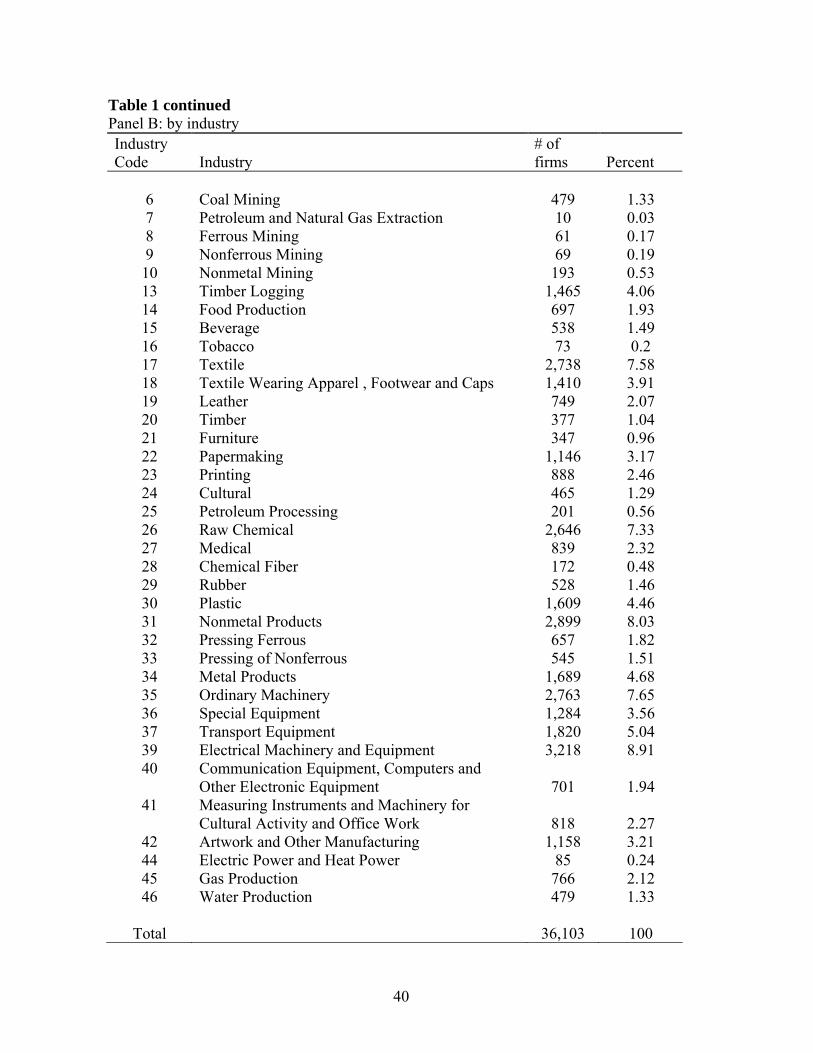
40

Table 1 continued Panel B: by industry Industry Code Industry

# of firms Percent

6 Coal Mining 479 1.33 7 Petroleum and Natural Gas Extraction 10 0.03 8 Ferrous Mining 61 0.17 9 Nonferrous Mining 69 0.19 10 Nonmetal Mining 193 0.53 13 Timber Logging 1,465 4.06 14 Food Production 697 1.93 15 Beverage 538 1.49 16 Tobacco 73 0.2 17 Textile 2,738 7.58 18 Textile Wearing Apparel , Footwear and Caps 1,410 3.91 19 Leather 749 2.07 20 Timber 377 1.04 21 Furniture 347 0.96 22 Papermaking 1,146 3.17 23 Printing 888 2.46 24 Cultural 465 1.29 25 Petroleum Processing 201 0.56 26 Raw Chemical 2,646 7.33 27 Medical 839 2.32 28 Chemical Fiber 172 0.48 29 Rubber 528 1.46 30 Plastic 1,609 4.46 31 Nonmetal Products 2,899 8.03 32 Pressing Ferrous 657 1.82 33 Pressing of Nonferrous 545 1.51 34 Metal Products 1,689 4.68 35 Ordinary Machinery 2,763 7.65 36 Special Equipment 1,284 3.56 37 Transport Equipment 1,820 5.04 39 Electrical Machinery and Equipment 3,218 8.91 40 Communication Equipment, Computers and

Other Electronic Equipment 701 1.94 41 Measuring Instruments and Machinery for

Cultural Activity and Office Work 818 2.27 42 Artwork and Other Manufacturing 1,158 3.21 44 Electric Power and Heat Power 85 0.24 45 Gas Production 766 2.12 46 Water Production 479 1.33

Total 36,103 100

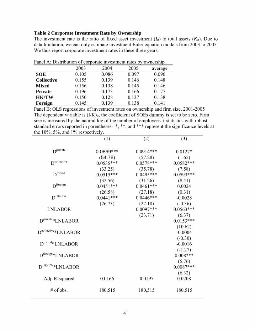
41

Table 2 Corporate Investment Rate by Ownership The investment rate is the ratio of fixed asset investment (Iit) to total assets (Kit). Due to data limitation, we can only estimate investment Euler equation models from 2003 to 2005. We thus report corporate investment rates in these three years. Panel A: Distribution of corporate investment rates by ownership 2003 2004 2005 average SOE 0.105 0.086 0.097 0.096 Collective 0.155 0.139 0.146 0.148 Mixed 0.156 0.138 0.145 0.146 Private 0.196 0.173 0.166 0.177 HK/TW 0.150 0.128 0.137 0.138 Foreign 0.145 0.139 0.138 0.141

Panel B: OLS regressions of investment rates on ownership and firm size, 2001-2005 The dependent variable is (I/K)it, the coefficient of SOEs dummy is set to be zero. Firm size is measured by the natural log of the number of employees. t-statistics with robust standard errors reported in parentheses. *, **, and *** represent the significance levels at the 10%, 5%, and 1% respectively. (1) (2) (3)

Dprivate

Dcollective

Dmixed

Dforeign

DHK/TW

LNLABOR

Dprivate*LNLABOR

Dcollective*LNLABOR

Dmixed*LNLABOR

Dforeign*LNLABOR

DHK/TW*LNLABOR

Adj. R-squared

# of obs.

0.0869***

(54.78) 0.0535***

(33.25) 0.0515***

(32.56) 0.0451***

(26.58) 0.0441***

(26.73)

0.0166

180,515

0.0914***

(57.28) 0.0578***

(35.78) 0.0495***

(31.26) 0.0461***

(27.18) 0.0446***

(27.18) 0.0097***

(23.71)

0.0197

180,515

0.0127* (1.65)

0.0582*** (7.58)

0.0593*** (8.41) 0.0024 (0.31)

-0.0028 (-0.36)

0.0563*** (6.37)

0.0153*** (10.62) -0.0004 (-0.30) -0.0016 (-1.27)

0.008*** (5.76)

0.0087*** (6.32) 0.0208

180,515

42

Table 3 Summary Statistics The table presents the summary statistics of the key variables used in our empirical analysis from 2001 to 2005 (year 2000 is not included because investment data for that year are not available). We drop from our sample the firms with extreme variable values (one percent at both tails). We obtain a panel with 36,103 firms in each year. The definition of variables can be found in the first column. Note that LNLABOR is the natural log of the number of the employees, NERI is a variable designed by Fan and Wang (2004) to examine the extent of marketization in each province in China, CFK is the ratio of cash flow to total assets, HIND is the Herfindahl index at the two-digit industry level, and finally, AGE captures firm age. Variable Obs Mean Std. Dev. Min Max Long term liabilities / total assets (TLTD)

180,515 0.064 0.121 0.000 0.726

Cash flow / total assets (CFK)

180,515 0.034 0.132 -0.469 0.950

Depreciation Rate (DRATE)

180,515 0.172 0.250 0.000 0.700

Total sales /total assets (ST)

180,515 1.274 1.037 0.060 9.525

Inventories / total assets (INVEN)

180,515 0.181 0.141 0.000 0.696

Income tax / total assets (TAX)

180,515 0.009 0.015 0.000 0.122

Sales costs / total assets (VC)

180,515 1.094 0.965 0.038 8.447

Current assets /total assets (CA)

180,515 0.031 0.024 0.000 0.182

Profits/total sales (INCOME)

180,515 0.027 0.083 -0.663 0.331

Investment Rate (Iit/Kit)

180,515 0.149 0.194 0.000 0.976

Industry Herfindahl index (HIND)

180,515 0.011 0.015 0.001 0.486

Firm size (LNLABOR)

180,515 5.354 1.138 0.000 11.903

LABOR

180,515 500.4 2082.1 30 147,722

NERI

180,515 6.294 1.583 3.910 9.740

Firm Age

180,515 16.120 13.854 1 105

43

Table 4 GMM Estimates of Investment Euler Equations on the Full Sample We estimate investment Euler equations on a sample of industrial firms from a database maintained by the National Bureau of Statistics of China (NBS). Our sample contains 36,103 industrial firms from 2001 to 2005. Nonlinear GMM estimations are conducted on the model in first differences with twice lagged instruments. There are in total 22 instruments in our estimations. α is the adjustment cost parameter to be estimated, and µ is a mark-up. Dprivate, Dcollective, Dmixed, Dforeign, DHK/TW and DSOE

are dummy variables indicating a firm’s ownership type. The estimated coefficients of DSOE, and DSOE*LNLABOR are set to be zero. LNLABOR is the natural logarithm of the number of the employees, CFK is the ratio of cash flow to total assets; HIND measures the industry-level Herfindahl index; TLTD is the ratio of long-term liabilities to total assets. NERI is a variable designed by Fan and Wang (2004) to examine the extent of marketization in each province in China. Standard errors are reported in parentheses. The p-values of the J-Test and L-Test on model specification are reported in the last two rows. *, **, and *** represent the significance levels at the 10%, 5%, and 1% respectively.

44

(1) (2) (3) (4) (5)

α

µ

Dprivate

Dcollective

Dmixed

Dforeign

DHK/TW

LNLABOR

Dprivate*LNLABOR

Dcollective*LNLABOR

Dmixed*LNLABOR

Dforeign*LNLABOR

DHK/TW*LNLABOR

HIND

NERI

TLTD

Chi-squared Degree of freedom

J-Test L-Test

0.072* (0.041) 1.011*** (0.055) -0.979*** (0.202) -1.038*** (0.235) -0.476 (0.361) -0.852*** (0.151) -0.896*** (0.279) -0.143*** (0.023) 0.167*** (0.038) 0.165*** (0.046) 0.068 (0.059) 0.152*** (0.024) 0.151*** (0.037) -1.275 (1.096) -0.021 (0.015) 0.048 (0.365) 6.531 6 0.366 n.a.

0.059** (0.031) 1.104*** (0.038) -1.098*** (0.329) -0.926*** (0.225) -1.315*** (0.326) -1.129*** (0.137) -1.067*** (0.232) -0.159*** (0.019) 0.179*** (0.057) 0.135*** (0.046) 0.207*** (0.050) 0.186*** (0.022) 0.167*** (0.029) -1.076 (0.661) 0.002 (0.016) 7.153 7 0.413 0.431

0.057** (0.026) 1.102*** (0.036) -1.175*** (0.177) -0.879*** (0.205) -1.163*** (0.219) -1.085*** (0.091) -0.991*** (0.143) -0.157*** (0.011) 0.202*** (0.034) 0.143*** (0.043) 0.193*** (0.032) 0.184*** (0.021) 0.163*** (0.019) -1.047* (0.591) 7.468 8 0.487 0.575

0.057** (0.027) 1.086*** (0.039) -1.068*** (0.173) -0.918*** (0.193) -1.281*** (0.193) -0.968*** (0.101) -0.852*** (0.125) -0.171*** (0.008) 0.174*** (0.034) 0.135*** (0.041) 0.202*** (0.029) 0.173*** (0.028) 0.149*** (0.021) 10.851 9 0.286 0.066

0.111* (0.061) 1.022*** (0.019) -0.307*** (0.059) -0.287*** (0.062) -0.335*** (0.072) -0.241** (0.102) -0.312*** (0.072) -0.098*** (0.012) 27.973 14 0.014 0.000

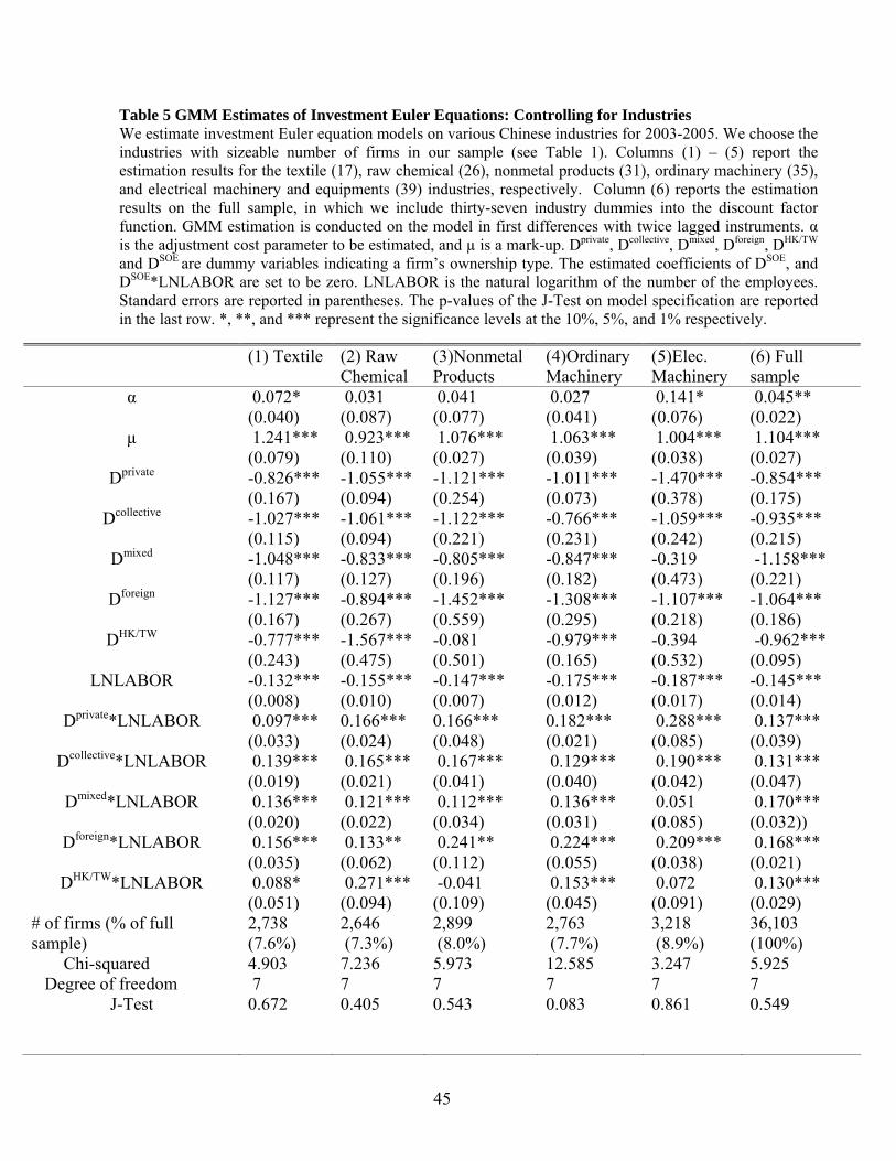
45

Table 5 GMM Estimates of Investment Euler Equations: Controlling for Industries We estimate investment Euler equation models on various Chinese industries for 2003-2005. We choose the industries with sizeable number of firms in our sample (see Table 1). Columns (1) – (5) report the estimation results for the textile (17), raw chemical (26), nonmetal products (31), ordinary machinery (35), and electrical machinery and equipments (39) industries, respectively. Column (6) reports the estimation results on the full sample, in which we include thirty-seven industry dummies into the discount factor function. GMM estimation is conducted on the model in first differences with twice lagged instruments. α is the adjustment cost parameter to be estimated, and µ is a mark-up. Dprivate, Dcollective, Dmixed, Dforeign, DHK/TW and DSOE

are dummy variables indicating a firm’s ownership type. The estimated coefficients of DSOE, and DSOE*LNLABOR are set to be zero. LNLABOR is the natural logarithm of the number of the employees. Standard errors are reported in parentheses. The p-values of the J-Test on model specification are reported in the last row. *, **, and *** represent the significance levels at the 10%, 5%, and 1% respectively.

(1) Textile (2) Raw Chemical

(3)Nonmetal Products

(4)Ordinary Machinery

(5)Elec. Machinery

(6) Full sample

α

µ

Dprivate

Dcollective

Dmixed

Dforeign

DHK/TW

LNLABOR

Dprivate*LNLABOR

Dcollective*LNLABOR

Dmixed*LNLABOR

Dforeign*LNLABOR

DHK/TW*LNLABOR

# of firms (% of full sample) Chi-squared Degree of freedom

J-Test

0.072* (0.040) 1.241*** (0.079) -0.826*** (0.167) -1.027*** (0.115) -1.048*** (0.117) -1.127*** (0.167) -0.777*** (0.243) -0.132*** (0.008) 0.097*** (0.033) 0.139*** (0.019) 0.136*** (0.020) 0.156*** (0.035) 0.088* (0.051) 2,738 (7.6%) 4.903 7 0.672

0.031 (0.087) 0.923*** (0.110) -1.055*** (0.094) -1.061*** (0.094) -0.833*** (0.127) -0.894*** (0.267) -1.567*** (0.475) -0.155*** (0.010) 0.166*** (0.024) 0.165*** (0.021) 0.121*** (0.022) 0.133** (0.062) 0.271*** (0.094) 2,646 (7.3%) 7.236 7 0.405

0.041 (0.077) 1.076*** (0.027) -1.121*** (0.254) -1.122*** (0.221) -0.805*** (0.196) -1.452*** (0.559) -0.081 (0.501) -0.147*** (0.007) 0.166*** (0.048) 0.167*** (0.041) 0.112*** (0.034) 0.241** (0.112) -0.041 (0.109) 2,899 (8.0%) 5.973 7 0.543

0.027 (0.041) 1.063*** (0.039) -1.011*** (0.073) -0.766*** (0.231) -0.847*** (0.182) -1.308*** (0.295) -0.979*** (0.165) -0.175*** (0.012) 0.182*** (0.021) 0.129*** (0.040) 0.136*** (0.031) 0.224*** (0.055) 0.153*** (0.045) 2,763 (7.7%) 12.585 7 0.083

0.141* (0.076) 1.004*** (0.038) -1.470*** (0.378) -1.059*** (0.242) -0.319 (0.473) -1.107*** (0.218) -0.394 (0.532) -0.187*** (0.017) 0.288*** (0.085) 0.190*** (0.042) 0.051 (0.085) 0.209*** (0.038) 0.072 (0.091) 3,218 (8.9%) 3.247 7 0.861

0.045** (0.022) 1.104*** (0.027) -0.854*** (0.175) -0.935*** (0.215) -1.158*** (0.221) -1.064*** (0.186) -0.962*** (0.095) -0.145*** (0.014) 0.137*** (0.039) 0.131*** (0.047) 0.170*** (0.032)) 0.168*** (0.021) 0.130*** (0.029) 36,103 (100%) 5.925 7 0.549

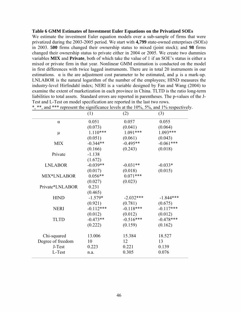
46

Table 6 GMM Estimates of Investment Euler Equations on the Privatized SOEs We estimate the investment Euler equation models over a sub-sample of firms that were privatized during the 2003-2005 period. We start with 4,799 state-owned enterprises (SOEs) in 2003. 500 firms changed their ownership status to mixed (joint stock); and 98 firms changed their ownership status to private either in 2004 or 2005. We create two dummies variables MIX and Private, both of which take the value of 1 if an SOE’s status is either a mixed or private firm in that year. Nonlinear GMM estimation is conducted on the model in first differences with twice lagged instruments. There are in total 20 instruments in our estimations. α is the are adjustment cost parameter to be estimated, and µ is a mark-up. LNLABOR is the natural logarithm of the number of the employees; HIND measures the industry-level Hirfindahl index; NERI is a variable designed by Fan and Wang (2004) to examine the extent of marketization in each province in China. TLTD is the ratio long-term liabilities to total assets. Standard errors are reported in parentheses. The p-values of the J-Test and L-Test on model specification are reported in the last two rows. *, **, and *** represent the significance levels at the 10%, 5%, and 1% respectively. (1) (2) (3)

α

µ

MIX

Private

LNLABOR

MIX*LNLABOR

Private*LNLABOR

HIND

NERI

TLTD

Chi-squared Degree of freedom

J-Test L-Test

0.051 (0.073) 1.110*** (0.051) -0.344** (0.166) -1.138 (1.672) -0.039** (0.017) 0.056** (0.027) 0.231 (0.465) -1.579* (0.921) -0.112*** (0.012) -0.473** (0.222) 13.006 10 0.223 n.a.

0.057 (0.041) 1.091*** (0.061) -0.495** (0.243) -0.031** (0.018) 0.071*** (0.023) -2.032*** (0.781) -0.118*** (0.012) -0.516*** (0.159) 15.384 12 0.221 0.305

0.055 (0.064) 1.093*** (0.043) -0.061*** (0.018) -0.033* (0.015) -1.844*** (0.675) -0.117*** (0.012) -0.478*** (0.162) 18.527 13 0.139 0.076

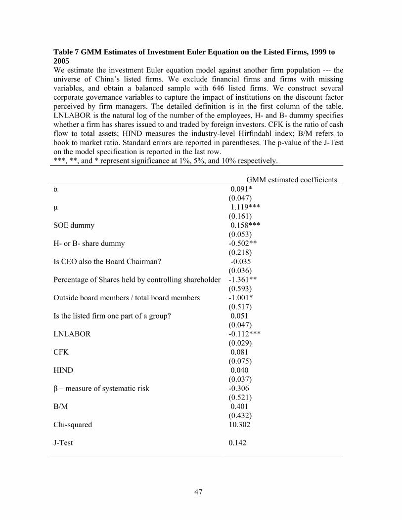
47

Table 7 GMM Estimates of Investment Euler Equation on the Listed Firms, 1999 to 2005 We estimate the investment Euler equation model against another firm population --- the universe of China’s listed firms. We exclude financial firms and firms with missing variables, and obtain a balanced sample with 646 listed firms. We construct several corporate governance variables to capture the impact of institutions on the discount factor perceived by firm managers. The detailed definition is in the first column of the table. LNLABOR is the natural log of the number of the employees, H- and B- dummy specifies whether a firm has shares issued to and traded by foreign investors. CFK is the ratio of cash flow to total assets; HIND measures the industry-level Hirfindahl index; B/M refers to book to market ratio. Standard errors are reported in parentheses. The p-value of the J-Test on the model specification is reported in the last row. ***, **, and * represent significance at 1%, 5%, and 10% respectively.

GMM estimated coefficients

α µ SOE dummy H- or B- share dummy Is CEO also the Board Chairman?

Percentage of Shares held by controlling shareholder Outside board members / total board members Is the listed firm one part of a group? LNLABOR CFK HIND β – measure of systematic risk B/M Chi-squared J-Test

0.091* (0.047) 1.119*** (0.161) 0.158*** (0.053) -0.502** (0.218) -0.035 (0.036) -1.361** (0.593) -1.001* (0.517) 0.051 (0.047) -0.112*** (0.029) 0.081 (0.075) 0.040 (0.037) -0.306 (0.521) 0.401 (0.432) 10.302 0.142

48

Table A1 GDP, Fixed Asset Investment, and FDI in China 1990-2005 Source: China Statistical Yearbook Exchange rate: 1 US$ = RMB 8.026

Year Gross Domestic Product

(RMB bn)

Fixed asset investment (RMB bn)

Percent of GDP

Foreign Direct

Investments (USD bn)

Percent of GDP

1990 1871.8 451.7 24.13% 3.49 1.50% 1991 2182.6 559.5 25.63% 4.37 1.61% 1992 2693.7 808.0 30.00% 11.01 3.28% 1993 3526.0 1307.2 37.07% 27.52 6.26% 1994 4810.9 1704.3 35.43% 33.77 5.63% 1995 5981.1 2001.9 33.47% 37.52 5.03% 1996 7014.3 2291.4 32.67% 41.73 4.77% 1997 7765.3 2494.1 32.12% 45.26 4.68% 1998 8302.4 2840.6 34.21% 45.46 4.39% 1999 8818.9 2985.5 33.85% 40.32 3.67% 2000 9800.1 3291.8 33.59% 40.72 3.33% 2001 10806.8 3721.4 34.44% 46.88 3.48% 2002 11909.6 4349.9 36.52% 52.74 3.55% 2003 13517.4 5556.7 41.11% 53.51 3.18% 2004 15958.7 7047.7 44.16% 60.63 3.05%

2005 18395.6 8877.4 48.26% 60.33 2.63%

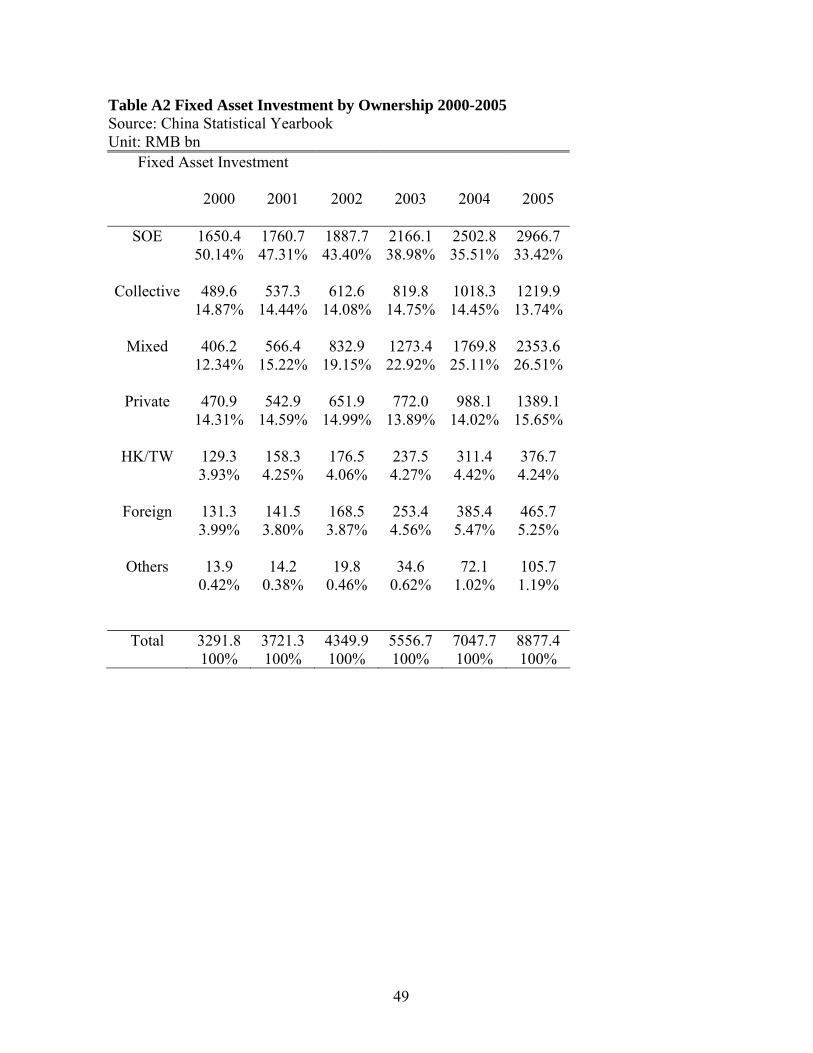
49

Table A2 Fixed Asset Investment by Ownership 2000-2005 Source: China Statistical Yearbook Unit: RMB bn

Fixed Asset Investment 2000 2001 2002 2003 2004

2005

SOE 1650.4 1760.7 1887.7 2166.1 2502.8 2966.7 50.14% 47.31% 43.40% 38.98% 35.51% 33.42%

Collective 489.6 537.3 612.6 819.8 1018.3 1219.9 14.87% 14.44% 14.08% 14.75% 14.45% 13.74%

Mixed 406.2 566.4 832.9 1273.4 1769.8 2353.6 12.34% 15.22% 19.15% 22.92% 25.11% 26.51%

Private 470.9 542.9 651.9 772.0 988.1 1389.1 14.31% 14.59% 14.99% 13.89% 14.02% 15.65%

HK/TW 129.3 158.3 176.5 237.5 311.4 376.7 3.93% 4.25% 4.06% 4.27% 4.42% 4.24%

Foreign 131.3 141.5 168.5 253.4 385.4 465.7 3.99% 3.80% 3.87% 4.56% 5.47% 5.25%

Others 13.9 14.2 19.8 34.6 72.1 105.7 0.42% 0.38% 0.46% 0.62% 1.02% 1.19%

Total 3291.8 3721.3 4349.9 5556.7 7047.7 8877.4 100% 100% 100% 100% 100% 100%

50

Table A3 The Breakdown of Sample Firms by Region Code Region # of firms Percent

11 Beijing 993 2.75 12 Tianjin 936 2.59 13 Hebei 1,337 3.7 14 Shanxi 511 1.42 15 Inner Mongolia 292 0.81 21 Liaoning 1,352 3.74 22 Jilin 337 0.93 23 Heilongjiang 357 0.99 31 Shanghai 2,664 7.38 32 Jiangsu 4,911 13.6 33 Zhejiang 5,399 14.95 34 Anhui 649 1.8 35 Fujian 2,254 6.24 36 Jiangxi 284 0.79 37 Shandong 2,561 7.09 41 Henan 1,313 3.64 42 Hubei 590 1.63 43 Hunan 364 1.01 44 Guangdong 4,721 13.08 45 Guangxi 488 1.35 46 Hainan 100 0.28 50 Chongqing+Sichuan 1,666 4.61 52 Guizhou 403 1.12 53 Yunnan 537 1.49 54 Tibet+Qinghai+Ningxia 121 0.34 61 Shaanxi 502 1.39 62 Gansu 235 0.65 65 Xinjiang 226 0.63

Total 36,103 100

51

Figure 1 The Investment-Implied Return on Captial By Ownership: 2001-2005

0

0.02

0.04

0.06

0.08

0.1

0.12

0.14

0.16

2001 2002 2003 2004 2005

SOE Collective Mixed Private HK/TW Foreign

Note: We plug the variable values for each firm into the estimated discount factor function as specified in Model 3 of Table 4 (the benchmark model). We make an assumption that the average discount rate for all of the firms in our sample is 10%. We thus back out the value of the intercept in the discount factor function, 1.904. We then compute the investment-implied discount rate for each firm in each year. We aggregate those firm-year observations by ownership and year.