CAHIER DE RECHERCHE #1606E WORKING PAPER #1606E Département de science économique Department of Economics Faculté des sciences sociales Faculty of Social Sciences Université d’Ottawa University of Ottawa

Ronan Congar* and Louis Hotte†

May 2016

This is a much revised and expanded version of an earlier one, with many new results, that circulated under the title “Open Access vs. Restricted Access with Two Variable Factors: On the Redistributive Effects of a Property Regime Change”. It has benefited from comments by Stefan Ambec, Victoria Barham, Brian Copeland, Pierre Lasserre and seminar participants at the University of Ottawa, Université de Rouen, the 2012 CREE Meetings at UBC, the 2012 Conference on Environment and Natural Resources Management in Developing and Transition Economies at Université d’Auvergne, the 2014 Montreal Natural Resources and Environmental Economics Workshop at McGill University, Economix at Université Paris Ouest Nanterre La Défense, the University of Queensland and the Congreso Sobre México 2015 at Universidad Iberoamericana. We are responsible for any remaining error. * EconomiX, UMR CNRS 7235 Université Paris Ouest - Nanterre La Défense and Department of Economics, University of Ottawa, 120 University Private, Ottawa, Ontario, Canada, K1N 6N5; e-mail: ronan.congar@gmail.com. † Department of Economics, University of Ottawa, 120 University Private, Ottawa, Ontario, Canada, K1N 6N5; e-mail: louis.hotte@uottawa.ca.

Institutional Reform in the Rural Sector with Labor and Capital Flows: Factor Income Effects, Structural Changes and Misallocations

Abstract We analyze the general equilibrium effects of a fundamental property regime transition in the rural sector - agricultural or resource - when both labor and (reproducible) capital are free to move. In contrast to manufacturing, rural production has two characteristic features: it uses a fixed natural asset (land or other natural resources) and operates under one of two property regime types: common property versus exclusive property. Common property is fundamentally characterized with sharing, thus corresponding to such institutions as the family farm (Lewis 1954), free access to resources, and collective use, but adapted for the presence of capital use. We show that labor may actually gain from being effectively forced out of the rural sector. More generally, relative factor intensities determine the factor return effects of the transition, as well as either capital or labor deepening in both sectors. And while the unit cost of effective input efforts decrease, both factors flow out of the rural sector. Under a common property regime, the agricultural productivity gaps for labor and capital are uniquely determined by the output elasticity of land. Key words: Institutions, Property Rights, Agriculture, Natural Resources, Factor Migration, Factor Returns, Redistribution, Factor Misallocation, Structural Changes, Agrarian Reform, Resource Privatisation JEL Classification: D02, D23, D33, L16, N50, O13, O15, O17, Q15.

1 Introduction

Among the various processes associated with economic development, the transition froman agrarian or resource-based economy to a manufacturing one arguably constitutes itsmost remarkable expression. It transforms people’s lives - for better or worse - and it isunescapable. Now among the few fundamental factors that together explain this transition,institutional change in the agricultural and resource sectors figures prominently. In thispaper, we propose a new analysis of structural change brought about by the adoption of“modern” market institutions in the agrarian or resource sector. It differs from existingones in that we allow for the free flow of both labor and capital, while accounting for thepresence of fixed natural assets such as land and other natural resources. One significantimplication is to show that labor may actually gain from being denied the rents from thenatural assets. The economic forces at work provide new insights into the links betweeninstitutions and factor misallocation, factor migration, income distribution, factor intensity,capital deepening and productivity gaps. We can’t underscore enough the fact that ourresults hinge on the presence of mobile capital and a fixed natural asset; while both arerecognized as crucial to our understanding of structural changes, their combined presenceseems to have escaped careful general equilibrium consideration in relation to institutionalchange.

The “traditional” property regime that we consider is referred to as common property.Its essential feature is that rents on the natural asset are shared between the users. Thissharing property is mainly inspired by two fundamental institutions commonly analysed intwo separate strands of the economics literature and it is still widely used in both empiricaland theoretical work. One is the institution of the family farm as described in Lewis (1954)and Ranis and Fei (1961); it pervades the development economics literature, especially inrelation to labor misallocations and rural-urban migration. The other is the regime of freeaccess to natural resources as described in Gordon (1954) and Cheung (1970); it constitutesa founding block of the natural-resource economics literature. In the case of Lewis’ familyfarm, we adapt it for the use of capital as an input; this, to our knowledge, constitutes anovelty.1 This leads us to propose an equivalence result between the sharing family farmand the free-access equilibrium concepts with capital inputs.

Based on a collection of empirical cases provided in the text as illustrative of other “pre-capitalist” institutions, we conclude that the common property regime captures well one ofthe root causes of factor misallocations between the rural and manufacturing sectors. But

1The consideration of the use of capital by farmers in developing economies is consistent with Gollin’s(2014) statement that “[Lewis’] assumption that only capitalists can invest productively seems inconsistentwith current micro and macro evidence on savings behavior and investment. (83)” Note further that ouranalysis does not make use of the subsistence wage or surplus labor concepts, as they have not receivedmuch empirical support; the sharing property, on the other hand, is considered valid to this day. See thediscussions in Ray (1998:360) and Gollin (2014).

2

while the sharing condition is still extensively used to explain the misallocation of labor byrelying on the distinction between labor’s average and marginal product values, it has largelyignored the concurrent effects on endogenous capital misallocations. Our analysis fills thisgap.

The other property regime that we consider simply corresponds to the exclusive use ofland or natural resources by one entity that seeks to maximize rents with the right choiceof inputs. This is referred to as exclusive property and leads to the first-best allocation offactors.

From a theoretical perspective, our general equilibrium approach is mainly inspired byWeitzman (1974) and Cohen and Weitzman (1975). We consider an economy with twosectors only, referred to as rural and manufacturing here, where production in the ruralsector requires the use of a fixed natural asset. We then compare two general equilibriadepending on the property regime that prevails on the natural asset: common propertyversus exclusive property. While Weitzman (1974) considers labor to be the only mobilefactor between the sectors, we add (reproducible) capital as a second mobile factor. Thissimple distinction yields many new results and insights. Foremost among them concernsthe famous proposition that resource privatization causes labor wages to decrease. Indeed,we show that this result is not robust to the addition of capital as a mobile factor. Thenecessary and sufficient condition for wages to increase and capital returns to decrease is thatthe manufacturing sector be relatively labor intensive (in a way that we define precisely).We then provide empirical evidence to the effect that this condition is likely to be verifiedin many settings and conjecture that an important distinction may have to be made herebetween wheat and rice growing agricultural economies.

The fact that labor may gain from being effectively forced out of the rural sector seemsparadoxical. But keep in mind that capital follows labor. Hence, as both factors move intothe manufacturing sector in (generally) unequal proportions, factor intensities are affectedand thus, factor returns change in opposite directions. The distinction is analogous to thatmade between the specific-factors and the Heckscher-Ohlin models of trade.2 By analogy,our model may be conceived as providing the long-run effects of institutional change. Thatsaid, we retain the realistic and crucial feature that land or natural resources constituteimportant fixed inputs to the rural sector. Note finally that just like the Hecksher-Ohlinframework, our analysis is static in the sense that total factor endowments are consideredfixed throughout.3

2Recall that the specific-factors model assumes that only labor can move between sectors while capitalis riveted to its respective sector and as such, is viewed as delivering the short-run effects of trade. TheHeckscher-Ohlin framework posits a free flow of labor and capital between sectors and this is interpreted asdelivering a long-term view of the effects of trade. See Jones (1971), Mayer (1974) and Mussa (1974), orstandard trade theory textbooks.

3It goes without saying that a dynamic version would yield additional insight. This is left for furtherwork. As Temple (2005) rightfully contends, “It is a mistake to think that an understanding of economic

3

Our analysis yields additional contributions. We derive the conditions that characterizea common property equilibrium in the presence of three factors of production, one fixed andtwo mobile. In doing so, we propose a novel microeconomic dual approach that yields newinsights into the structural changes brought about by a fundamental property regime change.We then show that the transition causes the price of one mobile factor to decrease and theother to increase, the net effect being an overall decrease in the unit cost of effective inputefforts in the rural sector. Both labor and capital will nonetheless leave the rural sector. Wefurther show that, under the same conditions that cause wages to increase, the transitioncauses a general capital deepening of the production processes even though the aggregatecapital-labor ratio is unchanged. Finally, with the use of Cobb-Douglas technologies, weshow that the agricultural productivity gaps of labor and capital are uniquely dictated bythe output elasticity of the natural asset.

In the natural-resource literature, Weitzman’s (1974) proposition that wages would benegatively affected by resource privatization while being more efficient has sparked a liter-ature which extended the model’s basic assumptions into various directions. This includesAnderson and Hill (1983) on transaction costs, Brooks and Heijdra (1990) on enforcementlabor, Intriligator and Sheshinski (1997) on a heterogeneous labor force and Ambec andHotte (2006) on imperfect enforcement. None of these, however, discusses the role of capital.To our knowledge, de Meza and Gould (1987) is the only paper that hints at the potentiallyimportant role of a second variable factor, but the analysis is not carried out. Our modelis also inspired by Karp (2005), who argues that when considering the interactions betweentrade openness, property regimes, and natural resource use, one should treat both labor andcapital as mobile factors between the resource and manufacturing sectors. This is in responseto previous analysis that ignored the role of capital, such as Chichilnisky (1994), Branderand Taylor (1997) and Hotte, Long and Tian (2000). Karp (2005), however, focuses on thelink between trade openness and the excludability of capital use.

In the lineage of the Lewis (1954) model and “dualism” in development economics, theliterature is quite extensive and the reader is referred to the two excellent reviews by Temple(2005), who “argues that dual economy models deserve a central place in the analysis ofgrowth in developing countries (435)”, and Gollin (2014), who believes that “the modelremains a powerful and useful tool for thinking about growth because it correctly identifies akey feature of the growth process – namely, the importance of within-country gaps in incomeand productivity, or dualism. (73)” One noteworthy paper is Drazen and Eckstein (1988)who similarly compare different property regimes but under the assumption that agriculturalproduction does not require capital. Regarding dualism, the closest paper to ours in spiritmay be that of Corden and Findlay (1975), who look at the effects of introducing capitalmobility into the Harris and Todaro (1970) framework. The Lewis model being consideredthe main “competing” model to the Harris-Todaro one regarding rural-urban migrations

development can only ever be gained by analysing dynamic models... (439)”

4

(Ray 1998), performing the exercise in the Lewis context seems overdue.Our analysis is equally motivated by the burgeoning literature on the economics of growth

that looks at factor misallocations between the agricultural sector and other sectors. Itgenerally concludes that a large share of cross-country variations in aggregate total-factorproductivity can be explained this way. This work includes Caselli (2005), Temple andWossmann (2006), Restuccia et al. (2008), Vollrath (2009), Adamopoulos and Restuccia(2014) and Gollin et al. (2014a). This literature has begun to spark renewed interest into theeconomic determinants of factor misallocations. Young (2013) and Munshi and Rosenzweig(2016), for instance, respectively look at the roles of human capital and networks. Ouranalysis complements this work and goes some way into addressing the specific grievancesexpressed in Foster and Rosenzweig (2008) about the call for future work “... to developa more comprehensive simple general-equilibrium model of a rural economy incorporatingfactor flows [...] both capital and labor (3052-54)”, to account for “the presence of a dominantfixed factor in agricultural production (land) (3053)”, and that “... careful considerationneeds to be given to the extent to which migrant households lose their claim on local assetswhen they migrate (3081)”.

The paper is organised as follows. In Section 2, the economy is defined with productiontechnologies, endowments, and institutions. Sectoral equilibrium conditions are laid outin Section 3 for each property arrangement. Section 4 presents the factor-payment anddisplacement effects of a property regime transition. Some empirical implications regardingrelative factor intensities and productivity analysis are discussed in Section 5. The conclusionoffers avenues for future research.

2 The economy: Endowments, technologies and institutions

Production requires three types of factors: labor, reproducible capital, and natural (non-reproducible) capital, with respective fixed total endowments L, K and T . We think of Tas a country’s natural resource endowment such as the total extent of its agricultural landsurfaces, the size of its fishing grounds, the availability of underground minerals and water,or its forests.4 To avoid confusion, reproducible capital will be referred to as K-capital.

The economy is composed of two main sectors. While we will refer to them as rural(R) and manufacturing (M) for concreteness, they are really distinguished by two essentialfeatures. One concerns the factor requirements for production: the manufacturing sectorneeds only labor and reproducible capital; the rural sector needs all three factors. The otherconcerns the fact that two types of property regimes may prevail over the natural asset.Hence, depending on the reference literature, our rural and manufacturing dichotomy typ-

4Note that we abstract from stock-flow dynamics regarding soil quality or other renewable and non-renewable resources. We leave that for required future work as we wish to concentrate on the interactionsbetween the change of institutional setting and capital mobility.

5

ically corresponds to agricultural and non-agricultural when discussing structural changes,rural and urban for migration analysis, natural resource and manufacturing for propertyregime changes, traditional and modern for dual economies, or the distinction made betweenagriculture and rural non-farm activities by Foster and Rosenzweig (2008). It should becomeclear that our analysis is of relevance to all these literatures.

Since both sectors require labor and reproducible capital, we refer to these as the mobile(or variable) factors. The natural capital is called the fixed factor because its size cannot bevaried in the rural sector.

2.1 The manufacturing sector

Manufactures are produced using labor LM and K-capital KM only, with a constant returnsto scale technology. The output Y M of the entire manufacturing sector is thus representedby the following relation:

Y M = FM(LM , KM), (1)

where function FM is twice continuously differentiable, strictly quasi-concave, homogeneousof degree one, increasing in both arguments and such that FM(0, 0) = 0.

2.2 The rural sector

In order to produce rural goods, all three factor types are required: labor LR, K-capital KR,and the fixed factor T .

It is important to keep in mind that even among poor rural communities, reproduciblecapital may play an important role in farming. Indeed, because the K-capital input inagriculture is often construed as being only composed of machines and structures such astractors, plows, barns or silos, one is often led to believe that due to their scarcities indeveloping economies (or in medieval times), agriculture is (was) a predominantly labor-usingactivity. This is misleading because reproducible capital in agriculture also includes livestock(sheeps, cows, bullocks, etc) and treestock (orchards, plantations, etc).5 This agriculturalcapital incorporates all of the fundamental features of machinery: it is a productive assetthat can be imperfectly substituted for land and labor; it is produced; it is rival in use; andit depreciates. Of particular relevance to us is the fact that it is the fruit of an investmentwith “time-to-build” and depreciation.6 This means that in the medium to long run, asavings stock can be moved from one sector’s K-capital investment to another as relative

5See, for instance, Jarvis (1974), Jorgenson and Gollop (1992), Rosenzweig and Wolpin (1993), Mundlak(2001) and Mundlak et al. (2012).

6See, for instance, Rosen et al. (1994) and Fafchamps (1998).

6

factor payoffs vary.7

We assume constant returns to scale in the three-input vector (LR, KR, T ). But becauseT is fixed, production in the rural sector really exhibits decreasing returns to scale withrespect to the variable input vector (LR, KR). For simplicity, the rural output can simplybe represented as a function of the two variable inputs. We accordingly represent the ruralproduction technology as follows.

Let the individual effective effort exerted on the fixed asset by individual i be expressed asZi = FR(LR

i , KRi ), where L

Ri and KR

i respectively denote the amounts of labor and K-capitalinputs supplied by rural worker i. Function FR is assumed twice continuously differentiable,strictly quasi-concave, homogeneous of degree one, increasing in both arguments and suchthat FR(0, 0) = 0.

With n individuals active in the rural sector, let the total output produced in the ruralsector be given by Y R = f(Z), where Z =

∑n

i=1Zi is the total effective effort. Function f

is twice continuously differentiable, increasing, strictly concave and such that f(0) = 0.8 Tosummarize, we have:9

Y R = f(Z), f ′ > 0, f ′′ < 0, [total rural output] (2)

Z =n∑

i=1

Zi where Zi = FR(LRi , K

Ri ). [rural effective input effort] (3)

2.3 The institutional settings

Producers are price takers throughout, for both inputs and outputs. We assume a smallopen economy for which output prices are exogenously fixed on world markets. Factor priceswill however be endogenously determined by the general equilibrium conditions. Labor andK-capital are free to move between sectors.

In the case of labor and K-capital, we assume that there are no property right issues inthe sense that they are both perfectly excludable at no cost. Owners of these factors willthus seek to maximize their respective payoff.

The focus of our analysis will be to compare equilibria when either of two differentproperty regimes prevail over the fixed factor used in the rural sector. For clarity, we referto the payoff from the fixed asset as a rent. We define the two regimes as follows:

7The shift in agricultural production observed in England after the Black Death (1348-1350) provides aninteresting historical example. The reasoning is that as the plague wiped out close to half of the population,the relative cost of labor increased in such a way that farmers shifted a good share of their land use fromarable to (sheep) pasture, the later being much more capital-intensive, and the transition spread-out overmany years in part because of the time needed to build up the livestock (Campbell et al. 1996).

8The strict concavity assumption for f , combined with constant returns to scale for FR, insures that wehave decreasing returns to scale on (LR,KR), where LR =

∑n

i=1LRiand KR =

∑n

i=1KR

i.

9Note that the rural sector is composed of just one site for simplicity. The presence of multiple siteswould not alter the qualitative nature of our results given that we assume price-taking behavior throughout.

7

Definition 1 Under exclusive property (EP), the totality of the rents generated by the nat-ural asset accrue to its owner(s) independently of its (their) labor and K-capital inputs. Theowner(s) can perfectly and costlessly control the amounts of both labor and K-capital to beused on this asset.

Definition 2 Under common property (CP), rents are distributed between all individualswho actively work on the natural asset with their labor input. Rent shares are proportionalto the effective input effort. Moreover, no worker can be expelled from using the naturalasset.

Exclusive property corresponds to the standard situation of total rent maximization forthe fixed asset. Common property, in contrast, does not lead to rent maximization. Aswe demonstrate below, it rather leads to an equalization between the average return perworker on the fixed asset and the wage rate that prevails in the rest of the economy.10 Thisequalization result is not new to the literature, to be sure. This literature, however, typicallyconsiders labor to be the sole variable factor. With K-capital as a second variable factor,the corresponding equilibrium condition will need to be carefully adapted.

We believe that the equilibrium conditions that we derive for the intersectoral allocationof K-capital and labor in the common property regime constitute a fair representation oftraditional or pre-capitalist institutions such as the family farm in developing countries ingeneral, common property land or resources in medieval Europe, collective farming, andopen-acces to natural resources such as fishing grounds.

Note that we do not mean to imply that the above-mentioned institutions are equivalentin all respects.11 However, they do share one very fundamental feature, which is that rentstend to be shared between those who work on the land or resource and that the choice ofstaying or not belongs to the individual rather than the group. The following presents a listof well-known, representative cases.

The sharing argument for the family farm dates back to Lewis 1954 and has a long tradi-tion in the economics of migration (Ray 1998). More recently, Foster and Rosenzweig (2008)provide empirical evidence that suggests “that migrants in fact do give up at least someof agricultural profits when they leave” (3076). In the case of medieval England, Cohenand Weitzman (1975) argue that under open field agriculture, there was an “equalizing ten-dency” within and between villages and that “We have no evidence that villagers attemptedto exclude a newcomer” (298). Zhao (2015) explains that before a rural land reform in 2003in China, “land [was] collectively owned at the village level” (1) and shows that land wasfrequently reallocated in order to equalize per-capita output between the village households.

10 In the normative literature on rules of division, our common property regime corresponds to the pro-

portional allocation rule in Roemer (2015).11Carter (1984), for instance, states that due to a lower information burden, incentives to free-ride on the

effort of others are less acute on the family farm than for collective farming.

8

Regarding a land reform in Russia in 1906, Chernina et al. (2014) mention that “[...] theopportunity cost of migration decreases [following a switch from communal to individualownership] because owners are able to better extract land rent without being physicallypresent” (192). For the decollectivization of agriculture in Eastern Europe that began in1989, Mathijs and Swinnen (1998) state that “A crucial factor that determines decollec-tivization is the ratio of the average labor productivity of an individual farm started up byan individual who left the collective farm over the average labor productivity of the collectivefarm” (7). For the case of open-access to natural resources, the link with the average productof input efforts is well known and is attributed to Gordon (1954). The discussion over tiedrents in Lucas (1997) is also consistent with our definition of common property.

Note finally that our common property regime is consistent with the Ranis and Fei (1961)assumption of an agricultural wage that is determined by an “institutional force” instead of a“subsistence wage”, which Gollin (2014) presents as the more empirically relevant applicationof the Lewis model. And though we agree with Gollin (2014) that rents are rarely sharedperfectly equally, the fact that some sharing is going on between on-site users implies that theassumption of rent maximization and equality of labor’s marginal products is not realisticeither. Given this, the equilibrium conditions that we will derive under perfect sharingamong workers seem like a fair approximation to make in order to contribute to a literaturethat has generally ignored the role of K-capital mobility with a fixed asset.

3 Equilibrium conditions

We take manufactures as the numeraire good. w and r denote the respective prices of laborand K-capital. p is the price of the rural good, exogenously fixed on world markets. Weconsider only interior solutions in which both sectors are simultaneously active. For themobile factors, the following market clearing conditions apply throughout:

LM + LR = L and KM +KR = K. (4)

3.1 Manufacturing sector

In order to maximize profits, manufacturers simply equate marginal product values withfactor prices, i.e.,12

FML (LM , KM) = w and FM

K (LM , KM) = r. (5)

In order to represent the equilibrium in the manufacturing sector, it will also be conve-nient to make use of the cost-minimization dual to (5). Given constant-returns to scale, the

12The subscript of a function denotes a partial derivative.

9

unit cost of producing one unit of manufacturing output depends on factor prices only andis denoted cM(w, r); this function has the usual properties of a cost function. Since manu-factured goods are used as numeraire goods, the equilibrium in the manufacturing sector isrepresented by the following zero-profit condition:

cM(w, r) = 1. (6)

3.2 Rural sector

Equilibrium conditions in the rural sector depend on which property regime prevails.

3.2.1 Exclusive property (EP)

Under EP, the rural owner(s) – say a firm with share-holders – gets to choose variable inputvector (LR, KR) by hiring labor and K-capital in order to maximize profits. The problem ofthe firm is

maxLR,KR

π = pf(Z)− [wLR + rKR], (7)

where Z = FR(LR, KR). This yields the following pair of first-order conditions:

pf ′(Z)FRL (LR, KR) = w (8)

pf ′(Z)FRK (LR, KR) = r. (9)

These conditions simply state that under EP, the owner equates the marginal product valueof each variable factor to its cost. The circumflex symbol will refer to the EP equilibrium.

From the perspective of cost minimization, as a profit maximizer, the owner seeks to min-imize the cost of any realized exploitation effort level Z. Now given that Z = FR(LR, KR),that FR exhibits constant returns to scale, and price taking, the unit cost of Z is consideredconstant by the firm and dependent on input vector cost (w, r). As a result, letting cR(w, r)denote the unit cost of Z, the problem of the owner can also be expressed as follows:

maxZ

π = pf(Z)− ZcR(w, r). (10)

The owner’s optimal exploitation effort is thus given by

pf ′(Z) = cR(w, r). (11)

Conditions (8) and (9) are equivalent to (11) as a way to represent the EP exploitation levelin the rural sector.

10

3.2.2 Common property (CP)

In the CP regime, worker i must choose her individual effective effort level Zi = FR(LRi , K

Ri )

to spend on the common asset. We assume that a worker inelastically supplies a total of oneunit of labor and that one cannot split her time between the rural and the manufacturingsectors; hence, LR

i = 1 and thus LR = n. In the case of K-capital, each worker can hire anyamount at rental cost r. Given that output is shared in proportion to the effective effort, i’snet payoff is thus given by:

πi = pf(Z)Zi

Z− rKR

i , (12)

where Zi = FR(1, KRi ) and Z =

∑n

i=1Zi. One notes that under common property, each

worker is remunerated according to the average product of effective effort on the fixed asset.For analytical convenience, let us define the following average product function: φ(Z) ≡f(Z)/Z. In order to simplify the analysis, we assume that each rural worker takes theaverage product as given when deciding on her individual effort.13 The first-order conditionfor i’s choice of capital input is thus:

∂πi

∂KRi

= pφ(Z)FK(1, KR∗

i )− r = 0. (13)

This condition can be interpreted as follows. Adding one marginal unit of K-capital willincrease the effective effort by FR

K . This increase is then multiplied by the average productof effective effort in order to arrive at the extra output received by user i; this increaseexceeds the overall increase because it ignores the cost imposed on other users in terms ofreduced average product of effective effort. The only cost that each user accounts for is thedirect cost of K-capital r. This contrasts with EP condition (9), where multiplication withthe marginal product of effective effort insures that the drop in average product of all usersis well accounted for by the exclusive owner.

With identical workers and the fact that function FR has constant returns to scale, (13)implies that

FRK (LR, KR∗) =

r

pφ(Z). (14)

13This assumption approximates a situation with a large number of users on the fixed asset (Cheung 1970),which greatly simplifies the analysis in the context of a general equilibrium model. It seems reasonable inthe case, for instance, of a fishery, a large pasture land, or a large family farm. In the case of a small familyfarm, one would expect the individual to account for the effect of her decision on the average product. Thereis no reason to believe, however, that this would alter the qualitative nature of our results in any significantway. Indeed, as we shall see below and in concordance with much of the literature, the main point is thatthe marginal product of effective effort lies below its opportunity cost in the common property regime.

11

For given LR, this condition defines the equilibrium total and individual effective effortsbeing supplied, respectively Z∗ and Z∗/LR, and the corresponding individual equilibriumpayoff π∗ = (pφ(Z∗)Z∗ − rK∗)/LR. In order to determine the amount of labor active inthe rural sector, we impose the condition that a worker receives the same net payoff in bothsectors. Since the manufacturing sector brings wage w, we must have π∗ = w, i.e.,

pφ(Z)Z − rKR

LR= w, (15)

where the overtilde symbol signifies an equilibrium that satisfies both (14) and (15) for givenw and r. Note that equality (15) corresponds to rent dissipation from the fixed asset in the

CP regime as it implies that pf(Z) = rKR + wLR. We have the following proposition:

Proposition 1 With K-capital and labor as mobile factors, common property, as per def-inition 2, is characterized by the following two equilibrium conditions, which correspond to(total) rent dissipation:

pφ(Z)FRL (LR, KR) = w, (16)

pφ(Z)FRK (LR, KR) = r. (17)

Proof: Equality (17) has already been derived in (14). We now derive equality (16). BecauseFR(LR, KR) has constant returns to scale, we have Z = LFR

L + KFRK . Substituting (14),

this gives Z = LFRL + rK/(pφ(Z)) or, equivalently, pφ(Z)Z = pφ(Z)LFR

L + rK. Making useof the rent dissipation result, this gives pφ(Z)LFR

L + rK = rK + wL, which simplifies topφ(Z)FR

L (LR, KR) = w. Q.E.D.One notes from (16) and (17) that the CP equilibrium is characterized by the following

cost minimization condition for effective effort: r/w = FK/FL. Hence the following corollarywhich will prove useful:

Corollary 1 Given the opportunity costs of labor and K-capital, the total effective effortlevel in the common property equilibrium Z coincides with cost minimization.

Recalling that with cost minimization, the unit cost of effective effort can be representedby function cR(w, r) and combining this with the rent dissipation condition, we obtain thatthe CP equilibrium in the rural sector can be conveniently summarized by the followingcondition:

pφ(Z) = cR(w, r). (18)

The above condition is the common property regime analog of condition (11) for the exclusiveproperty regime. While both property regimes subsume cost-minimization of effort, the EPregime maximizes rents on the fixed asset while the CP regime drives them down to zero.

12

Those familiar with the natural-resource economics literature may have noticed the simi-larity between equilibrium condition (18) and the one derived by Gordon (1954) for a commonproperty fishery. The two are indeed equivalent if one assumes that in choosing its fishingeffort, each firm, by minimizing costs over labor and K-capital, acts as if the cost of effortwere constant at cR(w, r). However, when comparing expression (11) with (18), one shouldbe cautious to conclude that equilibrium effort under CP exceeds that of EP simply becausethe average product curve lies above the marginal product curve, which is the essence ofGordon’s (1954) argument. Things are not as simple in a general equilibrium setting. In-deed, with mobile factors, a change of property regime will affect factor prices, as notedby Weitzman (1974). The unit cost of effort cR(w, r) thus differs between (11) and (18),which means that more information is needed in order to determine whether Z increases ordecreases following rural privatization. A further complication with respect to Weitzman(1974) is that we now have two factors whose prices move in opposite directions, as will beseen below.

To summarize, under EP, the economy’s general equilibrium is characterized by thefollowing set of nine equations: (1), (2), (3), (4), (5), (8) and (9). It contains nine endogenousvariables: w, r, LM , KM , LR, KR, Z, Y M and Y R.

The general equilibrium under CP is characterized by the following set of nine equations:(1), (2), (3), (4), (5), (16) and (17). A comparison with the EP conditions shows that onlytwo conditions differ, i.e., (8) and (9) have been replaced by (16) and (17).

A comparison of the two pairs of conditions that differentiate between property regimesunderscores the crucial role played by the presence of the fixed natural asset for institutionalchange. Indeed, in the absence of a fixed factor, effective efforts Z in the rural sector arenot subject to decreasing returns anymore. This means that marginal and average productsare equalized, i.e., f ′(Z) = φ(Z), and consequently, nothing differentiates the two propertyregimes. Hence the following proposition, which we state without further proof:14

Proposition 2 (Fixed assets and institutional change) In the absence of a fixed assetin the rural sector, the exclusive and common property equilibria are identical.

In section 5 below, we will add further structure to this proposition by highlighting theimportant role played by the output elasticity of the fixed asset.

4 The general equilibrium effects of a property regime change

Our core result is presented in Section 4.1 in the form of Theorem 1. For expository purposes,in order to demonstrate Theorem 1 in Section 4.1, we impose a priori that the rural sector’s

14This result is consistent with Demsetz (1967), who points out “the close relationship between propertyrights and externalities. (347)” Indeed, in our setting, the presence of a fixed factor is necessary for negativeexternalities to be present between the users of the natural asset under the common property regime.

13

total effective effort level under EP is lower than under CP, i.e., Z < Z. The demonstrationthat this inequality must hold in equilibrium is deferred to Section 4.2.

4.1 Factor payment effects

Let us define factor intensity as follows:

Definition 3 Let lS ≡ LS/KS and kS ≡ KS/LS respectively denote labor and K-capitalintensity of use in sector S, S ∈ {M,R}.

Theorem 1 (Factor returns) w ≥ w ⇔ lM ≥ lR and r ≥ r ⇔ kM ≥ kR.

Theorem 1 states that the transition from a common property regime to an exclusive propertyregime will benefit (harm) the factor that is initially used more (less) intensively in themanufacturing sector relative to the rural sector. In order to demonstrate this theorem, letus introduce some lemmas.

Lemma 1 states that both sector’s factor intensities vary in the same direction whenaccess is restricted:

Lemma 1 lM ≤ lM ⇔ lR ≤ lR and, equivalently, kM ≤ kM ⇔ kR ≤ kR.

Proof: Regardless of the prevailing property regime, cost minimization in the productionof manufactures and rural exploitation effort requires the following condition to hold:

FML

FMK

=w

r=

FRL

FRK

.

Now marginal products FL and FK are respectively decreasing and increasing in labor in-tensity. Hence if the factor price ratio w/r decreases (increases), labor intensity must beincreasing (decreasing) in both sectors. Q.E.D.

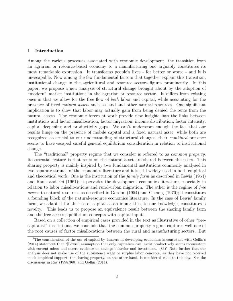
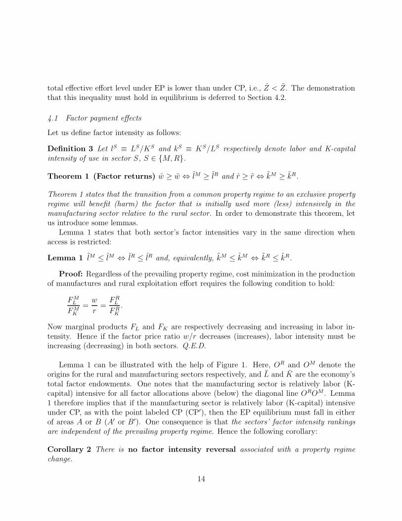
Lemma 1 can be illustrated with the help of Figure 1. Here, OR and OM denote theorigins for the rural and manufacturing sectors respectively, and L and K are the economy’stotal factor endowments. One notes that the manufacturing sector is relatively labor (K-capital) intensive for all factor allocations above (below) the diagonal line OROM . Lemma1 therefore implies that if the manufacturing sector is relatively labor (K-capital) intensiveunder CP, as with the point labeled CP (CP′), then the EP equilibrium must fall in eitherof areas A or B (A′ or B′). One consequence is that the sectors’ factor intensity rankingsare independent of the prevailing property regime. Hence the following corollary:

Corollary 2 There is no factor intensity reversal associated with a property regimechange.

14

✻✛

❄✲

✛ ✲

✻

❄OR

OM

L

K

LM

KMLR

KR

CP

CP′

A

A′

B

B′

EP

EP′

LR

LM

KR KM

Figure 1: Property regimes, factor allocations, and factor intensities

Proof: A reversal of relative factor intensities between sectors implies that equilibria ineach property regime are located on opposite sides of the diagonal line OROM in Figure 1.This violates Lemma 1. Q.E.D.

The following proposition states that when EP is consistent with a drop in rural totaleffective effort as compared to CP, then EP leads to a decreased use of both factors in therural sector.15

Proposition 3 Z < Z ⇔ (LR, KR) ≪ (LR, KR) and, equivalently, (LM , KM) ≫ (LM , KM).

Proof: i) ⇒ Given that Z < Z, then either LR < LR or KR < KR, or both. However,if one factor increases while the other decreases in the rural sector, market clearing impliesthat the opposite happens in the manufacturing sector, which means that factor intensitiesmove in opposite directions, thus violating Lemma 1. Consequently, it must be the casethat LR < LR and KR < KR, and as a result of market clearing, we have LM > LM andKM > KM .

ii) ⇐ is obvious. Q.E.D.

15Note that Lemma 3 does not demonstrate that effective input efforts in the rural sector decrease underEP. This demonstration is deferred to Section 4.2.

15

The following lemma states that if, under CP, the manufacturing sector uses one factormore intensively than the rural sector, then the intensity of use of that factor must be lowerunder EP, and conversely.

Lemma 2 If Z < Z then lM ≥ lR ⇔ lM ≥ lM and, equivalently, kM ≥ kR ⇔ kM ≥ kM .

Proof: i) ⇒ According to Lemma 1, given that lM ≥ lR, as depicted by point CP in Figure1, the new equilibrium with EP must fall strictly within either of areas A or B. Lemma 3,however, rules out area B as a possibility when Z < Z. As a result, the EP equilibrium issuch that lM ≥ lM .

ii) ⇐ a) Begin with the strict inequality lM > lM . According to Lemma 1, we alsohave lR > lR. It is straightforward to verify then that when lM < lR, the preceding twoinequalities imply Z > Z, which we ruled out.

b) In the case of a strict equality lM = lM , Lemma 1 implies lR = lR. Therefore FML = FM

L

and FRL = FR

L . From (5), (9), (8), (16) and (17), this implies that pf ′(Z) = pφ(Z) and thusZ < Z. Suppose now that lM < lR. It is straightforward to verify then that equal factorintensities under both regimes requires that LR = LR and KR = KR, and thus Z = Z. Acontradiction. Q.E.D.

Since a decrease in a factor’s intensity can only come about with an increase in therelative cost of that same factor, we have the following corollary, which we can state withoutproof:

Corollary 3 If Z < Z then lM ≥ lR ⇔ w/r ≥ w/r and, equivalently, kM ≥ kR ⇔ r/w ≥r/w.

The next lemma states that an increase in the use of a factor’s intensity in the manufac-turing sector is associated with a lower return to that factor in equilibrium.

Lemma 3 lM ≤ lM ⇔ w ≥ w and kM ≤ kM ⇔ r ≥ r.

Proof: Observe that w = FML and w = FM

L . Therefore w ≥ w is equivalent to FML ≥ FM

L .Because marginal product FM

L is decreasing in labor intensity, this is also equivalent to

lM ≤ lM . An analogous argument applies to K-capital. Q.E.D.

We can now prove Theorem 1.

Proof of Theorem 1: From Lemma 2, we have lM ≥ lR ⇔ lM ≥ lM . From Lemma 3,the latter inequality is equivalent to w ≥ w. A similar argument applies for K-capital. Q.E.D.

We next turn to the demonstration that the rural total effective effort level will drop inthe transition from common property to exclusive property.

16

4.2 Effective input efforts in the rural sector

In order to demonstrate Theorem 1, we have imposed that the EP regime’s effective effortlevel in the rural sector would be lower than under CP. This may appear like an obviousconsequence of access restriction. However, given that one factor cost is lower under EPthan CP, we cannot a priori rule out the possibility that the net effect will be such that theunit cost of input efforts cR(w, r) drops by so much under EP that the total effective effortexceeds the one under CP. In this section, we show that the total the effective effort underEP is lower than under CP. But beforehand, we establish that the transition from a commonto an exclusive property regime causes a drop in the unit cost of effective effort in the ruralsector, i.e.,

Proposition 4 (effective effort cost reduction) cR(w, r) ≤ cR(w, r).

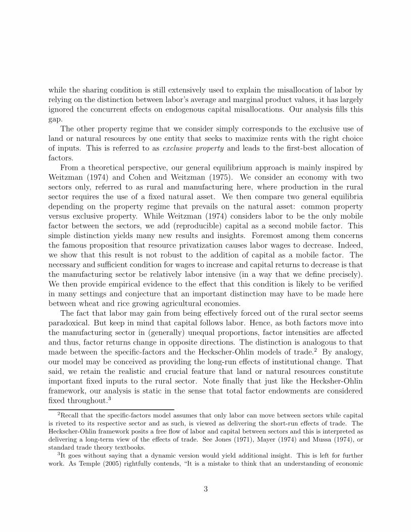
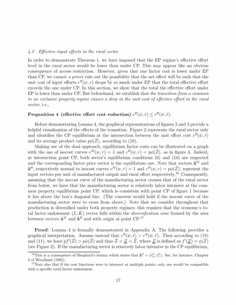
Before demonstrating Lemma 4, the graphical representations of figures 2 and 3 provide ahelpful visualization of the effects of the transition. Figure 2 represents the rural sector onlyand identifies the CP equilibrium at the intersection between the unit effort cost cR(w, r)and its average product value pφ(Z), according to (18).

Making use of the dual approach, equilibrium factor costs can be illustrated on a graphwith the use of isocost curves cM(w, r) = 1 and cR(w, r) = pφ(Z), as in figure 3. Indeed,at intersection point CP, both sector’s equilibrium conditions (6) and (18) are respectedand the corresponding factor price vector is the equilibrium one. Note that vectors aM andaR, respectively normal to isocost curves cM(w, r) = 1 and cR(w, r) = pφ(Z), represent theinput vectors per unit of manufactured output and rural effort respectively.16 Consequently,assuming that the isocost curve of the manufacturing sector crosses that of the rural sectorfrom below, we have that the manufacturing sector is relatively labor intensive at the com-mon property equilibrium point CP, which is consistent with point CP of figure 1 becauseit lies above the box’s diagonal line. (The converse would hold if the isocost curve of themanufacturing sector were to cross from above.) Note that we consider throughout thatproduction is diversified under both property regimes; this requires that the economy’s to-tal factor endowment (L, K) vector falls within the diversification cone formed by the areabetween vectors aM and aR and with origin at point CP.17

Proof: Lemma 4 is formally demonstrated in Appendix A. The following provides agraphical interpretation. Assume instead that cR(w, r) > cR(w, r). Then according to (18)and (11), we have pf ′(Z) > pφ(Z) and thus Z < Z < Z, where Z is defined as f ′(Z) = φ(Z)(see Figure 2). If the manufacturing sector is relatively labor intensive in the CP equilibrium,

16This is a consequence of Shephard’s lemma which states that aS = (cSw, cSr ). See, for instance, Chapter

3 of Woodland (1982).17Note also that if the cost functions were to intersect at multiple points, only one would be compatible

with a specific total factor endowment.

17

✻

✲Z

$

c(w, r)

Z

pφ(Z)

pf ′(Z)

Z

CP

c(w, r)

Z

EP

Figure 2: Rural sector, property regimes, and unit cost of effort

curve cM(w, r) = 1 intersects curve cR(w, r) = pφ(Z) from below (see Figure 3). Now withcR(w, r) > cR(w, r), the rural sector’s unit effort isocost curve under EP must be above thatunder CP; this is illustrated by the dotted curve in Figure 3. The new equilibrium at pointD is characterized by a drop in the relative price of labor and thus a higher intensity in theuse of labor in both sectors. As a consequence, the EP equilibrium falls in region B of Figure1, which corresponds to an increased use of both factors in the rural sector and thereforeZ > Z. A contradiction. Q.E.D.

Proposition 4 implies that the rural sector’s EP regime isocost curve lies below that ofthe CP regime’s. Consequently, the EP equilibrium cost vector (w, r) must be located abovethe CP one (w, r) along the manufacturing sector’s isocost curve, which is consistent withTheorem 1, i.e., in the case where the manufacturing sector is labor intensive under CP,labor (K-capital) is more (less) costly under EP than CP. It also implies that the transitionfrom a common to an exclusive property regime will lead to a contraction of the total effectiveeffort in the rural sector, i.e.,

Proposition 5 Z < Z.

Proof: A formal proof is provided in Appendix B. Graphically, it can be readily verifiedfrom Figure 1 that since the relative cost of labor increases under EP, a lower intensity ofits use in both sectors requires that the EP equilibrium factor allocation must fall into areaA, which is characterized by (LR, KR) ≪ (LR, KR), and therefore Z < Z. Q.E.D.

When combined, propositions 5 and 3 lead us to assert that the transition from a commonto an exclusive property regime will lead to a reallocation of both labor and K-capital fromthe rural sector into the manufacturing sector, thereby causing a contraction of the former

18

✻

✲r

w

CP

cM(w, r) = 1

cR(w, r) = pφ(Z)

aM

aR

D

cR(w, r) = pf ′(Z)

EP

w

rr

w

Figure 3: Isocost curves, property regime equilibria, and factor prices

and an expansion of the latter. This is summarized in the following proposition which westate without proof:

Proposition 6 (Rural factors exodus) (LR, KR) ≪ (LR, KR) and (LM , KM) ≫ (LM , KM)

It is interesting to note that the contraction in the rural sector takes place despite thedrop in the unit cost of the rural effective input effort (proposition 4).

Lemmas 1 and 2 combined with proposition 5 lead us to conclude that if the manufac-turing sector is initially more intensive in one factor, then the transition from a commonproperty regime to an exclusive property regime will cause both sectors to use the other factormore intensively. This result is referred to as factor deepening and stated as follows withoutproof:18

Proposition 7 (Factor deepening) lM ≥ lR ⇔ lM ≥ lM and lR ≥ lR

18Note that factor deepening is defined here as a situation where all sectors of the economy will use onefactor more intensively. It should be contrasted with factor deepening at the aggregate level, which cannotoccur here because total factor endowments are considered fixed.

19

5 Implications and discussions

5.1 Evidence on relative factor intensities

The fact that labor may gain from being denied the rents from the natural capital is a strikingfinding. While the mechanism is now quite clear, the fact that it requires the manufacturingsector to be relatively labor intensive implies that it would still remain a purely theoreticalexercise if this condition were never fulfilled in practice. In this section, we investigate thisempirical question and conclude that it is indeed more than a mere theoretical possibility.To this end, we next propose a representative overview of the relevant empirical literaturewhich lead us to the following three observations: i) In many settings – rich and poor, oldand new – the agricultural sector may quite realistically be more K-capital intensive thanthe non-agricultural sector; ii) There is no general consensus in the literature, not even forthe well-studied case of the US economy; iii) Approaching the question on a case-by-casebasis seems most appropriate.

As discussed in section 2.2, it is first important to dispel the notion that the agriculturaland natural-resource sectors in poorer societies make little use of capital. Indeed, evenwhen the aggregate capital endowments are low and natural assets are held in common,capital may still play a relatively important role. Take the case of sheep farming in medievalEngland. As mentioned in footnote 7, sheep farming is much more capital-intensive than thecultivation of arable land. And though we do not have actual numbers to precisely comparethe capital intensity of pastoral farming with that of the rest of the economy in medievalEngland, one is hard-pressed to imagine many other activities that could have used muchmore capital-intensive techniques of production. We are therefore led to presume that in itsearly stages at least – i.e., before industrialization – the enclosure of the open fields may nothave had the wage depressing effect envisioned in Cohen and Weitzman (1975). Moreover,as Power (1955) argues that England came to dominate the wool trade because of its naturalendowments, there is a suggestion here that whether rural privatization benefits labor ornot may, in the end, largely hinge on an economy’s natural endowments, in support of acase-by-case approach.19 Other rural activities that similarly require a significant amount ofcapital include fishing and tree crop farming.

Turning now to the case of the US economy, the highly cited papers by Valentinyi andHerrendorf (2008) (VH) and Caselli and Coleman (2001) (CC) are representative. Upon di-viding the economy into two sectors only, VH (CC) obtain the factor income shares presentedin Table 1.20

19This may have long-term consequences for an economy in line with Sokoloff and Engerman’s (2000)argument for “... the possibility that initial conditions, or factor endowments broadly conceived, could havehad profound and enduring impacts on long-run paths of institutional and economic development in the NewWorld. (220)”

20Both papers make the explicit distinction between land and reproducible capital incomes. Reproduciblecapital includes structures and equipment for both, while CC additionally includes livestock (as it is based

20

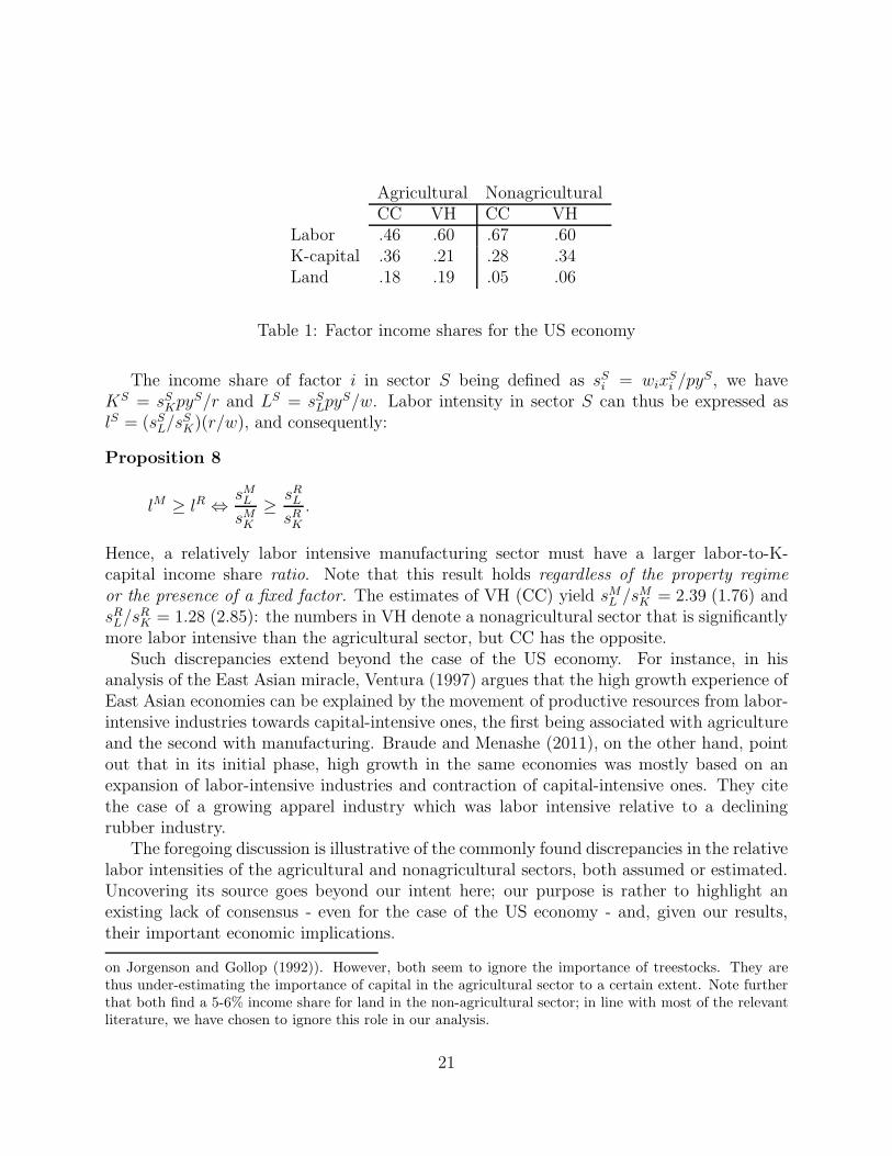
Agricultural NonagriculturalCC VH CC VH

Labor .46 .60 .67 .60K-capital .36 .21 .28 .34Land .18 .19 .05 .06

Table 1: Factor income shares for the US economy

The income share of factor i in sector S being defined as sSi = wixSi /py

S, we haveKS = sSKpy

S/r and LS = sSLpyS/w. Labor intensity in sector S can thus be expressed as

lS = (sSL/sSK)(r/w), and consequently:

Proposition 8

lM ≥ lR ⇔sMLsMK

≥sRLsRK

.

Hence, a relatively labor intensive manufacturing sector must have a larger labor-to-K-capital income share ratio. Note that this result holds regardless of the property regimeor the presence of a fixed factor. The estimates of VH (CC) yield sML /sMK = 2.39 (1.76) andsRL/s

RK = 1.28 (2.85): the numbers in VH denote a nonagricultural sector that is significantly

more labor intensive than the agricultural sector, but CC has the opposite.Such discrepancies extend beyond the case of the US economy. For instance, in his

analysis of the East Asian miracle, Ventura (1997) argues that the high growth experience ofEast Asian economies can be explained by the movement of productive resources from labor-intensive industries towards capital-intensive ones, the first being associated with agricultureand the second with manufacturing. Braude and Menashe (2011), on the other hand, pointout that in its initial phase, high growth in the same economies was mostly based on anexpansion of labor-intensive industries and contraction of capital-intensive ones. They citethe case of a growing apparel industry which was labor intensive relative to a decliningrubber industry.

The foregoing discussion is illustrative of the commonly found discrepancies in the relativelabor intensities of the agricultural and nonagricultural sectors, both assumed or estimated.Uncovering its source goes beyond our intent here; our purpose is rather to highlight anexisting lack of consensus - even for the case of the US economy - and, given our results,their important economic implications.

on Jorgenson and Gollop (1992)). However, both seem to ignore the importance of treestocks. They arethus under-estimating the importance of capital in the agricultural sector to a certain extent. Note furtherthat both find a 5-6% income share for land in the non-agricultural sector; in line with most of the relevantliterature, we have chosen to ignore this role in our analysis.

21

In the case of multi-country studies, Mundlak (2001) is a leading reference on the estima-tion of agricultural production functions at the sectoral level. The author underscores thefact that the assumption of an identical production function for all countries “lacks empiricalsupport” (20), in support of our view that a case-by-case approach may be more suitable. Henonetheless provides pooled estimates of output elasticities for land, labor, and K-capital,and obtains surprisingly high estimates for both land and K-capital. To illustrate, we presentthe more recent (but similar) estimates published in Mundlak et al. (2012) regarding a panelof 30 developed and developing economies. The originality of the approach is that it accountsfor capital of agricultural origin (livestock and treestocks) as well as the usual structures andequipment. They obtain that “The sum of the [output] elasticities of the two types of capitalis 0.46, and the elasticity of land is 0.44. With the sum of the elasticities of 0.90 for capitaland land, there is little scope left for labor and fertilizer” (143). Now given that the standardestimates for the K-capital share of income in the GDP of the average economy is 0.33, suchnumbers would suggest that agriculture is much more K-capital intensive on average.21

Vollrath (2011) similarly considers multiple countries but takes to the letter the propo-sition that agricultural production functions should be estimated separately. He presentsconvincing evidence to the effect that rice production is significantly more labor intensivethan wheat production and argues that this matters when comparing the agricultural sectorsof European countries and rice-growing Asian ones. Given that such differences are valid go-ing back to pre-industrialization times, we can draw implications for a comparative analysisof institutional reform in the rural sectors.

Vollrath (2011) uses CD technologies but does not make the explicit distinction betweenland and K-capital. We therefore adapt our model using CD technologies in order to infer thedistinction. Based on the assumptions made in section 2.2, the agricultural CD productionfunction is Y R = AR(LR)a(KR)bT c, with a+ b+ c = 1. In line with expressions (2) and (3),we have:

Y R = A′Zβ where A′ = ART c and β = 1− c, (19)

Z = (LR)θ(KR)1−θ where θ =a

a+ b. (20)

In the manufacturing sector, we have

Y M = AM(LM )α(KM)1−α. (21)

The labor-elasticity estimates provided in Vollrath (2011) are aE = 0.4 and aA = 0.55,where superscript E and A respectively stand for Europe and “predominantly rice-growing

21Keep in mind that the use of factor income shares as estimators for the parameters of the Cobb-Douglasproduction function requires that all input uses respect the first-order conditions for profit maximization.This is an unrealistic assumption to make for most developing countries as the land and labor markets areoften non-competitive. We understand that it is for this reason that Mundlak (2001) chooses to concentratethe discussion mostly on elasticities.

22

regions of Asia”. Following Table 1, we set the land output elasticity at c = 0.185 forboth regions. We therefore infer the following respective labor elasticities for output (Y R)and effective efforts (Z): bE = 0.415, bA = 0.265, θE = 0.49 and θA = 0.67. As for thenon-agricultural sector, standard labor elasticity estimates are α = 0.66 and are used quiteconsistently for all countries.

We therefore have that while the manufacturing sector is labor-intensive relative to themanufacturing sector in European countries (α > θE), the opposite holds for rice-growingAsian countries (α < θA). Consequently and in accordance with theorem 1, while theadoption of “modern” land market institutions in the rural sector may have tended to raisewages and lower capital returns in Europe, we find the opposite prediction for rice-growingAsian countries. Hence, while Vollrath (2011) shows that differences in agricultural laborintensity help us explain per-capita growth, we have the complementary result that it canalso be useful in explaining income distribution.

5.2 Natural capital, institutions, and productivity analysis

Recently, many growth economists have sought to estimate the extent to which the mis-allocation of workers between the agricultural and the nonagricultural sectors can explainexisting total factor productivity (TFP) differences between countries. To this end, a com-mon method has been to measure the agricultural productivity gap of labor (APGL) whileassuming a CD technology for both sectors.22 In this section, we look at how our analysiscan inform that literature.

The APGL is defined as the ratio of the values of labor’s marginal products (MPL)between the two sectors. Making use of the CD technology introduced in section 5.1, theMPLs are given by MPLM = αY M/LM and MPLR = βθpY R/LR. We thus have:

APGL ≡MPLM

MPLR=

αY M

LM

βθ pY R

LR

(22)

Under a regime of exclusive property, the MPL in each sector being equal to the prevailing

wage rate, we have APGL = 1. Since this corresponds to the efficient allocation of laborbetween the two sectors, the extent of the deviation from unity in the APGL is interpretedas a measure of the severity with which labor is being misallocated between sectors. Nowunder the common property regime, equilibrium condition (16) implies that θpY R/LR = w,and consequently:

APGL =1

β. (23)

22See, for instance, Temple (2005), Vollrath (2009), Adamopoulous and Restuccia (2014), and Gollin et al.(2014b). Note that in this literature generally, the APG implicitly refers to the case of labor misallocationsonly. Given the equally important role that we assign to the misallocation of reproducible capital in ouranalysis, we make the explicit distinction between APGL for labor and APGK for capital.

23

The corresponding calculations for the case of capital yield APGK = 1 and APGK = 1/β.Since β = 1 − c, where c denotes the elasticity of output with respect to natural assets, wehave the following proposition:

Proposition 9 (Natural capital output elasticity and the APG) Under a CP propertyregime in the rural sector, the extent of the misallocation of both labor and reproduciblecapital, if measured by the agricultural productivity gap under Cobb-Douglas technologies, isuniquely determined by the elasticity of output with respect to the natural asset.

This proposition has some interesting implications. Observe first that although the APGsdepend on the importance of the natural asset for production – as per parameter c – theydo not depend on its abundance: land scarcity – say in per capita terms T /L – makes nodifference for the APGs.

Secondly, APG differences between countries can be of two types. If, on the one hand, twocountries use the same production technology, observed differences in the APGs are entirelycaused by property regime differences, and their magnitude increases with the elasticity ofoutput with respect to the natural asset. If, on the other hand, two countries have the sameproperty regime, any observed difference in the APG must be caused by a difference in therural production technology that affects the value of c and the fact that they both have acommon property regime (recall that there is no APG under exclusive property).

6 Conclusion

The existing literature on the general equilibrium effects of agrarian reforms or resourceprivatisation has largely ignored its induced effects on capital flows. To our knowledge, noexisting model allows for the free, endogenous flow of reproducible capital. Yet, one wouldexpect that labor displacements would in turn exert forces on the allocation of capital, atleast in the medium to long run. Our model accounts for these interactions and this yieldsnew results and insights.

We started out by deriving general equilibrium conditions for the allocation of laborand capital under a common property regime in the presence of a fixed factor. Based onthe evidence, we have argued that these conditions may provide a fair representation ofsuch institutions as the sharing family farm, free access to natural resources, tied rents andcollective farming.

We have shown that with mobile capital, the adoption of “modern” market institutionscan raise labor wages and lower capital returns if, and only if, the manufacturing sector isrelatively labor-intensive. Rural reform can therefore have opposite income redistributiveeffects at different times and places. This provides a new mechanism that can help explainthe variety of experiences regarding the redistributive effects of economic development. We

24

have also shown that, under the same condition, the transition can lead to an overall cap-ital deepening of the production processes even though the aggregate capital-labor ratio isunchanged.

Our results highlight the importance of the presence of a fixed natural asset in the ruralsector. Indeed, as this introduces decreasing returns to input efforts, the property regimebecomes relevant. As a consequence, we obtained that the agricultural productivity gaps oflabor and capital are uniquely linked to the output elasticity of land. Since this elasticitymay vary with geography and technology, this also provides a way to explain the observedvariety of productivity gaps.

While our simplified modelling approach was helpful in highlighting some importantforces at play in relation to institutional change, it raises new questions. Some are linked todynamic effects. Indeed, it may be important to consider the presence of stock-flow dynamicsinherent in natural-resource use. In the agricultural sector for instance, much insight couldbe gained with the introduction of biomass soil dynamics in a common property context(Lopez 1997). Dynamic models of aggregate capital deepening (Acemoglu and Guerrieri2008) or differential productivity growths (Alvarez-Cuadrado and Poschke 2011) may inter-act with institutional change and capital mobility in yet unknown manners. Similarly, thedevelopment of transportation facilities between the sectors, as analysed by Adamopoulos(2011), is likely to interact with capital mobility while yielding different result depending onthe property regime.

As we have argued throughout this paper, the use of productive capital in the ruralsector of developing countries can be quite significant. This use is, however, impacted bythe presence of credit constraints, riskiness, and consumption smoothing (Rosenzweig andWolpin 1993; Dercon 1998). Introducing this consideration into our setting seems like anotherpotentially productive avenue of research.

A Proof that cR(w, r) ≤ cR(w, r)

Recall that equilibrium conditions for factor payments must respect condition (6) and eitherof (18) or (11). Let us express those by the following set of two equations, where parameterα is either equal to pφ(Z) or pf ′(Z):

cM(w, r)− 1 = 0, (24)

cR(w, r)− α = 0. (25)

Differentiating these two expressions with respect to parameter α and making use of

25

Cramer’s rule yields:

∂w

∂α=

−cMrcMw cRr − cRwc

Mr

, (26)

∂r

∂α=

cMwcMw cRr − cRwc

Mr

. (27)

Now according to Shephard’s lemma, cSw and cRr denote respectively the quantity of labor andcapital used in sector S per unit of output, i.e., Y ScSw = LS and Y ScSr = KS, S ∈ {M,R}.Inserting this into the above two equations yields:

∂w

∂α=

−Y RKM

LMKR − LRKM, (28)

∂r

∂α=

Y RLM

LMKR − LRKM. (29)

We consequently have:

∂w

∂α< 0 iff lM > lR, (30)

∂r

∂α> 0 iff lM > lR. (31)

Without loss of generality, we posit that lM > lR.23 The above therefore implies that anincrease in α leads to a decrease in w/r.

Assume now that cR(w, r) > cR(w, r). This implies that α must take on a larger valueunder EP than CP and thus, according to the above result, w/r < w/r. But cR(w, r) >cR(w, r) also implies that Z < Z, as can be readily seen from Figure 2. Now according toCorollary 3, lM ≥ lR implies w/r ≥ w/r when Z < Z. A contradiction. Q.E.D.

B Proof that Z < Z

Assume to the contrary that Z ≥ Z. Then, it must be the case that cR(w, r) < cR(w, r).In line with the analysis of Appendix A above, this calls for a lower value of α under EP ascompared to CP and therefore w/r > w/r. Consequently, labor is used less intensively underEP than CP and, as can be readily seen in Figure 1, this requires (LR, KR) ≪ (LR, KR) andthus Z < Z. A contradiction. Q.E.D.

23Note that the problem is undefined for lM = lR.

26

References

Acemoglu, Daron, and Veronica Guerrieri (2008) ‘Capital deepening and nonbalanced eco-nomic growth.’ Journal of Political Economy 116(3), 467–498

Adamopoulos, T., and D. Restuccia (2014) ‘The size distribution of farms and internationalproductivity differences.’ American Economic Review 104, 1667–1697

Adamopoulos, Tasso (2011) ‘Transportation costs, agricultural productivity, and cross-country income differences.’ International Economic Review 52, 489–521

Alvarez-Cuadrado, Francisco, and Markus Poschke (2011) ‘Structural change out of agri-culture: Labor push versus labor pull.’ American Economic Journal: Macroeconomics3, 127–158

Ambec, Stefan, and Louis Hotte (2006) ‘On the redistributive impact of privatizing a resourceunder imperfect enforcement.’ Environment and Development Economics 11, 677–696.mimeo

Anderson, Terry L., and Peter J. Hill (1983) ‘Privatizing the commons: An improvement?’Southern Economic Journal pp. 38–45

Brander, James A., and M. Scott Taylor (1997) ‘International trade and open access re-newable resources: The small open economy case.’ Canadian Journal of EconomicsXXX(3), 526–552

Braude, Jacob, and Yigal Menashe (2011) ‘The asian miracle: Was it a capital-intensivestructural change?’ The Journal of International Trade and Economic Development20(1), 31–51

Brito, Dagobert L., Michael D. Intriligator, and Eytan Sheshinski (1997) ‘Privatization andthe distribution of income in the commons.’ Journal of Public Economics 64, 181–205

Brooks, Michael A., and Ben J. Heijdra (1990) ‘Rent-seeking and the privatization of thecommons.’ European Journal of Political Economy 6, 41–59

Carter, Michael R. (1984) ‘Resource allocation and use under collective rights and labourmanagement in peruvian coastal agriculture.’ Economic Journal

Caselli, Francesco (2005) ‘Accounting for cross-country income differences.’ In Handbookof Economic Growth, ed. Philippe Aghion and Steven N. Durlauf, vol. 1A (Elsevier)chapter 9, pp. 679–741

27

Caselli, Francesco, andWilbur John Coleman II (2001) ‘The us structural transformation andregional convergence: A reinterpretation.’ Journal of Political Economy 109(3), 584–616

Chernina, Eugenia, Paul Castaneda Dower, and Andrei Markevich (2014) ‘Property rights,land liquidity, and internal migration.’ Journal of Development Economics

Cheung, Steven N. S. (1970) ‘The structure of a contract and the theory of a non-exclusiveresource.’ Journal of Law and Economics XIII, 45–70

Chichilnisky, Graciela (1994) ‘North-south trade and the global environment.’ The AmericanEconomic Review 84(4), 851–874

Cohen, Jon S., and Martin L. Weitzman (1975) ‘A marxian model of enclosures.’ Journal ofDevelopment Economics 1, 287–336

Corden, W. M., and R. Findlay (1975) ‘Urban unemployment, intersectoral capital mobilityand development policy.’ Economica 42(165), 59–78

de Meza, David, and J.R. Gould (1987) ‘Free access versus private property in a resource:Income distributions compared.’ Journal of Political Economy 95(6), 1317–1325

Demsetz, Harold (1967) ‘Toward a theory of property rights.’ American Economic Review57, 347–359

Dercon, Stefan (1998) ‘Wealth, risk and activity choice: cattle in western tanzania.’ Journalof Development Economics 55, 1–42

Drazen, Allan, and Zvi Eckstein (1988) ‘On the organization of rural markets and the processof economic development.’ American Economic Review 78, 431–443

Fafchamps, Marcel (1998) ‘The tragedy of the commons, livestock cycles and sustainability.’Journal of African Economies 7(3), 384–423

Foster, Andrew D., and Mark R. Rosenzweig (2008) ‘Economic development and the de-cline of agricultural employment.’ In Handbook of Development Economics, ed. T. PaulSchultz and John A. Strauss, vol. 4 (Elsevier B.V.) chapter 47, pp. 3051–3083

Gollin, Douglas (2014) ‘The lewis model: A 60-year retrospective.’ Journal of EconomicPerspectives 28, 71–88

Gollin, Douglas, David Lagakos, and Michael E. Waugh (2014a) ‘Agricultural productiv-ity differences across countries.’ American Economic Review: Papers and Proceedings104, 165–170

28

(2014b) ‘The agricultural productivity gap.’ The Quarterly Journal of Economics

Gordon, H. Scott (1954) ‘The economic theory of a common-property resource: The fishery.’Journal of Political Economy VXII, 124–142

Harris, John R., and Michael P. Todaro (1970) ‘Migration, unemployment and developmnent:A two-sector analysis.’ American Economic Review 60, 126–142

Hotte, Louis, Ngo Van Long, and Huilan Tian (2000) ‘International trade with endogenousenforcement of property rights.’ Journal of Development Economics 62, 25–54

Jarvis, Lovell S. (1974) ‘Cattle as capital goods and ranchers as portfolio managers: Anapplication to the argentine cattle sector.’ Journal of Political Economy 82, 489–520

Jones, R. W. (1971) ‘A three factor model in theory, trade and history.’ In Trade, Balanceof Payments, and Growth, ed. J. Bhagwati, R.W. Jones, R. Mundell, and J. Vanek(Amsterdam: North-Holland)

Jorgenson, Dale W., and Frank M. Gollop (1992) ‘Productivity growth in u.s. agriculture:A postwar perspective.’ American Journal of Agricultural Economics 74(3), 745–750

Karp, Larry (2005) ‘Property rights, mobile capital, and comparative advantage.’ Journalof development economics 77, 367–387

Lewis, Arthur (1954) ‘Economic development with unlimited supplies of labor.’ The Manch-ester School 22, 139–192

Lopez, Ramon (1997) ‘Environmental externalities in traditional agriculture and the impactof trade liberalization: The case of ghana.’ Journal of Development Economics 53, 17–39

Lucas, Robert E.B. (1997) ‘Internal migration in developing countries.’ In Handbook of Pop-ulation and Family Economics, ed. M.R. Rosenzweig and O. Stark, vol. 1 (ElsevierScience) chapter 13, pp. 721–798

Mathijs, Erik, and Johan F. M. Swinnen (1998) ‘The economics of agricultural decollec-tivization in east central europe and the former soviet union.’ Economic Developmentand Cultural Change 47(1), 1–26

Mayer, Wolfgang (1974) ‘Short-run and long-run equilibrium for a small open economy.’Journal of Political Economy 82, 955–967

Mundlak, Yair (2001) ‘Production and supply.’ In Handbook of Agricultural Economics, ed.B. Gardner and G. Rausser, vol. 1 (Elsevier Science) chapter 1, pp. 3–85

29

Mundlak, Yair, Rita Butzer, and Donald F. Larson (2012) ‘Heterogeneous technology andpanel data: The case of the agricultural production function.’ Journal of DevelopmentEconomics pp. 139–149

Munshi, Kaivan, and Mark Rosenzweig (2016) ‘Networks and misallocation: Insurance, mi-gration, and the rural-urban wage gap.’ American Economic Review

Mussa, Michael (1974) ‘Tariffs and the distribution of income: The importance of factorspecificity, substitutability, and intensity in the short and long run.’ Journal of PoliticalEconomy 82, 1191–1204

Power, Eileen (1955) The wool trade in English medieval history, being the Ford lectures(London: Oxford University Press)

Ranis, Gustav, and John C. H. Fei (1961) ‘A theory of economic development.’ AmericanEconomic Review 51, 533–565

Ray, Debraj (1998) Development Economics (Princeton University Press)

Restuccia, Diego, Dennis Tao Yang, and Xiaodong Zhu (2008) ‘Agriculture and aggregateproductivity: A quantitative analysis.’ Journal of Monetary Economics pp. 234–250

Roemer, John E. (2015) ‘Kantian optimization: A microfoundation for cooperation.’ Journalof Public Economic pp. 45–57

Rosen, Sherwin, Kevin M. Murphy, and Jose A. Scheinkman (1994) ‘Cattle cycles.’ Journalof Political Economy 102(3), 468–492

Rosenzweig, Mark R., and Kenneth I. Wolpin (1993) ‘Credit market constraints, consumptionsmoothing, and the accumulation of durable production assets in low-income countries:Investments in bullocks in india.’ Journal of Political Economy 101, 223–244

Temple, Jonathan (2005) ‘Dual economy models: A primer for growth economists.’ TheManchester School 73(4), 435–478

Temple, Jonathan, and Ludger Wossmann (2006) ‘Dualism and cross-country growth regres-sions.’ Journal of Economic Growth 11, 187–228

Valentinyi, Akos, and Berthold Herrendorf (2008) ‘Measuring factor income shares at thesectoral level.’ Review of Economic Dynamics

Ventura, Jaume (1997) ‘Growth and interdependence.’ Quarterly Journal of Economics112, 57–84

30

Vollrath, Dietrich (2009) ‘How important are dual economy effects for aggregate productiv-ity?’ Journal of Development Economics 88, 325–334

(2011) ‘The agricultural basis of comparative development.’ Journal of Econmic Growth16, 343–370

Weitzman, Martin L. (1974) ‘Free access vs private ownership as alternative systems formanaging common property.’ Journal of Economic Theory 8, 225–234

Woodland, A.D. (1982) International Trade and Resource Allocation (Amsterdam: North-Holland Publishing Company)

Young, Alwyn (2013) ‘Inequality, the urban-rural gap and migration.’ The Quarterly Journalof Economics

Zhao, Xiaoxue (2015) ‘To reallocate or not? optimal land institutions under communaltenure: Evidence from china.’ Working Paper, Duke University, May

31