Board of Governors of the Federal Reserve System International Finance Discussion Papers

Number 1071 December 2012

Institutional Herding in the Corporate Bond Market

Fang Cai, Song Han, and Dan Li

NOTE: International Finance Discussion Papers are preliminary materials circulated to stimulate discussion and critical comment. References to International Finance Discussion Papers (other than an acknowledgment that the writer has had access to unpublished material) should be cleared with the author or authors. Recent IFDPs are available on the Web at www.federalreserve.gov/pubs/ifdp/. This paper can be downloaded without charge from the Social Science Research Network electronic library at www.ssrn.com.

Institutional Herding in the Corporate Bond Market*

Fang Cai, Song Han, and Dan Li * Abstract: We find substantial herding in U.S. corporate bonds among bond fund managers, much higher than that previously documented for the equity market. Herding is generally stronger among illiquid bonds, and buy herding and sell herding are driven by different factors. In particular, sell herding increases on negative news about bond ratings and corporate earnings. Interestingly, increases in ex-post transparency in corporate bond trading through Trade Reporting and Compliance Engine (TRACE) led to higher buy herding but not to higher sell herding. Finally, we find significant return reversals in the post-herding quarters, especially for sell herding and for junk bonds. Price reversal is most prominent when funds herd to sell illiquid bonds, which suggests that temporary price pressure is the reason behind price reversal. Keywords: corporate bond, herding, liquidity, institutional investors JEL classifications: F21, G11, G14, G15

* The authors are staff economists at the Board of Governors of the Federal Reserve System, Washington, D.C. 20551 U.S.A. The views in this paper are solely the responsibility of the authors and should not be interpreted as reflecting the views of the Board of Governors of the Federal Reserve System or of any other person associated with the Federal Reserve System. Weina Zhang and participants of the China International Conference of Finance and the seminar at the Federal Reserve Board. Corresponding author: Fang Cai, fang.cai@frb.gov, or (202)452-3540.

2

1. Introduction

The market for the U.S. corporate bonds is large and dominated by institutional

investors. As of the end of 2010, institutional investors held about three quarters of the

$7.5 billion outstanding corporate bonds issued by U.S. firms.1 In addition, institutional

trades account for most of the dollar trading volume of corporate bonds (Edwards, Harris,

and Piwowar (2007)). Thus, understanding the trading behavior of institutional investors

and its effects on the informational efficiency is critical for asset valuation, risk

management, and policy making regarding the corporate bond market.

In this paper, we study trading of U.S. corporate bonds by institutional investors

with a focus on institutional herding. By definition, institutional herding is a trading

pattern where institutional investors buy or sell the same set of securities at the same time.

Herding has been commonly regarded as a key characteristic of institutional trading. In

particular, critics have been concerned about the possible destabilizing effects of herding

on securities prices.2 Institutional herding has been subjected to extensive studies in

financial economics. Most of these studies, however, focus on the equity markets and

report that institutional herding is very low in general, and moderate for only some

segments of the markets with relatively low liquidity or information transparency (see,

e.g., Lakonishok, Shleifer, and Vishny (henceforth LSV, 1992), Froot, Scharfstein, and

Stein (1992), Hirshleifer, Subrahmanyam, and Titman (1994), Wermers (1999), and

Hirshleifer and Teoh (2003)). The dynamics of post-herding returns is also widely

studied and the findings are more controversial. While Nofsinger and Sias (1999),

1Estimates based on data from the Flow of Funds Accounts of the United States. 2 For example, a pension fund manager said, “institutions are herding animals. We watch the same indicators and listen to the same prognostications. Like lemmings, we tend to move in the same direction at the same time. And that naturally, exacerbates price movements” (Lowenstein and Donnelly (1989)).

3

Wermers (1999), and Sias (2004) provide evidence that asset prices continue in the direction

of the herd during subsequent periods, more recent studies such as Sharma, Easterwood and

Kumar (2006), Brown, Wei, and Wermers (2009), Dasgupta, Prat and Verardo (2007),

San (2007) and Puckett and Yan (2009) all find evidence of return reversals following

intense institutional trading.

The market for corporate bonds provides a unique laboratory to broaden our

understanding of the trading behavior by institutional investors. Unlike the markets with

organized exchanges—the focus of previous studies—corporate bonds are mostly traded

in the over-the-counter (OTC) markets. Because OTC markets are generally viewed to

have low liquidity and high information asymmetry, the results of existing studies

suggest that herding may be more significant in the corporate bond markets.

Combining a comprehensive dataset on U.S. corporate bond holdings by

institutional investors and the corporate bond transaction data from the Trade Reporting

and Compliance Engine (TRACE), we analyze the following. First, we estimate the

extent of institutional herding in trading U.S. corporate bonds. We adopt the herding

measures proposed by Lakonishok, Shleifer, and Vishny (henceforth LSV, 1992),

following the existing literature. In essence, the LSV measure estimates the unusually

correlated trades of certain securities among a group of investors. We find substantial

institutional herding in U.S. corporate bonds, much higher than that previously

documented in the equity markets.

Second, we examine what factors drive institutional herding in the corporate bond

market. We show that buy herding and sell herding are driven by different factors. In

particular, sell herding increases on negative news about bond ratings and corporate

earnings. Herding is stronger in bonds that are smaller, lower-rated, with higher

4

information asymmetry. We also find that mimicry is an important factor driving

institutional herding in the bond market. Mimicry is manifested in two ways. First, we

find that within a quarter, buy herding increases with post-trade transparency, i.e.,

following the dissemination of trade information by TRACE, buy herding increases

significantly. Second we find that over quarters, there is a strong correlation between

current trading and past trading of others.

Finally, we analyze the dynamics of the post-herding returns to investigate

whether institutional herding stabilizes or destabilizes bond prices. We find significant

return reversals in the post-herding trades, especially for sell herding. This finding

suggests that sell herding in the U.S. corporate bond market destabilizes bond prices.

Price reversal is most prominent when funds herd to sell illiquid bonds, which suggests

that temporary price pressure is the reason behind price reversal.

Our main contributions to the literature are the following. First, we fill in the void

in the literature on institutional herding and its price impact with fresh evidence from the

OTC market. As LSV argued, the low herding behavior in the equity market is in sharp

contrast with anecdotal overservations, but it may be explained by the heterogeneity in

trading strategies in the stock market and the fast speed with which price reflects private

information (see also Wermer (2009) and others). As suggested by these studies,

herding may be more prevalent and have larger price impact in markets with low liquidity

and more opaqueness. Our results confirm such conjectures.

Second, we identify some important factors that drive institutional herding in the

corporate bond market, and thus we help assess the empirical significance of alternative

theories on herding.

5

Some existing theories explaining why institutional investors might herd suggest

that institutions may trade together simply because they receive correlated private

information, perhaps from analyzing the same indicators (see Froot, Scharfstein, and

Stein (1992) and Hirshleifer, Subrahmanyam, and Titman (1994)). or share some

common preferences for securities with certain characteristics, such as liquid, high

volatility and high visibility stocks (Falkenstein (1996)). Other studies suggest that

institutional investors may infer private information from the prior trades of better-

informed institutions and trade in the same direction (Bikhchandani, Hirshleifer, and

Welch 1992)). In doing so, they may disregard their private information and trade with

the crowd due to the reputational risk of acting differently from other managers

(Scharfstein and Stein (1990)). We find strong evidence of mimicry behavior among

institutional investors, which supports the second strand of the literature.

Third, we study the dynamics of post-herding returns and provide new evidence

of the price impact of institutional herding onbond prices. The empirical evidence on the

price impact of institutional herding has been mixed. On one hand, Nofsinger and Sias

(1999), Wermers (1999), and Sias (2004) all provide evidence that asset prices continue

in the direction of the herd during subsequent periods, suggesting that herding may be

allow markets to impound new information into asset prices more quickly than otherwise.

On the other hand, more recent studies such as Sharma, Easterwood and Kumar (2006),

Brown, Wei, and Wermers (2009), Puckett and Yan (2009), and Dasgupta, Prat and

Verardo (2011) all find evidence of return reversals following intense institutional

herding, consistent with the view that herding may drive security prices beyond

fundamental values, resulting in overshooting and subsequent return reversals. We find

6

that buy herding and sell herding have asymmetric price impact, and the return reversal

following sell herding suggests that sell herding is price destabilizing. Moreover, the

return reversal is mostly driven by bonds that are highly illiquid, suggesting temporary

price pressure from concerted sell effort by various funds is the reason of price reversal.

The rest of the paper is organized as follows. Section 2 describes the data,

sampling, and our construction of herding measures; Section 3 presents empirical results;

and Section 4 concludes.

2. Data, Sampling, and Herding Measures

2.1. Data

We construct our data from several sources. We obtain data on corporate bond

holdings by institutional investors from the Thompson Reuters/Lipper eMaxx fixed

income database (Lipper data). The data contain details of quarterly holdings of a wide

range of fixed income securities by U.S. and European insurance companies, U.S.,

Canadian and European mutual funds, and leading U.S. public pension funds.3 We refer

these institution investors generally as “funds” throughout the paper.

For the bonds in the Lipper data, we obtain information from the Fixed

Investment Securities Database (FISD) on bond characteristics, including issuance date,

maturity date, amount outstanding, and rating history. For the pricing information of

these bonds, we use data from Merrill Lynch’s Corporate Bond Index Database (“the ML

data”). The ML data contain daily prices and a limited number of other variables, such as

3 According to Lipper, holdings by insurance companies come from insurance company reports to National Association of Insurance Commissioners (NAIC). Mutual fund holdings are reported on Securities and Exchange Commission (SEC)’s form N-CSR as required by Section 30(b)(2) of the Investment Company Act of 1940 (the “Act”) and Section 13(a) or 15(d) of the Securities Exchange Act of 1934 (the “Exchange Act”). Holdings by pension funds etc. are collected on solicitation basis.

7

accrued interests and credit rating, on a representative pool of rated U.S. public corporate

bonds. The ML bond prices are bids of major dealer quotes. The main advantage of

using the ML data, instead of transactions data, for the bond pricing information is that

they allow for a relatively balanced sample back to 2003, when the transactions data were

very thin.

For our analysis, we also obtain corporate bond trading information from TRACE.

Until recently, information about corporate bond trading activity was not widely available

to the public. Under pressure from regulatory agencies and investors, the Financial

Industry Regulatory Authority (FINRA) now requires its members to report their

secondary market transactions, including price and trade quantity, to TRACE. We use

TRACE for the following purposes: First, we use the transaction information to estimate

bond liquidity. Second, we use the TRACE phase-in dissemination as a natural

experiment to study the effect of trade-transparency on institutional herding. Third, we

use TRACE as an alternative data for the bond pricing information to study the

robustness of our main results.

2.2. Sampling

We focus on U.S. dollar-denominated public corporate bonds reported in the

Lipper data.4 Also, we restrict our sample to bonds with complete information from

FDIC regarding date of issuance, maturity, and amount outstanding, and with fixed

coupons. These filters result in 22,832 unique bonds. We then exclude bonds that are

either labeled as "private placement bonds" or labeled as "Rule-144a". This left us with

4 Private bonds account for 35 percent of the overall Lipper data. We find that herding among private bonds are much higher than public bonds, possibly due to the lack of information transparency and high trading costs.

8

18,633 unique bonds. Finally, we exclude bonds with age less than 3 quarters—as these

newly issuance bonds may still be in the distribution process—and bonds with remaining

maturity less than 2 quarter—as these bonds either automatically disappear from an

investor’s portfolio or were traded out just before maturity. As a result of these

additional filters, our analysis sample consists of 17,771 unique CUSIPs by 4,152 issuers

(identified by the first 6 digits of CUSIPs) with 197,226 bond-quarter records and

5,723,469 bond –fund-quarter records. On average (over all bond-quarters), the bonds

have 8.8 years remaining to maturity, are 5.5 years since issuance, have $272 million

outstanding, and about 79 percent of them are investment-grade bonds. In terms of

coverage of the holding information reported in the Lipper data, the total holding by U.S.

funds accounts for about 35 percent of the par amount of of the outstanding amount of the

same universe of bonds, as shown in Panel B of Table 1. The holding by foreign funds

accounts for only less than 1 percent of total outstanding amount, in part because holding

reporting by foreign funds is mostly voluntary.

2.3. Herding Measures

Following the existing literature, we adopt the herding measure proposed by

Lakonishok, Shleifer, and Vishny (1992; henceforth “the LSV measure”) as our working

horse (e.g., Grinblatt, Titman, and Wermers, 1995; Wermers, 1999). We estimate the LSV

measure for each bond-quarter, by defining that a fund buy (sell) a bond in a quarter if the

fund reports to have increased (decreased) its holding of the bond in the quarter.5

Specifically, the LSV measure for bond i in quarter t is calculated as:

HMit = |pit − E(pit)| − E(|pit − E(pit)|) (1)

5 Due to data limitations, we have to infer net trades from change of quarterly holdings.

9

where #

# #it

itit it

Buyp

Buy Sell

, or the proportion of all trades in bond i during quarter t that

are buys. We use market average buy intensity pt to proxy for the expected level of buy

intensity for each bond, E(pit). That is,

#

# #

iti

it t

it iti i

BuyE p p

Buy Sell

The last term in (1), E(|pit − E(pit)|), is often referred to as the adjustment factor,

accounting for the fact that the first term in (1), which is an absolute value, is always greater

than zero. The adjustment makes it possible to make direct comparison across bonds or over

time. The adjustment factor is calculated under the null hypothesis that #Buyit follows a

binomial distribution with parameters pt and Nit = #Buyit + #Sellit. The LSV herding

measure can be computed at the level of all funds or a subgroup of funds. For a given

group of funds, the adjustment factor E(|pit − E(pit)|) and proxy of E(pit) are based on

trading within only that group.

The herding measure essentially tests whether the observed distribution of pit is

fat-tailed relative to the expected distribution under the null hypothesis that, conditional

on the overall observed level of buying E(pit), trading decisions across funds are

independent. Values of HMit that are significantly different from zero are interpreted as

evidence of herd behavior.6 To ensure that our estimated herding measure behaves

reasonably well statistically, we restrict our sample to bond-quarters with the bond traded

by at least five funds in the quarter.

6 The drawback of the LSV measure is that it does not utilize information regarding size of trades. It also does not retain fund-specific information after aggregation, which makes it difficult to analyze inter-temporal trading strategies of each fund.

10

The above LSV measure does not distinguish herding by trading directions. To

make such differentiation, we follow Wermers (1999) to estimate a herding measure each

for buy and sell herding separately. Specifically,

BHMit = HMit| pit > E(pit), (2)

SHMit = HMit| pit < E(pit). (3)

That is, when the observed buy frequency is greater (less) than expected buy frequency,

the LSV measure is buy (sell) herding measure, BHM (SHM).

3. Empirical Results

In this section, we first present our estimated results on the levels of institutional

herding in the corporate bond trading. We examine the overall herding levels as well as

herdings along some key aspects of bond characteristics as motivated by the existing

literature. We then present our regression results on the determinants of institutional

herding. In particular, we explore if institutional herding in corporate bonds is driven by

mimicry motives. Finally, we show our results on return reversals based on a portfolio

approach, from which we infer the price impact of institutional herding in the corporate

bond market.

3.1 Levels of Institutional Herding

Panel A of Table 2 presents the levels of herding measured in terms of HM, BHM,

SHM at the fund level. The following patterns stand out. First, the level of herding in

the corporate bonds are substantially higher than that reported for stocks, even that for

small stocks on which herding may be the strongest. The average corporate bond herding

11

measure is about 0.15, while stock herding measures were found to generally under 0.04

in the literature (e.g., LSV (1992), Wermers (1999)). These studies also find that even

for small stocks—the group of stocks on which herding is the strongest, the herding

values are only around 0.06. The stronger herding in the corporate bond market is

consistent with the view that information acquisition and trading are more costly in the

OTC market due to its opaqueness, making it more desirable to free ride on other

instititutions’ information acquisition through herding.

Second, herding is significantly stronger on the sell-side than on the buy-side. As

we can see, the average sell-herding measure is 0.10, slightly higher than the average

buy-herding measure 0.09. The asymmetry between sell and buy herding is also found in

previous studies, but only for small stocks (e.g., Werners (1999)). Also, the levels of

both buy and sell herdings are substantially stronger in the corporate bond market than

their counterparts even for small stocks.

The above two findings are not all due to correlated trading by funds within the

same fund family. Funds within a fund family may trade correlatively because they may

be affected by some common factors related to the family. To address this concern, we

re-estimate the herding measures for each bond-quarter by counting a trade as the change

in total holdings of a bond by all funds within a fund family. As shown in Panel B of

Table 2, the levels of herding estimated using aggregate trading at the fund family level

are lower than those estimated at the fund level. However, the magnitude of overall

herding remains fairly large, and the asymmetry between sell and buy herdings continues

to hold.

12

Our results are also robust to taking into account multiple bonds issued by the

same issuer. In contrast to stocks, an issuer often has multiple bonds outstanding at the

same time. So one may be concerned that herding measures may be affected if a fund

sells or buys all bonds of the same issuer at the same time. To address such concern, we

re-estimated herding measures by counting a trade as any change in a fund’s total

holdings of all bonds from a single issuer (issuer is identified by the first 6 digits of bond

CUSIPs). As shown in Panel C of Table 2, the results on the magnitude of herding as

well as the asymmetry between sell and buy herding remain similar. We show similar

herding panel by fund type in Panel D.

3.2 Herding and Bond Characteristics

To determine if there is any cross-sectional difference in bond herding, we

examine bivariate relationship between herding measures and several bond characteristics.

Results are shown in Table 3. Panel A shows herding measure by bond age and life to

maturity. Buy herding is stronger in newly issued bonds, while sell herding is stronger in

bonds about to mature. Panel B shows herding measure by size. We find that herding is

decreasing in the bond size variable, consistent with the finding in existing studies that

herding is significantly stronger among small stocks. Panel C shows that herding is

stronger in bonds with lower rating, especially junk bonds. Panel D shows that herding

measure is not significantly related to the liquidity measure (liquidityis defined here as

the principle component of three alternative liquidity measures that are discussed in the

appendix, LiqAmd, LiqRoll, or LiqIQR).

13

The relationship between herding and bond liquidity seems to be U-shaped rather

than monotonic. Herding is highest among most illiquid bonds, but also high among

bonds that are most liquid. The U-shaped relationship between liquidity and herding is

interesting, as it likely mirrors the trade-off between the benefit from information based

herding and the transaction cost of herding. On the one hand, trades on illiquid bonds are

more likely to contain more private information, and making herding a more effective

trading stragegy, on the other, illiquid bonds are more costly to trade, making the strategy

less profitable. Thus, only very liquid bonds (low transaction cost) or very illiquid bonds

(high private information) are herded upon.

3.3 Determinants of Herding

To provide a more comprehensive view, we use a regression approach to analyze

the importance of a number of factors in explaining the cross-sectional variations in

institutional herding. Motivated by existing studies, we consider the following

explanatory variables. First, we include a set of bond characteristics as the independent

variables in our regressions:

The logarithm of bond age (log(age))

Current credit rating (average rating across three rating agencies, with a higher

number denoting a lower credit rating. AAA = 1, AA1(AA+) = 2, …)

A dummy variable that equals 1 to indicate investment grade bond (Investment

Grade)

The logarithm of bond par amount at issuance (logpar)

Bond liquidity as defined in Section 3.2

14

We also use lagged abnormal return as a control variable to account for momentum

effect. Abnormal bond return (ari,t) is calculated as a bond i’s total return during the

quarter t (tri,t) subtracted by the par-weighted average return of the pool of bonds ( ,p ttr )

that share similar time to maturity, credit ratings and financial/nonfinancial

classification,7 where

, , , , , , , ,,

, , , ,

( ) ( ) * *(1 ) ti t end i t end i t begin i t begin coupon payment Libor

i ti t begin i t begin

p AI p AI I C rtr

p AI

,

in which AI denotes accrued interest and Icoupon is an indicator whether coupon payment

(Cpayment) occurs during quarter t.8

Second, we include two variables indicating the arrival of public news: change of

credit rating from last quarter (∆ratingt-1, where a positive rating change corresponds to a

downgrade) and earnings surprises in last quarter. As discussed earlier, herding may be

driven by correlated information, such as the arrival of public news. Rating changes

(∆ratingt-1) is the difference of our numerical rating variable, with a positive rating

change corresponding to a downgrade. Earnings surprises are estimated using

information from the I/B/E/S data for each bond-issuing firm over the sample period. In

particular, we follow the literature to use standardized surprise, (Ait – Eit)/σi, where Ait is

the announced earnings per share of firm i in quarter t, Eit is the median earnings forecast

by equity analysts, and σi is the time series standard deviation of the forecast error.

Finally, we also examine the role of information asymmetry in institutional

herding. Theoretical models of Avery and Zemsky (1998) and Bikhchandani, Hirshlefier,

7 We also use simple average return in robustness check and the results are qualitatively similar. 8 we use the ML data as our main source for bond pricing information, but repeat our analysis using TRACE as the alternative pricing source and yield similar results.

15

and Welch (1992) suggest that higher information asymmetry may lead to greater herding.

We use the probability of information-based trading (PIN) proposed by Easley, Hvidkjaer,

and O’Hara (2002) as a proxy for information asymmetry in bond trading. Using the

trade direction variable in our TRACE data, we estimate the PIN model for each bond-

quarter through a maximum likelihood method.

Summary statistics for bond characteristics, liquidity measures, rating changes

and earning surprises are presented in Table 4.

Table 5 shows the regression results of institutional buy herding and sell herding

using the Fama-MacBeth regression approach on the quarterly samples.

The main findings from the regressions are the following. First, herding is

significantly related to bond characteristics such as bond size, age, and credit risk; but the

effects differ for buy herding from sell herding. Other things being equal buy herding is

more pronounced in small bonds than in large bonds. This result is consistent with LSV

(1992) and Wermers (1999) that stock herding is found mainly in small stocks. However,

sell herding does not seem to be significantly related to bond size. The effect of bond age

on herding is also significant, but it differs for buy and sell herding. Buy herding occurs

more in newer bonds while sell herding is usually seen in more seasoned bonds. Note

that this result is not driven by newly issued bonds or bonds is about to about mature as

we have excluded bonds that were issued in past two quarters and bonds that one quarter

to mature. The effect of credit rating also differs for buy and sell herding. Buy herding

does not vary with credit rating, but sell herding varies strongly with credit rating, with

stronger sell herding among bonds with higher credit risk. In addition, sell herding is

16

significantly stronger in speculative-grade bonds than in investment-grade bonds, but

such nonlinear effect is not statistically significant for buy herding.9

Second, sell herding, but not buy herding, is stronger in bonds with higher

information asymmetry, which suggests that sell herding is more likely driven by

information cascade, as in Avery and Zemsky (1998) and Bikhchandani, Hirshlefier, and

Welch (1992) In addition, the coefficients on the bond liquidity variableare all

statistically insignificant for both buy and sell herding regressions. These results are not

surprising, given the U-shaped relationship between liquidity and herding as shown in

Table 3.

Third, we find asymmetric responses of buy and sell herding to public news.

Other things being equal, sell herding by institutions are more pronounced in bonds with

recent downgrades and negative earnings surprises, while rating and earnings news does

not affect buy herding. This result is consistent with previous studies that bond investors

use generally buy-and-hold strategies and bias to sell when there is bad news on a bond’s

credit risk (e.g., Jostova, Nikolova, Philipov and Stahel (2010)). Finally, we don’t find

herding to be driven by past returns. The coefficients on the lagged abnormal returns are

not significant.

3.4 Herding and Transparency

As discussed above, the high liquidity cost and information asymmetry may cause

investors to imitate trading behaviors of other investors in order to lower their cost of

information collection. To further examine the mimicry motive of herding, we analyze

9 Nonlinear bond payoffs are also found at rating changes (Jorion and Zhang (2007)) and earnings announcements (Easton, Monahan, and Vasvari (2009)).

17

the effect of increased trading transparency in the corporate bond market on institutional

herding. After all, for imitative trading to occur, trading or holdings of other investors

must be observable. Such observability issue has largely been overlooked in the existing

studies. Here we use the phasing-in dissemination of TRACE data as a natural

experiment to study the effect of trading transparency on institutional herding.

Since the inception of TRACE on July 1, 2002, FINRA has increased the trading

transparency of corporate bonds by phasing in real-time dissemination of the reported

trading information to the public. Phase I of the public dissemination took place on July

1st, 2002 for a small number of selected corporate bonds. Phase II occurred in March

and April of 2003, extending real-time dissemination to about 5000 bonds. Phase III

occurred in two steps on October 4, 2004 and February 7, 2005, expanding to the OTC

trades of all but Rule 144A corporate bonds. Our focus is the effect of the last phase-in

dissemination on institutional herding as the phase happened during our sample period.

We use a difference-in-difference approach in our analysis. To do so, we define

two dummy variables: one indicating whether the bonds are included in the Phase III of

the real-time dissemination (“Phase III bonds”, equal to 1 if a bond is added to

dissemination in Phase III, 0 otherwise), and the other indicating whether the quarter is

after the completion of Phase III (“Post Phase III”, equal to 1 if after the first quarter of

2005). We exclude the periods of the fourth quarter of 2004 and the first quarter of 2005

from our regressions because the two consecutive quarters are transitional periods for the

last phase. We regress our herding measures on bond characteristics, rating change,

earnings surprise, and lagged abnormal returns as well as “Phase III bonds”, “Post Phase

III”, and the interactive term of these two dummies. In addition, we include a dummy

18

variable “Phase II bonds” to indicate whether a bond has been included in Phase II of the

public dissemination, which occurred before the starting quarter of our sample period.

This last dummy variable is to control for the bonds in our sample that have not ever been

included by FINRA as eligible for TRACE reporting or dissemination, We don’t include

any liquidity variables or PIN because these variables are missing for the period before

the bonds were included in TRACE disseminations.

Table 6 reports the results from the difference-in-difference regressions of buy

and sell herding measures. The coefficients on the interactive term, “Phase III

bonds”H“Post Phase III”, measure the effect of trading transparency on herding. The

positive and statistically significant coefficient for buy herding regression suggests that

among Phase III bonds, increased trading transparency leads to higher buy herding. This

result is consistent with observational learning hypothesis. However, the result on sell

herding suggests that increased trading transparency has no statistically significant effect

on sell herding.

The analysis also shows that in terms of buy herding, bonds included in the

different phases of dissemination are different in nature. Relative to bonds that have not

ever been eligible for TRACE reporting or dissemination, Phase II bonds have lower buy

herding, and Phase III bonds also have lower buy herding before being included in

dissemination. However, there does not seem to be any difference in sell herding

regardless whether and when a bond is included in TRACE reporting or dissemination.

The results on other variables are largely consistent with those we saw in Table 5.

That is, there is asymmetry among buy and sell herding. While buy herding is more

pronounced in small bonds, “young” bonds and bonds with increased trading

19

transparency, sell herding is more pronounced in bonds near maturity and bonds with

higher credit risk and negative earnings news. Overall, it appears that buy herding is

more consistent with explanations such as observational learning, while sell herding is

more likely driven by correlated reactions to the same information, information cascade

and/or reputation concerns.

3.5 Evidence of Herding over Time

To further examine institutional herding behavior, we expand our analysis to

intertemporal herding by considering a herding measure proposed by Sias (2004). The

LSV measures estimate the extent to which institutional investors follow each other into

(or out of) the same bonds within a quarter. However, the LSV measures do not capture

correlated trading over a horizon longer than one quarter. To assess the importance of

this cross-sectional temporal dependence, Sias (2004) tries to estimate the extent to which

institutional investors follow each other over adjacent quarters. Specifically, he

decomposes the cross-sectional correlation between the fractions of institutional investors

buying over adjacent quarters into the portion that results from institutions following their

own trades and the portion that results from institutions following other institutions’

trades.

Following Sias (2004), we define the standardized fraction of institutions buying

bond k in quarter t (denoted as ∆k,t ) as

(4)

,,

,( )k t t

k tk t

Raw Raw

Raw

20

where Raw∆k,t is the number of institutions buying bond k in quarter t as a fraction of

total number of institutions buying and selling bond k in quarter t. tRaw is the cross-

sectional average (across all K bonds at t) of the raw fraction of institutions buying in

quarter t, and ,( )k tRaw is the cross-sectional standard deviation (across all K bonds at t)

of the raw fraction of institutions buying in quarter t. Standardized ∆k,t has zero mean and

unit variance. For each quarter, we estimate a cross-sectional regression of ∆k,t over its

lagged value, ∆k,t-1:

, , 1 ,k t t k t k t (5)

The slope coefficient βt is then decomposed into two components as follows:

,

, , 1

, , , , 1 1

1 1, , 1 , , 1

, , , , 1 1

, , 1 , , 1

( , )

( )( )1

( 1) ( ) ( )

( )( )1

( 1) ( ) ( )

Nk t

t k t k t

Kn k t t n k t t

k nk t k t k t k t

n k t t m k t t

mk t k t k t k t

D Raw D Raw

K Raw Raw N N

D Raw D Raw

K Raw Raw N N

, , 1

1 1 1,

Nk t k tNK

k n m n

(6)

where the first term on the right hand side of equation (10) is the portion of correlation

that results from institutions following their own trades, and the second term is the

portion of correlation that results from institutions following each other’s trades.

We find strong intertemporal correlation in institutional trading. The first

column of Table 7 shows the average slope coefficient β and associated t-statistic

(computed from the time series standard error). The average coefficient is 0.3649, almost

twice as large as that Sias (2004) reports for the equity market (0.2048). The second and

third columns of Table 8 show the time series averages and the associated t-statistics of

the decomposition of the slope coefficient β into the portion of the correlation that results

21

from institutional investors following their own lagged trades and the portion that results

from institutions following other institutions’ trades (i.e., herding). Both terms are

positive, but in terms of magnitude, the portion of correlation that results from

institutions following their own trades is very small relative to the other portion. Thus, it

appears that bond investors are not habit-driven investors who follow their own lagged

trades. Instead, they imitate each other into or out of the same bond in subsequent

quarters. This finding is different from the finding of Sias (2004) for equity market that

institutions follow their own trades and other institutions’ trades to about the same extent.

3.6 Price Impact of Herding

A key issue of interest in studying institutional herding is whether herding

stabilizes or destabilizes bond prices. In way of definition, herding stabilizes prices if

herding-induced price changes are permanent, while herding destabilizes prices if

herding-induced price changes reverse course subsequently. We use a portfolio approach

to examine the relation between herding and both contemporaneous and future bond

returns. We also investigate the relation between herding and past returns to further

determine the extent to which herding is related to feedback trading strategies.

Specifically, for each quarter t, we sort bonds that institutions herd to buy into

quintiles according to their buy-herding measures (BHM), resulting in five buy portfolios

(B1 to B5). That is, portfolio B5 includes those bonds that have the most intensive

institutional buy herding and B1 includes those bonds that have the least intensive

institutional buy herding. We repeat the same sorting procedure for bonds that

institutions herd to sell, resulting in five sell portfolios (S1 to S5). So, portfolio S5

22

includes those bonds that have the most intensive institutional sell herding and S1

includes those bonds that have the least intensive institutional sell herding. We form

three zero-investment portfolios: S5-S1, B5-B1, and B5-S5. For example, portfolio “B5-

S5” represents a zero-investment portfolio that longs the B5 portfolio and shorts the S5

portfolio.

Based on the above construction, we examine the quarterly value-weighted

abnormal returns for each of these portfolios before, during, and after the portfolio

formation quarter. If institutions herd based on positive feedback across quarters, we

would expect to see positive abnormal returns for portfolios B5-B1 and B5-S5, but

negative abnormal returns for portfolio S5-S1 before the portfolio formation quarter.

Also, we look at the long-term price impact of institutional herding. A temporary price

adjustment would indicate that herding is destabilizing to bond prices; a permanent

impact would indicate that herding plays a more beneficial role in bond markets by

increasing the speed of price adjustment to new information.

Table 8 presents the quarterly abnormal returns around the herding quarters for

the zero-investment portfolios based on buy and sell herding level.10 For all bonds in the

sample, we can see that buy (sell) herding is associated with positive (negative) returns

before and during the portfolio formation quarter. Bonds heavily bought by institutions

(B5) outperform bonds heavily sold (S5), with the return difference about 0.6 to 1 percent

two quarters before, during, and one quarter after the portfolio formation quarter. These

feedback trading strategy seems to exist for both buy and sell herding portfolios, though

the abnormal returns are more signficiant among sell herding portfolios.

10 We exclude bond-quarters that seem to be outliers—those in which the absolute value of abnormal return is over 50 percent.

23

In terms of post-herding price dynamics, prices revert after three quarters among

the sell herding portfolios, with the abnormal returns for the zero-investment portfolio

S5-S1 turning from negative to positive. On the buy side, the abnormal returns for the

zero-investment portfolio B5-B1 continue to be positive after the portfolio formation,

though statistically they are not significant. Taking together, the abnormal returns on the

zero-investment portfolio B5-S5 change from positive before and during the portfolio

formation to negative three quarters after. Overall, herding appears to destabilize bond

prices, and such destabilizing effect is driven mainly by sell herding.

In Panels B and C, we repeat the exercises for investment grade bonds and junk

bonds separately to address possible heterogeneity among bonds in the two broad rating

groups. As we can see, the return reversal reported above is mainly driven by junk bonds.

The return behavior suggests significant feedback trading strategies for junk bonds.

Moreover, return difference between portfolio B5 and S5 for junk bonds is as high as 1.8

percent during the portfolio formation quarter, but reverts in three quarters after quarter t.

The difference is again mainly driven by returns from sell herding portfolios. For

investment-grade bonds, the pattern of feedback trading strategy is weak. Abnormal

returns on the zero-investment portfolio S5-S1 don’t seem to revert after the portfolio

formation quarter. The evidence is consistent with the findings of Jostova, Nikolova,

Philipov and Stahel (2010) that momentum profits come mainly from junk bonds.

To check the robustness of above findings, we further conduct the following

exercises. First, to mitigate any possible bias induced in calculating abnormal returns of

herding portfolios, we also repeat the above analyses using total bond returns. Second, to

address the concerns that ML prices—which are based on bid sides of dealer quotes—

24

may differ systematically from actual trading prices, we repeat our analysis by estimating

quarterly bond returns in two alternative ways: 1) using transaction prices from TRACE

data; 2) replacing ML prices using TRACE data for those bonds that are traded in the

quarter. The results of all these robustness checks are presented in Table 9. Our new

results are qualitatively similar to those reported in Table 9, that is, there is significant

post-herding return reversal, mostly driven by return reversal in the sell herding

portfolios and mainly among speculative-grade bonds.

Our finding that herding destabilizes bond prices differs from the results on the

stock markets by Nofsinger and Sias (1999), Wermers (1999), and Sias (2004), and is

consistent with several stock studies that focus on more recent time periods. For example,

Sharma, Easterwood and Kumar (2006), Brown, Wei, and Wermers (2009), Puckett and

Yan (2009), and Dasgupta, Prat and Verardo (2011) all find evidence of return reversals

following institutional trading. It is also important to note that while non-information

driven herding destabilizes prices by moving prices away from the fundamental values,

not all deviations are caused by non-informational reasons. For example, temporary price

impacts and return reversals may exist under downward sloping demand curves (Da and

Gao (2008), Ambrose, Cai, and Helwege (2011), Ellul et al (2011) , dealer’s inventory

cost considerations (Jegadeesh and Titman (1995), Khang and King (2004)), or limits to

arbitrage caused by market frictions (e.g., Li, Zhang, and Kim, (2011))

3.7 Price Reversal and Liquidity

To better understand the price reversal after funds herd to sell, we further compare

the abnormal returns post herding quarters of bonds with different liquidities. For every

25

quarter, we sort bonds into buy and sell herding quintiles, and independently sort bonds

by last quarter’s illiquidity level, measured by the principle component of three different

bid-ask spread measures. A higher value of the liquidity quintiles corresponds to lower

liquidity (or high illiquidity). We follow the abnormal returns of the portfolios of bonds

in each herding-liquidity bins in the 5 quarters after portfolio formation quarter. Zero

return portfolios S5-S1, B5-B1 and B5-S5 are constructed in a similar fashion as before.

Table 10 tabulates the results of such zero return portfolios. For more liquid

bonds, return reversal is not significant. For bonds in the 3rd to the 5th liquidity quintile,

signs of reversal became more prominent, particularly so for sell herding. This finding

suggests that short-term sell-herding likely creates temporary price pressure in illiquid

bonds, causing prices of such bonds to continue falling in a couple of quarters. As price

pressure dissipates, prices revert.

4. Conclusion

This paper studies institutional investors’ herding behavior in the U.S. corporate

bond market. First, we find that the average level of herding in the bond market is much

higher than that documented in previous studies for equity markets. Second, we explore

the determinants of bond herding. Similar to equity herding, bond herding is higher in

small and illiquid bonds. We also document asymmetric patterns in buy herding and sell

herding. Institutions tend to buy newly issued bonds and sell soon-to-mature bonds in a

herd. Buy herding increases after bond trading data TRACE became eligible for

dissemination, especially for bonds added in stages 2 and 3, whereas sell herding is

strongly and negatively correlated with characteristics such as credit ratings, rating

26

changes, and corporate earnings surprises. Third, we present evidence of bond herding

not only within a quarter, but also over adjacent quarters. The positive temporal

correlation in institutional demand is found to be mostly driven by institutions following

each other’s trades.

Finally, we study the relation between institutional herding and past,

contemporaneous, and future bond returns. We find that herding is related to positive-

feedback trading strategies. We find that bonds bought by herd have, on average, past

and contemporaneous abnormal returns that are higher than bonds sold by herd. In

particular, herding on the sell-side is concentrated in bonds with negative past returns.

The difference in returns is striking in the quarters before and during portfolio formation,

which suggests that institutions follow inter-quarter feedback strategies. Moreover,

bonds strongly sold by herd outperform those strongly bought by herd in the following

two to three quarters. The return reversal, especially for bonds with strong sell herding,

suggests that bond herding has temporary price impact and is destabilizing to bond prices.

In addition, the return reversal for sell herding is mainly found in junk bonds and bonds

that are less liquid.

The overall evidence suggests that, while buy herding in the corporate bond

market is consistent with private information dissemination across institutions via

observational learning, sell herding may be driven by additional factors such as

reputation concerns.

27

Reference

Alexander, Gordon, Amy Edwards and Michael Ferri, 2000, The Determinants of Trading Volume of High-Yield Corporate Bonds, Journal of Financial Markets 3, 177-204.

Ambrose, Brent W., Kelly Nianyun Cai, and Jean Helwege, 2011, Fallen angels and price

pressure, working paper. Amihud, Yakov, 2002. Illiquidity and stock returns: cross-section and time series

effects. Journal of Financial Markets 5, 31-56.

Avery, Christopher and Peter Zemsky, 1998, Multidimensional uncertainty and herd behavior in financial markets, American Economic Review 88, 724-748.

Bikhchandani, Sushil, David Hirshleifer, and Ivo Welch, 1992, A theory of fads, fashion,

custom, and cultural change as informational cascades, Journal of Political Economy 100, 992-1026.

Brown, N., K. Wei, and R. Wermers, 2009, Analyst recommendations, mutual fund herding, and overreaction in stock prices, working paper, University of Maryland.

Chakravarty, Sugato, and Asani Sarkar, 1999, Liquidity in U.S. Fixed Income Markets: a

Comparison of the Bid-Ask Spread in Corporate, Government and Municipal Bond Markets, working paper.

Da, Zhi and Pengjie, 2009, Clientile Change, Persistent Liquidity Shock, and Bond

Return Reversals after Rating Downgrades, University of Notre Dame Working Paper, February 2009.

Dasgupta, A., A. Prat, and M. Verardo, 2011, Institutional trade persistence and long-

term equity returns, Journal of Finance 66, 635-653. Easley, David, Soren Hvidkjaer, and Maureen O’Hara, 2002, Is information risk a

determinant of asset returns?, Journal of Finance 57, 2185-2221. Easton, P., Monahan, S., Vasvari, F., 2009, Initial evidence on the role of accounting earnings in the bond market, Journal of Accounting Research 47, 721-766. Ellul, Andrew, Chotibhak Jotikasthira, and Christian T. Lundblad, 2010, Regulatory

pressure and fire sales in the corporate bond markets, Working paper. Falkenstein, Eric G., 1996, Preferences for stock characteristics as revealed by mutual

fund portfolio holdings, Journal of Finance 51, 111-135. Froot, K., D. Scharfsein, and J. Stein, 1992, Herd on the street: informational inefficiencies in

a market with short-term speculation, The Journal of Finance 47, 1461-1484.

28

Gebhardt, William R. and Soeren Hvidkjaer, and Bhaskaran Swaminathan, 2005, Stock

and Bond Market Interaction: Does Momentum Spill Over? Journal of Financial Economics, March 2005, v. 75, iss. 3, pp. 651-90.

Grinblatt, M., S. Titman, and R. Wermers, 1995, Momentum, investment strategies,

portfolio performance, and herding: a study of mutual fund behavior, American Economic Review 85, 1088-1105.

Hirshleifer, David, Avanidhar Subrahmanyam, and Sheridan Titman, 1994, Security

analysis and trading patterns when some investors receive information before others, Journal of Finance 49, 1665-1698.

Hong, Gwangheon, and Arthur Warga, 2000, An Empirical Study of Bond Market Transactions, Financial Analysts Journal 56, 32-46.

Jegadeesh, Narasimhan and Sheridan Titman, 1995, Short-Horizon Return Reversals and

the Bid-Ask Spread, Journal of Financial Intermediation, April 1995, vol. 4, iss. 2, pp. 116-132.

Jorion, Philippe and Gaiyan Zhang, 2007, Information effects of bond rating changes the

role of the rating prior to the announcement, Journal of Fixed Income 16 (4), pp. 44-59.

Jostova, Nikolova, Philipov, and Stahel, 2010, Momentum in Corporate Bond Returns,

working paper, George Washington University. Khang, Kenneth and Tao-Hsien Dolly King, Return Reversals in the Bond Market:

Evidence and Causes, Journal of Banking and Finance, March 2004, vol. 28, iss. 3, pp. 569-593.

Kyle, Albert, 1985, Continuous Auctions and Insider Trading, Econometrica 53, 1315-

1336. Lakonishok, Josef, Andrei Shleifer, and Robert W. Vishny, 1992, The impact of

institutional trading on stock prices, Journal of Financial Economics 32, 23-44. Lowenstein, Roger and Barbara Donnelly, 1989, Stock Market, King of Swing, Likely to

Keep Rocking, Staff Reporters of the Wall Street Journal. 18 October 1989, The Wall Street Journal.

Massa, Massimo and Lei Zhang, 2011, The spillover effects of Hurricane Katrina on

corporate bonds and the choice between bank and bond financing, working paper. Nofsinger, J., and R. W. Sias, 1999, Herding and feedback trading by institutional and

individual investors, Journal of Finance 54, 2263-2295.

29

Puckett, Andy, and Xuemin Yan, 2009, Short-term institutional herding and its impact on

stock prices, working paper, University of Missouri.

Roll, Richard, 1984, A simple implicit measure of the effective bid–ask spread in an efficient market, Journal of Finance 39, 1127-1139.

Scharfstein, David S., and Jeremy C. Stein, 1990, Herd behavior and investment,

American Economic Review 80, 465-479. Sharma, V., J. Easterwood, and R. Kumar, 2006, Institutional herding and the internet

bubble, working paper, Virginia Tech.

Sias, Richard, 2004, Institutional herding, The Review of Financial Studies 17 (1), 165-206.

Wermers, Russ, 1999, Mutual fund herding and the impact on stock prices, Journal of

Finance 54, 581-622.

30

Appendix

Existing studies suggest that herding may be affected by bond liquidity costs. For

example, studies on stocks suggest that the high herding among small stocks may be

driven by their high liquidity costs of trading (e.g., LSV (1992), Wermer (1999)). To

examine the correlation between herding and bond liquidity, we use TRACE intraday

transaction data to estimate three bond liquidity measures that are commonly used in the

literature. The first measure is the Amihud (2002) price impact measure, defined as:

, 1 1, , ,

,1, ,

| | /1 i d j j jNi d i d i dAmd

i d jji d i d

P P PLiq

N Q

(7)

where ,j

i dP and ,j

i dQ are, respectively, the price and the size of jth trade (ordered by time)

of bond i at day d, and ,i dN is the total number of trades of bond i at day d. The Amihud

measure indicates illiquidity in that a larger value implies that a trade of a given size

would move the price more, suggesting higher illiquidity or lower market depth (Kyle,

1985). Second, we use the effective bid-ask spread based on the Roll’s (1984) model as

a proxy for bond liquidity costs, which is defined as:

1

, , ,2 cov( , )Roll j ji d i d i dLiq P P (8)

Third, we construct an indirect measure of bid-ask spread using the interquartile range

(IQR) of trade prices, defined as the difference between the 75th percentile and 25th

percentile of prices for the day:11

75 25, ,

, 50,

100th th

i d i dIQRi d th

i d

P PLiq

P

(9) 11 The IQR is similar as the commonly-used price range, but compared to the latter, it is less subjected to the influence of extreme values. As a liquidity proxy, the IQR is in the same spirit as both the realized bid-ask spread proposed by Chakravarty and Sarkar (1999) and the volatility measures proposed by Alexander, Edwards and Ferri (2000) and Hong and Warga (2000).

31

For all three liquidity measures, we first estimate them for each bond on the daily

basis, and then use the first principal component of the three measures to sort the bonds

into five quintiles, as shown in Panel D of Table 3.

32

Tables

Table 1Basic Statistics about the Bond Holding Data

Panel A lists the number of funds (domestic and foreign), fund families, and unique bonds by year. The data startin 2003Q4, and end in 2008Q4. Column (1) and (2) of Panel B shows, by year, the amount of corporate bonds heldby domestic and foreign funds as a percentage of total amount outstanding for those bonds. Column (3) through(6) of Panel B shows the percentage of bonds outstanding held by different fund types. Roughly 1/3 of the bondsoutstanding are hold by domestic funds reported in this data. Most of the holdings are from insurance companies.

Panel A: Numer of funds, fund families and unique bonds by year

YearNumberof Funds

Number ofDomesticFunds

Numberof ForeignFunds

Numberof FundFamilies

Number ofCUSIPs

2003 3378 3290 88 901 97952004 4948 4622 326 1212 115672005 4963 4643 320 1243 112812006 4660 4224 436 1213 107952007 5076 4329 747 1280 104232008 5350 4536 814 1284 10126

Panel B: Percent of Outstanding Hold by Different Types of Funds

YearDomesticFunds

ForeignFunds

InsuranceComp.

MutualFunds

PensionFunds

OtherFunds

(1) (2) (3) (4) (5) (6)

2003 0.346 0.005 0.299 0.043 0.020 0.0082004 0.355 0.005 0.318 0.036 0.017 0.0082005 0.358 0.004 0.320 0.043 0.013 0.0062006 0.340 0.007 0.314 0.034 0.008 0.0062007 0.332 0.005 0.296 0.047 0.005 0.0072008 0.340 0.005 0.275 0.072 0.006 0.009

33

Table 2Herding Statistics at Fund, Fund-family Level, and Herding Based on Bond Issuers

(CUSIP6)

The three panels of the table show herding statistics for all bond-quarters with active trading based on quarterlyholding changes in the period 2003Q4 - 2008Q4. Panel A shows summary statistics of herding by funds. Panel Bshows summary statistics of herding by fund-families. Panel C shows summary statistics of herding based on bondissuers (CUSIP6) instead of bond (CUSIP8). Panel D shows the mean level of herding by different fund classes. Themean, median, standard deviation and number of observations of herding statistics are presented for cases where morethan 5 and more than 10 funds were active. The overall herding (HM), buy herding (BHM) and sell herding (SHM)statistic for a given bond-quarter is defined as in Lakonishok, Shleifer, and Vishny (1992). The herding measures arecomputed for each bond-quarter (or bond issuer-quarter) and then averaged across different subgroups.

Panel A: Summary Statistics of fund-level herding

Num of Active Funds >= 5 Num of Active Funds >= 10stats hm bhm shm hm bhm shm

mean 0.094 0.087 0.102 0.111 0.096 0.127p50 0.068 0.064 0.075 0.081 0.077 0.089sd 0.157 0.147 0.167 0.152 0.135 0.169N 68956 36604 32352 27213 14584 12629

Panel B: Summary Statistics of fund-family-level herding

Num of Active Funds >= 5 Num of Active Funds >= 10stats hm bhm shm hm bhm shm

mean 0.056 0.046 0.069 0.073 0.054 0.096p50 0.030 0.027 0.034 0.038 0.034 0.046sd 0.141 0.124 0.158 0.138 0.112 0.162N 49443 27062 22381 23068 12785 10283

Panel C: Summary Statistics of issuer-based (CUSIP6) herding

Num of Active Funds >= 5 Num of Active Funds >= 10stats hm bhm shm hm bhm shm

mean 0.087 0.075 0.103 0.091 0.075 0.109p50 0.060 0.057 0.064 0.060 0.058 0.065sd 0.140 0.122 0.159 0.134 0.111 0.155N 29571 16228 13343 20976 11638 9338

Panel D: Mean Level of Herding by Fund Class

Num of Active Funds >= 5 Num of Active Funds >= 10Fund Class hm bhm shm hm bhm shm

Insurance Comp. 0.098 0.088 0.111 0.119 0.101 0.140Mutual Funds 0.086 0.083 0.089 0.091 0.084 0.099Pension Funds 0.064 0.058 0.072 0.075 0.072 0.079Other Funds 0.096 0.096 0.096 0.110 0.093 0.128

34

Table 3Mean Herding Measure by Bond Age, Bond Life, Size, Rating and Liquidity

The four panels of the table show univariate relationship between herding level and bond age (number of years sinceissuance), bond life (number of years to mature), bond issue size, rating and secondary market liquidity. We used theclean sample, in which bonds issued within 3 quarters and bonds with less than 2 quarters to maturity are eliminated.Column (1)-(3) of Panel A shows how herding level changes as a bond ages. Bonds that are more than 5 years oldare not tabulated. Column (4)-(6) of Panel A shows how herding level changes as a bond approaches its maturity.Bonds that have more than 5 years to mature are not tabulated. Panel B tabulate the mean level of herding by thesize of the bond outstanding, where M means million dollars. Panel C tabulate the mean level of herding by bond’scurrent rating. Average rating across three rating agencies are used.Panel D tabulate the mean leavel of herding by last quarter’s liquidity measure. The first principle component of threedifferent liquidity measures is used to generate quintiles. The three liquidity measures are Amihud measure, Roll’smeasure and Interquartile price range. Lower values of the liquidity measure and corresponding quitiles correspondto higher liquidity.All herding measures are calculated using bond-quarters when at least 5 funds traded the bond during that quarter.

Panel A: Mean Herding measure by bond age and life

Years since issuance Years to matureYears hm bhm shm hm bhm shm

(1) (2) (3) (4) (5) (6)

≤ 1 0.091 0.108 0.054 0.120 0.033 0.148(1, 2] 0.076 0.078 0.074 0.076 0.052 0.097(2, 3] 0.076 0.067 0.086 0.077 0.059 0.096(3, 4] 0.078 0.062 0.095 0.086 0.073 0.102(4, 5] 0.090 0.070 0.108 0.094 0.081 0.110

Panel B: Herding measure by bond size

Size hm bhm shm(1) (2) (3)

[0− 20M) 0.271 0.250 0.288[20M, 150M) 0.163 0.108 0.210[150M, 300M) 0.103 0.086 0.122[300M+ 0.072 0.069 0.075

Panel C: Herding measure by bond rating

Rating hm bhm shm(1) (2) (3)

AA and above 0.068 0.066 0.070A 0.064 0.071 0.054BBB 0.074 0.072 0.076BB 0.104 0.087 0.122B or lower 0.121 0.086 0.150

Investment Grade 0.069 0.070 0.067Junk 0.105 0.086 0.124

Panel D: Herding measure by liquidity quintile

Quintile hm bhm shm(1) (2) (3)

1 (Most liquid) 0.078 0.070 0.0882 0.074 0.073 0.0763 0.068 0.067 0.0694 0.070 0.067 0.0735 (Least liquid) 0.088 0.078 0.099

35

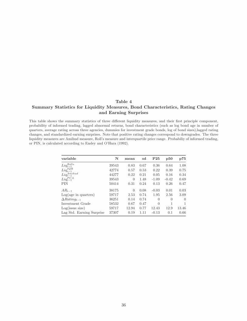
Table 4Summary Statistics for Liquidity Measures, Bond Characteristics, Rating Changes

and Earning Surprises

This table shows the summary statistics of three different liquidity measures, and their first principle component,probability of informed trading, lagged abnormal returns, bond characteristics (such as log bond age in number ofquarters, average rating across three agencies, dummies for investment grade bonds, log of bond sizes),lagged ratingchanges, and standardized earning surprises. Note that positive rating changes correspond to downgrades. The threeliquidity measures are Amihud measure, Roll’s measure and interquartile price range. Probabiliy of informed trading,or PIN, is calculated according to Easley and O’Hara (1992).

variable N mean sd P25 p50 p75

LiqRollst−1 39543 0.83 0.67 0.36 0.64 1.08

LiqIQRt−1 42774 0.57 0.53 0.22 0.39 0.75

LiqAmihudt−1 44277 0.22 0.21 0.05 0.16 0.34

LiqPCAt−1 39543 0 1.48 -1.09 -0.42 0.69

PIN 50414 0.31 0.24 0.13 0.26 0.47

ARt−1 38175 0 0.08 -0.03 0.01 0.03Log(age in quarters) 59717 2.53 0.74 1.95 2.56 3.09∆Ratingt−1 36251 0.14 0.74 0 0 0Investment Grade 58532 0.67 0.47 0 1 1Log(issue size) 59717 12.94 0.77 12.43 12.9 13.46Lag Std. Earning Surprise 37307 0.19 1.11 -0.13 0.1 0.66

36

Table 5Cross-sectional Determinant of Herding

This table shows results from quarterly Fama-MacBeth regressions of institutional fund herding (Buy and Sell) onon bond characteristics, events, liquidity measures and probability of informed trading. Bond characteristics includelogged bond age, lagged rating changes, average rating across three agencies, dummies for investment grade bonds,log of the par amount at issuance. Events related variables include the lagged rating changes (positive rating changescorrespond to downgrades) and standardized earning surprises. Standardized earning surprises are calculated bydividing earning surprises by the time -series standard deviation of surprises. Lagged abnormal return is also used asa control variable to account for momentum effect. Finally, the first principle component of the three different liquiditymeasures is used as a measure of secondary market liquidity. The three liquidity measures are Amihud measure, Roll’smeasure and interquartile price range. Probabiliy of informed trading, or PIN, is calculated according to Easley andO’Hara (1992).

Regressor Buy Sell

(1) (2) (3) (4) (1) (2) (3) (4)ARt−1 -0.022 -0.030 -0.051 -0.059 -0.037 -0.031 0.037 -0.020

(-1.51) (-1.51) (-1.43) (-1.28) (-1.23) (-1.02) (0.88) (-0.46)Log(age) -0.006** -0.006** -0.004 -0.003 0.008** 0.003 0.006 0.006

(-2.25) (-2.50) (-1.70) (-0.99) (2.57) (0.80) (1.43) (1.42)∆Ratingt−1 -0.011*** -0.011*** -0.009** -0.008 0.011** 0.008 0.008 0.012

(-3.56) (-3.17) (-2.38) (-1.66) (2.83) (1.65) (1.47) (1.38)Current Rating -0.000 0.000 0.001 0.002** 0.004*** 0.003*** 0.003*** 0.003***

(-0.56) (0.21) (1.27) (2.51) (5.52) (5.21) (4.15) (3.14)Investment Grade -0.013* -0.011 -0.007 -0.005 -0.029*** -0.031*** -0.034*** -0.031*

(-1.79) (-1.41) (-0.77) (-0.56) (-4.87) (-4.29) (-3.63) (-1.89)Log(issuesize) -0.012*** -0.012*** -0.011*** -0.007** -0.001 0.002 0.006 0.005

(-6.10) (-5.87) (-3.61) (-2.22) (-0.33) (0.50) (1.24) (1.12)LiqPCA

t−1 0.001 0.002 0.002 0.001 0.001 0.001(0.79) (0.98) (1.01) (0.98) (0.87) (1.15)

Lag Std. Earning Surprise 0.000 0.000 -0.004*** -0.005**(0.33) (0.31) (-2.99) (-2.56)

PIN 0.012 0.022**(1.35) (2.18)

cons 0.245*** 0.246*** 0.218*** 0.154*** 0.029 0.005 -0.048 -0.046(9.37) (9.28) (5.48) (3.71) (0.79) (0.11) (-0.89) (-0.91)

r2 0.030 0.033 0.040 0.047 0.071 0.076 0.091 0.110N 17102 14892 10056 6237 13481 11352 7663 4714

37

Table 6Herding and Transparency

The shows results from Newey-West regression for the impact of transparency on buy and sell herding. Bonds thatwere in each stage of the transparency regime and bonds that were never required to report to TRACE are all included.Stage 1 bonds are those that were included in TRACE reporting since the beginning of our sample (2003Q4). Stage2 & 3 bonds are those that were added to TRACE dissemination list on Oct. 2004 and Feb. 2005. We combine thetwo events as they are very close to each other. Post stage 2 & 3 is the time dummy that takes the value of 1 if thequarter is after Q1- 2005, 0 if the quarter is before Q4-2004 and missing if the quarter is between or on Q4-2004 andQ1 2005. Other control variables are similar to those in Table 5. Liquidity measures are not included as they arenot available for bond-quarters when trades are not reported to TRACE. We use Newey-West method, instead ofthe Fama-Macbeth method, to control for autocorrelation since Fama-Macbeth can not be used when there is a timedummy.

Regressors Buy SellCoef./T Coef./T

Stage 1 added bonds 0.001 -0.005(0.30) (-0.93)

Stage 2 & 3 bonds -0.015* 0.001(-1.77) (0.06)

Post Stage 2 & 3 0.001 -0.003(0.27) (-0.39)

Stage 2 & 3 bonds*Post Stage 2 & 3 0.020** -0.001(2.53) (-0.13)

ARt−1 0.017 -0.016(0.99) (-0.79)

Log(age in quarters) -0.006** 0.011***(-2.14) (3.34)

Log(issue size) -0.009*** 0.002(-4.18) (0.84)

∆Ratingt−1 -0.008*** 0.012***(-2.91) (3.52)

Lag Std. Earning Surprise 0.000 -0.006***(0.26) (-4.30)

Current Rating -0.000 0.003***(-0.11) (4.62)

Investment Grade -0.021*** -0.031***(-4.11) (-5.15)

cons 0.209*** -0.008(6.85) (-0.20)

r2 0.014 0.054N 10313 7969

38

Table 7Evidence of Imitational Trading

This table reports results from tests similar to those in Table 3 of Sias (2004). For each bond and quarter, we calculatethe fraction of institutional traders that increased their holdings in the security. All data are standardized(i.e, rescaledto zero mean, unit variance) each quarter. We then estimate cross-sectional regressions of institutional demand onlag institutional demand. The first column reports the time-series average of all quarterly regression coefficients.The second and third column report the portion of the correlation that results from institutional investors followingtheir own lag trades and the portion that results from institutions following the previous trades of other institutions(herding). The symbols *, ** and *** indicate significance at the 5%, 1% and .1% levels, respectively.

Partitioned Slope Coefficients β in ∆k,t = β ∗∆k,t−1 + ǫk,t

Average coefficients (β) Institutions follow their own trades Institutions follow others’ tradeSecurities with >= 5 traders

0.251 0.008 0.238(16.90)*** (1.90)* (17.95)***

Securities with >= 10 traders0.282 0.005 0.273

(16.57)*** (1.55) (17.376)***

39

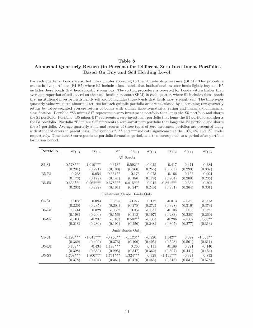
Table 8Abnormal Quarterly Return (in Percent) for Different Zero Investment Portfolios

Based On Buy and Sell Herding Level

For each quarter t, bonds are sorted into quintiles according to their buy-herding measure (BHM). This procedureresults in five portfolios (B1-B5) where B1 includes those bonds that institutional investor herds lightly buy and B5includes those bonds that herds mostly strong buy. The sorting procedure is repeated for bonds with a higher thanaverage proportion of sells based on their sell-herding measure(SHM) in each quarter, where S1 includes those bondsthat institutional investor herds lightly sell and S5 includes those bonds that herds most strongly sell. The time-seriesquarterly value-weighted abnormal returns for each quintile portfolio are are calculated by subtracting raw quarterlyreturn by value-weighted average return of bonds with similar time-to-maturity, rating and financial/nonfinancialclassification. Portfolio “S5 minus S1” represents a zero-investment portfolio that longs the S5 portfolio and shortsthe S1 portfolio. Portfolio “B5 minus B1” represents a zero-investment portfolio that longs the B5 portfolio and shortsthe B1 portfolio. Portfolio “B5 minus S5” represents a zero-investment portfolio that longs the B5 portfolio and shortsthe S5 portfolio. Average quarterly abnormal returns of three types of zero-invetment porfolios are presented alongwith standard errors in parentheses. The symbols *, ** and *** indicate significance at the 10%, 5% and 1% levels,respectively. Time label t corresponds to portfolio formation period, and t+n corresponds to n period after portfolioformation period.

Portfolio art−2 art−1 ar art+1 art+2 art+3 art+4 art+5

All Bonds

S5-S1 -0.578*** -1.019*** -0.373* -0.592** -0.025 0.417 0.471 -0.384(0.201) (0.221) (0.198) (0.260) (0.255) (0.303) (0.293) (0.337)

B5-B1 0.268 -0.054 0.334** 0.173 0.073 -0.166 0.155 0.004(0.173) (0.178) (0.141) (0.186) (0.179) (0.204) (0.208) (0.235)

B5-S5 0.636*** 0.962*** 0.678*** 0.815*** 0.042 -0.821*** -0.355 0.302(0.203) (0.222) (0.191) (0.247) (0.240) (0.291) (0.264) (0.301)

Investment Grade Bonds Only

S5-S1 0.168 0.083 0.325 -0.277 0.172 -0.013 -0.260 -0.373(0.220) (0.235) (0.204) (0.278) (0.272) (0.328) (0.316) (0.373)

B5-B1 0.244 0.028 -0.082 0.054 -0.031 -0.105 0.108 0.321(0.198) (0.206) (0.156) (0.213) (0.197) (0.233) (0.228) (0.260)

B5-S5 -0.100 -0.237 -0.163 0.502** -0.063 -0.286 -0.007 0.666**(0.218) (0.230) (0.191) (0.256) (0.248) (0.305) (0.277) (0.313)

Junk Bonds Only

S5-S1 -1.190*** -1.641*** -0.756** -1.123** -0.220 1.142** 0.892 -1.333**(0.369) (0.402) (0.376) (0.496) (0.495) (0.528) (0.561) (0.611)

B5-B1 0.708** -0.434 1.198*** 0.260 0.111 -0.188 0.221 -0.140(0.328) (0.332) (0.295) (0.347) (0.362) (0.397) (0.441) (0.454)

B5-S5 1.708*** 1.800*** 1.761*** 1.324*** 0.329 -1.411*** -0.327 0.852(0.378) (0.404) (0.361) (0.476) (0.465) (0.516) (0.531) (0.578)

40

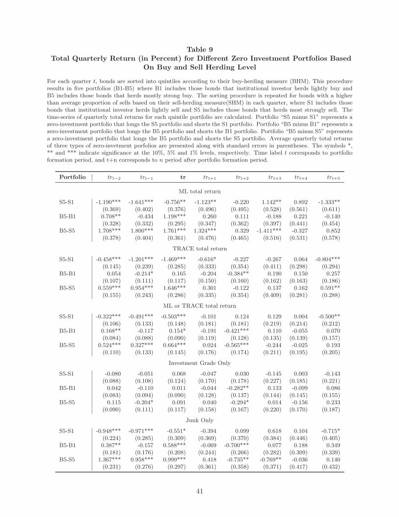
Table 9Total Quarterly Return (in Percent) for Different Zero Investment Portfolios Based

On Buy and Sell Herding Level

For each quarter t, bonds are sorted into quintiles according to their buy-herding measure (BHM). This procedureresults in five portfolios (B1-B5) where B1 includes those bonds that institutional investor herds lightly buy andB5 includes those bonds that herds mostly strong buy. The sorting procedure is repeated for bonds with a higherthan average proportion of sells based on their sell-herding measure(SHM) in each quarter, where S1 includes thosebonds that institutional investor herds lightly sell and S5 includes those bonds that herds most strongly sell. Thetime-series of quarterly total returns for each quintile portfolio are calculated. Portfolio “S5 minus S1” represents azero-investment portfolio that longs the S5 portfolio and shorts the S1 portfolio. Portfolio “B5 minus B1” represents azero-investment portfolio that longs the B5 portfolio and shorts the B1 portfolio. Portfolio “B5 minus S5” representsa zero-investment portfolio that longs the B5 portfolio and shorts the S5 portfolio. Average quarterly total returnsof three types of zero-invetment porfolios are presented along with standard errors in parentheses. The symbols *,** and *** indicate significance at the 10%, 5% and 1% levels, respectively. Time label t corresponds to portfolioformation period, and t+n corresponds to n period after portfolio formation period.

Portfolio trt−2 trt−1 tr trt+1 trt+2 trt+3 trt+4 trt+5

ML total return

S5-S1 -1.190*** -1.641*** -0.756** -1.123** -0.220 1.142** 0.892 -1.333**(0.369) (0.402) (0.376) (0.496) (0.495) (0.528) (0.561) (0.611)

B5-B1 0.708** -0.434 1.198*** 0.260 0.111 -0.188 0.221 -0.140(0.328) (0.332) (0.295) (0.347) (0.362) (0.397) (0.441) (0.454)

B5-S5 1.708*** 1.800*** 1.761*** 1.324*** 0.329 -1.411*** -0.327 0.852(0.378) (0.404) (0.361) (0.476) (0.465) (0.516) (0.531) (0.578)

TRACE total return

S5-S1 -0.458*** -1.201*** -1.469*** -0.616* -0.227 -0.267 0.064 -0.804***(0.145) (0.239) (0.285) (0.333) (0.354) (0.411) (0.298) (0.294)

B5-B1 0.054 -0.214* 0.165 -0.204 -0.384** 0.190 0.150 0.257(0.107) (0.111) (0.117) (0.150) (0.160) (0.162) (0.163) (0.186)

B5-S5 0.559*** 0.954*** 1.646*** 0.301 -0.122 0.137 0.162 0.591**(0.155) (0.243) (0.286) (0.335) (0.354) (0.409) (0.281) (0.288)

ML or TRACE total return

S5-S1 -0.322*** -0.491*** -0.503*** -0.101 0.124 0.129 0.004 -0.500**(0.106) (0.133) (0.148) (0.181) (0.181) (0.219) (0.214) (0.212)

B5-B1 0.168** -0.117 0.154* -0.191 -0.421*** 0.110 -0.055 0.070(0.084) (0.088) (0.090) (0.119) (0.128) (0.135) (0.139) (0.157)

B5-S5 0.524*** 0.327*** 0.664*** 0.024 -0.565*** -0.244 -0.025 0.193(0.110) (0.133) (0.145) (0.176) (0.174) (0.211) (0.195) (0.205)

Investment Grade Only

S5-S1 -0.080 -0.051 0.068 -0.047 0.030 -0.145 0.003 -0.143(0.088) (0.108) (0.124) (0.170) (0.178) (0.227) (0.185) (0.221)

B5-B1 0.042 -0.110 0.011 -0.044 -0.282** 0.133 -0.099 0.086(0.083) (0.094) (0.090) (0.128) (0.137) (0.144) (0.145) (0.155)

B5-S5 0.115 -0.204* 0.091 0.040 -0.294* 0.014 -0.156 0.233(0.090) (0.111) (0.117) (0.158) (0.167) (0.220) (0.170) (0.187)

Junk Only

S5-S1 -0.948*** -0.971*** -0.551* -0.394 0.099 0.618 0.104 -0.715*(0.224) (0.285) (0.309) (0.369) (0.370) (0.384) (0.446) (0.405)

B5-B1 0.387** -0.157 0.588*** -0.069 -0.700*** 0.077 0.188 0.349(0.181) (0.176) (0.208) (0.244) (0.266) (0.282) (0.309) (0.339)

B5-S5 1.367*** 0.958*** 0.999*** 0.418 -0.735** -0.769** -0.036 0.140(0.231) (0.276) (0.297) (0.361) (0.358) (0.371) (0.417) (0.432)

41

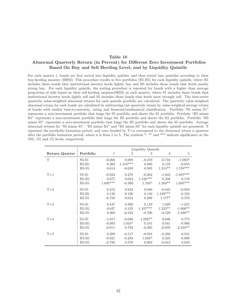
Table 10Abnormal Quarterly Return (in Percent) for Different Zero Investment Portfolios

Based On Buy and Sell Herding Level, and by Liquidity Quintile

For each quarter t, bonds are first sorted into liquidity quitiles, and then sorted into quintiles according to theirbuy-herding measure (BHM). This procedure results in five portfolios (B1-B5) for each liquidity quintile, where B1includes those bonds that institutional investor herds lightly buy and B5 includes those bonds that herds mostlystrong buy. For each liquidity quintile, the sorting procedure is repeated for bonds with a higher than averageproportion of sells based on their sell-herding measure(SHM) in each quarter, where S1 includes those bonds thatinstitutional investor herds lightly sell and S5 includes those bonds that herds most strongly sell. The time-seriesquarterly value-weighted abnormal returns for each quintile portfolio are calculated. The quarterly value-weightedabnormal return for each bonds are calculated by subtracting raw quarterly return by value-weighted average returnof bonds with similar time-to-maturity, rating and financial/nonfinancial classification. Portfolio “S5 minus S1”represents a zero-investment portfolio that longs the S5 portfolio and shorts the S1 portfolio. Portfolio “B5 minusB1” represents a zero-investment portfolio that longs the B5 portfolio and shorts the B1 portfolio. Portfolio “B5minus S5” represents a zero-investment portfolio that longs the B5 portfolio and shorts the S5 portfolio. Averageabnormal returns for “S5 minus S1”, “B5 minus B1” and “B5 minus S5” for each liquidity quintile are presented. Trepresent the portforlio formation period, and rows headed by T+n correspond to the abnormal return n quartersafter the portfolio formation period, where n is from 1 to 5. The symbols *, ** and *** indicate significance at the10%, 5% and 1% levels, respectively.

Liquidity QuintileReturn Quarter Portfolio 1 2 3 4 5

T S5-S1 -0.266 0.088 -0.219 -0.716 -1.083*B5-B1 0.269 1.418*** 0.080 0.135 -0.055B5-S5 0.614 -0.059 0.595 1.314** 1.576***

T+1 S5-S1 -0.924 0.278 -0.262 -1.043 -1.887***B5-B1 0.677 0.024 1.156*** 0.438 0.178B5-S5 1.695*** -0.390 1.194* 1.350** 1.695***

T+2 S5-S1 0.472 0.622 0.046 -0.845 -0.910B5-B1 0.138 0.196 0.146 1.439*** -0.162B5-S5 -0.750 0.014 0.289 1.177* 0.576

T+3 S5-S1 0.447 0.360 0.143 1.029 -1.231B5-B1 0.837 0.135 -1.457*** 1.225** -1.600**B5-S5 0.300 -0.333 -0.706 -0.529 -1.830**

T+4 S5-S1 -1.617 -0.036 1.958** 0.646 0.775B5-B1 -0.093 1.043* 0.161 0.941 -0.906B5-S5 -0.011 0.793 -0.305 -0.076 -2.103**

T+5 S5-S1 0.209 -0.517 -0.916 -0.280 0.531B5-B1 -0.921 -0.283 1.038* 0.325 -0.008B5-S5 -0.780 0.570 0.963 -0.012 0.633

42