Embed Size (px)
Citation preview
Understanding Frequency Response of a Flexural Complaint Stage for use in
Oscillatory Orthogonal Cutting
by
Raul Barraza
Submitted to theDepartment of Mechanical Engineering
in Partial Fulfillment of the Requirements for the Degree of
ARCHNESMASSACHUSETTS INSTITUTE
OF TECHNOLOLGy
JUN 2 4 2015
LIBRARIES
Bachelor of Science in Mechanical Engineering
at the
Massachusetts Institute of Technology
June 2015
2015 Massachusetts Institute of Technology. All rights reserved.
Signature redactedSignature of Author:
SiCertified by:
C' rtment of Mechanical Engineering2' May 26,2015
gnature redactedMartin L. Culpepper
Signature redactedProfessor of Mechanical Engineering
Thesis Supervisor
Accepted by:Anette Hosoi
Professor of Mechanical EngineeringUndergraduate Officer
1

2
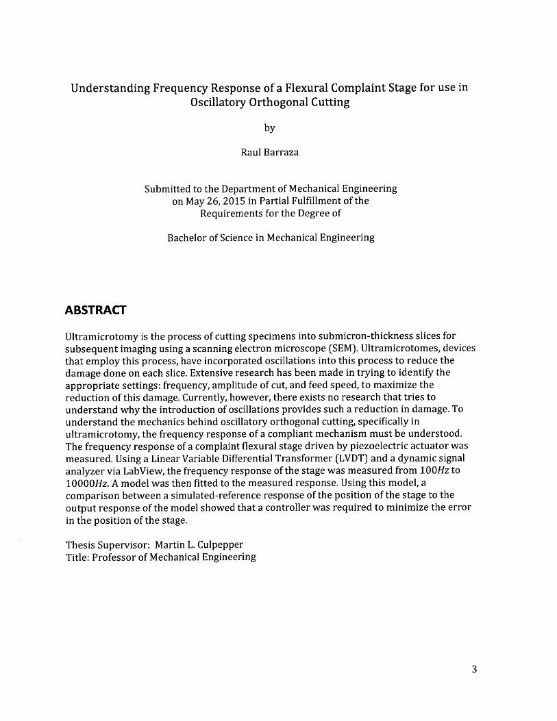
Understanding Frequency Response of a Flexural Complaint Stage for use inOscillatory Orthogonal Cutting
by
Raul Barraza
Submitted to the Department of Mechanical Engineeringon May 26, 2015 in Partial Fulfillment of the
Requirements for the Degree of
Bachelor of Science in Mechanical Engineering
ABSTRACT
Ultramicrotomy is the process of cutting specimens into submicron-thickness slices forsubsequent imaging using a scanning electron microscope (SEM). Ultramicrotomes, devicesthat employ this process, have incorporated oscillations into this process to reduce thedamage done on each slice. Extensive research has been made in trying to identify theappropriate settings: frequency, amplitude of cut, and feed speed, to maximize thereduction of this damage. Currently, however, there exists no research that tries tounderstand why the introduction of oscillations provides such a reduction in damage. Tounderstand the mechanics behind oscillatory orthogonal cutting, specifically inultramicrotomy, the frequency response of a compliant mechanism must be understood.The frequency response of a complaint flexural stage driven by piezoelectric actuator wasmeasured. Using a Linear Variable Differential Transformer (LVDT) and a dynamic signalanalyzer via LabView, the frequency response of the stage was measured from 100Hz to10000Hz. A model was then fitted to the measured response. Using this model, acomparison between a simulated-reference response of the position of the stage to theoutput response of the model showed that a controller was required to minimize the errorin the position of the stage.
Thesis Supervisor: Martin L. CulpepperTitle: Professor of Mechanical Engineering
3

AcknowledgementI would like to thank Professor. David Trumper for providing me access to his lab and
allowing access to all the equipment in the lab. I would like to thank Tyler Hamer for
providing me with his dynamic signal analyzer, and for his help along this whole process. I
would like to thank Mark Belanger at the Edgerton Student Shop for aiding me during use
of the shop. Finally, I would like to thank Aaron Ramirez and Martin Culpepper for their
guidance in this project.
4

Table of Contents
ABSTRACT ......................................................................................................................................................... 3
ACKNOW LEDGEMENT.........................................................................................................................................4
LIST OF FIGURES........................................................................................................................................7
CHAPTER 1: INTRODUCTION.......................................................................................................................8
1.1 IN TR O D U C TIO N ................................................................................................................................................. 8
1.2 B A C K G R O U N D ................................................................................................................................................... 81.2.1 INTRODUCTION To FINAL PRODUCT 8
1.2.2 CURRENT TECHNOLOGY & SPECIFIC MOTIVATION 10
1.2.3 LARGER PICTURE 12
1.3 P R IO R A R T ...................................................................................................................................................... 12
CHAPTER 2: FUNDAMENTALS OF OSCILLATORY OBLIQUE CUTTING ........................... 14
2.1 ORTHOGONAL CUTTING .............................................................................................................................. 14
2.2 MERCHAN T'S MODEL ................................................................................................................................... 142.2.1 SHEAR 162.2.2 FORCES & STRESSES 18
2.2.3 VELOCITY RELATIONS 19
2.2.4 STRAIN RATE 20
2.2.5 ENERGY APPROACH 20
2.3 OBLIQUE CUTTING........................................................................................................................................ 212.3.1 CUTTING FORCES ......................................................................................................................................... 222.3.2 RECIPROCATING BLADES............................................................................................................................. 24
CHAPTER 3: COMPLIANT STRUCTURES .......................................................................................... 25
3.1 COMPLIANT FLEXURAL SYSTEMS.............................................................................................................. 253.2 PIEZOELECTRIC ACTUATORS ..................................................................................................................... 27
CHAPTER 4: ASSESSMENT OF DESIGN AND THEORY .............................................................. 30
4.1 VIBRATING FLEXURAL STAGE DESIGN................................................................................................. 30
4.1.1 DESIGN SPECIFICATIONS 30
4.1.2 LINEAR STAGE DESIGN 30
4.1.3 CHARACTERIZATION OF ACTUATOR PERFORMANCE 32
4.1.4 DYNAMIC DESIGN 334.1.5: FLEXURAL STAGE DESIGN 35
4.1.6: ACTUATOR CONNECTION 35
4.2 DYNAMIC BEHAVIOR ....................................................................................................................................... 37
CHAPTER 5: VALIDATION OF DESIGN .............................................................................................. 40
5.1 INSTRUMENTATION AND SETUP.................................................................................................................. 40
CHAPTER 6: RESULTS & DISCUSSION............................................................................................... 43
6.1: EXPERIMENTAL RESULTS .......................................................................................................................... 43
5

CHAPTER 7: CONCLUSION........................................... ..................................................................... 48
7 .1 FUTURE W ORK ................................................................................................................................................ 4 87.1.1: CHARACTERIZATION OF FLEXURAL STAGE DESIGN 48
7.1.2: IMPLEMENTATION OF A CONTROLLER 48
BIBLIOGRAPHY ..................................................................... ................................................................. 49
6
List of FiguresFigu re 1: D raw ing of th e D evice......................................................................................................................... 9Figu re 2 : Im age of Fin al D evice .......................................................................................................................... 9Figure 3:Measured Frequency Response with Fitted Model......................................................... 10Figure 4: Process of U ltram icrotom y........................................................................................................ 11Figure 5: Three commercial ultramicrotomes sold in the market.............................................. 11Figure 6: Figure of merchant's model for orthogonal cutting with primary shear plane, tool, and
c h ip l4 ............................................................................................................................................................... 1 5Figure 7: Graphical Representation of the three primary shear zones experienced in metal
cutting. A) Merchant's model for the primary shear plane. B) Pie-shaped shear zone seenwhen cutting soft and prestrained materials. C) Undefined shear zone seen in metal cutting
when tool has radius that significantly large relative to depth of cut|4j................................ 15
Figure 8: Pictorial Representation of the geometric relationship between shear angle and the
cutting ratio. a is the rake angle, the angle from the tool face to the normal from the
w o rk p iece l4 1................................................................................................................................................... 1 7Figure 9: Pictorial representation of the shear strain that occurs in orthogonal cuttingl4l........... 17
Figure 10: M erchant's Com posite Circle[4] ........................................................................................... 18Figure 11: Pictorial Representation of the velocity diagram41......................................................... 19
Figure 12: Three situation of oblique cutting from which the slice-push ratio exists5 .......... 21
Figure 13: Pictorial representation of the displacements seen in an orthogonal blademoving parallel and normal to the cutting edge of the blade[5]. ...................................... 22
Figure 14: 1) Pictorial Representation of the four components that comprise a complaintstructure. 2) Cantilevered Beam used to model flexure deflection[7]............................ 25
Figure 16: Different Piezoelectric actuators available in the market. 1) Stacked Piezoelectricactuator. 2) Plate Piezoelectric Actuator. 3) Bender Piezoelectric Actuator[7].......... 28
Figure 17: Diagram of Stacked Piezoelectric Actuator Geometry[7]......................................... 29Figure 19: A ctuator Perform ance................................................................................................................... 32Figure 21: Final Design of Stage Design Values presented are valued measured post-
fa b rica tio n ....................................................................................................................................................... 3 5Figure 22: Final assembled actuator installed into stage. .............................................................. 37Figure 24: Expected frequency response of system........................................................................... 39Figure 25: Assem bled Calibration Setup.............................................................................................. 40Figure 26: Comparison of Output Voltage to Core Displacement. ............................................... 41Figure 27: Final Test Setup of Stage with LVDT sensor and signal conditioner.................... 42Figure 28:Comparison of Expected Response to Measured Response ..................................... 43Figure 29: Comparison Fitted Model to Measured Response ...................................................... 45Figure 30: Simulated Input compared against output response of system ............................ 46Figure 31: Nyquist plot of fitted m odel.................................................................................................. 46
7
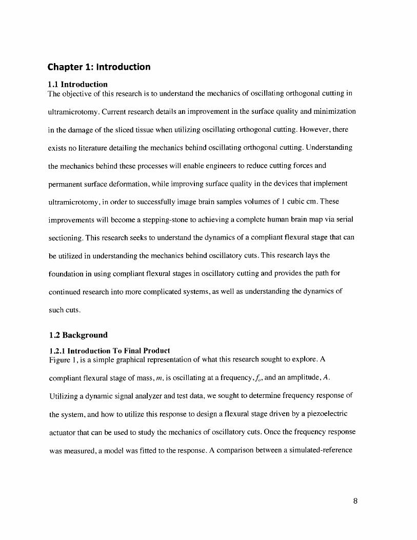
Chapter 1: Introduction
1.1 IntroductionThe objective of this research is to understand the mechanics of oscillating orthogonal cutting in
ultramicrotomy. Current research details an improvement in the surface quality and minimization
in the damage of the sliced tissue when utilizing oscillating orthogonal cutting. However, there
exists no literature detailing the mechanics behind oscillating orthogonal cutting. Understanding
the mechanics behind these processes will enable engineers to reduce cutting forces and
permanent surface deformation, while improving surface quality in the devices that implement
ultramicrotomy, in order to successfully image brain samples volumes of 1 cubic cm. These
improvements will become a stepping-stone to achieving a complete human brain map via serial
sectioning. This research seeks to understand the dynamics of a compliant flexural stage that can
be utilized in understanding the mechanics behind oscillatory cuts. This research lays the
foundation in using compliant flexural stages in oscillatory cutting and provides the path for
continued research into more complicated systems, as well as understanding the dynamics of
such cuts.
1.2 Background
1.2.1 Introduction To Final ProductFigure 1, is a simple graphical representation of what this research sought to explore. A
compliant flexural stage of mass, m, is oscillating at a frequency,fo, and an amplitude, A.
Utilizing a dynamic signal analyzer and test data, we sought to determine frequency response of
the system, and how to utilize this response to design a flexural stage driven by a piezoelectric
actuator that can be used to study the mechanics of oscillatory cuts. Once the frequency response
was measured, a model was fitted to the response. A comparison between a simulated-reference
8

response for the position of the stage and the output response of the model showed that a
controller is required in reducing the error of the system.
Figure 1: Drawing of the Device
IFigure 2: Image of Final Device
9
100
10~ 2310 10
500
0--Measured Response
CU
-500 2 310 10
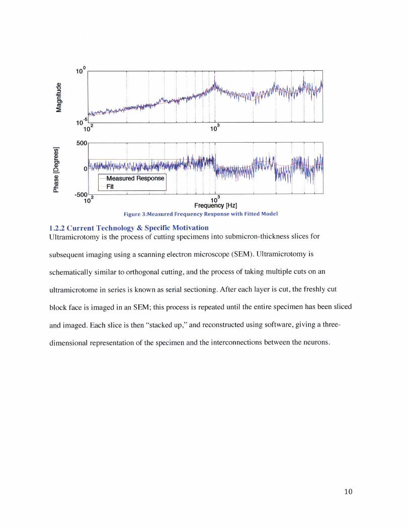
Frequency [Hz]Figure 3:Measured Frequency Response with Fitted Model
1.2.2 Current Technology & Specific MotivationUltramicrotomy is the process of cutting specimens into submicron-thickness slices for
subsequent imaging using a scanning electron microscope (SEM). Ultramicrotomy is
schematically similar to orthogonal cutting, and the process of taking multiple cuts on an
ultramicrotome in series is known as serial sectioning. After each layer is cut, the freshly cut
block face is imaged in an SEM; this process is repeated until the entire specimen has been sliced
and imaged. Each slice is then "stacked up," and reconstructed using software, giving a three-
dimensional representation of the specimen and the interconnections between the neurons.
10
L
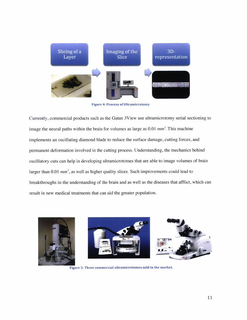
Figure 4: Process of Ultramicrotomy
Currently, commercial products such as the Gatan 3View use ultramicrotomy serial sectioning to
image the neural paths within the brain for volumes as large as 0.01 mm'. This machine
implements an oscillating diamond blade to reduce the surface damage, cutting forces, and
permanent deformation involved in the cutting process. Understanding, the mechanics behind
oscillatory cuts can help in developing ultramicrotomes that are able to image volumes of brain
larger than 0.01 mm', as well as higher quality slices. Such improvements could lead to
breakthroughs in the understanding of the brain and as well as the diseases that afflict, which can
result in new medical treatments that can aid the greater population.
Figure 5: Three commercial ultramicrotomes sold in the market.
11

1.2.3 Larger PictureAlthough the main motivation for understanding the mechanics behind such cutting process
stems from trying to improve existing ultramicrotomes, this research has implication beyond this
area. Oscillatory cutting process is not only used in slicing of brain samples in ultramicrotomy,
but as well as in surgical tools in the medical field, and, metal cutting processes involved in
several industries. Considering the medical field alone, various surgical tools, such as surgical
bone saws, employ oscillatory cuts when being operated. Understanding the mechanics these
cuts could lead to surgical tools that provide minimal damage to patient tissue during surgery,
thus minimizing patient's recovery time, and saving millions of dollars in care and treatment.
Metal cutting processes are a large component in several manufacturing industries, including
aeronautical, automotive, and electrical. With each of these industries outputting large volumes
of products a day, small improvements in the metal cutting processes involved could lead to
millions of dollars saved in energy consumption and material conserved. This research aims to
give designers a new tool that aids in the design of devices that employ oscillatory cuts in order
improve existing practices.
1.3 Prior ArtVery little work has been done in understanding the mechanics behind oscillatory cutting in
ultramicrotomy. Most of the research involving such oscillatory cuts incorporates oscillations
into ultramicrotomy to reduce the cutting artefacts in each slice: compression, crevasses and
chatter. Compression is the shortening of the slice's length parallel to the cutting direction,
resulting in an increase in the thickness of the slice with minimal change across the length
perpendicular to the cutting direction. Crevasses are a system of fractures penetrating the slice
from one side. Chatter is the periodic variation of the thickness of the slice along the cutting
12

direction[I]. These cutting artefacts create inconsistencies in the tissue slices that diminish the
accuracy provided by the 3D representation of the scanned tissue samples. According to the
research done by Daniel Studer, Ashraf Al-Amoudi, and Kasim Sader, incorporating
oscillations varying from 2kHz-4OkHz with a stroke of 20nm - 400nm minimizes any chatter and
crevassesi I] seen in the slice, and reduces compression by 15%[2]. In addition, research headed
by Hongyan Gu characterized the complete removal of chatter when cutting at a frequency
higher than 25 kHz and a cutting speed of greater than 0.2 mm/s (cutting speed is the velocity at
which the sample was feed into the oscillating blade)[3]. In most biological practices, the
understanding of the mechanics behind oscillatory cuts is not critical as long as the
improvements are seen during the process of ultramicrotomy. This could explain the limited
amount of research in trying to understand oscillatory cutting processes.
13
Chapter 2: Fundamentals of Oscillatory Oblique Cutting
2.1 Orthogonal CuttingSimple orthogonal cutting is a metal cutting process representative of the cutting mechanics in
many machining operations, such as turning, planing, and facing. In orthogonal cutting, as metal
approaches the edge of the tool, it deforms by shear. As the material shears, it plastically
deforms, creating chips that flow up the orthogonal plane, the face of the tool 14]. Given the good
approximation of orthogonal cutting for the major cutting edges in many machining operations,
several models have been created in order to understand the mechanics behind this cutting
process. Each of these models is an idealized case for the cutting process in orthogonal cutting,
and each holds its own limitations.
2.2 Merchant's ModelMerchant's model is an idealized model of the orthogonal cutting that represents the formation of
chips through the concentration of a shearing process across the primary shearing plane. In this
model, the material is considered to be homogenous via the following assumptions[4]:
1. The tool is perfectly sharp and there is no contact along the clearance face.
2. The shear surface is a plane extending upward from the cutting edge by and angle, 4.
3. The cutting edge is a straight line extending orthogonal to the direction of motion and
generates a plane surface as the work moves past it.
4. The chip does not flow to either side (i.e. plane strain).
5. The depth of cut is constant.
6. The width of the tool is greater than that of the workpiece.
7. The work moves relative to the tool with uniform velocity.
8. A continuous chip is produced with no built-up edge.
9. The shear and normal stresses along shear plane and tool are uniform.
14

Chip ""'*width
ChiC
Tool
secwndaryAhear
.zone
Primary Shearzone
Figure 6: Figure of merchant's model for orthogonal cutting with primary shear plane, tool, and chipl4l
The model, however, fails when the workpiece is soft and not prestrain hardened before
cutting, or when the radius of the tool is of significant size relative to the undeformed chip
thickness. In these two cases, the shear plane becomes either a pie-shaped zone or an
undefined shear zone[4].
(a) (b) (c)
Figure 7: Graphical Representation of the three primary shear zones experienced in metal cutting. A) Merchant's modelfor the primary shear plane. B) Pie-shaped shear zone seen when cutting soft and prestrained materials. C) Undefinedshear zone seen in metal cutting when tool has radius that significantly large relative to depth of cut[4I.
15

2.2.1 ShearIn Merchant's model, the primary shear plane is defined by the shear angle, q, which is the angle
from the straight line extending from the cutting edge. This angle can be defined using the
cutting ratio, r, the ratio of the depth of cut, t, to the chip thickness, t. Given that there is no
change in the density of the material when cut, the volume of the undeformed chip equals the
volume of the chip. Thus, the cutting ratio can be defined as follows:
__ tr= =
This is assuming that the ratio of the width of cut and the depth of cut, t, are greater than or equal
to five. By looking at the geometric relationships between the workpiece, the chip, and the
primary shear plane, the relationship between the cutting ratio and the shear angle is defined as
follows:
r = ABsink) [2]ABCOS((P-a)
Thus, the shear angle can be defined as follows:
tan(p = rsa [3]
16
Chip
B CTool
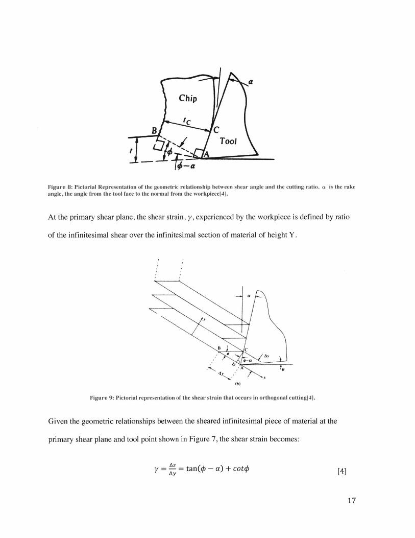
Figure 8: Pictorial Representation of the geometric relationship between shear angle and the cutting ratio. a is the rakeangle, the angle from the tool face to the normal from the workpiece[4].
At the primary shear plane, the shear strain, y, experienced by the workpiece is defined by ratio
of the infinitesimal shear over the infinitesimal section of material of height Y.
Figure 9: Pictorial representation of the shear strain that occurs in orthogonal cuttingl4j.
Given the geometric relationships between the sheared infinitesimal piece of material at the
primary shear plane and tool point shown in Figure 7, the shear strain becomes:
y = = tan(k - a) + cot [4A~Y[4
17

Where the a is the rake angle, # is the shear angle, and ly is the thickness of the shear zone.
2.2.2 Forces & StressesTwo forces are present during orthogonal cutting: a force, R, at the interface between the tool
face and the chip, and a force, R', at the interface between the workpiece and the chip along the
shear plane. These forces can be broken down into a set of three components acting along the x
and y directions (FP and FQ, respectively), as well as normal and perpendicular to the two
interfaces of the chip (Fs and Fc respectively). Translating these forces to the point of the tool,
the composite cutting force circle is created where the R is the diameter of the circle. Thus, the
shear and friction forces, and the coefficient of friction at the two interfaces of the chip can be
defined as functions of the geometric relationships of the this diagram, and Fp and FQ.
Figure 10: Merchant's Composite Circle[41.
Given this, the mean shear and normal stresses on the shear plane can be defined as functions of
the same geometric values and the forces from the composite cutting circle in Figure 8. Thus, the
mean shear stress and the normal stress can be defined as follows, where A, is the area of the
shear plane:
18
As = bt
Fs _ (FpcosO-Fsin)sinp [6]As bt
_ Ls = (FpCOSCP+FQSin )sin(P [7As bt
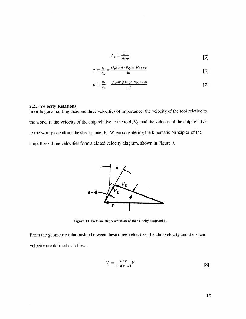
2.2.3 Velocity RelationsIn orthogonal cutting there are three velocities of importance: the velocity of the tool relative to
the work, V, the velocity of the chip relative to the tool, Vc, and the velocity of the chip relative
to the workpiece along the shear plane, Vs. When considering the kinematic principles of the
chip, these three velocities form a closed velocity diagram, shown in Figure 9.
Figure 11: Pictorial Representation of the velocity diagram|4I.
From the geometric relationship between these three velocities, the chip velocity and the shear
velocity are defined as follows:
C csin~k -
19

V = cosa Vcos(+)-a) [9]
2.2.4 Strain RateUsing these three velocities, the strain rate can be defined as the ratio of shear per thickness of
the shear zone per unit time along the shear plane, which is equivalent to the ratio of the shear
velocity per unit thickness of the shear zone.
s= s = V [10]AyAt -AY
By substituting equation 9 into the equation above, the strain rate is defined by the shear angle,
the rake angle, and the velocity, V, and the thickness of the shear zone.
2.2.5 Energy ApproachIn orthogonal cutting, the energy consumed per unit time is defined by the product of Fp and the
velocity, V.
U = Fv []
Dividing this total energy by the velocity, V, the depth of cut, b, and the width of cut, t, the total
energy per unit volume of metal removed, otherwise known as the specific energy, u, can be
defined as follows:
U = U = F [12]Vbt bt [2
The specific energy is an intensive value that quantifies the resistance of the material during the
cutting process. Most of this energy is consumed along the primary shear plane and the tool face.
U = Us + UF [13]
The shear energy per unit volume is defined as follows:
us s Vs = ZT. Vsn' [14]
20
The energy expended via friction per unit volume is defined as follows:
F FVc [15]Vbt
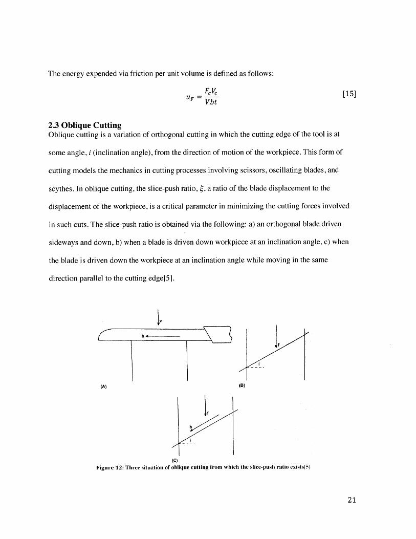
2.3 Oblique CuttingOblique cutting is a variation of orthogonal cutting in which the cutting edge of the tool is at
some angle, i (inclination angle), from the direction of motion of the workpiece. This form of
cutting models the mechanics in cutting processes involving scissors, oscillating blades, and
scythes. In oblique cutting, the slice-push ratio, , a ratio of the blade displacement to the
displacement of the workpiece, is a critical parameter in minimizing the cutting forces involved
in such cuts. The slice-push ratio is obtained via the following: a) an orthogonal blade driven
sideways and down, b) when a blade is driven down workpiece at an inclination angle, c) when
the blade is driven down the workpiece at an inclination angle while moving in the same
direction parallel to the cutting edge[5].
h
I
If
-ik
(C)
Figure 12: Three situation of oblique cutting from which the slice-push ratio existsl5l
21

2.3.1 Cutting ForcesFocusing on case a in Figure 11, a blade of angle, 0, experiences two displacements, a
movement, dh, parallel to the cutting edge and a displacement, dv, perpendicular to the
blades cutting edge.
Blade
.v- dhCos 0/
dh dr
dv
Figure 13: Pictorial representation of the displacements seen in an orthogonal blade moving parallel and normalto the cutting edge of the blade[5].
The resultant displacement of the offcut over the face of the tool can be defined using the
geometric relationships in Figure 11. Since the slice-push ratio is defined as the ratio of
these two displacements, the resultant displacement can be written using the slice-push
ratio.
dr = (dh)2 + (cos6) 2 + [16]
In oblique cutting, the two forces involved are Fv and H, and act parallel to the dv and dh,
respectively. During this cutting process, the work done for each increment of movement is
defined as the sum of the work expended in both directions of motion:
22
W =Vdv+ Hdh [17]
This incremental work is the amount of work required via fracture, which is defined as
Rwdv, where R is the specific work for surface separation of the material and w is the width
of the cut. As a result, the incremental work can be redefined as follows:
W = Vdv + Hdh = Rwdv [18]
When looking at the interface between the chip and the tool, the resultant force of friction
is acting in the same direction as the resultant displacement. Thus, the frictional work
expended for each displacement dr, is as follows, where p is the coefficient of friction and N
is the normal force acting on the tool face:
[19]Wf = Ndr
By substituting for dr and N, the force normal to the cutting edge, the incremental frictional
work is redefined as follows:
W = pVJ(scosO) 2 +1dv [20]f cosO(sinO+pcosO)
In equating the external and internal incremental works, the forces, Fv and H are defined as
follows:
Rw (1g-(y {oV ) (cos6(sinO+jysinO)) [2 1]
H RwV
Rw Rw [22]
23
2.3.2 Reciprocating BladesWhen dealing with reciprocating blades, the oscillations are defined as follows:
h = Asin(wt) [23]
During the reciprocation of the blade, as the workpiece is being feed to the tool, the slice-push
ratio changes in value. At the end of each oscillation the slice-push ratio become zero as the
blades comes to rest, and reaches a maximum value during the middle of the stroke. As result the
forces Fy and H become dependent on the oscillation of the blade. With this in mind the, slice-
push ratio, and the forces Fy and H can defined as follows:
h = AsinowtV V [24]
FV 1
Rw AA(sntoo 2 [25]S (1+sin&)t)2 -(2y +sinutcos (cose(sine+ysine))
H _ F sint [26]Rw Rw v
24
Chapter 3: Compliant StructuresCompliant structures are a wide subset of mechanical systems that utilize the elasticity of
systems to actuate systems small displacements via an applied force. A compliant flexural
mechanism is a single-pieced structure that incorporates flexures to provide motion in the desired
directions, while providing constraints in all others. These types of systems are favorable in
precision engineering because they allow for frictionless-movement for a controlled and limited
range. These systems can be found in many several systems, including atomic force microscopes
and optical equipment, and are a big area of interest in precision engineering[6].
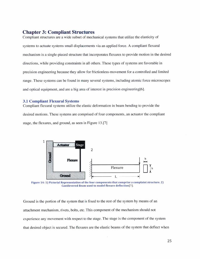
3.1 Compliant Flexural SystemsCompliant flexural systems utilize the elastic deformation in beam bending to provide the
desired motions. These systems are comprised of four components, an actuator the compliant
stage, the flexures, and ground, as seen in Figure 13.[7]
1
IT 2
Flexure h
L
Figure 14: 1) Pictorial Representation of the four components that comprise a complaint structure. 2)Cantilevered Beam used to model flexure deflection[7].
Ground is the portion of the system that is fixed to the rest of the system by means of an
attachment mechanism, rivets, bolts, etc. This component of the mechanism should not
experience any movement with respect to the stage. The stage is the component of the system
that desired object is secured. The flexures are the elastic beams of the system that deflect when
25
a force is applied in the desired direction, but restrict motion in all others. The actuator is the
device that provides the force.
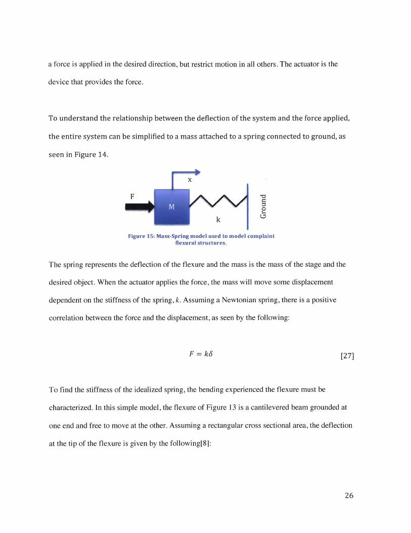
To understand the relationship between the deflection of the system and the force applied,
the entire system can be simplified to a mass attached to a spring connected to ground, as
seen in Figure 14.
X-
0
Figure 15: Mass-Spring model used to model complaintflexural structures.
The spring represents the deflection of the flexure and the mass is the mass of the stage and the
desired object. When the actuator applies the force, the mass will move some displacement
dependent on the stiffness of the spring, k. Assuming a Newtonian spring, there is a positive
correlation between the force and the displacement, as seen by the following:
F = kS [27]
To find the stiffness of the idealized spring, the bending experienced the flexure must be
characterized. In this simple model, the flexure of Figure 13 is a cantilevered beam grounded at
one end and free to move at the other. Assuming a rectangular cross sectional area, the deflection
at the tip of the flexure is given by the following[8]:
26
s FL [28]3EI
-1 [29]
E is the young's modulus of the material the flexure is composed of. The stiffness of the flexure
can be derived by rearranging S:
k 3E0 L[30]
All compliant flexural systems can be simplified into a mass and spring model. The math
however, will vary depending on the complexity of the system.
3.2 Piezoelectric ActuatorsWhen utilizing compliant flexural systems, the selection of the actuator is a critical step in
the design of the system. For small-scale systems, due to limitations in space, a small
actuator that can provide sufficient force to move stiff stages is required. Piezoelectric
actuators are often the choice of actuators for such systems. There are several types of
piezoelectric actuators, including stacks, plates, or benders, as shown in Figure 15.
27
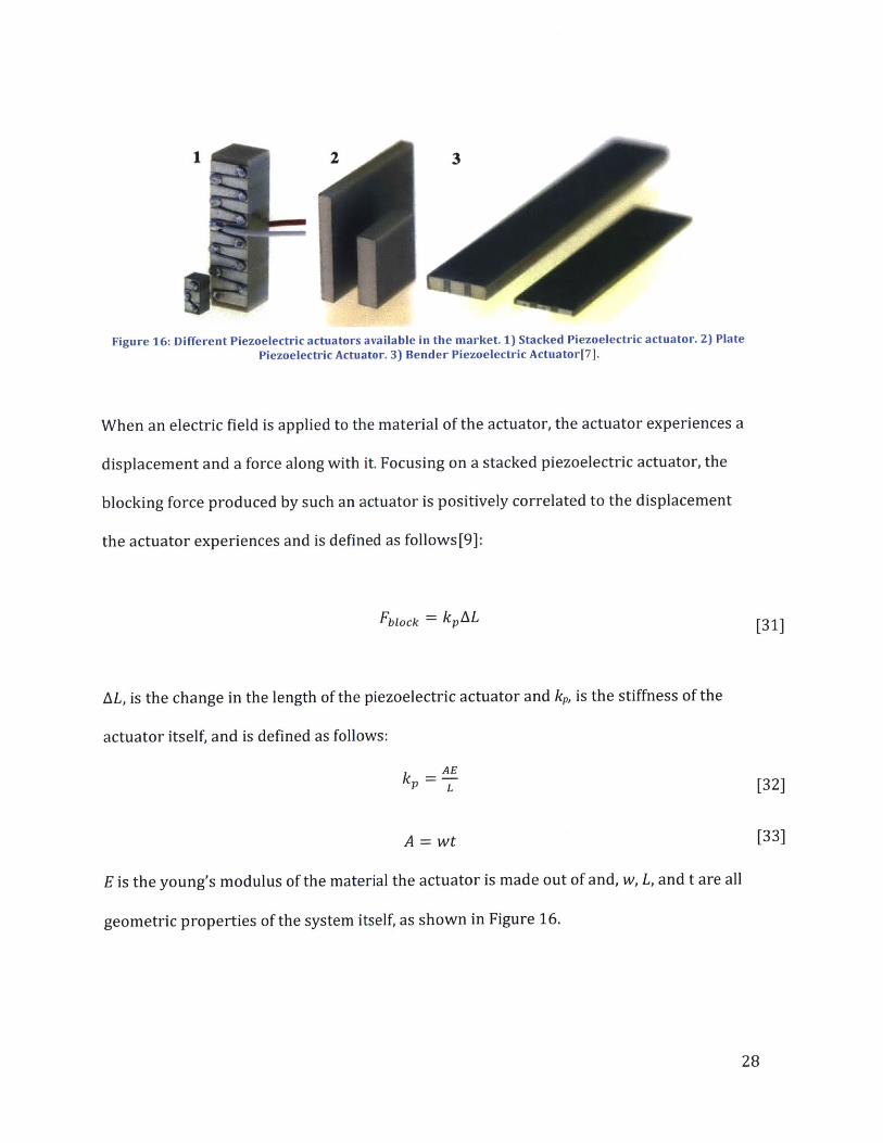
Figure 16: Different Piezoelectric actuators available in the market. 1) Stacked Piezoelectric actuator. 2) Plate
Piezoelectric Actuator. 3) Bender Piezoelectric Actuator[7].
When an electric field is applied to the material of the actuator, the actuator experiences a
displacement and a force along with it. Focusing on a stacked piezoelectric actuator, the
blocking force produced by such an actuator is positively correlated to the displacement
the actuator experiences and is defined as follows [9]:
Fblock = kPAL [31]
AL, is the change in the length of the piezoelectric actuator and kp, is the stiffness of the
actuator itself, and is defined as follows:
k = [32]
A =wt [33]
E is the young's modulus of the material the actuator is made out of and, w, L, and t are all
geometric properties of the system itself, as shown in Figure 16.
28
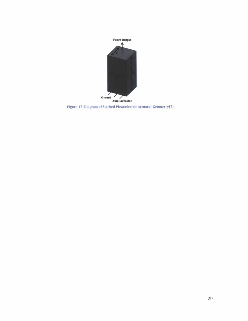
ForceOutputA
GroAxialActuator
Figure 17: Diagram of Stacked Piezoelectric Actuator Geometry[71.
29

Chapter 4: Assessment of Design and Theory
4.1 Vibrating Flexural Stage Design
4.1.1 Design SpecificationsA flexural stage that oscillated at a frequency,f,, and an amplitude, A, was explored as a
possible design to incorporate oscillations in ultramicrotomes. In order for the stage to run
properly it needed to adhere to the requirements in Table 4.1.
Table 1: Comparison of the Desire design specifications to the actual design specifications.
Driving Frequency 1000-2000 Hz 1000-2000 Hz
SUMO in1,54 NI n 63 7Stiffness in Z 21.5 N/micron 16.5 N/micron
Natra FTqily 200 0 Hz 5270 Hz
4.1.2 Linear Stage DesignTo arrive to the optimal flexural design, FACT was implemented. By defining the freedom
space as a single line and the constraint space as five planes normal to the freedom space,
the following two concepts were conceived [10].
Figure: Final two concepts developed from
30
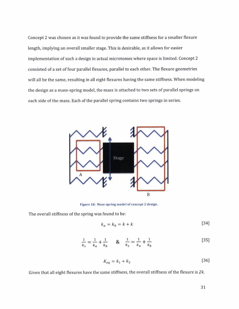
Concept 2 was chosen as it was found to provide the same stiffness for a smaller flexure
length, implying an overall smaller stage. This is desirable, as it allows for easier
implementation of such a design in actual microtomes where space is limited. Concept 2
consisted of a set of four parallel flexures, parallel to each other. The flexure geometries
will all be the same, resulting in all eight flexures having the same stiffness. When modeling
the design as a mass-spring model, the mass is attached to two sets of parallel springs on
each side of the mass. Each of the parallel spring contains two springs in series.
A
B
Figure 18: Mass-spring model of concept 2 design.
The overall stiffness of the spring was found to be:
ka=kb =k+k [34]
1 +1 & 1 +1 [35]k1 ka kb k 2 ka kb
Keq = k1 + k2 [36]
Given that all eight flexures have the same stiffness, the overall stiffness of the flexure is 2k.
31
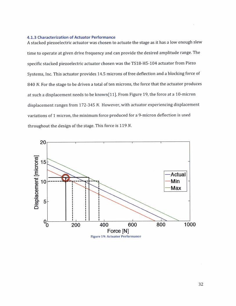
4.1.3 Characterization of Actuator PerformanceA stacked piezoelectric actuator was chosen to actuate the stage as it has a low enough slew
time to operate at given drive frequency and can provide the desired amplitude range. The
specific stacked piezoelectric actuator chosen was the TS18-H5-104 actuator from Piezo
Systems, Inc. This actuator provides 14.5 microns of free deflection and a blocking force of
840 N. For the stage to be driven a total of ten microns, the force that the actuator produces
at such a displacement needs to be known[11]. From Figure 19, the force at a 10-micron
displacement ranges from 172-345 N. However, with actuator experiencing displacement
variations of 1 micron, the minimum force produced for a 9-micron deflection is used
throughout the design of the stage. This force is 119 N.
20
15
10
5F
0'0
I I
I II II II II II II II II II II II II IIt I
200
-Act-Mir-Ma
400 600Force [N]
Figure 19: Actuator Performance
800
ual
1000
32
0
E
EZC0An5)
I
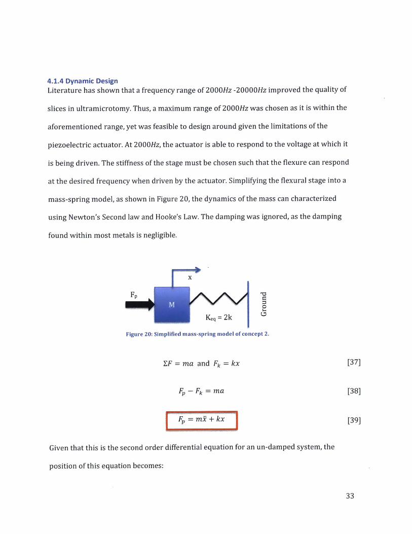
4.1.4 Dynamic DesignLiterature has shown that a frequency range of 2000Hz -20000Hz improved the quality of
slices in ultramicrotomy. Thus, a maximum range of 2000Hz was chosen as it is within the
aforementioned range, yet was feasible to design around given the limitations of the
piezoelectric actuator. At 2000Hz, the actuator is able to respond to the voltage at which it
is being driven. The stiffness of the stage must be chosen such that the flexure can respond
at the desired frequency when driven by the actuator. Simplifying the flexural stage into a
mass-spring model, as shown in Figure 20, the dynamics of the mass can characterized
using Newton's Second law and Hooke's Law. The damping was ignored, as the damping
found within most metals is negligible.
x0
Figure 20: Simplified mass-spring model of concept 2.
ZF = ma and Fk = kx [37]
Fp - Fk = ma [38]
F = MR + kx [39]
Given that this is the second order differential equation for an un-damped system, the
position of this equation becomes:
33
x(t) = Acos(wt) where & = J [40]
With the amplitude, A, being 10 microns, and the frequency, W, being 2000Hz, for a single
oscillation the position, x (at t =0.0005s), of the stage will be 0 microns. The mass of the
stage, m, is 0.0569 kg. Thus, k can be found by moving around the solution as follows:
k = m 7 [41]
Plugging in these values gives a stiffness of 0.5N/micron. With this stiffness being two
orders of magnitude lower than the maximum stiffness of the actuator (-80N/micron), the
output force of the actuator will be used in determining stiffness of the flexure.
For a 10-micron displacement, the output point force used is 119N. For the stage to operate
within the given design requirements, the stiffness must be within 0.5-80N/micron. In
operating the stage at the desired amplitude, a 10-micron offset is required. As such, the
stiffness of the stage must not be such that piezoelectric actuator is unable to provide
sufficient force to displace the stage an additional 10 microns. The stiffness, however,
cannot be so low that unforeseen errors via machining/installation will cause the stiffness
to be below the minimum threshold of 0.5N/microns. Thus, a stiffness of 5N/microns was
chosen, as it provided a force of 50 N onto the stage, while still being 10 times larger than
the minimum threshold accounting for any errors that might occur.
34

4.1.5: Flexural Stage Design
40 0
200
7!$T 1cw 47 All Dimension inmm
25.4
Figure 21: Final Design of Stage Design Values presented are valued measured post-fabrication
Figure 21, shows the final stage design with the critical part features labeled. The exact
stiffness (-4.69 N/micron) of the system was determined via finite element analysis. Slots
where machined into the sides of the stage to allow for installation of a sensor and actuator.
4.1.6: Actuator ConnectionInstallation of the actuator required that the actuator experienced no shear during
operation of the stage, as any shear would cause the PZT material fail. As a result, rounded
ends were attached to the end of the actuator to ensure that if any shear were to occur the
ballpoint contact would allow rolling at the intersection. For the stage to operate within the
required specifications, it was determined that a 10-micron offset with a stiffness of
5N/micron was required. To introduce the 10-micron offset into the system, steel plates
are introduced at both ends of the actuator. Since the rounded tips introduce Hertzian
deformation, it is important to characterize such deformation. For a ball-to-plate contact
the Hertzian deformation is defined as follows:
35

1
(9F2E) 6 (9F2)3[42]\2Re~e
where Ee = 106 GPa & Re = 1000 mm
With a 10-micron offset and a stiffness of 5 N/micron, the maximum force required by the
actuator during one oscillation is 100 N. Thus, a maximum 6.78 microns of Hertzian
deformation is expected to occur. Figure 22, is a pictorial representation of the actuator
assembly.
MA.A: Length of
-o4-
D: Thickness ofGlue
Thickness of Plate
Figure 22: Pictorial Representation of Actuator Assembly.
In determining the thickness of the steel plates, the following variables in Figure 22, along
with the Hertzian deformation were used. The thickness of the bonding agent was used
experimentally to be 79 microns. Compression experienced by the bonding agent was
neglected as the molecular composition of the epoxy prevents the material from
compressing for small thicknesses; these results were verified experimentally as well.
Thus, the following relationship was determined:
C + 0.01mm = A + 2B + 2D - 2 6 Hertz [42]
36
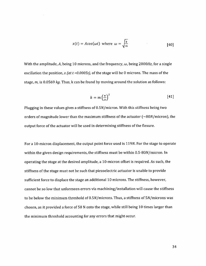
Solving for D, the plate thickness required was 0.989 mm. Figure 23, shows the final
assembled actuator.
Figure 22: Final assembled actuator installed into stage.
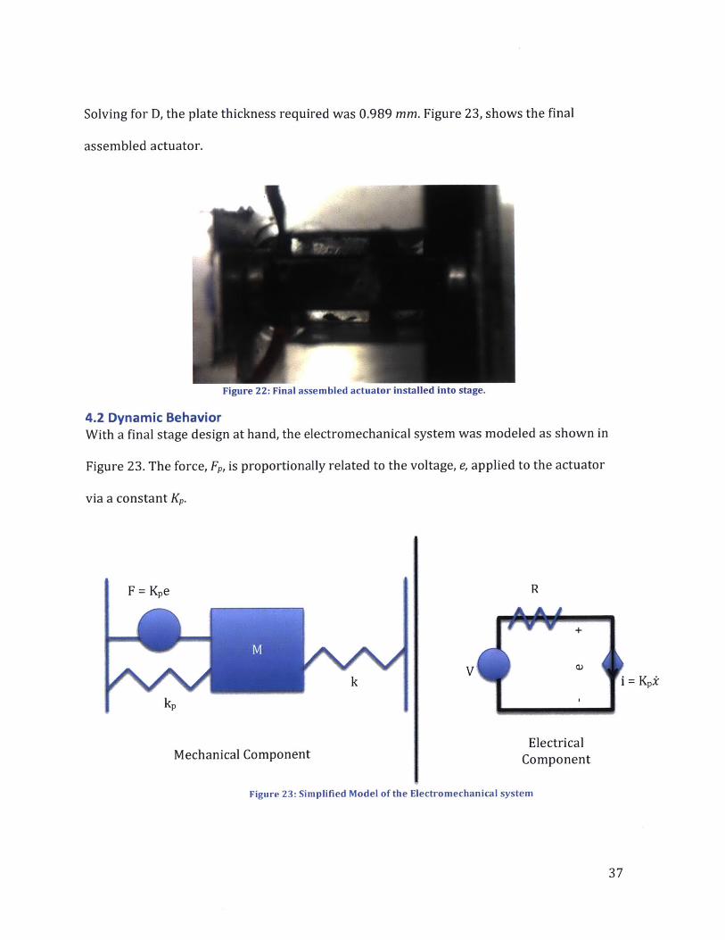
4.2 Dynamic BehaviorWith a final stage design at hand, the electromechanical system was modeled as shown in
Figure 23. The force, Fp, is proportionally related to the voltage, e, applied to the actuator
via a constant Kp.
F=Kpe
IA
Mechanical
EU V{k V
EComponent Co
Figure 23: Simplified Model of the Electromechanical system
R
Kpi
lectricalmponent
37
Using Hooke's Law and Newton's second law, the position of the mass, can be characterized
as follows:
EF = ma [43]
Fk = kx [44]
F - F- Fpiezo = ma [45]
FP = my + (k + kp)x [46]
Given the relationship of the actuator force to the voltage, e, the force of the actuator can be
defined as follows:
F = Kp(V - KpRi) [47]
Plugging this relationship into the differential equation for the un-damped second order
system becomes a damped, as shown:
KPV = mA + K2Rk + (k + kp)x [48]
where a) = k+kp & , = Kp R [49] [50]m 2mwn
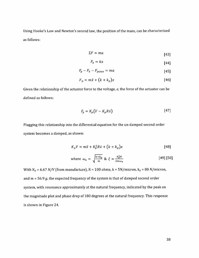
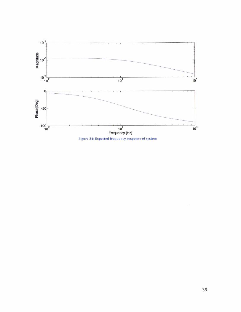
With Kp = 6.67 N/V (from manufacture), R = 100 ohms, k = 5N/micron, kp = 80 N/micron,
and m = 56.9 g, the expected frequency of the system is that of damped second order
system, with resonance approximately at the natural frequency, indicated by the peak on
the magnitude plot and phase drop of 180 degrees at the natural frequency. This response
is shown in Figure 24.
38
1u
10
0-10~ 2 104
10 101
-50
-100 2 3 410 10 10
Frequency [Hz]
Figure 24: Expected frequency response of system
39
Chapter 5: Validation of Design
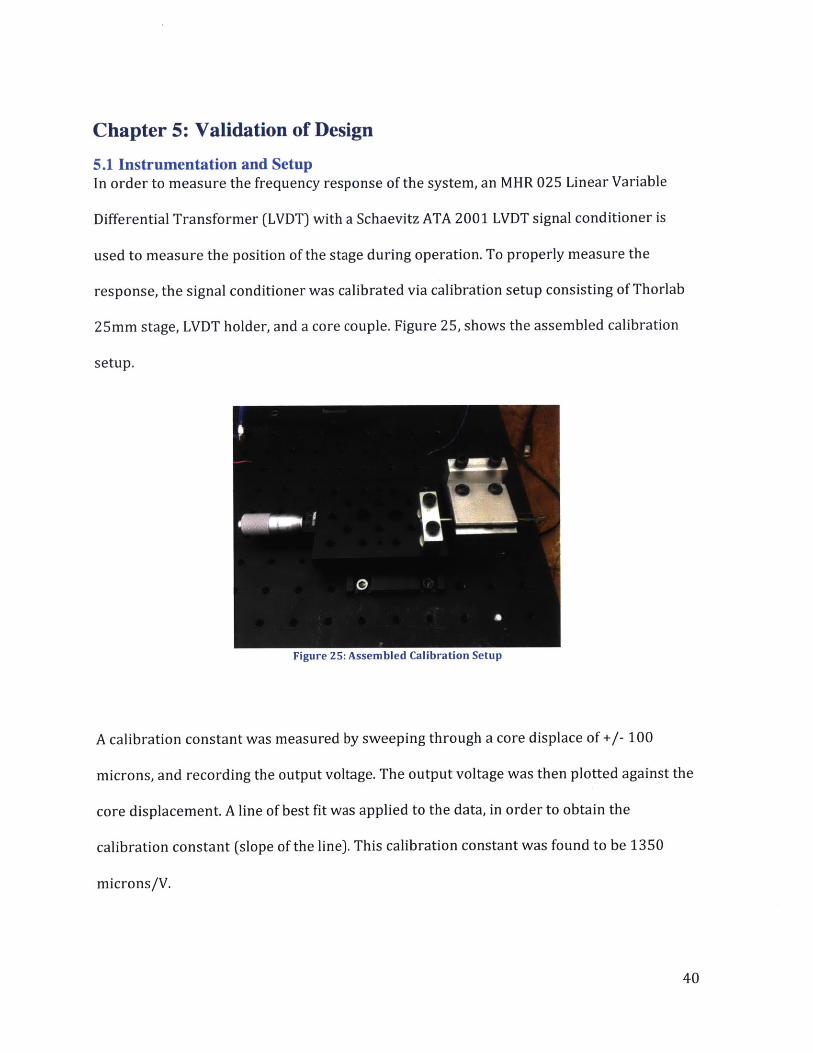
5.1 Instrumentation and SetupIn order to measure the frequency response of the system, an MHR 025 Linear Variable
Differential Transformer (LVDT) with a Schaevitz ATA 2001 LVDT signal conditioner is
used to measure the position of the stage during operation. To properly measure the
response, the signal conditioner was calibrated via calibration setup consisting of Thorlab
25mm stage, LVDT holder, and a core couple. Figure 25, shows the assembled calibration
setup.
Figure 25: Assembled Calibration Setup
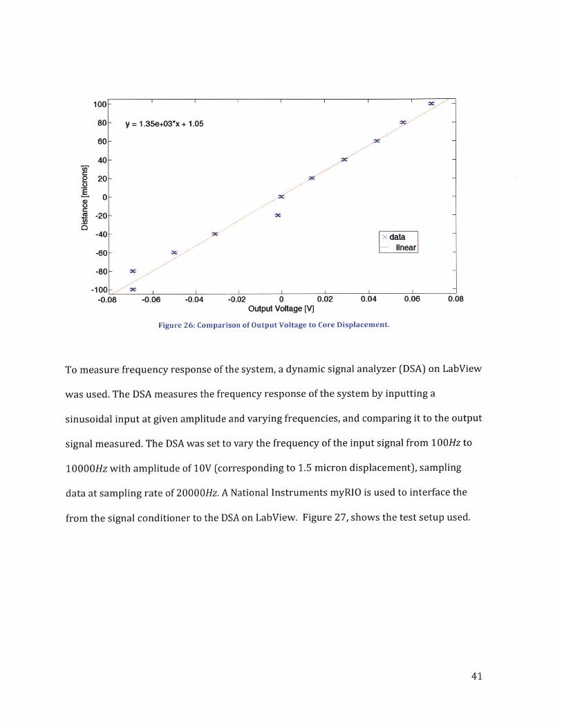
A calibration constant was measured by sweeping through a core displace of +/- 100
microns, and recording the output voltage. The output voltage was then plotted against the
core displacement. A line of best fit was applied to the data, in order to obtain the
calibration constant (slope of the line). This calibration constant was found to be 1350
microns/V.
40
100 - -
80- y =1.35e+03*x + 1.05
60 -- X-
40-
020-
E 0-
-20-
0--40 x data-
-60- linear
-60--80 - -
-100 - -I
-0.08 -0.06 -0.04 -0.02 0 0.02 0.04 0.06 0.08Output Voltage [V]
Figure 26: Comparison of Output Voltage to Core Displacement.
To measure frequency response of the system, a dynamic signal analyzer (DSA) on LabView
was used. The DSA measures the frequency response of the system by inputting a
sinusoidal input at given amplitude and varying frequencies, and comparing it to the output
signal measured. The DSA was set to vary the frequency of the input signal from 100Hz to
10000Hz with amplitude of 10V (corresponding to 1.5 micron displacement), sampling
data at sampling rate of 20000Hz. A National Instruments myRIO is used to interface the
from the signal conditioner to the DSA on LabView. Figure 27, shows the test setup used.
41
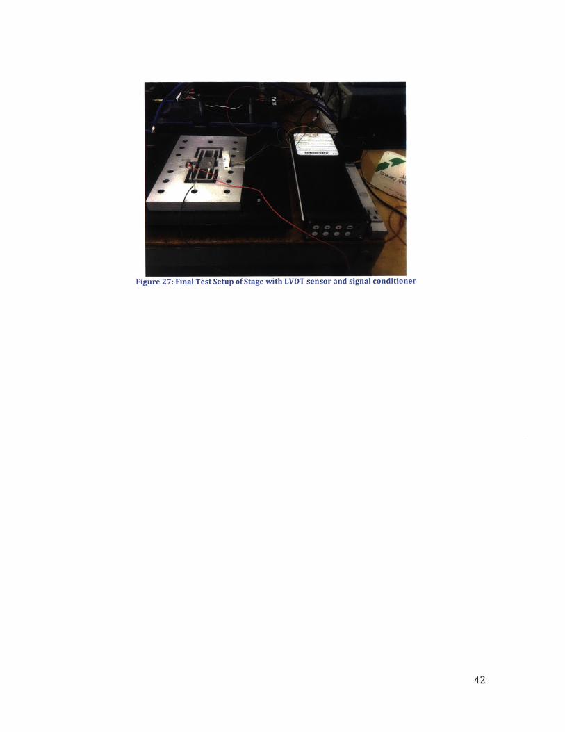
Figure 27: Final Test Setup of Stage with LVDT sensor and signal conditioner
42

Chapter 6: Results & Discussion
6.1: Experimental ResultsThe measured frequency response is shown in Figure 28. Comparing the expected
frequency response to the measured response, the expected damping of the system is much
higher than what is measured. In addition, the system experiences higher order resonances
occurring after the first peak that was not modeled in the expected response. Thus, a new
model was created to provide to better approximate behavior of the system.
1000
ib-5
i1010
00
0.
5001
-Measure Response-Expected Response
)2 10 3Frequency [Hz]
Figure 28:Comparison of Expected Response to Measured Response
1
1
To characterize the fitted model, a series of pairs of poles and zeros were placed in series of
each. Each pair of pole and zero is defined as follows:
Gpole = 121 _)S2+Lf[51]
43
............ ....... ....... ....... .... ... ...... 7 ....7 7 ... .....
4
04
2

Gzero 2)s2 + 2s +1 [52]
The natural frequencies were determined from the measured frequency response. The
damping ratio was iterated until the model fitted the measured response. In addition to
these poles and zeros, the +2 slope before the first resonance frequency indicates that two
zeros are present at the origin of the s-plane. Finally, a gain of 2.25x10⁸ is added to align
the measured magnitude response to the fitted response. The fitted model is compared to
the measured response in Figure 29. The fit provides an approximately good fit to the data.
There seems to be some deviation of the fit from the measured response in the phase
response. This deviation is caused by the low signal-to-noise ratio created by the small
voltage output of the signal conditioner. Because the minimum voltage the myRIO could
read was -1 mV, the output voltage of the signal conditioner (ranging ~ +/- 5mV)
produced a very low signal-to-noise ratio when read by the myRIO.
The transfer function of the model consists of three pairs of zeros and four pairs of poles,
and is shown as follows:
2.25*1 o 8s 2 (2.5*10-7 s2+7.5*10- 5s+1)(6.2 SE10~8 s2+4.5*10-5s+1)(2.77*10~8s2+3* 10~ 5 s+1))Gpit = ((*10-6)S2+0.0001s+1)(1.11*10-6S2+7.33*10-5s+1)(4*10-8s2+4*10-ss+1)(2.04*10-8s2+7.414*10-SS+1) [53]
44
10
1 0
10 02 10 3
500
0-Measured Response
0Fft
-500 2 310 10
Frequency [Hz]Figure 29: Comparison Fitted Model to Measured Response
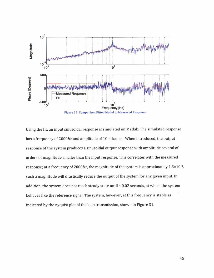
Using the fit, an input sinusoidal response is simulated on Matlab. The simulated response
has a frequency of 2000Hz and amplitude of 10 microns. When introduced, the output
response of the system produces a sinusoidal output response with amplitude several of
orders of magnitude smaller than the input response. This correlates with the measured
response; at a frequency of 2000Hz, the magnitude of the system is approximately 1.3x10 3 ,
such a magnitude will drastically reduce the output of the system for any given input. In
addition, the system does not reach steady state until -0.02 seconds, at which the system
behaves like the reference signal. The system, however, at this frequency is stable as
indicated by the nyquist plot of the loop transmission, shown in Figure 31.
45

1
-10.005 0.01 0.015 0.02 0.025 0.03
Time [seconds]
Figure 30: Simulated Input compared against output
0.035 0.04
response of system
i IT
-0.8 -0.6 -0.4 -0.2-0.8 -0.6 -0.4 -0.2
Real Axis
Figure 31: Nyquist plot of fitted model.
0 0.2 0.4
0-
CO
0R~ Reference
8Ouput Response8--
4 -
2 --
0 - -
-2- 1 -
-4- -t
-8-I It
0 0.045 0.05
0.04
0.03-
0.02-
. 0.01x
CM
0,
.g-0.01
-0.02-
-0.03-
-0.04-1
46

For the stage to be used in oscillatory cutting, the system needs a controller that increases
the magnitude of the system at the desired driven frequency, while still maintaining a
phase margin above zero (> 45 degrees to account for any unforeseen disturbances in the
system that might shift operating frequency) and a high enough crossover frequency (at
least an order of magnitude higher than 2000Hz to ensure that bandwidth of system is
sufficiently high enough). It should also be noted that the measured response is very noisy,
possibly creating responses in the system that do not exist. To improve on the data, the
output of the signal conditioner needs to be amplified to higher voltage to obtain better
results from the DSA from LabView. This can be done by means of a more sensitive LVDT or
use of capacitance that produces output signals in volts for micron-level displacements.
47
Chapter 7: ConclusionA flexural stage was designed with a stiffness of 4.69N/micron. The measured frequency
response of the system indicates three resonance peaks at 1000Hz, 3000Hz, and 5000Hz.
The stage met all of the desired design requirements. A fitted transfer function was shown
to provide a good model of the measured frequency response, deviating slightly at higher
frequencies. Using the fitted model, a simulated response was introduced and the output
response of the system was shown to have the same frequency, but the amplitude was
several orders of magnitude smaller. A controller is needed in order to improve the
performance of the device.
7.1 Future Work
7.1.1: Characterization of Flexural Stage DesignThis research only dealt with measuring the frequency response of a flexural stage that
characterized the desired performance for a stage in use in ultramicrotomy. In order to
integrate this flexural stage design into ultramicrotomy, a smaller unit must be built and
studied. Further characterization of the model's response to external disturbances, must be
studied to ensure that stage can perform to desired specifications.
7.1.2: Implementation of a ControllerGiven the performance of the system, a controller needs to be designed to improve the
performance of the system. Thus, amplification of the output signal from the signal
conditioner needs to be implemented in order to provide a more accurate measured
response.
48

Bibliography[1] Al-Amoudi, A., Studer, D., and Dubochet, J., 2005, "Cutting artefacts and cutting process
in vitreous sections for cryo-electron microscopy," J. Struct. Biol., 150(1), pp. 109-121.[2] Studer, and Gnaegi, 2000, "Minimal compression of ultrathin sections with use of an
oscillating diamond knife," J. Microsc., 197(1), pp. 94-100.[3] Gu, H., Zhang, J., Faucher, S., and Zhu, S., 2010, "Controlled chattering?a new 'cutting-
edge' technology for nanofabrication," Nanotechnology, 21(35), p. 355302.[4] Shaw, M. C., 2005, Metal cutting principles, Oxford University Press, New York.[5] Atkins, A. G., 2009, The science and engineering of cutting the mechanics and
processes of separating, scratching and puncturing biomaterials, metals and non-metals, Butterworth-Heinemann/Elsevier, Amsterdam; Boston.
[6] Thomas, M., 2015,"http://web.mit.edu/mact/www/Blog/Flexures/FlexureIndex.html."
[7] Monti, J., "Boundary Condition Effects On Vibrating Cantilever Beams," MIT.[8] Gere, J. M., and Goodno, B. J., 2013, Mechanics of materials, Cengage Learning,
Stamford, CT.[9] PI INC., "Piezo Design: Fundamentals of Piezoelectric Actuation."[10] Hopkins, J. B., and Culpepper, M. L., 2010, "Synthesis of multi-degree of freedom,
parallel flexure system concepts via Freedom and Constraint Topology (FACT) - Part I:Principles," Precis. Eng., 34(2), pp. 259-270.
[11] Piezo Systems, INC, "LOW VOLTAGE PIEZOELECTRIC STACKS."
49