Embed Size (px)
Citation preview

arX
iv:1
104.
4144
v1 [
hep-
ph]
21
Apr
201
1
Flavor SU(3) symmetry and QCD factorization
in B → PP and PV decays
Hai-Yang Cheng∗ and Sechul Oh†
Institute of Physics, Academia Sinica, Taipei 115, Taiwan
(Dated: October 29, 2018)
Abstract
Using flavor SU(3) symmetry, we perform a model-independent analysis of charmless Bu,d(Bs) →
PP, PV decays. All the relevant topological diagrams, including the presumably subleading dia-
grams, such as the QCD- and EW-penguin exchange diagrams and flavor-singlet weak annihilation
ones, are introduced. Indeed, the QCD-penguin exchange diagram turns out to be important in
understanding the data for penguin-dominated decay modes. In this work we make efforts to bridge
the (model-independent but less quantitative) topological diagram or flavor SU(3) approach and
the (quantitative but somewhat model-dependent) QCD factorization (QCDF) approach in these
decays, by explicitly showing how to translate each flavor SU(3) amplitude into the corresponding
terms in the QCDF framework. After estimating each flavor SU(3) amplitude numerically using
QCDF, we discuss various physical consequences, including SU(3) breaking effects and some useful
SU(3) relations among decay amplitudes of Bs → PV and Bd → PV .
∗ Email: [email protected]† Email: [email protected]
1

I. INTRODUCTION
A large number of hadronic Bu,d decay events have been collected at the B factories
which enable us to make accurate measurements of branching fractions (BFs) and direct
CP asymmetries for many modes. With the advent of the LHCb experiment, a tremendous
amount of new experimental data on B decays is expected to be obtained. In particular,
various decay processes of heavier Bs and Bc mesons as well as very rare B decay modes are
expected to be observed.
In earlier works on hadronic decays of B mesons, the factorization hypothesis, based
on the color transparency argument, was usually assumed to estimate the hadronic matrix
elements which are inevitably involved in theoretical calculations of the decay amplitudes
for these processes. Under the factorization assumption, the matrix element of a four-quark
operator is expressed as a product of a decay constant and a form factor. Naive factorization
is simple but fails to describe color-suppressed modes. This is ascribed to the fact that color-
suppressed decays receive sizable nonfactorizable contributions that have been neglected in
naive factorization. Another issue is that the decay amplitude under naive factorization is
not truly physical because the renormalization scale and scheme dependence of the Wilson
coefficients ci(µ) are not compensated by that of the matrix element 〈M1M2|Oi|B〉(µ). In
the improved “generalized factorization” approach [1, 2], nonfactorizable effects are absorbed
into the parameter N effc , the effective number of colors. This parameter can be empirically
determined from experiment.
With the advent of heavy quark effective theory, nonleptonic B decays can be analyzed
systematically within the QCD framework. There are three popular approaches available in
this regard: QCD factorization (QCDF) [3], perturbative QCD (pQCD) [4] and soft-collinear
effective theory (SCET) [5]. In QCDF and SCET, power corrections of order ΛQCD/mb are
often plagued by the end-point divergence that in turn breaks the factorization theorem. As
a consequence, the estimate of power corrections is generally model dependent and can only
be studied in a phenomenological way. In the pQCD approach, the endpoint singularity is
cured by including the parton’s transverse momentum.
Because a reliable evaluation of hadronic matrix elements is very difficult in general, an
alternative approach which is essentially model independent is based on the diagrammatic
approach [6–8]. In this approach, the topological diagrams are classified according to the
2

topologies of weak interactions with all strong interaction effects included. Based on fla-
vor SU(3) symmetry, this model-independent analysis enables us to extract the topological
amplitudes and sense the relative importance of different underlying decay mechanisms.
When enough measurements are made with sufficient accuracy, we can extract the diagram-
matic amplitudes from experiment and compare to theoretical estimates, especially checking
whether there are any significant final-state interactions or whether the weak annihilation
diagrams can be ignored as often asserted in the literature. The diagrammatic approach
was applied to hadronic B decays first in [9]. Various topological amplitudes have been
extracted from the data in [10–13] after making some reasonable approximations.
Based on SU(3) flavor symmetry, the decay amplitudes also can be decomposed into linear
combinations of the SU(3)F amplitudes which are SU(3) reduced matrix elements [14–17].
This approach is equivalent to the diagrammatic approach when SU(3) flavor symmetry is
imposed to the latter.
In this work we make efforts to bridge these two different approaches, using QCDF and
flavor SU(3) symmetry, in Bu,d(Bs) → PP, PV decays. For this aim, we first introduce all
the relevant topological diagrams, including the presumably subleading diagrams, such as
the QCD- and EW-penguin exchange ones and flavor-singlet weak annihilation ones, some
of which turn out to be important especially in penguin-dominant decay processes. Then all
these decay modes are analyzed by using the intuitive topological diagrams and expressed in
terms of the SU(3)F amplitudes. Each SU(3)F amplitude is translated into the corresponding
terms in the framework of QCDF. Applying these relations, one can easily find the rather
sophisticated results of the relevant decay amplitudes calculated in the QCDF framework.
The magnitude and the strong phase of each SU(3)F amplitude are numerically estimated
in QCDF. We further discuss some examples of the applications, including the effects of
SU(3)F breaking and useful SU(3)F relations among decay amplitudes.
This paper is organized as follows. In Sec. II, we introduce topological quark diagrams
relevant to Bu,d(Bs) → PP, PV decays and the framework of QCDF. The explicit SU(3)F
decomposition of the decay amplitudes and the relations between the SU(3)F amplitudes
and the QCDF terms are presented. In Sec. III, we make a numerical estimation of the
SU(3)F amplitudes and discuss its consequences and some applications. Our conclusions are
given in Sec. IV.
3

II. FLAVOR SU(3) ANALYSIS AND QCD FACTORIZATION
It has been established sometime ago that a least model-dependent analysis of heavy
meson decays can be carried out in the so-called quark-diagram approach. 1 In this dia-
grammatic scenario, all two-body nonleptonic weak decays of heavy mesons can be expressed
in terms of six distinct quark diagrams [6–8]: 2 T , the color-allowed external W -emission
tree diagram; C, the color-suppressed internal W -emission diagram; E, the W -exchange
diagram; A, the W -annihilation diagram; P , the horizontal W -loop diagram; and V , the
vertical W -loop diagram. (The one-gluon exchange approximation of the P graph is the
so-called “penguin diagram”.) For the analysis of charmless B decays, one adds the variants
of the penguin diagram such as the electroweak penguin and the penguin annihilation and
singlet penguins, as will be discussed below. It should be stressed that these diagrams are
classified according to the topologies of weak interactions with all strong interaction effects
encoded, and hence they are not Feynman graphs. All quark graphs used in this approach
are topological and meant to have all the strong interactions included, i.e., gluon lines are
included implicitly in all possible ways. Therefore, analyses of topological graphs can provide
information on final-state interactions (FSIs).
In SU(3)F decomposition of the decay amplitudes for Bu,d(Bs) → M1M2 (with
M1M2 = P1P2, PV, V P ) modes [15], we represent the decay amplitudes in terms of
topological quark diagram contributions. The topological amplitudes which will be referred
to as SU(3)F amplitudes hereafter, corresponding to different topological quark diagrams,
as shown in Figs. 1-3, can be classified into three distinct groups as follows:
(i) Tree and penguin amplitudes
T : color-favored tree amplitude (equivalently, external W -emission),
C : color-suppressed tree amplitude (equivalently, internal W -emission),
P : QCD-penguin amplitude,
S : singlet QCD-penguin amplitude involving SU(3)F-singlet mesons (e.g., η(′), ω, φ),
PEW : color-favored EW-penguin amplitude,
PCEW : color-suppressed EW-penguin amplitude,
1 It is also referred to as the flavor-flow diagram or topological-diagram approach in the literature.2 Historically, the quark-graph amplitudes T, C, E, A, P named in [15] were originally denoted by
A, B, C, D, E, respectively, in [7, 8].
4

(ii) Weak annihilation amplitudes
E : W -exchange amplitude,
A : W -annihilation amplitude,
(E and A are often jointly called “weak annihilation”.)
PE : QCD-penguin exchange amplitude,
PA : QCD-penguin annihilation amplitude,
PEEW : EW-penguin exchange amplitude,
PAEW : EW-penguin annihilation amplitude,
(PE and PA are also jointly called “weak penguin annihilation”.)
(iii) Flavor-singlet weak annihilation amplitudes: all involving SU(3)F-singlet mesons 3
SE : singlet W -exchange amplitude,
SA : singlet W -annihilation amplitude,
SPE : singlet QCD-penguin exchange amplitude,
SPA : singlet QCD-penguin annihilation amplitude,
SPEEW : singlet EW-penguin exchange amplitude,
SPAEW : singlet EW-penguin annihilation amplitude.
Within the framework of QCD factorization [20], the effective Hamiltonian matrix ele-
ments for B → M1M2 (M1M2 = P1P2, PV ) are written in the form
〈M1M2|Heff |B〉 = GF√2
∑
p=u,c
λrp 〈M1M2|TA
p + TBp|B〉 , (1)
where the Cabibbo-Kobayashi-Maskawa (CKM) factor λrp ≡ VpbV
∗pr with r = s, d. TA
p de-
scribes contributions from naive factorization, vertex corrections, penguin contractions and
spectator scattering expressed in terms of the flavor operators api , while TBp contains an-
nihilation topology amplitudes characterized by the annihilation operators bpj . The flavor
operators api are basically the Wilson coefficients in conjunction with short-distance nonfac-
torizable corrections such as vertex corrections and hard spectator interactions. In general,
they have the expressions [20, 21]
api (M1M2) =(
ci +ci±1
Nc
)
Ni(M2) +ci±1
Nc
CFαs
4π
[
Vi(M2) +4π2
Nc
Hi(M1M2)]
+ P pi (M2) , (2)
3 The singlet amplitudes SE and SA were first discussed in [18, 19] as the disconnected hairpin amplitudes
and denoted by Eh and Ah, respectively, in [19].
5

(a) T (b) C
(c) P, PCEW (d) S, PEW
W W
W
g
W
gg
B
B
B
B
M1
M2
M1
M2
M1
M2
M1
M2
FIG. 1: Topology of possible diagrams: (a) Color-allowed tree [T ], (b) Color-suppressed tree [C],
(c) QCD-penguin [P ], (d) Singlet QCD-penguin [S] diagrams with 2 (3) gluon lines for M2 being
a pseudoscalar meson P (a vector meson V ). The color-suppressed EW-penguin [PCEW] and color-
favored EW-penguin [PEW] diagrams are obtained by replacing the gluon line from (c) and all the
gluon lines from (d), respectively, by a single Z-boson or photon line.
where i = 1, · · · , 10, the upper (lower) signs apply when i is odd (even), ci are the Wilson
coefficients, CF = (N2c − 1)/(2Nc) with Nc = 3, M2 is the emitted meson and M1 shares
the same spectator quark with the B meson. The quantities Ni(M2) = 0 or 1 for i = 6, 8
and M2 = V or else, respectively. The quantities Vi(M2) account for vertex corrections,
Hi(M1M2) for hard spectator interactions with a hard gluon exchange between the emitted
meson and the spectator quark of the B meson and Pi(M2) for penguin contractions.
The weak annihilation contributions to the decay B → M1M2 (M1M2 = P1P2, PV, V P )
can be described in terms of the building blocks bpj and bpj,EW :
GF√2
∑
p=u,c
λrp 〈M1M2|TB
p|B〉 = iGF√2
∑
p=u,c
λrp fBfM1fM2
∑
j
(djbpj + d′jb
pj,EW). (3)
The building blocks have the expressions [20]
b1 =CF
N2c
c1Ai1, bp3 =
CF
N2c
[
c3Ai1 + c5(A
i3 + Af
3) +Ncc6Af3
]
,
b2 =CF
N2c
c2Ai1, bp4 =
CF
N2c
[
c4Ai1 + c6A
f2
]
,
bp3,EW =CF
N2c
[
c9Ai1 + c7(A
i3 + Af
3) +Ncc8Ai3
]
,
6

(e) E (f) A
(g) PE, PEEW (h) PA, PAEW
W
g
W
gg
g
g
W
W g
B
B
B
B
M1
M2
M1
M2
M1
M2
M1
M2
FIG. 2: (e) W -exchange [E], (f) W -annihilation [A], (g) QCD-penguin exchange [PE], (h) QCD-
penguin annihilation [PA] diagrams. The EW-penguin exchange [PEEW] and EW-penguin anni-
hilation [PAEW] diagrams are obtained from (g) and (h), respectively, by replacing the left gluon
line by a single Z-boson or photon line. The gluon line of (e) and (f) and the right gluon line of
(g) and (h) can be attached to the fermion lines in all possible ways.
bp4,EW =CF
N2c
[
c10Ai1 + c8A
i2
]
. (4)
The subscripts 1,2,3 of Ai,fn denote the annihilation amplitudes induced from (V −A)(V −A),
(V − A)(V + A) and (S − P )(S + P ) operators, respectively, and the superscripts i and f
refer to gluon emission from the initial and final-state quarks, respectively. We choose the
convention that M1 contains an antiquark from the weak vertex and M2 contains a quark
from the weak vertex, as in Ref. [21].
For the explicit expressions of vertex, hard spectator corrections and annihilation con-
tributions, we refer to [20–22] for details. In practice, it is more convenient to express the
decay amplitudes in terms of the flavor operators αpi and the annihilation operators βp
j which
are related to the coefficients api and bpj by
α1(M1M2) = a1(M1M2) , α2(M1M2) = a2(M1M2) ,
αp3(M1M2) =
ap3(M1M2)− ap5(M1M2) for M1M2 = PP, V P ,
ap3(M1M2) + ap5(M1M2) for M1M2 = PV ,
7

(i) SE (j) SA
(k) SPE, SPEEW (l) SPA, SPAEW
W
g
W
W
g
Wg
g
g
g
B
B
B
B
M1
M2
M1
M2
M1
M2
M1
M2
FIG. 3: (i) Flavor-singlet W -exchange [SE], (j) Flavor-singlet W -annihilation [SA], (k) Flavor-
singlet QCD-penguin exchange [SPE], (l) Flavor-singlet QCD-penguin annihilation [SPA] dia-
grams. The Flavor-singlet EW-penguin exchange [SPEEW] and flavor-singlet EW-penguin annihi-
lation [SPAEW] diagrams are obtained from (k) and (l), respectively, by replacing the leftest gluon
line by a single Z-boson or photon line. The double gluon lines of (i), (j), (k) and (l) are shown
for the case of M1 = P . They are replaced by three gluon lines when M1 = V . Each of the gluon
lines of (i), (j), (k) and (l) can be separately attached to the fermion lines in all possible ways.
αp4(M1M2) =
ap4(M1M2) + rM2χ ap6(M1M2) for M1M2 = PP, PV ,
ap4(M1M2)− rM2χ ap6(M1M2) for M1M2 = V P ,
(5)
αp3,EW(M1M2) =
ap9(M1M2)− ap7(M1M2) for M1M2 = PP, V P ,
ap9(M1M2) + ap7(M1M2) for M1M2 = PV ,
αp4,EW(M1M2) =
ap10(M1M2) + rM2χ ap8(M1M2) for M1M2 = PP, PV ,
ap10(M1M2)− rM2χ ap8(M1M2) for M1M2 = V P ,
and
βpj (M1M2) =
ifBfM1fM2
X(BM1,M2)bpj (M1M2) , (6)
where fM is the decay constant of a meson M and the chiral factors rM2χ are given by
rPχ (µ) =2m2
P
mb(µ)(m2 +m1)(µ), rVχ (µ) =
2mV
mb(µ)
f⊥V (µ)
fV, (7)
8

with f⊥V (µ) being the scale-dependent transverse decay constant of the vector meson V . The
relevant factorizable matrix elements are
X(BP1,P2) ≡ 〈P2|Jµ|0〉〈P1|J ′µ|B〉 = ifP2(m
2B −m2
P1) FBP1
0 (m2P2) ,
X(BP,V ) ≡ 〈V |Jµ|0〉〈P |J ′µ|B〉 = 2fV mBpc F
BP1 (m2
V ) ,
X(BV,P ) ≡ 〈P |Jµ|0〉〈V |J ′µ|B〉 = 2fP mBpc A
BV0 (m2
P ) , (8)
with pc being the c.m. momentum. Here we have followed the conventional Bauer-Stech-
Wirbel definition for form factors FBP0,1 and ABV
0 [23].
A. SU(3)F decomposition of decay amplitudes
The decay amplitudes of Bu,d(Bs) → M1M2 modes can be analyzed by the relevant quark
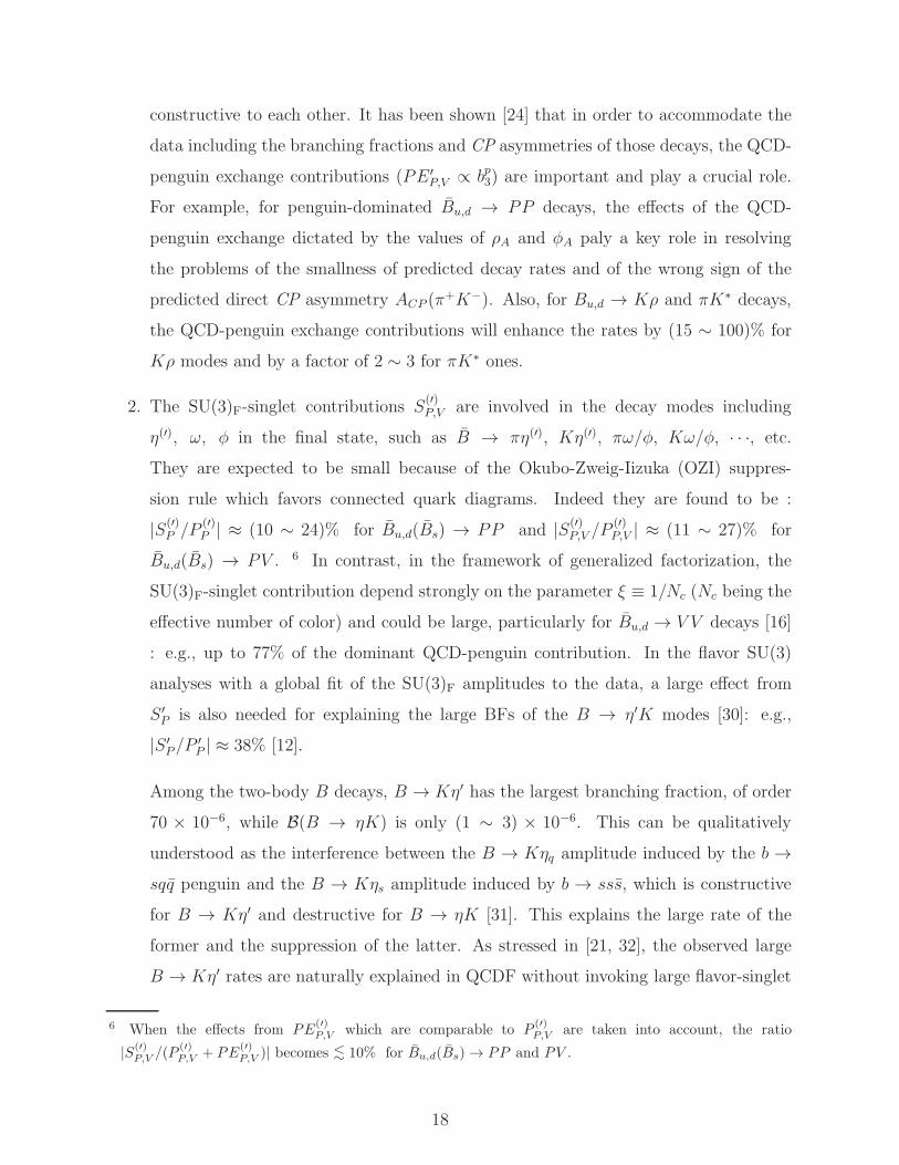
diagrams and written in terms of the SU(3)F amplitudes. The decomposition of the decay
amplitudes of these modes is displayed in Tables I−XXIV. In these tables, the subscript
M1 (or M2) of the amplitudes T(ζ)M1 [M2]
, · · ·, etc., represents the case that the meson M1 (or
M2) contains the spectator quark in the final state. The superscript ζ of the amplitudes is
only applied to the case involving an η(′) or an ω/φ, or both η(′) and ω/φ in the final state
and denotes the quark content (ζ = q, s, c) of η(′) and ω/φ with q = u or d. The value of
ζ is shown in the parenthesis as (q), (s) or (c). For B0(Bs) → η(′)η(′), two values of ζ are
shown in one parenthesis: e.g., (q, s), where q and s denote the quark content of the first
and second η(′), respectively. A similar rule is also applied to the case of B0(Bs) → η(′) ω/φ.
On the other hand, to distinguish the decays with |∆S| = 1 from those with ∆S = 0,
we will put the prime to all the SU(3)F amplitudes for the former, for example T′(ζ)M1 [M2]
.
The SU(3)F-singlet amplitudes S(′)M1[M2]
are involved only when the SU(3)F-singlet meson(s)
(η, η′, ω, φ) appear(s) in the final state.
We will give some examples for illustration. The decay amplitude of B− → π−K0 which
is a Bu → PP mode with |∆S| = 1 can be written, from Tables IV−V, as
AB−→π−K0 = P ′π −
1
3PC′EW,π + A′
π + PE ′π +
2
3PE ′
EW,π . (9)
The decay amplitude of B0 → η(′)K∗0 which is a Bd → PV mode with |∆S| = 1 can be
recast, from Tables X−XII, to
√2 AB0→η(′)K∗0
9

=(
C′(q)K∗ + 2S
′(q)K∗ +
1
3P
′(q)EW, K∗ + 2SPE
′(q)K∗ − 2
3SPE
′(q)EW, K∗
)
+√2(
S′(s)K∗ + P
′(s)K∗ − 1
3P
′(s)EW, K∗ − 1
3P
C′, (s)EW, K∗ + PE
′(s)K∗ − 1
3PE
′(s)EW, K∗
+SPE′(s)K∗ − 1
3SPE
′(s)EW, K∗
)
+√2(
C′(c)K∗ + S
′(c)K∗
)
+(
P′(q)η(′)
− 1
3P
C′, (q)
EW, η(′)+ PE
′(q)η(′)
− 1
3PE
′(q)EW, η(′)
)
, (10)
where the superscripts (q), (s) and (c) represent the quark contents of η(′), such as η(′)q , η(′)s
and η(′)c , respectively. Likewise, from Tables VII−IX, the decay amplitude of B0 → η(′) ω/φ
which is a Bd → PV mode with ∆S = 0 is given by
2 AB0→η(′) ω/φ =(
C(q, q)
η(′)+ 2S
(q, q)
η(′)+ P
(q, q)
η(′)+
1
3P
(q, q)
EW, η(′)− 1
3P
C, (q, q)
EW, η(′)
+E(q, q)
η(′)+ PE
(q, q)
η(′)+ 2PA
(q, q)
η(′)− 1
3PE
(q, q)
EW, η(′)+
1
3PA
(q, q)
EW, η(′)
+2SE(q, q)
η(′)+ 2SPE
(q, q)
η(′)+ 4SPA
(q, q)
η(′)− 2
3SPE
(q, q)
EW, η(′)+
2
3SPA
(q, q)
EW, η(′)
)
+√2(
S(q, s)
η(′)− 1
3P
(q, s)
EW, η(′)+ SE
(q, s)
η(′)+ SPE
(q, s)
η(′)+ 2SPA
(q, s)
η(′)
−1
3SPE
(q, s)
EW, η(′)+
1
3SPA
(q, s)
EW, η(′)
)
+√2(
2SPA(s, q)
η(′)− 2
3SPA
(s, q)
EW, η(′)
)
+ 2(
PA(s, s)
η(′)− 1
3PA
(s, s)
EW, η(′)+ SPA
(s, s)
η(′)− 1
3SPA
(s, s)
EW, η(′)
)
+(
C(q, q)ω/φ + 2S
(q, q)ω/φ + P
(q, q)ω/φ +
1
3P
(q, q)EW, ω/φ −
1
3P
C, (q, q)EW, ω/φ
+E(q, q)ω/φ + PE
(q, q)ω/φ + 2PA
(q, q)ω/φ − 1
3PE
(q, q)EW, ω/φ +
1
3PA
(q, q)EW, ω/φ
+2SE(q, q)ω/φ + 2SPE
(q, q)ω/φ + 4SPA
(q, q)ω/φ − 2
3SPE
(q, q)EW, ω/φ +
2
3SPA
(q, q)EW, ω/φ
)
+√2(
S(q, s)ω/φ − 1
3P
(q, s)EW, ω/φ + SE
(q, s)ω/φ + SPE
(q, s)ω/φ + 2SPA
(q, s)ω/φ
−1
3SPE
(q, s)EW, ω/φ +
1
3SPA
(q, s)EW, ω/φ
)
+√2(
C(q, c)ω/φ + S
(q, c)ω/φ
)
+√2(
2SPA(s, q)ω/φ − 2
3SPA
(s, q)EW, ω/φ
)
+ 2(
PA(s, s)ω/φ − 1
3PA
(s, s)EW, ω/φ + SPA
(s, s)ω/φ − 1
3SPA
(s, s)EW, ω/φ
)
, (11)
where the superscripts (q′, q′′) with q′, q′′ = q, s denote the quark contents of (η(′), ω/φ),
such as (η(′)q , ωq/φq), (η(′)q , ωs/φs), etc. When ideal mixing for ω and φ is assumed, ωs and
10

φq terms vanish: i.e., the amplitudes with the superscripts (q, s) or (s, s) for B → η(′)ω
and the superscripts (q, q) or (s, q) for B → η(′)φ are set to be zero.
B. The SU(3)F amplitudes and QCD factorization
The SU(3)F amplitudes for Bu,d(Bs) → M1M2 (with M1M2 = P1P2, PV, V P ) decays
can be expressed in terms of the quantities calculated in the framework of QCD factorization
as follows: 4
T(ζ)M1[M2]
=GF√2
λru α1(M1M2) X
(BM1, M2) [X(BM2, M1)] ,
C(ζ)M1[M2]
=GF√2
λru α2(M1M2) X
(BM1, M2) [X(BM2, M1)] ,
S(ζ)M1[M2]
=GF√2
∑
p=u,c
λrp αp
3(M1M2) X(BM1, M2) [X(BM2, M1)] ,
P(ζ)M1[M2]
=GF√2
∑
p=u,c
λrp αp
4(M1M2) X(BM1, M2) [X(BM2, M1)] ,
P(ζ)EW,M1[M2]
=GF√2
∑
p=u,c
λrp
3
2αp3,EW(M1M2) X
(BM1, M2) [X(BM2, M1)] ,
PC, (ζ)EW,M1[M2]
=GF√2
∑
p=u,c
λrp
3
2αp4,EW(M1M2) X
(BM1, M2) [X(BM2, M1)] , (12)
where the superscript ζ = q, s, c, which is only applied to the case when M1 (or M2) = η(′)
or ω/φ, or M1M2 = η(′)η(′) or η(′)ω/φ. As mentioned before, for |∆S| = 1 decays, we will
put the prime to all the SU(3)F amplitudes. The unprimed and primed amplitudes have
the CKM factor λrp ≡ VpbV
∗pr with r = d and r = s, respectively. The weak annihilation
amplitudes are given by
E(ζ)M1[M2]
=GF√2λru (ifBfM1fM2) [b1]M1M2 [M2M1]
,
A(ζ)M1[M2]
=GF√2λru (ifBfM1fM2) [b2]M1M2 [M2M1]
,
PE(ζ)M1[M2]
=GF√2
∑
p=u,c
λrp (ifBfM1fM2) [bp3]M1M2 [M2M1]
,
PA(ζ)M1[M2]
=GF√2
∑
p=u,c
λrp (ifBfM1fM2) [bp4]M1M2 [M2M1]
,
PE(ζ)EW,M1[M2]
=GF√2
∑
p=u,c
λrp (ifBfM1fM2)
[
3
2bp3,EW
]
M1M2 [M2M1],
4 The factorizable amplitude X(BM1, M2) is denoted by AM1M2in [21].
11

PA(ζ)EW,M1[M2]
=GF√2
∑
p=u,c
λrp (ifBfM1fM2)
[
3
2bp4,EW
]
M1M2 [M2M1], (13)
and the singlet weak annihilation amplitudes by
SE(ζ)M1[M2]
=GF√2λru (ifBfM1fM2) [bS1]M1M2 [M2M1]
,
SA(ζ)M1[M2]
=GF√2λru (ifBfM1fM2) [bS2]M1M2 [M2M1]
,
SPE(ζ)M1[M2]
=GF√2
∑
p=u,c
λrp (ifBfM1fM2) [bpS3]M1M2 [M2M1]
,
SPA(ζ)M1[M2]
=GF√2
∑
p=u,c
λrp (ifBfM1fM2) [bpS4]M1M2 [M2M1]
,
SPE(ζ)EW,M1[M2]
=GF√2
∑
p=u,c
λrp (ifBfM1fM2)
[
3
2bpS3,EW
]
M1M2 [M2M1],
SPA(ζ)EW,M1[M2]
=GF√2
∑
p=u,c
λrp (ifBfM1fM2)
[
3
2bpS4,EW
]
M1M2 [M2M1], (14)
where we have used the notation [bpj ]M1M2 ≡ bpj (M1,M2). Note that the weak annihilation
contributions in the QCDF approach given in Eq. (3) include all the above SU(3)F amplitudes
given in Eqs. (13) and (14), such as E(′)Mi, A
(′)Mi, . . . , SE
(′)Mi, SA
(′)Mi, · · ·, etc.
Using the above relations, one can easily translate the decay amplitude expressed in
terms of the SU(3)F amplitudes as shown in Tables I−XXIV into that expressed in terms
of the quantities calculated in the framework of QCDF. For example, the decay amplitude
of B− → π−K0 given in Eq. (9) can be rewritten in terms of the quantities calculated in
QCDF:
AB−→π−K0 =GF√2
∑
p=u,c
λsp
[
δpu β2 + αp4 −
1
2αp4,EW + βp
3 + βp3,EW
]
X(Bπ, K) . (15)
Likewise, the decay amplitude of B0 → η(′)K∗0 in Eq. (10) now reads
√2 AB0→η(′)K∗0
=GF√2
∑
p=u,c
λsp
{
[
δpu α2 + 2αp3 +
1
2αp3,EW + βp
3 + βp3,EW
]
X(BK∗, η(′)q )
+√2[
αp3 + αp
4 −1
2αp3,EW − 1
2αp4,EW + βp
3 −1
2βp3,EW + βp
S3 −1
2βpS3,EW
]
X(BK∗, η(′)s )
+√2[
δpc α2 + αp3
]
X(BK∗, η(′)c )
+[
αp4 −
1
2αp4,EW + βp
3 −1
2βp3,EW
]
X(Bη(′)q , K∗)
}
. (16)
12

Finally, the decay amplitude of B0 → η(′) ω/φ in Eq. (11) is recast to
2 AB0→η(′) ω/φ
=GF√2
∑
p=u,c
λdp
{
[
δpu (α2 + β1 + 2βS1) + 2αp3 + αp
4 +1
2αp3,EW − 1
2αp4,EW
+βp3 + 2βp
4 −1
2βp3,EW +
1
2βp4,EW + 2βp
S3 + 4βpS4 − βp
S3,EW + βpS4,EW
]
X(Bη(′)q , ωq/φq)
+√2[
δpu βS1 + αp3 −
1
2αp3,EW + βS3 + 2βp
S4 −1
2βpS3,EW +
1
2βpS4,EW
]
X(Bη(′)q , ωs/φs)
+√2 (−ifBfη(′)fω/φ)
[
2bpS4 − bpS4,EW
]
η(′)s ωq/φq
+2 (−ifBfη(′)fω/φ)
[
bp4 −1
2bp4,EW + bpS4 −
1
2bpS4,EW
]
η(′)s ωs/φs
+[
δpu (α2 + β1 + 2βS1) + 2αp3 + αp
4 +1
2αp3,EW − 1
2αp4,EW
+βp3 + 2βp
4 −1
2βp3,EW +
1
2βp4,EW + 2βp
S3 + 4βpS4 − βp
S3,EW + βpS4,EW
]
X(B ωq/φq, η(′)q )
+√2[
δpu βS1 + αp3 −
1
2αp3,EW + βS3 + 2βp
S4 −1
2βpS3,EW +
1
2βpS4,EW
]
X(B ωq/φq , η(′)s )
+√2[
δpc α2 + αp3
]
X(B ωq/φq , η(′)c )
+√2 (−ifBfη(′)fω/φ)
[
2bpS4 − bpS4,EW
]
ωs/φs, η(′)q
+2 (−ifBfη(′)fω/φ)
[
bp4 −1
2bp4,EW + bpS4 −
1
2bpS4,EW
]
ωs/φs, η(′)s
}
. (17)
All the decay amplitudes of B → PP, V P in QCD factorization shown in Appendix A of
Ref. [21] can be obtained from the SU(3)F amplitudes displayed in Tables I−XXIV.
III. NUMERICAL ANALYSIS OF FLAVOR SU(3) AMPLITUDES IN QCDF
In this section we estimate the magnitude of each SU(3)F amplitude in the framework of
QCDF by using the relations given in Eqs. (12), (13) and (14). For the numerical analysis, we
shall use the same input values for the relevant parameters as those in Ref. [24]. Specifically
we use the values of the form factors for Bu,d → P and Bu,d → V transitions obtained in the
light-cone QCD sum rules [25] and those for Bs → V transitions obtained in the covariant
light-front quark model [26] with some modifications :
FBπ0 (0) = 0.25 , FBK
0 (0) = 0.35 , FBηq0 (0) = 0.296 ,
13

FBsK0 (0) = 0.24 , FBsηs
0 (0) = 0.28 ,
ABρ0 (0) = 0.303 , ABK∗
0 (0) = 0.374 , ABω0 (0) = 0.281 ,
ABsK∗
0 (0) = 0.30 , ABsφ0 (0) = 0.32 . (18)
Here for η(′) we have used the flavor states qq ≡ (uu+ dd)/√2, ss and cc labeled by the ηq,
ηs and ηc, respectively, and the form factors for B → η(′) are given by
FBη = FBηq cos θ , FBη′ = FBηq sin θ ,
FBsη = −FBsηs sin θ , FBsη′ = FBsηs cos θ , (19)
where the small mixing with ηc is neglected and the ηq-ηs mixing angle θ defined by
|η〉 = cos θ|ηq〉 − sin θ|ηs〉,
|η′〉 = sin θ|ηq〉+ cos θ|ηs〉, (20)
is (39.3 ± 1.0)◦ in the Feldmann-Kroll-Stech mixing scheme [27]. For the decay constants,
we use the values (in units of MeV) [27, 28]
fπ = 132 , fK = 160 , fBu,d= 210 , fBs
= 230 ,
f qη′ = 107 , f q
η = 89 , f sη′ = −112 , f s
η = 137 ,
fρ = 216 , fK∗ = 220 , fω = 187 , fφ = 215 . (21)
It is known that although physics behind nonleptonic B decays is extremely complicated,
it is greatly simplified in the heavy quark limit mb → ∞ as the decay amplitude becomes
factorizable and can be expressed in terms of decay constants and form factors. However, this
simple approach encounters three major difficulties: (i) the predicted branching fractions for
penguin-dominated B → PP, V P, V V decays are systematically below the measurements
[21] (ii) direct CP-violating asymmetries for B0 → K−π+, B0 → K∗−π+, B− → K−ρ0,
B0 → π+π− and B0s → K+π− disagree with experiment in signs [29], and (iii) the transverse
polarization fraction in penguin-dominated charmless B → V V decays is predicted to be
very small, while experimentally it is comparable to the longitudinal polarization one. All
these indicate the necessity of going beyond zeroth 1/mb power expansion. In the QCDF
approach one considers the power correction to penguin amplitudes due to weak penguin
annihilation characterized by the parameter βp3 or bp3. However, QCD-penguin exchange
14

amplitudes involve troublesome endpoint divergences and hence they can be studied only in
a phenomenological way. We shall follow [20] to model the endpoint divergence X ≡ ∫ 10 dx/x
in the annihilation diagrams as
XA = ln(
mB
Λh
)
(1 + ρAeiφA), (22)
where Λh is a typical scale of order 500 MeV, and ρA and φA are the unknown real parameters.
By adjusting the magnitude ρA and the phase φA in this scenario, all the above-mentioned
difficulties can be resolved. However, a scrutiny of the QCDF predictions reveals more puz-
zles with respect to direct CP violation, as pointed out in [24, 29]. While the signs of
CP asymmetries in K−π+, K−ρ0 modes are flipped to the right ones in the presence of
power corrections from penguin annihilation, the signs of ACP in B− → K−π0, K−η, π−η
and B0 → π0π0, K∗0η will also get reversed in such a way that they disagree with exper-
iment. This indicates that it is necessary to consider subleading power corrections other
than penguin annihilation. It turns out that an additional subleading 1/mb power cor-
rection to color-suppressed tree amplitudes is crucial for resolving the aforementioned CP
puzzles and explaining the decay rates for the color-suppressed tree-dominated π0π0, ρ0π0
modes [24, 29]. A solution to the B → Kπ CP-puzzle related to the difference of CP asym-
metries of B− → K−π0 and B0 → K−π+ requires a large complex color-suppressed tree
amplitude and/or a large complex electroweak penguin. These two possibilities can be dis-
criminated in tree-dominated B decays. The CP puzzles with π−η, π0π0 and the rate deficit
problems with π0π0, ρ0π0 can only be resolved by having a large complex color-suppressed
tree topology C. While the New Physics solution to the B → Kπ CP puzzle is interesting,
it is most likely irrelevant for tree-dominated decays.
We shall use the fitted values of the parameters ρA and φA given in [24]:
For Bu,d(Bs) → PP , ρA = 1.10 (1.00) , φA = −50◦ (−55◦) ,
For Bu,d(Bs) → V P , ρA = 1.07 (0.90) , φA = −70◦ (−65◦) ,
For Bu,d(Bs) → PV , ρA = 0.87 (0.85) , φA = −30◦ (−30◦) . (23)
Following [29], power corrections to the color-suppressed topology are parametrized as
a2 → a2(1 + ρCeiφC ), (24)
with the unknown parameters ρC and φC to be inferred from experiment. We shall use [29]
ρC ≈ 1.3 , 0.8 , 0, φC ≈ −70◦ ,−80◦ , 0, (25)
15

for B → PP, V P, V V decays, respectively.
A. Magnitudes and strong phases of the SU(3)F amplitudes
From Eqs. (12)−(14), it is obvious that the SU(3)F amplitudes for Bu,d(Bs) → M1M2
depend on the specific final states M1 and M2. Thus, the magnitudes of these SU(3)F
amplitudes are process-dependent in general, though numerically the dependence turns out
to be moderate. In order to find typical magnitudes of these SU(3)F ones, we choose typical
decay processes as explained below, and use only the central values of the input parameters.
¿From now on, we shall use a notation for the relevant strong and weak phases as follows:
e.g., the color-favored tree amplitude for ∆S = 0 (|∆S| = 1) decays is denoted as T(′)P ≡
|T (′)P | ei(δT (′)
P+θT (′)) with the strong phase δ
T (′)P and the weak phase θT (′) = arg(VubV
∗ud(s)).
The numerical estimates of the SU(3)F amplitudes are displayed in Tables XXV−XXVIII.
In the case of Bu,d(Bs) → P1P2 decays with ∆S = 0, the modes Bu,d(Bs) → ππ (πK) are
used to numerically compute the relevant SU(3)F amplitudes such as TP , CP , PP and so on,
except for S(q,s,c)P which Bu,d(Bs) → πη (Kη) are used for. Similarly, for |∆S| = 1 decays
the processes Bu,d(Bs) → πK (KK) are used to estimate T ′P , C
′P , P
′P and so on, except for
S′(q,s,c)P which Bu,d(Bs) → Kη (ηη) are used for. In the case of ∆S = 0 Bu,d(Bs) → PV
decays, the modes Bu,d(Bs) → πρ (πK∗, Kρ) are used for the numerical calculation of the
amplitudes TP,V , CP,V , PP,V and so on, except for S(q,s,c)P and S
(q,s,c)V for which Bu,d(Bs) →
πω/φ (Kω/φ) and ηρ (ηK∗), respectively, are used. For |∆S| = 1 decays the processes
Bu,d(Bs) → πK∗, Kρ (KK∗) are used to estimate T ′P,V , C
′P,V , P
′P,V and so on, except for
S′(q,s,c)P and S
′(q,s,c)V for which Bu,d(Bs) → Kω/φ (ηω/φ) and ηK∗ (ηφ), respectively, are
used. The strong phases of the SU(3)F amplitudes are generated from the flavor operators
αpi and bpj . As shown in Eqs. (12)−(14), except the amplitudes T (′), C(′), E(′), A(′), SE(′)
and SA(′), all the other amplitudes including penguin ones are the sum of two terms each
of which is proportional to λrpα
pi or λr
pbpj with p = u, c. Because the CKM factors λr
u and λrc
involve different weak phases from each other, to exhibit the strong phase of each amplitude
in the tables, we shall use the approximations, αu3,4(EW) ≃ αc
3,4(EW) and bu3,4(EW) ≃ bc3,4(EW),
where the former (latter) relation holds roughly (very well) in QCDF. 5 Thus, for instance,
5 In QCDF the value of αci (i = 3, 4, (3,EW), (4,EW)) differ from that of αu
i by about (25−30)%, while the
16

the QCD-penguin amplitude can be understood as P (′) ≡ −|P (′)|eiδP(′)
eiθP (′)
with the strong
phase δP(′)
and the weak phase θP(′)
= arg(VtbV∗td(s)).
From Tables XXV−XXVIII, hierarchies among the SU(3)F amplitudes are numerically
found as follows. For ∆S = 0 Bu,d(Bs) → PP decays, the hierarchical relation is
|TP | > |CP | > |PP | >∼ |PEP | > |EP | > |S(s)P | ∼ |S(q)
P | ∼ |PEW, P | ∼ |AP | ∼ |PAP |
> |PCEW, P | > |PEEW, P | ∼ |PAEW, P | ∼ |S(c)
P | , (26)
and for Bu,d(Bs) → PV ,
|TP,V | > |CP,V | > |PEP,V | >∼ |PP,V | ∼ |EP,V | > |PEW, P,V | >∼ |AP,V | ∼ |S(s)P,V | ∼ |S(q)
P,V |>∼ |PC
EW, P,V | > |PAP,V | >∼ |PEEW, P,V | >∼ |PAEW, P,V | ∼ |S(c)V | . (27)
Likewise, for ∆S = 1 Bu,d(Bs) → PP decays, the hierarchical relation is found to be
|P ′P | >∼ |PE ′
P | > |T ′P | >∼ |P ′
EW, P | >∼ |C ′P | >∼ |S ′(s)
P | ∼ |S ′(q)P | ∼ |PA′
P |
> |PC′EW, P | > |E ′
P | > |A′P | ∼ |PE ′
EW, P | ∼ |PA′EW, P | >∼ |S ′(c)
P | , (28)
and for Bu,d(Bs) → PV ,
|PE ′P,V | >∼ |P ′
P,V | > |T ′P,V | >∼ |P ′
EW, P,V | > |C ′P,V | ∼ |S ′(s)
P,V | ∼ |S ′(q)P,V | >∼ |PC′
EW, P,V |
> |PE ′EW, V | >∼ |PA′
P,V | ∼ |E ′P,V | > |A′
P,V | > |PE ′EW, P | ∼ |PA′
EW, P,V | ∼ |S ′(c)V | . (29)
Several remarks are in order:
1. It is well known that the penguin contributions are dominant in |∆S| = 1 decays due
to the CKM enhancement |VcsV∗cb| ≈ |VtsV
∗tb| ≫ |VusV
∗ub| and the large top quark mass.
Especially, it is interesting to note that in addition to the QCD-penguin contributions
P ′P,V , the QCD-penguin exchange ones PE ′
P,V are large for Bu,d(Bs) → PP and PV
decays. Since the strong phase of PE ′P (V ) is comparable to that of P ′
P (V ) in magnitude
with the same sign (i.e., δPE′P (V ) ∼ δP ′
P (V )), the effects from PE ′P (V ) and P ′
P (V ) are strongly
value of bci is the same as that of bui . It should be emphasized that using Eqs. (12)−(14), one can compute
both the magnitude and strong phase of each SU(3)F amplitude without invoking these approximations
on αu,ci and bu,ci . In our numerical analysis, we use these approximations only for expressing the strong
phases as shown in Tables XXV−XXVIII. All the magnitudes of the amplitudes are obtained without
using these approximations.
17
constructive to each other. It has been shown [24] that in order to accommodate the
data including the branching fractions and CP asymmetries of those decays, the QCD-
penguin exchange contributions (PE ′P,V ∝ bp3) are important and play a crucial role.
For example, for penguin-dominated Bu,d → PP decays, the effects of the QCD-
penguin exchange dictated by the values of ρA and φA paly a key role in resolving
the problems of the smallness of predicted decay rates and of the wrong sign of the
predicted direct CP asymmetry ACP (π+K−). Also, for Bu,d → Kρ and πK∗ decays,
the QCD-penguin exchange contributions will enhance the rates by (15 ∼ 100)% for
Kρ modes and by a factor of 2 ∼ 3 for πK∗ ones.
2. The SU(3)F-singlet contributions S(′)P,V are involved in the decay modes including
η(′), ω, φ in the final state, such as B → πη(′), Kη(′), πω/φ, Kω/φ, · · ·, etc.
They are expected to be small because of the Okubo-Zweig-Iizuka (OZI) suppres-
sion rule which favors connected quark diagrams. Indeed they are found to be :
|S(′)P /P
(′)P | ≈ (10 ∼ 24)% for Bu,d(Bs) → PP and |S(′)
P,V /P(′)P,V | ≈ (11 ∼ 27)% for
Bu,d(Bs) → PV . 6 In contrast, in the framework of generalized factorization, the
SU(3)F-singlet contribution depend strongly on the parameter ξ ≡ 1/Nc (Nc being the
effective number of color) and could be large, particularly for Bu,d → V V decays [16]
: e.g., up to 77% of the dominant QCD-penguin contribution. In the flavor SU(3)
analyses with a global fit of the SU(3)F amplitudes to the data, a large effect from
S ′P is also needed for explaining the large BFs of the B → η′K modes [30]: e.g.,
|S ′P/P
′P | ≈ 38% [12].
Among the two-body B decays, B → Kη′ has the largest branching fraction, of order
70 × 10−6, while B(B → ηK) is only (1 ∼ 3) × 10−6. This can be qualitatively
understood as the interference between the B → Kηq amplitude induced by the b →sqq penguin and the B → Kηs amplitude induced by b → sss, which is constructive
for B → Kη′ and destructive for B → ηK [31]. This explains the large rate of the
former and the suppression of the latter. As stressed in [21, 32], the observed large
B → Kη′ rates are naturally explained in QCDF without invoking large flavor-singlet
6 When the effects from PE(′)P,V which are comparable to P
(′)P,V are taken into account, the ratio
|S(′)P,V /(P
(′)P,V + PE
(′)P,V )| becomes <∼ 10% for Bu,d(Bs) → PP and PV .
18

contributions.
3. In ∆S = 0 decays, as expected, the tree contributions TP,V dominate and the color-
suppressed tree amplitudes CP,V are larger than the penguin ones. Among the pen-
guin contributions, the QCD-penguin ones PP,V and the QCD-penguin exchange ones
PEP,V are comparable. Large strong phases in the decay amplitudes are needed
to generate sizable direct CP violation in B decay processes. For tree-dominated
Bu,d(Bs) → PP decays we have CP/TP ≈ 0.63 e−i56◦ (0.83 e−i53◦) which is larger than
the naive expectation of CP/TP ∼ 1/3 in both magnitude and phase. Recall that
a large complex color-suppressed tree topology C is needed to solve the rate deficit
problems with π0π0 and π0ρ0 and give the correct sign for direct CP violation in the
decays K−π0, K−η, K∗0η, π0π0 and π−η [24].
4. The W -exchange E(′)P,V , W -annihilation A
(′)P,V and QCD-penguin annihilation PA
(′)P,V
contributions are small, as expected because of a helicity suppression factor of
fB/mB ≈ 5% arising from the smallness of the B meson wave function at the ori-
gin [15]; they are at most only a few % (or up to 12% in the case of PA′A) of the
dominant contributions TP,V or P ′P,V .
Finally let us compare the numerical values of the SU(3)F amplitudes computed in QCDF
with those obtained from global fits to charmless Bu,d → PP and Bu,d → PV decays.
The ratios of the SU(3)F amplitudes extracted from global fits to charmless Bu,d → PP
modes [12] are 7
∣
∣
∣
∣
∣
∣
C(′)P
T(′)P
∣
∣
∣
∣
∣
∣
= 0.67 (0.67),
∣
∣
∣
∣
∣
∣
P(′)P /λ
d(s)t
T(′)P /λ
d(s)u
∣
∣
∣
∣
∣
∣
= 0.17 (0.14),
∣
∣
∣
∣
∣
∣
S(′)P /λ
d(s)t
T(′)P /λ
d(s)u
∣
∣
∣
∣
∣
∣
= 0.065 (0.053),
∣
∣
∣
∣
∣
∣
P(′)EW,P/λ
d(s)t
T(′)P /λ
d(s)u
∣
∣
∣
∣
∣
∣
= 0.020 (0.016), (30)
with λrq ≡ VqbV
∗qr (q = u, t and r = d, s), and the relative strong phases are
δC(′)P − δ
T (′)P = −68.3◦ , δ
P (′)P − δ
T (′)P = −15.9◦ ,
δS(′)P − δ
T (′)P = −42.9◦ , δ
PEW(′)P − δ
T (′)P = −57.6◦ . (31)
7 We only show the cases of “Scheme 4” in [12] for Bu,d → PP and of “Scheme B2” in [13] for Bu,d → PV
below, since these cases take into account the largest set of SU(3) breaking effects among the four schemes
presented in [12] and [13]. For comparison to our results, only the central values are shown.
19

Likewise, for charmless Bu,d → PV modes, the ratios of the SU(3)F amplitudes extracted
from global fits [13] are∣
∣
∣
∣
∣
∣
C(′)P
T(′)P
∣
∣
∣
∣
∣
∣
= 0.15 (0.15),
∣
∣
∣
∣
∣
∣
C(′)V
T(′)V
∣
∣
∣
∣
∣
∣
= 0.76 (0.76),
∣
∣
∣
∣
∣
∣
P(′)P /λ
d(s)t
T(′)P /λ
d(s)u
∣
∣
∣
∣
∣
∣
= 0.11 (0.11),
∣
∣
∣
∣
∣
∣
P(′)V /λ
d(s)t
T(′)V /λ
d(s)u
∣
∣
∣
∣
∣
∣
= 0.056 (0.046),
∣
∣
∣
∣
∣
∣
S(′)P /λ
d(s)t
T(′)P /λ
d(s)u
∣
∣
∣
∣
∣
∣
= 0.018 (0.018),
∣
∣
∣
∣
∣
∣
S(′)V /λ
d(s)t
T(′)V /λ
d(s)u
∣
∣
∣
∣
∣
∣
= 0.041 (0.034),
∣
∣
∣
∣
∣
∣
P(′)EW,P/λ
d(s)t
T(′)P /λ
d(s)u
∣
∣
∣
∣
∣
∣
= 0.039 (0.039),
∣
∣
∣
∣
∣
∣
P(′)EW,V /λ
d(s)t
T(′)V /λ
d(s)u
∣
∣
∣
∣
∣
∣
= 0.074 (0.061), (32)
and the relative strong phases are
δC(′)P − δ
T (′)P = 149.0◦ , δ
T (′)V − δ
T (′)P = 0.6◦ , δ
C(′)V − δ
T (′)P = −75.9◦ ,
δP (′)P − δ
T (′)P = −2.6◦ , δ
P (′)V − δ
T (′)P = 172.5◦ ,
δS(′)P − δ
T (′)P = −139.8◦ , δ
S(′)V − δ
T (′)P = −47.7◦ ,
δPEW(′)P − δ
T (′)P = 59.0◦ , δ
PEW(′)V − δ
T (′)P = −111.0◦ . (33)
In the above the numerical values outside (inside) parentheses correspond to ∆S = 0 (|∆S| =1) decays. In the case of Bu,d → PP with |∆S| = 1, the primed amplitudes were obtained
by including the SU(3) breaking factor fK/fπ for both |T ′P | and |C ′
P | and a universal SU(3)
breaking factor ξ = 1.04 for all the amplitudes except P ′EW,P. But, in Bu,d → PV , the
primed amplitudes were extracted by imposing partial SU(3) breaking factors on T and C
only: i.e., including fK∗/fρ for |T ′P | and |C ′
P |, and fK/fπ for |T ′V | and |C ′
V |. Also, for both
Bu,d → PP and PV , the top penguin dominance was assumed, which is equivalent to the
assumption that αu3,4(EW) ≃ αc
3,4(EW) in QCDF. For the strong phases, exact flavor SU(3)
symmetry was assumed in the fits so that δTP = δT ′P , δCP = δC′
P , etc. In Bu,d → PV , all the
relative strong phases were found relative to the strong phase of TP (i.e., δTP ).
On the other hand, from Table XXV, the ratios of the SU(3)F amplitudes for Bu,d → PP
are given by∣
∣
∣
∣
∣
∣
C(′)P
T(′)P
∣
∣
∣
∣
∣
∣
= 0.63 (0.64),
∣
∣
∣
∣
∣
∣
P(′)P /λ
d(s)t
T(′)P /λ
d(s)u
∣
∣
∣
∣
∣
∣
= 0.091 (0.097),
∣
∣
∣
∣
∣
∣
S(′)(q)P /λ
d(s)t
T(′)P /λ
d(s)u
∣
∣
∣
∣
∣
∣
= 0.014 (0.012),
∣
∣
∣
∣
∣
∣
P(′)EW,P/λ
d(s)t
T(′)P /λ
d(s)u
∣
∣
∣
∣
∣
∣
= 0.013 (0.016),
20

∣
∣
∣
∣
∣
∣
PE(′)P /λ
d(s)t
T(′)P /λ
d(s)u )
∣
∣
∣
∣
∣
∣
= 0.061 (0.060), (34)
and the relative strong phases are
δC(′)P − δ
T (′)P = −55.7◦ (−57.5◦) , δ
P (′)P − δ
T (′)P = −158.6◦ (−158.3◦) ,
δS(′)(q)
P − δT (′)P = 158.2◦ (149.4◦) , δ
PEW(′)P − δ
T (′)P = −179.8◦ (−179.8◦) ,
δPE(′)P − δ
T (′)P = −147.1◦ (−147.1◦) . (35)
Likewise, for Bu,d → PV , we obtain
∣
∣
∣
∣
∣
∣
C(′)P
T(′)P
∣
∣
∣
∣
∣
∣
= 0.30 (0.35),
∣
∣
∣
∣
∣
∣
C(′)V
T(′)V
∣
∣
∣
∣
∣
∣
= 0.39 (0.33),
∣
∣
∣
∣
∣
∣
P(′)P /λ
d(s)t
T(′)P /λ
d(s)u
∣
∣
∣
∣
∣
∣
= 0.030 (0.036),
∣
∣
∣
∣
∣
∣
P(′)V /λ
d(s)t
T(′)V /λ
d(s)u
∣
∣
∣
∣
∣
∣
= 0.041 (0.039),
∣
∣
∣
∣
∣
∣
S(′)P /λ
d(s)t
T(′)P /λ
d(s)u
∣
∣
∣
∣
∣
∣
= 0.005 (0.006),
∣
∣
∣
∣
∣
∣
S(′)V /λ
d(s)t
T(′)V /λ
d(s)u
∣
∣
∣
∣
∣
∣
= 0.010 (0.007),
∣
∣
∣
∣
∣
∣
P(′)EW,P/λ
d(s)t
T(′)P /λ
d(s)u
∣
∣
∣
∣
∣
∣
= 0.014 (0.019),
∣
∣
∣
∣
∣
∣
P(′)EW,V /λ
d(s)t
T(′)V /λ
d(s)u
∣
∣
∣
∣
∣
∣
= 0.013 (0.014),
∣
∣
∣
∣
∣
∣
PE(′)P /λ
d(s)t
T(′)P /λ
d(s)u
∣
∣
∣
∣
∣
∣
= 0.037 (0.040),
∣
∣
∣
∣
∣
∣
PE(′)V /λ
d(s)t
T(′)V /λ
d(s)u
∣
∣
∣
∣
∣
∣
= 0.051 (0.049), (36)
and the relative strong phases are
δC(′)P − δ
T (′)P = −16.8◦ (−19.8◦) , δ
C(′)V − δ
T (′)P = −52.5◦ (−56.2◦) ,
δP (′)P − δ
T (′)P = −145.5◦ (−145.2◦) , δ
P (′)V − δ
T (′)P = 7.6◦ (7.1◦) ,
δS(′)P − δ
T (′)P = −5.5◦ (−6.4◦) , δ
S(′)V − δ
T (′)P = 150.7◦ (133.4◦) ,
δPEW(′)P − δ
T (′)P = 179.8◦ (179.8◦) , δ
PEW(′)V − δ
T (′)P = −179.7◦ (−179.7◦) ,
δPE(′)P − δ
T (′)P = −124.4◦ (−125.0◦) , δ
PE(′)V − δ
T (′)P = 4.5◦ (4.2◦) , (37)
where the numerical values outside (inside) parentheses correspond to ∆S = 0 (|∆S| = 1)
decays. In our case, δTP = δTV = δT ′P = δT ′
V .
In comparison of Eqs. (30)−(33) [“fitting case”] with Eqs. (34)−(37) [“QCDF case”], it
is found that the values of |C(′)P /T
(′)P | for Bu,d → PP in the fitting case are very similar
to those of our QCDF case: both results show the large magnitudes of C(′)P together with
large strong phases, as discussed in the above “remark 3”. But, for Bu,d → PV , the values
21

of |C(′)P,V /T
(′)P,V | from both cases are different: in the fitting case, the ratios |C(′)
V /T(′)V | are
significantly larger than |C(′)P /T
(′)P |, though the values of |C(′)
P | include large errors in [13],
while in the QCDF case |C(′)V /T
(′)V | ∼ |C(′)
P /T(′)P |. For the penguin amplitudes, the results from
both cases are also different. The values of |(P (′)P /λ
d(s)t )/(T
(′)P /λd(s)
u )| for both Bu,d → PP
and PV in the fitting case are larger than those in the QCDF case. In the latter case,
the effects from PE(′)P are comparable to and contribute constructively to those of P
(′)P , as
discussed in the above “remark 1”. Interestingly it is found that the combined effects from
P(′)P and PE
(′)P obtained in the QCDF case are comparable to that of P
(′)P determined in
the fitting case. In contrast, the combined effects from P(′)V and PE
(′)V found in the QCDF
case are (roughly two times) larger than that of P(′)P obtained in the fitting case. Also,
for Bu,d → PV decays, the ratio |(P (′)P /λ
d(s)t )/(T
(′)P /λd(s)
u )| ∼ |(P (′)V /λ
d(s)t )/(T
(′)V /λd(s)
u )| in the
QCDF case, while |(P (′)P /λ
d(s)t )/(T
(′)P /λd(s)
u )| ∼ 2|(P (′)V /λ
d(s)t )/(T
(′)V /λd(s)
u )| in the fitting case.
For the SU(3)F-singlet contributions, as discussed in the above “remark 2”, S(′)P,V obtained
in the fitting case are much larger than those found in the QCDF case: e.g., for Bu,d → PV ,
the ratio |S(′)V /P
(′)V | ≈ 73% in the fitting case, in contrast to |S(′)
V /(P(′)V + PE
(′)V )| <∼ 10% [or
|S(′)V /P
(′)V | ≈ (18− 24)%] in the QCDF case.
B. Estimates of decay amplitudes, SU(3)F breaking effects and SU(3)F relations
Using Tables XXV−XXVIII, one can easily estimate the decay amplitudes of Bu,d(Bs) →PP, PV numerically. For example, the decay amplitude of B− → π−π0 is obtained as
√2AB−→π−π0 = Tπ + Cπ + PEW,π + PC
EW,π
= (1.52− i 24.94)× 10−9 GeV , (38)
and the decay amplitude of B− → π−K0 given in Eq. (9) is estimated as
AB−→π−K0 = (−49.71− i 24.77)× 10−9 GeV . (39)
Likewise, the decay amplitude of Bs → K0π0 is found to be
ABs→K0π0 = CK − PK + PEW,K +1
3PCEW,K − PEK +
1
3PEEW,K
= (−16.32− i 17.91)× 10−9 GeV , (40)
22

and the decay amplitude of Bs → K+K∗− is given by
ABs→K+K∗− = T ′K + P ′
K +2
3PC′EW,K + E ′
K∗ + PE ′K + PA′
K + PA′K∗
−1
3PE ′
EW,K − 1
3PA′
EW,K +2
3PE ′
EW,K∗
= (−30.20− i 4.97)× 10−9 GeV . (41)
In the above, the color-suppressed and color-favored tree amplitudes are, for example, CK ≡|CK | ei(δ
CK+θC) and T ′
K ≡ |T ′K | ei(δ
T ′K
+θT ′), respectively, with the strong phases δCK and δT ′K and
the weak phases θC = arg(VubV∗ud) and θT ′ = arg(VubV
∗us). The QCD- and EW-penguin and
weak annihilation amplitudes have the similar form, such as P(′)K ≡ |P (′)
K | ei(δP (′)K
+θP (′)) and
EK∗ ≡ |E ′K∗| ei(δE′
K∗+θE′), etc, where the strong phases δPK 6= δP ′K 6= δE′
K∗ in general and the
weak phases θP = arg( − VtbV∗td) and θP ′ = θE′ = arg( − VtbV
∗ts). By using Eqs. (38)−(41),
and noting that each SU(3)F amplitude and its CP-conjugate one are the same except for
having the weak phase with opposite sign to each other (e.g., the CP-conjugate amplitude
to CK is |CK | ei(δCK−θC)), the estimation of direct CP asymmetries as well as the decay rates
can be easily obtained.
The SU(3)F breaking effects in the amplitudes arise from the decay constants, masses of
the mesons and the form factors in addition to the CKM matrix elements. For example,
taking into account the effects of SU(3)F breaking in Bu,d → PP , the ratio of T ′P and TP
is estimated by |T ′P/TP | ≈ [|Vus| fK(m2
B − m2K)F
BK0 ]/[|Vud| fπ(m2
B − m2π)F
Bπ0 ]. From Ta-
bles XXV−XXVIII, the numerical estimates of the SU(3)F breaking effects in the amplitudes
can be obtained. For both Bu,d(Bs) → PP decays with ∆S = 0 and |∆S| = 1,∣
∣
∣
∣
∣
Vud T ′P
Vus TP
∣
∣
∣
∣
∣
= 1.22 (1.21),
∣
∣
∣
∣
∣
Vud C ′P
Vus CP
∣
∣
∣
∣
∣
= 1.25 (1.26),
∣
∣
∣
∣
∣
Vtd P ′P
Vts PP
∣
∣
∣
∣
∣
= 1.18 (1.18),
∣
∣
∣
∣
∣
Vtd PE ′P
Vts PEP
∣
∣
∣
∣
∣
= 1.19 (1.19). (42)
Likewise, for Bu,d → PV decays,∣
∣
∣
∣
∣
Vud T ′P (V )
Vus TP (V )
∣
∣
∣
∣
∣
= 1.02 (1.23),
∣
∣
∣
∣
∣
Vud C ′P (V )
Vus CP (V )
∣
∣
∣
∣
∣
= 1.19 (1.02),
∣
∣
∣
∣
∣
Vtd P ′P (V )
Vts PP (V )
∣
∣
∣
∣
∣
= 1.07 (1.12),
∣
∣
∣
∣
∣
Vtd PE ′P (V )
Vts PEP (V )
∣
∣
∣
∣
∣
= 1.10 (1.18), (43)
and for Bs → PV decays,∣
∣
∣
∣
∣
Vud T ′P (V )
Vus TP (V )
∣
∣
∣
∣
∣
= 1.02 (1.22),
∣
∣
∣
∣
∣
Vud C ′P (V )
Vus CP (V )
∣
∣
∣
∣
∣
= 1.00 (1.28),
23

∣
∣
∣
∣
∣
Vtd P ′P (V )
Vts PP (V )
∣
∣
∣
∣
∣
= 1.07 (1.15),
∣
∣
∣
∣
∣
Vtd PE ′P (V )
Vts PEP (V )
∣
∣
∣
∣
∣
= 1.11 (1.18). (44)
In the above, we have factored out the relevant CKM matrix element from each SU(3)F
amplitude. The results show that the SU(3)F breaking is up to 28% for the tree and color-
suppressed tree amplitudes, and 19% for the QCD-penguin and QCD-penguin exchange
amplitudes.
In Refs. [15, 16], a number of SU(3)F linear relations among various decay amplitudes
were presented. These relations were suggested to be used in testing various assumptions
made in the SU(3)F analysis and extracting CP phases and strong final-state phases and
so on. In the previous studies, certain diagrams, such as the QCD-penguin exchange PE ′
and the EW-penguin exchange PE ′EW, were ignored. As we have discussed in the previous
subsection, the contribution from the PE ′ diagram turns out to be important in |∆S| = 1
decay processes. Because of its topology, the QCD-penguin exchange amplitude PE ′ always
appears in the decay amplitude together with the QCD-penguin one P ′. Thus, all the SU(3)F
linear relations obtained in [15, 16] still hold after replacing P ′ by (P ′+PE ′). However, due
to this replacement, the relevant strong phase of P ′ should be changed as follows:
P ′ = |P ′|eiδP′
eiθP ′
→ P ′ + PE ′ = |P ′|eiδP′
eiθP ′
+ |PE ′|eiδPE′
eiθPE′
≡ |P ′|eiδP′
eiθP ′
, (45)
where the weak phases θP′= θPE′
= θP′under the assumption that the top quark domi-
nates the penguin amplitudes in the relevant processes. Apparently, the strong phase δP′is
generally not the same as δP′, although they differ not much because roughly |P ′| ∼ |PE ′|
and δP′ ∼ δPE′
, as shown in Eqs. (34)−(37). In fact, δP′arises from the different flavor
operators αu,c4 and bu,c3 in QCDF.
For completeness, we present some useful SU(3)F relations among the decay amplitudes
of Bd(Bs) → PV which are not given in [15]. ¿From Tables VII−XII and XIX−XXIV, we
find
ABs→π−K∗+ = TK∗ + PK∗ +2
3PCEW,K∗ + PEK∗ − 1
3PEEW,K∗ ,
ABd→π−ρ+ = Tρ + Pρ +2
3PCEW,ρ + Eπ + PEρ + PAπ + PAρ −
1
3PEEW,ρ
+2
3PAEW,π −
1
3PAEW,ρ ,
ABs→K+ρ− = TK + PK +2
3PCEW,K + PEK − 1
3PEEW,K ,
24

ABd→π+ρ− = Tπ + Pπ +2
3PCEW,π + Eρ + PEπ + PAρ + PAπ −
1
3PEEW,π
+2
3PAEW,ρ −
1
3PAEW,π ,
ABs→K−K∗+ = T ′K∗ + P ′
K∗ +2
3PC′EW,K∗ + E ′
K + PE ′K∗ + PA′
K∗ + PA′K
−1
3PE ′
EW,K∗ − 1
3PA′
EW,K∗ +2
3PA′
EW,K ,
ABd→K−ρ+ = T ′ρ + P ′
ρ +2
3PC′EW,ρ + PE ′
ρ −1
3PE ′
EW,ρ , (46)
ABd→π+K∗− = T ′π + P ′
π +2
3PC′EW,π + PE ′
π −1
3PE ′
EW,π .
Also, from Tables XXVI and XXVIII, we see that |E(′)π,ρ,K(∗)|, |PA
(′)π,ρ,K(∗)|, |PA
(′)EW,π,ρ,K(∗)| ≪
|T (′)π,ρ,K(∗)| and the dominant contributions |TK∗(K)| ≃ |Tρ(π)|, |P ′
K∗(K)| ≃ |P ′ρ(π)| and
|PE ′K∗(K)| ≃ |PE ′
ρ(π)|. Thus, it is expected from Eqs. (41) and (46) that
ABs→π−K∗+ ≃ ABd→π−ρ+ , ABs→K+ρ− ≃ ABd→π+ρ− ,
ABs→K−K∗+ ≃ ABd→K−ρ+ , ABs→K+K∗− ≃ ABd→π+K∗− . (47)
Consequently, we obtain the relations for the BFs and the direct CP asymmetries :
B(Bs → π−K∗+) ≃ B(Bd → π−ρ+) , B(Bs → K+ρ−) ≃ B(Bd → π+ρ−) ,
B(Bs → K−K∗+) ≃ B(Bd → K−ρ+) , B(Bs → K+K∗−) ≃ B(Bd → π+K∗−) , (48)
ACP (Bs → π−K∗+) ≃ ACP (Bd → π−ρ+) , ACP (Bs → K+ρ−) ≃ ACP (Bd → π+ρ−) ,
ACP (Bs → K−K∗+) ≃ ACP (Bd → K−ρ+) , ACP (Bs → K+K∗−) ≃ ACP (Bd → π+K∗−) .
Numerically the above SU(3)F relations are generally respected [24].
IV. CONCLUSION
Based on flavor SU(3) symmetry, we have presented a model-independent analysis of
Bu,d(Bs) → PP, PV decays. Based on the topological diagrams, all the decay amplitudes
of interest have been expressed in terms of the the SU(3)F amplitudes. In order to bridge the
topological-diagram approach (or the flavor SU(3) analysis) and the QCDF approach, we
have explicitly shown how to translate each SU(3)F amplitude involved in these decay modes
into the corresponding terms in the framework of QCDF. This is practically a way to easily
find the rather sophisticated results of the relevant decay amplitudes calculated in QCDF by
25

taking into account the simpler and more intuitive topological diagrams of relevance. For
further quantitative discussions, we have numerically computed each SU(3)F amplitude in
QCDF and shown its magnitude and strong phase.
In our analysis, we have included the presumably subleading diagrams, such as the QCD-
and EW-penguin exchange ones (PE and PEEW) and flavor-singlet weak annihilation ones
(SE, SA, SPE, SPA, SPEEW, SPAEW). Among them, the contribution from the QCD-
penguin exchange diagram plays a crucial role in understanding the branching fractions and
direct CP asymmetries for penguin-dominant decays with |∆S| = 1, such as Bu,d → π+K−,
Kρ, πK∗ decays. Numerically the SU(3)F-singlet amplitudes S(′)P,V involved in Bu,d(Bs) →
πη(′), Kη(′), π ω/φ, K ω/φ, etc, are found to be small as expected from the OZI suppression
rule. On the other hand, the color-suppressed tree amplitude C is found to be large and
complex : e.g., for tree-dominated Bu,d(Bs) → PP decays, CP/TP ≈ 0.63 e−i56◦ (0.83 e−i53◦)
which is larger than the naive expectation of CP/TP ∼ 1/3 in phase and magnitude. This
large complex C is needed to understand the experimental data for the branching fractions
of Bd → π0π0, π0ρ0 and the direct CP asymmetries in Bu,d → K−π0, K−η, K∗0η, π0π0,
π−η modes. We have also compared our results with those obtained from global fits to
Bu,d → PP, PV decays. Certain results, such as the effects of C(′)P for Bu,d → PP , are
consistent with each other, but some other results, such as the contributions of P(′)P,V and
S(′)P,V for Bu,d → PP, PV , are different from each other. These differences stem mainly from
the different ways of explaining the current data of Bu,d → PP , PV in these two approaches,
depending on which SU(3)F amplitudes become more important in a particular mode.
As an example of the applications, we have discussed the SU(3)F breaking effects. Our
results show that the SU(3)F breaking is up to 28% for the tree and color-suppressed tree
amplitudes and 19% for the QCD-penguin and QCD-penguin exchange ones. Using the
SU(3)F amplitudes, we have also derived some useful relations among the decay amplitudes
of Bs → PV and Bd → PV . These SU(3)F relations are expected to be tested in future
experiments such as the upcoming LHCb one.
Acknowledgments
This work was supported in part by the National Science Council of R.O.C. under Grants
Numbers: NSC-97-2112-M-001-004-MY3 and NSC-99-2811-M-001-038.
26

TABLE I: Coefficients of SU(3)F amplitudes in B → P1P2 ( ∆S = 0 ).
B → P1P2 factor T(ζ)P1 [P2]
C(ζ)P1 [P2]
S(ζ)P1 [P2]
P(ζ)P1 [P2]
P(ζ)EW, P1 [P2]
PC, (ζ)EW, P1 [P2]
B− → π−π0 1√2
0 1 0 −1 1 13
[1] [0] [0] [1] [0] [23 ]
B0 → π−π+ 1 1 0 0 1 0 23
[0] [0] [0] [0] [0] [0]
B0 → π0π0 −12 0 1 0 −1 1 1
3
[0] [1] [0] [−1] [1] [13 ]
B− → K−K0 1 0 0 0 1 0 −13
[0] [0] [0] [0] [0] [0]
B0 → K−K+ 1 0 0 0 0 0 0
[0] [0] [0] [0] [0] [0]
B0 → K0K0 1 0 0 0 1 0 −13
[0] [0] [0] [0] [0] [0]
B− → π−η(′) 1√2
0 1(q) +√2(c) 2(q) +
√2(s) +
√2(c) 1(q) 1
3 (q)−√23 (s) −1
3(q)
[1(q)] [0] [0] [1(q)] [0] [23 (q)]
B0 → π0η(′) −12 0 1(q) +
√2(c) 2(q) +
√2(s) +
√2(c) 1(q) 1
3 (q)−√23 (s) −1
3(q)
[0] [−1(q)] [0] [1(q)] [−1(q)] [−13(q)]
B0 → η(′)η(′) 12 0 1(q, q) 2(q, q) +
√2(q, s) 1(q, q) 1
3 (q, q) − 13 (q, q)
+√2(q, c) +
√2(q, c) −
√23 (q, s)
[0] [1(q, q) [2(q, q) +√2(q, s) [1(q, q)] [ 13 (q, q) [− 1
3 (q, q)]
+√2(q, c)] +
√2(q, c)] −
√23 (q, s)]
27

TABLE II: (Continued from Table I) Weak annihilation contributions.
B → P1P2 factor E(ζ)P1 [P2]
A(ζ)P1 [P2]
PE(ζ)P1 [P2]
PA(ζ)P1 [P2]
PE(ζ)EW, P1 [P2]
PA(ζ)EW, P1 [P2]
B− → π−π0 1√2
0 −1 −1 0 −23 0
[0] [1] [1] [0] [23 ] [0]
B0 → π−π+ 1 0 0 1 1 −13 −1
3
[1] [0] [0] [1] [0] [23 ]
B0 → π0π0 −12 −1 0 −1 −2 1
3 −13
[−1] [0] [−1] [−2] [13 ] [−13 ]
B− → K−K0 1 0 1 1 0 23 0
[0] [0] [0] [0] [0] [0]
B0 → K−K+ 1 1 0 0 1 0 23
[0] [0] [0] [1] [0] [−13 ]
B0 → K0K0 1 0 0 1 1 −13 −1
3
[0] [0] [0] [1] [0] [−13 ]
B− → π−η(′) 1√2
0 1(q) 1(q) 0 23(q) 0
[0] [1(q)] [1(q)] [0] [23 (q)] [0]
B0 → π0η(′) −12 −1(q) 0 1(q) 0 −1
3(q) −1(q)
[−1(q)] [0] [1(q)] [0] [−13(q)] [−1(q)]
B0 → η(′)η(′) 12 1(q, q) 0 1(q, q) 2(q, q) + 2(s, s) −1
3(q, q)13 (q, q)− 2
3 (s, s)
[1(q, q)] [0] [1(q, q)] [2(q, q) + 2(s, s)] [−13(q, q)] [ 13 (q, q)− 2
3 (s, s)]
28

TABLE III: (Continued from Table II) Singlet weak annihilation contributions.
B → P1P2 factor SE(ζ)
P1 [P2]SA
(ζ)
P1 [P2]SPE
(ζ)
P1 [P2]SPA
(ζ)
P1 [P2]SPE
(ζ)
EW, P1 [P2]SPA
(ζ)
EW, P1 [P2]
B− → π−η(′) 1√2
0 2(q) +√2(s) 2(q) +
√2(s) 0 4
3(q) + 2
√2
3(s) 0
[0] [0] [0] [0] [0] [0]
B0 → π0η(′) − 12
−2(q)−√2(s) 0 2(q) +
√2(s) 0 − 2
3(q)−
√2
3(s) −2(q)−
√2(s)
[0] [0] [0] [0] [0] [0]
B0 → η(′)η(′) 12
2(q, q) 0 2(q, q) 4(q, q) + 2√2(q, s) − 2
3(q, q) 2
3(q, q) +
√2
3(q, s)
+√2(q, s) +
√2(q, s) +2
√2(s, q) + 2(s, s) −
√2
3(q, s) − 2
√2
3(s, q)− 2
3(s, s)
[2(q, q) [0] [2(q, q) [4(q, q) + 2√2(q, s) [− 2
3(q, q) [ 2
3(q, q) +
√2
3(q, s)
+√2(q, s)] +
√2(q, s)] +2
√2(s, q) + 2(s, s)] −
√2
3(q, s)] − 2
√2
3(s, q)− 2
3(s, s)]
TABLE IV: Coefficients of SU(3)F amplitudes in B → P1P2 ( |∆S| = 1 ).
B → P1P2 factor T′(ζ)P1 [P2]
C′(ζ)P1 [P2]
S′(ζ)P1 [P2]
P′(ζ)P1 [P2]
P′(ζ)EW, P1 [P2]
PC′, (ζ)EW, P1 [P2]
B− → π−K0 1 0 0 0 1 0 −13
[0] [0] [0] [0] [0] [0]
B− → π0K− 1√2
1 0 0 1 0 23
[0] [1] [0] [0] [1] [0]
B0 → π+K− 1 1 0 0 1 0 23
[0] [0] [0] [0] [0] [0]
B0 → π0K0 1√2
0 0 0 −1 0 13
[0] [1] [0] [0] [1] [0]
B− → K−η(′) 1√2
0 1(q) +√2(c) 2(q) +
√2(s) +
√2(c)
√2(s) 1
3 (q)−√23 (s) −
√23 (s)
[1(q)] [0] [0] [1(q)] [0] [23(q)]
B0 → K0η(′) 1√2
0 1(q) +√2(c) 2(q) +
√2(s) +
√2(c)
√2(s) 1
3 (q)−√23 (s) −
√23 (s)
[0] [0] [0] [1(q)] [0] [−13(q)]
29

TABLE V: (Continued from Table IV) Weak annihilation contributions.
B → P1P2 factor E′(ζ)P1 [P2]
A′(ζ)P1 [P2]
PE′(ζ)P1 [P2]
PA′(ζ)P1 [P2]
PE′(ζ)EW, P1 [P2]
PA′(ζ)EW, P1 [P2]
B− → π−K0 1 0 1 1 0 23 0
[0] [0] [0] [0] [0] [0]
B− → π0K− 1√2
0 1 1 0 23 0
[0] [0] [0] [0] [0] [0]
B0 → π+K− 1 0 0 1 0 −13 0
[0] [0] [0] [0] [0] [0]
B0 → π0K0 1√2
0 0 −1 0 13 0
[0] [0] [0] [0] [0] [0]
B− → K−η(′) 1√2
0√2(s)
√2(s) 0 2
√2
3 (s) 0
[0] [1(q)] [1(q)] [0] [23(q)] [0]
B0 → K0η(′) 1√2
0 0√2(s) 0 −
√23 (s) 0
[0] [0] [1(q)] [0] [−13(q)] [0]
TABLE VI: (Continued from Table V) Singlet weak annihilation contributions.
B → P1P2 factor SE′(ζ)P1 [P2]
SA′(ζ)P1 [P2]
SPE′(ζ)P1 [P2]
SPA′(ζ)P1 [P2]
SPE′(ζ)EW, P1 [P2]
SPA′(ζ)EW, P1 [P2]
B− → K−η(′) 1√2
0 2(q) +√2(s) 2(q) +
√2(s) 0 4
3 (q) +2√2
3 (s) 0
[0] [0] [0] [0] [0] [0]
B0 → K0η(′) 1√2
0 0 2(q) +√2(s) 0 − 2
3 (q)−√23 (s) 0
[0] [0] [0] [0] [0] [0]
30

TABLE VII: Coefficients of SU(3)F amplitudes in B → PV ( ∆S = 0 ). When ideal mixing
for ω and φ is assumed, i) for B− → π−ω (π−φ) and B0 → π0ω (π0φ), set the coefficients of
SU(3)F amplitudes with the subscript π and the superscript ζ = s (q) to zero: i.e., for B → πω,
S(s)π = P
(s)EW,π = 0, and for B → πφ, C
(q)π = S
(q)π = P
(q)π = · · · = 0, and ii) for B0 → η(′)ω [η(′)φ], set
the coefficients of SU(3)F amplitudes with the subscript η(′) and the superscript ζ = (q, s) or (s, s)
[(q, q) or (s, q)] to zero: i.e., for B0 → η(′)ω, S(q,s)
η(′)= P
(q,s)
EW,η(′)= 0, and for B0 → η(′)φ, C(q,q)
η(′)=
S(q,q)
η(′)= P
(q,q)
η(′)= · · · = 0.
B → PV factor T(ζ)P [V ] C
(ζ)P [V ] S
(ζ)P [V ] P
(ζ)P [V ] P
(ζ)EW, P [V ] P
C, (ζ)EW, P [V ]
B− → π−ρ0 1√2
0 1 0 −1 1 13
[1] [0] [0] [1] [0] [ 23]
B− → π0ρ− 1√2
1 0 0 1 0 23
[0] [1] [0] [−1] [1] [ 13]
B0 → π+ρ− 1 1 0 0 1 0 23
[0] [0] [0] [0] [0] [0]
B0 → π−ρ+ 1 0 0 0 0 0 0
[1] [0] [0] [1] [0] [ 23]
B0 → π0ρ0 − 12
0 1 0 −1 1 13
[0] [1] [0] [−1] [1] [ 13]
B− → K−K∗0 1 0 0 0 1 0 − 13
[0] [0] [0] [0] [0] [0]
B− → K0K∗− 1 0 0 0 0 0 0
[0] [0] [0] [1] [0] [− 13]
B0 → K−K∗+ 1 0 0 0 0 0 0
[0] [0] [0] [0] [0] [0]
B0 → K+K∗− 1 0 0 0 0 0 0
[0] [0] [0] [0] [0] [0]
B0 → K0K∗0 1 0 0 0 1 0 − 13
[0] [0] [0] [0] [0] [0]
B0 → K0K∗0 1 0 0 0 0 0 0
[0] [0] [0] [1] [0] [− 13]
B− → η(′)ρ− 1√2
1(q) 0 0 1(q) 0 23(q)
[0] [1(q) +√2(c)] [2(q) +
√2(s) +
√2(c)] [1(q)] [ 1
3(q) −
√2
3(s)] [− 1
3(q)]
B0 → η(′)ρ0 − 12
0 −1(q) 0 1(q) −1(q) − 13(q)
[0] [1(q) +√2(c)] [2(q) +
√2(s) +
√2(c)] [1(q)] [ 1
3(q) −
√2
3(s)] [− 1
3(q)]
B− → π− ω/φ 1√2
0 1(q) 2(q) +√2(s) 1(q) 1
3(q) −
√2
3(s) − 1
3(q)
[1(q)] [0] [0] [1(q)] [0] [ 23(q)]
B0 → π0 ω/φ − 12
0 1(q) 2(q) +√2(s) 1(q) 1
3(q) −
√2
3(s) − 1
3(q)
[0] [−1(q)] [0] [1(q)] [−1(q)] [− 13(q)]
B0 → η(′) ω/φ 12
0 1(q, q) 2(q, q) +√2(q, s) 1(q, q) 1
3(q, q)−
√2
3(q, s) − 1
3(q, q)
[0] [1(q, q) +√2(q, c)]] [2(q, q) +
√2(q, s) [1(q, q) [ 1
3(q, q)−
√2
3(q, s)] [− 1
3(q, q)]
+√2(q, c)]]
31

TABLE VIII: (Continued from Table VII) Weak annihilation contributions. When ideal mixing
for ω and φ is assumed, the same rules as used in Table VII are applied.
B → PV factor E(ζ)
P [V ]A
(ζ)
P [V ]PE
(ζ)
P [V ]PA
(ζ)
P [V ]PE
(ζ)
EW, P [V ]PA
(ζ)
EW, P [V ]
B− → π−ρ0 1√2
0 −1 −1 0 − 23
0
[0] [1] [1] [0] [ 23] [0]
B− → π0ρ− 1√2
0 1 1 0 23
0
[0] [−1] [−1] [0] [− 23] [0]
B0 → π+ρ− 1 0 0 1 1 − 13
− 13
[1] [0] [0] [1] [0] [ 23]
B0 → π−ρ+ 1 1 0 0 1 0 23
[0] [0] [1] [1] [− 13] [− 1
3]
B0 → π0ρ0 − 12
−1 0 −1 −2 13
− 13
[−1] [0] [−1] [−2] [ 13] [− 1
3]
B− → K−K∗0 1 0 1 1 0 23
0
[0] [0] [0] [0] [0] [0]
B− → K0K∗− 1 0 0 0 0 0 0
[0] [1] [1] [0] [ 23] [0]
B0 → K−K∗+ 1 1 0 0 1 0 23
[0] [0] [0] [1] [0] [− 13]
B0 → K+K∗− 1 0 0 0 1 0 − 13
[1] [0] [0] [1] [0] [ 23]
B0 → K0K∗0 1 0 0 1 1 − 13
− 13
[0] [0] [0] [1] [0] [− 13]
B0 → K0K∗0 1 0 0 0 1 0 − 13
[0] [0] [1] [1] [− 13] [− 1
3]
B− → η(′)ρ− 1√2
0 1(q) 1(q) 0 23(q) 0
[0] [1(q)] [1(q)] [0] [ 23(q)] [0]
B0 → η(′)ρ0 − 12
−1(q) 0 1(q) 0 − 13(q) −1(q)
[−1(q)] [0] [1(q)] [0] [− 13(q)] [−1(q)]
B− → π− ω/φ 1√2
0 1(q) 1(q) 0 23(q) 0
[0] [1(q)] [1(q)] [0] [ 23(q)] [0]
B0 → π0 ω/φ − 12
−1(q) 0 1(q) 0 − 13(q) −1(q)
[−1(q)] [0] [1(q)] [0] [− 13(q)] [−1(q)]
B0 → η(′) ω/φ 12
1(q, q) 0 1(q, q) 2(q, q) + 2(s, s) − 13(q, q) 1
3(q, q)− 2
3(s, s)
[1(q, q)] [0] [1(q, q)] [2(q, q) + 2(s, s)] [− 13(q, q)] [ 1
3(q, q)− 2
3(s, s)]
32

TABLE IX: (Continued from Table VIII) Singlet weak annihilation contributions. When ideal
mixing for ω and φ is assumed, the same rules as used in Table VII are applied.
B → PV factor SE(ζ)
P [V ]SA
(ζ)
P [V ]SPE
(ζ)
P [V ]SPA
(ζ)
P [V ]SPE
(ζ)
EW, P [V ]SPA
(ζ)
EW, P [V ]
B− → η(′)ρ− 1√2
0 0 0 0 0 0
[0] [2(q) +√2(s)] [2(q) +
√2(s)] [0] [ 4
3(q) + 2
√2
3(s)] [0]
B0 → η(′)ρ0 − 12
0 0 0 0 0 0
[−2(q)−√2(s)] [0] [2(q) +
√2(s)] [0] [− 2
3(q) −
√2
3(s)] [−2(q)−
√2(s)]
B− → π− ω/φ 1√2
0 2(q) +√2(s) 2(q) +
√2(s) 0 4
3(q) + 2
√2
3(s) 0
[0] [0] [0] [0] [0] [0]
B0 → π0 ω/φ − 12
−2(q) −√2(s) 0 2(q) +
√2(s) 0 − 2
3(q) −
√2
3(s) −2(q) −
√2(s)
[0] [0] [0] [0] [0] [0]
B0 → η(′) ω/φ 12
2(q, q) 0 2(q, q) 4(q, q) + 2√2(q, s) − 2
3(q, q) 2
3(q, q) +
√2
3(q, s)
+√2(q, s) +
√2(q, s) +2
√2(s, q) + 2(s, s) −
√2
3(q, s) − 2
√2
3(s, q)− 2
3(s, s)
[2(q, q) [0] [2(q, q) [4(q, q) + 2√2(q, s) [− 2
3(q, q) [ 2
3(q, q) +
√2
3(q, s)
+√2(q, s)] +
√2(q, s)] +2
√2(s, q) + 2(s, s)] −
√2
3(q, s)] − 2
√2
3(s, q)− 2
3(s, s)]
33

TABLE X: Coefficients of SU(3)F amplitudes in B → PV ( |∆S| = 1 ). When ideal mixing
for ω and φ is assumed, for B− → K−ω (K−φ) and B0 → K0ω (K0φ), set the coefficients of
SU(3)F amplitudes with the subscript K and the superscript ζ = s (q) to zero: i.e., for B → Kω,
S′(s)K = P
′(s)K = · · · = 0, and for B → Kφ, C
′(q)K = S
′(q)K = P
′(q)EW,K = 0.
B → PV factor T′(ζ)P [V ] C
′(ζ)P [V ] S
′(ζ)P [V ] P
′(ζ)P [V ] P
′(ζ)EW, P [V ] P
C′, (ζ)EW, P [V ]
B− → π−K∗0 1 0 0 0 1 0 −13
[0] [0] [0] [0] [0] [0]
B− → π0K∗− 1√2
1 0 0 1 0 23
[0] [1] [0] [0] [1] [0]
B0 → π+K∗− 1 1 0 0 1 0 23
[0] [0] [0] [0] [0] [0]
B0 → π0K∗0 1√2
0 0 0 −1 0 13
[0] [1] [0] [0] [1] [0]
B− → K0ρ− 1 0 0 0 0 0
[0] [0] [0] [1] [0] [−13 ]
B− → K−ρ0 1√2
0 1 0 0 1 0
[1] [0] [0] [1] [0] [23 ]
B0 → K−ρ+ 1 0 0 0 0 0 0
[1] [0] [0] [1] [0] [23 ]
B0 → K0ρ0 1√2
0 1 0 0 1 0
[0] [0] [0] [−1] [0] [13 ]
B− → η(′)K∗− 1√2
1(q) 0 0 1(q) 0 23(q)
[0] [1(q) +√2(c)] [2(q) +
√2(s) +
√2(c)] [
√2(s)] [ 13 (q)−
√23 (s)] [−
√23 (s)]
B0 → η(′)K∗0 1√2
0 0 0 1(q) 0 −13(q)
[0] [1(q) +√2(c)] [2(q) +
√2(s) +
√2(c)] [
√2(s)] [ 13 (q)−
√23 (s)] [−
√23 (s)]
B− → K− ω/φ 1√2
0 1(q) 2(q) +√2(s)
√2(s) 1
3 (q)−√23 (s) −
√23 (s)
[1(q)] [0] [0] [1(q)] [0] [23(q)]
B0 → K0 ω/φ 1√2
0 1(q) 2(q) +√2(s)
√2(s) 1
3 (q)−√23 (s) −
√23 (s)
[0] [0] [0] [1(q)] [0] [−13(q)]
34

TABLE XI: (Continued from Table X) Weak annihilation contributions. When ideal mixing for ω
and φ is assumed, the same rules as used in Table X are applied.
B → PV factor E′(ζ)P [V ] A
′(ζ)P [V ] PE
′(ζ)P [V ] PA
′(ζ)P [V ] PE
′(ζ)EW, P [V ] PA
′(ζ)EW, P [V ]
B− → π−K∗0 1 0 1 1 0 23 0
[0] [0] [0] [0] [0] [0]
B− → π0K∗− 1√2
0 1 1 0 23 0
[0] [0] [0] [0] [0] [0]
B0 → π+K∗− 1 0 0 1 0 −13 0
[0] [0] [0] [0] [0] [0]
B0 → π0K∗0 1√2
0 0 −1 0 13 0
[0] [0] [0] [0] [0] [0]
B− → K0ρ− 1 0 0 0 0 0 0
[0] [1] [1] [0] [23 ] [0]
B− → K−ρ0 1√2
0 0 0 0 0 0
[0] [1] [1] [0] [23 ] [0]
B0 → K−ρ+ 1 0 0 0 0 0 0
[0] [0] [1] [0] [−13 ] [0]
B0 → K∗0ρ0 1√2
0 0 0 0 0 0
[0] [0] [−1] [0] [13 ] [0]
B− → η(′)K∗− 1√2
0 1(q) 1(q) 0 23(q) 0
[0] [√2(s)] [
√2(s)] [0] [2
√2
3 (s)] [0]
B0 → η(′)K∗0 1√2
0 0 1(q) 0 −13(q) 0
[0] [0] [√2(s)] [0] [−
√23 (s)] [0]
B− → K− ω/φ 1√2
0√2(s)
√2(s) 0 2
√2
3 (s) 0
[0] [1(q)] [1(q)] [0] [23 (q)] [0]
B0 → K0 ω/φ 1√2
0 0√2(s) 0 −
√23 (s) 0
[0] [0] [1(q)] [0] [−13(q)] [0]
35
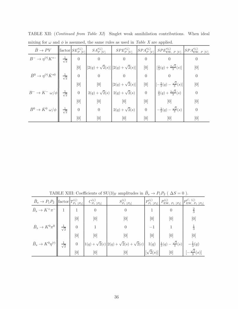
TABLE XII: (Continued from Table XI) Singlet weak annihilation contributions. When ideal
mixing for ω and φ is assumed, the same rules as used in Table X are applied.
B → PV factor SE′(ζ)P [V ] SA
′(ζ)P [V ] SPE
′(ζ)P [V ] SPA
′(ζ)P [V ] SPE
′(ζ)EW, P [V ] SPA
′(ζ)EW, P [V ]
B− → η(′)K∗− 1√2
0 0 0 0 0 0
[0] [2(q) +√2(s)] [2(q) +
√2(s)] [0] [ 43 (q) +
2√2
3 (s)] [0]
B0 → η(′)K∗0 1√2
0 0 0 0 0 0
[0] [0] [2(q) +√2(s)] [0] [− 2
3 (q)−√23 (s)] [0]
B− → K− ω/φ 1√2
0 2(q) +√2(s) 2(q) +
√2(s) 0 4
3 (q) +2√2
3 (s) 0
[0] [0] [0] [0] [0] [0]
B0 → K0 ω/φ 1√2
0 0 2(q) +√2(s) 0 − 2
3 (q)−√23 (s) 0
[0] [0] [0] [0] [0] [0]
TABLE XIII: Coefficients of SU(3)F amplitudes in Bs → P1P2 ( ∆S = 0 ).
Bs → P1P2 factor T(ζ)P1 [P2]
C(ζ)P1 [P2]
S(ζ)P1 [P2]
P(ζ)P1 [P2]
P(ζ)EW, P1 [P2]
PC, (ζ)EW, P1 [P2]
Bs → K+π− 1 1 0 0 1 0 23
[0] [0] [0] [0] [0] [0]
Bs → K0π0 1√2
0 1 0 −1 1 13
[0] [0] [0] [0] [0] [0]
Bs → K0η(′) 1√2
0 1(q) +√2(c) 2(q) +
√2(s) +
√2(c) 1(q) 1
3 (q)−√23 (s) −1
3(q)
[0] [0] [0] [√2(s)] [0] [−
√23 (s)]
36

TABLE XIV: (Continued from Table XIII) Weak annihilation contributions.
Bs → P1P2 factor E(ζ)P1 [P2]
A(ζ)P1 [P2]
PE(ζ)P1 [P2]
PA(ζ)P1 [P2]
PE(ζ)EW, P1 [P2]
PA(ζ)EW, P1 [P2]
Bs → K+π− 1 0 0 1 0 −13 0
[0] [0] [0] [0] [0] [0]
Bs → K0π0 1√2
0 0 −1 0 13 0
[0] [0] [0] [0] [0] [0]
Bs → K0η(′) 1√2
0 0 1(q) 0 − 13 (q) 0
[0] [0] [√2(s)] [0] [−
√23 (s)] [0]
TABLE XV: (Continued from Table XIV) Singlet weak annihilation contributions.
Bs → P1P2 factor SE(ζ)P1 [P2]
SA(ζ)P1 [P2]
SPE(ζ)P1 [P2]
SPA(ζ)P1 [P2]
SPE(ζ)EW, P1 [P2]
SPA(ζ)EW, P1 [P2]
Bs → K0η(′) 1√2
0 0 2(q) +√2(s) 0 − 2
3 (q)−√23 (s) 0
[0] [0] [0] [0] [0] [0]
TABLE XVI: Coefficients of SU(3)F amplitudes in Bs → P1P2 ( |∆S| = 1 ).
Bs → P1P2 factor T′(ζ)P1 [P2]
C′(ζ)P1 [P2]
S′(ζ)P1 [P2]
P′(ζ)P1 [P2]
P′(ζ)EW, P1 [P2]
PC′, (ζ)EW, P1 [P2]
Bs → π+π− 1 0 0 0 0 0 0
[0] [0] [0] [0] [0] [0]
Bs → π0π0 12 0 0 0 0 0 0
[0] [0] [0] [0] [0] [0]
Bs → K0K0 1 0 0 0 0 0 0
[0] [0] [0] [1] [0] [−13 ]
Bs → K−K+ 1 0 0 0 0 0 0
[1] [0] [0] [1] [0] [23 ]
Bs → π0η(′) 12 0 0 0 0 0 0
[0] [√2(s)] [0] [0] [
√2(s)] [0]
Bs → η(′)η(′) 12 0
√2(s, q) 2
√2(s, q) + 2(s, s) 2(s, s)
√23 (s, q) − 2
3 (s, s)
+2(s, c) +2(s, c) −23(s, s)
[0] [√2(s, q) [2
√2(s, q) + 2(s, s) [2(s, s)] [
√23 (s, q) [− 2
3 (s, s)]
+2(s, c)] +2(s, c)] −23(s, s)]
37

TABLE XVII: (Continued from Table XVI) Weak annihilation contributions.
Bs → P1P2 factor E′(ζ)P1 [P2]
A′(ζ)P1 [P2]
PE′(ζ)P1 [P2]
PA′(ζ)P1 [P2]
PE′(ζ)EW, P1 [P2]
PA′(ζ)EW, P1 [P2]
Bs → π+π− 1 0 0 0 1 0 −13
[1] [0] [0] [1] [0] [23 ]
Bs → π0π0 12 1 0 0 2 0 1
3
[1] [0] [0] [2] [0] [13 ]
Bs → K0K0 1 0 0 0 1 0 −13
[0] [0] [1] [1] [−13 ] [−1
3 ]
Bs → K−K+ 1 1 0 0 1 0 23
[0] [0] [1] [1] [−13 ] [−1
3 ]
Bs → π0η(′) 12 1(q) 0 0 0 0 1(q)
[1(q)] [0] [0] [0] [0] [1(q)]
Bs → η(′)η(′) 12 1(q, q) 0 2(s, s) 2(q, q) − 2
3 (s, s)13 (q, q)
+2(s, s) −23(s, s)
[1(q, q)] 0 [2(s, s)] [2(q, q) [− 23 (s, s)] [ 13 (q, q)
+2(s, s)] −23(s, s)]
TABLE XVIII: (Continued from Table XVII) Singlet weak annihilation contributions.
Bs → P1P2 factor SE′(ζ)P1 [P2]
SA′(ζ)P1 [P2]
SPE′(ζ)P1 [P2]
SPA′(ζ)P1 [P2]
SPE′(ζ)EW, P1 [P2]
SPA′(ζ)EW, P1 [P2]
Bs → π0η(′) 12
2(q) +√2(s) 0 0 0 0 2(q) +
√2(s)
[0] [0] [0] [0] [0] [0]
Bs → η(′)η(′) 12
2(q, q) 0 2√2(s, q) 4(q, q) + 2
√2(q, s) −
√2(s, q) 2
3(q, q) +
√2
3(q, s)
+√2(q, s) +2(s, s) +2
√2(s, q) + 2(s, s) − 2
3(s, s) −
√2(s, q)− 2
3(s, s)
[2(q, q) [0] [2√2(s, q) [4(q, q) + 2
√2(q, s) [−
√2(s, q) [ 2
3(q, q) +
√2
3(q, s)
+√2(q, s)] +2(s, s)] +2
√2(s, q) + 2(s, s)] − 2
3(s, s)] −
√2(s, q)− 2
3(s, s)]
38

TABLE XIX: Coefficients of SU(3)F amplitudes in Bs → PV ( ∆S = 0 ). When ideal mixing
for ω and φ is assumed, for Bs → K0ω (K0φ), set the coefficients of SU(3)F amplitudes with the
subscript K and the superscript ζ = s (q) to zero: i.e., for Bs → K0ω, S(s)K = P
(s)EW,K = 0, and for
Bs → K0φ, C(q)K = S
(q)K = P
(q)K = · · · = 0.
Bs → PV factor T(ζ)P [V ] C
(ζ)P [V ] S
(ζ)P [V ] P
(ζ)P [V ] P
(ζ)EW, P [V ] P
C, (ζ)EW, P [V ]
Bs → π−K∗+ 1 0 0 0 0 0 0
[1] [0] [0] [1] [0] [23 ]
Bs → π0K∗0 1√2
0 0 0 0 0 0
[0] [1] [0] [−1] [1] [13 ]
Bs → η(′)K∗0 1√2
0 0 0√2(s) 0 −
√23 (s)
[0] [1(q) +√2(c)] [2(q) +
√2(s) +
√2(c)] [1(q)] [ 13 (q)−
√23 (s)] [−1
3 (q)]
Bs → K+ρ− 1 1 0 0 1 0 23
[0] [0] [0] [0] [0] [0]
Bs → K0ρ0 1√2
0 1 0 −1 1 13
[0] [0] [0] [0] [0] [0]
Bs → K0 ω/φ 1√2
0 1(q) 2(q) +√2(s) 1(q) 1
3 (q)−√23 (s) −1
3(q)
[0] [0] [0] [√2(s)] [0] [−
√23 (s)]
39

TABLE XX: (Continued from Table XIX) Weak annihilation contributions. When ideal mixing
for ω and φ is assumed, the same rules as used in Table XIX are applied.
Bs → PV factor E(ζ)P [V ] A
(ζ)P [V ] PE
(ζ)P [V ] PA
(ζ)P [V ] PE
(ζ)EW, P [V ] PA
(ζ)EW, P [V ]
Bs → π−K∗+ 1 0 0 0 0 0 0
[0] [0] [1] [0] [−13 ] [0]
Bs → π0K∗0 1√2
0 0 0 0 0 0
[0] [0] [−1] [0] [13 ] [0]
Bs → η(′)K∗0 1√2
0 0√2(s) 0 −
√23 (s) 0
[0] [0] [1(q)] [0] [− 13 (q)] [0]
Bs → K+ρ− 1 0 0 1 0 −13 0
[0] [0] [0] [0] [0] [0]
Bs → K0ρ0 1√2
0 0 −1 0 13 0
[0] [0] [0] [0] [0] [0]
Bs → K0 ω/φ 1√2
0 0 1(q) 0 − 13 (q) 0
[0] [0] [√2(s)] [0] [−
√23 (s)] [0]
TABLE XXI: (Continued from Table XX) Singlet weak annihilation contributions. When ideal
mixing for ω and φ is assumed, the same rules as used in Table XIX are applied.
Bs → PV factor SE(ζ)P [V ] SA
(ζ)P [V ] SPE
(ζ)P [V ] SPA
(ζ)P [V ] SPE
(ζ)EW, P [V ] SPA
(ζ)EW, P [V ]
Bs → η(′)K∗0 1√2
0 0 0 0 0 0
[0] [0] [2(q) +√2(s)] [0] [− 2
3 (q)−√23 (s)] [0]
Bs → K0 ω/φ 1√2
0 0 2(q) +√2(s) 0 − 2
3 (q)−√23 (s) 0
[0] [0] [0] [0] [0] [0]
40

TABLE XXII: Coefficients of SU(3)F amplitudes in Bs → PV ( |∆S| = 1 ). When ideal mixing
for ω and φ is assumed, i) for Bs → π0ω (π0φ), set the coefficients of SU(3)F amplitudes with the
subscript π and the superscript ζ = s (q) to zero: i.e., for Bs → π0ω, SE′(s)π = SPA
′(s)EW,π = 0
[See Tabel XXIV.], and for Bs → π0φ, E′(q)π = PA
′(q)π = · · · = 0 [See Tabel XXIII.], and ii) for
Bs → η(′)ω [η(′)φ], set the coefficients of SU(3)F amplitudes with the superscript ζ = (s, s) or (q, s)
[(s, q) or (q, q)] to zero: i.e., for Bs → η(′)ω, C ′(q,s)ω = S
′(s,s)η(′)
= S′(q,s)ω = S
′(s,s)ω = · · · = 0, and for
Bs → η(′)φ, C ′(s,q)η(′)
= S′(s,q)η(′)
= P′(s,q)EW,η(′)
= 0.
Bs → PV factor T′(ζ)P [V ] C
′(ζ)P [V ] S
′(ζ)P [V ] P
′(ζ)P [V ] P
′(ζ)EW, P [V ] P
C′, (ζ)EW, P [V ]
Bs → π+ρ− 1 0 0 0 0 0 0
[0] [0] [0] [0] [0] [0]
Bs → π−ρ+ 1 0 0 0 0 0 0
[0] [0] [0] [0] [0] [0]
Bs → π0ρ0 12 0 0 0 0 0 0
[0] [0] [0] [0] [0] [0]
Bs → K0K∗0 1 0 0 0 0 0 0
[0] [0] [0] [1] [0] [−13 ]
Bs → K0K∗0 1 0 0 0 1 0 −13
[0] [0] [0] [0] [0] [0]
Bs → K−K∗+ 1 0 0 0 0 0 0
[1] [0] [0] [1] [0] [23 ]
Bs → K+K∗− 1 1 0 0 1 0 23
[0] [0] [0] [0] [0] [0]
Bs → π0 ω/φ 12 0 0 0 0 0 0
[0] [√2(s)] [0] [0] [
√2(s)] [0]
Bs → η(′)ρ0 12 0
√2(s) 0 0
√2(s) 0
[0] [0] [0] [0] [0] [0]
Bs → η(′) ω/φ 12 0
√2(s, q) 2
√2(s, q) + 2(s, s) 2(s, s)
√23 (s, q) − 2
3 (s, s)
−23(s, s)
[0] [√2(q, s) [2
√2(q, s) + 2(s, s) [2(s, s)] [
√23 (q, s) [− 2
3 (s, s)]
+2(c, s)] +2(c, s)] −23(s, s)]
41

TABLE XXIII: (Continued from Table XXII) Weak annihilation contributions. When ideal mixing
for ω and φ is assumed, the same rules as used in Table XXII are applied.
Bs → PV factor E′(ζ)P [V ] A
′(ζ)P [V ] PE
′(ζ)P [V ] PA
′(ζ)P [V ] PE
′(ζ)EW, P [V ] PA
′(ζ)EW, P [V ]
Bs → π+ρ− 1 0 0 0 1 0 −13
[1] [0] [0] [1] [0] [23 ]
Bs → π−ρ+ 1 1 0 0 1 0 23
[0] [0] [0] [1] [0] [−13 ]
Bs → π0ρ0 12 1 0 0 2 0 1
3
[1] [0] [0] [2] [0] [13 ]
Bs → K0K∗0 1 0 0 0 1 0 −13
[0] [0] [1] [1] [−13 ] [−1
3 ]
Bs → K0K∗0 1 0 0 1 1 −13 −1
3
[0] [0] [0] [1] [0] [−13 ]
Bs → K−K∗+ 1 1 0 0 1 0 23
[0] [0] [1] [1] [−13 ] [−1
3 ]
Bs → K+K∗− 1 0 0 1 1 −13 −1
3
[1] [0] [0] [1] [0] [23 ]
Bs → π0 ω/φ 12 1(q) 0 0 0 0 1(q)
[1(q)] [0] [0] [0] [0] [1(q)]
Bs → η(′)ρ0 12 1(q) 0 0 0 0 1(q)
[1(q)] [0] [0] [0] [0] [1(q)]
Bs → η(′) ω/φ 12 1(q, q) 0 2(s, s) 2(q, q) − 2
3 (s, s)13 (q, q)
+2(s, s) −23(s, s)
[1(q, q)] 0 [2(s, s)] [2(q, q) [− 23 (s, s)] [ 13 (q, q)
+2(s, s)] −23(s, s)]
42
TABLE XXIV: (Continued from Table XXIII) Singlet weak annihilation contributions. When ideal
mixing for ω and φ is assumed, the same rules as used in Table XXII are applied.
Bs → PV factor SE′(ζ)P [V ]
SA′(ζ)P [V ]
SPE′(ζ)P [V ]
SPA′(ζ)P [V ]
SPE′(ζ)EW, P [V ]
SPA′(ζ)EW, P [V ]
Bs → π0 ω/φ 12
2(q) +√2(s) 0 0 0 0 2(q) +
√2(s)
[0] [0] [0] [0] [0] [0]
Bs → η(′)ρ0 12
0 0 0 0 0 0
[2(q) +√2(s)] [0] [0] [0] [0] [2(q) +
√2(s)]
Bs → η(′) ω/φ 12
2(q, q) 0 2√2(s, q) 4(q, q) + 2
√2(q, s) − 2
√2
3(s, q) 2
3(q, q) +
√2
3(q, s)
+√2(q, s) +2(s, s) +2
√2(s, q) + 2(s, s) − 2
3(s, s) − 2
√2
3(s, q)− 2
3(s, s)
[2(q, q) [0] [2√2(q, s) [4(q, q) + 2
√2(s, q) [− 2
√2
3(q, s) [ 2
3(q, q) +
√2
3(s, q)
+√2(s, q)] +2(s, s)] +2
√2(s, q) + 2(s, s)] − 2
3(s, s)] − 2
√2
3(q, s)− 2
3(s, s)]
TABLE XXV: Numerical values of the SU(3)F amplitudes of Bu,d → P1P2 decays with ∆S = 0 and
|∆S| = 1 calculated in QCD factorization. The magnitude (in units of 10−9 GeV) and strong phase
(in degrees) of each SU(3)F amplitude are shown in order within the parenthesis : e.g., for the tree
amplitude TP ≡ |TP | ei(δP+θP ) with δP and θP being the strong and weak phases, respectively, its
magnitude and strong phase are shown as (|TP |, δP ).
∆S = 0 Numerical values |∆S| = 1 Numerical values
TP (24.52, 0.9◦) T ′P (6.90, 0.9◦)
CP (15.47, − 54.8◦) C ′P (4.48, − 56.6◦)
S(q)P (0.87, 159.1◦) S
′(q)P (4.11, 150.3◦)
S(s)P (0.89, 159.1◦) S
′(s)P (4.21, 150.3◦)
S(c)P (0.02, 159.1◦) S
′(c)P (0.09, 150.3◦)
PP (5.59, − 157.7◦) P ′P (34.25, − 157.4◦)
PEW, P (0.82, − 178.9◦) P ′EW, P (5.48, − 178.9◦)
PCEW, P (0.17, 163.9◦) PC′
EW, P (1.05, 163.1◦)
EP (1.96, 52.7◦) E′P (0.54, 52.9◦)
AP (0.61, − 127.3◦) A′P (0.17, − 127.1◦)
PEP (3.79, − 146.2◦) PE′P (21.19 , − 146.2◦)
PAP (0.61, − 127.3◦) PA′P (3.46, − 127.1◦)
PEEW, P (0.02, − 34.1◦) PE′EW, P (0.13, − 36.1◦)
PAEW, P (0.03, 52.7◦) PA′EW, P (0.15, 52.9◦)
43

TABLE XXVI: Same as Table XXV except for Bu,d → PV decays : e.g., for the tree amplitudes
(TP ; TV ) where TP,V ≡ |TP,V | ei(δP,V +θP,V ) with δP,V and θP,V being the strong and weak phases,
respectively, their magnitudes (in units of 10−9 GeV) and strong phases (in degrees) are shown as
(|TP |, δP ; |TV |, δV ).
∆S = 0 Numerical values |∆S| = 1 Numerical values
( TP ; TV ) ( 40.82, 0.8◦ ; 30.16, 0.8◦) ( T ′P
; T ′V
) ( 9.63, 0.8◦ ; 8.54, 0.8◦)
( CP ; CV ) ( 12.30, − 16.0◦ ; 11.84, − 51.7◦) ( C′P
; C′V
) ( 3.38, − 19.0◦ ; 2.79, − 55.4◦)
( S(q)P
; S(q)V
) ( 0.50, − 4.7◦ ; 0.79, 151.5◦) ( S′(q)P
; S′(q)V
) ( 2.75, − 5.6◦ ; 3.04, 134.2◦)
( S(s)P
; S(s)V
) ( 0.59, − 4.6◦ ; 0.81, 151.5◦) ( S′(s)P
; S′(s)V
) ( 3.22, − 5.5◦ ; 3.11, 134.2◦)
( S(c)P
; S(c)V
) ( − ; 0.02, 151.5◦) ( S′(c)P
; S′(c)V
) ( − ; 0.07, 134.2◦)
( PP ; PV ) ( 3.04, − 144.7◦ ; 3.12, 8.4◦) ( P ′P
; P ′V
) ( 17.99, − 144.4◦ ; 17.02, 7.9◦)
( PEW, P ; PEW, V ) ( 1.41, − 179.4◦ ; 1.01, − 178.9◦) ( P ′EW, P
; P ′EW, V
) ( 9.39, − 179.4◦ ; 6.00, − 178.9◦)
( PCEW, P
; PCEW, V
) ( 0.38, 165.0◦ ; 0.34, 164.7◦) ( PC′EW, P
; PC′EW, V
) ( 1.76, 165.1◦ ; 1.87, 160.6◦)
( EP ; EV ) ( 2.46, 70.1◦ ; 2.29, 38.9◦) ( E′P
; E′V
) ( 0.60, 69.4◦ ; 0.64, 39.2◦)
( AP ; AV ) ( 0.77, − 109.9◦ ; 0.72, − 141.1◦) ( A′P
; A′V
) ( 0.19, − 110.6◦ ; 0.20, − 140.8◦)
( PEP ; PEV ) ( 3.82, − 123.6◦ ; 3.83, 5.3◦) ( PE′P
; PE′V
) ( 19.83, − 124.2◦ ; 21.20, 5.0◦)
( PAP ; PAV ) ( 0.12, 70.1◦ ; 0.11, 38.9◦) ( PA′P
; PA′V
) ( 0.61, 69.4◦ ; 0.66, 39.2◦)
( PEEW, P ; PEEW, V ) ( 0.02, − 57.8◦ ; 0.14, − 157.3◦) ( PE′EW, P
; PE′EW, V
) ( 0.10, − 50.7◦ ; 0.77, − 157.0◦)
( PAEW, P ; PAEW, V ) ( 0.02, 70.1◦ ; 0.02, 38.9◦) ( PA′EW, P
; PA′EW, V
) ( 0.08, 69.4◦ ; 0.09, 39.2◦)
44

TABLE XXVII: Same as Table XXV except for Bs → P1P2 decays.
∆S = 0 Numerical values |∆S| = 1 Numerical values
TP (23.54, 0.9◦) T ′P (6.61, 0.8◦)
CP (19.57, − 51.6◦) C ′P (5.72, − 50.5◦)
S(q)P (1.31, 166.6◦) S
′(s,q)P (3.53, 162.5◦)
S(s)P (1.35, 166.6◦) S
′(s,s)P (3.62, 162.5◦)
S(c)P (0.03, 166.6◦) S
′(s,c)P (0.08, 162.5◦)
PP (5.64, − 158.1◦) P ′P (34.69, − 157.9◦)
PEW, P (0.78, − 178.9◦) P ′EW, P (4.46, − 178.8◦)
PCEW, P (0.25, 170.0◦) PC′
EW, P (1.58, 171.0◦)
EP (2.35, 51.2◦) E′P (0.65, 51.4◦)
AP (0.74, − 128.8◦) A′P (0.20, − 128.6◦)
PEP (4.31, − 149.1◦) PE′P (24.12, − 149.1◦)
PAP (0.74, − 128.8◦) PA′P (4.18, − 128.6◦)
PEEW, P (0.03, − 46.2◦) PE′EW, P (0.15, − 48.4◦)
PAEW, P (0.03, 51.2◦) PA′EW, P (0.18, 51.4◦)
TABLE XXVIII: Same as Table XXVI except for Bs → PV decays.
∆S = 0 Numerical values |∆S| = 1 Numerical values
( TP ; TV ) ( 39.33, 0.9◦ ; 30.59, 0.8◦) ( T ′P
; T ′V
) ( 9.28, 0.9◦ ; 8.60, 0.9◦)
( CP ; CV ) ( 15.49, − 12.5◦ ; 12.90, − 50.6◦) ( C′P
; C′V
) ( 3.59, − 13.0◦ ; 3.82, − 50.7◦)
( S(q)P
; S(q)V
) ( 0.64, − 3.6◦ ; 0.91, 155.3◦) ( S′(s,q)P
; S′(q,s)V
) ( 1.90, − 4.3◦ ; 4.56, 155.1◦)
( S(s)P
; S(s)V
) ( 0.76, − 3.6◦ ; 0.94, 155.3◦) ( S′(s,s)P
; S′(s,s)V
) ( 2.24, − 4.2◦ ; 4.68, 155.1◦)
( S(c)P
; S(c)V
) ( − ; 0.02, 155.3◦) ( S′(s,c)P
; S′(c,s)V
) ( − ; 0.10, 155.1◦)
( PP ; PV ) ( 2.82, − 142.7◦ ; 3.51, 7.7◦ ) ( P ′P
; P ′V
) ( 16.71, − 142.1◦ ; 19.83, 6.7◦)
( PEW, P ; PEW, V ) ( 1.38, − 179.4◦ ; 1.03, − 178.9◦) ( P ′EW, P
; P ′EW, V
) ( 6.61, − 179.4◦ ; 5.89, − 178.9◦)
( PCEW, P
; PCEW, V
) ( 0.48, 168.6◦ ; 0.36, 164.9◦) ( PC′EW, P
; PC′EW, V
) ( 2.30, 168.2◦ ; 2.10, 164.6◦)
( EP ; EV ) ( 3.24, 70.5◦ ; 2.44, 45.0◦) ( E′P
; E′V
) ( 0.79, 69.8◦ ; 0.68, 45.4◦)
( AP ; AV ) ( 1.01, − 109.5◦ ; 0.76, − 135.0◦) ( A′P
; A′V
) ( 0.25, − 110.2◦ ; 0.21, − 134.6◦)
( PEP ; PEV ) ( 4.87, − 123.4◦ ; 4.01, 16.3◦) ( PE′P
; PE′V
) ( 25.33, − 124.0◦ ; 22.29, 16.1◦)
( PAP ; PAV ) ( 0.16, 70.5◦ ; 0.12, 45.0◦) ( PA′P
; PA′V
) ( 0.81, 69.8◦ ; 0.70, 45.4◦)
( PEEW, P ; PEEW, V ) ( 0.03, − 63.1◦ ; 0.15, − 148.7◦) ( PE′EW, P
; PE′EW, V
) ( 0.13, − 56.1◦ ; 0.82, − 148.4◦)
( PAEW, P ; PAEW, V ) ( 0.02, 70.5◦ ; 0.02, 45.0◦) ( PA′EW, P
; PA′EW, V
) ( 0.11, 69.8◦ ; 0.09, 45.4◦)
45

[1] A. Ali and C. Greub, Phys. Rev. D 57, 2996 (1998).
[2] Y.H. Chen, H.Y. Cheng, B. Tseng and K.C. Yang, Phys. Rev. D 60, 094014 (1999).
[3] M. Beneke, G. Buchalla, M. Neubert and C.T. Sachrajda, Phys. Rev. Lett. 83, 1914 (1999);
Nucl. Phys. B 591, 313 (2000).
[4] Y.Y. Keum, H.-n. Li and A.I. Sanda, Phys. Rev. D 63, 054008 (2001).
[5] C.W. Bauer, D. Pirjol, I.Z. Rothstein and I.W. Stewart, Phys. Rev. D 70, 054015 (2004).
[6] L. L. Chau Wang, p. 419-431 in AIP Conference Proceedings 72 (1980), Weak Interactions as
Probes of Unification (edited by G.B. Collins, L.N. Chang and J.R. Ficenec), and p.1218-1232
in Proceedings of the 1980 Guangzhou Conference on Theoretical Particle Physics (Science
Press, Beijing, China, 1980, distributed by Van Nostrand Reinhold company); L. L. Chau,
Phys. Rep. 95, 1 (1983).
[7] L.L. Chau and H.Y. Cheng, Phys. Rev. Lett. 56, 1655 (1986).
[8] L.L. Chau and H.Y. Cheng, Phys. Rev. D 36, 137 (1987); Phys. Lett. B 222, 285 (1989).
[9] L.L. Chau, H.Y. Cheng, W. K. Sze, H. Yao, and B. Tseng, Phys. Rev. D 43, 2176-2192 (1991);
Phys. Rev. D 58, 019902(E) (1998).
[10] C. W. Chiang, M. Gronau, Z. Luo, J. L. Rosner and D. A. Suprun, Phys. Rev. D 69, 034001
(2004) [arXiv:hep-ph/0307395].
[11] C.W. Chiang, M. Gronau, J.L. Rosner and D. Suprun, Phys. Rev. D 70, 034020 (2004).
[12] C. W. Chiang, Y.F. Zhou, JHEP 0612, 027 (2006) [hep-ph/0609128].
[13] C. W. Chiang, Y. F. Zhou, JHEP 0903, 055 (2009) [arXiv:0809.0841 [hep-ph]].
[14] D. Zeppenfeld, Z. Phys. C 8, 77 (1981).
[15] M. Gronau, O. F. Hernandez, D. London, J. L. Rosner, Phys. Rev. D 50, 4529 (1994)
[hep-ph/9404283]; Phys. Rev. D 52, 6356 (1995) [hep-ph/9504326]; ibid., 6374 (1995)
[hep-ph/9504327]; A. S. Dighe, M. Gronau and J. L. Rosner, Phys. Lett. B 367, 357 (1996)
[Erratum-ibid. B 377, 325 (1996)] [arXiv:hep-ph/9509428]; Phys. Rev. D 57, 1783 (1998)
[hep-ph/9709223].
[16] S. Oh, Phys. Rev. D 60, 034006 (1999) [arXiv:hep-ph/9812530].
[17] N. G. Deshpande, X. -G. He, J. -Q. Shi, Phys. Rev. D 62, 034018 (2000) [hep-ph/0002260];
M. A. Dariescu, N. G. Deshpande, X. -G. He, G. Valencia, Phys. Lett. B 557, 60 (2003)
46

[hep-ph/0212333].
[18] X.Y. Li and S.F. Tuan, DESY Report No. 83-078 (unpublished); X.Y. Li, X.Q. Li, and P.
Wang, Nuovo Ciemento 100A, 693 (1988).
[19] L.L. Chau and H.Y. Cheng, Phys. Rev. D 39, 2788 (1989); L.L. Chau, H.Y. Cheng, and T.
Huang, Z. Phys. C 53, 413 (1992).
[20] M. Beneke, G. Buchalla, M. Neubert and C. T. Sachrajda, Phys. Rev. Lett. 83, 1914 (1999)
[arXiv:hep-ph/9905312]; Nucl. Phys. B 591, 313 (2000) [arXiv:hep-ph/0006124].
[21] M. Beneke and M. Neubert, Nucl. Phys. B 675, 333 (2003) [arXiv:hep-ph/0308039].
[22] M. Beneke, J. Rohrer and D. Yang, Nucl. Phys. B 774, 64 (2007) [arXiv:hep-ph/0612290].
[23] M. Wirbel, B. Stech, and M. Bauer, Z. Phys. C 29, 637 (1985); M. Bauer, B. Stech and
M. Wirbel, Z. Phys. C 34, 103 (1987).
[24] H. Y. Cheng and C. K. Chua, Phys. Rev. D 80, 114008 (2009) [arXiv:0909.5229 [hep-ph]];
ibid., 114026 (2009) [arXiv:0910.5237 [hep-ph]].
[25] P. Ball and R. Zwicky, Phys. Rev. D 71, 014015 (2005) [arXiv:hep-ph/0406232]; ibid., 014029
(2005) [arXiv:hep-ph/0412079].
[26] H. Y. Cheng, C. K. Chua and C. W. Hwang, Phys. Rev. D 69, 074025 (2004)
[arXiv:hep-ph/0310359].
[27] T. Feldmann, P. Kroll and B. Stech, Phys. Rev. D 58, 114006 (1998) [arXiv:hep-ph/9802409];
Phys. Lett. B 449, 339 (1999) [arXiv:hep-ph/9812269].
[28] P. Ball, G. W. Jones and R. Zwicky, Phys. Rev. D 75, 054004 (2007) [arXiv:hep-ph/0612081].
[29] H. Y. Cheng and C. K. Chua, Phys. Rev. D 80, 074031 (2009) [arXiv:0908.3506 [hep-ph]].
[30] A. S. Dighe, M. Gronau, J. L. Rosner, Phys. Rev. Lett. 79, 4333 (1997) [hep-ph/9707521];
C. W. Chiang and J. L. Rosner, Phys. Rev. D 65, 074035 (2002) [Erratum-ibid. D 68, 039902
(2003)] [arXiv:hep-ph/0112285]; H. K. Fu, X. G. He and Y. K. Hsiao, Phys. Rev. D 69, 074002
(2004) [arXiv:hep-ph/0304242]; C. W. Chiang, M. Gronau and J. L. Rosner, Phys. Rev. D
68, 074012 (2003) [arXiv:hep-ph/0306021].
[31] H.J. Lipkin, Phys. Lett. B 254, 247 (1991); Phys. Lett. B 433, 117 (1998).
[32] M. Beneke and M. Neubert, Nucl. Phys. B 651, 225 (2003) [arXiv:hep-ph/0210085].
47