Embed Size (px)
Citation preview
University of Wisconsin-Madison
Institute forResearch onPovertySpecial Report Series
AN EVALUATION OF VERTICALEQUITY .IN WISCONSIN'S~ERCENTAGE-OF-INCOMESTANDARDFOR CHILD SUPPORT
Robin A. Douthitt
May 1988
Special Report no. 47
An Evaluation of Vertical Equity in Wisconsin's
Percentage-of-Income Standard for Child Support
Robin A. DouthittSchool of Family Resources and Consumer Sciences
andInstitute for Research on PovertyUniversity of Wisconsin-Madison
May 1988
The research reported here was supported in part by a grant from theWisconsin Department of Health and Social Services to the Institute forResearch on Poverty. Any opinions expressed are solely those of theauthor.
Executive Summary
This report addresses the question of whether high-income families
allocate a smaller proportion of income to current consumption than do
low-income families. The question bears on the fairness of Wisconsin's
percentage-of-income standard for child support awards, since that stan
dardrequires larger payment amounts by high-income absent parents than
by their low-income counterparts. Canadian data on families in similar
economic circumstances to families in Wisconsin are used. A number of
measurement issues are involved in a study of this nature, in particular
use of gross versus net income and the choice of expenditure items to be
included in defining consumption.
The results of this study can be summarized as follows:
1. The share of total expenditures allocated by Canadian families to
current consumption is negatively related to both net and gross
income--the larger the income, the smaller is the expenditure
share allocated to current consumption.
2. The strength of the relationship between current consumption and
income depends on the choice among specific current consumption
measures. As more expenditures for durable goods are included in
measures of consumption, the smaller is the measured difference
between lower- and upper-income households in propensities to
consume out of gross income.
3. Only small differences are noted in the relationship of current
consumption share to net versus gross income.
4. The issue of whether implementation of a percentage-of-income
standard will result in payment by high-income absent parents of
an unfair share of child-rearing costs depends on the percentage
ii
levels established. Using Williams' estimates of child-rearing
costs as a benchmark, analysis indicates that application of the
Wisconsin percentage-of-income standard to establish child sup
port payments results in awards very close to actual child-
rea ring cos ts.
Several qualifications should be added:
1. Because Canadian families face a more progressive tax structure
than American families, these results may overstate the negative
relationship between consumption and income of U.S. families.
2. Methodological differences between this study and Espenshade's
study, on which Williams bases his. conclusions, will yield dif
ferences in results.
Implications of these results are as follows:
1. Further study using U.S. expenditure data is needed to determine
whether the negative relationship between income and share of
total expenditures allocated to current consumption can be repli
cated.
2. In Wisconsin the guiding principle in establishing child support
awards is that parents should share a percentage of their income
with their children whether or not they reside with them. This
approach has both conceptual and practical appeal. Conceptually,
it underscores the obligation of all parents, regardless of
income, to share resources with their children. Practically, it
provides flexible guidelines that are less costly to administer
through avoidance of methodological debates surrounding the esti
mation and updating of child-rearing costs. However, a benchmark
is needed to assess equity issues surrounding the percentages of
iii
income absent parents share with their children. Estimates of
child-rearing costs provide one comparative standard for eval
uating questions of "reasonableness" and "fairness." In this
report, child-rearing cost estimates are used to evaluate ver
tical equity issues surrounding implementation of Wisconsin's
child support award guidelines; e.g., the issue of how the
percentage-of-income standard affects higher- versus lower-income
absent parents in regard to support awards compared to awards
based directly on child-rearing cost estimates. The choice of
child-rearing costs as such a benchmark for impact evaluation
requires closer scrutiny of related measurement issues in future
work.
3. From a policy perspective, consideration should be given to the
extent to which expenditures on durables should be included in
child-rearing costs. This will have implications for whether
actual vertical inequities arise from application of Wisconsin's
percentage-of-income standard, since high-income families allo
cate a larger share of total expenditures to durables.
4. The current levels of gross income percentages established by
Wisconsin resul t in support awards that are comparable to the
levels of net income percentage guidelines suggested by
Espenshade/Williams. Thus, high-income absent parents under the
current gUidelines are paying support consistent with actual
child-rearing costs. However, the finding that a negative rela
tionship exists between consumption and income for Canadian fami
lies could imply that low-income absent parents are not paying
their full share of child-rearing costs.
An Evaluation of Vertical Equity in Wisconsin'sPercentage-of-Income Standard for Child Support
In 1982 Van der Gaag completed a comprehensive review of the econo-
mics literature on the costs of raising children. Conclusions drawn from
his study were used as the starting point for constructing the
percentage-of-income standard used in Wisconsin for establishing child
support awards. A conclusion of his study that "the share of income
devoted to children is roughly proportional up to very high income
levels" provided one justification for recommending that child support
awards be based on a constant percentage of the absent parent's gross
income (Van der Gaag, 1982).
Subsequently, this premise was challenged by Williams (1986), who
used findings by Espenshade (1984) to argue that the proportion of income
parents spend on their children declines as income increases. Espenshade
found that expenditures for children (1) increase with income and (2)
represent a constant proportion of families' current consumption.
However, Espenshade did not provide direct evidence regarding the rela-
tionship between consumption and income. Thus, Williams extrapolates by
augmenting Espenshade's findings and concludes that "As income increases,
total family current consumption declines as a proportion of net
(after-tax) income because non-current consumption increases with level
of household income •••• Moreover, family current consumption declines as
a proportion of gross (before-tax) income because of the progressive
federal and state income tax structure" (p. 24).
From these conclusions, Williams expresses concern that Wisconsin's
percentage-of-income standard child support formula is inequitable in
2
that high-income noncustodial parents would be required to pay a greater
proportion of net income in child support than their low-income counter
parts (p. 36). He recommends that the child support obligation of high
income noncustodial parents be calculated by applying a lower percentage
of gross income than that applied in determining the obligation of low
income parents.
In response to Williams' charges of vertical income inequities
arising from implementation of Wisconsin's percentage-of-income standard,
Garfinkel (1987) concedes that, although the weight of economic evidence
is not on Williams' side, the literature lacks any studies designed spe
cifically to examine the proportionality issue and calls for additional
study of the ques tion.
This paper is an initial study of the relationship between child
related expenditures and family income. For present purposes we accept
the Espenshade finding that expenditures for child-related goods and ser
vices represent a constant proportion of total current consumption by
families with children and focus on, first, disentangling taxes from
measures of consumption and income and, second, examining the rela
tionship between net income and current consumption of families with
children. We want to begin to answer the question, Do high-income fami
lies allocate a smaller proportion of net income to current consumption
than their low-income counterparts?
Finally, we question and examine implications of the implicit assump
tion of Williams that children only benefit from family expenditures for
3
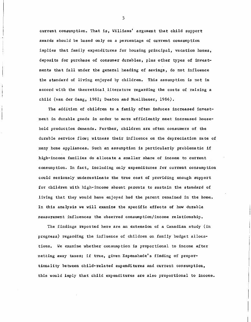
current consumption. That is, Williams' argument that child support
awards should be based only on a percentage of current consumption
implies that family expenditures for housing principal, vacation homes,
deposits for purchase of consumer durables, plus other types of invest
ments that fall under the general heading of savings, do not influence
the standard of living enjoyed by children. This assumption is not in
accord with the theoretical literature regarding the costs of raising a
child (van der Gaag, 1982; Deaton and Muellbauer, 1986).
The addition of children to a family often induces increased invest
ment in durable goods in order to more efficiently meet increased house
hold production demands. Further, children are often consumers of the
durable service flow; witness their influence on the depreciation rate of
many home appliances. Such an assumption is particularly problematic if
high-income families do allocate a smaller share of income to current
consumption. In fact, including only expenditures for current consumption
could seriously underestimate the true cost of providing enough support
for children with high-income absent parents to sustain the standard of
living that they would have enjoyed had the parent remained in the home.
In this analysis we will examine the specific effects of how durable
measurement influences the observed consumption/income relationship.
The findings reported here are an extension of a Canadian study (in
progress) regarding the influence of children on family budget alloca
tions. We examine whether consumption is proportional to income after
netting away taxes; if true, given Espenshade's finding of propor
tionality between child-related expenditures and current consumption,
this would imply that child expenditures are also proportional to income.
4
I. DATA AND THE MEASUREMENT OF TAXES
A major obstacle that has stood in the way of microeconomists' analy
sis of the consumption function has been identifying a data set that con
tains not only income, but also tax and consumption variables. In theory,
one would like to net away both consumption and income taxes paid by the
family prior to examining their relationship. Unfortunately, few data
sets include measures of all three.
The data employed in this study were collected as part of Statistics
Canada's 1982 Family Expenditure Survey. The survey contained questions
regarding income, expenditure, demographic and tax information from a
random sample of over 10,000 Canadian households. Unfortunately it was
primarily income taxes and not consumption taxes tha t were explicitly
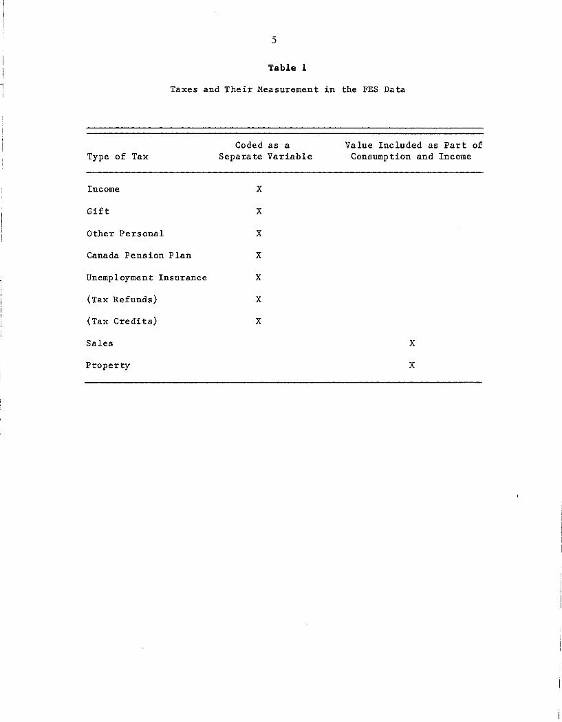
identified. Table 1 presents a list of taxes and how they were measured
in the FES.
Income, gift,and other personal taxes, net tax credits and refunds
are measured independently of either consumption or income. In addition,
measures of contributions to the Canada Pension Plan (the Canadian
equivalent to FICA deductions) and unemployment insurance are included in
the FES data. However, measures of both current consumption and income
are gross of sales and property taxes.
In order to minimize the effects of regional price differences, we
restricted our sample to families living in a single region of Canada.
Families living in the Western region (provinces of British Columbia,
Alberta, Saskatchewan and Manitoba) of Canada were chosen because of the
similarities between their economic circumstances (unemployment rates and
savings rates) and those of families living in the state of Wisconsin in
,
j
I1
5
Table 1
Taxes and Their Measurement in the FES Data
Type of Tax
Income
Gift
Other Personal
Canada Pension Plan
Unemployment Insurance
(Tax Refunds)
(Tax Credits)
Sales
Property
Coded as aSeparate Variable
x
x
x
x
x
x
x
Value Included as Part ofConsumption and Income
x
x
6
1982. A limitation in using this sample is that a family's specific pro
vince of residence cannot be established from the data. Families living
in the prairie provinces of Alberta, Saskatchewan, and Manitoba are
simply given the geographic code "prairies." Since provinces imposed
widely divergent sales tax policies,l regional aggregation precludes us
from imputing sales tax paid by each family.
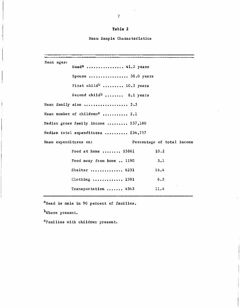
Our final sample consisted of 1630 husband-wife families (1) with
neither spouse older than 65 years of age, (2) not living on a farm, (3)
with all members present the entire year, and (4) whose income-tested
government assistance constituted no more than one-third of total income
in 1982. Mean sample characteristics are given in Table 2.
II. ANALYSIS OF THE INCOME-CONSUMPTION RELATIONSHIP
As noted in the introduc tion to this report, Williams regards both a
progressive tax system and the propensity for high-income families to
consume less of total income than their lower-income counterparts as
contributing to inequities arising from enforcement of the percentage-of
income standard. In this section we present an analysis of children's
influence on Canadian families' propensities to consume, net of the
effects of taxes.
Although it is arguable that Canadian families face a myriad of
market factors and have tastes that are different from those of similarly
situated families in the United States, many similarities in consumption
patterns in the two countries can be documented. Of special note are the
results of a pilot study to this project, where strikingly similar
7
Table 2
Mean Sample Characteristics
Mean ages:Heada •••••••••••••••• 41.2 years
Spouse ••••••••••••••••• 38.0 years
First childb ••••••••• 10.3 years
Second childb •••••••• 8.1 years
Mean family size ••••••••••••••••••• 3.3
Mean number of childrenc ••••••••••• 2.1
Median gross family income ••••••••• $37,180
Transportation ••••••• 4343
Food away from home •• 1190
Shelter •••••••••••••• 6231
Clo thing ••••••••••••• 2381
$3861 10.2
3.1
16.4
6.3
11.4
Percentage of total income
$34,757..........
........Food at home
Median total expenditures
Mean expenditures on:
aHead is male in 90 percent of families.
bWhere present.
cFamilies with children present.
8
results were found in replicating the analysis of 1972-73 expenditure
data2 for the northeastern United States, using 1982 Canadian Family
Expenditure Survey data (Fedyk, 1986).
Of perhaps more concern are the differences in tax policies of the
two countries. The tax incidence in Canada, particularly as it applies to
families with children, is more progressive than that faced by families
in the United States. 3 More specific differences will be enumerated as
we proceed to describe our analysis and apply its lessons to Wisconsin.
A. Methodology
In order to examine the relationship between family consumption and
income, we employ a multinomial logit budget share model (MLBAM) (from
Tyrrell, 1979) and twice estimate a simple consumption/saving system
using two different measures of income. First we estimate consumption as
a function of gross income--that is, the measure of income used is gross
of sales, property, income and other personal taxes. Next we reestimate
the system netting all taxes noted in Table 1 as having been coded
separately by Statistics Canada from gross income. Because of data
restrictions, measures of consumption and income in both estimates are
gross of property and sales taxes.
Contributions of this work include (1) the unique characteristics of
the chosen empirical model, (2) analysis of more recent expenditure data
than have previously been used, and (3) analysis of the model's sen
sitivity to specific consumption (savings) definitions.
Findings are based on results from an empirical model that incor
porates both continuous measures of adult equivalence and a flexible
9
functional form. In the study a revealed-preference approach using con
tinuous household size and structure variables is adopted. Although
revealed preference is a common approach for deriving equivalence
measures in the consumer demand 1iterature,4 few studies also incorporate
a continuous (versus stepwise discrete) approach to measure the effects
of family size and structure on spending behavior. 5 Friedman (1957)
first developed the concept of a continuous equivalence-scale measure.
Its strengths include continuity over size or age-range measures (i.e.,
scales do not "jump" between adjacent age categories) and fewer required
parameters for estimation. No studies in the consumer demand literature
whose purpose is to explicitly measure the costs of raising children have
used continuous scales.
The literature regarding the costs of raising children is replete
with examples of studies which incorporate econometric models that a
priori restrict estimated parameter values to be consistent with postu
lates of economic theory. For example, many expenditure allocation
models assume functions homogeneous of degree one in income and family
size (Prais and Houthakker, 1955). However, it can be demonstrated that
the assumption of homogeneity can generate nonsensical results when
applied to actual behavior and that homogeneity, coupled with an
equivalence-scale specifica tion, imp lies cons tant re turns to scale.
Numerous illustrations can be cited to refute the restriction that house
hold composition changes yield constant returns to scale. The purchase
of food in larger quantities sold at lower per unit prices and the reuse
of clothing are standard examples of economies of scale which often occur
upon the addition of a family member.
10
The present study incorporates a model which assures the theoretical
restrictions of adding-up while allowing for nonhomogeneous demand func
tions and economies of scale. Thus, the model provides an effective
balance between the concern for theoretical plausibility and the prac
tical need to explain variance in the data. 6
An additional contribution of this work is that it uses more recent
expenditure data than have previous studies. The data are taken from the
1982 Canadian Family Expenditure Survey (FES). Lazear and Michael (1980)
use the 1960-61 Survey of Consumer Expenditures, while Olson (1983),
Espenshade (1984), and van der Gaag and Smolensky (1982) all use the
1972-73 Consumer Expenditure Survey. Although Espenshade applies the cpr
to update expenditures to 1981 dollars, this approach can potentially
bias the results. For instance, if a change in relative prices occurs
over a period, causing families to substitute away from consumption of
goods that become relatively more costly, studies relying on dated expen
diture survey results will overstate (understate) the importance of com
modities whose prices have exceeded (fallen short of) the average
inflationary trend. This study's use of more recent expenditure data
enhances external validity of the empirical findings.
The final contribution of this study is its particular attention to
the model's sensitivity to definitions of consumption. As discussed in
the introduction, the treatment (measurement) of durable expenditures can
influence the consumption/income relationship. Most researchers in pre
vious studies simply adopt the collection agency's (Bureau of Labor
Statistics or Statistics Canada) definition of current consumption. The
problem with this approach concerns consistent treatment of durable
11
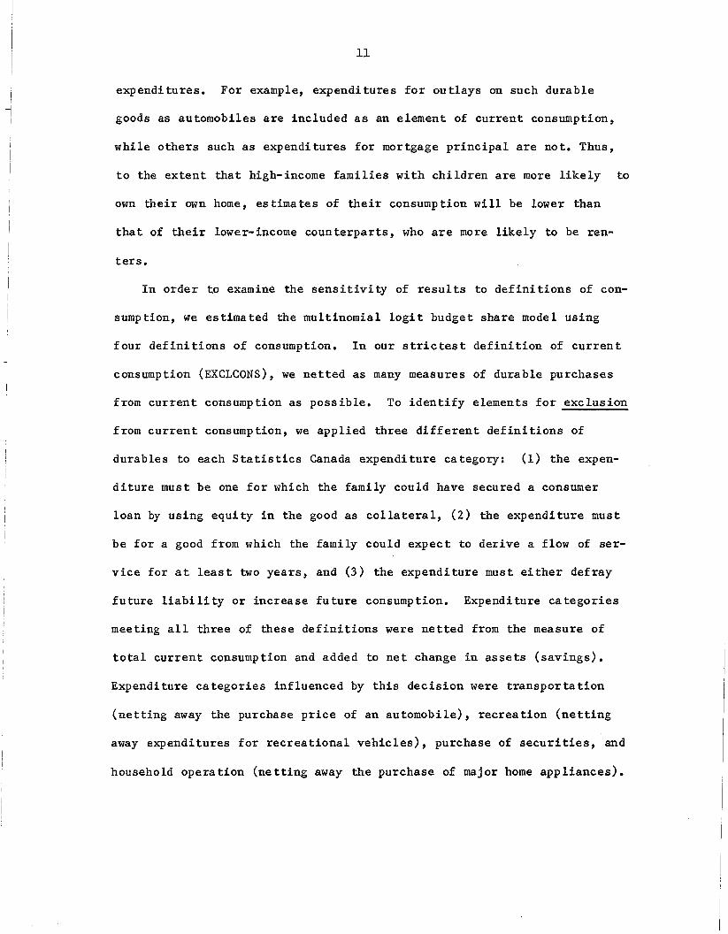
expenditures. For example, expenditures for outlays on such durable
goods as automobiles are included as an element of current consumption,
while others such as expenditures for mortgage principal are not. Thus,
to the extent that high-income families with children are more likely to
own their own home, estimates of their consumption will be lower than
that of their lower-income counterparts, who are more likely to be ren-
terse
In order to examine the sensitivity of results to definitions of con
sumption, we estimated the multinomial logit budget share model using
four definitions of consumption. In our strictest definition of current
consumption (EXCLCONS), we netted as many measures of durable purchases
from current consumption as possible. To identify elements for exclusion
from current consumption, we applied three different definitions of
durables to each Statistics Canada expenditure category: (1) the expen
diture must be one for which the family could have secured a consumer
loan by using equity in the good as collateral, (2) the expenditure must
be for a good from which the family could expect to derive a flow of ser
vice for at least two years, and (3) the expenditure must either defray
future liability or increase future consumption. Expenditure categories
meeting all three of these definitions were netted from the measure of
total current consumption and added to net change in assets (savings).
Expenditure categories influenced by this decision were transportation
(netting away the purchase price of an automobile), recreation (netting
away expenditures for recreational vehicles), purchase of securities, and
household operation (netting away the purchase of major home appliances).
12
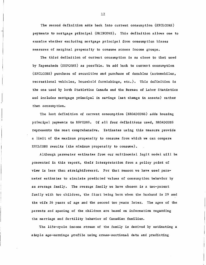
The second definition adds back into current consumption (EXCLCONS)
payments to mortgage principal (PRINCONS). This definition allows one to
examine whether excluding mortgage principal from consumption biases
measures of marginal propensity to consume across income groups.
The third definition of current consumption is as close to that used
by Espenshade (ESPCONS) as possible. We add back to current consumption
(EXCLCONS) purchase of securities and purchase of durables (automobiles,
recreational vehicles, household furnishings, etc.). This definition is
the one used by both Statistics Canada and the Bureau of Labor Statistics
and includes mortgage principal in savings (net change in assets) rather
than consumption.
The last definition of current consumption (BROADCONS) adds housing
principal payments to ESPCONS. Of all four definitions used, BROADCONS
represents the most comprehensive. Estimates using this measure provide
a limit of the maximum propensity to consume from which we can compare
EXCLCONS results (the minimum propensity to consume).
Although parameter estimates from our multinomial logit model will be
presented in this report, their interpretation from a policy point of
view is less than straightforward. For that reason we have used para
meter estimates to simulate predicted values of consumption behavior by
an average family. The average family we have chosen is a two-parent
family with two children, the first being born when the husband is 29 and
the wife 26 years of age and the second two years later. The ages of the
parents and spacing of the children are based on information regarding
the marriage and fertility behavior of Canadian families.
The life-cycle income stream of the family is derived by estimating a
simple age-earnings profile using cross-sectional data and predicting
13
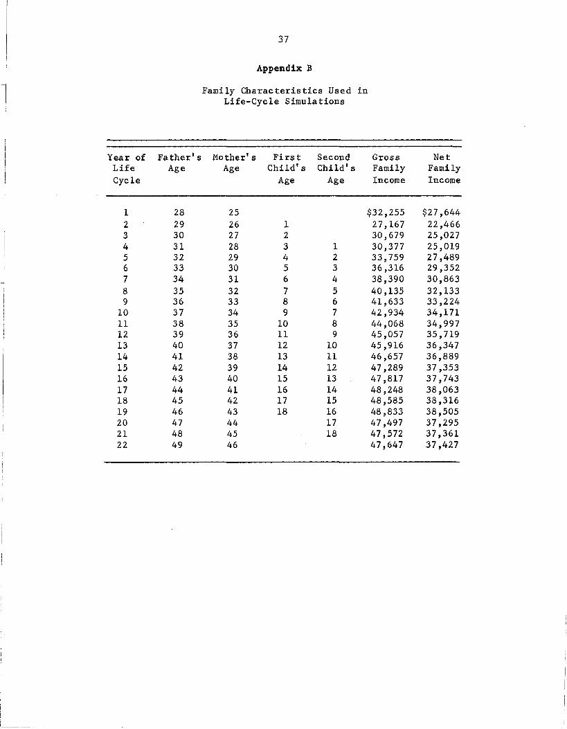
values from those parameter estimates. A table presenting the family
characteristics used in the simulations is presented in Appendix B.
B. Results
1. Evaluation of tax incidence
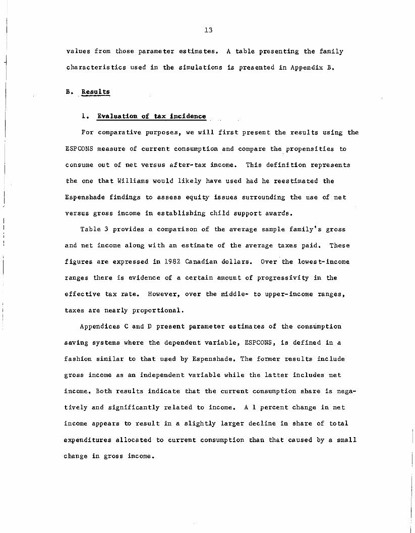
For comparative purposes, we will first present the results using the
ESPCONS measure of current consumption and compare the propensities to
consume out of net versus after-tax income. This definition represents
the one that Williams would likely have used had he reestimated the
Espenshade findings to assess equity issues surrounding the use of net
versus gross income in establishing child support awards.
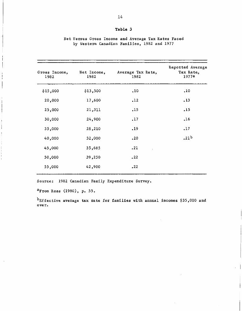
Table 3 provides a comparison of the average sample family's gross
and net income along with an estimate of the average taxes paid. These
figures are expressed in 1982 Canadian dollars. Over the lowest-income
ranges there is evidence of a certain amount of progressivity in the
effective tax rate. However, over the middle- to upper-income ranges,
taxes are nearly proportional.
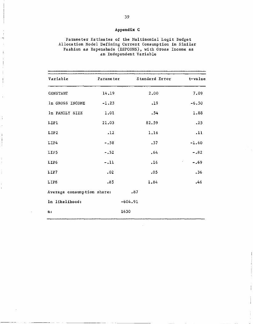
Appendices C and D present parameter estimates of the consumption
saving systems where the dependent variable, ESPCONS, is defined in a
fashion similar to that used by Espenshade. The former results include
gross income as an independent variable while the latter includes net
income. Both results indicate that the current consumption share is nega
tively and significantly related to income. A 1 percent change in net
income appears to result in a slightly larger decline in share of total
expenditures allocated to current consumption than that caused by a small
change in gross income.
14
Table 3
Net Versus Gross Income and Average Tax Rates Facedby Western Canadian Families, 1982 and 1977
Reported AverageGross Income, Net Income, Average Tax Rate, Tax Rate,
1982 1982 1982 1977a
$15,000 $13 ,500 .10 .10
20,000 17,600 .12 .13
25,000 21,311 .15 .15
30,000 24,900 .17 .16
35,000 28,210 .19 .17
40,000 32,000 .20 .21b
45,000 35,685 .21
50,000 39,250 .22
55,000 42,900 .22
Source: 1982 Canadian Family Expenditure Survey.
aFrom Ross (1980), p. 55.
bEffective average tax rate for families with annual incomes $35,000 andover.
15
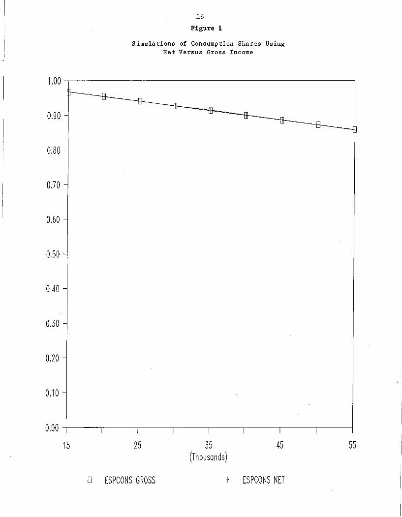
Figure 1 presents results of simulations using the respective para
meter estimates reported in Appendices C and D for our average family in
the year of the life cycle when the father is 41, the mother is 38, and
the two children are 11 and 13 years of age. Holding family charac
teristics constant, we repeat the simulation at various levels of income.
The two lines are virtually on top of one another, reflecting the negli
gible difference in consumption share when comparing net versus gross
income results at various income levels.
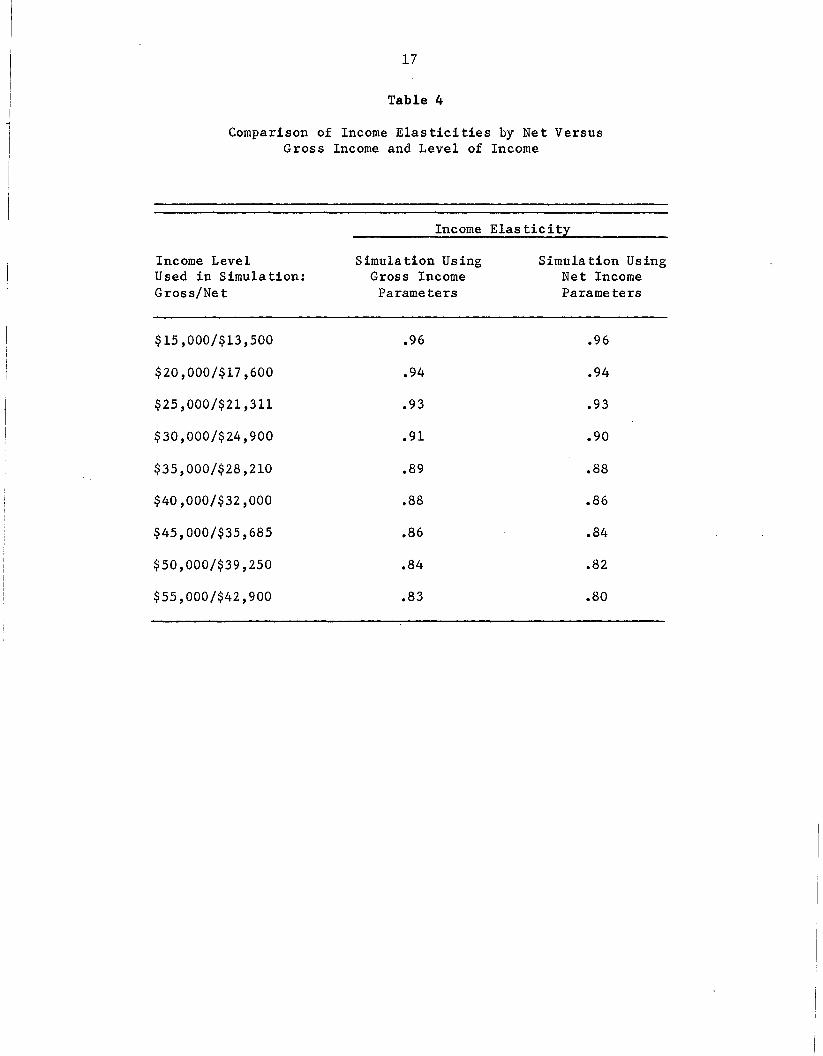
Table 4 presents income elasticity results using various levels of
net and gross income. Only at the uppermost levels of income are any dif
ferences apparent in the responsiveness of consumption to changes in net
versus gross income. A comparison of elasticities across income groups
confirms the result that the change in consumption share and the change
in income are negatively related, i.e., that as income increases by 1
percent, higher-income families are apt to respond by increasing consump
tion at a rate less than that of their lower-income counterparts,
ceteris paribus.
To summarize, our results indicate that (1) as a share of total
expenditures, there are no significant differences between families'
share allocation to current consumption out of net and gross income.
However, (2) there is a negative relationship between both gross and net
income in budget shares allocated to current consumption.
The first result seems to contradict findings reported by Williams
(p. 26) indicating an increasing difference between current consumption
out of gross and net income. 7 The second result tends to support
Williams' finding that higher-income families allocate a smaller share of
16
Figure 1
Simulations of Consumption Shares UsingNe t Versus Gross Income
554535(Thousands)
25
0.80
0.90
1.00 -,-----------------------------,
0.70
0.60
0.50
0.40
0.30
0.20
0.10
0.00 -+--__,---------.------,----,------r-----,-----,----------j
15
o ESPCONS GROSS + ESPCONS NET
17
Table 4
Comparison of Income Elasticities by Net VersusGross Income and Level of Income
Income Elasticity
Income Level Simulation Using Simula tion UsingUsed in Simulation: Gross Income Net IncomeGross/Net Parameters Parame ters
$15,000/$13,500 .96 .96
$20,000/$17,600 .94 .94
$25,000/$21,311 .93 .93
$30,000/$24,900 .91 .90
$35,000/$28,210 .89 .88
$40,000/$32,000 .88 .86
$45,000/$35,685 .86 .84
$50,000/$39,250 .84 .82
$55,000/$42,900 .83 .80
18
both net and gross income to current consumption. Yet, any conclusions
drawn from these results must be tempered by warnings regarding differen-
ces between this analysis and previous studies that may result from this
particular methodology and sample.
One methodological difference that may produce disparate findings
across studies is the interaction between variable measurement error and
the choice of model used in the analysis. In this study, as previously
mentioned, both consumption and income are gross of sales tax and pro-
perty tax. Espenshade's study suffers from similar measurement error.
However, the resulting bias will be influenced by the model chosen for
estimating the income-consumption relationship. For example, Espenshade
and Williams estimate family consumption as a linear function of hus-
bands' and wives' earnings and a product of each. In this study we esti-
mate consumption shares as a nonlinear function of total family income
from all sources. Thus
n > n > nedt'
where n is the true income elasticity with respect to current consumpt
tion as compared to those estimates bye, Espenshade, and d, Douthitt.
That is, the Espenshade results will yield an upward-biased income
elasticity as compared to both the actual and Douthitt elasticity esti-
mates. This implies that Espensh~de's results would overestimate the
extent to which the consumption behavior of high-income families would
respond to changes in income.
Potential differences in findings attributable to the sample are two-
fold. The first relates to the fact that the Canadian sample was drawn
"19
using different selection criteria from that used to draw the
Espenshade/Williams U.S. sample. Perhaps the major difference is the
fact that Canadian households were excluded if over one third of their
total family income was from income-tested government programs. The only
households deleted from Espenshade's study based on income were those
with incomplete reporting.
If families in the United States face a progressive incidence of
taxation, as claimed by Williams, the Canadian estimates of the rela
tionship between consumption and gross income will be understated. If,
however, U.S. policies, as reported by Pechman (1987), are slightly
regressive or at best proportional at the lower end of the income distri
bution, the fact that many of these households have been eliminated in
the Canadian study should introduce little or no bias with regard to the
true relationship for the upper quartiles of the population, but possibly
underestimate the relationship between consumption and gross income for
U.S. families at the lower end of the income distribution.
Second, different types of tax policies are applied to household
income in the American and Canadian samples, resulting in potential dif
ferences in tax incidence. One of the biggest differences between the
Canadian and U.S. federal tax policies is that mortgage interest is
deductible from taxable income in the United States, but not in Canada.
This may explain in part why analysis of Canadian tax incidence
(Gillespie, 1980) indicates that theirs is more progressive at the lower
end of the income distribution than is that of the United States.
However, given that we have restricted the Canadian sample to exclude
certain low-income families, this difference is not particularly germane
to our analysis.
20
The remaining bias depends on whether sales and property tax inci
dence (the two unaccounted-for tax policies) varies between the two
countries. There is little evidence to suggest these are significantly
different (as a percentage of current consumption) in the Canadian
regions analyzed and the state of Wisconsin in 1982.
2. Evaluation of current consumption measurement and its rela
tionship across income levels
As discussed in the introduction, the measurement of current consump
tion in the analysis of child-rearing costs is less straightforward than
some might like to believe. In this section we examine how sensitive the
relationship between income and current consumption across income levels
is to the measurement of the dependent variable.
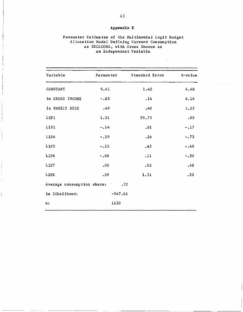
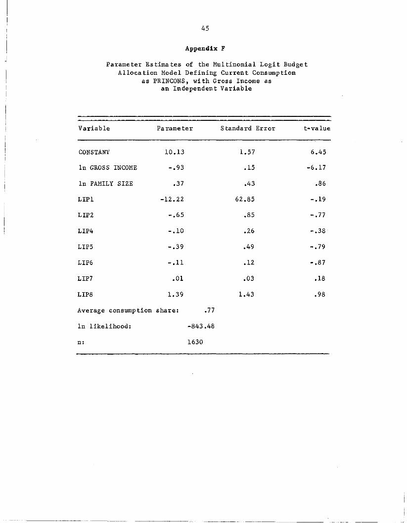
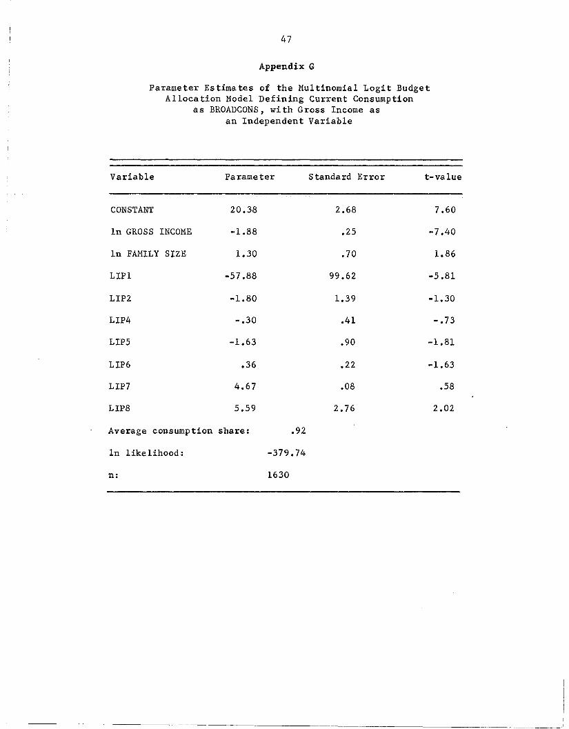
Appendices E, F, and G present parameters of the MLBAM model using
alternative definitions of current consumption. Since results appear
relatively invariant to specification of net or gross income as the inde
pendent variable, we will present only the results using gross income,
consistent with Wisconsin's specification of the income base.
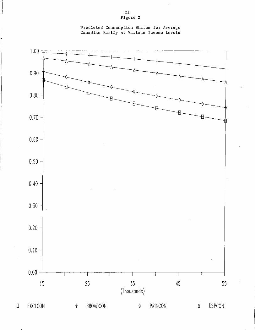
Definitionally, average consumption shares increase as the consump
tion share definition varies from EXCLCONS to BROADCONS. Further, the
larger the defined current consumption share, the less responsive it is
to changes in income. Figure 2 compares the predicted consumption shares
for our average family at various levels of income. This responsiveness
is reflected in the relative slope of each function. The slope of
BROADCONS is less steep than that of EXCLCONS.
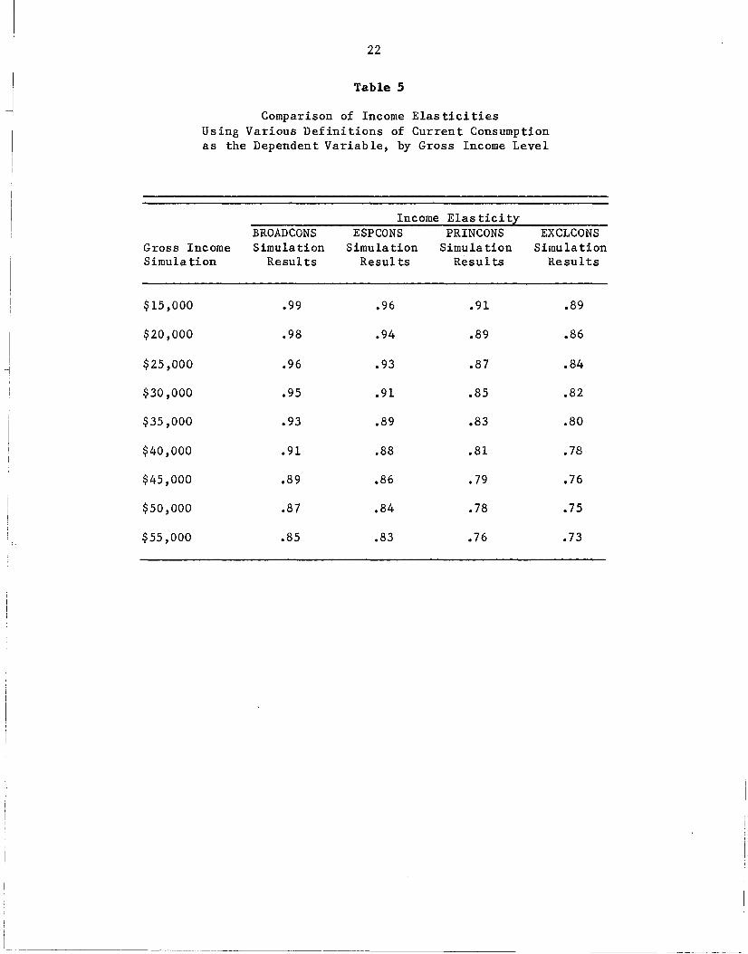
Table 5 presents a comparison of income elasticities at various
income levels for each definition of current consumption. The income
21Figure 2
Predicted Consumption Shares for AverageCanadian Family at Various Income Levels
1.00f~~~~:==:===::==:=====~l
554535(Thousands)
25
0,90
0.70
0,80
0,60
0,50
0.40
0.30
0,20
0,10
0,00 -1---,----,----,-------.-------.----------,-------.----1
15
D EXCLCON + BROADCON o PRINCON 8, ESPCON
22
Table 5
Comparison of Income ElasticitiesUsing Various Definitions of Current Consumptionas the Dependent Variable, by Gross Income Level
Income ElasticityBROADCONS ESPCONS PRINCONS EXCLCONS
Gross Income Simulation Simulation Simula tion SimulationSimula tion Results Resul ts Resul ts Results
$15,000 .99 .96 .91 .89
$20,000 .98 .94 .89 .86
$25,000 .96 .93 .87 .84
$30,000 .95 .91 .85 .82
$35,000 .93 .89 .83 .80
$40,000 .91 .88 .81 .78
$45,000 .89 .86 .79 .76
$50,000 .87 .84 .78 .75
$55,000 .85 .83 .76 .73
23
elasticity corresponding to the BROADCONS parameter estimate is nearly
unitary, implying that as gross income increases by 1 percent, the share
of current consumption will increase by the same amount.
The major implication of this analysis for evaluation of equity
issues surrounding implementation of the percentage-of-income standard
relates to the philosophical question of what expenditures should be con
sidered when assessing children's entitlement to their absent parent's
income. If the guiding principle is that children are entitled to a
level of support such that their standard of living does not vary from
what it would have been had the parents chosen to live together, then it
would be misguided to define consumption exclusive of all expenditures
for durables (EXCLCONS) that would have contributed to the child's stan
dard of living.
The implicit assumption in applying Espenshade's child-rearing cost
estimates to establish child support awards is that children are not
entitled to be compensated for housing expenditures applied to the prin
cipal of an owned home. This may be an equitable solution if, in addition
to a child support award, the absent parent is ordered to share mortgage
principal payments with the custodial parent residing in the matrimonial
home. In the absence of such an order, support orders based on
Espenshade's cost figures will tend to underestimate child-rearing costs,
particularly for those high-income families who are more likely to be
homeowners. Figure 2 and Appendix F support this conclusion by
demonstrating that smaller differences in shares of income allocated to
consumption across income groups are noted when durable goods purchases
are included in the consumption measure.
24
Thus, the definition of current consumption used to evaluate child
rearing costs has direct implications for assessing whether gross or net
income should be used as the income base in setting child support awards.
When expenditures for durable goods are included in consumption, there
appears to be less potential disparity in applying a single percentage
of-income standard across all income classes of absent parents.
III. DISCUSSION AND SUMMARY
The purpose of this analysis is to examine the relationship between
child-related expenditures and family income. The objective is to eva
luate whether Wisconsin's percentage-of-income standard to set child sup
port awards results in vertical income inequities between high- and
low-income absent parents--i.e., are high-income absent parents required
to pay a greater proportion of their net income in child support than
their low-income counterparts?
Analysis of Canadian expenditure data regarding family consumption
behavior provides mixed evidence regarding the equity issue. Like
Williams, we note that when the Espenshade definition of current consump
tion is used, families do tend to allocate a smaller share of their
expenditures to consumption as income increases. However, contrary to
Williams, we find no difference in allocations out of gross versus net
income.
Further analysis considered what, if any, influence a different defi
nition of current consumption from that used by Espenshade and others-
one including durable goods--had on the differences in observed
25
propensities to consume across income groups. Results indicate that this
definition does influence the relationship between consumption and
income. Specifically, if we include in our measure of consumption expen-
ditures for durable goods that contrib~te to child welfare and that are
more likely to be purchased by upper-income families, then smaller dif-
ferences across income groups are noted in the share of expenditures
a lloca ted to consump tion.
In the final analysis, however, what really matters is whether the
percentage-of-income standard set by the state of Wisconsin unfairly bur-
dens high-income absent parents. Contrary to Williams' assertion that
this standard will a priori be unfair to high-income parents, what is key
from an equity standpoint is the percentage standard level set by the
state. With knowledge of the tax rate faced by families at different
income levels, we could set Wisconsin's percentage-of-income standard so
that it yields a monthly child support payment equal to what it would
have been had net income been the income base. A simple formula for this
calcu la tion is
r * Y = (Y (l-t)) * rg n'
(1)
where r equals the percentage support applied to gross income, Y equalsg
gross income, t equals the tax rate faced by a family at that level of
gross income, and r equals the percentage support of net income appliedn
to the absent parent's income.
Since what is largely at issue in this whole evaluation is our inabi-
lity to accurately measure t, rigorous analysis of Wisconsin's
percentage-of-income standard cannot yet be accomplished. However, we do
26
have estimates of tax rates from the Canadian analysis and guidelines of
Williams (p. 26) regarding what both rand r should be for differentg n
income groups to make a "ballpark" assessment of the equity of
Wisconsin's percentage-of-income standard.
First, consider what the equivalent r should be if r equals 33.9g n
percent for an absent parent with two children and a net income of
$40,000 per year, as proposed by Williams (p. 26). Using the upper-
income tax rate of 22 percent, as found in the Canadian study, and
applying our formula (1), we see that an equivalent support payment based
on gross income would be 26 percent. The Wisconsin percentage-of-income
standard (r ) stands at 25 percent.g
If one believes that the weight of evidence regarding the rela-
tionship between consumption and income lies with the Williams study,
i.e., that there are significant differences across income categories in
propensi ties to consume out of gross income, then the implica tion of the
previous exercise is that the Wisconsin standard is a reasonable approxi-
mation of actual child-rearing costs. If, however, one believes that the
Williams evaluation of tax incidence is flawed in favor of the high-
income absent parent, then application of the Wisconsin standard yields
support levels below actual child-rearing costs for high-income absent
parents. Conversely, if one concurs with the Williams findings, then
low-income parents are not being ordered to make child support payments
sufficient to cover direct costs.
We can also assess the fairness of the percentage-of-income standard
by simply comparing it to the percentages of gross income that Williams
estimates as direct child-rearing costs (p. 26). Consistent with our
27
previous example of a parent whose net income is $40,000, we will now
consider support payments of a parent whose gross income is $50,000 (the
approximate income equivalent as calculated by both Williams in Table 5
and the author in Table 3). Williams finds that the parent of one, two,
or three children would allocate 17.6, 27.3 and 34.1 percent of gross
income, respectively, in support of their children. The Wisconsin stan
dard for one, two, and three children is 17, 25 and 29 percent, respec
tively. Thus, by Williams' own findings, the present percentage-of-income
standard levels do not appear unduly to burden the high-income absent
parent.
This evaluation is but a first step in examining the relationship of
consumption to income, and ultimately of child-rearing costs to income.
Some of its shortcomings can be addressed in part through analysis of
recent U.S. Bureau of Labor Statistics expenditure data. The next stage
of this evaluation is to replicate the Canadian study using these data.
29
Appendix A
METHODOLOGY
The "new home economics" (see Becker, 1981; Michael and Becker, 1973;
and Pollak and Wachter, 1975) serves as the theoretical framework on
which we build. We assume that households derive utility from the con-
sumption of home-produced commodities (Q), one of which is child ser-
vices. The inputs to the production process are time (t) and marke t goods
(x), which the household purchases with either unearned income (V) or
earnings (w) obtained from selling their labor (h) in the market.
Utility is maximized subject to time, income, and home production tech-
nology constraints. Input demand (expenditure) equations are derived by
solving the cost function dual problem for the household's expenditure
function.
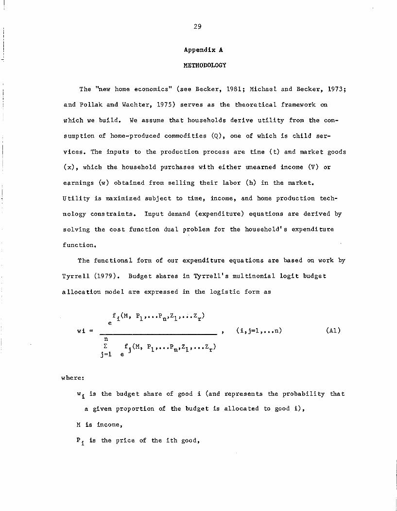
The functional form of our expenditure equations are based on work by
Tyrrell (1979). Budget shares in Tyrrell's multinomial logit budget
allocation model are expressed in the logistic form as
wi =
where:
nL f.(M, Pl' •••Pn ,Zl' ••• Zr)
j=l e J
(i,j=l, ••• n) (AI)
wi is the budge t share of good i (and represents the probabili ty that
a given proportion of the budge t is alloca ted to good i),
M is income,
Pi is the price of the ith good,
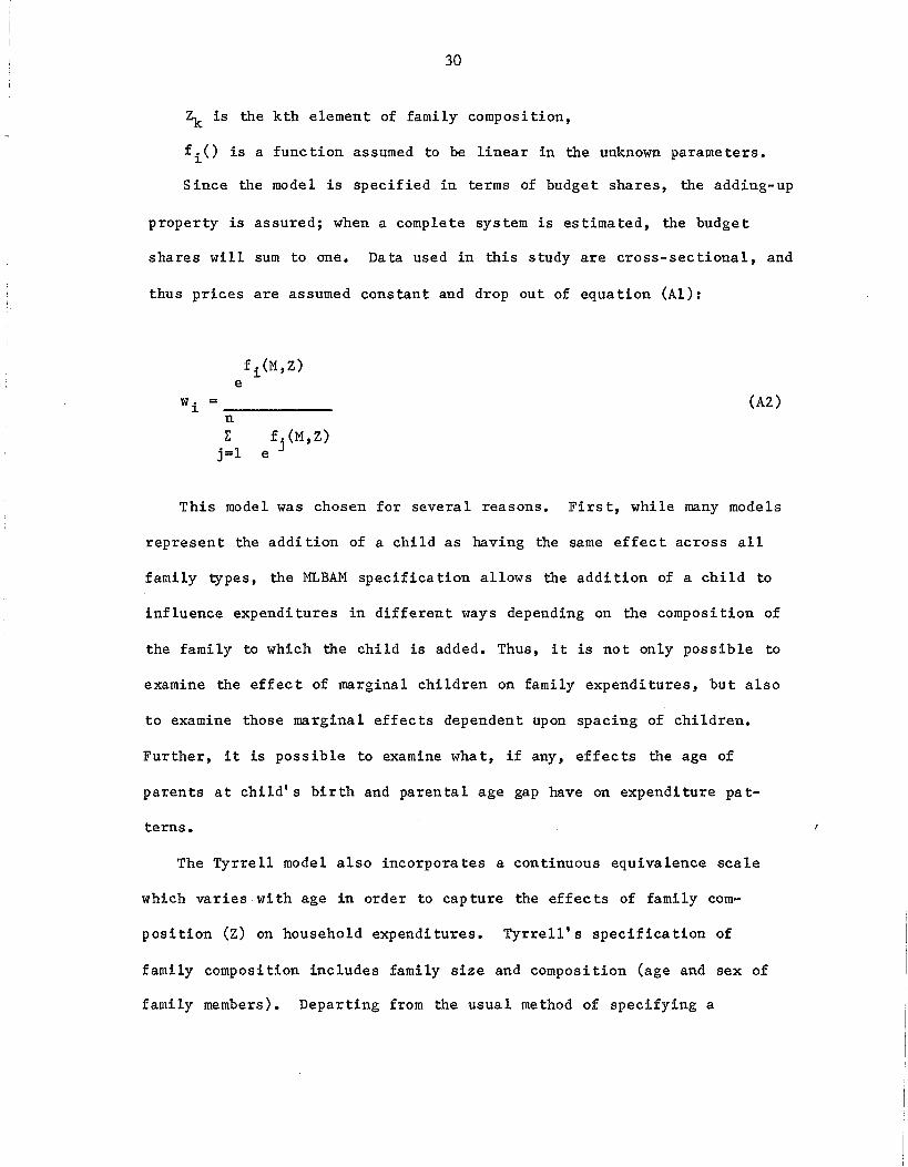
30
~ is the kth element of family composition,
f i () is a function assumed to be linear in the unknown parameters.
Since the model is specified in terms of budget shares, the adding-up
property is assured; when a complete system is estimated, the budget
shares will sum to one. Data used in this study are cross-sectional, and
thus prices are assumed constant and drop out of equation (Al):
wi = _n
(A2)
This model was chosen for several reasons. First, while many models
represent the addition of a child as having the same effect across all
family types, the MLBAM specification allows the addition of a child to
influence expenditures in different ways depending on the composition of
the family to which the child is added. Thus, it is not only possible to
examine the effect of marginal children on family expenditures, but also
to examine those marginal effects dependent upon spacing of children.
Further, it is possible to examine what, if any, effects the age of
parents at child's birth and parental age gap have on expenditure pat-
terns.
The Tyrrell model also incorporates a continuous equivalence scale
which varies with age in order to capture the effects of family com-
position (2) on household expenditures. Tyrrell's specification of
family composition includes family size and composition (age and sex of
family members). Departing from the usual method of specifying a
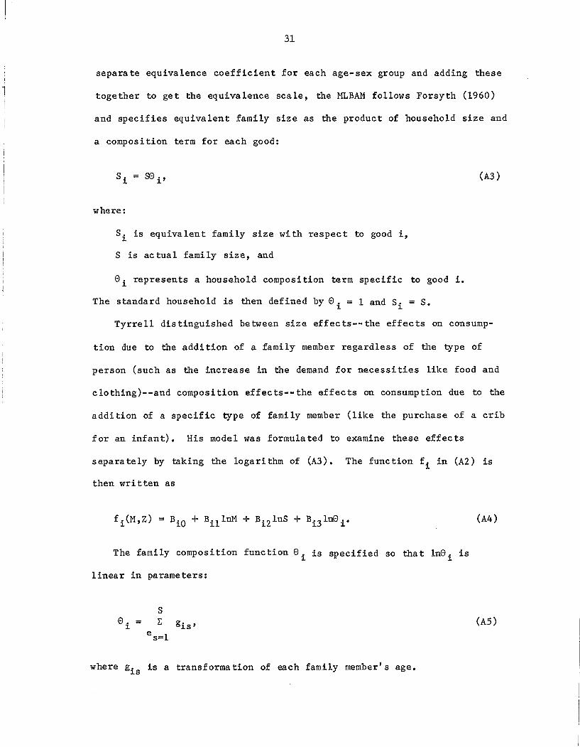
31
separate equivalence coefficient for each age-sex group and adding these
together to get the equivalence scale, the MLBAM follows Forsyth (1960)
and specifies equivalent family size as the product of household size and
a composition term for each good:
(A3)
where:
Si is equivalent family size with respect to good i,
S is ac tual family size, and
Gi represents a household composi tion term specific to good i.
The standard household is then defined by G i = 1 and Si = S.
Tyrrell distinguished between size effects--the effects on consump-
tion due to the addi Hon of a family member regardless of the type of
person (such as the increase in the demand for necessities like food and
clothing)--and composition effects--the effects on consumption due to the
addition of a specific type of family member (like the purchase of a crib
for an infant). His model was formulated to examine these effects
s epa ra te ly by taking the logari thm of (A3). The func Hon f i in (A2) is
then written as
(A4)
The family compos i Hon func Hon G i is specified so tha t InG i is
linear in parameters:
SG. = L
~
es=l
where g. is a transformation of each family member's age.~s
(AS)
32
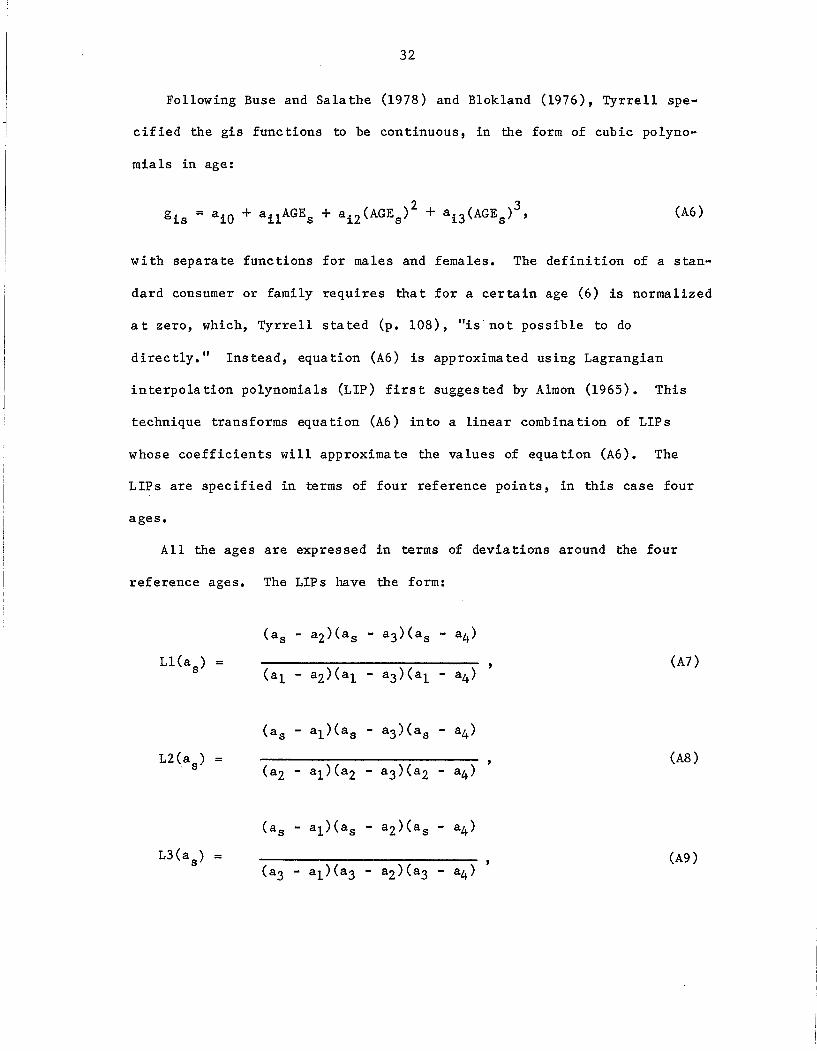
Following Buse and Salathe (1978) and Blokland (1976), Tyrrell spe-
cified the gis functions to be continuous, in the form of cubic polyno-
mials in age:
(A6)
with separate functions for males and females. The definition of a stan-
dard consumer or family requires that for a certain age (6) is normalized
a t zero, which, Tyrrell stated (p. 108), "is· not possible to do
directly." Instead, equation (A6) is approximated using Lagrangian
interpolation polynomials (LIP) first suggested by Almon (1965). This
technique transforms equation (A6) into a linear combination of LIPs
whose coefficients will approximate the values of equation (A6). The
LIPs are specified in terms of four reference points, in this case four
ages.
All the ages are expressed in terms of deviations around the four
reference ages. The LIPs have the form:
(An
(A8)
(A9)
33
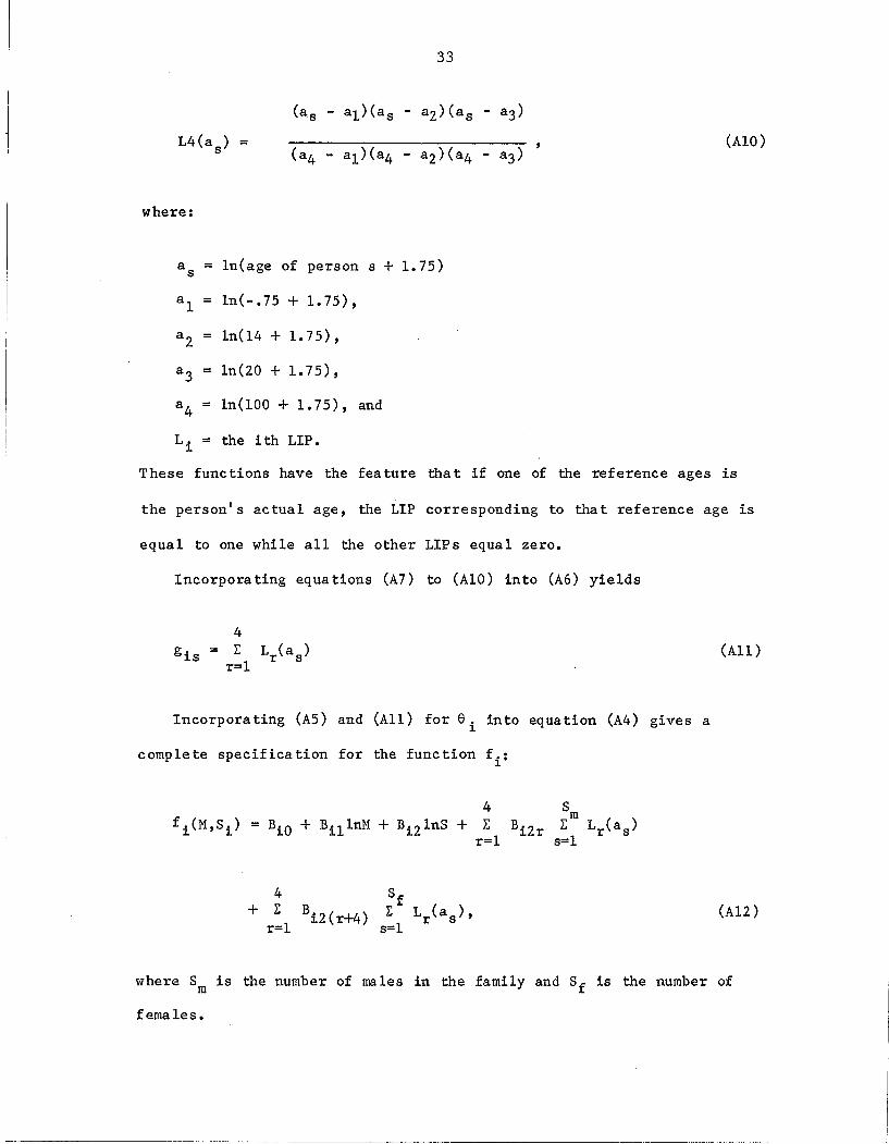
(A10)
where:
as = 1n(age of person s + 1.75)
a l = 1n(-.75 + 1.75),
a Z 1n(14 + 1.75),
a 3 = 1n(ZO + 1.75),
a 4 = In(100 + 1.75), and
L i = the ith LIP.
These func tions have the fea ture tha t if one of the reference ages is
the person's actual age, the LIP corresponding to that reference age is
equal to one while all the other LIPs equal zero.
Incorporating equations (A7) to (A10) into (A6) yields
Incorpora ting (A5) and (All) for e. in to eq ua tion (A4 ) gives a1.
complete specification for the function f i :
(All)
f.(M,S.)1. 1.
(A1Z)
where Sm is the number of males in the family and Sf is the number of
females.
34
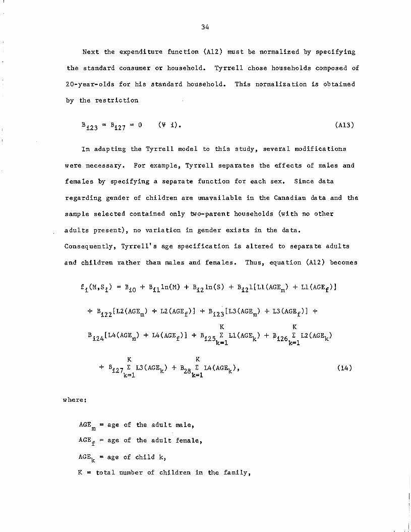
Next the expenditure function (A1Z) must be normalized by specifying
the standard consumer or household. Tyrrell chose households composed of
ZO-year-01ds for his standard household. This normalization is obtained
by the restriction
(v i). (A13)
In adapting the Tyrrell model to this study, several modifications
were necessary. For example, Tyrrell separates the effects of males and
females by specifying a separate function for each sex. Since data
regarding gender of children are unavailable in the Canadian data and the
sample selected contained only two-parent households (wi th no other
adults present), no variation in gender exists in the data.
Consequently, Tyrrell's age specification is altered to separate adults
and children rather than males and females. Thus, equation (A1Z) becomes
+ BiZZ[LZ(AGEm) + LZ(AGE f )] + BiZ3 [L3(AGEm) + L3(AGE f )] +
K KBiZ4 [L4(AGEm) + L4(AGEf )] + BiZ5k:1L1(AGEk) + BiZ6k:1LZ(AGEk)
where:
K K+ BiZ7 ~ L3(AGEk ) + BZ8 ~ L4(AGEk ),
k=l k=l(14)
AGE = age of the adult male,m
AGEf = age of the adult female,
AGEk = age of child k,
K = total number of children in the family,
35
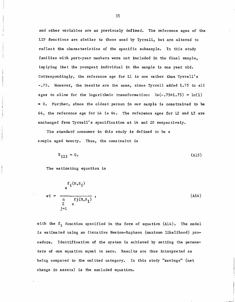
and other variables are as previously defined. The reference ages of the
LIP functions are similar to those used by Tyrrell, but are altered to
reflect the characteristics of the specific subsample. In this study
families with part-year members were not included in the final sample,
implying that the youngest individual in the sample is one year old.
Correspondingly, the reference age for Ll is one rather than Tyrrell's
-.75. However, the results are the same, since Tyrrell added 1.75 to all
ages to allow for the logarithmic transformation: In(-.75+1.75) = In(l)
= O. Further, since the oldest person in our sample is constrained to be
64, the reference age for 14 is 64. The reference ages for L2 and L3 are
unchanged from Tyrrell's specification at 14 and 20 respectively.
The standard consumer in this study is defined to be a
couple aged twenty. Thus, the constraint is
Bi23 = O. (A15)
The estimating equation is
wi =nL
j=l
(A16)
with the f i function specified in the form of equation (A14). The model
is estimated using an iterative Newton-Raphson (maximum likelihood) pro-
cedure. Identification of the system is achieved by setting the parame-
ters of one equa tion equal to zero. Resul ts are thus interpreted as
being compared to the omitted category. In this study "savings" (net
change in assets) is the excluded equation.
37
Appendix B
Family Characteristics Used inLife-Cycle Simulations
Year of Father's Mother's First Second Gross NetLife Age Age Child's Child's Family FamilyCycle Age Age Income Income
1 28 25 $32,255 $27,6442 29 26 1 27,167 22,4663 30 27 2 30,679 25,0274 31 28 3 1 30,377 25,0195 32 29 4 2 33,759 27,4896 33 30 5 3 36,316 29,3527 34 31 6 4 38,390 30,8638 35 32 7 5 40,135 32,1339 36 33 8 6 41,633 33,224
10 37 34 9 7 42,934 34,17111 38 35 10 8 44,068 34,99712 39 36 11 9 45,057 35,71913 40 37 12 10 45,916 36,34714 41 38 13 11 46,657 36,88915 42 39 14 12 47,289 37,35316 43 40 15 13 47,817 37,74317 44 41 16 14 48,248 38,06318 45 42 17 15 48,585 38,31619 46 43 18 16 48,833 38,50520 47 44 17 47,497 37,29521 48 45 18 47,572 37,36122 49 46 47,647 37,427
39
Appendix C
Parameter Estimates of the Multinomial Logit BudgetAllocation Model Defining Current Consumption in Similar
Fashion as Espenshade (ESPCONS), with Gross Income asan Independent Variable
Variable Parame ter Standard Error t-value
CONSTANT 14.19 2.00 7.09
1n GROSS INCOME -1.23 .19 -6.50
In FAMILY SIZE 1.01 .54 1.88
LIPl 21.03 82.59 .25
LIP2 .12 1.16 .11
LIP4 -.58 .37 -1.60
LIP5 -.52 .64 -.82
LIP6 - .11 .16 -.69
LIP7 .02 .05 .36
LIP8 .85 1.84 .46
Average consump tion share: .87
In like lihood: -604.91
n: 1630

41
Appendix D
Parameter Estimates of the Multinomial Logit BudgetAllocation Model Defining Current Consumption in Similar
Fashion as Espenshade (ESPCONS), with Net Income asan Independent Variable
Variable Parameter Standard Error t-value
CONSTANT 15.61 2.13 7.33
In NET INCOME -1.39 .20 -6.77
In FAMILY SIZE 1.09 .54 2.03
LIPI 20.85 82 .. 66 .25
LIP2 .13 1.16 11.31
LIP4 -.59 .37 -1.61
LIP5 -.56 .64 -.88
LIP6 -.12 .16 -.76
LIP7 .02 .05 .42
LIP8 .97 1.85 .52
Average cons'ump tion share: .87
In like lihood: -603.12
n: 1630
43
Appendix E
Parameter Estimates of the Multinomial Logit BudgetAllocation Model Defining Current Consumption
as EXCLCONS, with Gross Income asan Independent Variable
Variable Parameter Standard Error t-va1ue
CONSTANT 9.41 1.45 6.48
In GROSS INCOME -.85 .14 6.16
In FAMILY SIZE .49 .40 1.23
LIPI l.51 59.75 .03
LIP2 -.14 .81 -.17
LIP4 -.19 .26 -.75
LIP5 -.22 .45 -.49
LIP6 -.06 .11 -.50
LIP7 .00 .02 .48
LIP8 .39 1.31 .30
Average consump tion share: .72
In like lihood: -947.61
n: 1630
45
Appendix F
Parame ter Es tima tes of the Mul tinomial Logi t Budge tAllocation Model Defining Current Consumption
as PRINCONS, with Gross Income asan Independent Variable
Variable Parameter Standard Error t-value
CONSTANT 10.13 1.57 6.45
In GROSS INCOME -.93 .15 -6.17
In FAMILY SIZE .37 .43 .86
LIPI -12.22 62.85 -.19
LIP2 -.65 .85 -.77
LIP4 -.10 .26 -.38
LIP5 -.39 .49 -.79
LIP6 - .11 .12 -.87
LIP7 .01 .03 .18
LIP8 1.39 1.43 .98
Average consump tion share: .77
In likelihood: -843.48
n: 1630
47
Appendix G
Parameter Estimates of the Multinomial Logit BudgetAllocation Model Defining Current Consumption
as BROADCONS, with Gross Income asan Independent Variable
Variable Parameter Standa rd Error t-value
CONSTANT 20.38 2.68 7.60
In GROSS INCOME -1.88 .25 -7.40
In FAMILY SIZE 1.30 .70 1.86
LIPI -57.88 99.62 -5.81
LIP2 -1.80 1.39 -1.30
LIP4 -.30 .41 -.73
LIPS -1.63 .90 -1.81
LIP6 .36 .22 -1.63
LIP7 4.67 .08 .58
LIP8 5.59 2.76 2.02
Average consump tion share: .92
In like lihood : -379.74
n: 1630
49
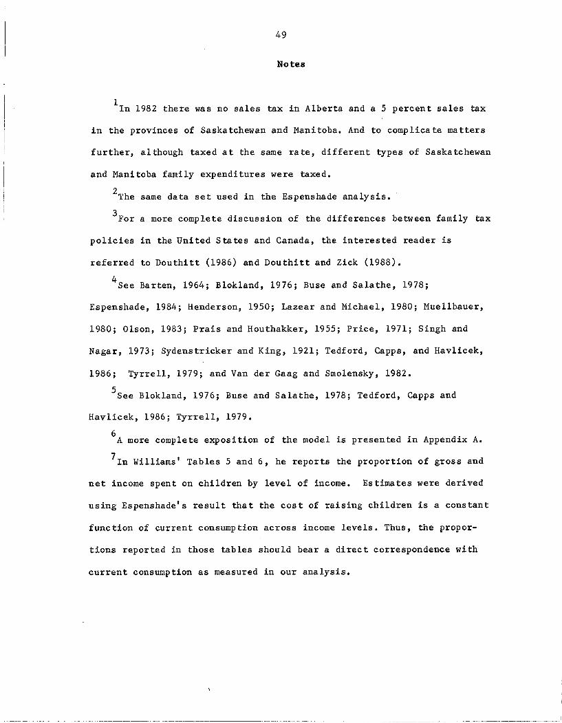
Notes
lIn 1982 there was no sales tax in Alberta and a 5 percent sales tax
in the provinces of Saskatchewan and Manitoba. And to complicate matters
further, although taxed at the same rate, different types of Saskatchewan
and Manitoba family expenditures were taxed.
2The same data set used in the Espenshade analysis.
3For a more complete discussion of the differences between family tax
policies in the United States and Canada, the interested reader is
referred to Douthitt (1986) and Douthitt and Zick (1988).
4 See Barten, 1964; Blokland, 1976; Buse and Salathe, 1978;
Espenshade, 1984; Henderson, 1950; Lazear and Michael, 1980; Muellbauer,
1980; Olson, 1983; Prais and Houthakker, 1955; Price, 1971; Singh and
Nagar, 1973; Sydenstricker and King, 1921; Tedford, Capps, and Havlicek,
1986; Tyrrell, 1979; and Van der Gaag and Smolensky, 1982.
5See Blokland, 1976; Buse and Salathe, 1978; Tedford, Capps and
Havlicek, 1986; Tyrrell, 1979.
6A more complete exposition of the model is presented in Appendix A.
7In Williams' Tables 5 and 6, he reports the proportion of gross and
net income spent on children by level of income. Estimates were derived
using Espenshade's result that the cost of raising children is a constant
function of current consumption across income levels. Thus, the propor
tions reported in those tables should bear a direct correspondence with
current consumption as measured in our analysis.
51
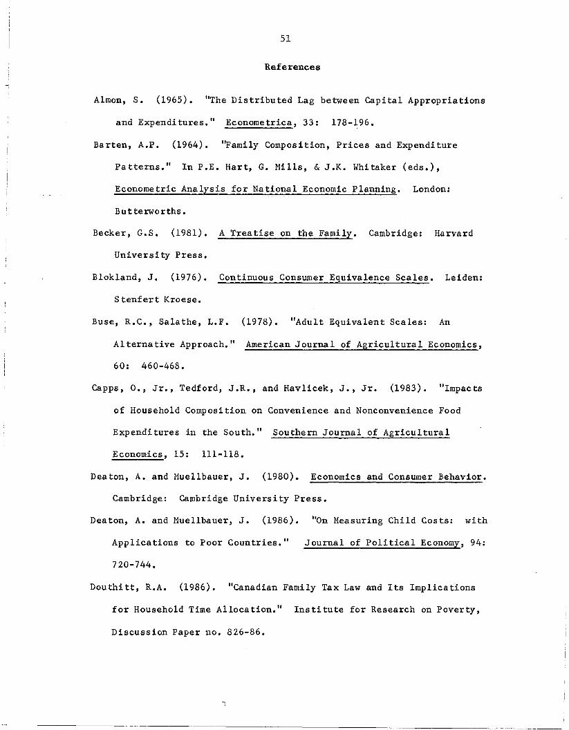
References
Almon, S. (1965). liThe Distributed Lag between Capital Appropriations
and Expenditures." Econometrica, 33: 178-196.
Barten, A.P. (1964). "Family Composition, Prices and Expenditure
Patterns." InP.E. Hart, G. Mills, &J.K. Whitaker (eds.),
Econometric Analysis for National Economic Planning. London:
Bu t terworths.
Becker, G.S. (1981). A Treatise on the Family. Cambridge: Harvard
University Press.
Blokland, J. (1976). Continuous Consumer Equivalence Scales. Leiden:
S tenfert Kroese.
Buse, R.C., Salathe, L.F. (1978). "Adult Equivalent Scales: An
Alternative Approach. II American Journal of Agricultural Economics,
60: 460-468.
Capps, 0., Jr., Tedford, J.R., and Havlicek, J., Jr. (1983). "Impacts
of Household Composition on Convenience and Nonconvenience Food
Expenditures in the South. II Southern Journal of Agricultural
Economics, 15: 111-118.
Deaton, A. and Muellbauer, J. (1980). Economics and Consumer Behavior.
Cambridge: Cambridge University Press.
Deaton, A. and Muellbauer, J. (1986). liOn Measuring Child Costs: with
Applications to Poor Countries." Journal of Political Economy, 94:
720-744.
Dou thi tt, R.A. (1986). "Canadian Family Tax Law and Its Implications
for Household Time Allocation." Institute for Research on Poverty,
Discussion Paper no. 826-86.
52
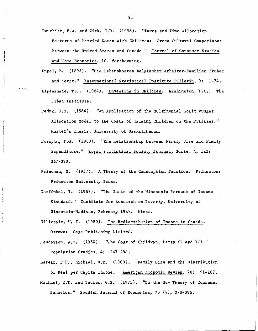
Douthitt, R.A. and Zick, C.D. (1988). "Taxes and Time Allocation
Patterns of Married Women with Children: Cross-Cultural Comparisons
between the United States and Canada." Journal of Consumer Studies
and Home Economics, 10, forthcoming.
Engel, E. (1895). '~ie Lebenskosten Belgischer Arbeiter-Familien fruher
and jetzt." International Statistical Institute Bulletin, 9: 1-74.
Espenshade, T.J. (1984). Investing in Children. Washington, D.C.: The
Urban Institute.
Fedyk, J.M. (1986). "An Application of the Multinomial Logit Budget
Allocation Model to the Costs of Raising Children on the Prairies."
Master's Thesis, University of Saskatchewan.
Forsyth, F .G. (1960). "The Rela tionship between Family Size and Family
Expenditure." Royal Statistical Society Journal, Series A, 123:
367-393.
Friedman, M. (1957). A Theory of the Consumption Function. Princeton:
Princeton University Press.
Garfinkel, 1. (1987). "The Basis of the Wisconsin Percent of Income
Standard." Institute for Research on Poverty, University of
Wisconsin-Madison, February 1987. Mimeo.
Gillespie, W. I. (1980). The Redistribution of Income in Canada.
Ottawa: Gage Publishing Limited.
Henderson, A.M. (1950). "The Cos t of Children, Parts II and III."
Population Studies, 4: 267-298.
Lazear, F.P., Michael, R.T. (1980). "Family Size and the Distribution
of Real per Capita Income." American Economic Review, 70: 91-107.
Michael, R.T. and Becker, G.S. (1973). "On the New Theory of Consumer
Behavior." Swedish Journal of Economics, 75 (4), 378-396.
53
Muellbauer, J. (1977). "Testing the Barten Model of Household
Composition Effects and the Cost of Children." Economic Journal, 87:
460-487.
Muellbauer, J. (1980). "The Estimation of the Prais-Houthakker Model of
Equivalence Scales." Econometrica, 48: 153-176.
Olson, L. (1983). Costs of Children. Toronto: Lexington Books.
Pechman, J.A. (1987). Federal Tax Policy, Fifth Edition. Washington,
D.C.: The Brookings Institution.
Pollak, R.A. and Wachter, M.L. (1975). "The Relevance of the Household
Production Function and Its Implications for the Allocation of Time."
Journal of Political Economy, 83 (2), 255-277.
Prais, S.J., and Houthakker, H.S. (1955). The Analysis of Family
Budgets. Cambridge: Cambridge University Press.
Price, D. W. (1971). "Unit Equivalence Scales for Specific Food
Commodities." American Journal of Agricultural Economics, 52:
224-233.
Ross, D.P. (1980). The Canadian Fact Book on Income Distribution.
Ottawa: Council on Social Development.
Rothbarth, E. (1943). "Note on a Method of Determining Equivalent
Income for Families of Different Composition." In C. Madge (ed.),
War-Time Pattern of Saving and Spending. Cambridge: National
Institute of Economic and Social Research.
Singh, B. (1972). "On the Determina tion of Economies of Scale in
Household Consumption." International Economic Review, 13: 257-270.
Singh, B., and Nagar, A.L. (1973). "Determination of Consumer Unit
Scales." Econometrica,4l: 347-355.
54
Sydenstricker, F., and King, W.I. (1921). "The Measurement of the
Rela tive Economic S ta tus of Families." Quarterly Publication of the
American Statistical Association, 17: 842-857.
Tedford, J .R., Capps, o. and Havlicek, J. (1986). "Adult Equivalence
Scales Once More--A Developmental Approach." American Journal of
Agricultural Economics, 68 (2), 321-333.
Theil, H. (1969). "A Multinomial Extension of the Linea.r Logit Model."
International Economic Review, 10: 251-258.
Tyrrell, T.J. (1979). "An Application of the Multinomial Logit Model to
Predicting the Pattern of Food and Other Household Expenditures in
the Northeastern United States." Doctoral dissertation, Cornell
Unive rsi ty.
Van der Gaag, J. (1982). "On Measuring the Cost of Children." Children
and Youth Services Review, 4: 77-109.
Van der Gaag, J., and Smolensky, E. (1982). "True Household Equivalence
Scales and Characteristics of the Poor in the United States." Review
of Income and Wealth, 28: 17-28.
Williams, R. G. (1986). "Development of Guidelines for Child Support
Orders." Washington, D.C.: Office of Child Support Enforcement,
U.S. Department of Health and Human Services.