Embed Size (px)
Citation preview

InstituProf. D
May 20
Superv
Elamod
ut für TDr.-Ing.
011
visors: J
aboradels o
hermiscH.-J. Ba
James S
ation oof sol
M
Mat
che Strauer, Or
Spelling
of thear gasplant
aster thof
tthias
römungrd.
g, Corin
ermo-es-turbts
hesis
Russ
gsmasc
a Höfle
econobine p
s
chinen
er
omic powerr


I hereby declare that I did this work independently, using only the listed sources and aids.
Karlsruhe, May 2011

Acknowledgment
I want to thank Prof. Torsten Fransson, head of the Department of Energy Technology at the Roy-al Institute of Technology for giving me the possibility to do my Master thesis at his institute. The same gratitude goes to Prof Bauer, head of the Institut für Thermische Strömungsmaschinen at the Karlsruhe Institute of Technology for supervising my work from Germany.
My sincerest appreciation goes to my supervisor James Spelling who’s competence and helpful-ness were highly appreciated and made this work possible and fun. I am equally thankful to the head of the solar group, Dr. Björn Laumert for his guidance and advice throughout the project.
I additionally want to extend my thanks to my supervisor at the Institut für Thermische Strömungsmaschinen, Corina Höfler for her crucial help and useful suggestions during the writing and correction process.
Last but not least I want to express my gratitude to my parents whose mental and financial support gave me once again the opportunity to study six wonderful months abroad.

Tab
List of
List of
Nomen
1 Intr
2 Bac
2.1
2.2
2.3
2.4
2.5
3 Ela
3.1
3.2
3.3
le of Co
f Figures
f Tables
nclature
roduction ..
ckground ..
Solar rad
2.1.1 D
2.1.2 C
2.1.3 S
Concentr
2.2.1 P
2.2.2 L
2.2.3 D
2.2.4 S
Conversi
2.3.1 T
2.3.2 T
The poten
2.4.1 C
The gas t
aboration of
The simu
The hybr
3.2.1 T
3.2.2 T
3.2.3 T
3.2.4 T
3.2.5 O
The comb
ontent
...................
...................
diation .........
Distribution a
Concentration
olar radiatio
rating Solar
arabolic trou
Linear Fresne
Dish design ..
olar tower p
ion of heat to
The Clausius
The Joule-Br
ntial of CSP
Cost analysis
turbine in C
f dynamic S
ulation softw
rid solar gas
The heliostat
The tower ....
The receiver .
The gas turbi
Other elemen
bined cycle
....................
....................
...................
and density
n of solar ra
on data ........
Power Syste
ugh plant ....
el plant ........
...................
power plants
o electricity
s-Rankine cy
rayton Cycle
P technology
s of a CSP pl
SP technolo
System Mod
ware TRNSY
turbine cyc
s field .........
...................
...................
ine ...............
nts ...............
...................
...................
...................
...................
of the solar
adiation .......
...................
ems ............
...................
...................
...................
s ..................
..................
ycle ............
e ..................
y and econom
lant ............
ogy .............
dels.............
YS ...............
cle ...............
...................
...................
...................
...................
...................
...................
...................
...................
...................
radiation ....
...................
...................
...................
...................
...................
...................
...................
...................
...................
...................
mic aspects.
...................
...................
...................
...................
...................
...................
...................
...................
...................
...................
...................
....................
....................
...................
...................
...................
...................
...................
...................
...................
...................
...................
...................
...................
...................
...................
...................
...................
...................
...................
...................
...................
...................
...................
...................
...................
...................
...................
...................
...................
...................
...................
...................
...................
...................
...................
...................
i
iii
vii
viii
.............. 1
.............. 4
.............. 4
.............. 6
.............. 6
.............. 9
............ 10
............ 10
............ 11
............ 11
............ 12
............ 16
............ 17
............ 19
............ 20
............ 22
............ 29
............ 32
............ 32
............ 34
............ 37
............ 40
............ 41
............ 43
............ 44
............ 45

3.4
4 Cos
4.1
4.2
4.3
5 Mo
5.1
5.2
5.3
5.4
6 Res
6.1
6.2
6.3
6.4
7 Con
8 Ref
Appen
A.1
3.3.1 T
3.3.2 T
3.3.3 O
Validatio
st calculatio
Cost func
4.1.1 T
4.1.2 T
4.1.3 T
Cost func
4.2.1 T
4.2.2 T
4.2.3 T
4.2.4 T
Data acqu
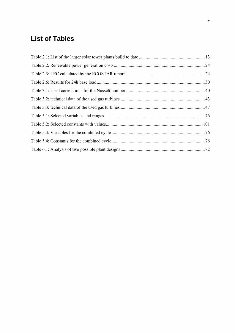
odel optimiz
Multi-obj
Evolution
The Queu
The optim
5.4.1 P
5.4.2 P
sult of the o
Evaluatio
Results f
Results f
Variation
nclusions an
ferences .....
ndix ............
1 One TRNS
The heat reco
The turbine ..
Other compo
on of the mo
ons ..............
ctions for th
The heliostat
The receiver
The power un
ctions for th
The HRSG u
The power un
The condense
The condensa
uisition ove
zation .........
jective optim
nary algorith
ueing Multi-
mization set
rogram desc
arameters ch
optimization
on of a multi
for the hybri
for the comb
n of the fuel
nd outlook .
...................
...................
SYS simulat
overy steam
...................
nents ..........
odels ............
....................
he hybrid cyc
s field .........
and the tow
nit ...............
he steam cyc
nit ...............
nit ...............
er and coolin
ate and feed
r TRNSYS .
....................
mization ......
hms .............
-Objective O
up ...............
cription .......
hosen for th
n .................
i-objective o
d cycle ........
bined cycle ..
price and th
....................
....................
....................
ion run .......
generator...
...................
...................
...................
...................
cle ..............
...................
wer ...............
...................
cle ...............
...................
...................
ng tower ....
dwater pump
...................
...................
...................
...................
Optimizer ...
...................
...................
he optimizati
...................
optimization
...................
...................
he heliostat c
...................
...................
...................
...................
...................
...................
...................
...................
...................
...................
...................
...................
...................
...................
...................
...................
...................
p ..................
...................
...................
...................
...................
...................
...................
...................
ion ..............
...................
n result ........
...................
...................
costs ...........
...................
...................
...................
...................
...................
...................
...................
...................
....................
...................
...................
...................
...................
...................
...................
...................
...................
...................
...................
....................
...................
...................
...................
...................
...................
...................
....................
...................
...................
...................
...................
....................
....................
....................
...................
...................
...................
...................
...................
...................
...................
...................
...................
...................
...................
...................
...................
...................
...................
...................
...................
...................
...................
...................
...................
...................
...................
...................
...................
...................
...................
...................
...................
...................
...................
...................
ii
............ 47
............ 49
............ 49
............ 50
............ 54
............ 54
............ 54
............ 55
............ 55
............ 56
............ 56
............ 57
............ 58
............ 59
............ 59
............ 63
............ 63
............ 68
............ 70
............ 74
............ 74
............ 75
............ 77
............ 77
............ 80
............ 86
............ 89
............ 93
............ 95
............ 99
............ 99

iii
A.2 Correlation of different tower materials ............................................................................ 101
A.3 Constants chosen for the optimization .............................................................................. 101
A.4 The MATLAB functions ................................................................................................... 102

i
List of Figures
Figure 1.1: Scheme of a solar thermal tower power plant ............................................................... 1
Figure 2.1: Definition of absorber and aperture on a parabolic trough collector .............................. 5
Figure 2.2: Acceptence range of a line and a point focusing system ................................................ 6
Figure 2.3: a) Theoretical achievable absorber temperature ............................................................. 8
Figure 2.4: Yearly Mean of Daily Irradiation in UV in the World ................................................... 9
Figure 2.5: Parabolic Trough Principle ........................................................................................... 10
Figure 2.6: Parabolic Trough Principle ........................................................................................... 11
Figure 2.7: Dish/Stirling scheme .................................................................................................... 12
Figure 2.8: Central tower system .................................................................................................... 12
Figure 2.9: Open air receiver scheme ............................................................................................. 13
Figure 2.10: An external receiver (left) and a cavity receiver (right) ............................................. 15
Figure 2.11: The ideal Carnot cycle ................................................................................................ 16
Figure 2.12: Theoretical total efficiency of a CSP system ............................................................. 17
Figure 2.13: The Clausius-Rankine Cycle in a T,s diagram ........................................................... 18
Figure 2.14: The Joule-Brayton Cycle in a T,s diagram ................................................................. 19
Figure 2.15: World primer energy demand ..................................................................................... 20
Figure 2.16: Online and planned CPS plants .................................................................................. 22
Figure 2.17: Cost for the Solar Tres components in percent .......................................................... 23
Figure 2.18: LEC prediction for two different scenarios .............................................................. 25
Figure 2.19: Breakout of the LEC ................................................................................................... 25
Figure 2.20: Predicted Heliostats Cost Improvements.................................................................... 27
Figure 2.21: Impact of innovations on solar LEC for the SCR system .......................................... 31
Figure 3.1: The information flow for a TRNSYS Type .................................................................. 32
Figure 3.2: Scheme of the hybrid solar tower power plant cycle .................................................. 35
Figure 3.3: The hybrid solar gas turbine cycle scheme and its model in TRNSYS ........................ 36
Figure 3.4: A Solar One Heliostat ................................................................................................. 37
Figure 3.5: the cosine effect on heliostats with different orientation .............................................. 38
Figure 3.6: The field efficiency ..................................................................................................... 39
Figure 3.7: The SOLGATE pressurized receiver .......................................................................... 41

ii
Figure 3.8: The SGT 750 (left) and the SGT 400 (right) ................................................................ 43
Figure 3.9: The plant scheme for the combined cycle .................................................................... 45
Figure 3.10: The simulation model of the combined cycle in TRNSYS ........................................ 46
Figure 3.11: Pinch point analysis for the SGT750 (upper figure) and SGT400 (lower figure) ...... 48
Figure 3.12: T,s diagram for the hybrid cycle at full fuel supplement firing .................................. 51
Figure 3.13: T,s diagram for the hybrid cycle during solar preheating .......................................... 52
Figure 3.14: T,s diagram for the combined cycle ........................................................................... 52
Figure 3.15: Sankey diagram for the SGT 750 in the hybrid cycle ................................................ 53
Figure 3.16: Sankey diagram for the SGT 400 in the hybrid cycle ................................................ 53
Figure 4.1: Cost distribution for the hybrid cycle, with two different solarization sizes ................ 60
Figure 4.2: Cost distribution for the combined cycle, with two different solarization sizes .......... 60
Figure 5.1: Data flow between MATLAB and TRNSYS ............................................................... 63
Figure 5.2: Expected optima in a single objective optimization ..................................................... 64
Figure 5.3: Illustration of a general multi-objective optimization problem .................................... 65
Figure 5.4: General data flow in an EA ......................................................................................... 68
Figure 5.5: Solutions at the start of the optimization(left) and after termination (right) ................ 69
Figure 5.6: Simplified data flow scheme during the optimization process ..................................... 74
Figure 6.1: Typical POF for the analyzed cases ............................................................................. 77
Figure 6.2: Breakup of the LEC ...................................................................................................... 78
Figure 6.3: Progression of the solar share with increasing solar field size ..................................... 79
Figure 6.4: Comparison of the initial gradient of Cinv and LEC ..................................................... 80
Figure 6.5: Solar share vs. LEC ..................................................................................................... 81
Figure 6.6: Solar share vs. LEC ...................................................................................................... 81
Figure 6.7: specific. CO2 emissions vs. LEC .................................................................................. 83
Figure 6.8: Fraction of the total energy generation , with SGT 750 base load as reference ........... 83
Figure 6.9: specific. CO2 emissions vs. LEC ................................................................................. 84
Figure 6.10: Solar share vs. Investment costs ................................................................................. 84
Figure 6.11: Solar share vs. heliostat area and tower height........................................................... 85
Figure 6.12: Total mirror area and solar share vs. receiver area ..................................................... 85
Figure 6.13: Solar share vs. LEC .................................................................................................... 87
Figure 6.14: specific CO2 emissions vs. Solar share....................................................................... 87
Figure 6.15: Solar share vs. investment costs ................................................................................. 88

iii
Figure 6.16: Fraction of the total energy generation ....................................................................... 88
Figure 6.17: Impact of the heliostat price on the LEC .................................................................... 90
Figure 6.18: Price development for natural gas during the last decade .......................................... 91
Figure 6.19: Solar share vs. LEC for three fuel prices .................................................................... 91
Figure 6.20: Solar share vs. specific CO2 emissions for three fuel prices ...................................... 92
iv
List of Tables
Table 2.1: List of the larger solar tower plants build to date .......................................................... 13
Table 2.2. Renewable power generation costs ................................................................................ 24
Table 2.3: LEC calculated by the ECOSTAR report ...................................................................... 24
Table 2.6: Results for 24h base load ............................................................................................... 30
Table 3.1: Used correlations for the Nusselt number...................................................................... 40
Table 3.2: technical data of the used gas turbines........................................................................... 43
Table 3.3: technical data of the used gas turbines........................................................................... 47
Table 5.1: Selected variables and ranges ........................................................................................ 76
Table 5.2: Selected constants with values ..................................................................................... 101
Table 5.3: Variables for the combined cycle .................................................................................. 76
Table 5.4: Constants for the combined cycle .................................................................................. 76
Table 6.1: Analysis of two possible plant designs .......................................................................... 82

v
Nomenclature Abbreviations CC Combined cycle CRS Central receiver systems CSP Concentrated solar power DLR Deutsches Zentrum Für Luft- und Raumfahrt (German Aerospace Department)DNI Direct normal irradiation EA Evolutionary algorithm ECOSTAR European Concentrated Solar Thermal Road-Mapping HRSG Heat recovery steam generator HTF Hot temperature fluid LEC Levelized electric cost M&S Marshall and Swift Index MMBTU One million British thermal units MOO Multi objective optimization MOP Multi objective problem NTU Number of transferred units O&M Operation and maintenance OSMOSE OptimiSation Multi-Objectifs de Systemes Energetiques integres POF Pareto optimal front PV Photovoltaic REFOS Receiver for fossil-hybrid gas turbine systems SOLGATE Solar hybrid gas turbine electric power system SOO Single objective optimization SOP Single objective problem STEC Solar thermal electric component library
Symbol Unit Meaning
Latin symbols
A m2 Area c - Concentration ratio cp J/(kg K) Specific isobare heat capacity C USD Cost E0 W/m2 Solar constant E kWh Energy, produced electricity F N Force h kJ/kg Enthalpy h W/m2K Heat transfer coefficient

vi
Ib W/m2 Beam radiation Kg/s Mass flow
n - Exponent
P / W Power
p bar Pressure r m Radius t s time T K Temperature
m3/s Volumic flow rate
V m³ Volume W Joule Work
Greek symbols
- Emissivity
- Heat exchanger efficiency
c - Carnot efficiency
- Optical losses
rad Acceptance angle ρ kg/m³ Density
S W/m2K4 Stefan-Boltzmann constant
Π - Pressure ratio
Indices
abs Absorber air Air ap Aperture aux Auxiliary comb Combustion chamber comp Compressor cond Condenser cw Cooling water dp Pressure loss eco Economizer el Electric evap Evaporation evap Evaporator fire Firing helio Heliostats max Maximum min Minimum

vii
net Net rec Receiver ref Reference rel relative sh Superheater sol Solar tower Tower turb Turbine

1 Intro
1 I
For theThe ineratingitive restaged sourcegeneranology
So far,to nowtions oof bothBraytocentratature fstored steam a singlpressedtemper
Figure(left) a
oduction
ntrodu
e short and mncreased demg prices for cenewable en
research aes, solar theration. In recy, solar towe
, almost all w several powof solar toweh configuraton Cycle on ted on the tofluid (HTF)in a storagecycle to runle working fd air. For corature.
e 1.1: Schemand in a Bra
ction
mid-term oumand for fosconventionanergy sourcand developrmal power pent years, a
er power pla
work concewer plants her power plations is displ
the right haop of a towe. In the Rane tank or dirn the turbinefluid. The reombustion in
me of a solaayton Cycle
utlooks a redssil resourceal power planes. To mak
pment are cplants are n
apart from thants were in
entrated on shave been suants based onlayed in Figand side. Su
er were a recnkine Cycle rectly passede and generaeceiver transn the combu
ar thermal e configurat
duced grow es will therents, eventuake these ne
critical. Connext to wind he already fthe focus of
solar tower uccessfully inn the Brayto
gure 1.1 , theunlight is coceiver absorb this is usuad on to the s
ator. The Brasfers the heaustion chamb
tower powetion (right)
rate in the wefore be accoally paving thew technolognsidering the
parks the onfairly well ef research an
systems basnstalled [1].on Cycle aree Rankine Collected by mbs the radiatally a moltesteam generayton Cycleat from the cber, fuel is a
er plant in
worlds energompanied byhe way for cgies ready fe potential nly possibili
established pnd developm
sed on the RIn this work
e investigateCycle on the mirrors calletion in orderen salt or mrator where
configuratioconcentratedadded to inc
a Rankine
gy demand iy further grcommerciallfor deploymof renewabity for bulk parabolic tro
ment.
Rankine Cyck, different
ed. The basicleft hand si
ed heliostatsr to heat a h
metal. The heit is transferon is characd sunlight tocrease the tu
Cycle confi
1
s unlikely. rowing op-ly compet-
ment, early ble energy electricity
ough tech-
cle, and up configura-c principle de and the s and con-ot temper-eat can be rred to the cterized by o the com-urbine inlet
iguration

1 Introduction 2
Using a gas turbine in such central receiver systems has a number of consequences that can be critical for a deployment decision, when taking into account local geographic and politic re-strictions.
High operation temperatures. Substitution of the steam turbine cycle with a gas turbine driven cycle allows higher operating temperatures and therefore a higher efficiency of the power plant.
No cooling water. In an open Brayton cycle with air as heat transfer medium, waste heat can be discharged to the environment without additional cooling. Already installed con-centrating solar power (CSP) systems using a steam cycle have a high demand of cooling water. A resource that is particularly scarce in regions where the solar power plants are most beneficial, as e.g. in arid areas.
Hybrid configuration. In the absence of a storage device or for a quick response to varying solar input, a constant power output can only be achieved with supplemented fossil fuel burning. Although this cannot be an objective on the long term, it is an important instru-ment to minimise investment risks and boost the deployment of gas turbine driven power plants today.
Combined cycle. Due to the high gas turbine outlet temperatures, the integration of a com-bined cycle can further rise the efficiency whilst reducing the costs for the solar generated energy1. Apart from the combined cycle other promising options are the combination of a Brayton cycle with cogeneration, cooling or desalination.
The integration of a gas turbine in a CSP system has up to now only been tested in experimental power plant setups [2]. No plant on a commercial scale has been built yet. Therefore it is im-portant to have a broad knowledge of the thermodynamic potential and limits, as well as of the expected costs for investment and operation of the plant.
In this work two different gas turbine driven CSP plants were simulated, using the software tool TRNSYS. More precisely, a special model library, the TRNSYS Model Library for Solar Thermal Electric Components (STEC) developed by the German aerospace agency (DLR) is implemented. The cycles are:
I. Hybrid gas turbine solar cycle
II. Combined cycle
The hybrid cycle uses heat from concentrated solar radiation and from supplemented firing of fossil fuel to drive the gas turbine. The more heat is provided by radiation the less additional fuel is needed. The combined cycle also uses the hybrid system but adds a steam generation unit and a steam turbine, using the exhaust heat from the gas turbine.
1Cooling water would now be required for the steam cycle. However, the demand is considerably lower than in a pure Rankine based CSP.

1 Introduction 3
With the thermodynamic data from the models and a set of corresponding cost functions for each component in the cycles, predictions about the power plant performance will be derived. These include:
Overall investment costs: The sum of all costs accumulating during construction
Levelized electric costs (LEC): A figure that spreads all costs that accrue over the life-time of the plant divided by the annual electric output.
Solar Share: The percentage of electric power that comes from solar energy.
CO2 emissions: The amount of CO2 per kWh that is discharged to the environment
In a next the step, an optimization was performed to find optimal configurations of the plant mod-els. As it is often the case for energy system optimization, problems are multi-objective. Highest efficiency is desired for minimal costs, or maximal power output for minimal CO2 emissions. The result is a trade-off curve which offers several equally valuable solutions.
In this work, a multi-objective evolutionary algorithm was used to perform the optimization and obtain a number of trade-off curves for the two plant configurations. Trends were analyzed for various cases.

2 Back
2 B
In thisby an otion is tems is
2.1
To detphysicitself asion atlayer, c5670 Kyieldin
where distancextrate
with over th
Scattertion pohas to the air the atmdry dathe soles valu
kground
Backgro
s chapter somoverview ofanalyzed. F
s reviewed.
Solar r
termine the cal propertieand its relatit a temperatucalled the phK. The specng
is the emce 1.4errestrial val
the radius he year at ar
ring processower that retravel throumass coeffi
mosphere anay. The highlar radiationues of 2200
ound
me fundamef the CSP teFinally, the w
radiation
amount of s of the sunive position ure of arounhotosphere.
cific power
missivity, 469 10 lue of E0, ca
of the sun. Bound 1.7%.
ses as well aeaches the suugh the atmoicient (AM)
nd the distanher the AM n that can be
⁄ to 2
entals requirchnology. Twork accom
n
energy that nlight is nece
to the earthnd 107 K andHere, the suon its surfa
the Stefan- of the su
lled the sola
Because of tIt is measur
as absorptionurface of theosphere and . It is the quce that the licoefficient, collected fl
2800 ⁄
red for solarThe potentia
mplished so f
can be obtaessary. Thesh. The sun gd transfers ituns radiatio
ace ps can be
6.24
-Boltzmann un to the eaar constant.
the eccentricred by satell
1.353 2
n in the atme earth. It dthe cloudine
uotient of theight has to tthe weaker
luctuates wit in the most
r engineerinal in context far in the fie
ained from sse in turn degenerates its t with severn resemblese calculated
4 10
constant anarth, the pow
city of the eite to be [3]
21
mosphere defepends mainess of the ske actual travravel with thr is the irradth time and t favorable r
ng are brieflyto the actua
eld of gas tur
solar radiatiepend on theenergy in thal different
s a black bodd with the S
nd T the temwer of the su
arth’s orbit,
fine the fracnly on the eky. This distelled distanche sun in thediation. Therlocation. Onregions of th
ly describedal global ene
urbine driven
ion, knowlee properties he core by nprocesses tody at a temp
Stefan-Boltzm
mperature. Dunlight redu
its value flu
ction of specextent, whichtance is indice of the lige zenith on arefore, the fn a clear dayhe earth (see
4
d, followed ergy situa-n CSP sys-
dge of the of the sun
nuclear fu-o the outer perature of mann law,
(2.1)
Due to the uces to the
(2.2)
uctuates
(2.3)
cific radia-h the light cated with ht through a clear and fraction of y, it reach-e also Fig-

2 Back
ure 2.4effectiveratingthe fol
Here, tsorber
the facfer coe
F
Figureapertursorber.tion ofcollectcomingimum dianceAabs A⁄
c = 30quenceconcenthe accrange f
kground
4 and Figurve the less h
g temperaturlowing simp
the apertureAabs, where
ctor that reduefficient.
Figure 2.1: D
e 2.1 illustrare of the co. Radiation of the solar rator without g radiation otemperature
e can only Aap. To use t
0 are requiree, the acceptntration qualceptance angfrom which
re 2.16). Thheat it losesre and the aplified energ
e Aap is the e it is conve
uces the bea
Definition o
ates the geomllector. In thoutside the aadiation is nconcentratioof 800 ⁄e of 44 canbe obtainedthe solar rad
ed, and an otance angle olity of the ragle range of the receiver
Receiver
e thermal c to the envir
absorber areagy balance [4
area that therted into us
am solar radi
of absorber
metry of a phis case the acceptance anecessary toon, e.g. a so
, assumingn be reachedd with smadiation in a c
order of maof the systemadiation depf the receiverr will accep
onversion taronment. Tha. The useab4]
he concentraseful heat re
iation by
and apertu
parabolic trreceiver co
angle cannoto increase tho called flatg values for d. Considera
aller values conventiona
agnitude higm is reducedpends on ther. The highe
pt radiation.
akes place ihe heat losseble thermal
ator can use educed by lo
the optical l
ure on a par
ough collecnsists of an t be reflecte
he maximumplate collec
1 andably higher for and a
al steam cycl
gher for a gad. As it wille power denser the concenFor high co
in a collectoes rise propopower c
to focus theoses in the a
losses, h rep
rabolic trou
tor. The conevacuated g
d on the recm temperaturctor should
0, with temperaturea higher cole, concentra
as turbine cl be seen latesity distributntration, the ncentrations
Concentrato
or, which isortionally wcan be dete
e radiation absorber itse
presents the h
ugh collecto
ncentrator dglass tube a
ceiver. The cre of the recreturn 80% equation (2
es with terreoncentrationation values
cycle [5]. Aer in section
ution of the ssmaller is th
s it is theref
or
5
s the more with its op-
rmined by
(2.4)
on the ab-elf. is
heat trans-
or [5]
defines the and the ab-concentra-ceiver. If a
of the in-.4) a max-
estrial irra-n ratio
of at least
s a conse-n 2.1.2, the source and he angular
fore neces-

2 Back
sary tosorber
2.1.1
Since tparallepears owould tance fdesignsun’s iena is Scatterlar ranwell abradiatiticles avalues tratingceptantem wenergy
2.1.2
With tcan be
kground
o adjust this can only be
Distribu
the sun has el but has a on an angle be constant
from the cenn of central rimage produalso called lring in the a
nges. In closebove the radon, CR. If sa slight hazeof CR, the
g system, bence angle of ith the same
y gain from t
Figur
Concent
the help of a increased. T
Reduction operating t
A better utem
range in rele achieved w
ution and d
a finite distslight diverof 16′. If tht. However, ntre increasreceiver systuces a hot splimb darken
atmosphere oe proximity diation of thscattering efe can be obsbeam radiatcause of a t
= 4.65 me angle , the the irridi
Line focu
re 2.2: Acce
tration of s
additional deThis is motiv
of the spectemperature
utilization of
lation to thewith beam ra
ensity of th
ance from thrgence. The he sun was a
since the des, the sun tems as needpot with highning. The intof the earth of the sun’se remaining
ffects increaserved. This tion Ib contatoo small acmrad (=16‘) not all of th
iance is high
using system
ptence rang
olar radiat
evices such vated by the
ific heat loss (Eq. (2.4)
f the expens
e position ofadiation and
he solar rad
he earth (dse
geometric a lambertiandensity and tis slightly d
ded in CSP ther radiativetensity decreresults in an
s disk, the rag hemispherese due to higleads to an
ains shares, tcceptance an
the losses ehe CR is loher for point
m
ge of a line
tion
as mirrors oe following a
ses at the in
ive absorbe
f the sun. Hea collector s
diation
e), its solar rexpansion o
n emitter, thethe temperatdarker at thetower plantse flux than teases towardn additional adiation is ore of the skygh cloud layincrease in tthat usually
ngle. For a pequal the vast. Therefort focusing th
Point focu
and a point
or lenses, thaspects:
nput aperture
r unit, reduc
ence, high tesystem using
radiation reaof the sun ae distributionture of a stae edges. This because thehe overall ads the edgesradiation in
rders of mag. This effectyers (cirrus)the circumsocannot be c
point focusinlue of CR. Ire the influehen for a line
sing system
t focusing sy
e irradiance
e of the rece
cing the spe
emperaturesg a tracking
aching the eas seen fromn of the angar diminish is is importae central reg
average. This by the factnput from lagnitude lowet is called ci), aerosols orolar radiatiocollected by ng system wIn a line focence of the Ce focusing sy
m
ystem [4]
e of the solar
eiver, resulti
ecific costs o
6
s at the ab-device.
earth is not m earth ap-gular range as the dis-ant for the gion of the s phenom-tor 2.5 [6]. rger angu-er, but still ircumsolar r dust par-
on. At high a concen-
with an ac-cusing sys-CR on the ystem.
r radiation
ing in high
of the sys-

2 Background 7
The possibility to oversize the collector system for an integration of a storage device
If it would be possible to increase the concentration to any level, one would at some point reach higher temperatures than found on the sun’s surface, which is physically impossible2. Therefore, from a thermodynamic point of view, a limit to the concentration must exist. As seen above, a smaller receiver, resulting in a higher concentration ratio, leads to a smaller acceptance angle. If this angle is reduced further, losses will occur. This limit can be used to calculate the concentra-tion limit (see also [5]). A perfectly aligned collector transfers the radiated power PS-E to the re-ceiver
(2.5)
where TS is the temperature of the sun. Equation (2.1) applied on the receiver yields to the follow-ing radiation from the absorber to the sun
(2.6)
Likewise it applies
→ (2.7)
With the earlier introduced concentration ratio c ⁄ and equation (2.7), the maxiumum
for c can be expressed as
,1
(2.8)
If is assumend to be 16′, the concentration maximum for a two-dimensional concentrator is
, 45000 (2.9)
For a one-dimensional or line concentrator it can be shown that the maximum concentration ratio is limited to
,1
212 (2.10)
With an absorber temperature Tabs lower than TS, but without any heat gain (efficiency 0), the following concentration ratio c can be derived for a perfect concentrator
lim→
(2.11)
2 This situation would result in a heat flux from a colder to a hotter source, which is a violation of the second law of thermodynamics.

2 Back
This cture Ta
Figuretrationcan bereceive
Figuretion ratration
With aefficienefficienthe recrises. Topticalpointlewould accuraentire length.trance.ture grcentratvalue.
kground
onsideration
abs
e 2.3a showsn ratio. Evene reached. Iner concentra
e 2.3: a) Thatio b) collen ratios [5]
an increasinncy increasency. The receiver area iThe achievabl accuracy oess to adjustbe lost due
acy for the syaperture. Op. The mirro. This is espradients are tion ratio is
n and the as
s the theoretn with low cn Figure 2.3ation ratios i
heoretical aector efficie
g concentraes in accordaason is that is smaller thble concentrof the systemt the concentto inaccuracystem. Espeptical errorsr system th
pecially impohigh, as it isa comprom
sumption of
tically achieconcentration3b the collecs shown.
achievable aency as a fu
tion ratio c,ance with thwith a high
han the radiaration ratio dm itself. In tration ratio cies. The higecially in mis of the outeerefore prodortant for ths the case fo
mise of all re
f a black bo
evable absorn ratios relactor efficien
absorber teunction of te
, a higher abhe concentraher c the coation lossesdepends nota mirror araccording t
gher the conirror arrays er mirrors haduces a unif
he design of or gas turbinelated effect
ody leads to
rber temperaatively high ncy as a func
mperatureemperature
bsorber temation ratio c. nvective he, which incrt only on therray with reto the solar ancentration, the acceptanave a biggerform distribthe receiver
ne driven solts, but often
the maximu
ature as a futheoretical action of tem
as a functie for differe
perature canIf Tabs is co
at losses derease as the e acceptancelatively largangle, since the higher ince angle is r impact due
buted radianr when templar plants. Tthe econom
um absorber
unction of thabsorber tem
mperature fo
ion of the cent absorbe
n be achieveonstant, c incecrease faste
absorber tee angle but age optical emuch of the
is the requires not constanue to the incrnce at the reperatures andThe choice omic factors d
8
r tempera-
(2.12)
he concen-mperatures or different
concentra-er concen-
ed, i.e. the creases the er, because emperature also on the rrors, it is e radiation ed level of nt over the reased run
eceiver en-d tempera-of the con-dictate this

2 Back
2.1.3
A crucmationing syovervible infin Euro
RadiatcommoTRNSYal Solato distiis genedata haexact uical elerepresefor a wplants amounance. Awith vis not tpossib
kground
Solar ra
cial elementn about the istems, becaew about thfrastructure ope, like Sp
Figur
tion data is on, a monthYS, data filear Radiationinguish it froerally less aas an accuraup to 5% ements, sucents the aveworst case sbased on th
nt of aerosolAlthough theariations of taking into ale.
adiation dat
t for a reliabirradiance atause only thhe irradianceand high irrain, Portuga
re 2.4: Year
usually avahly average des for a typi
n Data Base oom the earli
accurate due acy no bette[3]. The TMh as ambien
erage valuescenario. Thhis data. Anls in the atme global effe16% at som
account the l
ta
ble solar powt the desiredhe beam rad variation ar
radiance areal and Greec
rly Mean of
ailable for hdaily total raical meteoroof the Uniteer TMY datto poorer in
er than 10MY2 are datant temperatu of many ye
his has to benother effectmosphere in tect is small,
me places dulast 20 years
wer plant sid location. Thdiation contrround the w
e the westernce.
f Daily Irra
horizontal suadiation and ological yeared States areta, taken fromnstrument q% or worsea sets of houure or wind ears, it is noe kept in mit that mightthe last deca it has been
uring the lasts, deviation
mulation is his is of parributes to th
world, measun states of th
adiation in U
urfaces as a an hourly to
r (TMY) dere available. Tm the years uality and c
e, whereas reurly values ospeeds for
ot suitable find when dit reduce simades, havingfound that l
t 25 years [9to the actua
the availabiticular impo
he heat gainred by satellhe US and t
UV in the W
function ofotal radiationrived from thThe data set 1950-1975.
calibration stecent measuof solar radiaa one year p
for simulatinimensioning
mulation accug a direct imlarge local f9]. Given thel insolation
ility of detaortance for cn. Figure 2.4llite. Areas wthe southern
World [7]
f time. Twon. In the sofhe 1961-199is known as Data from ttandards. Murements areation and mperiod. Sincng extreme g componenturacy is the
mpacting on fluctuations e fact that Tat a certain
9
ailed infor-concentrat-4 gives an with a usa-n countries
o types are ftware tool 90 Nation-s „TMY2“ this period
Most of this e probably
meteorolog-ce the data conditions ts for CSP e changing the irradi-can occur,
TMY2 data location is

2 Back
2.2
In the generafocusinkilowathe comradianting to r
2.2.1
Paraboformed
ment. If it isdirect ture limthe soldensity
ParaboEnergyare cocosts fthe LSwhich
FigurePrinci
kground
Concen
following sation is giveng systems. atts for smalmbination ot intensity, Crequirement
Parabol
olic trough pd like a para
The maximus heated to oevaporationmit and redular field depy changes in
olic trough py Generatingnsidered as
for the parabS-3 collector
increased w
e 2.5: Parabiple
ntrating
section a brien. In genera
CSP plantsll villages tof a heat storCSP plants ats and econo
ic trough p
plants belongabolic dish
um operatioover 400
n systems, efuces heat losending on w
n the two-ph
plants have g Systems) a „proven
bolic shape, r used in the
wind loads to
bolic Troug
Solar Po
ief overviewal, it can bes can be deso grid connerage device oare ready foomical aspec
plant
g to the lineand concen
antocothcuchToab
Twtitirain
on temperatudecomposin
ffectively elisses and inveweather and ase-flow in
the highest plants in Ctechnology“further up sc
e latest SEGo unacceptab
h
ower Syst
w over the de distinguishsigned for a ected applicaor hybridiza
or use in bascts.
e focusing syntrated on thnd 100 are or, used in thoncentrationhermodynamuracy of thehronization
The core elemf the mirrobsorber and
The steel tubwhich has thion. The steeive layer toange of the nfra-red rangure is limiteng will occuiminating thestment costtime of daythe absorber
maturity of alifornia op“ by projeccaling is als
GS plant hadble values.
tems
different typhed between
large poweations with
ation by runne load, as w
ystems. Radihe receiver. achieved [1he ANDASOn ration of mic limit, the tracking syof the entir
ment is the rrs. It contaicarries the H
be is embode function toel tube is us
o guaranteesolar spectrge to minimd by the HT
ur. One wayhe need of a ts. However, difficultiesr pipe.
f all CSP tecperating succct investorso limited by
d an increase
pes of CSP tn line focusir range, starseveral hundning the plan
well as in pea
iation is collConcentrati
10]. The EUOL 1 and 2 p82 [11]. B
his ratio is cystem, the ore system anreceiver systins a steel HTF.
died in an eo minimize
sually coateda high abs
rum and a smize the heaTF, which isy to overcomHTF. This i
r, due to insts are impose
chnologies, wcessfully for[12]. Howe
y wind loadsed aperture f
technology ing systems rting from odred megawnt on fossil fak load mod
lected in theion ratios b
UROTROUGplants in Sp
Beside the tconstrained boptical errornd the resultem in the litube which
evacuated glosses due t
d with a spesorption ovesmall reflectat loss to ths usually a tme this limiincreases thetationary coned by heat tr
with the SEr over 30 yeever, besides. The advanfrom 5.76m
10
for power and point
only a few watts. With fuel at low de, accord-
e reflector, etween 30
GH collec-pain have a theoretical by the ac-s, the syn-ltant costs. near focus works as
glass tube, to convec-
ecial selec-er a large tion in the e environ-hermo oil. t is to use e tempera-nditions in ransfer and
EGS (Solar ears. They s the high
ncement of to 10.3m,

2 Back
2.2.2
Fresneone paincreasthe Pla
isolatependenthe samregardally deinal pomirrorof viewlarmunfield co
2.2.3
The sodecentlarge rapplicamirror makingenginetor. A
Figu
kground
Linear F
el systems coarabolic concse the conceataforma So
ed by a glasnt of the emime for all ming controlli
efocusing soosition with s. On the otw, which is ndo the advaompared to
Dish des
olar dish systralised systerange of depation. Incomsystem, usu
g dish systee, convertingA Brayton cy
ure 2.6: Par
Fresnel pla
onsist of sevcentrator. Thentration ratilar de Alme
s plate and ission, are a
mirrors whicing this is n
ome mirrors time, makin
ther side, onwhy mirror
antages of thparabolic tr
sign
stem is a poem, with ev
ployment varming radiatioually measuems the mosg it into mecycle using a
abolic Trou
nt
veral segmenhis reduces tio because b
eria (PSA) re
the seconda more impor
ch makes a ot desirable,would not bng a readjus
ne servomotors are grouphe Fresnel syough [13].
oint focusingvery dish coriations as inon is reflectering betweet efficient Cchanical worturbine to e
ugh Princip
nted mirrorsthe costs of bigger aperteached a con
Nova171, mThis an acis sothe rarea. er ofalwayrangesure junnees duatedthe F
ary receiverrtant issue. Tcoupling to , because an
be possible. Astment neceor for each mped in arrayystem lead t
g concentratnverting solndividual poed and conc
en 50m2 -150CSP technolork and finalexpand the w
ple
s in close prthe mirrors,ures are posncentration
atec BioSol imainly by a requires a h
ccurate tracklved with areceiver, inCompared t
f the Fresnys receivinge thus the injoints as nee
ecessary. Whue to convecglass tube a
Fresnel syster. Therefore,The angular one conjoin
n adjustmentAdditionallyssary. This mirror is not
ys connectedto a cost red
tor. Unlike lar radiationower generacentrated to 0m2. Concenogy [14]. Thlly to electriworking flui
roximity to t, facilitates tssible. The dratio of 107in Lorca achsmaller diam
higher qualiking system. a secondarycreasing thto a parabol
nel collectorg radiation frnstallation oeded in parahile in parabction are suand radiatioem the hot , convectionvelocity of
nt servomott of the outpy, mirrors cawould be eat feasible frod to one motduction of ab
all the othern to electric ators or in a the power cntration ratihe heat is trac power in tid has also b
the ground, their handlindemonstratio7. The test chieved a ratmeter of theity of the m Usually thi
y concentrathe effectivelic system, tr remains
from the samof flexible habolic plantbolic troughuppressed byon losses doabsorber pi
n losses thatf the trackingtor possible.put power byan vary fromasier for sinom an econo
otor. Accordbout 50% fo
r CSP systepower. Thilarge scale
conversion uios can go uransferred tothe connectebeen tested.
11
instead of ng and can on plant at ollector of tio of even e tubes [5].
mirrors and is problem tor around e absorber the receiv-stationary,
me angular high pres-s becomes
hs the loss-y a evacu-
ominate, in pe is only t are inde-g system is . However y individu-m the nom-ngle driven omic point
ding to So-or the solar
ems, it is a is allows a connected
unit by the up to 4000, o a sterling ed genera- Electrical

2 Back
output 30 kWhave a
2.2.4
This pare mir
which exchancapacitheliostbine attime op
3 This is
Figure
Figure
kground
in the curreW for the Braalso been dem
Solar tow
oint focusinrrors that tra
circulates thnger by the Hty factor, wtat field enabt the design peration.
s mainly beca
e 2.7: Dish/S
e 2.8: Centr
ent dish/engayton systemmonstrated [
wer power
ng system coack the sunl
hrough the HTF and pr
while runninbles the systpoint. This
ause of the mo
Stirling sch
ral tower sy
gine prototypms under con[15]. Problem
etroomvoaaptho
plants
oncentrates ight around
tower. An aroduces elecg the plant tem to feed enables ch
odular setup th
heme
ystem
pes is aboutnsideration. ms arise fro
every dish haracking syst
other hand, wone system, maintaining very beginnionly very feare in direct and it therefopenetration che efficiency
opment and m
the sunlighttwo axes wSince all hdo not appvidual helual paraboof centrallower thavalues of ed sunlighabout 100stats. Here
attached powctric power.
at low insoenergy into
harging of th
hat also domin
t 25 kWe foSmaller dism the increa
as its own potem that cawhen an arrit never hasindividual uing of theirw experimeconcurrenc
ore remains can be achievy to over 30might help t
t with the hewith a mirror
heliostats arproximate onliostat approola. Thus, thl receiver s
an that of p500 to 1500
ht is sent to tm height, dee, the absorbwer cycle usUsually, a s
olation levelthe storage
he storage w
nates in PV po
r dish/Stirlinh/Stirling syased need fo
ower converan move theray of manys to shut dounits. Dish sr commerci
ental setups e to Photovto be seen i
ved. Howev0% seem to bo boost furth
elp of so calsize of usua
re located inne single pa
oximates a sehe achievabsystems (CRparabolic di0 in practice the receiver epending onber transfersses the steamstorage is incls or at nightanks, while
without a po
ower plants.
ng systems ystems of 5 or maintenan
rter and the e heavy un
y units is conown complesystems are ial introducin place so
voltaic (PV)if a noticeab
ver, strong inbe a promisher deploym
lled heliostally 50m2 -1n the same parabola, but egment of a
ble concentrRSs) is sigish systems [18]. The c
r situated in n the numbes the energym generated
ncluded to inht-time. An e still runnin
ower drop du
12
and about to 10 kWe
nce since
costs for a it. On the nnected to
etely while still at the
ction, with far. They
) systems3, ble market ncreases in sing devel-ment [16].
tats. These 50m2 [17]. plane they each indi-
an individ-ation ratio gnificantly , reaching
concentrat-a tower of
er of helio-y to a HTF d in a heat ncrease the
oversized ng the tur-uring day-

2 Back
Table plant fbe com
Key cgeneraal tempdition,performreceivebut alsequally
kground
Table 2.
Power
SSP
EURE
SUNS
Solar
CES
MSEE/
THE
SPP
TS
Solar
Cons
Solg
SierraSun
PS
PS2
Solar
2.1 gives anfeed electricmmercially o
component iated heat fluxperatures de the materiamance cycleer fits best tso on perfory developed
Open air r
.1: List of th
r Plant P
PS
ELIOS
HINE
r One
SA-1
/Cat B
MIS
P-5
SA
Two
sular
gate
n Tower
10
20
Tres
n overview al power int
operated.
in the solarizx densities oemanding hial must not es in the ranto a certain rmance and
d variations:
receiver
Figu
he larger so
Power(MWe)
0.5
1
1
10
1
1
2.5
5
1
10
0.5
0.3
5
11
20
17
of the existto the grid. S
zation proceof 0.3 – 4MWigh standardonly be ablenge of minuplant, depen
d costs requi
ure 2.9: Ope
olar tower p
HTF
Liquid Sod
Steam
Steam
Steam
Steam
Nitrat Sa
Hitec Sa
Steam
Air
Nitrat Sa
Pressurized
Pressurized
Steam
Air
Steam
Molten s
ting tower pSolar Tres i
ess is the reW/m2 the re
ds for the stre to absorb utes withoutnds very mu
uirements. F
en air receiv
plants build
Coun
dium Spa
m Ital
m Japa
m US
m Spa
alt US
alt Fran
m Rus
Spa
alt US
d Air Isra
d Air Spa
m US
Spa
m Spa
salt Spa
plants. Todays planned to
eceiver. Becaceiver must
ructural desihigh peak f
t damage ovuch on the cour types o
ver scheme
d to date [19
ntry
ain
ly
an
S 19
ain
S
nce
sia
ain
S 19
ael
ain
S
ain
ain
ain Under
y only the Po be the first
ause of the be able to cgn of the re
flux densitiever a long pconnected pof receivers
9], [20], [14]
Year
1981
1981
1982
982-1986
1982
1983
1984
1986
1993
995-1999
2001
2002
2009
2007
2009
r construction
PS10 and PSt power plan
concentratiocope with hieceiver set [2es but also eperiod. Whicower generacan be con
13
]
S20 power nt that will
on and the gh materi-22]. In ad-endure fast ch type of ation cycle nsidered as

2 Background 14
A blower sucks ambient air through the porous absorber material, which is heated up from the concentrated radiation. The absorber can be made from metallic or ceramic material. The hot air transfers the heat via an exchanger to the steam cycle. The use of air at ambi-ent pressure makes this design cheap and very easy to handle and maintain. Segments of the receiver can be replaced without pressure reduction if a modular layout is installed, giving the system a high operational availability. However, the low specific heat as well as the low pressure limit the heat transfer, requiring high air mass flows [5]. Figure 2.9 il-lustates the 200 kWth HiTRec-II open volumetric air receiver, tested at Plataforma Solar de Almería (PSA) in 2001. It worked with an inlet flux of up to 900 kW/m2 and an aver-age outlet air temperatures of up to 840°C with a peak outlet air temperatures of up to 950°C.
Closed air/helium receiver
To increase the transferable heat load, the air circulating through the receiver can be com-pressed. The concentrated solar radiation enters the receiver through a quartz window which has to withstand the high thermal loads and rapid temperature changes as well as the pressure difference to the environment with minimal reflection and absorption losses. This type will be discussed in detail in chapter 3
Direct evaporation receiver A directly evaporating absorber is for example implemented in the PS10 plant, working with a saturated steam cycle at 40bar and 250ºC. Although water has a much higher spe-cific heat capacity than air, water chemistry can result in problems when reaching very high temperatures. Therefore the heat flux to the receiver as well the pump performances have to be critically observed at all times. Failure to do so can lead to steam explosions if critical temperatures are exceeded. Another problem are the high costs for the storage of steam, when compared to molten salts [23].
Molten salt/metal receiver Molten salt or metals offer a high heat transfer coefficient at a low temperature differ-ence. Their high thermal conductivity reduces the thermal stress for the absorber material. Since the heat transfer occurs in a single-phase regime, the design of the receiver unit is less complex. An advantage is their high heat capacity at relatively low costs, making them an ideal medium for a heat storage implementation [23]. Molten sodium can be used for temperatures up to 880 combinded with an excellent thermal conductivity, leading to low absorber temperatures. As in air receivers, a heat exchanger is needed to transfer the heat to the steam cycle, increasing complexity and costs compared to direct evapora-tion systems. High temperature loads over a long period of time can lead to partial disso-ciation of the molten salts, resulting in fire hazards due to oxygen formation or toxic by-products like potassium nitrite. In steel pipes corrosion must be considered and is usually

2 Back
Two pternal aroundterminthe HTconfigu
A cavity. Thetrated the recty alloefficien
4 The fireceiver
kground
reduced byis pyropho
possibilities tdesign with
d the tower. ned by the mTF. Thereforuration base
Figure 2.
ity receiver te effectivenein Figure 2.
ceiver is not ows to trap tncy than the
figure illustrater system.
y special coaoric in air ab
to install theh the absorbe
To minimizmaximum tere, a systemed on a wate
.10: An exte
tries to miniess is determ.104, where axially sym
the solar rade external ty
es a cavity de
atings for pipove 140 [
e receiver oner in a 360ze heat lossemperature o
m which useser/steam med
ernal receiv
imize heat lomined by the
blue represmmetrical, thdiation morepe.
esign from a d
ipe walls. Co[5].
n the towerdegree arranes, the size iof the absorbs a molten sdia, which re
ver (left) an
osses to the e angle undeents the low
he acceptance effectively
dish collector
ontact with a
do exist: exngement allis reduced tber tubes analt or metal educes heat
d a cavity r
environmener which the west, and redce angle is my and conse
system. The
air must be a
xternally or ows for a co a minimumnd the heat HTF can blosses.
receiver (rig
nt by placingreceiver is i
d the highesmuch smallerquently the
effect shown
avoided, sin
inside a cavcircular helim. The limremoval cape build sma
ght) [24] [25
g the absorbinstalled. Thst temperatur. Howeverreceiver ha
is the same f
15
nce sodium
vity. A ex-iostat field
mits are de-pability of
aller than a
5]
ber in cavi-his is illus-ures. Since r, the cavi-as a higher
for a central

2 Back
2.3
One oknowncheap for CSJoule-Bconsistin a T-
At thereleasethe tota
It can bany heinput sambien
5 The dgenerat
6 Paraboin [18]
kground
Conve
f the majorn and tested and reliable
SP technologBrayton cycts of two iso-s diagram.
upper temped. The cyclal heat input
be shown theat to mechashould be prnt temperatu
downside of thion, making c
olic dishes are.
rsion of h
r advantagesheat transfe
e standard apgy, which wcle. Both areothermal and
perature TH,le efficiencyt Qth that is
hat the Carnoanical energrovided at aure to achiev
his situation icompromises i
e usually com
heat to el
s of solar per cycles canpplications f
will be explae variations od two isentro
Figure 2.11
, heat is addy C is indepconverted to
ot cycle effigy conversioa very high tve a high co
s that power in terms of eff
mbined with a S
lectricity
power towern be used, thfor the pow
ained in the of the ideal Copic change
1: The idea
ded to the fpendent of tho work W w
iciency is eqon process temperature
onversion eff
equipment is ficiency and d
Sterling cycle
y
r systems ishus enabling
wer generatiofollowing, Carnot cycles of state6. F
al Carnot cy
fluid and at he working
which can be
1
qual to the th[24]. As a c whereas heficiency. Ho
to date not ”desired power
e. Detailed info
s the fact thg the system
on5. The twoare the Claue. This is a rFigure 2.7 sh
ycle
the lower tefluid and decalculated a
heoretical mconsequenceeat removal owever, for t
off the shelf”output inevita
ormation abou
hat conventim to be equio most relevusius-Rankinreversible prhows the Ca
emperature escrbes the fas
maximum effe of this equshould occu
the applicati
” for solar theable.
ut this cycle c
16
ional, well ipped with vant cycles ne and the rocess that arnot cycle
T0 heat is fraction of
(2.10)
ficiency of uation heat ur close to ion of heat
ermal power
can be found

2 Back
enginewith in
The pr
describsion ofplottedratio ccalculacan beperformthe effhigher
Figurework aand an
2.3.1
The ClIt has bstood pcycle g
1→2 I
kground
es in CSP syncreasing tem
roduct of bot
bes the perfof mechanicad as a functic and differeation the upe seen, theremance can bficiency. This the theor
e 2.12: Theoas the functn ideal selec
The Cla
lausius-Ranbeen used inpower cyclegoes through
sentropic pr
ystems it canmperature.
th efficienci
ormance of al power to eon of the abent absorberper fluid teme is an optimbe achieved
he higher theretical conve
oretical totation of the uctive or a bl
ausius-Ran
kine cycle cn power plan
e. The workih the follow
ressure rise b
n be seen in
ies
an ideal CSPelectricity isbsorber tempr characterismperature ismum temper. Even highe concentratersion efficie
al efficiencyupper receivlack body c
nkine cycle
can be consints for over ng medium ing state cha
by the feed-w
n Figure 2.3b
P system thas free of lossperature. Sevstics (selectis assumed torature for e
her temperatution ratio, thency.
y of a CSP sver temper
characterist
idered as ther 100 years, is water, or
anges which
water pump
b that the ef
∙
at produces ses. In Figurveral graphsive or blacko be equal tach concentures result ihe higher is
system for tature for di
tic of the ab
e most impoand is therewater vapor
h are depicte
,
fficiency of
electricity, are 2.12 the ts based on dk body typeto the absorbtration ratio in excessive
the optima
the generatiifferent consorber [18]
ortant cycle efore a well-r. The ideali
ed in Figure
a solar rece
assuming thtotal efficiendifferent cone) are shownber tempera
o where the e heat lossesal temperatu
ion of mechncentration
for power g-developed aised Clausiu2.13:
17
eiver drops
(2.11)
hat conver-ncy is ncentration n. For this ature. As it maximum
s, reducing re and the
hanical ratios
generation. and under-us-Rankine

2 Back
2→3 I
3→4 I
4→1 I
Figureusable minimheat isthe diaworkinadapteCSP apsolar htemperbut thiperaturFeed wture limselectivabsorbbeyondtemperpracticbined clated bby the fossil f
kground
sobar heat s
sentropic ex
sobar heat r
Fig
e 2.13 showsheat, the li
mum temperas not added aagram. In ang fluid alsoed to fossil fuapplications heat to the prratures increis is more dire resistancewater heatinmits are alreve absorber
bers are not ad a concentrature solar ce. Within thcycle, using
by fuel mass instationaryfuelled steam
supply (preh
xpansion in t
release in the
gure 2.13: T
s the state cighter is theatures as in tat a constanall practical o undergoesfuelled operawhere a secrimary workease the cyclifficult to ree limit the p
ng and intermeady reaches are best suavailable, cotration of 10concentratohe framewor
g the exhausts flow variaty heat flux m cycle.
eating, evap
the turbine
e condenser
The Clausiu
changes in a heat rejectethe Carnot c
nt high tempapplication
s a temperatation compacondary senking fluid ofle efficiencyalize. In conprocess. Tomediate suped. Because uited for cononcentration000, a steamrs, because rk of this tht heat of the tion to maintfrom the so
poration and
us-Rankine
a T,s diagramed to the encycle, the eferature but
ns however, ture change.ared to the Cnsible heat trf the cycle. Ay. The same nventional pday, the upperheating caof the uppe
ncentration rn ratios betwm cycle is n
they could nhesis, the ste gas turbinetain a certain
olar field and
d superheatin
Cycle in a
m. The darknvironment. fficiency is lat an averagthe burned Therefore,
Carnot Cycleransfer fluidAs seen in thapplies for l
plants, materper temperaan further iner cycle temratios below
ween 100 andnot a good cnot exploit t
eam cycle we as heat soun temperatud can theref
ng)
T,s diagram
ker area reprDespite the
lower. This ge value betwgas that trathe Rankin
e. The same d is used to he Carnot Clower turbinrial constrainature limit isncrease the e
mperature limw 100, see Fi
d 1000 are achoice to bethe elevatedill be simula
urce. Since thure, the steamfore be treat
m( [4])
resents the e same maxis due to theween point
ansfers the hne Cycle can
benefit alsotransfer the
Cycle, higherne outlet temnts regardins around 60efficiency if
mit, steam cigure 2.12. Iappropriate. e combined d temperaturated as part he gas turbinm cycle is noted as a con
18
amount of ximum and e fact, that 2 and 3 in
heat to the n be better o holds for e absorbed r operation
mperatures, ng the tem-00 [25]. f tempera-ycles with
If selective However, with high
re levels in of a com-
ne is regu-ot affected nventional,

2 Back
2.3.2
As meratios, periencBrayto(1→2)work imovedexchanfluid leprovemon the higher exchanturbine500 °Cthan inbecausIn a Cconfigu
7 Waterany dev
kground
The Jou
entioned in thresulting in
cing unwanton cycle. As). Heat is prois extracted
d when the wnger). The eeaves the tu
ments can bproperties operformanc
nger, whereae can exceedC and 600 °n steam turbse of the higSP system turation are
r is still necesvelopment in t
ule-Brayton
Figure 2.
he section an high tempeted side effe
s depicted inovided to th
during an working fluiefficiency ofurbine at a te achieved iof the workice, but on thas air could d 1300 °C w°C [26]. Altbines the achgh turbine outhe main advas already m
ssary for mirrothis direction y
n Cycle
14: The Jou
above, steameratures. Airects. Air is tn Figure 2.14e gas along isentropic ed is releasedf that ideal temperature if heat recoving fluid. Ushe other hanbe used in a
when air coolthough the thievable effutlet temperavantages wimentioned in
or cleaning. Ayet.
ule-Brayton
m as a workinr however, cthe working 4, the fluid an isobar in
expansion ind to ambientcycle does
e level signivery measursing helium nd require hean open cycling is used.temperatureficiency is bature. This cith an open an the chapte
Although air p
n Cycle in a
ng fluid is ncan be heate
fluid that isis isentropic
n the combusn a turbine t (or in closenot reach thficantly abores are takeninstead of a
eat removincle. Turbine The turbine
e level in gabelow that ocan be compair Braytoner 1 the low
pressured syst
T,s diagram
not suitable fed to far oves used to descally comprestion chamb(3→4), sub
ed cycles thrhe Carnot efove the ambn. The perfoair would ong from the sinlet tempe
e exit tempeas turbines iof modern stpensated withcycle over a
w water cons
ems seem pos
m
for high coner 1000 , wscribe ideal essed in a c
ber (2→3). Absequently hrough an extfficiency, be
bient temperormance alsn the one hansystem throu
eratures in meratures rangis significanteam turbinth the combia steam powsumption7, t
ssible, there h
19
ncentration without ex-
the Joule-ompressor
Afterwards heat is re-ternal heat ecause the rature. Im-so depends nd allow a ugh a heat
modern gas ge between ntly higher e systems, ined cycle. wered CSP the fast re-
hasen’t been

2 Back
sponsewhen cturbinebetwee
2.4
To be ation ilikely d
Despitly in thto the 1.5% athis peGW, fi
To oveand sogies, wpeace, ings baCO2 reemissi
Given is big. by the of this ic view
kground
e to load chacomparing the. This facilen, as it is th
The po
able to estimis necessarydevelopmen
te the economhe coming dWorld Enera year until 2eriod. The rfive times the
ercome the olar power hwith the high
SolarPACEased on the
eduction of 2ons of Germ
the potentiaCompared tfactor of 17energy had
w excludes s
anges, the eahe energy coitates the de
he common s
otential o
mate the rele. In the foll
nt is given. S
mic downtudecades, largrgy Council 2030. Chinarise in electre currently i
Figur
drawbacks have made thhest potentiaES and EST
deploymen2.1 billion to
many.
al power recto the amou700 [29]. Ta
d to be harveserve limitat
Qua
drill
ion
BT
U
asy hybridizonversion stesign, becausetup for Ra
of CSP te
evance of Clowing sectiSubsequently
urn in 2008, tgely driven [27], the g
a and India aricity demaninstalled cap
re 2.15: Wor
of this devehe most proal for a large
TELA [28] ant of CSP plons by 2050
ceived from unt of energyaking the eleested to covetions that co
zation and thteps, in a Br
use neither aankine based
echnology
SP technoloion, a shorty, CSP techn
the global eby emergin
global demanalone will acnd alone wipacity of the
rld primer
elopment – omising deve scale markanalyses threlants. Assum
0 could be ac
the sun, they included inectricity gener the worldonstrain the
he integrationrayton cycle a HTF nor a d solar tower
y and eco
ogy, an assesoverview onology is pu
nergy demang industriesnd for energccount for ovill require anUS.
energy dem
limited resoelopments o
ket penetratiee differentming a modchieved, wh
e theoreticaln wind, the
neration of 2ds energy demconversion
n in a combthe heated asteam cycle
rs today.
onomic a
ssment of thf the energy
ut into contex
nd is expects like China gy is expectever 50% of tn additional
mand [10]
ources and Cof all renewaon. A studyscenarios f
derate deployich is more
l possibilitiesolar share s
2005 [29] as mand. Of coof this solar
bined cycle. Mair goes diree have to be
aspects
he general eny market anxt.
ted to rise coand India. A
ed to grow athe total incl deploymen
CO2 emissiowable energyy conducted for possible yment rate, than twice t
es for CSP tsurpasses th a referenceourse, this mr energy into
20
Moreover, ectly to the e placed in
nergy situ-nd its most
ontinuous-According at a rate of crease over nt of 4800
ons – wind y technolo-
by Green-CO2 sav-an annual
the current
echnology his number e, 0.0015% macroscop-o electrici-

2 Background 21
ty. The principal limitations are that the solar energy received from the sun is of small flux densi-ty, is intermittent and has its highest intensity in remote locations. This however can also be con-sidered as an advantage for the technology, because for large scale deployments land in the mag-nitude of several km2 is needed [30]. When compared to wind technology or large scale PV-systems, another advantage arises. Every CSP plant can be equipped with thermal heat storage or run in hybrid mode, levelling solar input fluctuations and enabling even base load operations when needed. To date, fluctuating power supply by wind and PV sources has to backed up by conventional power capacity. This combination can also be considered as a kind of renewable hybridisation power plant. However, two completely different technologies of two different loca-tions have to exist. Unlike in a CSP hybrid, no synergy effects can be used to drive down costs, leading to economic drawbacks.
Another advantage is that in places where CSP plants are most favourable, the mean price refent for electric power is usually the highest during the hot afternoon, when solar power output from CSP plants peaks as well. Hence, CSP plants can sell their power at a rate above the mean value. This gives an attractive and competitive alternative to other peak and intermediate load plants, like gas turbine systems. Assuming that costs for CSP plants drop further and the natural gas price keeps rising, this competitiveness can change into a clear advantage for CSP systems over fossil fuel plants and other renewable energies.
To date, CSP technology is still very much depended on investment incentives by politics. Short term price reduction in fossil fuels can hinder or even bring development to a complete stop, as seen in the last decades. Triggered by the international oil crisis in the seventies the research on CSP technology had its first boom in the eighties resulting in the installation of the „SEGS“ facili-ty, a parabolic trough solar thermal technology in the Mojave Desert, California. However, due to the again cheap oil prices following this event development practically stopped for a decade. Not until lately a re-birth in CSP technology commenced, driven by the foreseeable shortcut in prima-ry energy sources and an increased public sensibility for climate change effects caused by emis-sions from burning fossil fuels. This fact gives the CSP system a large improvement potential by applying state of the art technology to the established design. Figure 2.16 shows regions with high solar input already and installed CSP plants as well as planed installations up to 2012. This large increase is mostly led by government regulations. For example, Spain - considered as the leader of the new CSP boom - set the objective for 2010 to have at least 500MWe to be deployed, which is backed by its fed-in tariff law [31].

2 Back
These under tious pstates, solar p20% wnology
2.4.1
The msince aexampplant, wfar bigthe larcomplefactor plant ctime ex
kground
actions led construction
projection ofthat by 203
power and uwhich mighty growth rate
Cost ana
most importaannual fuel
ple, Figure 2which is cu
ggest part of rge number tetely new tefor high cos
costs. This isxist.
Figure
in Spain ton, and severf the CSP m0, seven per
up to 25% byt seem very es of over 30
alysis of a C
ant factor focosts are m
2.17 shows urrently buildf the costs, fothat is needeechnology, wsts. Usuallys a helpful i
e 2.16: Onli
o an increaseral thousand
market growtrcent of the wy mid-centuhigh. Howe
0% were ach
CSP plant
or a decisionmuch lower o
the investmd in Spain. Aollowed by ted for a planwhich make
the levelizeindicator wh
ine and plan
e from 83Md megawattsth, the earlieworld’s pow
ury. This sceever, with thhieved.
n of a CSP or non-exist
ment cost fraAs it can bethe receivernt of more ths it a non-sted electric chen different
nned CPS p
MW installeds of announer mentionedwer demand enario assumhe recent bo
tower deplotent comparaction of eae seen, the hr. The high chan 10MW.tandard elemcosts (LEC)t scales of o
plants [31]
d CSP poweced projectsd report by Gcould be cov
mes an annuaoom in wind
oyment are red to conveach componheliostat fielcosts of the h The receive
ment in the pare calculat
operation, inv
er in 2009 ts. In their mGreenpeace vered by coal growth rad power and
the investmentional plan
nent of the Sld accounts heliostats reer in a CSP plant. This ited to comp
nvestment or
22
o 838MW most ambi-
et al. [28] ncentrated ate of over d PV tech-
ment costs, nts. As an Solar Tres for the by
esults from tower is a s always a
pare power r operation

2 Back
The chmust b
wherea
Cinvest rnance to the rate, ki
nition chosen
In Tabthe REparisonpensiv
kground
Fig
haracteristic be generated
as f is the de
refers to thecosts, Cfuel dgrid. To acc
insurance as thas it is used
n for this wo
ble 2.2 the LEENEWABLEn on a quali
ve renewable
4
gure 2.17: C
LEC valued to reach the
epreciation f
e total investdescribes thecount for co
he annual insd in the ECOork with som
EC costs forES 2010 [33itative level.es, only topp
43
Cost for the
e of a powere break-even
factor, define
1
tment costse annual fueosts of capitsurance rateOSTAR [32
me modificat
r some renew3] report. Th. As Table ped by PV sy
6
18
4
Solar Tres
r plant can n point. It ca
∙
ed as
11 1
of the plantel costs. Enet
tal, the factoe and n as th2] studies totions (see ch
wable energhe depicted c
2.2 indicateystems.
2
13
2
8
4
s componen
be regardedan be defined
&
1
t, CO&M are
t is the annuor f is introd
he depreciati compare di
hapter 4.3).
gy sources arcosts shouldes, CSP syst
2
ts in percen
d as the pricd as
the annual oual amount oduced, with on period inifferent CSP
re listed as thbe seen as a
tems are stil
Balanc
Maste
Electri
Steam
Therm
Tower
Receiv
Heliost
Structu
nt [30]
ce at which
operation anof electricity
kd as the ren years. ThisP systems. I
they were pua reference ll among the
ce of Plant
er Control Syst
c Power Gene
Generation
mal Storage
r + Piping
ver
tats
ures and Impr
23
electricity
(2.12)
(2.13)
nd mainte-y delivered eal interest s is a defi-It was also
ublished in for a com-e most ex-
tem
eration
rovements

2 Background 24
Power generator Power LEC (US cents/kWh)
Large hydro Plant size: 10 - 18,000 MW 3-5
Geothermal power Plant size: 1-100 MW 4-7
Onshore wind Turbine size: 1.5 - 3.5 MW 5-9
Biomass power Plant size: 1-20 MW 5-12
Offshore wind Turbine size: 1.5 - 5 MW 10-14
CSP 50-500 MW trough 14-18
Utility-scale solar PV 200 kW to 100 MW 15-30
Table 2.2. Renewable power generation costs [33]
Table 2.3 lists the LEC as they were calculated by the ECOSTAR study for different CSP sys-tems. All systems were considered in a 50MWe configuration, operating from 9am to 11pm. For a detailed description of the test systems see [32]. Using a gas turbine in hybrid mode coupled with a steam cycle results in much lower LEC than for all other systems. Also, a constant and well defined capacity factor can be achieved, because fluctuations in the insolation can almost instantly covered by additional fuel injection. The drawback is that only a fraction of the power output is provided by the solar system, in this case 19%. However, low costs coupled with predictable ca-pacities make the configuration an attractive technology as an entry system for solar tower plants. With improving technology, the solar share of the power output can then continuously be raised.
Technology Cycle LEC
(US cents/kWh)
Parabolic trough / HTF Rankine 20.6
Parabolic trough Direct steam generation Rankine 19.4
Molten salt Central receiver system (CRS) Rankine 18.6
Saturated steam CRS Rankine 20.2
Atmospheric air CRS Rankine 21.4
Pressurized air CRS Combined 9.8
Dish engine system Stirling 23.1
Table 2.3: LEC calculated by the ECOSTAR report [32]
Several studies have been conducted to analyze the trend of CSP technology. Sargent et. al [30] for example state, that a significant increase in CSP deployment depends on two main factors. First, governments need to support the technology with adequate financial incentives. This is nec-essary to compensate for the electricity costs that are more expensive than for conventional fossil-fuelled technology. Secondly, major cost reductions for the solar components of the power plant have to be achieved to make the technologies competitive. This can be done by a scale-up of plant sizes and/or by increasing production and thus reducing the costs per unit.

2 Back
To forwhich Tres psteps oing in 2018. T
kground
recast the dehas the Sollant currentl
of two to sixa 220MWe The two foll
F
evelopment ar Two planly under conx years the dsupercriticalowing figur
Figure 2.18:
F
of CSP townt as a referenstruction, adeployment al Rankine tores show the
LEC predi
Figure 2.19:
wer costs, thence and a n
are the frameof plants wiower with ae result for th
iction for tw
: Breakout
he study defnear term caework for a ith increasindvanced helhe LEC dev
wo differen
of the LEC
fined differease, that takemid- and lo
ng net powerliostat techn
velopment.
t scenarios
[30]
ent cases. Aes data from
ong term prer are project
nology in op
[30]
25
A baseline, m the Solar
diction. In ted, result-
peration by

2 Background 26
The time scale includes the expected deployment date for the next generation power plant, where the number refers to power output in MWe. Two studies contributed to this, each assuming a dif-ferent total power deployment. This is shown in Figure 2.13. A higher deployment capacity re-sults in reduced LEC. Figure 2.14 splits up the cost reduction into its contributors. It is divided in three categories:
Technology: Improvements in the technology which affects the plant efficiency or reduc-es the initial investment costs. They were evaluated for introduction probability and the effect on cost reduction.
Economy of Scale: Cost reductions that derive from a plant scale up. Losses decrease and the efficiency increases with the plant size.
Volume Production (Learning curve): This term describes the effect of an increased unit production on the cost per unit. The characteristic value is given in percent, standing for the relative cost reduction if production output is doubled.
Scaling is expected to have the biggest impact (49%) on cost reduction, followed by an increase in production(29%). Following this prediction the main objective for future plants should be a scale up in power generation. However this has been proven to be difficult to achieve, because it is ac-companied by strong increased investment costs, making investors reluctant to contribute. For the two main contributors to the initial investment costs, the heliostat field and the receiver, the pre-dictions are as follows.
Heliostats
Thinner structures will reduce material costs as well as weight. The reflectivity efficiency will increase from 93.5% to 95% and mirror corrosion will be reduced to zero. A scale up from cur-rently 95m2 for Solar Tres to 148m2 seems possible, resulting in a 10% cost reduction. A big im-pact has the production increase, since heliostats are needed in large numbers in a tower plant. Experiences from learning curves in the wind industry are used to predict costs. The expected development is shown in Figure 2.20. Again, two major studies are included (green and red line), framed by an expected upper and lower cost limit which diverge with time as accurate predictions become increasingly difficult.

2 Back
Receiv
Technithe seland a sceiver.scale udue toseveraproved14%.
These likely treport,projectoverallwas exdevelomaturithat creconomcertainrabilitywind pon the
kground
ver
ical improvelected coatinsmaller tube. Improving up has a majo an increasl hundred ab
d manufactu
cost predictto take plac, Solar Tres t progress inl developmexpected by thopment altogity recently redit PV tecmic framewn basic condy is providepower whichbasis that C
Figure 2.20
ements can ngs. A highe surface. Imthe insulatio
jor influenceed productibsorber tube
uring and qu
tions were ce, it is alreais scheduled
ndicate that gent of CSP tohe report of gether, it givexperiencin
chnology a work [35]. Aditions, potened. Howeverh are until nCSP is a full
0: Predicted
be an increh nickel percmproved heon around the on the heaon volumees, cost imp
uantity disco
onducted almdy evident, d to be in opgrid connectower technoSargent et a
ves an advanng a strong d
slight advanAlthough it c
ntial investor, CSP technnow pure inty controllab
d Heliostats
eased receivecentage in teliostat aiminhe receiver hat loss and inare expecte
provements ount of mate
lmost a decathat it will n
peration in 2tion will occ
ology is at leal. While thintage to leaddeploymentntage in cocan be argueors will mosnology musttermittent enble resource
s Cost Impr
er absorptivhe absorberng will allowheader covencreases the
ed. Because are providederial are exp
ade ago. Althnot happen i2004. Howevcur in 2011 east seven yeis might not d large-area t increase [3sts, when ced that botht likely preft not be evanergy sourcewith a high
rovements [
vity and decrr tubes alloww a higher ars will furth
e overall effithe absorbe
d due to reppected to lea
hough the gin the predicver, current at the earlieears behind be a threat tbulk PV pow
34]. Reportsompared in
h technologifer cheaper oaluated in thes. Rather th level of firm
ye
[30]
reased absows a higher average fluxher reduce heficiency. Alser usually cpetitive assead to saving
general develcted timefrainformation
est [33]. Thethe time schthat blocks Cwer product
s have been n an adequaies are requoptions, whe
he same wayhey must bem capacity c
ear
27
orptivity of solar flux
x at the re-eat loss. A so, savings consists of embly. Im-gs of 5% -
lopment is ame. In the n about the erefore, the hedule that CSP tower tion to full published
ate techno-ired under en compa-y as PV or evaluated credit, and

2 Background 28
is therefore capable of substituting directly for gas, coal and nuclear power plants without the need to add large amounts of storage to the system and without the need for any significant re-structuring of the existing electricity network.
As a general conclusion it can be stated that CSP is a form of renewable energy that has proven itself and it promising for the future, if improvements and development will continue. CSP tech-nology shows potential for cost reduction, which on the long term will be sufficient to compete with other types of renewable energy or with fossil energy, if environmental costs are taken into account.

2 Back
2.5
A firstEuropePLATAceiver
Fig
The gaand moreceivenew prKey elair andon the havingceiver at 900Wwas acture inmass fremainmaximscale-uexperim
kground
The ga
t attempt to ean SOLGAAFORMA Swere install
ure 2.1: Sch
as turbine wodified to per was dividressurized vlement was d the ambien
other hand.g a minor imoutlet tempW/m2 to raischieved. In tncrease was flow throughned the same
mum achieveup of the symental data
as turbin
build a fullATE project SOLAR in sled. Figure 2
heme of the
was an adaptprovide a conded into threvolumetric ai
the installednt condition. It had to w
mpact on theeratures of 8se the tempethe second p
achieved bh the receive at the desied temperatuystem, simul
and analyze
e in CSP
ly working at the beginsouthern Sp2.10 shows a
e SOLGATE
ted helicoptnstant powee modules, air receiver wd quartz wins on the one
withstand the radiation lo800 were erature fromphase, the ney bypassing
ver. This waign point of ure was 960lations of thed for perfor
P technol
hybrid Braynning of thispain, a modia scheme of
E test system
ter engine, cer output dea low, medi
was developndow that se hand and ae high flux dosses to the not exceede
m 300 to 8ew high temg air from thay the turbinf 800 whil0 , with a shree differenrmance and
logy
yton Cycle s century. Uficated gas
f the test syst
m and the h
capable of aspite the fluum and highed, to achieverved as theas the solar rdensities andabsorber. In
ed. At 230kW00 . For d
mperature reche receiver ne combustile the receivsolar share ont plant sizecosts [2].
P
CSP plant wUsing the fac
turbine and tem.
high temper
air inlet tempuctuations inh temperaturve outlet teme barrier betradiation end pressures wn the first phWe , the systaytime oper
ceiver was ininlet to outon chamber
ver temperatof around 70es were carr
P Fuel
was conduccilities availa
a newly de
rature recei
peratures upn solar insulre part. Addmperatures otween the co
ntrance to thwithout damhase of the ttem used 55ration 60% snstalled. Thetlet, thus redr inlet air teture was var0%. To inveried out, ver
29
ted by the able at the
esigned re-
iver [2]
p to 800 lation. The ditionally a of 1000 . ompressed e absorber
mage while testing, re-5 heliostats solar share e tempera-ducing the emperature riable. The estigate the rified with

2 Background 30
To fully exploit the potential of the gas turbine cycle, studies for combined cycle (CC) plants were carried out as well. In a report from Romero et. al [21] a full cost estimate for a 30MWe solar-hybrid CC power plant is made. Details can be found in Table 2.4. The assumed parameters re-semble the dimension of the CC plant that is simulated in this work and can therefore be taken as a reference for cost comparison.
Type of Plant solar-hybrid combined cycle plant, 30 MWe , with solar air preheating to 1000°C max.
Heliostats Sanlucar type, mirror area: 91m2, $131/m2 1047 heliostats, total mirror area: 95277m2
Receiver REFOS type, 94 modules, 120 m2 aperture area, max.receiver outlet temperature: 1000°C
Power block Combined Cycle, 30 MWe, based on WR-21 gas turbine with intercooling, 4000 full load hours per year
Site specification Investment cost
Barstow, direct normal insolation: 2373 kWh/m2a land: $682,500 heliostats: $12,481,287 receiver: $2,730,000 tower: $2,347,800 power block: $13,650,000 additional cost factor: 1.15 total cost: $36,675,325 specific cost: $1,222/kWe
Performance analysis annual field efficiency: 58.1% annual receiver efficiency: 77.1% annual solar share: 38.5% annual solar to electric efficiency: 20.6%
Levelized Electric Cost
O&M cost (2% of investment): $685,000/a personnel cost: $682,500/a fuel cost ($11.83/MWh): $1,915,282/a total LEC: $0.061/kWh
Table 2.4: Results for 24h base load [21]
In the ECOSTAR [32] report, a solar hybrid CSP plant with 64.4MWe and receiver temperatures of 1000°C was analyzed for cost reduction potential for a number of different measures. Figure 2.21 shows the results, for a daytime operation only. As it can be observed, major cost reduction is possible by improving heliostats design and operation. Adding all heliostat related changes, LEC reductions of almost 30% are possible. The increased module size refers to the scale up from several 16MW plants to one of 64MW. The integration of a three hour storage would lead to a 3%-9% cost reduction. However, it is not specified how this storage can be realized. The authors state, that these measures do not include benefits form learning curves or mass production, which are expected to have a further impact on cost reduction possibilities.

2 Back
Figursystem
Regardshouldedge oregulatInvestmgas turactuali
8 The anthermal30%.
kground
re 2.21: Impm ( [32])8
ding solar gd be consideof maturity“tions, technoment costs arbine CSP, iized cost fun
nnual solar shl storage case,
pact of inno
gas turbine ered when u, technologyology develoand LEC poin this worknctions.
hare for full lo, the increased
ovations on
technology,using this coy, CSP planopment and ssible. To g
k state of the
oad operation d receiver tem
n solar LEC
, little moreost analysis nts respond p
economic uget an overvie art parame
from 9 a.m. tomperature case
C for the SC
e was publias a referen
particularly up and downiew of todayeters for tech
o 11 p.m. is 1e and the com
CR pressuri
ished over nce. With thstrong to ch
nturns, makiny’s thermo-ehnology are
9% for almosmbination of m
rized air gas
the last deche status of hanges in gong large fluceconomic site used, comb
st all cases, exmeasures case
31
s turbine
cade. This f a „on the overnment ctuation in tuation for bined with
xcept for the , where it is

3 Elab
3 E
Chapteplant cavailabthe hea
3.1
TRNSYtion prvarietywork svariatiutility,connecsimulations ablack b
The TR
specifivalues tained
1. Mod
2. Non
3. Four
Figurefor a T
oration of d
Elabora
er 3 describcycle types.ble, phase diat flow throu
The sim
YS, which srogram, origy of thermalsurface. Theon of differ, controller ccted to each ation is startand passes thbox containi
RNSYS ker
ied manuallytogether wiin its source
dified-Euler
n-self-startin
rth-order Ad
e 3.1: The TRNSYS Ty
dynamic syst
ation of
bes and expl. In an attemiagrams are ugh the syste
mulation
stands for Tginally devel processes. ese so-calledrent componcomponentsother, simu
ted every tyhe results to ing the acco
rnel feeds in
y or are submith the parame code. TRN
method (a 2
ng Heun's me
dams metho
informatioype
tem models
f dynam
lains the sompt to valielaborated a
em.
n softwar
TRaNsient Seloped for soThe user ca
d Types are nents like hs etc. For a lating a phy
ype evaluatethe connectrding equati
nputs to the Inchofflchdedeiteredisucoan
mitted via ameters are uNSYS offers
2nd order Ru
ethod (a 2nd
d (a 4th ord
on flow
mic sys
oftware enviidate the resand analyze
re TRNSY
SYstem Simuolar energy an select com chosen from
heat exchangdetailed ove
ysical systems its equatioted type. Verions for the
black box nputs howevhange with tf inputs thalow rate, orhange with tependent inpependent ineration and ent values oistinction isumed to beomponent wn input, an a connectionused to solve three metho
unge-Kutta
d order Pred
der Predictor
stem mo
ironment TRsults withou
ed, as well a
YS
ulation is a application
mponents, inm the TRNgers, electricerview see a
m jointed witons with thery generallysystem beha
and in turn,ver, can be dtime and inpat might char voltage. Etime are areputs are ref
nputs are refat each timef the inputs
s made amoe time depewhenever apoutput and
n from anothe the algebraods to solve
method)
dictor-Correc
r-Corrector m
odels
RNSYS usedut experimes energy bal
modular thes only, but n TRNSYS SYS librarycal componalso [38]. Thth wires, pipe help of itsy a TRNSYSavior.
the black bdistinguisheputs that areange with tExamples oea or a heat ferred to as ferred to ase step, a com
and parameong outputsndent and a
ppropriate. Ea parameter
her type. Insiaic and diffethe equation
ctor method)
method)
d for the twental backgrlances set up
ermal procenow wildlyand drag th
y that containents, solar The types mapes or ducts.s defined inpS type can be
box produceed between ie stationary. time are tem
of inputs thcapacity facinputs whil
s parametersmponent turneters into ous; all outpuare recompEach type cr field. Inpuide the type
erential equans [39].
)
32
wo created round data p to reveal
ess simula-y used in a hem on the ins a large collectors, ay then be When the put condi-e seen as a
es outputs. inputs that Examples
mperature, hat do not ctor. Time le time in-s. At each ns the cur-utputs. No
uts are as-uted by a
consists of uts may be e, the input ations con-

3 Elaboration of dynamic system models 33
Usually the modified-Euler method is used, although it is neither the most efficient nor most accu-rate solver. This is because in many components of TRNSYS next to differential also analytical equations have to be solved. Experience has shown that Heun's method usually is the most effi-cient, however the modified-Euler method is most consistent with the analytical method of solv-ing differential equations. It can be calculated in the following manner.
An initial value problem can be considered as
, , . (3.1)
Setting ∆ , 0,1, . . . . and as the true solution at points xi and Yi as the calculated numerical solution, one can replace
→∆
The Euler method can then be described as
∆ , . (3.2)
Yi is the calculated value at the time xi, ∆ the time step interval at which solutions to the equa-tions of the system model will be obtained and Yi+1 the value for the next time step. This gives a very rough approximation of the real solution yi. To increase the accuracy, the trapezoidal rule is applied
2
(3.3)
Yi+1 is calculated until it satisfies the error tolerance , which is defined as
2
(3.4)
The process for this time step is then completed and is repeated for the next one. is a value spec-ified by the user in TRNSYS and has direct influence on the required calculation time. The simu-lation engine is programmed in Fortran and the source is distributed. The engine is compiled into a Windows Dynamic Link Library (DLL), TRNDll. The TRNSYS kernel reads all the information of the simulation (which components are used and how they are connected) from the TRNSYS input file, known as the deck file (*.dck).

3 Elab
3.2
As maif a wetherefo
9 The cafactor o
10 Theowinter. summer
oration of d
The hy
any other suell-defined aore two optio
Thermal h The solar needed to tional enerfactor9 of tfore the eequipped wthe receiveof 74% [33diation onlzero additihigh templosses whely, moltenUsing the One solutiheat capactechnique thermal ox
Hybridizat Using fosstoday use Only withwithout stosystem hyfactor can storage be
apacity factorof close to 1, w
oretically, the pThis howeverr.
dynamic syst
ybrid sola
stainable enand predictaons arise for
heat storage
power generun the atta
rgy gain canthe plant, ef
efficiency. Twith a hot aer. The stora3]. Given a ly is possiblional emissierature cyclen the HTF
n salts or alshot air dire
ion might bcity. Air caneliminates
xidizers, ope
tion
sil fuels as ahybridizatio
h a fossil buorage it is th
ybridization be held con
ecause of the
r describes thewhereas in sol
plant could ber requires a to
tem models
ar gas tu
nergy sourceable power pr CSP techno
eration part ached turbinn then be stoffectively inThe state ofnd cold tankage can suppproperly sca
le. While thiions and comles. Firstly, tis pumped fo molten m
ectly is alsoe the use ofn then be uadditional h
erating usual
a supplementon as a backurner a conhe only wayis a relativenstant throue changing s
e level of utiliar power plan
e designed to otal mirror sur
urbine cy
es, solar radprofile is neologies.
of the planne at full loaored in a heancreasing thef the art fork supplied bply the turbialed storageis is on a lonmplete indepthe high temfrom the rec
metals at theso not feasiblf solid stora
used directlyheat exchanlly at around
t energy soukup system
nstant powery to increasely cheap adughout the ysunshine du
ization of the nts it depends
have the desirface that wou
cle
iation is inteeeded. How
nt is designead. When raat storage dee annual powr tower techby molten saine for 15 hoe system, a bng term the pendency, t
mperatures oceiver to these temperatule because oage materialy, transferrinngers and isd 800 -100
urce is calledeven when
r output guae the capacidditional invyear. This isuration from
plant. Nucleaof the solar in
ired capacity fuld by far surp
ermittent. Thwever, this is
ed to createadiation is hevice. This wer output ohnology is alt which is ours, resultinbase load opfavored soluo date it is dof the Braytoe heat exchaures are corrof the low ss with a higng the heat s already in0 [41].
d hybridizatin they are eqarantee can ity factor. Cvestment. Ms usually not
summer to
ar power plantnput available.
factor at loweasses the amo
This imposess usually the
e more enerhigh enoughincreases thof the plant the Solar Theated up tong in a capaperation fromution for a Cdifficult to
ton Cycle leanger/storagerrosive and hspecific heatgh density a
via convecn use in re
tion. Many Cquipped witbe given. F
Compared toMoreover, th
t possible fowinter10. A
ts usually hav.
est insolation lount that is ne
34
s problems e case and
gy than is this addi-
he capacity and there-
Tres plant, o 565 in
acity factor m solar ra-CSP due to apply it to ad to high e. Second-hazardous. t capacity. and a high ction. This generative
CSP plants th storage. For plants
o a storage he capacity for thermal At the cur-
e a capacity
level during eded during

3 Elab
Figure
oration of d
rent level reduce thecontributingas turbinthe pressurCSP plantstorage, asatures that
e 3.2 shows t
Figur
dynamic syst
of fuel pricee LEC compng to the cae power plarized air hast, two points explained at are needed
the scheme o
re 3.2: Sch
tem models
es, CSP invpared to theapacity factoant due to thst to travel ats make the above. Secofor combust
of the plant
eme of the
vestment cose solar-only or degenerathe additionaand should hybridizati
ond, the recetion. This ga
and Figure 3
hybrid sola
sts and O&Mone. Howe
te the plant al losses restherefore beion necessareiver availabap can only
3.3 the acco
ar tower pow
M costs, the ver, excessito a low ef
sulting frome avoided. Inry. First, thele today canbe closed by
rding TRNS
wer plant cy
hybrid operive use of ffficiency con
m the greatern a gas turbe lack of annnot reach thy adding fue
SYS model.
cycle [42]
35
ration will fossil fuels nventional r distances bine driven n efficient he temper-el.

3 Elab
The heof the chambdrives with ththe recbrary.
oration of d
F
eliostats colltower. Air f
ber fuel is adthe compre
he colors of ceiver. The tIn the follow
dynamic syst
Figure 3.3:
lect the solafrom the comdded to rise tessor and ththe connecttypes represwing, the ind
tem models
The hybrid
ar radiation ampressor flothe tempera
he generatorors. The gosenting the ddividual typ
d solar gas t
and focus thows through ature of the ar. The flow olden connecdifferent par
pes are descr
turbine mod
he sunlight othe receiver
air to the reqand the temctor symbolirts of the pl
ribed in more
del in TRNS
on the receivr and is heatquired level mperature ofizes the conlant are takee detail.
SYS
ver, located ted. In the cofor the turb
f the air arencentrated soen from the
36
in the top ombustion ine, which
e indicated olar flux to STEC Li-

3 Elab
3.2.1
wherea
mal in
factors
The co
The coand thways treflect angle i
defingreater
Figure
oration of d
The heli
as is t
solation.
s influence th
osine loss
osine effect e receiver. Strack a pointtheir image
in half. The ned by the nr the cosine
e 3.4: A So
dynamic syst
iostats field
the total mir
describe
he efficiency
describes loSince the at in the sky es onto the reffective ar
normal of thangle, the sm
lar One Hel
tem models
d
∙
rror surface
es the field e
y of the field
osses due toangle of inci
that is locatreceiver [42rea of the mihe mirror sumaller is the
liostat
One heliostof silvered reflection. Fthe Solar Oand the mirfocal pointThe sun traand elevatithat are usefor maintaito the sun.receiver is c
∙ ∙ ∙
, the
efficiency an
d, which wi
o the positioidence equalted midway ]. This meairror availab
urface and the projected m
tat usually cglass with
Figure 3.4 sOne Solar Torror moduleto increase
acking acrosion - is accoed to providning the po In TRNSYcalculated a
∙ Γ
reflectivity
nd Γ the frac
ll be briefly
n of the hells the angle between th
ns, the normble for refleche incomingmirror surfac
onsists of seh a low iron
hows a heliower. They s on the rac
e the flux dess the sky inomplished b
de the signalsition of the
YS, the pows
of the field
ction of the
described.
iostats surfaof reflectio
e receiver amal of the mction depend
g or reflectedce.
everal mirron content toiostat that ware slightly
ck are cantedensity at thein two axes by control als to the drie concentratwer transmit
and the d
field in trac
ace relative on, Heliostatand the sun imirror surfacds on the cod radiation a
37
or modules o enhance
was used in y concaved d toward a e receiver. - azimuth
algorithms ive motors tor relative tted to the
(3.5)
direct nor-
ck. Several
to the sun ts must al-in order to
ce cuts this osine angle angle. The

3 Elaboration of dynamic system models 38
Figure 3.5: the cosine effect on heliostats with different orientation
This is illustrated in Figure 3.5. Relative to its position, the left heliostat has the sun and the focus point on two different sides. This results in a large cosine angle and therefore in high losses. The right heliostat can reflect the incoming radiation in the same direction and can uses almost the entire mirror surface. Depending on the position of the sun, the cosine losses vary over the helio-stat field. With a hypothetical position in the zenith, losses would be evenly distributed around the receiver. For all other positions, the radiation from the sun is pointed in northern direction. This is why heliostats are usually arranged north of the tower.
Shadowing and Blocking losses
At low sun angles, increasing shadows sizes of the heliostats can partly cover the surface of a neighboring heliostat. The covered part cannot receive radiation and reduces the flux to the re-ceiver. The same result can occur when the heliostat reflects the radiation at such a low angle, that a fraction is blocked by a heliostat positioned in front it. This is especially a problem with increas-ing distance to the tower, which is why the heliostat density must decrease for the outer regions of the field.
Atmospheric losses
Increasing the field size also means increasing the distance the reflected radiation has to travel from the heliostat to the receiver. On its way, scattering occurs and reduces the flux density. For a large heliostat field with an extension of 2km, the attenuation can reduce the flux density by almost 50% on a hazy day [43].
Spillage losses
Not all reflected radiation reaches the receiver. Limited accuracy or errors in the mirror surfaces, the tracking and the canting can widen the focus of the beam beyond the size of the receiver area. Radiation that passes the receiver is therefore considered as a spillage loss.
Including the reflectivity of the mirror surfaces , the overall efficeny of the field can be writ-
ten as
∙ ∙ ∙ ∙ (3.6)
The by far most significant loss comes from the cosine effect. Proper field design can reduce the impact, but only to certain level since additional heliostats must be installed outside the small, most efficient area if a high concentration ratio is desired. More influence can be taken on the reflectivity of the mirrors, which is an independent material property. However, due to large de-ployment numbers, investment costs must be carefully observed, as well as the very strong in-creasing cleaning costs due to a higher sensitivity to dust covers.
With the heliostats fixed at one location, the radiation that arrives at the receiver only depends from the angle the reflected radiation from the field arrives at the receiver.
Azimuth, Elevation (3.7)

3 Elab
Thereon theincludestep t, accord(3.5) HefficienSOLAtion. Tber of of the assigneefficienresultinence ospillingfaces. mirrorciencyciencylarge a
Besidethen pfield, w
oration of d
fore, to calc sun’s posites an efficiethe compon
ding efficienHowever, sincy matrix h
ARDYN softThe function
heliostats, thplant’s locaed with the ncy for heling in a good
on the overalg losses. ThThis is becs instead of
y distributiony. As it can angles.
es the field epassed to thewhich will b
dynamic syst
culate the intion relativeency matrix
nent reads inncy value froince the parahas to adapttware tools wn calculates the height ofation. To redsame mean
iostats closed approximall efficiency
he heliostat cause focusif only one ofn. Red indic
be seen, ef
efficiency me TRNSYS be included
tem models
ncoming solae to the recex for a numbn the current om the matrameters of tt as well. Fowas used tothe efficiencf the tower, tduce compleefficiency.
er to the recation. An in
y. They redusize howeveng the radiaf the same tocates areas officiency de
Figure 3
matrix, the fucomponentin the cost
ar power at eiver is requber of definsolar angles
rix and calcuthe solar fielor this purpoo calculate acy matrix dethe size of thexity, the heIf the cell seiver and th
ncreased towuce the losseer increases ation becomotal mirror aof high efficecreases with
3.6: The fiel
function calct. The third calculations
the receiveruired. The hned solar azis and the DNulates the pold changes f
ose a functioa new efficiepending onhe receiver aeliostats aresize is not tohose further wer height anes due to sha
the field efmes more acarea. Figure
ciency and bh distance,
ld efficiency
culates the aoutput is th
s. Further in
r an efficienheliostat comimuth/elevat
NI from the wower sent tofor every tesn in MATLAency matrix
n five input pand each helgrouped in
oo large, theaway shoul
nd receiver adowing andfficiency witccurate when
3.6 gives anlue the areawith an inc
y
actual numbehe required nputs that c
ncy value thamponent in
ation pairs. Fweather file
o the receivested configu
LAB from thx for every parameters: liostat and th
n cells, where deviation o
uld be about have a posid blocking, ith smaller mn using sev
an example oas with the locreasing red
er of heliostland for the
can be speci
39
at depends TRNSYS
For a time e, picks the er equation uration, the e in-house configura-The num-he latitude re they are of the true the same,
itive influ-as well as
mirror sur-veral small of the effi-owest effi-duction for
tats that is e heliostat fied in the

3 Elaboration of dynamic system models 40
TRNSYS component are parasitic powers and wind speeds. The parasitics were found to be ne-glectable for the cost calculations after consulting the quoted values in the ECOSTAR study. Wind speed was not considered. The heliostat type receives the solar insolation from a weather type. This type uses weather tables containing a number of information relevant for solar applica-tions, among others annual DNI values and solar angles that are submitted to the heliostat field.
3.2.2 The tower
In this work, the receiver is assumed to be situated on a tower11. Therefore air must be pumped from the compressor up the tower to the receiver and down again to the combustion chamber. Since the tower height can be assumed to be in the range of 100 meters, heat and pressure losses must be considered. In the STEC library no model for a tower is available, which was therefore constructed form other types.
Usually the fluids are transferred in a concentric tube annulus with the hot air in the inner and the cold air in the outer part. Therefore the whole pipe was considered as a heat exchanger, more spe-cifically a recuperator in counter-flow mode. Heat transfer was assumed to occur in both direc-tions in the outer and inner annulus but neglectable to the surroundings. A fluid velocity of
10 / was selected to calculate the Reynolds, Nusselt and Prandtls numbers. For the
Nusselt numbers correlations from Petukhov, Dittus-Boelter and Gnielinski were calculated. Since the Re or the Pr numbers where close to the applications limits for all three correlations, the mean value of the three Nu numbers was calculated.
correlation range
Gnielinski:
∅
. /
0.79 ∅ 1.64
2300 < Re < 5·106 0.5 < Pr < 2000
Petukhov-Kirillov-Popov:
∅
. . /
104 < Re < 5·106 0.5 < Pr < 2000
Dittus-Boelter:
0.023 ∅/
with 0.4 for heating and 0.3 for cooling
Re > 104 0.7 Pr 160
Table 3.1: Used correlations for the Nusselt number [44]
11 Another concept is to reflect the collected radiation once more from the top of the tower to the ground where the receiver is situated. This eliminates the need to pump the HTF up and down the tower but includes an addi-tional reflection loss.

3 Elab
For theroughn
The reperaturture anture.
3.2.3
A voluchambtemperis the Each mnal entspot, F
Figuseco
The prdow. Ithe recreflectture, pradiatitype althe raddensity
oration of d
e pressure lness’s but w
esulting effere. On the wnd therefore
The rece
umetric preber if solar arature receivsize of the
module constrance apert
Figure 3.7.
ure 3.7: Thndary conc
ressurized ait then passe
ceiver the seion losses in
pressure andon input. Thlso allows thdiation sendy of the air f
dynamic syst
oss, the dynwas found to
ct is that theway down, tincreases th
eiver
essured air rair preheatinver was presquartz windsists of a preture. The m
e SOLGATcentrators
ir enters thres through thecondary conn the second
d enthalpy ahe efficiencyhe calculatio
d to the receflowing to th
tem models
namic and thbe small eno
e cold air onthe air is cohe required f
receiver is ng is desiredsent in the Sdow. Severaessurized re
modules are i
TE pressuriz
rough the inhe main absoncentrator isdary concentre calculatey of the receon of receiv
eiver changehe receiver c
he static preough to not
n the way uoled, decreafuel mass flo
required bed in the theOLGATE p
al modules aeceiver unit installed lik
zed receive
nlet absorberorber sections installed. Ttrator. In the
ed dependingeiver is calc
ver body andes because achanges as w
essure loss wto be taken
up is heated asing the coow to heat th
etween the ermodynamiproject, seen are thereforeand a secon
ke a honeyco
r and the m
r into the plen and is collThe main rece TRNSYS g on inlet cculated withd piping losa different hwell. Theref
were calculainto account
increasing tmbustion chhe air to the
compressorc cycle. A min Figure 2
e placed on ndary concenomb to cov
modular arr
enum betwelected by theceiver lossetype, the reconditions of
h a simple blses, as well
heliostat fielfore, a consta
ated for diffnt for the mo
the receiver hamber inleturbine inle
r and the comodel of su.1. The limithe top of
ntrator with ver the comp
rangement w
een absorbere air outlet. s were absoceiver outlef the air flolack body ml as pressureld size is seant value fo
41
ferent pipe del.
inlet tem-t tempera-
et tempera-
ombustion uch a high ting factor the tower. a hexago-
plete focal
with the
r and win-In front of
orption and et tempera-ow and the model. The e losses. If lected, the
or the pres-

3 Elaboration of dynamic system models 42
sure loss cannot be assumed for all simulated plant configurations. A common way to calculate the pressure drop inside the receiver is equation (3.8),
∆.
(3.8)
where G is the ratio of the air mass flow to receiver size, c a constant and αg the size of the ab-sorber granulate. Because c and αg are unknown, the pressure loss is derived by using the provided STEC example as a reference case, which gives for a mass flow rate of 75000kg/h and a receiver area of 25m2 a pressure loss of 1%. With this values the pressure drop can be calculated as
∆∆
.
(3.9)
The optical efficiency was set to 0.95, the emissivity of the absorber to 0.8. The receiver effi-ciency is calculated according to Equation 3.5
∙ (3.10)
With defined as
0.5 ∙ , , (3.11)
, is first assumed and then iterated until it satisfies a certain error tolerance defined within
the model. In accordance with the temperature limits of the receiver used in the SOLGATE pro-ject, 950 was selected as the design outlet temperature. The receiver model includes a control loop that can be connected to the heliostat field, enabling it to defocus heliostats if the temperature limit is violated. However, this function was not properly modeled, resulting in flux values over the defined limit and therefore temperatures over 950 if radiation was high enough. Thus, an iterative feedback controller, a standard element of the TRNSYS library was included, controlling the flux within given limits and using the receiver outlet temperature as the controlled variable. This approach worked well when the number of heliostats was relatively low and changes in the corresponding power transmitted to the receiver too. With increasing total mirror size however, the gradients in the flux increase due to the intermittent solar radiation. This resulted in tempera-ture peaks, sometimes considerably over the limit of 950 . For further thermo-economic analysis this effect had to be avoided, therefore an additional temperature barrier was included to cut off these peaks. While this is not a very elegant design, it is the only way to come around the deficits of the receiver model. However for future works it should be tried to fix this component and avoid the “patch work” solution.

3 Elab
3.2.4
To incpressoradaptiorelevanSGT75trates t
Table 3
matchefuel tofuelledtempernecess
Power g
Exhaust
Pressur
Electric
Combu
Exhaust
Table gas tur
oration of d
The gas
clude solar ar and fed inon are equipnt parts. For50 and the Sthe turbines
3.2 gives the
es approximo reach the d gas turbinrature limit sary turbine
generation
t gas flow
re Ratio
cal efficiency
stion tempera
t temperature
3.2: Technirbines
dynamic syst
turbine
air preheatinnto the compped with anr this work,SGT400 frowith their e
e technical d
mately the tedesired turbe power plaand the cominlet temper
Figure 3.8
SGT7
35MW
113.3k
23.8
38.7 %
ature ~1160
462°C
ical data of
tem models
g in the gas mbustion chan external co, two differem Siemens,ight externa
details of the
emperature bine inlet teant. During mbustion charatures.
8: The SGT
50 SGT400
W 13MW
kg/s 39.4kg/
8 16.8
% 34.8%
°C ~1200°C
C 555°C
f the used
turbine cycamber after
ombustion chent commer, both using
al combustor
e two gas tu
The powthat of SGT750realisedassumedsince it chambemust betions ofby the way thaAt nig
of the compemperature daytime whamber only
T 750 (left) a
0
W
/s
%
C
C
cle, the fluidpreheating
hamber, prorcial availabg can combur cans.
rbines.
wer output f the Solar 0 results in
d to date. Thd value calcis not provi
er plays a cre able to cof the inlet areceiver. That a constan
ght time, thpressor. Alland the pla
hen insolatiohas to close
and the SGT
d must be ex. Gas turbinviding a goo
ble gas turbiustion chamb
of the SGTTres pow
a much larhe combusti
culated fromided by Siemrucial role inpe with fast
air mass flowhe fuel injent outlet temhe receiverenergy is t
ant operateson peaks, the the gap be
T 400 (right
xtracted fromnes that facod accessibines were cbers. Figure
T400 matchewer tower. Urger plant, aion tempera
m the other pmens. The con this plant t temperaturw, which ar
ection is conmperature is r outlet tetherefore prs as a commhe receiver retween 950°
t)
43
m the com-ilitate this
bility to the hosen, the e 3.5 illus-
es roughly Using the as it is not ature is an arameters, ombustion design. It
re fluctua-re induced ntrolled in
achieved. emperature rovided by mon fossil reaches its °C and the

3 Elaboration of dynamic system models 44
The TRNSYS compressor model uses an isentropic compression to calculate the output values. The isentropic efficiency is defined by the user. It was set to 0.8912. A relative pressure drop of 0.01 was assumed for the connected air inlet. The combustion chamber model describes an adia-batic combustion, where the user has to define the heat value of the fuel and the mass ratios of the fuel elements. The given default values for natural gas were taken. The turbine model works simi-lar to the compressor, with a user specified isentropic efficiency. It was found that 0.91 for the SGT750 and 0.90 for the SGT400 gave the closest results to the provided gas turbine parameters. The required cooling air mass flow is calculated within the model after maximum temperature without cooling is set and only needs connection to the compressor type. The electric power is then calculated in the generator model, taking the turbine power output and reducing it by the compressor workload and the generator efficiency.
3.2.5 Other elements
Beside the described types, some other elements are found in Figure 3.2. Equations can be used to perform basic calculations with the outputs before handing them over to the next type. This was necessary to covert values to different units or to implement corrections to the used types. Once all calculations of one time step are complete, the results can be stored for further evaluation. This is done with the printer type. All outputs that are of relevance can be connected to the printer, that creates a data file containing the results. To simulate part load operation, a so called forcing func-tion was included (labeled „Dayload“ in Figure 3.2). All output values that are subject to change under part load conditions are multiplied with a simple rectangular step function. This function is defined for 24 hours and is afterwards repeated. During base load, the value is always constant.
1, 1,2, … 24
Under part load conditions, the function is defined as
0,1, 0,
1,2, … 24
and are selected by the user. This approach leaves the actual plant simulation un-
touched an only influences the results that are affected by the load change.
12 With the given specifications for the turbines, the efficiency was varied until the exhaust temperatures matched approximately the value shown in Table 3.2.

3 Elab
3.3
The inThe hyThis wdesignFigurethe plaheat reer. Afttween steam the for
The imwere pferent the firsextractIn the flow dconditifor exa
oration of d
The co
ntegration ofybridization
way, the stean point. This e 3.9 shows tant above, Fecovery steater leaving tthe stages sfrom the las
rm of liquid
mplementatioprovided by from the sc
st satge, steated to be fedmodel seve
direction of tion like the ample, the m
dynamic syst
ombined
f a steam cyguarantees
am cycle is nis an advan
the plant schFigure 3.2. Tam generatorthe superheasteam is extrst turbine stawater to the
Figure 3.9
on in TRNSthe DLR de
cheme aboveam is extractd into the deeral connectthe fluid. Thmass flow
mass flow o
tem models
cycle
ycle exploitsa constant
not affected ntage comparheme. The gThe exhaust r (HRSG) thater, the stearacted to feeage, extractse feed water
: The plant
SYS is illuseveloped STe. The superted to supplyeaerator. A ctions betweehis is due toas an ouput
of the hot ga
s the full pomass flow aby insolatio
ared to steamgas turbine ct gases of thhat compriseam enters thed the prehes the remainpumps from
t scheme for
strated FigurTEC library.rheated steay the feedwacondenser anen the typeso the fact, tht, calling it eas and the f
otential of aand exhaust
on fluctuatiom cycles depcycle with th
he turbine ares the superhe turbines, eaters. Aftering heat by
m where the
r the combi
re 3.10. As . As it can bam passes thater heater and a feedwas can be seehat many coe.g. 'demandfeed water a
a hybrid solat temperaturns and can rloyed in othhe hybridizare subsequenheater, evapconsisting o
rwards, the ccooling withheating proc
ined cycle [4
in the previbe seen, the hrough threeand after the ater pump men that are omponents dded water flare not indep
ar tower pores of the garun continuoher solar powation is the sntly transferporater and of several scondenser ch water and cess starts o
42]
vious model,model is sl
e turbine sta second stag
mantain the morientated adefine a phylow'. In an ependent of e
45
ower plant. as turbine. ously at its wer plants. same as in rred to the economiz-
stages. Be-ollects the feeds it in
over again.
, the types lightly dif-ages. After ge steam is mass flow. against the ysical inlet evaporator each other

3 Elab
becausparameexternarequire´demancompoler is nthe preperhea
13 Some
oration of d
se the produeters of the al controllered. This hasnded input‘,
onents conneneeded. Thisessure in theater.
Figure
e elements tha
dynamic syst
uced steam ihot side mur that woulds a negative, it can be diected in seris approach we turbine sta
e 3.10: The
at generate the
tem models
s limited to ust result in ad set a pumpe effect on irectly connies with the was used extages are def
simulation
e data output h
saturated coan increasedps rotation sflexibility a
nected to theevaporator i
tensively in fined by the
model of th
have been rem
onditions. Td mass flowspeed to meand complexe pump, so this fixed by tthis model. condenser
he combine
moved for clari
his means aw for the cold
et the outletxity of the mhat the flowthis set-up aAlso, as theand handed
d cycle in T
ity
an increase id side. An at conditionsmodel. Defi
w rate througand no furthee connectiond backwards
TRNSYS13
46
in the inlet additional,
s would be ined as an
gh all other er control-
ns indicate, to the su-

3 Elaboration of dynamic system models 47
The colors again indicate the flow and temperature of the air respectively the steam or water in the Rankine cycle.
3.3.1 The heat recovery steam generator
Most parameters in the steam cycle depend on the outlet conditions of the gas turbine. To be able to use different gas turbines, a general description must be found to obtain the corresponding steam cycle parameters.
Moreover, the possible transferred heat to the steam cycle has to be calculated. To accomplish this, a pinch point analysis was conducted. The pinch point analysis is a way to match cold and hot process streams with a network of heat exchangers to maximise the heat transfer. Pinch tech-nology establishes a temperature difference∆ , designated as the pinch point, which is the point where the hot and the cold side most closely approach each other in temperature. The small-er ∆ , the more effective are the heat exchangers, but the higher the capital costs. Typical pinch point differentials range from 8 to 33°C. Generally, an HRSG with a pinch point in the range of 8 to 14°C will have about 50% more surface in the evaporating section than a unit with a pinch point in the range of 22 to 28°C [46]. Superheater approach temperatures range from 19 to 33°C. Table 3.3 shows the assumed values for the steam cycle. Except for the first to tempera-tures, all parameters
are under control of the MATLAB program and can be changed if desired. In this work they were left the same throughout the simulations. With the two approach tempera-tures and a Matlab function called “XSteam” that calculates water and steam properties the enthalpies and temperatures of the relevant conditions can be derived. Figure shows the tem-perature progression of the hot and the cold side. The trans-ferred heat from the turbine outlet to the evaporator inlet is calculated as
The steam mass flow is then
The breakup of the steam flow at the extraction points is adopted form the Rankine cycle example provided with the
STEC library. To obtain the overall heat transfer coefficients for the heat exchangers, the NTU values must be computed. With all exchangers in counter flow mode, the NTU values are
1
, 1ln
1
, 1
(3.14)
Pinch Point 17°C
Superheater approach temperature 30°C
Heat exchangers ef-fetivness 0.89
Pump efficiencies 0.85
Cooling water tempera-ture 20°C
Temperature increase cooling water 10°C
∆T cooling water outlet and condensing Temp. 5°C
Table 3.3: technical data of the used gas turbines
∙ ∙ , (3.12)
(3.13)

3 Elab
C is th
side. AcorrespCmin, tCmin/Ctio. On
The vatwo ustion octhe heahigher losses
Figur
oration of d
he heat capac
At each sectiponding valthe other va
Cmax. For the nce the NTU
alues are thesed gas turbiccurs only atat from the g
exhaust temmore than h
re 3.11: Pinc
dynamic syst
city, C =
ion of the heue of the co
alues as Cma
feedwater hU values are
en passed toines at an ast one pressugas turbine cmperature lehalf of the he
ch point ana
tem models
∙ , which
eating procesold side’s se
ax. This leadheater, hot aknown, the
o the TRNSYssumed live re level, thecannot be useads to a beeat to the en
alysis for the
is calculated
ss the value ection Ceco/ev
ds to the deand cold sideheat transfe
∙
YS model. Isteam press
e two curves sed. As expeetter recove
nvironment.
e SGT750 (u
d for the hot
of the hot g
vap/sh. The smefinition ofe are ; Cr is
er coefficient
,
In Figure 3.1sure of 100 bare not very
ected, the smr of the wa
upper figure
t side and ea
gas flow Cgas
maller of botCr, the heatherefore rets can be der
1 the pinch bar are illusty well match
maller turbinste heat tha
) and SGT4
ach section o
s is compareth values is at capacity reduced to thrived as
point analystrated. Sincehed and a la
ne - SGT400an the SGT7
400 (lower fi
48
of the cold
ed with the defined as ratio, Cr =
he mass ra-
(3.15)
ysis for the e evapora-rge part of
0 - with an 750 which
igure)

3 Elaboration of dynamic system models 49
3.3.2 The turbine
The steam turbine model consists of three stages and two extraction points. The performance of the stages is evaluated with user defined reference values for inlet and outlet pressure at a refer-ence mass flow rate as well as a reference inner turbine efficiency. The calculation of the inlet pressure is done from outlet pressure and mass flow rate using the reference values on basis of Stodolas law of the eclipse [45]. The reference efficiencies of the three stages are calculated in MATLAB using equation (3.16) before passing them to TRNSYS. The function was taken from the work of Pelster [47].
, 0.835 0.02 ∙ (3.16)
Thereby is the volumetric flow rate. Increasing the volume flow rate increases the efficiency because the longer blades reduce wall and blade tip losses. However, due to structural limits, the blades have a maximum length, requiring multiple flows in the low pressure section. For the first stage , can be derived with the calculated mass flow and the help of the XSteam tool because it
applies , . For the next stages however, the inlet temperatures are unkown and the volu-
metric flow rates are therefore derived using a polytrop expansion, ∙ , yiedling equa-tion
, ∙ / (3.17)
with the pressure p at this stage in bar and an assumed value for n = 1.32, according to Pelster an average value used in steam turbine simulation. As with the heat exchangers, the fraction of steam mass flow that is passed to the next stage and the fraction that is extracted for preheating is estab-lished by using the ratios applied in the provided steam cycle example in the STEC library. To obtain the final power output, the stages are simply added and connected to the generator.
3.3.3 Other components
The condenser collects the steam from the last turbine stages and initiates the phase change with the help of the cooling water. The cooling water temperature rises and the temperature difference between cooling water outlet and condensate temperature are chosen by the user .With this, the condensing pressure only depends on the feedwater inlet temperature, which is constant (see Ta-ble 3.3).
The mass flow for the steam cycle is set by the pump components. The value is also obtained from the calculations above, with a scaling factor applied, which is derived from the STEC exam-ple. The pump efficiency defines the fraction of pump power that is converted to fluid thermal energy, thereby raising the fluid outlet temperature. The power consumption can also be calculat-ed from a user defined maximum power consumption and a power coefficient that specifies a non-linear relationship between pump power and fluid flow rate. The maximum power consumption was calculated with the equation

3 Elab
Wherety and
In the modelefrom asaturatcalcula
The fe
3.4
Since uagainstvalues values could bplots. DbetweeAt nigmatch,combuReferethe ste
Besideing (Ewhich overallsis of t
oration of d
e is th the pum
deaerator ded as a mixa preheater ated feedwateated as
ed water ou
Valida
up to date nt experimengained fromof each com
be calculateDepending en the compght time, all, Figure 3.1ustion chambence sourceam conditio
es the variatirror! Referrepresent st
l curve progthe model w
dynamic syst
he maximummp efficiency
dissolved gaing water prat a higher per at the outl
utlet is the su
ation of th
no hybrid sontal data. Thm the modemponent fored. For everyon the solar
pressor and l heat is sup2. With incber outlet dee not foundons can be ob
ion of the rerence sourctandard congression is c
will result in
tem models
,
m flowrate thy, which is se
ases are remreheater. Thpressure levelet is deman
∙
um of the inl
,
he model
lar power pherefore T,s el’s componr every time y time step tr input, the the combuspplied by fu
creasing insoecreases unt
d.. Due to thbserved.
eceiver (rec)ce not foundditions. Thionsistent wimeaningful
∙∆∙
hrough the pet to 0.85.
moved fromhe hot flow el or/and the
nded from th
let mass flow
ls
lants is in odiagrams w
nents. In a Mstep were re
the T,s diagrposition of
stion chambeuel input anolation the ttil the maximhe constant
) condition, d.), the posis is due to hith the expeconclusions
∆
ump, ∆ the
m the feedwcan be prove steam flow
he extraction
′
w rates
operation, it were generate
MATLAB fead in. Withram was plo
f the receiveer (all pointnd the posittemperature mum receivegas turbine
it can be obition of the higher ambi
ected shape fs for the ther
e pressure di
ater. The Tvided by a cw. The requn point after
is difficult ted for both cfile the temph the XSteamotted, thus crer moves upts representitions of com
gap betweeer temperatuinlet tempe
bserved thatreceiver raisient temperafor both cycrmo-econom
difference,
TRNYS comcondensate wuired steam t
turbine stag
to validate tcycles with
mperature andm function threating a se
p and down ing outlet compressor anen receiver ure is reacheerature no va
t during solases above thatures at daycles and furtmic performa
50
(3.18)
the densi-
mponent is water flow to produce ge two and
(3.19)
(3.20)
the models the output d pressure he entropy equence of the isobar
onditions). nd receiver
outlet and ed, Error! ariation of
ar preheat-he isobars, ytime. The ther analy-ance.

3 Elab
To getcycles 3.15 anheat fludepict ambienprovidpeak inmum tthe recration time, eof a pllow inchosenthis, a lished.
oration of d
Figure 3
t an overviea solar field
nd Figure 3ux input is pthe situatio
nt conditiondes an air mansolation levtemperature ceiver. Whilis that the m
ensuring a hiant, a trade
nvestment con objective i
relation bet. This is the
dynamic syst
3.12: T,s dia
ew where lod of 1500 H3.16 show thprovided by
on at 1pm, wns and is lowass flow thatvels, the conlimit of 950
le losses are maximum reigh solar shaoff must be
osts. Providiis minimizetween the thsubject of th
tem models
agram for t
osses occur Heliostats anhe losses fosolar radiat
when the inswer when tt is high enonsiderable lo0 and a lahigh during
eceiver outleare(further dfound betw
ing a broad d and the ohermodynamhe next chap
the hybrid c
in the cyclend a receiveror the hybridtion and supsolation levthe ambient ough to absoower mass farge fractiong peak insolet temperatudetails in cha
ween the twoset of sever
other maximmic performpter.
cycle at full
e, Sankey dr area of 100d cycle for bpplementary el is high. Ttemperatur
orb almost alflow of the n of the solaation times,
ure can be mapter 6.1). Tcompeting
ral optimizemized is the mance and th
fuel supple
diagrams wh0m2 serves aboth used gfuel. In thes
The net powes are high.ll power comSGT 400 so
ar input has the advanta
maintained ovTherefore, duobjectives od plant confgoal of chap
he resulting
ement firing
here createdas an examp
gas turbines.se cases, the
wer output v. While the ming from roon reaches to be defoc
age of such ver a certainuring the deof high solarfigurations w
apter 5 and 6costs has to
51
g
. For both ple. Figure . The total e diagrams varies with
SGT 750 adiation at the maxi-
cused from a configu-
n period of sign phase r share and where one 6. Prior to
o be estab-

3 Elab
oration of d
Figur
dynamic syst
re 3.13: T,s
Figure
tem models
diagram fo
e 3.14: T,s d
r the hybri
diagram for
d cycle dur
r the combi
ing solar pr
ined cycle
reheating
52

3 Elab
oration of d
Fig
Fig
dynamic syst
gure 3.15: Sa
gure 3.16: Sa
tem models
ankey diagr
ankey diagr
ram for the
ram for the
Def
ocus
ed 1
[%
]
Rec
eive
r 4
[%]
e SGT 750 i
e SGT 400 i
n the hybri
n the hybri
Gen
erat
or 3
[%
]
id cycle
id cycle
53

4 Cost
4 C
Risingvestmeframedlow inidriven Hybriddistribuoped ament cneeded
In thisPelesteBoth rsince tIndex.
4.1
4.1.1
In a firof helione mithe helfrom [increasthan 5%a consi
The co
t calculation
Cost ca
g the solar sent costs bed by two bouitial costs bupower plan
d solar powuting costs
and cost optcosts even fod investment
work, cost er [47]. Therely on functhe publicatiNext, figure
Cost fu
The heli
rst setup, coiostats instalirror. In a mliostat size, w[49] equatiose stronger t% for a twoiderable imp
800
ost for the so
s
alculatio
hare of a hyecome more undary scenut incur annnts facing h
wer plants cain way feas
timized powor relativelyt cost for su
functions foe work of Sctions originion of the oes of interes
unctions
iostats field
sts were molled times a
more advancwith the cos
on (4.1) wasthan linear
o times smalpact on the o
0 3200 ∙
olar field are
∙
ons
ybrid solar dominant w
arios. On thnual fuel costhigh upfront an theoreticasible for pot
wer cycle they small solarch a plant.
or the convepelling [48]
nally used boriginal datast as the leve
for the h
d
odeled by a sa fixed cost ed approach
st of 120$/ms derived. Cfor bigger hller or biggeoverall inves
48
e then calcul
∙ & ,
power planwhile annua
he one hand ts for the lifcapital cos
ally be plactential invese solarizatior shares. It r
entional com] served as by Frangopoa, the costs welized electic
hybrid cy
simple multifactor of 12
h costs for om2 being the Costs fall strheliostat sizeer heliostat, tstment costs
800 ∙
lated as
∙
nt means to al fuel costsside are fossfe of the plansts, while thced anywherstors. Howevon part of thremains ther
mponents wea reference
oulos(1991).were multipc costs and t
ycle
iplication of20$/m2, effeone heliostatfactor for a ronger than es. While ththe deployms.
.3200
∙ & ,
redistribute decrease. T
sil power plant. The otheeir fuel soure within thver, compar
he plant willrefore impor
ere partly tafor the sola
. To accounplied with ththe solar sha
f the heliostaectively treat were calcumirror of 10linear for s
he deviation ment of sever
∙.
the overallThe variatioants, typical
er side are puurce (sunlighhe two limitred to the hl produce hirtant to inve
aken from tharization cont for inflatihe Marshall are were calc
at size and thating the solulated as a f00m2. With smaller heli
n from lineareral thousand
(4.1)
(4.2)
54
costs. In-on range is lly holding urely solar ht) is free. ts, thereby
high devel-igh invest-stigate the
he work of mponents. ion effects and Swift
culated.
he number lar field as function of data taken
iostats and rity is less d units has

4 Cost calculations 55
whereas is the number of heliostats, & , and & , the Marshall and Swift indi-
ces for the heliostats and tower and the required land area. The cost per m2 is considered to be 0.62$/
4.1.2 The receiver and the tower
For the receiver a cost function derived from data provided by Schwarzbösl [37] was used
55 ∙ T , 15000 ∙ A (4.3)
T , is the maximum receiver outlet temperature in , and A the receiver area in [m2].
For the tower a correlation from the DELSOL3 source code [46] was taken. The costs are calcu-lated as a function of the tower height
1.0903 ∙ exp 0.0088 1200.7823 ∙ exp 0.0113 120
(4.4)
The function has two definitions depending on the actual tower height. This is because at tower heights under ~120m the design is cheaper when steel is used whereas for tower heights above the utilization of concrete is favorable, see Apendix. This is indicated in Error! Reference source not found., where the dashed line represents the costs for the concrete design.
4.1.3 The power unit
Functions were taken from Spelling [47], who based them on the work of Pelster [46]. For the compressor the cost were calculated using
∙ ∙
.
∙ Π ∙ ln Π ∙ ∙ & (4.5)
with 39.5 / . . The reference mas flow is 515 kg/s. The exponent of 0.7 is to
takes economies of scale into account. Π , the reference compression ratio, is 15. & is the
Marshall & and Swift factor and the correction factor for the efficiency.
1 (4.6)

4 Cost
Whereused fo
with
to the in
increasfiring tginal i
be con
The reNOx cSGT75
In acco
with
ture anabove.
4.2
In the steam
4.2.1
The ov
t calculation
eas 0.9or the combu
25.6 (k
cooling air.n [° . The
se. This valutemperaturempact of
nstant at 4%
eport gives acombustor w50.
ordance to th
266.3
nd efficiency.
Cost fu
combined ccycle functi
The HR
verall costs o
s
5 to adhere ustion cham
kg/s)-0.7 and
is a corre value 1540
ue might bees selected f
. corre
% in this wor
a value of 1.0with multip
he compress
∙
kg/s)-0.7 and
y. Costs for
unctions
cycle the samions are agai
RSG unit
of the heat e
to the incrember
∙ ∙
1 exp 0
0.
46rection facto0°K is assum
e somewhat for the two gcts the func
rk. The fact
0 for convenple burners.
sor the cost f
∙
1 0
d
auxiliary eq
for the s
me cost funcin taken from
exchangers a
ease in comp
.
∙
0.015 ∙
1995 /
60kg/s.
or for the temed to be th
too low forgas turbinesction for pre
tor intr
ntional combThis is th
function for
.
∙ Π ∙
0.025 ∙
10.94
. an
quipment an
team cyc
ctions applym Pelster [4
are
pressor effic
∙ ∙
1540
/
refers to
emperature, he threshold
r today’s cos are both beessure loss in
roduces a co
bustion chamhe configura
r the turbine
ln Π ∙
1570
nd are aga
nd the gener
cle
y for the hyb6].
ciency. A si
∙ &
o the combu
with the comd after which
mbustion chelow that van the chamb
ost increase
mbers and 5ation used f
is given as
∙ ∙ &
ain correctio
ator are incl
brid cycle as
imilar corre
ustion air on
mbustion teh the costs
hambers, hoalue, resultinber. It was a
for low-NO
5.0 for an anfor the SG
on factors fo
luded in the
s stated abov
56
lation was
(4.7)
(4.8)
(4.9)
nly and not
emperature drastically
owever the ng in mar-assumed to
Ox burners.
nnular low-GT400 and
(4.10)
(4.11)
(4.12)
r tempera-
e equations
ve. For the

4 Cost calculations 57
∙ & (4.13)
whereas includes the costs of all heat exchangers in the unit, in this case , and
. The costs for one heat exchanger are calculated as
∙ ∙,
∙,
∙ . (4.14)
is given as 3650$/(kW/K)0.8. The value K is defined as /∆ , . This equals the in Chap-
ter 3 calculated UA values for each exchanger. , , are cost corrections factors. The
pressure correction is a function of the steam pressure originated from curve fit data from heat
exchangers
, 0.0971 ∙30
0.9029 (4.15)
The factors and are given as
, 1 , 830500
(4.16)
, 1 , 990500
(4.17)
with the temperatures in [° . They take into account that the investment for superheaters is around twice as high as for evaporators. The temperatures values indicate technical limits.
For the piping and the gas conduit the costs were calculated using the following functions
∙ ∙ , (4.18)
∙ . (4.19)
With c2 = 11820$/(kg/s) and c3 = 658$/(kg/s)1.2.
4.2.2 The power unit
The investment costs for the steam turbo generator set includes the steam turbine itself and the turbo-alternator. The costs for the steam turbine were calculated as
, ∙ ∙ ∙ & (4.20)
whereby cST describes the specific costs.
∙ ,.
(4.21)

4 Cost calculations 58
cref and Pref were adapted to fit these plant dimensions. For Pref a value of 25MW was chosen, lead-ing to reference costs of cref = 275$/kW. A temperature correction factor proposed by Spelling [47]was applied
1 exp 0.096 ∙ 866 (4.22)
Tin is the turbine inlet temperature in [° ]. To account for auxiliary equipment as piping, valves, water demineralisation and control equipment, a cost function depending on the turbine power is included.
∙ ,.
(4.23)
Pelster [46]uses a reference output of 75MW and reference costs of 10 million USD for a com-bined cycle without reheat.
4.2.3 The condenser and cooling tower
The overall costs for the condensing unit are
, ∙ (4.24)
For the condenser, the costs are calculated as a function of the condenser surface area Acond and
the required cooling water mass flow cond.
∙ ∙ ∙ & (4.25)
c1 = 248$/m2 and c2 = 659$(kg/s). The condenser surface area is calculated as
∙ ∆ (4.26)
with k = 2000 W(m2/K) as the overall heat transfer coefficient in the condenser. ∆ is the loga-
rithmic mean temperature difference, in this case ∆Tin = (Tcond Tin) and ∆Tout = (Tcond – Tout)
∆∆ ∆
ln∆∆
(4.27)
For the cooling tower, the costs are a function of heat rejected to the environment
72 3 ∙3.6 6
∙ ∆ , ∙ ∆ , ∙ 2.35 ∙ & (4.28)
The factor 2.35 is to include the costs for foundations and basin. The temperature correction factor
∆ , takes into account that costs increases when the temperature difference between the mean
cooling water temperature /2 and the wet bulb temperature of the ambient air are is small.

4 Cost
in the c
4.2.4
The sathe eff
is a
,
4.3
The coobtain commuoutputis thenresultsspondidistribu
As it cwell as
t calculation
can be recooling tow
∆ ,
The con
ame equatioficiency
correction f
is assume
Data a
ost functionthe required
unicate with, are connec
n imported ins from everying cost funution for dif
can be seen, s in the com
s
∆ , 0
ad out from er ∆ , is i
0.0013 ∙
densate an
ns were use
factor for the
ed to be 0.85
acquisitio
s of the pred values likeh the TRNSYcted to a prinnto the MATy time step. Fnction. Figurfferent solar
the heliostatmbined cycle
0.6936 ∙
the TRNSYintroduced
∙ ∆ 0.
nd feedwate
ed for both p
623
e efficiency
1
5 for both pu
on over T
evious sectioes mass flowYS models. nter componTLAB functFor these vere 4.1 and Fization sizes
t field domin(Figure 4.2)
YS weather f
.0144 ∙ ∆
er pump
pumps, bein
∙ . ∙
1 0.81 ,
umps.
TRNSYS
ons were wrws and tempe
In TRNSYSnent to save tion. For eacectors, the mFigure 4.2 ss.
nates the ov).
2.
file. To acco
+ 0.0929
ng a functio
∙ ∙ &
8
ritten into aeratures for S all componthem for ea
ch desired vamaximum is show some
verall costs, i
1898
ount for the t
∙ ∆ + 0.5
on of the pow
a MATLABeach equationents that ha
ach time stepalue a vectorsearched anexamples o
in the hybrid
temperature
501
ower consum
B function. Ion, the funcave these vap in data filer exists cont
nd passed toof the invest
d cycle (Figu
59
(4.29)
e reduction
(4.30)
mption and
(4.31)
(4.32)
In order to tion has to alues as an e. This file taining the the corre-
tment cost
ure 4.1) as

4 Cost
Figure
Figure
Once t
Leveli
As debasis.
With a
ance=0.
t calculation
e 4.1: Cost d
e 4.2: Cost d
the investme
ized electric
scribed in C
assumed va01 and a de
s
distribution
distribution
ent costs are
c costs (LEC
Chapter 2 the
alues for theepreciation p
n for the hy
n for the com
known, furt
C)
e levelized e
e real intereperiod of n=
ybrid cycle,
mbined cyc
rther figures
electric cost
∙
est rate of k30 years, th
with two di
cle, with two
of merit can
ts from the E
&
kd =0.08, ane factor f yie
ifferent sola
o different s
n be calculat
ECOSTAR r
n annual inelds
arization siz
solarization
ted.
report were
nsurance rat
60
zes
n sizes
taken as a
(4.33)
e of kinsur-

4 Cost calculations 61
1
1 10.0988 (4.34)
In the work of Sargent Lundey et al. [32] the operation and maintenance costs for the Solar Tres plant are given as ~0.03USD/kWhe. However, this refers to a fixed plant size of 17MWe. To get a more accurate value the costs were adapted to the proposal of Richter [51], who gives the O&M costs as a function of the total mirror area.
& 9.36 ∙ ∙ (4.35)
Solar share
To measure the fraction of energy that is delivered by solar preheating, the solar share of the plant is calculated as
1,
(4.36)
Esol is the fraction of energy coming from the sun, Enet the net electrical production. Eo and Q0, fuel
are reference values from an equal but not solarized power plant. These values were obtained by disconnecting the solar part of the model and running the simulation for both gas turbines and load configurations.
CO2 emissions
Since an increased solar share reduces the required supplement fuel, it also reduces emissions to the environment. This can be measured as the mass of CO2 rejected per kWh. If it is assumed that the fired natural gas mainly consists of methane, the chemical reaction is given as
30 → 2 (4.37)
The mass of carbondioxid produced can be obtained from
4416 (4.38)
Plant efficiency
FInally, the efficiency of the plant is calculated. This however is a figure of limited use since it mixes two different power input types, the fuel which contributes with continuous costs during plant operation and the solar radiation which is for free.
,
∙ ∙ (4.39)

4 Cost calculations 62
, is the net power that can be fed into the grid, the receiver area and the number
of heliostats.
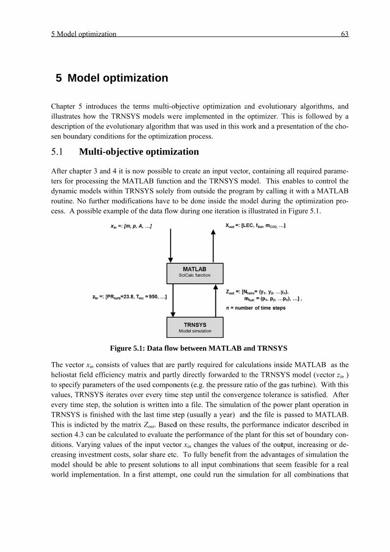
5 Mod
5 M
Chapteillustradescripsen bo
5.1
After cters fodynamroutinecess. A
The veheliostto specvaluesevery tTRNSYThis issectionditionscreasinmodel world
del optimizat
Model o
er 5 introduates how theption of the undary cond
Multi-
chapter 3 anor processingmic models we. No furtheA possible e
ector xin contat field efficify paramet, TRNSYS time step, thYS is finishs indicted byn 4.3 can be s. Varying vng investmen
should be aimplementa
tion
optimiz
uces the tere TRNSYS evolutionaryditions for th
objective
nd 4 it is nowg the MATLwithin TRNSer modificatiexample of t
Figure 5.1
nsists of valuciency matrters of the usiterates ovehe solution ihed with they the matrixcalculated t
values of thent costs, solable to presation. In a fi
zation
ms multi-obmodels wer
y algorithm he optimizat
e optimiz
w possible tLAB functioSYS solely ions have tohe data flow
1: Data flow
ues that are rix and partlsed componr every timeis written in
e last time stx Zout. Basedto evaluate te input vectolar share etcent solution
first attempt,
bjective optre implementhat was us
tion process
zation
to create an on and the Tfrom outsido be done inw during one
w between M
partly requily directly fonents (e.g. the step until nto a file. Thtep (usually
d on these rethe performaor xin chang
c. To fully bns to all inpu, one could
timization anted in the ed in this w.
input vectorTRNSYS mode the progranside the moe iteration is
MATLAB a
ired for calcorwarded to
he pressure rthe converghe simulatio
a year) anesults, the peance of the pes the valuebenefit fromut combinatrun the sim
and evolutiooptimizer. Tork and a pr
r, containingodel. This am by callinodel during illustrated i
and TRNSY
culations ins the TRNSYatio of the g
gence toleranon of the powd the file is erformance plant for thises of the out
m the advantaions that se
mulation for
onary algoriThis is folloresentation o
g all requireenables to c
ng it with a Mthe optimiz
in Figure 5.1
YS
side MATLAYS model (vgas turbine). nce is satisfiwer plant oppassed to Mindicator des set of bountput, increasages of simu
eem feasibleall combina
63
ithms, and owed by a of the cho-
ed parame-control the MATLAB zation pro-1.
AB as the vector zin ) With this
fied. After peration in MATLAB. escribed in ndary con-sing or de-ulation the
e for a real ations that

5 Mod
can beoverallble comvious tdifferepointleered as
If we cthis caobjectivariabl= (e1(xtemperin comobjectirepresecase. Tfunctiothe moobjecti
The cosolarizby the limitedwould purposfor thewill mminim
Theresatisfylems.
del optimizat
derived frol calculationmbinations wthat a solar
ent inputs seess model cos better ones
consider Figase minimizive functionles x = (x1, x), e2(x)…en
rature). The mbination wiive functionenting the bTo this valueon does not odel with onive function
Fi
onfigurationzation at all
savings of d solar sharebe the prefe
se of the powe search of th
most likely gemal chance of
fore, a secoying this add
The optima
tion
om the input n time wouldwill result infield of onl
eparately seonfigurations than others
gure 5.1, fore. It is then
n. The optimx2, …xn) (e.(x)) and a nset of decis
ith the constn searches fobest possiblee one specifnecessarily
ne objective n, resulting in
igure 5.2: E
n with the lobecause thefossil fuel.
e if operationferred solutiower plant – he maximumenerate the mf deploymen
nd criteria oditional objeal design is o
vector. Witd soon exceen a solutionly 50 mirroren may be
n. This means. Finding th
r instance thn called the
mization procg. the numb
number of csion variabletraints e(x) dor the globae system defic solar shahave to hav
as the minimn trivial solu
xpected opt
owest levelie additional
This comesn beyond theon from a puto generate
m solar sharmost expensnt.
or objective ective. Manyoften a com
th an increased reasonab
n that represers does not useful, theirns, in the se
hese solution
he LEC coulobjective, a
cess is charaber of heliosconstants c =es defines thdetermine thal optimum,esign; whichare is assignve a global mum LEC, iutions, see F
tima in a si
ized electricinvestment s from the fe hours of sourely economelectric pow
re. If this pasive plant co
must be esty real world
mbination of
sing amountle timeframents a realizneed a towr combinatiet of possiblns is the goa
ld be the vaand the equaacterized bytats or size)= (c1, c2, …he decision she set of fea
returning ah would beed. As illustminimum oit is possibleFigure 5.2.
ngle objecti
c cost mightform a sola
fact that the olar insolatiomic point of
wer partly foarameter is configuration
tablished to d problems two or more
t of elementses. In additi
zable model.er of 200m on in one vle solutions,l of an optim
ariable we wation that dea set of n p
, constraintscn) (e.g. thespace x = (xsible solutio
a single pointhe lowest
trated in Figor maximume that the sam
ive optimiza
t always ber field mighpower planton is desiredf view, it faiorm solar enchosen as th
n possible, w
obtain the oare usually e competing
s within the ion, far from. It is for exin height. W
vector may r, some can bmization alg
want to optimefines the L
parameters os to this varie fixed recex1, x2, …xnons. Out of tnt in the seaLEC possib
gure 5.2, them. If we onlyme will happ
ation
e the one wht not be comts can only d. While this
ails to includnergy. The she objective,which will h
optimal solumulti objec
g objectives,
64
vector the m all possi-xample ob-While two result in a be consid-orithm.
mize, or in LEC is the or decision iables e(x) iver outlet
n) ∈ X and this set the arch space ble in this e objective y optimize pen to this
ithout any mpensated generate a s optimum
de the very ame holds , the result ave only a
ution while ctive prob-, as for in-

5 Mod
stance solar sconducglobal tationadecisiomizatiomulti-ooptimi
Whennative space istrongltion x2
to all o
⊢
This nfoundaPareto
del optimizat
lowest costshares. If thected, by varyfield of equ
al times dueon about whon that charobjective opized, each re
n two or mortrade-offs.
is superior tly based on
2 (x1 ⊢ x2) ifother objecti
⊢ ⟺ ∀ :
otation is alations to muoptimal. He
Figure 5
tion
ts at the highe optimized ying the var
ually good soe to many ruhich system racterizes alptimization. epresenting o
re competinEach soluti
to it when althe definitio
f x1 is better ives. For the
: 0
so called Paulti-objectiveence, the Par
5.3: Illustra
hest performLEC for a d
riable’s consolutions canuns and canto choose hl of the inteInstead of o
one objectiv
: →
ng objectiveson is optimll objectiveson of dominthan x2 in at
e set F of ob
⇒
areto dominae optimizatioreto optimal
∗ ∈ ∗ ⟺
ation of a ge
mance possibdifferent solastraints. Givn emerge. Thnnot guaranthas to be takeresting regione objectivve.
: 0 ,
s are selectemal in a wides are considenation. A soat least one objective func
∧
ation, after Von. Solutionl front X* co
⟺ ∄ ∈ :
eneral multi
ble, or in thear share is w
ven a sufficiehis however tee to find a
ken, the decions of the m
ve function f
⊆
ed to be optier sense thaered. The no
olution x1 doobjective functions fi it ca
∃ : 0
Vilfredo Parns that are nonsist of the
⊢ ∗
i-objective o
ese models lwanted, paraent amount ocomes at th
all solutionsision maker model. This f, a set F of
imized, the rat no other sotation of opominates or nction and nan be written
:
reto (1848-1ot dominatenon-domina
optimizatio
lowest LEC ameter studieof optimizat
he cost of lons of interestwould prefecan be achiobjective fu
result is a sesolution in ptimal in thiis preferred
not worse wn:
923) [51]whed by others ated solution
on problem
65
at highest es must be tion runs a ng compu-. When a
fer an opti-ieved with unctions is
(5.1)
et of alter-the search is sense is
d to a solu-ith respect
(5.2)
ho laid the are called
ns x*.
(5.3)

5 Model optimization 66
Figure 5.3 illustrates some of the discussed issues. With the set F of objective functions, possible solutions are calculated in the objective space. Assuming a minimization problem, the best solu-tions are those closest to the Pareto optimal front. All shaded solutions dominated the filled ones. For example, comparing the solution B and C, it is found ∧ . Solu-tion B therefore fully dominates solution C. This however is not the case when comparing the solutions B and A. Each solution dominates the other in one objective, but not in the other. Both solutions are part of the Pareto optimal front. While all solutions within the objective space satis-fy the constraints given to the model, only those solutions situated on this front can be considered as optimal. In contrast to single-objective optimization, where a solution can only be better or worse - ∨ - a third option ≱ ∧ ≱ exits for multi-objective problems.
With MOO, fewer assumptions have to be made before optimizing and provide the decision mak-er with a range of solutions to choose from. This is often important because an optimization prob-lem is a simplification of a real world problem that in part can require human or unquantifiable judgment. For example, the land consumption for large scale CSP is considerable and combined with high towers might encounter serve resistance in the population, making the deployment over a certain size impossible. In these types of problems, an optimizer needs to suggest various possi-ble alternatives that can later be judged. Additionally, with several objectives a better understand-ing of a search space can be achieved in terms of the location of its various optima.
Several multi-objective optimizers are available. To select the one that fits best requires infor-mation about the structure of the system that is supposed to be optimized. The influence that the optimizer can have on the model is limited. As stated in Chapter 3 the TRNSYS simulation can be considered as a black box. A set of parameters are presented as inputs and the black box gives a number of outputs. Derivatives of the outputs with respect to the inputs and any extra information about the form of the model are not available. Moreover, a modification of the individual compo-nents is not easily possible, because that would require a recompilation of the source code they are written in. Furthermore, the optimization tool must be able to handle non-linearities, and discon-tinuous and/or disjoint models. These situations can for example easily occur due to rapid chang-es in insolation values or part time operation of the plant.
If conventional techniques are applied, they will usually work according to the principle “Deci-sion making before search”. The objectives of the multi objective problem (MOP) are aggregated into a single objective , resulting in one optimization criterion; very much like a classic single-objective technique but with the difference that the parameters of this function are not set by the Decision maker, but systematically varied by the optimizer [52] . This method makes these ap-proaches popular and widely used because well-studied algorithms for single objective prob-lems(SOP) can be applied.
However, several difficulties and drawbacks may accompany classical optimization strategies.
Conventional methods are based on assumptions of some level of continuity [53]
In order to merge several objectives in one optimization criterion problem knowledge may
be required which may not be available [52]

5 Model optimization 67
As in a SOP, several optimization runs have to be performed to obtain an optimal surface
Because the runs are performed independently from each other, synergies can usually not
be exploited which can significantly increase computing time.
Recently, evolutionary algorithms have become established as an alternative to classical methods through which i) large search spaces can be handled and ii) multiple alternative trade-offs can be generated in a single optimization run. Furthermore, they can be implemented in a way such that the above difficulties are avoided.

5 Mod
5.2
5.2.1
Evoluting therepresepredefas weldiffereThese crossovthem tsearch qualityindivid
Figure
del optimizat
Evolut
Overvie
tionary algoe evolutionaents the set ofined schemell as in the oent operators
operators cver/combinato a one or
space whily is judged oduals decide
e 5.4: Gener
tion
tionary a
w
rithms (EAsary cycle. Fiof solution ce. The indivobjective sps individualan either beation, whichmore childrle increasingon the so cales about the p
ral data flo
algorithm
s) model thegure 5.4 depcandidates c
viduals contaace when ths of low qu
e mutation wh create a neren. Therefog its averaglled fitness oprobability t
ow in an EA
ms
e biologic prpicts a simpcalled indiviain informathe objective uality are remwhich alter sew individu
ore, the popuge quality. Wof each indithey are rem
Whileassignhave often the fithe pportanquickin a derivoptima conzationtionalpredetermithe exity caapplicentireproxidefinobjec
A
rocesses of sple applicatioiduals. It is etion about th
function is moved and small parts
ual by selectulation evolWhich partsividual. The
moved from t
e it might sn those inda high qualdesirable to
itness assignpopulation cnt to avoid
kly to a too slocal, non-gative-free, t
mal set only wnvergence ern process cal criteria muefined maximnation criterxistence of aan be used.cations the e Pareto-optmation. Based the goals
ctives:
survival of ton scheme. either createheir position
applied. Wones of higof already eting two parves to the o
s of the popway the fitnthe set.
eem obviouividuals witlity objectivo include otnment. This can be mainthat the alg
small regionglobal, optimthat is they with the objrror limit to annot be appust be intromum numberion, but alsan individua In any cassolution wil
timal set, bused on this bs for an EA
the fittest, imThe initial p
ed at randomn in the deci
With the use gh quality reexistent indirents an recoptimal regipulation are ness is assig
us in the firsth a high fi
ve function vther charactway, the d
ntained whigorithm convn, and thus gma. Because
calculate thective functterminate th
plied. Thereoduced. Verer of iteratiso other conal with sufficse, for manyll most likeut a close ebehavior, Zin three mo
68
mplement-population
m or after a sion space of a set of eproduced. ividuals or combining ons of the of higher
gned to the
st place to fitness that value, it is teristics to iversity of ich is im-verges too
get trapped e EAs are he Pareto-tion values he optimi-efore addi-ry often, a ions is the nditions as cient qual-y complex ely not the nough ap-
Zitzler [52] ore general

5 Mod
Fig
Havinggives aschem
In ordeknow wtor, thetowardor. Onsolutiobe closto eithpossibabove,incorpfitnessistics r
Once eselectioperatodeterm
del optimizat
The distanminimizedfairly wideoptimal fro
gure 5.5: Sol
A good disfront shou
The spreadtive a widegive the delutions not
g establishean overviewe of the algo
er to move which solute so-called fds the POF, ly when the
ons inside thser to the PO
her X1 or X2
le solution b, to avoid a orates apart
s value assigrelative to th
each solutioon operationors are appl
ministic – the
tion
nce of the red. This is dee spread in ont should b
lutions at th
stribution ofld be able to
d of the obtae range of vecision makt only locally
d this roughw of some iorithm used
the populatiions can be fitness is nethe comparisolutions ar
he objective OF and no p
2 exists elsebecomes tota
fast convert form the qgned may nohe whole pop
on (or indivins to chooselied to genee best indi
esulting nonepicted in Fthe objectiv
be clearly ide
he start of t
f the solutioo be approxi
ained nondovalues shouler a wide rany but in all r
h overview important ein this work
ion towardsselected foreded, ratingison must alre considerespace are corogress tow
ewhere. Withally orderedrgence towaquality of itsot only depepulation.
idual) of thee which indierate individividuals of th
ndominated igure 5.5. A
ve space. Onentifiable.
the optimiza
ons found is imated with
ominated frold be covereange of alternregions of th
of how an Elements of
k can be exp
s the Pareto r reproducti
g a solution lso report th
ed to lay on tonsidered eq
wards the opth the assign
d, creating a ards a singles objective vend on the so
e populationividuals makduals for thhe populatio
front to theAt an early nce the sim
ation(left) a
desirable. Ia fitting fun
ont should bed by the nonnatives, the he search spa
EA is suppoan EA. Wi
ploited.
optimal froon and whicX1 superior
hat the true sthe POF theyqual, there istimum can bned fitness vfitness land
e local optimvalues additolution cand
n has an asske it into the
he next geneon are used f
e Pareto-opoptimizationulation is te
and after ter
In a good opnction.
e maximizedndominated algorithm shace.
osed to worth this back
ont (POF), thch not. Theto X2 or vic
superior soluy should be s no informa
be made unlevalue to eacscape of themum, the fittional informdidate itself
signed fitnese mating pooeration. Selefor the popu
ptimal front n stage, solerminated, th
rmination (
ptimization
d, i.e., for ead solutions. Ihould find o
rk, the next kground, th
he algorithmerefore, a clece versa. Foution is inderated as equation as to wess a superioch solution, e populationtness valuesmation. Therbut also on
ss value, thol. Here, repection can bulation at the
69
should be lutions are he Pareto-
(right)
result, the
ach objec-In order to optimal so-
paragraph e working
m needs to ear indica-or progress eed superi-uivalent. If which may or solution the set of
. As stated s normally refore, the character-
e EA uses production be entirely e next iter-

5 Mod
ation. Osplit theach inequivainto thmade bone itenumbereplacemove ttained,tion, acby havmovedin steafour ex
Havingstep isreprod
The baindividand cotion usstates, tion onassigneinteres
As illuations of howthat leathe algtics.
5.3
The optems Lsystem
del optimizat
Or it can ushem in thosndividual caalent in the mhe mating poby the genereration to aner of childree the existinthe populati, but a few octing as a mving more cd, and indiviady-state EAxamples of d
g analyzed s to create tduction proce
asic conceptduals that is ombination. ses the inforthat combin
nly occurs wed with a disting.
ustrated in Fcreated a sa
w to performad to the PO
gorithm that
The Q
ptimizer useLaboratory), m problems a
tion
se a stochaste with repla
an contributemating poolool several trational stru
nother. In geen equal to ng populatioion toward aof the very b
marker of thechildren. In iduals are re
As result in sdifferent sele
which indivthe new geness.
t behind thesimilar to thMutation airmation encnation is usuwith a low pfferent prob
igure 5.4, thatisfying PO
m an optimizOF are far fr
was used in
ueueing
ed for the mat the Univ
and has been
tic selection acement and e to reprodu. Selection stimes, creatiucture of theenerational Ethe size of
on. This mean optimumbest individue best perforsteady-stateplaced whensome measuection schem
viduals shouneration by
e operators he existing pims to makecoded in twoually used onprobability. bability, driv
he optimizatiOF. Apart frozation basedrom completn this work.
Multi-Ob
models in thiversity of Lan tested on a
strategy. Od such withouuction proceschemes witing a numbee algorithm tEAs, the popthe populat
ethod relies m. In elitist Euals in the pormance of the EAs, the gn necessary.ure of elitismmes are give
uld be choseapplying a
imitating repopulation.
e small chano individualn every newDifferent m
ving the new
ion can nowom the men
d on an evolute. HoweverThe next se
bjective O
is work wasausanne. It wa number of
ne way to dut replacem
ess not moreth replacemeer of offsprithat is how pulation is ption is generentirely on
EAs, the genopulation ar
he algorithmgenerational. Very oftenm. In the folen.
en to be copvariation of
eproduction The two op
nges to a sinls to combin
w individual mutation opew population
w be terminationed schemutionary algr, the here dection will n
Optimize
developed was specificaf test proble
distinguish seent. Withou
e than once, ent can placing. Anotherthe populatirocessed a grated, and ththe selectio
neration strure kept from, and contrib structure o
n the criteria llowing, sim
pied to the mf operators t
is to createperators usedgle individune it to a nein a new ge
erators can bs in one cert
ated, if a suffme, many mgorithm. Alsdescribed waow briefly e
er
by LENI (Inally develop
ems [53], wh
election schut replacemethus having
ce the same r classificatiion size chageneration ahese childreon of good ucture is gen
m generation buting to co
of the algoria for removamplified desc
mating poolthat mimic
e a new gend for this areual, whereasew one. Leyeneration, wbe implemertain region t
fficient numbmore possibiso, the preseay helps to uexplain its ch
Industrial Enped for solvihere it proof
70
hemes is to ent means, g only one individual ion can be
anges form at a time: a en entirely parents to nerally re-to genera-
onvergence ithm is re-al of points cription of
l, the next biological
neration of e mutation s combina-yland [53]
while muta-nted, each that seems
ber of iter-lities exist
ented steps understand haracteris-
nergy Sys-ing energy fed to be a

5 Model optimization 71
fast converging, and robust optimizer that is able to find local optima. Comparisons of the per-formance of the Queueing Multi-Objective Optimizer (QMOO) with other algorithms showed, that even in the worst case it performs only slightly poorer than others, whereas in the best case it is able to outperform all other algorithms. While using many of the above mentioned methods, it differs from other EAs in the way they are implemented. The most important modifications are explained in the following.
One major difference to other EA is the queueing structure of the optimizer. This property was implemented to allow the algorithm performing objective function evaluations in parallel. In an EA, where the evaluation is based solely on the objective function and no further gradient infor-mation, evaluation can easily be distributed to several processors or computers. The “classic” or also called synchronous approach would be to split the population into groups equal to the number of available processors. There, the individuals are evaluated and then send back to the main pro-cess to continue with the usual steps. Leyland describes this as one of the major advantages of EA. He notes that, although an EA is likely to need many more iterations to solve an optimization problem compared to more analytic methods, the overall computing time until the solution is reached is smaller.
The queueing process stocks the individuals once they received their decision variable values in a queue. From the queue, any processor can pick it and perform the evaluation. After the evaluation, the individual is returned, rated, and marked as a “full member” of the population, ready for serv-ing as a parent for a new individual. With this structure implemented, the algorithm cannot be described anymore in the strict ordered sequences as it was illustrated in Figure 5.4. All steps can happen at the same time as long as the queue contains individuals. Therefore, Leyland describes the algorithm with thestepsoneindividualgoesthroughfrom“birth”to“death”.Thesestepsare:
Creation: The individual is created with initial values and stored in the “assign” queue.
Assignment: The individual is taken from the queue and parameter values are assigned.
This can happen at random at the first iteration or by the reproduction operators for all fur-
ther iterations. The individual is then stored in the “evaluate” queue.
Evaluation: The objective function evaluates the individual and passes it to the “grouping”
storage.
Grouping: The individual is assigned to a group and stores in the “ranking (fitness as-
signment)” group.
Ranking: A fitness value is assigned to the individual and from here on available for re-
production processes.
Removal: If the individuals fitness is lower than a limit set by appropriate processes, it
will be removed from the population

5 Model optimization 72
This lifecycle includes the method grouping, which has not been explained yet. Its task is to main-tain a certain diversity of the population by forming several groups out of the population. Individ-uals of different groups cannot compete against each other, but a certain level of interbreeding is allowed. Grouping can be time-consuming and is most beneficial when the POF is disjoint or more than one POF exists. For the problems in this work, experience with similar models shows that the solutions will consist of only one POF, which is why this element was not used in the optimization process.
In the removal step, “appropriate processes” are mentioned to decide about the preservation of the individual. Which processes are used depends much on the generational structure of the EA. As mentioned in section Error! Reference source not found., a generational algorithm replaces the entire population with new individuals at each iteration. This way, all individuals cannot prevail longer than one generation in the population. In a steady-state EA however, this is not the case. In fact, the creation of new points and the removal are two separate processes. Choosing two parents to create a child has no direct consequences for the parents and will temporarily increase the population size. Individuals are only removed when they are found to be lacking in some way. In QMMO, the ranking process also includes a method to remove individuals. This happens in two ways: If an individual has exactly the same objective function values as another individual, it is removed from the population. For the remaining individuals, the process uses a variation of the Pareto ranking (section Error! Reference source not found.), removing elements after the fol-lowing scheme:
“The ranker should rank members of the population at least up to rmin, and ensure that at least Gmin individuals have been ranked. Past these limits, the ranking should give individuals a rank of −1, indicating that they are so poor they should be removed from the population. [53]”
This method works well as long as the algorithm has not produced a well distinctive POF, and rmin
has a relatively low value. However, with increasing iterations rmin will increase to maintain se-lective pressure. At some point rmin will reach the maximum value that can be assigned to an indi-vidual and the group analyzed will consist of non-dominated individuals only. If now further re-moval of individuals is desired (because the solutions so far a not sufficiently distributed), a method is needed to remove non-dominated individuals. This is achieved by introducing thinning methods. The individuals to be removed are chosen based on their location in the objective space relative to the rest of the group. The best individuals to remove are those that offer little more information about the form of the POF (effectively, those that are in a crowded region in the non-dominated set), and individuals that are far from the POF. Implementing this method not only maintains the selection pressure, but also avoids that the population can grow uncontrolled.
With the analysis of the main difference of the QMMO to conventional approach, the main fea-tures of the algorithm can be summarized.
QMOO is a steady-state EA. Individuals are only removed from the population when their parameters are considered to be of some sort of low quality.

5 Model optimization 73
QMOO is an elitist EA. However, no external set is used. Instead, the population only contains the best solutions found so far. Methods like grouping are implemented to coun-teract the problems of diversity preservation induced by elitism.
QMOO performs grouping or clustering. QMOO preserves diversity by dividing the popu-lation into groups and letting these groups evolve independently. Grouping using cluster-ing methods from statistical analysis proved to work very well.
QMOO implements Pareto-based multi-objective optimization. Individuals are ranked in order to identify individuals that approach best the Pareto optimal front. The method used is based on Pareto ranking.
QMOO has a queue-based design. Individuals are viewed as independent entities that must go through a number of processes (creation, evaluation, ranking, grouping) in order to join the ‘main population’. It makes the algorithm easy to parallelize and efficient when running in parallel.
QMOO implements the Evolutionary Operator Choice (EOC). This means that the choice which operator is used for reproduction is left to the algorithm. A successful children (one that remains in the population) should try to use the same operator for its offspring.
The QMOO is a toolbox provided in MATLAB. It uses another platform, called OSMOSE ('Op-timiSation Multi-Objectifs de Systemes Energetiques integres'), which was also developed at the University of Lausanne. OSMOSE is a unifying tool, designed to integrate different models for the analysis of integrated energy systems. One of this models is the here described multi-objective optimizer. In the next section, the interaction and the required modifications of OSMOSE and MOO are described, and the data flow analyzed. This is followed by the presentation of the pa-rameter decisions made for the optimization.

5 Mod
5.4
5.4.1
Neitheprocesoverviin Figu
Of couever, nwhereamose_lem. sothe TRelemenwith thdefinit
del optimizat
The op
Program
er OSMOSEss in enteredew of the daure 5.1
Figure
urse, OSMOno explicit inas the three
_interface areolCal is the RNSYS simnts symbolizhe program stions require
tion
ptimizatio
m descriptio
E nor MOO d in the accata flow. Th
5.6: Simpli
OSE and MOnteraction o depicted fue provided bfunction tha
mulation. Thize the outpustarts with thed for the o
on setup
on
have a grapcording MAhe two lowes
fied data flo
OO themself or modificatiunctions muby the optimat calculates is function ut that is crhe function fptimization
phical interfaATLAB func
st elements r
ow scheme
f consist of aion by the uust be create
mizer packagthe plant’s phas been dereated durinfrontend_sois entered.
ace. That mctions directrepresent th
during the
a large numbuser is requied or modifge and have performanceescribed in
ng the optimolarPlant. H
The user ca
eans that alltly. Figure 5e scheme th
optimizatio
ber of MATired. In ordefied. frontento be adaptee and costs, Chapter 4.
mization proere, all necean choose b
l data requir5.6 gives a hat has been
on process
TLAB functier to run thend_solarPlaned to the curusing the reThe diamo
ocess. Commessary informbetween a va
74
red for the simplified illustrated
ons. How-e program, nt and os-rrent prob-esults from nd shaped
munication mation and ariation of

5 Model optimization 75
different operation modes, for example if the program should run only once, if a multi-objective optimization or a sensitivity analysis is desired or if an interrupted calculation process should be resumed. Following this, the initial population size and the number of clusters has to be specified. A value for initial population that seemed to give sufficient diversity and kept the calculation times low was 100 . As mentioned in the previous section, clustering or grouping was considered to have no additional benefit on the solution quality and was therefore left to a value of one. These configurations are independent of the type of the power plant being optimized. This is not the case for the following definitions of the plant variables. These include the objectives of the opti-mization, the variables, their limits and the constants. Once all required parameters are set, the function passes them to OMSOSE, where they processed to a readable structure for MOO. As illustrated, communication between OSMOSE and MOO is handled internally, no adaption by the user is necessary. MOO then selects values for the variables of the first generation. The function osmose_interface is required to prepare the data for the processing in the actual plant simulation. It reads the number of objectives, variables and constants from OSMOSE and creates an input vector of theses parameters containing the initial values from MOO. osmose_interface then calls the function solCalc that controls TRNSYS and does the performance calculations after TRNSYS has finished its run. solCalc passes all performance parameters described in section 4.3 back to osmose_interface. Now, two performance parameters are selected and assigned as the objectives for the optimization. All calculated parameters from solCalc are coupled with current values of the input parameters that define this plant configuration and stored with the function write_result. The objectes are passed on to MOO where the optimization starts after 100 points have been cre-ated. While with write_result the results from every run are stored, the population size of MOO cannot exceed 100, which is why the optimizer only knows of the 100 current results. Without the implementation of write_result only the best 100 results can be used. While they are most likely in a satisfying distance to the POF, the density of the solutions is low. By storing every run, sev-eral hundred optimal points can be plotted by checking the two objectives of the result file for Pareto dominance, eliminating all iteration results that are dominated by one of the two objectives. An output created by OSMOSE is labeled run_number. ‘number’ refers to the current optimiza-tion run. All data required to rerun an optimization after an interruption is stored there.
5.4.2 Parameters chosen for the optimization
As mentioned above, three types of input parameter have to be selected:
Objectives
Variables
Constants
As objectives two competing parameters must be chosen. After some test runs, the solar share and the investment costs were selected. Using the LEC gave an unsatisfying Pareto front. The reason will be explained later in this section.
The plants are designed to operate with a constant power output, using a one specific power unit. Therefore, varying values within the power cycle are not wanted. The goal is to equip the cycle

5 Model optimization 76
with a solarization preheating system of different power sizes and operating times. This is achieved by varying the size of the solar field and the receiver. The chosen variables and their ranges are shown in Table 5.1. The ranges limits are chosen by common sense, tested, and adjust-ed if necessary.
Variable Range
SGT750 SGT400
Number of Heliostat Cells 5 – 250 [ - ] 5 – 150 [ - ]
Receiver Surface Area 1 – 300 [ m2 ] 1 – 150 [ m2 ]
Heliostat Surface Area 10 – 250 [ m2 ] 10 – 150 [ m2 ]
Tower Height 50 – 350 [ m ] 50 – 200 [ m ]
Table 5.1: Selected variables and ranges
An indicator that the range should be extended is when a crowded region of solutions at one limit occurs. For the SGT400 smaller ranges were selected. This is partly because of less solar power being required than in the SGT750 and partly because of problems with the TRNSYS model that will be described later. The selected ranges gave good results and were used for the hybrid cycle and the combined cycle. Several additional values were included, here labeled as constants. This means that they were not altered once an optimization run was stated. However, their values can be changed from one run to another. For a complete overview of the selected constants see Table A. 5 in the appendix.
For the combined cycle some additional values had to be defined. Beside the variables mentioned above, the optimizer could pick the pressure ratios for the steam turbine stages, with a deviation of 20% from 100bar, 20bar and 4bar. The values for the cooling water were included, but left un-changed. For the heat exchangers the same efficiency was assumed.
Variable Range
Pressure ratio SGT750/400
Stage one 120 – 80 [ - ]
Stage two 16 – 24 [ - ]
Stage three 3.2 – 4.8 [ - ]
Table 5.2: Variables for the combined cycle
Constant Value
Pressure ratio SGT750/400
Temperature cooling water 20
∆ cooling water 10
Heat exchanger efficiency 0.85
Table 5.3: Constants for the combined cycle

6 Resu
6 R
Four dplant, titerationecessby comall of tanalyzfrom th
6.1
Beforeof the
Figuretributebines a
ult of the opt
Result o
different contotaling in eons, followinsary. Apart fmbining conthose correlazed individuhe literature
Evalua
e a detailed solutions are
e 6.1 shows ted POF. Thisand load con
timization
of the o
nfigurationseight optimizng a check from the tw
nflicting elemations of par
ually and thee. Additional
ation of a
performance illustrated
the progresss shape of thnditions.
Figur
optimiz
(two gas tzation runs. of the POF o objectives
ments from trameters thaen comparelly, the impa
a multi-ob
e analysis othat apply f
sion of the Lhe POF is re
re 6.1: Typic
zation
turbines, twEach optimand an addi
s, a number the result filat can help td with otheact of varyin
bjective
of the differfor all config
LEC for increpresentativ
cal POF for
wo load condmization was
itional run tof different
le. The intento outline treer configurang fuel costs
optimiza
ent cases is gurations.
reasing solare for all pow
r the analyz
ditions) wer allowed to
time of 1000t correlationntion for thiends and cotions, as weand heliosta
ation resu
conducted,
r share in a wer plant co
zed cases
re simulatedperform at
0 or more itns can be inis chapter is onclusions. Rell as with at prices is p
ult
some chara
smooth andonfigurations
77
d for each least 1000
terations if nvestigated
to present Results are references presented.
acteristics
d well dis-s, gas tur-

6 Resu
As it cLEC foin the Cfuel fotion fahigher both efalmost
A lineaUp to tshares to drop
The so
ult of the opt
can be seenfor around thfactors that
or higher solactor, the inv
solar sharesffects for sot constant LE
ar increase othis point thof over 20%
p linear.
olar share is
The plant maintains the usable The limit c
The gas tuclosed with
timization
, an increashe 0 – 20% scontribute t
lar shares havestment coss. With the v
olar shares toEC. This eff
of the dottedhe increased % the dotted
limited for t
operates nothe constanhours of da
can be incre
urbine inlet th supplemen
ing solar shsolar share. to the costsave a positivsts and the cvalues seleco 20% havefect is illustr
Figure 6.2
d curve can bcosts can b
d curve begi
two main rea
ot only durinnt power outaylight and aased with pa
temperature nted firing w
hare (a largeThis effect (see equatio
ve influence costs for opected to detere the approxrated in Figu
2: Breakup
be observedbe covered bins to rise ex
asons:
ng hours of tput. The madditional mart load oper
cannot be rwhich negati
er solar fieldcan be expla
on (4.33)). Won the LEC
eration and mrmine the deimately sam
ure 6.2.
p of the LEC
d until a solaby increasingxponentially
solar insolamaximum achmetrological ration, as it w
reached by sively impact
d) has virtuaained with a
While the red, the combinmaintenancepreciation fa
me absolute v
C
ar share of arg fuel savingy, while the
ation. In thehievable solinfluences
will be show
solar preheatts the solar s
ally no impa break-up oduced fuel mnation of thee increase thfactor, the grvalues, resu
round 20% igs. Howeverfuel saving
ese periods, lar share is such as ove
wn in later.
ating. The gashare.
78
pact on the of the LEC mass costs e deprecia-he LEC for radients of lting in an
is reached. r, for solar
gs continue
fossil fuel limited by
erclouding.
ap must be

6 Resu
The strtures a
(a)
(c)
The grday. Terate aAt all
enough
closed
deflect
,
ment, tit can ptrates a
ult of the opt
rong increasand the shape
Full loa solar
Full loa solar
Figure
raphs in FigThe shaded (bat full load c
other times
h. In all illu
by ,
ted by the so is reached
the receiver provide cana solar field
timization
se in LEC fe of the dail
oad hours tfu
r field of the
oad hours tfu
r field of the
6.3: Progre
gure 6.3 illublue) area re
conditions. Ts , is
ustrated case
and the cu
olar field. Ifd only once
would opern eventually d that is large
for solar shay DNI curve
ull for a plante size
ull for a plante size 3
ession of th
ustrate the inepresents thThis means ts not reache
s ,
urve the sola
f this is to be, namely wh
rate always bbe used. Ase enough so
ares over 25e. Figure 6.3
t with (
t with (
e solar shar
nsolation a phe hours of tthe receivered because
is reached
ar power to
be avoided, then the DN
below its pos a result theo that the rec
5% is due to3 depicts the
b) Full solar
(d) Fullsola
re with incr
plant of a cethe day durinr operates atthe concent
before the D
high for th
the solar fieI peaks. Ho
ossibilities –e solar shareceiver can o
o limited rece correlation
load hours r field of the
l load hours ar field of the
reasing sola
ertain size cng which thits maximu
trated solar
DNI peaks.
he receiver u
ld must be awever, expe
only a fracte will be lowperate for
ceiver outlen of this two
tfull for a ple size 2
s tfull for a plhe size 4
ar field size
can collect dhe power plaum outlet tem
radiation is
In the empt
und therefor
adjusted in ect for this s
tion of the sow. Figure 6
hours a
79
t tempera-factors.
ant with a
lant with a
during one ant can op-mperature. s not high
ty area en-
re must be
a way that single mo-
olar power .3(a) illus-day at de-

6 Resu
sign po6.3(b)
reachehours tributin
tion (bthe solmovindoublincurve. tempershare i
Origingave ashares.with tha resulGroupcosts afor smas it w
All solkept in
6.2
The forun co
ult of the opt
oint. Nevertshows the
ed earlier anavailable in
ng to a large
b) further imlar share incg from (c) fng of the soThe only w
ratures. As is coupled w
nally, besidea poor distrib. If two solhe lower sollt, the POF ing can proare selected
mall solar shawas the case f
Fig
lutions on thn the populat
Result
ollowing chanfigurations
timization
theless, morbehavior of
nd can be mn configuratier , and
mproves the fcrease is mufor (d) with olar field, thway to overclong as only
with an expon
the solar shbution of thelutions in Filar share is dmight lack
obably overcas the seco
ares since thfor the LEC
gure 6.4: C
he POF in thtion.
s for the
arts show ths. Figure 6.6
e than 50% f the same r
maintained loion (a). The therefore a h
full load/paruch smaller t
even less ahe increase income this fay one receivnential rise o
hare, the LEe POF. The igure 6.1 hadominated bsolutions fo
come this efnd objective
hey are not a. The differe
omparison
he left graph
hybrid c
he results fro6 displays th
of the day, receiver for
onger. The square left higher solar
rt load ratio,than it was additional gain solar sharact is to impver is availaof the LEC.
EC were selreason for th
ave the sameby the other or low solarffect, howeve. This is beaffected by ence of the i
of the initia
h of Figure 6
cycle
om the hybrhe solar shar
the receiverr a larger so
inner dasheand right to
r share. Dou
, as it can bein the first dain. Therefore decreases plement a reable, approa
ected as thehat is the stae LEC but dand can be
r shares whiver, it can because the ithe cost redinitial gradie
al gradient
6.4 are clear
rid cycle andre over the L
r is in part lolar field. A
ed square reit visualize
ubling the so
e seen in Figdoubling. Thore it can be
because of eceiver that ching the m
e second objagnation of tdifferent solaremoved froich would bbe also avoinvestment cuction causeents is depic
of Cinv and
rly non-dom
d the compaLEC for the
load operatiAs a result
epresents thethe gained h
olar field of
gure 6.3(c). he same appe said, that wf the shape o
can withstamaximal pos
jective. Howthe LEC forar shares, thom the popube interestinided if the icosts rise noed by the fu
cted in Figur
LEC
minated, and
arison of thee SGT400,
80
on. Figure
, is
e full load hours con-configura-
However, plies when with every of the DNI and higher sible solar
wever, this r low solar he solution ulation. As ng to have. investment otably also uel savings re 6.4.
therefore
e different Figure 6.5

6 Resu
the samwhen oUSc/kW
ult of the opt
me parameteoperating inWh and betw
timization
ers for the SGn base load aween 0.2 – 0
GT750. For and to 40% 0-3 USc/kW
Figure 6.5
Figure 6.
r both turbinin part load
Wh for the SG
5: Solar sh
.6: Solar sh
es, the solard. Using theGT400 for so
hare vs. LEC
are vs. LEC
r shares are le SGT750 Lolar shares u
C
C
limited to arLEC varies aunder 20%.
81
round 28% around 0.5

6 Result of the optimization 82
Despite the higher the fuel consumption, a base load operation is more cost effective than part load for small solar shares since it generates more energy. However, when the base load configu-ration approaches the maximal solar share, the costs are quickly surpassing the level of the part load configuration at the same solar share. Compared to Figure 6.1 the LEC are cut at 10 USc/kWh to reveal more details of the curve progression for lower solar shares and remove LEC that are too high to be considered as an interesting solutions. In Figure 6.6 it can be observed that at very low solar shares, the LEC initially drop slightly before gradually increasing. This charac-teristic is imposed by slight variations in the power output. Although the combustion chamber keeps the turbine inlet temperature steady it cannot influence pressure drop variations due to changing receiver sizes. At very low solar shares, the receiver size will be very small as well. However, the air mass flow passing through it remains the same, increasing the pressure drop compared to larger receiver sizes. To give examples of the parameter performance of the plants at certain solar shares and costs, two solar shares were selected, one for each load condition. In the interest of high solar shares coupled with low LEC, interesting solutions are for example a 25% solar share for the base load and 35% for the part load configuration. It must be mentioned that these values do not distinguish themselves in terms of higher solution quality from any other point on the POF. However, it is reasonable to assume that no decision maker will pick a solution with a lower solar share and almost equal cost, as it is certain that a plant deployment cannot be consid-ered as feasible if one or two percent point increase in solar share result in a doubling of the LEC. Therefore, these points should not be seen as the representative solutions of the optimization pro-cess, but rather as a landmark to make to some extent a comparison between the different possible cases. These values will serve throughout the evaluation as plant designs examples and for com-parison purposes. For the four curves, Table 6.1 gives approximate values.
SGT 750 base load
SGT 750 part load
SGT 400 base load
SGT 400 part load
Solar Share[%] 25 35 25 35
LEC [USc/kWh] 5.2 5.9 5.6 6.4
Spc. CO2 emissions [g/kWh] 327 290 351 310
Investment costs[MioUSD] 86 75 37 33
Receiver area [m2] 91 87 50 40
Number of heliostats 2790 1920 1102 766
Heliostat area [m2] 89 104 75 86
Total mirror area[m2] 250660 200520 82684 66153
Tower height [m] 128 117 70 64
Table 6.1: Analysis of two possible plant designs in hybrid configuration

6 Resu
The cothe fol6.9 illuence, tbase oric emising twsmalle
On ovconfigu
Fig
ult of the opt
orrelations bllowing paraustrate the Pthe specific r part load. Issions, as it o fixed LEC
er turbines an
erview overuration in ba
gure 6.8: Fr
timization
between solaameters in TPOF of the sCO2 emissiIn general, tdid for the c
C from the Snd part load
r the total enase load is ta
raction of th
0
0,2
0,4
0,6
0,8
1
%
Figu
ar share andable 6.1, the
specific CO2
ons can be the graphs shcosts in FiguSGT750 and
operation.
nergy generaken as a ref
he total energ
0
2
4
6
8
SGT 750base load
ure 6.7: spe
d the LEC we graphs fol
2 emissions.cut by arounhow that de
ure 6.5 and d SGT400. O
ration is giveference, wit
gy generatio
0d
SGT 750part load
ecific. CO2 e
were shown llow on the Taking thend 30% andcreasing theFigure 6.6.
Of course, th
en in Figureth 28
on , with SG
SGT 400base load
Sb
emissions vs
in Figure 6.next pages. se costs from
d 40% respee turbine sizeThis can be e total CO2
e 6.8. The o80GWh/a.
GT 750 base
SGT 400ase load
s. LEC
.5 and FigurFigure 6.7 am SGT750
ectively, depe increases tidentified bdischarge is
output of the
load as refe
83
re 6.6. For and Figure as a refer-
pending on the specif-
by compar-s lower for
e SGT 750
erence

6 Resu
A comsolar ssolar s
ult of the opt
mparison of share the cosshares the co
timization
Figu
the investmsts equal theosts for the
Figu
ure 6.9: spe
ment costs foe investmentfield, tower
ure 6.10: Sol
ecific. CO2 e
or different t necessary r and receiv
lar share vs
emissions vs
solar sharesfor the pow
ver are adde
s. Investmen
s. LEC
is given iner generatio
ed. As seen
nt costs
n Figure 6.1on unit. For
in Figure 6
84
0. At zero increasing
6.1, for the

6 Resu
chosenthe dif
The fothe optand onshares For theplant cif the ais apprreceivemirror plottedinclinathe SG
ult of the opt
n solar sharefferent turbin
ollowing foutimizer. In Fn the right h
over 25% ae SGT400 thconfigurationabove mentiroximately 7er area. A liarea is the
d against theation can be GT400 these
F
Fig
timization
es, the powene sizes.
ur graphs illuFigure 6.11 hand side ovand 35% reshis limit cann approacheioned target 70m. In Figuinear correlaproduct of t
e solar shareobserved. 1values can b
Figure 6.11:
gure 6.12: T
er plant inve
ustrate the gon the left hver the towespectively arn be found ates its solar svalues for thure 6.12 the ation exists bthe heliostate, an abrupt 100m2 are sube reached w
: Solar shar
Total mirror
estment cos
general trenhand side theer height. Fire only achit around 100share limit. The solar sha total mirrorbetween thet size and thtransmissio
ufficient for with less tha
re vs. helios
r area and s
ts differ rou
nd of variouse solar shareigure 6.11 revable with 0m2. The treTower heigh
are are desirer area and th
e total mirrorhe number oon from the
the SGT750an 50m2 of r
stat area an
solar share
ughly by a f
s parameterse is plotted oreveals that
mirror sizeend becomeshts of over 1ed. For the she solar sharr area and ref heliostats. linear gradi0 and the queceiver size
d tower hei
vs. receiver
factor of tw
s that were over the helfor the SGT
es smaller ths well-defin120m are unsmall turbinere are plotteeceiver size If the recei
ient to the exuoted solar se.
ight
r area
85
o between
defined in liostat area T750 solar han 150m2. ned as each nnecessary e, the limit ed over the . The total iver size is xponential shares. For

6 Resu
Compaoptimiable deence sthe resnot to equallythe rancompa
6.3
In the of the turbinescales.Figurelower When serveddiffere
In Figuthe caslower. two pla
Of couever, thFigure
ult of the opt
arisons withized plant coeviations in ource not fsults from thprovide hig
y attractive nge of possibared to anoth
Result
combined cgas turbine
e cycle is re. The solar se 6.13 and F
for moderacomparing
d that for a sence in costs
ure 6.14, it se for the hDifferent to
ant size curv
urse, the inithe initial gra
e 6.10. This i
timization
h results froonfiguration the results.
found. and Ehese optimizghly detailedsolutions in ble alternativher is neither
s for the
cycle, a steam. No furtherquired. Thershare over L
Figure 6.14. ate solar sha
the LEC ofspecific solas is to be exp
can be obsehybrid cycleo Figure 6.1ves exist.
tial investmadient of theis due to the
m literaturewith a numHowever, th
Error! Refezations. As d informatiothe graphs
ves. Therefor feasible no
combine
m turbine prr variation frefore, similLEC and spDespite add
ares. Howevf the same loar share, the pected.
erved that fo. Also, the 13, the SGT
ent capital re four cases e dampening
e are difficumber of small
he values foerence sourit was ment
on about oninto context
ore, a detaileor possible.
ed cycle
roduces addfor the solarlar curve precific CO2 editional costver, the effeoad conditio LEC match
or specific Cminimum re
T750 cases a
required is hare smaller
g effect of th
lt, because l differences
or LEC preserce not fountioned befor
ne possible st to other oped judgment
ditional electr preheatingogressions aemissions fots for the stect is more on but of dih. Therefore
CO2 emissioneachable spalways emit
higher, as it than it was
he additional
they usuallys that can acented in Tabnd. are in in re, the purposystem desigptions and tot over the qu
tricity from of the com
are to be expor the four ceam cycle, distinctive fferent turbi
e, from an L
ns the LEC ecific emissless CO2. N
is depicted seen for the
l energy prod
y present onccumulate toble 2.3, Erron good agreeose of thesegn, but to po give an ouualities of on
the hot exhmbustion air
pected but acases are diLEC are sigfor the largine size, it c
LEC point o
are lower tsions are sigNo intersect
in Figure 6e hybrid cycduction.
86
ne specific o consider-or! Refer-ement with e graphs is put several utlook over ne solution
haust gases in the gas
at different splayed in gnificantly ge turbine. can be ob-f view, no
han it was gnificantly tion of the
6.15. How-le cases in

6 Resu
ult of the opttimization
Figure
Figure 6.
6.14: specif
13: Solar sh
fic CO2 emi
hare vs. LE
issions vs. S
C
Solar share
87

6 Resu
The inexplaintherefoaround
44MW
ult of the opt
ncreased enened in chapore the addid 25% to the
We for the SG
0
0
0
0
0
0
0
0
0
%
timization
Figu
ergy generatpter 4, the gitional powee total energy
GT 750 and t
Figure 6percent
0
,1
,2
,3
,4
,5
,6
,7
,8
,9
1
SGT 75base lo
ure 6.15: Sol
tion compargas turbineser gain is rey production
to ,
6.16: Fractiowith the SG
50oad
SGT 75part loa
lar share vs
red to the hs are not opelatively lown. This incre
16MWe f
on of the totGT 750 in ba
50ad
SGT 4base lo
s. investmen
hybrid cycleptimized forw, with the eases the ele
for the SGT4
al energy gease load as a
00oad
SGT 4base lo
nt costs
is displayer combined steam turbi
ectric power
400.
eneration in a reference
00oad
Ste
GT
ed in Figure cycle oper
ine contribuoutput to
n
eam cycle
cycle
88
6.16. As ation and
uting with
,

6 Resu
The vaizationhybridsions b6.12 shsince t
6.4
A broathe priwith ot
These The mnent thnumbefor hel126$/mPower coming
ult of the opt
alues for then componentd cycle, the aby around 1howing the ttheir perform
Solar
LEC
Spc.
Inves
Rece
Num
Helio
Tota
Towe
Tabin th
Variat
ad market peice it has to ther power g
Costs for t
Costs for c
two effects main contribuhat can haveers. Their imliostats dep
m2 was giver installationg years, the
timization
e chosen exats have almoadditional po00g/kWh. Ttrends of va
mance is not
r Share[%]
C [USc/kWh]
CO2 emission
stment costs[
eiver area [m2
mber of helios
ostat area [m
al mirror area
er height [m]
le 6.2: he combined
tion of th
enetration osell electricgeneration s
the for the so
competing te
were simulutor to a sola the stronge
mpact becomend very m
en for a prodn. Considerin
production
ample pointsost equalize ower generaThe four grarious solar caffected by
ns [g/kWh]
[MioUSD]
2]
tats
m2]
a[m2]
Analysis d cycle conf
e fuel pr
of the gas turity to be prystems. To i
olarization c
echnologies
lated and anar central rest impact on
mes increasinmuch on theduction rate ng the plantsrate will lik
s are listed inthe differen
ation by the aphs from thcomponents
y the steam p
SGT 750 base load
25
5.2
327
86
91
2790
89
250660
128
of two figuration
rice and t
rbine drivenrofitable, anincrease its
components
increase.
nalyzed regaeceiver systen the cost redngly dominae deploymen
of 50,000 ps under conkely be arou
n Table 6.2 nce in the LEsteam turbin
he previous swill not be
power unit.
SGT 750 part load
S b
35 2
5.9 5
290 3
75 3
87 5
1920 1
104 7
200520 8
117 7
possible
the helios
n central recd therefore competitive
drop by fac
arding their em is the heduction, sincant, when hint rate. In thper year, equstruction anund 50,000 p
. While the iEC between ne reduces thsection in Fdisplayed fo
SGT 400 base load
S p
25 3
5.6 6
351 3
37 3
50 4
1102 7
75 8
82684 6
70 6
plant
stat costs
eiver systemon the quest
eness, two po
tors describe
impact on tliostat field.ce heliostatsgh solar shahe Sandia Rualing ~600d announcedper year or
influence ofthe combin
the specific CFigure 6.11 afor the comb
SGT 400 part load
35
6.4
310
33
40
766
86
66153
64
designs
s
ms depends tion, if it caossibilities e
ed in chapte
the cost dev. It is also ths are deployeares are desiReport [45]
0MWe of Sod deploymehigher. The
89
f the solar-ned and the CO2 emis-and Figure bined cycle
mainly on n compete exist
er 2
velopment. he compo-ed in large ired. Costs
a cost of olar Tower nts for the
e reference

6 Resu
year foto 91$assumereductiductionsmalleturbinetion.
Since variatidrop afor a 5mum i
For thecost foed gas becomTwo sshows
14 MMB
ult of the opt
or this public/m2. This eqed as a referion. To visun effect of t
er and hardere in part loa
the impact on in LEC b
around 0.2 U50% cost redn the LEC a
e second efor solar hybr
turbine powmes more dom
cenarios arethe price d
BTU: One mil
timization
cation was 2quals a redurence in thisualize the trethe receiverr to predict.
ad, which ca
Figure 6.
of the cost becomes mo
USc/kWh forduction. Morat around 26
ffect, increasrid plants aswer plants beminant. For e calculated development
llion British th
2006. The stuction of aros work. Hencend for furthr was not coFigure 6.17
an be consid
.17: Impact
reduction efore distinctivr a 25% cosreover, it ca% solar shar
sed fuel pric well, it impecause the cthe base caswith an inc
t of natural
hermal units
tudy states, tound 25% cce, LEC oveher reductioonsidered, s7 shows the rdered as the
t of the helio
ffect dependve for incre
st reduction an be seen thre and 5.36
ces were asproves their cost reductiose, the pricecrease of 15gas over th
that with depompared to er the solar sons a drop toince its impresults for thmost likely
ostat price
ds on the nuasing solar and for a so
hat a reductiUSc/kWh.
sumed. Whicompetitive
on achieved e for natural 50% and 200he last decad
ployment ofthe price of
share were co 50% was ipact on the he combindenear term d
on the LEC
umber of deshares. For
olar share ofon to 50% l
ile this on teness againsby saving fugas was set 0% of the bde. Althoug
f 9GW, costf 120$/m2, wcalculated foincluded. Thoverall costed cycle anddeployment
C
eployed heli30% solar s
f 30% to 0.3leads to a gl
the one handst purely fosfuel due to sot to 4USD/Mbase case. Fgh the curren
90
ts can drop which was or this cost he cost re-ts is much d the small configura-
iostats, the share LEC 3USc/kWh obal mini-
d rises the ssil operat-olarization
MMBTU14. igure 6.18 nt price is
6 Resu
again r8USD shortag
ult of the opt
relatively lohave been
ge of fossil r
Figure
timization
ow due to treached sev
resources, it
e 6.18: Pric
Figure 6.
the aftermatveral times t is likely tha
e developm
.19: Solar sh
th of the ecand have b
at prices wil
ment for nat
hare vs. LE
onomic crisbeen surpassll rise again
ural gas du
EC for three
sis in mid-2sed. In the and remain
uring the las
e fuel prices
2008, valuescontext of at a higher l
st decade
s
91
s of 6 and the global level.

6 Resu
Figureprices,solar sto 31.5
Figurelevel. Acomes crease price oaround
ult of the opt
e 6.19 depic, global minhare, yieldin
5% with a m
e 6.20 illustrAs in Figurestronger widue to the l
of 6USD/MMd 320g/kWh
Figure
timization
cts the resulnima of LECng a cost of
minimum LE
rates the proe 6.19, the cith higher fularger solar MBTU can
h.
e 6.20: Solar
ts of the efC emerge. F8.2 USD/kWC at 10.63U
ogression ofcurve falls inuel costs. Fofield dominbe found ar
r share vs. s
ffect of incrFor 6USD/MWh. Doublin
USD/kWh.
f the specifinitially wheor CO2 emis
nates the curaround 330 g
specific CO
eased gas pMMBTU thisng the fuel p
c CO2 emissen decreasinssions close rve and it risg/kWh and
O2 emissions
prices on thes minimum price shifts t
sions for theg the emissito the possi
ses again. Thfor a price
for three fu
e LEC. Forcan be foun
the solar sha
e three assuions. The grible limit, thhe minimumof 8USD/M
fuel prices
92
r increased nd at 30% are slightly
umed price radient be-he cost in-
m for a gas MMBTU at

7 Conclusions and outlook 93
7 Conclusions and outlook
In this work a model for a CSP tower plant driven by a gas turbine was created using the simula-tion software TRNSYS. Two models were considered, a cycle using a gas turbine only and a combined cycle employing an additional steam turbine.
The TRNSYS environment provides a modular, relatively simple and flexible way to create many different dynamic energy systems. Its open structure allows confortable integration of additional user generated components. This possibility was used for including the STEC library developed by the DLR specifically for solar energy applications. With the provided weather data extending over one year, annual performance simulations could be conducted, thus providing an accurate tool for cost predictions.
The optimization of the power plant models with an evolutionary multi-objective optimizer in MATLAB created a large set of optimized plant configurations. Comparison with data from litera-ture is difficult, but the calculated solutions lay within the range of older predictions. Interesting low costs are predicted for moderate solar shares. Trends are shown to evaluate the development of the solarization components for increasing solar shares. As in fossil-only gas turbine power plants, a combined cycle increases the performance and reduces LEC further. This is especially interesting in hybrid plants where with a defined turbine inlet temperature constant operating con-ditions for the steam cycle are ensured. The effect of increased fuel prices and reduced compo-nent costs were illustrated, both resulting in a global minimum in the POF.
The results from this work outline the potential of hybrid technology in solar power generation. While only two power levels were investigated a scaling to any desired size in between or smaller should be possible, with the necessary technology readily available. Larger plants should be equipped with a receiver capable of higher outlet temperatures.
The evaluation revealed that gas turbine driven hybrid solar power plants provide so far the lowest LEC of all CSP plants for moderate solar shares. The integration of solar preheating in the gas turbine cycle can then be integrated at very low additional costs. The power plants can economi-cally be operated in base, part or peak load where the load profile defines the maximum solar share. If the solar share is increased and approaches the possible limits, the costs increase expo-nentially. The integration of a steam cycle to a combined cycle power plant can reduce the LEC further, but rises the initial investment costs. However, costs increase moderate for higher solar shares compared to the hybrid cycle. Furthermore, the specific CO2 emissions can be reduced significantly.
If assumptions are made for future developments of technology and markets, the Pareto optimal front of LEC over solar share includes a global minimum. The cheaper the solar technology gets and the higher the natural gas price rises, the higher is the solar share of this configuration with the minimum costs. Likewise, a cost minimum can be found for the specific CO2 emissions.
For future simulations, a number of measures can be taken to improve the solution accuracy:

7 Conclusions and outlook 94
New cost functions should be derived which on the one side are based on actual data and on the other side fit to the expected power levels of the solar plants. Sensitivity analysis should be per-formed to gain insight in the impact of the costs of each component on the overall costs.
In the combined cycle, a turbine that utilizes sequential combustion could be included to raise the turbine exhaust temperature. The bottom cycle can be equipped with a super configuration in the HRSG to evaporate the steam at two pressure levels. This will ensure a better exploitation of the waste heat from the gas turbine.
No information about the turbine inlet temperature was given from the manufacturer of the two used turbines. The chosen temperatures are based on parameter variation until the power output matched the values of the turbine specification sheets. As a result, the assumed temperatures might not coincidence perfectly with the true values of the chosen turbines. This can lead to de-viations in the consumed fuel mass which directly affects the performance of the power plants. Thus, for a more accurate simulation, these values should be obtained.
TRNSYS is not based on SI Units, using mainly [°C] for temperature calculations and [h] for time readings. This requires additional caution and gives room for errors when calculating data from several sources. Moreover easy interpretation of direct TRNSYS output results is hindered, as time depended figures as mass flows and heat rates are not as meaningful when referred to on an hourly basis instead of seconds. A unified and normed unit definition would simplify the simula-tion handling for future models.
Different locations could be included to evaluate the performance under varying annual DNI.
Independent of further improvements of the solution quality, the simulations already provide promising results that should lead to further deployments of experimental plants. Only then the technology will receive new impulses that can drive down costs and improve the performance. This however, can only be achieved if funding in terms of government grant, tax equity or subsi-dies is maintained until the technology is commercially competitive. An important first step in this direction is to recognize hybrid solar gas turbine power plants as renewable energy sources, even if the total solar share is only 20% or less.
8 References 95
8 References
[1] Manuel Romero and Reiner Buck, "An Update on Solar Central Receiver Systems, Projects, and Technologies," ASME Solar Energy Division, p. Vol 124, 2002.
[2] European Commission, "SOLGATE Solar hybrid gas turbine electric power system – final publishable report," 2002.
[3] John Twidell and Tony Weir, Renewable Energy Sources. New York: Taylor & Francis, 2006.
[4] Martin Mertins, "Technische und wirtschaftliche Analyse von horizontalen Fresnel-Kollektoren," 2009.
[5] Robert Stieglitz, Skript zur Vorlesung Thermische Solarenergie. Institut für Neutronenphysik und Reaktortechnik (INR), Universität Karlsruhe, 2010.
[6] Dr. J. B. Tatum. (2010, February) Astronomy Departement of the Unisversity of Victoria. [Online]. http://www.astro.uvic.ca/~tatum/stellatm/atm6.pdf
[7] Centre Energétique et Procédés (CEP) Armines / MINES ParisTech. (2004) Solar Radiation Data. [Online]. http://www.soda-is.com/eng/map/maps_for_free.html
[8] William A. Beckman John A. Duffie, Solar Engineering of Thermal Processes, 3rd Edition. Hoboken, New Jersey: John Wiley & Sons, Inc., 2006.
[9] Laura Riihimak, "TRENDS IN DIRECT NORMAL SOLAR IRRADIANCE IN OREGON FROM 1979-2003," University of Oregon,.
[10] Energy Information Administration, "International Energy Outlook 2008," Washington, DC, 2008.
[11] Michael Geyer and Eckart Lüpfert, "EUROTHROGH - Parabolic Trough Collector," Almeria, Spain, 2003.
[12] Rolf Bernhard. (2011) Atira Energy Ltd. [Online]. http://www.atiraenergy.com/images/uploads/b48a7cba2dbd7ba37c7236e223a6b179.pdf?PHPSESSID=ebb7a188cf17d91d49e3fa1af81d6ad9
[13] Andreas Häberle and Christian Zahler, "The Solarmundo line focussing Fresnel collector," Freiburg, Köln,.
[14] A., Wittwer, V. Goetzberger, Sonnenenergie - Thermische Nutzung. Stuttgart: B. G. Teubner, 1993.
[15] IEA Network Energy Technology. Dish Technology. [Online]. http://www.solarpaces.org/CSP_Technology/docs/solar_dish.pdf

8 References 96
[16] Stirling Energy Systems, Inc. (2011) Stirling Energy. [Online]. http://www.stirlingenergy.com/index.htm
[17] SolarPACES, "Catalog of Solar Heliostats," IEA-Solar Power and Chemical Energy Systems, Köln, Technical Report No. III - 1/00 2000.
[18] Robert Pitz-Paal, "HIGH TEMPERATURE SOLAR CONCENTRATORS," 2007.
[19] Wikipedia: The Free Encyclopedia. (2011, March) List of solar thermal power stations. [Online]. http://en.wikipedia.org/wiki/List_of_solar_thermal_power_stations
[20] IEA Network Energy Technology. Tower Technology. [Online]. http://www.solarpaces.org/CSP_Technology/docs/solar_tower.pdf
[21] M., Buck, R., & Pacheco, J. E. Romero, "An Update on Solar Central Receiver Systems, Projects, and Technologies.," 2002.
[22] Laurie Burnham, Renewable Energy - Sources for Fuels and Electricity, 2nd ed., Thomas B. Johansson, Ed. Washington D.C., USA: Island Pr, 1992.
[23] Pilkington Solar International GmbH, "Survey of Thermal Storage for Parabolic Trough Power Plants," Colorado, 2000.
[24] Stine and Harrigan, Solar Energy Systems Design.: John Wiley and Sons, Inc., 1986.
[25] Zhigang Li et al., "Study on the radiation flux and temperature distributions of the concentrator–receiver system in a solar dish/Stirling power facility," Applied Thermal Engineering, vol. 31, no. 10, pp. 1780-1789, July 2011.
[26] Peter Ryder, Skrpit zur Vorlesung KLASSISCHE THERMODYNAMIK.: Universität Bremen, 2003.
[27] Rainer Quinkertz. (2008, October) USC Steam Turbine technology for maximum efficiency and operational flexibility. [Online]. http://www.energy.siemens.com/br/pool/hq/energy-topics/pdfs/en/steam-turbines-power-plants/USCSteamTurbinetechnologyformaximumefficiencyandoperationalflexibility.pdf
[28] Hans Jörg Bauer, Skriptum zur Vorlesung Thermische Turbomaschinen. Karlsruhe: Karlsruher Institut für Technologie, 2009.
[29] World Energy Council, "2010 Survey of Energy Resources, Executive Summary," London, 2010.
[30] Greenpeace International, SolarPACES, ESTELA, "Concentrating Solar Power Global Outlook 09," 2009.
[31] Vaclav Smil, "21st century energy," OECD Observer, December 2006.

8 References 97
[32] Sargent & Lundy LLC Consulting Group, "Assessment of Parabolic Trough and Power Tower Solar Technology Cost and Performance Forecasts," Colorado, 2003.
[33] WYLD GROUP PTY LTD, "HIGH TEMPERATURE SOLAR THERMALTECHNOLOGY ROADMAP,".
[34] Robert Pitz-Pall and Jürgen Dersch, "ECOSTAR: European Concentrated Solar Thermal Road-Mapping," SES6-CT-2003-502578, 2004.
[35] Renewable Energy Policy Network, "RENEWABLES 2010- Global status report," Deutsche Gesellschaft für Technische Zusammenarbeit, Paris, 2010.
[36] SENER Ingeniería y Sistemas, S.A, "Solar Tres - First commercial molten salt central receiver plant," in NREL CSP Technology Workshop, Denver, 2007, p. 14.
[37] Peter Schwarzbözl and Reiner Beck, "Solar gas turbine systems: Design, cost and perspectives," Solar Energy, pp. 231–1240, 2006.
[38] Farid Bensebaa, "Solar based large scale power plants: what is the best option?," Progress in Photovoltaics, Research and Application, pp. 240–246, January 2011.
[39] Reiner Buck and Thomas Brauening, "Solar-Hybrid Gas Turbine-based Power Tower Systems (REFOS)," ASME Solar Energy Division, p. Vol 124, 2002.
[40] Akiba Segal and Michael Epstein, "Optimized working temperatures of a solar central receiver," Solar Energy, pp. 503-510, 2003.
[41] Lars Broman William A. Beckman, "TRNSYS The most complete solar energy system modeling and simulation software," Climate change Energy and the environment , vol. 5, no. 1-4, pp. 486-488 , July 2003.
[42] Solar Energy Laboratory. (2003, March) TRNSYS 16. Manual.
[43] Scott A. Jones, Robert Pitz-Paal, and Nathan Blair, "TRNSYS MODELING OF THE SEGS VI PARABOLIC TROUGH SOLAR ELECTRIC GENERATING SYSTEM," in Proceedings of Solar Forum: Solar Energy: The Power to Choose, Washington, DC, 2001.
[44] Tobias Carl Magnus Prosinečki, "Design and performance analysis of a small scale Brayton cycle concentrated solar power tower with regenerative thermal storage," KTH School of Energy and Environmental Technology, Stockholm, MS Thesis 2010.
[45] J., Henchoz, S. and Favrat, D. Demierre, "Prototype of a thermally driven heat pump based on integrated organic Rankine cycles," Ecole Polytechnique Fédérale de Lausanne, 2010.
[46] Neil Petchers, Combined Heating, Cooling & Power Handbook.: Fairmont Press, 2002.
[47] Stefan Pelster, "Environomic Modeling and Optimization of Advanced Combined Cycle Cogeneration Power Plants including CO2 Separation Options," Ecole Polytechnique

8 References 98
Fédérale de Lausanne, Switzerland, PhD Thesis 1998.
[48] James Spelling, "Thermo-Economic Optimisation of Solar Tower Thermal Power Plants," Ecole Polytechnique Fédérale de Lausanne, Master Thesis 2009.
[49] SANDIA REPORT, "Heliostat Cost Reduction Study," Sandia National Laboratories, Albuquerque, New Mexico, 2007.
[50] B.L.Kistler, "A User's Manual for DELSEOL3," Sandia National Laboratories, Albuquerque, 1986.
[51] C. Richter, "Solar Power and Chemical Energy Systems, Annual Report," International Energy Agency, 2008.
[52] Eckart Zitzler, "Evolutionary Algorithms for Multiobjective Optimization: Methods and Applications," Swiss Federal Institute of Technology Zurich, PhD Thesis 1999.
[53] Geoffrey Basil Leyland, "Multi-objective optimisation applied to industrial energz problems," Ecole Polytechnique Fédérale de Lausanne, PhD Thesis 2002.
[54] David B. Fogel, "An introduction to simulated evolutionary optimization," IEEE Transactions on Neural Networks, vol. 5, no. 1, pp. 3-14, Jan 1994.
[55] H., Schlierkamp-Voosen, D Mühlenbein, "Predictive Models for the Breeder Genetic Algorithm I. Continuous Parameter Optimization," Evolutionary Computation, pp. 25-49, 1993.
[56] IEA Network Energy Technology. Trough Technology. [Online]. http://www.solarpaces.org/CSP_Technology/docs/solar_trough.pdf
[57] Julien Jakubowski, "The Queueing Multi-Objective Optimiser - User Guide," 2007.

0 Appe
App
A.1 O
When the firsthe timthat alland inpmodel one ruchosenvided athat is outlet MATLDagge2790 k
In FiguDNI fothe yeaeffect oof somradiatireceivewell unpumpin
endix
pendix
One TRN
the simulatist time step
me step sizelows the intputs of the tin a MATL
un to the nexn. As mentioat an hourlytransmittedtemperature
LAB before ett, CA, whickWh/m2.
A. 1: The a
ure Error! or the locatioar. This maof the interp
me selected oon. On the fer outlet temntil it reachng the hot
NSYS sim
ion is started. This file in, the simulategration of types outsid
LAB environxt. For all ruoned in secty basis. Thed to the recee. Therefor
implementch is a well
annual temp
Reference on Daggett i
akes equally polation for outputs overfirst day, themperature. Whes its pre-segases throu
mulation r
d, TRNSYS ncludes the ated hours aexternal dat
de of TRNSYnment and a
uns, a time stion 2.1.3, thse discreet p
eiver and mae, the DNI
ting them inproven loca
perature dis
source not is shown. Ahigh solar
a one day per a period ofe effect of sWhen the Det limit. The
ugh the towe
run
creates an ilocal type p
and convergta files. ThaYS. This fuautomaticallstep of 0.25 he weather dpoints lead take it difficI values wen TRNSYSation for sol
stribution a
found. theAs it can be s
shares aroueriod. Finallf 72 hours. Tshadowing cDNI increasee orange liner. At this t
input file conparameters aence toleran
at way, it is unction was ly alter parahours and a
data that is uto abrupt an
cult for the cere first int. All simulalar power ge
and the ave
annual measeen, the DNund the yearly, A. 3 showThe blue curcan be obseres the recei
ne illustratestemperature
ntaining all as well as glnces. It alsopossible to used later to
ameter valuea simulated tused for the
nd strong chcontroller toterpolated aations use teneration, w
rage DNI o
an day tempNI varies onlr possible. Fws a qualitatrve represenved. The redver outlet t
s the temper, the air rea
the necessarlobal inform
o includes a define the po implemenes of some ttime of one
ese simulatiohanges in theo maintain tand smooththe weather
with an annu
f Daggett, C
perature andly very sligh
Figure A. 2 tive curve p
nts the incomd curve reprtemperaturesrature decreaches the co
99
ry data for mation like
command parameters nt the plant types from year were
ons is pro-e radiation he desired
hed within file from
ual DNI of
CA.
d the mean htly during shows the rogression
ming beam resents the s raises as ase due to ombustion

0 Appe
chambature. T
A. 2: Tcurve
endix
ber and definThe grey cu
The discret over the pe
nes the amouurve shows th
data pointseriod of one
A. 3: C
unt of fuel thhe variation
s from the we day
Curve progr
hat is neede of the fuel m
weather file
ression of so
ed to close thmass flow.
e and the int
ome selecete
he gap to the
terpolated a
ed outputs
e turbine inl
and smooth
100
let temper-
hend

0 Appe
A.2 C
The FiUSD asign; th
A.3 C
endix
Correlati
igure displayand the heighe continuou
A. 4: Tow
Constant
ion of dif
ys the progrght in meterus line symb
wer cost pro
ts chosen
GT exhau
GT pressu
GT combu
Maximum
Latitude
Number o
Number o
Flux limit
Fuel price
Daily plan
Daily plan
TRNSYS
fferent to
ression of ths. The dashbolizes the c
ogression fo
for the o
Constan
ust mass flow
ure ratio
ustion temper
m receiver out
of Azimuth po
of Elevation p
t
e for natural g
nt start
nt shutdown
time step
A. 5: Selec
ower mat
he tower coshed line reprcost progress
or steel and
optimizat
nt
rate
rature
tlet temperat
oints
points
gas (April 20
cted constan
terials
ts for increaresents the csion for a ste
concrete as
tion
SGT75
113.3 k
23
1156
ture 950
75
011) 4 US
2
nts with valu
asing height.cost functioneel tower.
s a function
Value
50 SGT40
kg/s 39.4
16.8
1200
950
34° 51′
9
7
50 KW/m2
SD/MMBTU
0 or 7 h
4 or 23 h
0.25 h
ues
. The costs an for the co
n of the heig
00
101
are in Mio oncrete de-
ght

0 Appendix 102
The gas turbine values have been discussed earlier in chapter 3. The latitude is the position of Daggett, CA, which was used as an example location throughout the simulations. The numbers of azimuth and elevation points are required for the heliostat field efficiency matrix. Higher values result in a smoother efficiency mesh, but have had little influence on the performance of the plant and where therefore left constant. The fuel price corresponds to the actual value while the optimi-zation was conducted. If the plant was operating in base load, daily startup and shutdown values corresponded, so that no interruption occurred. In part load mode, the operating hours were form 7am to 11pm. The TRNSYS time step was included in the constants, but eventually left un-changed throughout all simulation runs.
A.4 The MATLAB functions
The two functions displayed represent the functions labeled solCalc in Figure 5.6.
A.4.1 The Hybrid cycle
function [ result ] = solarFun( x ) %COST CALCULATION FOR A HYBRID CYCLE THERMAL SOLAR TOWER POWER PLANT %function takes input vector from OSMOSE, containing parameters needed to %run TRNSYS and calculates the overall costs of the power plant and further %performance indicators %Definition of the input elements mass_flow = x(1)*3600; pressure_ratio = x(2); area_rec = x(3); T_rec_max = x(4); T_comb = x(5); nCell = x(6); hTower = x(7); area_mir = x(8); lat = x(9); nAz = x(10); nEl = x (11); flux_limit = x(12); c_f = x(13); startup = x(14); shutdown = x(15); %TRNSYS SETUP TIMESTEP = x(16); TIMESTOP = x(17); %create and include field efficiency matrix

0 Appendix 103
[fieldMap, nHelio, Aland] = designHeliostatField(nCell, hTower, area_rec, area_mir, lat, nAz, nEl) writeFieldMatrix(nAz, nEl, fieldMap); %calcualte heat losses in tower as a function of the tower height [ UA_tower ] = lossesTower(hTower, pressure_ratio); %pressure loss correction for the receiver G_ref = (75000/25); %reference mass flow and receiver area from the STEC example G = (mass_flow/area_rec); dp_rel_ref = 0.01; %reference pressure drop dp_rel = ((G/G_ref)^0.7)*dp_rel_ref; %create TRNSYS paramter file fileID = fopen('C:\SOLARDYN\cases\hybridSolarGT\TRNSYS_input\SFCsc.dat', 'w'); fprintf(fileID, 'CONSTANTS 14 \n mass_flow = %d \n pressure_ratio = %d \n Area_rec = %d \n T_rec_max = %d \n T_comb = %d \n Number_of_mirrors = %d \n Area_Mir = %d \n FLUX_LIMIT = %d \n UA_tower = %d \n dp_rel = %d \n startup =%d \n shutdown = %d \n TIMESTEP = %d\n TIMESTOP = %d \n',mass_flow,pressure_ratio,area_rec,T_rec_max,T_comb,nHelio,area_mir,flux_limit,UA_tower,dp_rel,startup,shutdown,TIMESTEP,TIMESTOP); fclose(fileID); %calling TRNSYS and run it system('"C:\Program Files (x86)\Trnsys16_1\Exe\TRNExe" "C:\SOLARDYN\cases\hybridSolarGT\TRNSYS_model\hybridGT.dck" /n '); %import TRNSYS output file in MATLAB in-put=importdata('C:\SOLARDYN\cases\hybridSolarGT\TRNSYS_output\SolarCombustion.dat',',',1); %converting elements to standard units and deleting first entry time=input.data(:,1); time(1)=[]; %mass flow compressor in kg/s m_comp=input.data(:,2)/3600; m_comp(1)=[]; %mass flow turbine im kg/s m_turb=input.data(:,3)/3600; m_turb(1)=[]; %Receiver outlet temperature in C T_rec=input.data(:,4); T_rec(1)=[];

0 Appendix 104
%Generator output in kJ/hr P_el_gas=input.data(:,5); P_el_gas(1)=[]; %fuel mass flow in kg/hr m_fuel = input.data(:,6); m_fuel(1)=[]; %combustion chamber mass flow in kg/s m_cc=input.data(:,7)/3600; m_cc(1)=[]; %receiver radiation power input in kJ/hr P_rec = input.data(:,8); P_rec(1)=[]; %DNI DNI = input.data(:,9); DNI(1)=[]; %DNI eff_hel = input.data(:,11); eff_hel(1)=[]; %DNI eff_rec = input.data(:,12); eff_rec(1)=[]; %searching for the maximum m_comp_max = max(m_comp); m_turb_max = max(m_turb); %T_rec_max = max(T_rec); not needed at the moment, since T_rec_max %is set as a constant m_cc_max = max(m_cc); P_rec_max = max(P_rec); %calculating costs %for detailed cost functions see Spelling[2009] and Pelster [1998] %assumed Marshall & Swift index: MS = 1.487; %heliostats field and tower [C_field C_tower] = heliostatFieldCost(nHelio, area_mir, hTower, Aland, MS) %receiver % receiver costs are calculated from a new equation: C_rec = ((55*T_rec_max-15000)*area_rec)/1e6; %compressor, assumed eff: 0.89 C_comp = (39.5*515*(m_comp_max/515)^0.7*15*log(pressure_ratio)*1/(0.95-0.89)*MS)/1e6; %combustion chamber

0 Appendix 105
C_cc = (25.6*460*(m_cc_max/460)^0.7*(1+exp(0.015*((T_comb+273.15)-1540)))*(1/(0.995-(0.995-0.96)))*5*MS)/1e6; %turbine, assumed eff: 0.91 C_turb = (266.3*460*(m_turb_max/460)^0.7*log(pressure_ratio)*1/(0.94-0.91)*MS*(1+exp(0.025*((T_comb+273.15)-1570))))/1e6; %generator and auxiliary equipment is included in the upper functions %overall costs in Mio USD result.Cinv = C_field+C_rec+C_tower+C_comp+C_cc+C_turb; %FUEL COSTS %heat value of natural gas in MMBTU/kg: heat_gas = 0.0507; % fuel mass used per year m_fuel_a = trapz(m_fuel)*TIMESTEP C_fuel = m_fuel_a*c_f*heat_gas; %LEC taken from ECOSTAR [2004] %annuities payment factor k_ins = 0.01; k_d = 0.08; n = 30; crf = (k_d*(1+k_d)^n)/((1+k_d)^n-1)+k_ins; %LEC in USD/kWh result.LEC = (crf*result.Cinv*1e6+C_fuel)/((trapz(P_el_gas)*TIMESTEP)*0.000278) + 0.03; result.LEC_1 = (crf*result.Cinv*1e6+C_fuel)/((trapz(P_el_gas)*TIMESTEP)*0.000278) + 0.03*(nHelio/1900)^0.7; result.LEC_2 = ((crf*result.Cinv*1e6+C_fuel) + (9.36*nHelio*area_mir))/((trapz(P_el_gas)*TIMESTEP)*0.000278); %Solar share if pressure_ratio > 20 if startup > 0 m_0_fuel = 4.0173e+007; else m_0_fuel = 6.1270e+007; end else if startup > 0

0 Appendix 106
m_0_fuel = 1.6321e+007; else m_0_fuel = 2.4844e+007; end end %result.fSol = ((trapz(P_rec)*TIMESTEP))/((m_fuel_a*54000)+((trapz(P_rec)*TIMESTEP))); result.fSol =1-(m_fuel_a/m_0_fuel); %E_tot in GWh result.E_tot=((trapz(P_el_gas)*TIMESTEP)*0.000278)/1e6; %P_tot in MW P_el_gas(P_el_gas==0) = []; result.P_el_gas = mean(P_el_gas)/3.6e6; %eff result.eff = ((trapz(P_el_gas)*TIMESTEP))/((area_rec*nHelio*trapz(DNI)*TIMESTEP)+(m_fuel_a*54000)); %sp. C02 emissions in g/kWh result.CO2 = (1000*m_fuel_a*44/16)/(trapz(P_el_gas)*TIMESTEP*0.000278); %amount fuel result.M_fuel = m_fuel_a; %number heliostats result.nHelio = nHelio; %area land result.aLand=Aland; %eff heliofield eff_hel(eff_hel==6.3140475000000007E-01) = []; result.eff_hel = mean(eff_hel); %eff receiver eff_rec(eff_rec<=0) = []; result.eff_rec = mean(eff_rec); end A.4.1 The Hybrid cycle
function [ result ] = solarFunCC( x ) %COST CALCULATION FOR A COMBINDED CYCLE THERMAL SOLAR POWER PLANT %function takes input vector from OSMOSE, containing parameters needed to %run TRNSYS and calculates the overall costs of the power plant and further %performance indicators

0 Appendix 107
%input values from OSMOSE mass_flow = x(1)*3600; %mass flow of gas turbine cycle pressure_ratio = x(2); %pressure ratio of GTC area_rec = x(3); % area of the receiver T_rec_max = x(4); % receiver outlet temperature T_comb = x(5); % combustion temperature nCell = x(6); %number of cells in the heliostat field hTower = x(7); %height of the tower area_mir = x(8); %Area of one heiliostat lat = x(9); %latidude of the power plant nAz = x(10); %number of azimuth points nEl = x (11); %number of elevation points flux_limit = x(12); % the upper radiation power limit for the receiver p_stage1 = x(13); % the pressure ratios for the steam turbine p_stage2 = x(14); p_stage3 = x(15); T_coolwater = x(16); %the temperature of the cooling water delta_T_coolw = x(17); % the temperature increase of the cooling water eps = x(18); % the effectiveness of the heat exchangers c_f = x(19); % fuel costs in USD/MMBTU startup = x(20); % dayly startup of the plant shutdown = x(21); %dayly shutdown of the plant TIMESTEP = x(22); % timestep in TRNSYS %CALLCUALTIONS SOLARCYCLE %create and include field efficiency matrix [fieldMap, nHelio, Aland] = designHeliostatField(nCell, hTower, area_rec, area_mir, lat, nAz, nEl); writeFieldMatrix(nAz, nEl, fieldMap); %calcualte heat losses in tower as a function of the tower height [ UA_tower ] = lossesTower(hTower, pressure_ratio); %pressure loss correction for the receiver G_ref = (75000/25); %reference mass flow and receiver area from the STEC example G = (mass_flow/area_rec); dp_rel_ref = 0.01; %reference pressure drop dp_rel = ((G/G_ref)^0.7)*dp_rel_ref; %CALLCUALTIONS STEAMCYCLE %calculating massflow and heat transfer rates for steam cycle %calculating Turbine outlet temperature: k=1.3;
0 Appendix 108
% Turbine outlet temperature in K, selceted if pressure_ratio > 20 T_g_out = 462+273.15; else T_g_out=555+273; end % Superheater temperature in K T_sh=T_g_out-30; % Evaporator enthaply at inlet in kJ/kg h_evap_in=XSteam('hL_p',p_stage1); % Evaporator enthaply at outlet in kJ/kg h_evap_out=XSteam('hV_p',p_stage1); % Evaporator temperature in K T_evap=XSteam('Tsat_p',p_stage1)+273.15; % Heat flow gas Q_gas=(mass_flow*0.98/3600)*1.1*(T_g_out-(T_evap+17)) % Superheater enthaply h_sh=XSteam('h_pt',p_stage1,T_sh-273.15); % Enthaply difference superheater evaporator d_h=h_sh-h_evap_in; %mass flow -> fed into TRNSYS m_steam=(Q_gas/d_h)*3600; m_steam_s2=m_steam*0.9; m_steam_s3=m_steam_s2*0.8; m_steam_max=m_steam*1.2; %HEAT TRANSFR CALCULATIONS %cp_superheater of steam cp_sh_steam = (h_sh-h_evap_out)/((T_sh-T_evap)); C_sh_s = m_steam*cp_sh_steam; C_sh_gas = mass_flow*1.1; %determine C_r of the super heater if C_sh_s > C_sh_gas C_min_sh = C_sh_gas; C_max_sh = C_sh_s; else C_min_sh = C_sh_s; C_max_sh = C_sh_gas; end C_r_sh = C_min_sh/C_max_sh;

0 Appendix 109
%C_r of evaporator C_r_evap = 0; %determine C_r of the economiser C_eco_s = 4*m_steam; C_eco_gas = C_sh_gas; if C_eco_s > C_eco_gas C_min_eco = C_eco_gas; C_max_eco = C_eco_s; else C_min_eco = C_eco_s; C_max_eco = C_eco_gas; end C_r_eco = (C_min_eco/(C_max_eco)); %one phase, therefore same cp, only depended on mass flow C_r_feed = (m_steam - m_steam_s2)/(m_steam); C_min_feed = m_steam_s2*4.1; % calculate NTU values for the HE NTU_sh = (1/(C_r_sh-1))*log((eps-1)/(eps*C_r_sh-1)); NTU_evap = (1/(C_r_evap-1))*log((eps-1)/(eps*C_r_evap-1)); NTU_eco = (1/(C_r_eco-1))*log((eps-1)/(eps*C_r_eco-1)); NTU_feed = (1/(C_r_feed-1))*log((eps-1)/(eps*C_r_feed-1)); %calculate UA values for the HE -> fed into TRNSYS UA_sh = NTU_sh*C_min_sh; UA_evap = NTU_evap*C_sh_gas; % C_cold_evap = inf, therefore C_min = C_evap_hot = C_sh_gas UA_eco = NTU_eco*C_min_eco; UA_feed = NTU_feed*C_min_feed; %efficiencies of turbine stages %first stage v_dot=XSteam('v_pt',p_stage1,T_sh-273.15)*m_steam/3600; eff_s1=0.835 + 0.02*log(v_dot);

0 Appendix 110
%second stage n=1.32; v_dot_s2=v_dot*p_stage2^(1/n); eff_s2=0.835 + 0.02*log(v_dot_s2); %third stage v_dot_s3=v_dot_s2*p_stage3^(1/n); eff_s3=0.835 + 0.02*log(v_dot_s3); %create paramter file for TRNSYS fileID = fopen('C:\SOLARDYN\cases\combindedcycle\TRNSYS_input\CC_data.dat', 'w'); %create paramter file fprintf(fileID, 'CONSTANTS 30 \n mass_flow = %d \n pressure_ratio = %d \n Area_rec = %d \n T_rec_max = %d \n T_comb = %d \n Number_of_mirrors = %d \n Area_Mir = %d \n FLUX_LIMIT = %d \n UA_tower = %d \n dp_rel = %d \n stage1 = %d \n stage2 = %d \n stage3 = %d \n m_steam = %d \n m_steam_s2 = %d \n m_steam_s3 = %d \n UA_feed = %d \n UA_eco = %d \n UA_evap = %d \n UA_sh = %d \n m_steam_max = %d \n eff_s1 = %d \n eff_s2 = %d \n eff_s3 = %d \n T_coolwater = %d \n delta_T_coolw = %d \n eps = %d \n \n startup = %d \n shutdown = %d \n TIMESTEP = %d \n',mass_flow,pressure_ratio,area_rec,T_rec_max,T_comb,nHelio,area_mir,flux_limit,UA_tower,dp_rel,p_stage1,p_stage2,p_stage3,m_steam,m_steam_s2,m_steam_s3,UA_feed,UA_eco,UA_evap,UA_sh,m_steam_max,eff_s1,eff_s2,eff_s3,T_coolwater,delta_T_coolw,eps,startup,shutdown,TIMESTEP); fclose(fileID); %calling TRNSYS and run the project "SolarCOGEN" system('"C:\Program Files (x86)\Trnsys16_1\Exe\TRNExe.exe" "C:\SOLARDYN\cases\combindedcycle\TRNSYS_model\SolarCOGEN.dck" /n '); %import TRNSYS output file in MATLAB in-put=importdata('C:\SOLARDYN\cases\combindedcycle\TRNSYS_output\SolarCogen.dat',',',1); %converting elements to standard units and deleting first entry time=input.data(:,1); time(1)=[]; %Receiver temperature in C T_rec=input.data(:,7); T_rec(1)=[]; %compressor mass flow in kg/s m_comp=input.data(:,2)/3600; m_comp(1)=[]; %GT mass flow in kg/s m_turb=input.data(:,3)/3600; m_turb(1)=[];

0 Appendix 111
%Steam turbine output in MW P_steamturb = input.data(:,4)/3.6e6; P_steamturb(1)=[]; %Pump power consumption in kW P_pump = input.data(:,5)/3600; P_pump(1)=[]; %Generator output ST in kj/hr P_el = input.data(:,6); P_el(1)=[]; %Generator output GT in kJ/hr P_el_gas=input.data(:,8); P_el_gas(1)=[]; %fuel mass flow in kg/hr m_fuel = input.data(:,9); m_fuel(1)=[]; %Pump2 power consumption in kW P_pump2 = input.data(:,10)/3600; P_pump2(1)=[]; %combustion chamber mass flow in kg/s m_cc=input.data(:,11)/3600; m_cc(1)=[]; %condensator transfered heat in W P_cond=input.data(:,12)/3.6; P_cond(1)=[]; %condensate temperature in C T_cond=input.data(:,13); T_cond(1)=[]; %cooling water outlet temperature in C T_coolw_out=input.data(:,15); T_coolw_out(1)=[]; %Wetbulb temperature in C T_wetb=input.data(:,16); T_wetb(1)=[]; %Superheater cold outlet temperature in K T_sh_out_cold=input.data(:,17)+273.15; T_sh_out_cold(1)=[]; %Evaporator cold outlet temperature in K T_evap_out_cold=input.data(:,18)+273.15; T_evap_out_cold(1)=[]; %Economiser cold outlet temperature in K

0 Appendix 112
T_eco_out_cold=input.data(:,19)+273.15; T_eco_out_cold(1)=[]; %Superheater hot outlet temperature in K T_sh_out_hot=input.data(:,20)+273.15; T_sh_out_hot(1)=[]; %Evaporator cold outlet temperature in K T_evap_out_hot=input.data(:,21)+273.15; T_evap_out_hot(1)=[]; %Economiser hot outlet temperature in K T_eco_out_hot=input.data(:,22)+273.15; T_eco_out_hot(1)=[]; %Cooling water flow rate in kg/s m_coolw = input.data(:,23)/3600; m_coolw(1) =[]; %Feedwater cold outlet temperature in K T_feed_out_cold=input.data(:,24)+273.15; T_feed_out_cold(1)=[]; %Feedwater cold outlet temperature in K T_feed_out_hot=input.data(:,25)+273.15; T_feed_out_hot(1)=[]; %receiver radiation power input in kJ/hr P_rec = input.data(:,26); P_rec(1)=[]; %DNI DNI = input.data(:,27); DNI(1)=[]; %searching for the maximum/minimum T_rec_max = max(T_rec); m_comp_max = max(m_comp); m_turb_max = max(m_turb); P_steamturb_max = max(P_steamturb); P_pump_max = max(P_pump); P_el_max = max(P_el); P_pump2_max = max(P_pump2); m_cc_max = max(m_cc); P_cond_max = max(P_cond); T_cond_max = max(T_cond); T_coolw_out_max = max(T_coolw_out); T_wetb_max = max(T_wetb); T_sh_out_cold_max = max(T_sh_out_cold); T_evap_out_cold_max = max(T_evap_out_cold); T_eco_out_cold_max = max(T_eco_out_cold); T_sh_out_hot_max = max(T_sh_out_hot); T_evap_out_hot_max = max(T_evap_out_hot); T_eco_out_hot_max = max(T_eco_out_hot); m_coolw_max = max(m_coolw);

0 Appendix 113
T_feed_out_cold_max = max(T_feed_out_cold); T_feed_out_hot_max = max(T_feed_out_hot); P_rec_max = max(P_rec); %------------------------------------------------------------------- %calculating costs, in Mil. USD %assumed Marshall & Swift index: MS = 1.487; %GAS CYCLE %heliostats field and tower [C_field C_tower] = heliostatFieldCost(nHelio, area_mir, hTower, Aland, MS); %receiver C_rec = ((55*T_rec_max-15000)*area_rec)/1e6; %compressor, assumed eff: 0.89 C_comp = (39.5*515*(m_comp_max/515)^0.7*15*log(x(2))*1/(0.95-0.89)*MS)/1e6; %combustion chamber C_cc = (25.6*460*(m_cc_max/460)^0.7*(1+exp(0.015*(T_comb+273.15-1540)))*(1/(0.995-0.96))*5*MS)/1e6; %turbine, assumed eff: 0.91 C_turb = (266.3*460*(m_turb_max/460)^0.7*log(pressure_ratio)*1/(0.94-0.91)*MS*(1+exp(0.025*(T_comb+273.15-1570))))/1e6; %generator and auxiliary equipment is included in the upper functions %STEAM CYCLE %superheater C_sh = (3650*(0.0971*(p_stage1/30)+0.9029)*(1+exp((T_sh_out_cold_max-830)/500))*(1+exp((T_sh_out_hot_max-990)/500))*(UA_sh/3600)^0.8*MS)/1e6 %evaporator C_evap = (3650*(0.0971*(p_stage1/30)+0.9029)*(1+exp((T_evap_out_cold_max-830)/500))*(1+exp((T_evap_out_hot_max-990)/500))*(UA_evap/3600)^0.8*MS)/1e6 %economiser C_eco = (3650*(0.0971*(p_stage1/30)+0.9029)*(1+exp((T_eco_out_cold_max-830)/500))*(1+exp((T_eco_out_hot_max-990)/500))*(UA_eco/3600)^0.8*MS)/1e6 %feedwater heater C_feedw = (3650*(0.0971*(p_stage1/30)+0.9029)*(1+exp((T_feed_out_cold_max-830)/500))*(1+exp((T_feed_out_hot_max-990)/500))*(UA_feed/3600)^0.8*MS)/1e6 %piping for heat exchangers C_pipe = (11820*((0.0971*(p_stage1/30)+0.9029)*m_steam/3600)*3)/1e6 %gas tranfer C_gas = (658*m_turb_max^1.2)/1e6

0 Appendix 114
%overall costs heat exchangers C_he = (C_sh+C_evap+C_eco+C_feedw+C_pipe+C_gas)*MS %steam turbine C_steamturb = (150000*P_steamturb_max*(50/P_steamturb_max)^0.67*MS*(1+exp(0.096*(T_sh-866))))/1e6 %condensator & tower delta_T_log = ((T_cond_max-T_coolwater)-(T_cond_max-T_coolw_out_max))/log((T_cond_max-T_coolwater)/(T_cond_max-T_coolw_out_max)); C_c = (248*(P_cond_max/(2200*delta_T_log))+(659*m_coolw_max))*MS; C_t = 72000*(P_cond_max/3.6e6)*(-0.6936*log(((T_coolwater+T_coolw_out_max)/2)-T_wetb_max)+2.1898)*(-0.0013*(T_coolw_out_max-T_coolwater)^3+0.0144*(T_coolw_out_max-T_coolwater)^2+0.0929*(T_coolw_out_max-T_coolwater)+0.501)*2.35*MS; C_cond = (C_c+C_t)/1e6 %auxiliary equipment C_aux = 10*(P_steamturb_max/75) %pumps C_feedw_p = (623*P_pump_max^0.71*(1+(1-0.8)/(1-0.85))*MS)/1e6; C_cond_p = (623*P_pump2_max^0.71*(1+(1-0.8)/(1-0.85))*MS)/1e6; C_pump = C_feedw_p + C_cond_p; %overall costs in Mio USD result.Cinv = C_field+C_tower+C_rec+C_comp+C_cc+C_turb+C_he+C_steamturb+C_cond+C_aux+C_pump; %LEC taken from ECOSTAR [2004] %FUEL COSTS %heat value of natural gas in MMBTU/kg: heat_gas = 0.0476; % fuel mass used per year m_fuel_a = trapz(m_fuel)*TIMESTEP; C_fuel = m_fuel_a*c_f*heat_gas; %annuities payment factor k_ins = 0.01; k_d = 0.08;

0 Appendix 115
n = 30; crf = (k_d*(1+k_d)^n)/((1+k_d)^n-1)+k_ins; %LEC in USD/kWh *1Mio USD convert from MW->kJ/hr convert to kWh result.LEC = (crf*result.Cinv*1e6+C_fuel)/(((trapz(P_el)*TIMESTEP)*0.000278)+((trapz(P_el_gas)*TIMESTEP)*0.000278)) + 0.03; result.LEC_2 = ((crf*result.Cinv*1e6+C_fuel) + (9.36*nHelio*area_mir))/(((trapz(P_el)*TIMESTEP)*0.000278)+((trapz(P_el_gas)*TIMESTEP)*0.000278)); result.LEC_1 = (crf*result.Cinv*1e6+C_fuel)/(((trapz(P_el)*TIMESTEP)*0.000278)+((trapz(P_el_gas)*TIMESTEP)*0.000278)) + 0.03*(nHelio/1900)^0.7; %Solar share if pressure_ratio > 20 if startup > 0 m_0_fuel = 4.0173e+007; else m_0_fuel = 6.1270e+007; end else if startup > 0 m_0_fuel = 1.6321e+007; else m_0_fuel = 2.4844e+007; end end %old calculation: result.fSol = ((trapz(P_rec)*TIMESTEP))/((m_fuel_a*54000)+((trapz(P_rec)*TIMESTEP))); result.fSol =1-(m_fuel_a/m_0_fuel); %E_tot in GWh re-sult.E_tot=(((trapz(P_el_gas)*TIMESTEP)*0.000278)/1e6)+(((trapz(P_el)*TIMESTEP)*0.000278)/1e6); %P_tot in MW P_el_gas(P_el_gas==0) = []; P_el(P_el==0) = []; Pel=(mean(P_el)/3.6e6); Pgas=(mean(P_el_gas)/3.6e6); result.P_tot = Pel+Pgas; %eff result.eff = ((trapz(P_el_gas)*TIMESTEP)+((trapz(P_el)*TIMESTEP)*0.000278))/((area_rec*nHelio*trapz(DNI)*TIMESTEP)+(m_fuel_a*54000)); %sp. C02 emissions

0 Appendix 116
result.CO2 = (1000*m_fuel_a*44/16)/((trapz(P_el_gas)*TIMESTEP*0.000278)+(trapz(P_el)*TIMESTEP*0.000278)); %fuel mass result.M_fuel = m_fuel_a; %number of heliostats result.nHelio= nHelio; %land used result.Aland = Aland; end


![[Pat Southern] the Roman Army a Social and Instit(BookFi.org)](https://img.pdfslide.us/doc/110x75/55cf9a5a550346d033a156cc/pat-southern-the-roman-army-a-social-and-institbookfiorg.jpg)