Instantiation-Based Invariant Discoveryhomepage.cs.uiowa.edu/~tinelli/papers/KahGT-NFM-11.pdf · Instantiation-Based Invariant Discovery? ... previous approaches is its ability to

Instantiation-Based Invariant Discovery?

Temesghen Kahsai and Yeting Ge and Cesare Tinelli

The University of Iowa

Abstract. We present a general scheme for automated instantiation-based in-variant discovery. Given a transition system, the scheme produces k-inductive in-variants from templates representing decidable predicates over the system’s datatypes. The proposed scheme relies on efficient reasoning engines such as SAT andSMT solvers, and capitalizes on their ability to quickly generate counter-modelsof non-invariant conjectures. We discuss in detail two practical specializations ofthe general scheme in which templates represent partial orders. Our experimen-tal results show that both specializations are able to quickly produce invariantsfrom a variety of synchronous systems which prove quite useful in proving safetyproperties for these systems.

1 Introduction

The automated verification of hardware or software systems benefits greatly from thespecification of invariants, state properties that hold over all iterations of a programloop or over all reachable states of a transition system. Since invariants are notoriouslydifficult or time-consuming to specify manually, a lot of research in verification overthe years has been dedicated to their automatic generation.

In much of previous work, invariants are synthesized from a system’s description(formal specification or source code), using sophisticated algorithms guided by the se-mantics of the description language. In this paper, we propose a complementary ap-proach based on a somewhat brute-force invariant discovery scheme which has provenquite effective in our experimental evaluation. The approach looks for possible invari-ants by sifting through a large set of automatically generated formulas. These formulasare all instances of the same template, the parameter of the scheme, representing a de-cidable relation over one of the system’s data types.

Our approach relies on efficient reasoning engines such as SAT and SMT solvers,and capitalizes on their ability to quickly generate counter-models. For the invariantdiscovery scheme to be practical, they key point is to encode large sets of candidateinvariants compactly and process them efficiently. One case when this is possible iswhen the chosen template represents a partial order, that is, a reflexive, transitive andantisymmetric relation. This paper investigate two specializations of the scheme, onefor general partial order sets (posets) and one for binary posets.

Our primary intended use for the discovered invariants is to assist the automaticverification of safety properties. To illustrate the effectiveness of our approach, we de-veloped a new tool based on it. While our invariant discovery scheme can be applied

? This work was partially supported by AFOSR grant #AF9550-09-1-0517.

2 Temesghen Kahsai and Yeting Ge and Cesare Tinelli

to any transition system, our tool applies to programs in the synchronous data flowlanguage Lustre [8] and generates invariants over their Boolean and integer variables.We have carried extensive experiments with a large set of Lustre programs and anno-tated with safety properties. Our experimental results indicate that our techniques arequite effective in practice. As we discuss later, the generated invariants considerablyincrease the number of provable safety properties; moreover, they do not slow down theprocessing of safety properties already provable without those invariants.

Related work. Automatic invariant generation has been intensively investigated sincethe 1970s, producing a large body of literature. Manna and Pnueli [10] provide a com-pendium of this research and an extensive set of references. They present a number ofmethods for generating invariants to prove safety properties, which have been later ex-tended by others (e.g., [13, 2]). These methods could be classified as either top-downor bottom-up. Top-down invariant generation begins with a property to be verified fora particular system. When attempts to prove the property fail, various heuristics areapplied to strengthen it. Bottom-up methods look at the system and use it to deduceproperties of it. Until recently, invariants generated with these methods tended to besimple properties and not very useful. The invariant discovery scheme described in thispaper could be classified as a bottom-up method. Its major distinction with respect toprevious approaches is its ability to produce more complex invariants efficiently.

Counterexample guided refinement is a popular technique in model checking thathas also been used for invariant generation [15, 3, 11]. Thalmaier et al. propose aninduction-guided refinement process to approximate reachability analysis by provid-ing inductive invariants to a SAT-based property checker [14]. Such analysis is basedon BDD techniques. Another line of research on invariant generation builds on pred-icate abstraction techniques [6, 11]. De Moura et al. describe invariant strengtheningtechniques based on quantifier elimination. That work is one of the first to use modernSMT solvers as reasoning engines for the verification of safety properties. There is re-cent interest in using SMT-solvers for generating inductive loop invariants. Srivastavaand Gulwani describe a technique combining templates and predicate abstraction [12].

The work by Hunt et al. [9] is more closely related to ours, and was in fact its maininspiration. They propose a SAT-based method to prove safety properties of circuitsthat uses induction to identify equivalent sub-circuits inexpensively before attemptingto prove the given property. This equivalence information either implies the propertydirectly or can be used to decrease the amount of state space traversal by the mainmodel checking procedure. Compared with that work, our approach is more general,with respect to both the transition systems it applies to and the relations it discoversbetween sub-circuits.

Synopsis. In the next sub-section we give a brief description of the notions and nota-tions that will be used throughout the paper. Section 2 presents a general scheme forinvariant discovery using k-induction. Section 3 describes two specializations of thegeneral scheme. Experimental results are reported in Section 4. Section 5 concludeswith a discussion of further research.

Instantiation-Based Invariant Discovery 3

Formal Preliminaries We denote finite tuples (or vectors) by letters in bold font. If tis an n-tuple, t(i) is the i-th element of t for i = 1, . . . , n.

For generality, we consider here an arbitrary logic L (with classical semantics) ex-tending propositional logic. We employ L’s notion of variable, term, formula, free vari-able, model, and formula satisfiability in a model. Relevant examples of L are proposi-tional logic or any of the logics used in SMT: linear arithmetic, linear arithmetic withuninterpreted function symbols, and so on. If Γ is a set of formulas in L, a modelMsatisfies Γ if it satisfies every formula in it; Γ is L-(un)satisfiable in L if some (no)model of L satisfies it. We define an entailment relation |=L in L as usual: for any setΓ ∪ {F} of formulas in L, we have that Γ |=L F iff every model of L that satisfies Γsatisfies F as well. Two formulas F and G are L-equivalent if F |=L G and G |=L F .

If F is a formula with free variables x1, . . . , xm, and t1, . . . , tm are any terms in thelogic, we use F [t1, . . . , tm] to denote the formula obtained from F by simultaneouslyreplacing each occurrence of xi in F by ti, for all i = 1, . . . ,m. Abusing the notation,we will write F [x1, . . . , xm] also to denote that F has free variables x1, . . . , xm, andsometimes just F [ , . . . , ] when the name of the free variables is unimportant.

LetQ be a set of states, a state space. A transition system S overQ is a pair (SI, ST)where SI ⊆ Q is the set of S’s initial states, and ST ⊆ Q×Q is S’s transition relation.A state q ∈ Q is 0-reachable if q ∈ SI; it is k-reachable with k > 0 if it is (k − 1)-reachable or (s, q) ∈ ST for some (k−1)-reachable state s. A state is (S-)reachable if itis k-reachable for some k ≥ 0. We assume some encoding of the state space Q in termsof n-tuples of ground terms in L, for some fixed n.1 Then, we say that (the encoding of)a state q satisfies a formula F [x], where x is an n-tuple of distinct variables, if F [x] issatisfied by every model of L interpreting x as q. This terminology extends to formulasover several n-tuples of free variables in the obvious way.

Let S = (SI, ST) be a transitions system. A (state) property is any formula P [x]over an n-tuple x of variables. It is invariant (for S) if it is satisfied by all S-reachablestates. An L-encoding of S is a pair (I[x], T [x,y]) of formulas of L respectively overthe n-tuples of variables x and x,y, where

– I[x] is a formula satisfied exactly by the initial states of S;– T [x,y] is a formula satisfied by two reachable states q, q′ iff (q, q′) ∈ ST.

For any formula F over a single state and formula G over two states, we will writeFi and Gi+1 as an abbreviation of G[xi] and G[xi,xi+1], respectively, where xi andxi+1 are n-tuples of distinct variables.

Definition 1. A state property P [x] is k-inductive (wrt T ) for some k ≥ 0 if

I0 ∧ T1 ∧ · · · ∧ Tk |=L P0 ∧ · · · ∧ Pk (1)T1 ∧ · · · ∧ Tk+1 ∧ P0 ∧ · · · ∧ Pk |=L Pk+1 (2)

A property is inductive in the usual sense if it is 0-inductive. Every property that isk-inductive for some k is invariant (but not vice versa). An invariant P [x] is trivial ifT1 |=L P1. Note that this includes all properties P [x] that are valid in L.

1 Depending on L, states may be encoded for instance as n-tuples of Boolean constants or asn-tuples of integer constants, and so on.


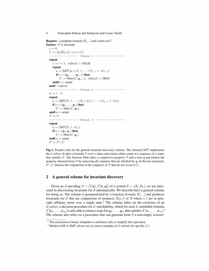
Require: a template formula R[ , ] and a term set UEnsure: P is invarianti := 0C :=

∧{R[s, t] | s, t ∈ U}

---------------- Phase 1 ----------------repeati := i+ 1; refined := FALSErepeata := SAT(I0 ∧ T1 ∧ · · · ∧ Ti−1 ∧ ¬Ci−1)if a = (q0, . . . , qi−1) thenC := filter(C, qi−1); refined := TRUE

until a = unsatuntil ¬refined---------------- Phase 2 ----------------k := i− 1repeata := SAT(T1 ∧ · · · ∧ Tk ∧ C0 ∧ · · · ∧ Ck−1 ∧ ¬Ck)if a = (q0, . . . , qk) thenC := filter(C, qk)

until a = unsatP := C---------------- Phase 3 ----------------repeata := SAT(T1 ∧ ¬C1)if a = (q0, q1) thenC := filter(C, q1)

until a = unsatP := P \ C

Fig. 1. Pseudo-code for the general invariant discovery scheme. The function SAT implementsthe L-solver. It takes a formula F over n states and returns either unsat or a sequence of n statesthat satisfies F . The function filter takes a conjunctive property P and a state q and returns theproperty obtained from P by removing all conjuncts that are falsified by q. In the last statement,P \ C denotes the conjunction of the conjuncts of P that do not occur in C.

2 A general scheme for invariant discovery

Given an L-encoding S = (I[x], T [x,y]) of a system S = (SI,ST), we are inter-ested in discovering invariants for S automatically. We describe here a general schemefor doing so. The scheme is parameterized by a template formula R[ , ] and producesinvariants for S that are conjunction of instances R[s, t] of R where s, t are in prin-ciple arbitrary terms over a single state.2 The scheme relies on the existence of anL-solver, a decision procedure for L-satisfiability, which for each L-satisfiable formulaF [x1, . . . ,xm] is also able to return a state list q1, . . . , qm that satisfiesF [x1, . . . ,xm].3

The scheme also relies on a procedure that can generate from S a non-empty instanti-

2 The restriction to binary templates is used here only to simplify the exposition.3 Modern SAT or SMT solvers are of course examples of L-solvers for specific L’s.


ation set U of terms over x to be used to generate the instance of R. In this setting, anaive approach would be to check every possible instanceR[s, t] individually for invari-ance. This would be highly impractical since the number of instances of R is quadraticin the size of the instantiation set U . In our approach, we check the satisfiability of allinstances at the same time and rely on the model generation ability of the L-solver toweed out several non-invariant instances at once.

The general scheme consists of a simple two-phase procedure, with an optionalthird phase. Given the formula R[ , ] and the term set U , the first phase starts with theoptimistic conjecture that the property

C[x] =∧

s,t∈U

R[s, t]

is invariant. Then, it uses the L-solver to weaken that conjecture by eliminating fromit as many conjuncts R[s, t] as possible—specifically, all conjuncts falsified by a k-reachable state, for some heuristically determined k. The resulting formula C is passedto the second phase, which attempts to prove C k-inductive by establishing the entail-ment (2) in Definition 1. Counterexamples to (2), i.e., models that falsify the entailment,are used to weaken C further by eliminating additional conjuncts until (2) holds. Thefinal formula—the empty conjunction in the worst case—is guaranteed to be invariant.That formula can be further processed in the optional third phase by removing fromit any conjunct that is a trivial invariant. The rationale for the last phase is that triv-ial invariants are never needed, for being directly implied by the formula encoding thetransition relation, and including them could put extra burden on the L-solver.

The pseudo-code for the procedure sketched above is provided in Figure 1. Thetermination condition for Phase 1 is a heuristic one: the search for the value k stopswhen C is falsified by no k-reachable states. Furthermore, every conjunct of C thatdoes not pass the test in Phase 2 is conservatively assumed not to be invariant (evenif it may be k′-inductive for some k′ > k) and removed. It is not difficult to showthat both phases are terminating. The final C is invariant because, by construction, it isk-inductive for the final k.

The practical feasibility of this invariant discovery scheme depends on the possibil-ity of representing the conjecture C compactly, i.e., by an equivalent formula using lessthan O(n2) space with n being the size of the instantiation set U , and refining it effi-ciently, i.e., in less than O(n2) time . This may not be the case in general for arbitrarytemplate formulasR[ , ]. Hence, we focus on a class of templates for which in practice,if not in theory, these space and time costs are sub-quadratic in n: L-formulas denotinga partial order. Common useful examples of partial orders include implication over theBooleans, the usual orderings over numeric domains, set inclusion over finite sets, aswell as equality over any domain.

3 Partial order templates

In this section, we describe two specializations of the general invariant discoveringscheme provided in Figure 1. Both specializations rely on the properties of partial or-ders in order to represent the conjunctive conjecture C compactly and process it effi-ciently. We start with one that works for any domain D and partial order � ⊆ D × D


provided that both the identity relation ≈ (i.e., equality) over D and the partial order �are expressible in a logic L with a decidable satisfiability problem. For example, this isthe case when L is rational (resp., linear integer) arithmetic and� is≤ or≥ over the ra-tional numbers (resp., the integers). Then, we discuss a further specialization for binarydomains. For simplicity, in both cases we assume that ≈ and � are built-in symbols ofL. As a consequence, the template R[ , ] will be just � .

Let U be again the given instantiation set, and let M be a sequence (q1, . . . , qm)of m ≥ 0 states from Q. To each t ∈ U we associate an m-vector vt where, fori = 1, . . . ,m, vt(i) is the value of t in state qi, i.e., the element of D that t evaluatesto in qi. The state sequence M induces an equivalence relation ≡M over the terms in Uwhere s ≡M t iff vs = vt.

Definition 2. Let M be a state sequence. Suppose ≡M has m equivalence classes andlet r1, . . . , rm be their respective representatives. Let the point-wise extension of � tom-vectors over D be denoted by � as well.4 The strongest conjecture CM consistentwith M is the smallest conjunction of ≈- and �-atoms that satisfies the following.

1. For each i = 1, . . . ,m and t ∈ U \ {ri}, CM contains t ≈ ri if t ≡M ri.2. For each distinct i, j = 1, . . . ,m, CM contains the atom ri � rj if vri � vrj .

We can specialize the procedure described in Figure 1 by using the formula CM

above instead of C where M is a sequence of states produced by the L-solver. Wedescribe this specialization in the following. We consider just Phase 1 since the otherphases are analogous.

Specializing the general scheme (Phase 1) For each iteration of the repeat loop inPhase 1 let M be the sequence of all the states generated until then (those passed tofilter in Figure 1). Initially, M is the empty sequence, which means that ≡M is U × Uand so CM has the form t2 ≈ t1 ∧ · · · ∧ tm ≈ t1 with {t1, . . . , tm} = U . Calls to filternow amount to computing the formula CM for the most recent M . This specializationmaintains the following (meta-)invariants on M : for all s, t ∈ U , (i) s ≡M t iff nonethe models generated by the L-solver so far falsifies the formula s ≈ t, i.e., contradictsthe conjecture that s ≈ t is invariant; (ii) vs � vt iff at least one of the models so farfalsifies the formula t � s but none falsify s � t; in other words, the evidence so fardisproves the conjecture that s ≈ t is invariant but not that s � t is.

Relying on the two properties above it possible to show that, at each step of Phase 1,the formula CM is L-equivalent to the formula C in Figure 1. The formula CM is morecompact than C because it replaces the quadratically many �-atoms between distinct≡M -equivalent terms by linearly-many equality atoms between these terms and theirequivalence class representative (e.g., {t2 ≈ t1, t3 ≈ t1} in place of {t1 � t2, t1 �t3, t2 � t3, t2 � t1, t3 � t1, t3 � t2}).

An even more compact version of CM is possible by exploiting the transitivity of�. In concrete, this can be done by computing a minimal, or close to minimal, basefor the poset (VM ,�) where VM = {vr1 , . . . ,vrm} (vr1 , . . . ,vrm are again the repre-sentatives of ≡M ’s classes). A base for the poset is a binary relation B on VM whose

4 So (u1, . . . , un) � (v1, . . . , vn) iff ui � vi for i = 1, . . . , n.


Require: (VM ,�) is a poset,Ensure: C is set of chains over VM , σ : VM → 2VM , and v � v′ for all v′ ∈ σ(v)C := ∅; σ := ∅for v ∈ VM doσ := σ ∪ {v 7→ ∅}for c ∈ C doi := greatestBelow(v, c)j := leastAbove(v, c)if j = 1 then

insert v at the beginning of celse

if i = j − 1 theninsert v at position j in c

elseif i = the length of c then

append v at the end of celse

if 0 < i thenadd v to σ(c(i))

if 0 < j thenadd c(j) to σ(v)

if v was not inserted into any chain thenC := C ∪ {[v]}

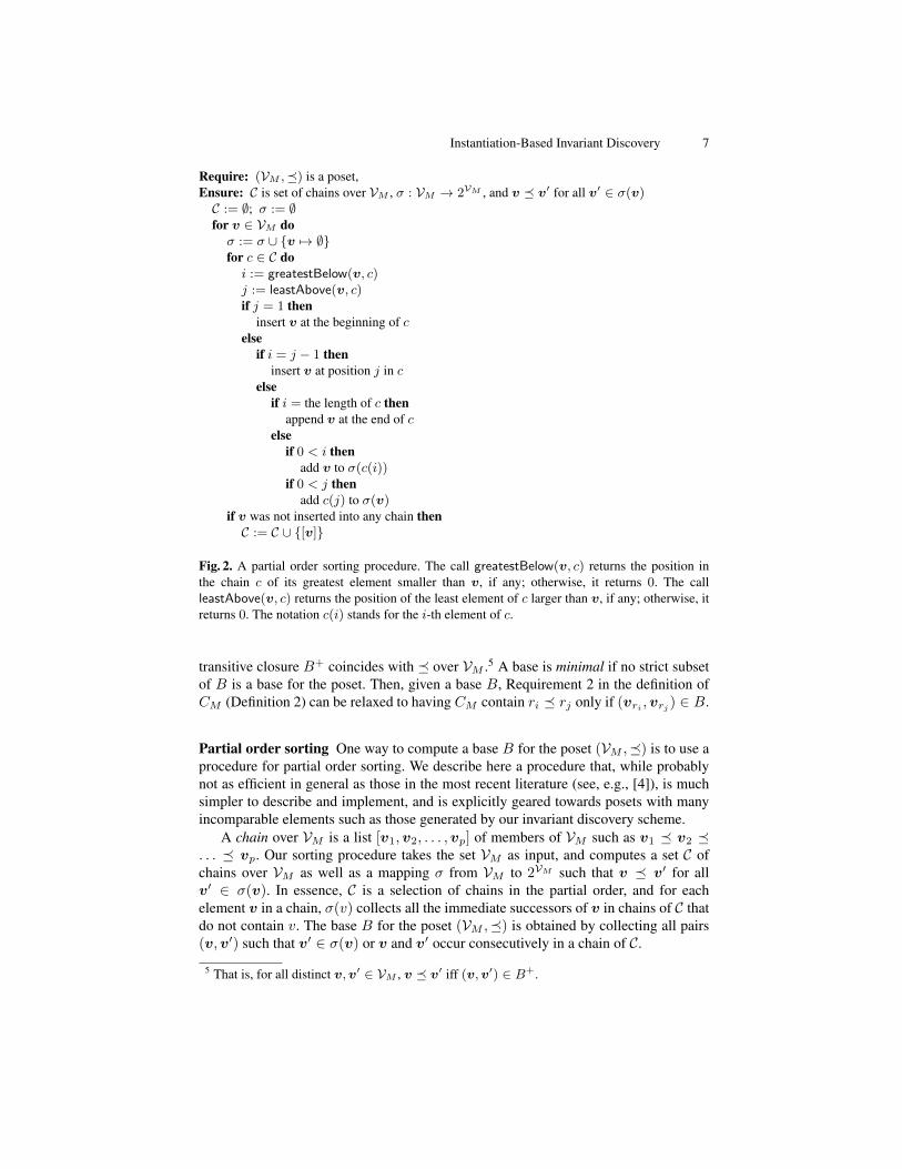
Fig. 2. A partial order sorting procedure. The call greatestBelow(v, c) returns the position inthe chain c of its greatest element smaller than v, if any; otherwise, it returns 0. The callleastAbove(v, c) returns the position of the least element of c larger than v, if any; otherwise, itreturns 0. The notation c(i) stands for the i-th element of c.

transitive closure B+ coincides with � over VM .5 A base is minimal if no strict subsetof B is a base for the poset. Then, given a base B, Requirement 2 in the definition ofCM (Definition 2) can be relaxed to having CM contain ri � rj only if (vri ,vrj ) ∈ B.

Partial order sorting One way to compute a base B for the poset (VM ,�) is to use aprocedure for partial order sorting. We describe here a procedure that, while probablynot as efficient in general as those in the most recent literature (see, e.g., [4]), is muchsimpler to describe and implement, and is explicitly geared towards posets with manyincomparable elements such as those generated by our invariant discovery scheme.

A chain over VM is a list [v1,v2, . . . ,vp] of members of VM such as v1 � v2 �. . . � vp. Our sorting procedure takes the set VM as input, and computes a set C ofchains over VM as well as a mapping σ from VM to 2VM such that v � v′ for allv′ ∈ σ(v). In essence, C is a selection of chains in the partial order, and for eachelement v in a chain, σ(v) collects all the immediate successors of v in chains of C thatdo not contain v. The base B for the poset (VM ,�) is obtained by collecting all pairs(v,v′) such that v′ ∈ σ(v) or v and v′ occur consecutively in a chain of C.

5 That is, for all distinct v,v′ ∈ VM , v � v′ iff (v,v′) ∈ B+.


The procedure, shown in Figure 2, works as follows. For each v ∈ VM and for eachexisting chain c ∈ C, it inserts v into c if possible. That is the case if, with respect to �,v is smaller than the first value of c, greater than the last, or in between two consecutiveelements of c. Otherwise, if c contains elements smaller than v, it adds v to the set σ(vi)where vi is the greatest of these elements; also, if c contains elements greater than v,it adds vj to the set σ(v) where vj is the least of these elements. If the procedure isunable to add v to any existing chain, it puts v in its own chain and adds that to C.

Example 1. We briefly illustrate the partial order sorting procedure where D is thedomain of the integers and � is the usual ≤ relation. Consider a sequence M withtwo states. Let s, t, q, r, p ∈ U be terms, and let the associated poset (VM ,�) be({vs,vt,vq,vr,vp},≤) where

vs = (6, 5), vt = (5, 2), vq = (5, 3), vr = (10, 2), vp = (2, 4) .

Initially, the chain C and the mapping σ are empty. The following table shows the valueof C and σ after each main iteration of the sorting procedure.

C σ1 [vs] vs 7→ ∅2 [vt,vs] vs 7→ ∅, vt 7→ ∅3 [vt,vq,vs] vs 7→ ∅, vt 7→ ∅, vq 7→ ∅, vr 7→ ∅4 [vt,vq,vs], [vr] vs 7→ ∅, vt 7→ {vr}, vq 7→ ∅, vr 7→ ∅5 [vt,vq,vs], [vr], [vp] vs 7→ ∅, vt 7→ {vr}, vq 7→ ∅, vr 7→ ∅, vp 7→ {vs}

ut

Analysis of the sorting procedure Our sorting procedure is trivially terminating be-cause the input VM is finite and the set C and map σ are initially empty. It is correctin the sense that the set B determined by C and σ is a base of (VM ,�). It is not opti-mal because it may produce non-disjoint chains, giving rise to non-minimal bases; but itseemed to work fairly well during the experimental evaluation we describe in Section 4.

A coarse-grained worst-case complexity analysis shows that the procedure has timecomplexity O(nwh), where w is the width of the poset (VM ,�), the cardinality of thelargest anti-chain in it, h is the height of the poset, the length of its longest chain, and nis the cardinality of VM .6 This analysis assumes that comparing two elements of VM for� takes constant time and that we store chains into arrays, which allows the functionsgreatestBelow and leastAbove in Figure 2 to be implemented by binary search. Theformer assumption does not generally hold because � is a point-wise ordering overvectors. One can make it only with a careful implementation based on the fact thatthe elements of VM are built incrementally at each round of the invariant discoveryprocedure: vectors of length k + 1 are obtained by adding a new component to vectorsof length k. Since (u1, . . . , uk+1) � (v1, . . . , vk+1) iff (u1, . . . , uk) � (v1, . . . , vk)and uk+1 � vk+1, by caching in a hash table the results of vector comparisons at roundk, vector comparisons at round k + 1 can be reduced to two constant time operations.7

6 Note that h ≤ n− w + 1, h = n when w = 1, and h = 1 when w = n.7 The hash table will have quadratic size only in the worst case when a linear number of vectors

are all pairwise comparable.


A recent and efficient partial sorting algorithm by Daskalakis et al. based on mergesort [4] has complexity O(w2n log n

w ), where again n is the cardinality of the posetand w its width. This complexity and that of our procedure do not easily compare ingeneral. But we note that the posets we work with tend to have a small height, becausemost value vectors are incomparable. Now, with an upper bound on a poset’s height,the poset’s width grows proportionally with its cardinality. This makes our procedurequadratic in n and the one by Daskalakis et al. more than cubic.

3.1 Binary domains

When the domain D has cardinality 2, for example in the Boolean case, there is a bet-ter way to compute a base B for the poset (VM ,�). Instead of a partial order sortingprocedure, we can use one that represents B more directly as a directed acyclic graph(dag) GM whose nodes are the equivalence classes of ≡M , and whose edges represent(selected) pairs in �. More precisely, the set of edges is such that for all distinct equiv-alence classes S and T of ≡M with respective representatives s and t, S and T areconnected in GM iff vs � vt. The graph for the initial, empty state sequence is simplythe graph with no edges and a single node, the whole instantiation set U .

Graph generation We developed a procedure to compute the graph GM for statesequences M , relying on the fact that each M is built incrementally, by appending anew state q to a previous sequence L. Given a sequence L and its graph GL, and anew state q, the procedure computes the graph GM for the sequence M obtained byappending q to L. We do not describe the procedure in detail here for space constraints.Instead, we give a general intuition on how it works.

Assume for concreteness that D = {0, 1} and 0 � 1, and let X be an arbitrarynode of the old graph GL. For i = 0, 1, let Xi be the set consisting of all the terms inX that evaluate to i in the new state q. The set Xi becomes a node of the new graphGM iff Xi 6= ∅. In other words, GM gets a node identical to X if all the terms of Xhave the same value in q, and gets two new nodes, partitioningX , otherwise. Wheneverboth X0 and X1 are added to GM , the edge X0 −→ X1 is also added. Edges betweenold nodes in GL are inherited by the corresponding new nodes consistently with theordering induced by M . In general, every edge Xi −→ Yj of GM (where X and Y arenodes of GL) comes from a path of length at most 2 from X to Y in GL; moreover,i ≤ j. The effect of the procedure is best illustrated with an example.

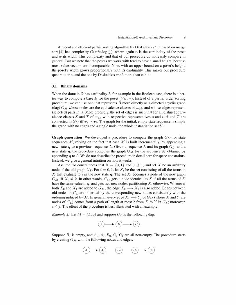
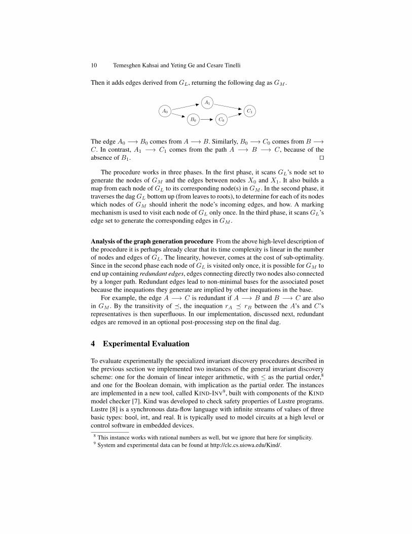
Example 2. Let M = (L, q) and suppose GL is the following dag.


vectors of length k + 1 are obtained by adding a new component to vectors oflength k. Since (u1, . . . , uk+1) � (v1, . . . , vk+1) iff (u1, . . . , uk) � (v1, . . . , vk) anduk+1 � vk+1, by caching in a hash table the results of vector comparisons atround k, vector comparisons at round k+1 can be reduced to two constant timeoperations.7 A recent and efficient partial sorting algorithm by Daskalakis et al.based on merge sort [?] has complexity O(w2n log n

w ), where again n is the sizeof the poset and w its width. This complexity and that of our procedure do noteasily compare in general. But we note that for posets with a small height, andso a width close to n, our procedure is basically quadratic in n while the one byDaskalakis et al. is cubic.

3.1 Binary domains

When the domain D has cardinality 2, for example in the Boolean case, there isa better way to compute a base B for the poset (VM ,�). Instead of the genericpartial order sorting procedure given earlier, we can use one that represents Bmore directly as a directed acyclic graph GM whose nodes are the equivalenceclasses of ≡M , and whose edges represent (selected) pairs in �. More precisely,the set of edges is such that for all distinct equivalence classes A and B of ≡M

with respective representatives rA and rB , A and B are connected in GM iffrA � rB . The graph for the initial state sequence, which is empty, is simply thegraph with no edges and a single node, the whole candidate set U .

We have developed a procedure to compute the graph GM for non-emptystate sequences M , relying on the fact that the M is built incrementally, byappending a new state q to a previous sequence L. The new procedure takes qand the dag GL as input, and produces GM as output. We do not describe theprocedure in full details here for space constraints. Instead, we give a generalintuition on how it works.

Assume for concreteness that D = {0, 1} and 0 � 1, and let A be an arbitrarynode of the old graph GL. For i = 0, 1, let Ai be the set consisting of all theterms in A that evaluate to i in the new state q. The set Ai becomes a node ofthe new graph GM iff Ai �= ∅. In other words, GM gets a node identical to A ifall the terms of A have the same value in q, and get two new nodes, partitioningA, otherwise. If both A0 and A1 are added to GM , the edge A0 −→ A1 isalso added. Edges between old nodes are inherited by the corresponding newnodes consistently with the ordering induced by M . The way this is done is bestillustrated with one example.

Example 3. Suppose GL is the following graph.

A B C

Suppose C1 is empty, and A0, A1, B0, C0 and C1 are all non-empty. Then theprocedure initially computes GM with the following nodes and edges.

7 Note that the hash table will have quadratic size only in the worst case when a linearnumber of vectors are all pairwise comparable.

Suppose B1 is empty, and A0, A1, B0, C0, C1 are all non-empty. The procedure startsby creating GM with the following nodes and edges.


A0 A1 B0 C0 C1

After that, it adds the edges derived from GL, producing the following finalversion of GM .

A0 A1

B0

C0 C1

The actual procedure

4 Experimental Evaluation

To evaluate experimentally the approaches described in the previous section wehave implemented two instances of the general invariant discovery scheme: onefor the domain of linear integer arithmetic, with the standard ≤ as the partialorder,8 and one for the Boolean domain, with implication as the partial order.The instances are implemented in a new tool, Kind-Inv, built on top of the Kindmodel checker [?]. Kind was developed to check safety properties of programswritten in the specification/programming Lustre [?]. Lustre is a synchronousdata-flow language operating on infinite streams of values of three basic types:bool, int, and real. It is typically used to model circuits at a high level orcontrol software in embedded devices.

Invariant generation for Lustre programs. More accurately, Kind is a k-induction-based model checker for programs in an idealized version of Lustrethat uses mathematical integers in place of machine integer values, and rationalnumbers in place of floating values. The underlying logic of Kind, and of Kind-Inv, is a quantifier-free logic that includes both propositional logic and lineararithmetic. We’ll refer to it as IL (for Idealized Lustre logic) here. The SMTsolvers CVC3 [?] and Yices [?] are used, in alternative, as satisfiability solvers forthis logic. Lustre programs can be readily encoded in IL as transition systemsof the sort described in the previous sections (see [?]) for more details).

A Lustre programs can be structured as a set of modules called nodes whichcan be understood as macros. Kind-Inv, however, takes a single-node Lustreprogram as input and automatically generates invariants for it. A multi-node

8 Actually, this instance works with rational numbers as well, but we will ignore thathere to simplify the exposition a bit.


Then it adds edges derived from GL, returning the following dag as GM .


A0 A1 B0 C0 C1

After that, it adds the edges derived from GL, producing the following finalversion of GM .

A0

B0 C0

C1

A1

The actual procedure


To evaluate experimentally the approaches described in the previous section wehave implemented two instances of the general invariant discovery scheme: onefor the domain of linear integer arithmetic, with the standard ≤ as the partialorder,8 and one for the Boolean domain, with implication as the partial order.The instances are implemented in a new tool, Kind-Inv, built on top of the Kindmodel checker [?]. Kind was developed to check safety properties of programswritten in the specification/programming Lustre [?]. Lustre is a synchronousdata-flow language operating on infinite streams of values of three basic types:bool, int, and real. It is typically used to model circuits at a high level orcontrol software in embedded devices.

Invariant generation for Lustre programs. More accurately, Kind is a k-induction-based model checker for programs in an idealized version of Lustrethat uses mathematical integers in place of machine integer values, and rationalnumbers in place of floating values. The underlying logic of Kind, and of Kind-Inv, is a quantifier-free logic that includes both propositional logic and lineararithmetic. We’ll refer to it as IL (for Idealized Lustre logic) here. The SMTsolvers CVC3 [?] and Yices [?] are used, in alternative, as satisfiability solvers forthis logic. Lustre programs can be readily encoded in IL as transition systemsof the sort described in the previous sections (see [?]) for more details).

A Lustre programs can be structured as a set of modules called nodes whichcan be understood as macros. Kind-Inv, however, takes a single-node Lustreprogram as input and automatically generates invariants for it. A multi-nodeprogram can be treated by a previous expansion to a behaviorally equivalentsingle-node one. The invariants discovered by Kind-Inv are added to the inputprogram as Lustre “assertions.” Contrary to other languages, assertions in Lustreare expressions of type bool that are assumed to be true at each execution step of

8 Actually, this instance works with rational numbers as well, but we will ignore thathere to simplify the exposition a bit.

The edge A0 −→ B0 comes from A −→ B. Similarly, B0 −→ C0 comes from B −→C. In contrast, A1 −→ C1 comes from the path A −→ B −→ C, because of theabsence of B1. ut

The procedure works in three phases. In the first phase, it scans GL’s node set togenerate the nodes of GM and the edges between nodes X0 and X1. It also builds amap from each node of GL to its corresponding node(s) in GM . In the second phase, ittraverses the dagGL bottom up (from leaves to roots), to determine for each of its nodeswhich nodes of GM should inherit the node’s incoming edges, and how. A markingmechanism is used to visit each node of GL only once. In the third phase, it scans GL’sedge set to generate the corresponding edges in GM .

Analysis of the graph generation procedure From the above high-level description ofthe procedure it is perhaps already clear that its time complexity is linear in the numberof nodes and edges of GL. The linearity, however, comes at the cost of sub-optimality.Since in the second phase each node of GL is visited only once, it is possible for GM toend up containing redundant edges, edges connecting directly two nodes also connectedby a longer path. Redundant edges lead to non-minimal bases for the associated posetbecause the inequations they generate are implied by other inequations in the base.

For example, the edge A −→ C is redundant if A −→ B and B −→ C are alsoin GM . By the transitivity of �, the inequation rA � rB between the A’s and C’srepresentatives is then superfluous. In our implementation, discussed next, redundantedges are removed in an optional post-processing step on the final dag.


To evaluate experimentally the specialized invariant discovery procedures described inthe previous section we implemented two instances of the general invariant discoveryscheme: one for the domain of linear integer arithmetic, with ≤ as the partial order,8

and one for the Boolean domain, with implication as the partial order. The instancesare implemented in a new tool, called KIND-INV9, built with components of the KINDmodel checker [7]. Kind was developed to check safety properties of Lustre programs.Lustre [8] is a synchronous data-flow language with infinite streams of values of threebasic types: bool, int, and real. It is typically used to model circuits at a high level orcontrol software in embedded devices.

8 This instance works with rational numbers as well, but we ignore that here for simplicity.9 System and experimental data can be found at http://clc.cs.uiowa.edu/Kind/.


KIND is a k-induction-based model checker for programs in an idealized version ofLustre that uses (mathematical) integers in place of machine integer values, and rationalnumbers in place of floating values. The underlying logic of KIND, and of KIND-INV,is a quantifier-free logic that includes both propositional logic and linear arithmetic.We’ll refer to it as IL (for Idealized Lustre logic) here. Lustre programs can be readilyencoded in IL as transition systems of the sort we use here (see [7] for more details).The SMT solvers CVC3 [1] and Yices [5] are used, in alternative, as satisfiability solversfor this logic. A Lustre program can be structured as a set of modules called nodeswhich can be understood as macros. KIND-INV currently takes a single-node Lustreprogram as input. A multi-node program can be treated by expanding it in advance toa behaviorally equivalent single-node one. The invariants discovered by KIND-INV arethen added to the Lustre input program as “assertions.” Contrary to other languages,such as C, assertions in Lustre are expressions of type bool that are assumed to be trueat each execution step of the program.

KIND-INV accepts two options for generating invariants: bool and int. The firstoption produces invariants of the form s→ t or s = t where s and t are Lustre Booleanterms. The second produces invariants of the form s ≤ t or s = t where s and t areinteger terms. The instantiation set U currently consists of heuristically selected termsfrom the input Lustre program plus some distinguished constant terms such as true andfalse. Note that bool terms may contain int terms, as in (x + y > 0) or done, and viceversa, as in x + (if y > 0 then y else 1).

KIND-INV provides three binary options affecting invariant generation. The firsttwo work only with the bool invariant option, the last one with both options:

No Ands : When this flag is turned on, KIND-INV will not consider candidate terms ofthe form s∧ t. The rationale behind this flag is that, conjunctive terms lead to manytrivial invariants, for instance, those of the form (s ∧ t) → s. Having too many ofthese unnecessary invariants can be burdensome for the SMT-solver, limiting theeffectiveness of the non-trivial invariants in the generated assertion.

No Redundant Edges : When this flag is on, KIND-INV will remove redundant edgesfrom the final dag storing the computed poset (see Section 3.1).

No Trivial Invariants : This flags governs whether the third phase of the invari-ant discovery procedure is performed or not. Its rationale is that the third phase isexpensive and may not be worthwhile.

Evaluation setup To evaluate KIND-INV, we used a benchmark set derived fromthe one used in [7], which consists of a variety of benchmarks from several sources.Each benchmark in the original set is a Lustre program together with a single prop-erty to check, expressed as a Lustre bool term. Our derived set discards some duplicatebenchmarks—included in the original set by mistake—and converts each program to asingle-node one using the pollux tool from the Lustre 4 distribution.

Let us call a benchmark valid if its safety property holds for the associated program,and invalid otherwise. KIND is able to prove 438 of the 941 benchmarks in our setinvalid by returning a (independently verified) counter-example trace for the program.KIND reports 309 of the remaining benchmarks as valid, and diverges on the remaining194 benchmarks, even with very large timeout values. We conjecture that those 194


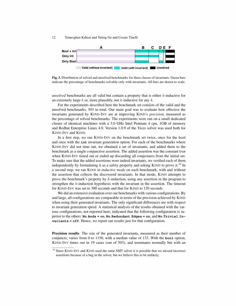
Fig. 3. Distribution of solved and unsolved benchmarks for three classes of invariants. Green barsindicate the percentage of benchmarks solvable only with invariants. All bars are drawn to scale.

unsolved benchmarks are all valid but contain a property that is either k-inductive foran extremely large k or, more plausibly, not k-inductive for any k.

For the experiments described here the benchmark set consists of the valid and theunsolved benchmarks, 503 in total. Our main goal was to evaluate how effective theinvariants generated by KIND-INV are at improving KIND’s precision, measured asthe percentage of solved benchmarks. The experiments were run on a small dedicatedcluster of identical machines with a 3.0 GHz Intel Pentium 4 cpu, 1GB of memoryand Redhat Enterprise Linux 4.0. Version 1.0.9 of the Yices solver was used both forKIND-INV and KIND.

In a first step, we ran KIND-INV on the benchmark set twice, once for the booland once with the int invariant generation option. For each of the benchmarks whereKIND-INV did not time out, we obtained a set of invariants, and added them to thebenchmark as a single conjunctive assertion. The added assertion was the constant truewhen KIND-INV timed out or ended up discarding all conjectures from the initial set.To make sure that the added assertions were indeed invariants, we verified each of themindependently by formulating it as a safety property and asking KIND to prove it.10 Ina second step, we ran KIND in inductive mode on each benchmark, with and withoutthe assertion that collects the discovered invariants. In that mode, KIND attempts toprove the benchmark’s property by k-induction, using any assertion in the program tostrengthen the k-induction hypothesis with the invariant in the assertion. The timeoutfor KIND-INV was set to 300 seconds and that for KIND to 120 seconds.

We did an extensive evaluation over our benchmarks with various configurations. Byand large, all configurations are comparable in terms of the precision achieved by KINDwhen using their generated invariants. The only significant differences are with respectto invariant generation speed. A statistical analysis of the results obtained with the var-ious configurations, not reported here, indicated that the following configuration is su-perior to the others: No Ands = on, No Redundant Edges = on, and No Trivial In-variants = off. Hence, we report our results just for that configuration.

Precision results The size of the generated invariants, measured as their number ofconjuncts, varies from 0 to 1150, with a median value of 133. With the bool option,KIND-INV times out in 19 cases (out of 503), and terminates normally but with an

10 Since KIND-INV and KIND used the same SMT solver it is possible that we missed incorrectassertions because of a bug in the solver, but we believe this to be unlikely.


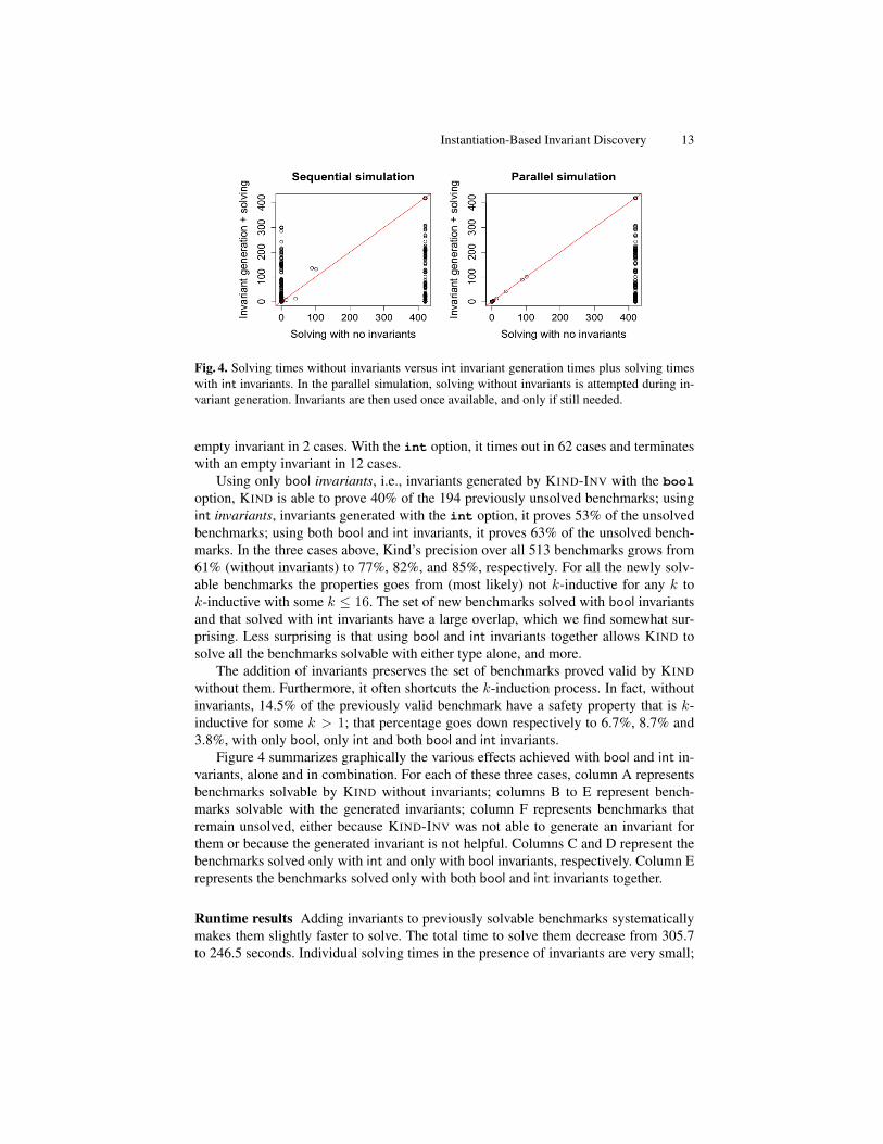
Fig. 4. Solving times without invariants versus int invariant generation times plus solving timeswith int invariants. In the parallel simulation, solving without invariants is attempted during in-variant generation. Invariants are then used once available, and only if still needed.

empty invariant in 2 cases. With the int option, it times out in 62 cases and terminateswith an empty invariant in 12 cases.

Using only bool invariants, i.e., invariants generated by KIND-INV with the booloption, KIND is able to prove 40% of the 194 previously unsolved benchmarks; usingint invariants, invariants generated with the int option, it proves 53% of the unsolvedbenchmarks; using both bool and int invariants, it proves 63% of the unsolved bench-marks. In the three cases above, Kind’s precision over all 513 benchmarks grows from61% (without invariants) to 77%, 82%, and 85%, respectively. For all the newly solv-able benchmarks the properties goes from (most likely) not k-inductive for any k tok-inductive with some k ≤ 16. The set of new benchmarks solved with bool invariantsand that solved with int invariants have a large overlap, which we find somewhat sur-prising. Less surprising is that using bool and int invariants together allows KIND tosolve all the benchmarks solvable with either type alone, and more.

The addition of invariants preserves the set of benchmarks proved valid by KINDwithout them. Furthermore, it often shortcuts the k-induction process. In fact, withoutinvariants, 14.5% of the previously valid benchmark have a safety property that is k-inductive for some k > 1; that percentage goes down respectively to 6.7%, 8.7% and3.8%, with only bool, only int and both bool and int invariants.

Figure 4 summarizes graphically the various effects achieved with bool and int in-variants, alone and in combination. For each of these three cases, column A representsbenchmarks solvable by KIND without invariants; columns B to E represent bench-marks solvable with the generated invariants; column F represents benchmarks thatremain unsolved, either because KIND-INV was not able to generate an invariant forthem or because the generated invariant is not helpful. Columns C and D represent thebenchmarks solved only with int and only with bool invariants, respectively. Column Erepresents the benchmarks solved only with both bool and int invariants together.

Runtime results Adding invariants to previously solvable benchmarks systematicallymakes them slightly faster to solve. The total time to solve them decrease from 305.7to 246.5 seconds. Individual solving times in the presence of invariants are very small;


on average just 0.95s for all solvable benchmarks. In addition to the substantial in-crease in precision, this provides further evidence that our invariant discovery proce-dure produces high quality invariants. Invariant generation has of course its own, non-insignificant cost. Over the whole benchmark set, KIND-INV runtimes vary from lessthan a second to hundreds of seconds, to timing out at 300s. However, their medianvalue is fairly small: 22.4s for int invariants and just 6.3s for bool ones. For the greatmajority of benchmarks (84%) bool invariant generation takes less than a minute perbenchmark.

Evaluating invariant generation costs against the increase in precision is a diffi-cult task because it also depends on the relative importance of precision versus promptresponse. A supporting argument is that invariant generation and k-induction modelchecking can be done in parallel—with invariants fed to the k-induction loop as soonas they are generated—mitigating this way the cost of invariant generation. Develop-ing a parallel model checker integrating KIND and KIND-INV was beyond the scope ofthis work. An approximate analysis, however, can be provided with a rough conceptualsimulation of such a concurrent system.

Since the synchronization overhead in the parallel model checker would be arguablyvery small, we can ignore it here for simplicity. Then we can imagine the parallelchecker’s runtimes to be, for each benchmark, the minimum between the followingtwo values: (i) the time KIND takes to prove the property without invariants and (ii)the sum of the times KIND-INV takes to output an invariant and KIND takes to provethe property using that invariant. The scatter plots in Figure 4 illustrate this comparisonwith int invariants—the results are similar for bool invariants. The first plot comparesfor each benchmark the runtime of KIND with no invariants and a 420s timeout11 againstthe runtime of a hypothetical sequential checker that uses KIND-INV with a timeout of120s, to add an invariant to the program, and then calls KIND with a timeout of 300s.The considerable invariant generation time penalty paid by the sequential checker (il-lustrated by all the points above the diagonal lines in the first plot) essentially disappearswith the parallel checker, as shown in the second plot.

5 Conclusion and Future Work

We presented a novel scheme for discovering invariants in transition systems. Thescheme is parametrized by a formula template representing a decidable relation over thesystem’s datatypes, and by a set of terms used to instantiate the template. Its main fea-tures are that it checks all template instances for invariance at the same time and makesheavy use of a satisfiability solver for the logic in which the system and the instancesare encoded. We described two specializations of the scheme to templates representingpartial orders where we can exploit the properties of posets to achieve space and timeefficiencies. Initial experimental results are very encouraging in terms of the speed ofinvariant generation and the effectiveness of the generated invariants in automating theverification of safety properties.

In the implementation discussed in the previous section, invariant generation is doneoff-line. We are developing a parallel model checking architecture and implementation11 Increasing the timeout from 300s to 420s does not change the set of solved benchmarks.


in which k-induction and invariant generation are done concurrently, with invariants fedto the k-induction loop as soon as they are produced.

Our invariant discovery scheme lumps together, in a single invariant produced atthe end, instances of the template that may be k-inductive for different values of k.We believe that the effectiveness of the parallel model checking architecture would in-crease if invariant instances were identified and output progressively—with k-inductiveinstances produced before (k + 1)-inductive ones. We are working on a new version ofthe scheme based on this idea.

We are also investigating techniques for compositional reasoning with synchronoussystems based on the invariant discovery method presented in this paper. The main ideais to generate invariants separately for each module of a multi-module system, and thenuse them to aid the verification of properties of the entire system.

References

1. C. Barrett and C. Tinelli. CVC3. In W. Damm and H. Hermanns, editors, CAV’07, volume4590 of LNCS, 2007.

2. S. Bensalem and Y. Lakhnech. Automatic generation of invariants. Form. Methods Syst.Des., 15(1):75–92, 1999.

3. S. Das and D. L. Dill. Counter-example based predicate discovery in predicate abstraction.In FMCAD ’02, pages 19–32. Springer-Verlag, 2002.

4. C. Daskalakis, R. M. Karp, E. Mossel, S. Riesenfeld, and E. Verbin. Sorting and selection inposets. In ACM-SIAM Symposium on Discrete Algorithms, pages 392–401, 2009.

5. B. Dutertre and L. de Moura. The YICES SMT solver. Technical report, SRI International,2006.

6. S. Gulwani, S. Srivastava, and R. Venkatesan. Constraint-based invariant inference overpredicate abstraction. In VMCAI ’09, pages 120–135, Berlin, Heidelberg, 2009.

7. G. Hagen and C. Tinelli. Scaling up the formal verification of lustre programs with SMT-based techniques. In FMCAD ’08, pages 1–9, Piscataway, NJ, USA, 2008. IEEE Press.

8. N. Halbwachs, P. Caspi, P. Raymond, and D. Pilaud. The synchronous data-flow program-ming language LUSTRE. Proceedings of the IEEE, 79(9):1305–1320, September 1991.

9. W. Hunt, S. Johnson, P. Bjesse, and K. Claessen. SAT-Based Verification without State SpaceTraversal, volume 1954, pages 409–426. Springer Berlin / Heidelberg, 2000.

10. Z. Manna and A. Pnueli. Temporal Verification of Reactive Systems: Safety. Springer-Verlag,1995.

11. S. Pandav, K. Slind, and G. Gopalakrishnan. Counterexample guided invariant discovery forparameterized cache coherence protocol verification. In CHARME 2005, pages 317–331,2005. LNCS 2144.

12. S. Srivastava and S. Gulwani. Program verification using templates over predicate abstrac-tion. SIGPLAN Not., 44:223–234, 2009.

13. J. X. Su, D. L. Dill, and C. W. Barrett. Automatic generation of invariants in processorverification. In In FMCAD ’96, volume 1166 of LNCS, pages 377–388, 1996.

14. M. Thalmaier, M. D. Nguyen, M. Wedler, D. Stoffel, J. Bormann, and W. Kunz. Analyzingk-step induction to compute invariants for SAT-based property checking. In DAC ’10, pages176–181. ACM, 2010.

15. A. Tiwari, H. Rueß, H. Saı̈di, and N. Shankar. A technique for invariant generation. InTACAS ’01, pages 113–127. Springer-Verlag, 2001.

Documents

Instantiation-Based Invariant Discoveryhomepage.cs.uiowa.edu/~tinelli/papers/KahGT-NFM-11.pdf · Instantiation-Based Invariant Discovery? ... previous approaches is its ability to