Instantaneous Real-time Cycle-slip Correction of Dual-frequency GPS Data

Donghyun Kim and Richard B. Langley

Geodetic Research Laboratory, Department of Geodesy and Geomatics Engineering, University of New Brunswick, Fredericton, N.B., Canada E3B 5A3

kim@unb.ca and lang@unb.ca

BIOGRAPHIES Donghyun Kim is a post-doctoral fellow in the Department of Geodesy and Geomatics Engineering at the University of New Brunswick (UNB), where he has been developing a new on-the-fly (OTF) ambiguity resolution technique for long-baseline kinematic GPS applications and software for a gantry crane auto-steering system using the carrier-phase observations of high data rate GPS receivers. He has a B.Sc., M.S. and Ph.D. in geomatics from Seoul National University. He has been involved in GPS research since 1991 and is a member of the IAG Special Study Group “Wide Area Modeling for Precise Satellite Positioning”.

Richard Langley is a professor in the Department of Geodesy and Geomatics Engineering at UNB, where he has been teaching and conducting research since 1981. He has a B.Sc. in applied physics from the University of Waterloo and a Ph.D. in experimental space science from York University, Toronto. Prof. Langley has been active in the development of GPS error models since the early 1980s and is a contributing editor and columnist for GPS World magazine. ABSTRACT Errors such as cycle slips, receiver clock jumps, multipath, diffraction, ionospheric scintillation, etc., which are apt to be unspecified in functional and stochastic models, must be correctly detected and removed or otherwise handled at the data quality control stage either for real-time or post-processing needs in order to attain high precision positioning and navigation results with the GPS carrier-phase measurements. The result of incorrect or incomplete quality control, particularly for cycle slips, can be problematic in applications using the carrier-phase measurements because it introduces artificial biases into the observations and subsequently, the estimated parameter values. In this paper, we propose a new cycle-slip correction method which enables instantaneous (i.e., using only the current epoch’s measurements) cycle-slip correction at the

data quality control stage and can operate in real time. Our approach utilizes dual-frequency carrier phases. The method includes: 1) two parameters for generating and filtering cycle-slip candidates; and 2) validation procedures which authenticate correct cycle slips. Compared with conventional approaches utilizing carrier phases and pseudoranges, our approach does not require a smoothing or filtering process to reduce observation noise and provides instantaneous cycle-slip correction, so that it is possible to implement the algorithm for real-time applications. Test results carried out in a variety of situations including short-baseline, long-baseline, static, kinematic, low-dynamics, high-dynamics, low-data rate, high-data rate, real-time, and post-processing modes have confirmed the completeness of our approach. INTRODUCTION In order to attain consistent high-precision positioning results with the GPS carrier-phase measurements, errors unspecified in a functional or stochastic model (errors of omission) must be correctly detected and removed or otherwise handled at the data processing stage. Such errors in the carrier-phase measurements may include cycle slips, receiver clock jumps, multipath, diffraction, ionospheric scintillation, etc. Reliability, which refers to the ability to detect such errors and to estimate the effects that they may have on a solution, is one of the main issues in quality control. Texts containing detailed discussions of this topic include Leick [1995] and Teunissen [1998]. A comprehensive investigation of quality issues in real-time GPS positioning has been carried out by the Special Study Group 1.154 of the International Association of Geodesy during 1996-1999 [Rizos, 1999]. The effects of cycle slips and receiver clock jumps can be easily captured either in the measurement or parameter domain due to their systematic characteristics. Their systematic effects on the carrier-phase measurements can be almost completely removed once they are correctly detected and identified. On the other hand, multipath, diffraction, ionospheric scintillation, etc. have temporal

and spatial characteristics which are more or less quasi-random (we will see some examples in the section of “Test Results”). These quasi-random errors cannot be completely eliminated and must be handled using a rigorous mathematical approach such as the data snooping theory [Baarda, 1968]. However, statistical testing and reliability analysis can only be efficient if the stochastic models are correctly known or well approximated. As has been experienced, quasi-random errors (e.g., multipath, diffraction, ionospheric scintillation, etc.) are often mixed with systematic ones (e.g., cycle slips and receiver clock jumps) in real world situations. One reasonable approach for handling errors in such situations is to separate the systematic ones from the quasi-random ones. Estimating the quasi-random errors after removing the systematic ones can provide more reliable results in terms of least-squares estimation. This is the main idea implemented in our quality control algorithm including cycle-slip correction. This paper addresses the development of a cycle-slip correction technique designed to detect and correct cycle slips in dual-frequency carrier phase data in a real-time environment as a part of a quality control algorithm. Our approach was originally developed for real-time GPS kinematic applications requiring sub-centimetre accuracy with high-rate data (e.g., 10 Hz). For the completeness of our discussions, we will look at the characteristics of errors of interest in the first place. Then, a brief explanation of our approach for cycle-slip correction will be given. Several difficult situations, which can be considered as the worst cases in real world situations, will be discussed to answer in the end the question: “How perfectly can the method work?” Finally, conclusions will follow the test results and discussions. ABNORMAL BEHAVIOUR OF OBSERVATION DATA The quality of GPS positioning is dependent on a number of factors. For attaining high-precision positioning results, we need to identify the main error sources impacting on the quality of the observations. In terms of data processing, cycle slips, receiver clock jumps and quasi-random errors are the main sources which can deteriorate the quality of the observations and subsequently, the quality of positioning results. Cycle Slips Cycle slips are discontinuities of an integer number of cycles in the measured (integrated) carrier phase resulting from a temporary loss-of-lock in the carrier tracking loop of a GPS receiver. In this event, the integer counter is reinitialized which causes a jump in the instantaneous accumulated phase by an integer number of cycles.

Three causes of cycle slips can be distinguished [Hofmann-Wellenhof et al., 1997]: First, cycle slips are caused by obstructions of the satellite signal due to trees, buildings, bridges, mountains, etc. The second cause of cycle slips is a low signal-to-noise ratio (SNR) or alternatively carrier-to-noise-power-density ratio (C/N0) due to bad ionospheric conditions, multipath, high receiver dynamics, or low satellite elevation angle. A third cause is a failure in the receiver software which leads to incorrect signal processing. Cycle slips in the phase data must be corrected to utilize the full measurement strength of the phase observable. The process of cycle-slip correction involves detecting the slip, estimating the exact number of L1 and L2 frequency cycles that comprise the slip, and actually correcting the phase measurements by these integer estimates. Cycle slip detection and correction requires the location of the jump and the determination of its size. It can be completely removed once it is correctly detected and identified. Receiver Clock Jumps Most receivers attempt to keep their internal clocks synchronized to GPS Time. This is done by periodically adjusting the clock by inserting time jumps. The actual mechanism of receiver clock jumps is typically proprietary. However, like cycle slips, their effects on the code and phase observables are more or less known to users and hence it is possible to remove almost completely their effects. We have experienced two typical cases with different receivers: millisecond jumps and time slues. Some receivers (e.g., the Ashtech Z-12) always keep their clocks synchronized to GPS Time within ± 1 millisecond. When the clock offset becomes larger than ± 1 millisecond, the receiver corrects the clock by ± 1 millisecond. At the moment of the clock correction, two main effects are transferred into the code and phase observables: i.e., ± 1 millisecond clock offset and geometric range change corresponding to the offset. The clock jumps can be easily detected in both the measurement and parameter domains. The effects of the clock jumps in the phase observables can be corrected by the Doppler frequency. According to our recent investigation of the Navcom NCT-2000D receiver, it has quite a sophisticated algorithm for keeping its clock synchronized to GPS Time within a few microseconds. When the clock bias reaches a certain threshold (e.g., 4 microseconds), it slues the clock bias. Arbitrary integer cycles of L1 and L2 phase (e.g., several times 1540 cycles of L1 phase or 1200 cycles of L2 phase) are added to the code and phase observables. The clock slues can be easily detected and corrected in either the measurement or parameter domains.

Quasi-random Errors Since least-squares estimation when errors are present tends to hide (reduce) their impact and distribute their effects throughout the entire set of measurements, it is better to handle cycle slips and clock jumps separately from quasi-random errors. Multipath, diffraction, ionospheric scintillation, etc. may be the main sources of the quasi-random errors, which are apt to be omitted in the functional and stochastic models. To detect and remove them, we have to test a null hypothesis (that is, no errors in the measurements) against an alternative hypothesis which describes the type of misspecifications in the models (see Leick [1995] and Teunissen [1998]). AN INSTANTANEOUS CYCLE-SLIP CORRECTION TECHNIQUE One of the various methods for detecting and identifying cycle slips is to obtain the triple-difference (TD) observations of carrier phases first. By triple differencing the observations (that is, at two adjacent data collection epochs differencing double-difference (DD) observations which is differencing between receivers followed by differencing between satellites) biases such as the clock offsets of the receivers and GPS satellites, and ambiguities can be removed. The TD observables (in distance per second units) are

1 1 1

1 1

2 2 2

2 2 ,

C s

I b

C s

I b

δ δ ρ λ δ τ δδ δ δ ε

δ δ ρ λ δ τ δγ δ δ δ ε

∇∆Φ = ∇∆ + ⋅∇∆ + ∇∆ + ∇∆− ∇∆ + ∇∆ + ∇∆

∇∆Φ = ∇∆ + ⋅∇∆ + ∇∆ + ∇∆− ⋅ ∇∆ + ∇∆ + ∇∆

(1)

where Φ is the measured carrier phase; ρ is the

geometric range from receiver to GPS satellite; λ is the carrier wavelength ; C is a potential cycle slip (in cycle units); τ is the delay due to the troposphere; s is the satellite orbit bias; I is the delay of L1 carrier phase due to the ionosphere; 2

2 1( / ) 1.65γ λ λ= ≈ ; b is multipath; ε is receiver system noise; subscripts “1” and “2” represent L1 and L2 carrier phases, respectively; and ∇∆ and δ∇∆ are the DD and TD operators, respectively. In most GPS applications, regardless of surveying modes (static and kinematic) and baseline lengths (short, medium and long), the effects of the triple-differenced biases and noise (i.e., atmospheric delay, satellite orbit bias, multipath, and receiver system noise) are more or less below a few centimetres as long as observation sampling interval is relatively short (e.g., sampling interval less than 1 minute). There could be exceptional situations such as an ionospheric disturbance, extremely long baselines,

and huge (rapid) variation of the heights of surveying points in which the combined effects of the biases and noise can exceed the wavelengths of L1 and L2 carrier phases. However, to simplify our discussion, we will assume, for the time being, that such situations can be easily controlled through adjusting the sampling rate so that the combined effects of the biases and noise can be reduced below a few centimetres. In the section of “Cycle-slip Candidates”, we will see that we can remove this assumption. Cycle-slip Observables As revealed in Eq. (1), the geometric range should be removed to estimate the size of cycle slips. If we can replace the TD geometric ranges with their estimates, then the TD carrier-phase prediction residuals become

1 1 1 1 1

2 2 2 2 2

ˆ

ˆ ,TD

TD

C

C

δ δ δ ρ λ εδ δ δ ρ λ ε

′Φ = ∇∆Φ − ∇∆ = ⋅∇∆ +′Φ = ∇∆Φ − ∇∆ = ⋅∇∆ +

(2)

where

1 1 1

2 2 2 ,TD

TD

s I b

s I b

ε δρ δ τ δ δ δ δ εε δρ δ τ δ γ δ δ δ ε

′ = + ∇∆ + ∇∆ − ∇∆ + ∇∆ + ∇∆′ = + ∇∆ + ∇∆ − ⋅ ∇∆ + ∇∆ + ∇∆

(3)

and ˆ( )TDδρ δ ρ δ ρ= ∇∆ − ∇∆ represents the prediction residuals of TD geometric ranges. As seen in Eqs. (2) and (3), therefore, the TD carrier-phase prediction residuals will be a good measure for detecting and correcting cycle slips if the effects of the residuals in Eq. (3) are small. TD Geometric Range Estimation To obtain the estimates of the TD geometric ranges, we need an other observable which is immune from cycle slips. The Doppler frequency and the TD pseudoranges can be used for this purpose. The former is preferable to reduce the effects of the residuals in Eq. (3). Using the Doppler frequency at two adjacent data collection epochs, we have

( )1ˆ / 2k k kD Dδ ρ −∇∆ = − ∇∆ + ∇∆ , (4)

where D is the Doppler frequency (in distance per second units); subscripts “k” and “k-1” represent the time tags of two adjacent data collection epochs and the sign is reversed due to the definition of Doppler shift. For some receivers for which the Doppler frequency is not available to users, the TD pseudoranges (somewhat nosier than the Doppler frequency) can be used instead. Then the estimates of the TD geometric ranges are given as:

( )1ˆ /k k kP P tδ ρ δ δ δ−∇∆ = ∇∆ − ∇∆ , (5)

where P is the measured pseudorange and 1( )k kt t tδ −= − is the time interval between two adjacent data collection epochs. Cycle-slip Candidates Consider the first two moments of the TD carrier-phase prediction residuals

[ ][ ]

, 1, 2

,

TDi i i

TDi TDi

E C i

Cov Q

δ λ

δ

Φ = ⋅∇∆ =

Φ = (6)

where [ ]E ⋅ and [ ]Cov ⋅ are the mathematical expectation

and variance-covariance operators. Since there is no redundancy to carry out statistical testing for Eq. (6), we will use it to obtain the cycle-slip candidates. In this case, we need a priori information for the second moment. This can be obtained either through system tuning or adaptive estimation. This means that we do not have to assume specific models for the biases and noise in Eq. (3). Filtering of Cycle-slip Candidates When dual-frequency carrier phases are available, we can reduce, to a large extent, the number of cycle-slip candidates using the TD geometry-free phase (a scaled version of which is called the ionospheric delay rate). The TD geometry-free phase (in distance per second units) is

( )1 2

1 1 2 2 ,GF

C C

δ δ δ

λ λ ε

Φ = ∇∆Φ − ∇∆Φ

′′= ⋅∇∆ − ⋅∇∆ + (7)

where

( ) ( ) ( )1 2 1 21 I b bε γ δ δ δ δ ε δ ε′′ = − ∇∆ + ∇∆ − ∇∆ + ∇∆ − ∇∆ .

(8) Compared with Eq. (3), the effects of the residuals in Eq. (8) are much smaller. We can also consider the first two moments of the TD geometry-free phase

[ ][ ]

1 1 2 2

.

GF

GF GF

E C C

Cov Qδ

δ λ λ

δ

Φ = ⋅∇∆ − ⋅∇∆

Φ = (9)

In conjunction with Eq. (6), Eq. (9) can be used to filter out most cycle-slip candidates which are not real cycle slips. An exceptional case is the combination-insensitive cycle-slip pairings of which the expectation in Eq. (9) is close to zero. Cycle-slip Validation Fixing cycle slips in the TD observations is conceptually the same problem as resolving ambiguities in the DD

observations. Consider the linearized model of the TD observables in Eq. (1):

[ ], ,

,

n u

Cov

= + + ∈ ∈

=

y Ac Bx e c x

y Q

¢ ¡ (10)

where y is the 1n× vector of the difference between the TD observations and their computed values; n is the number of measurements; c is the 1n× vector of the cycle-slip candidates; x is the 1u × vector of all other unknown parameters including position and other parameters of interest; u is the number of all other unknowns except cycle slips; A and B are the design matrices of the cycle-slip candidates and the other unknown parameters; e is the 1n× vector of the random errors. The first step for cycle-slip validation is to search for the best and second best cycle-slip candidates which minimize the quadratic form of the residuals. The residuals of least-squares estimation for cycle-slip candidates are given as:

ˆ ˆ′= −v y Bx , (11) where

( )ˆ .

′ = −

′=-1T -1 T -1

y y Ac

x B Q B B Q y (12)

Then, discrimination power between two candidates is measured by comparing their likelihood. We follow a conventional discrimination test procedure similar to that described by Wang et al. [1998]. A test statistic for cycle-slip validation is given by

d = Ω − Ωc1 c2 , (13)

where Ωc1 and Ωc2 are the quadratic form of the residuals of the best and second best candidates. A statistical test is performed using the following null and alternative hypotheses:

[ ] [ ]0 1: 0, : 0H E d H E d= ≠ . (14)

A test statistic for testing the above hypotheses is given by

( )d

WCov d

= , (15)

where

[ ] ( ) ( )4

.

Cov d = − −

= −

T -11 2 c 1 2

-1 -1 -1 T -1 -1 T -1c

c c Q c c

Q Q Q B(B Q B) B Q (16)

If y is assumed as having a normal distribution, d is normally distributed. Therefore, W has mean 0 and standard deviation 1 under the null hypothesis. Adopting a confidence level ,α it will be declared that the likelihood of the best cycle-slip candidate is significantly larger than that of the second best one if

( )0,1;1W N α> − . (17)

Finally, a reliability test is carried out after fixing cycle slips from Eq. (10) in order to diagnose whether errors still remain in the observations. We will not discuss this here (see Leick [1995] and Teunissen [1998] for more detail). WORST CASE SIMULATION SCENARIOS A reliable and fully operational cycle-slip fixing routine should operate successfully under the worst-case situations. We consider three cases: combination-insensitive cycle-slip pairings, continuous cycle slips, and low quality observations. Combination-insensitive Cycle-slip Pairings As has been reported for conventional cycle-slip fixing approaches using dual-frequency observations, there are particular cycle-slip pairings which cannot be readily detected in the geometry-free combination [Goad, 1986; Bastos and Landau, 1988; Blewitt, 1990; Gao and Li, 1999; Bisnath, 2000]. From Eq. (9), the combination-insensitive cycle-slip pairings are defined as ones which satisfy the following:

[ ] 1 1 2 2GFE C Cδ λ λ εΦ = ⋅∇∆ − ⋅∇∆ ≤ , (18)

where ε is a threshold value which can be obtained from the second moment in Eq. (9). Theoretically, there is an infinite number of such cycle-slip pairings. However, they can be reduced to a very small number in conjunction with Eq. (6). Continuous Cycle Slips A loss of lock may be shorter than the time interval between two adjacent data collection epochs or as long as the time interval between many epochs. Although the carrier phases are continuous, they are sampled for a very short time interval (e.g., sampling at 1 millisecond) in a receiver. Each of the sampled carrier phases can

experience cycle slips. The carrier-phase observations obtained under high-dynamics and at a low sampling rate may have continuous cycle slips (that is, each sequential observation is afflicted with a different cycle slip). Conventional approaches using smoothing and filtering techniques [Bastos and Landau, 1988; Blewitt, 1990; Lichtenegger and Hofmann-Wellenhof, 1990; Kleusberg et al., 1993; Collin and Warnant, 1995; Han, 1997; Bisnath, 2000] cannot handle such situations appropriately. Low Quality Observations Removing quasi-random errors is still a big challenge in quality control. One of the most difficult situations in fixing cycle slips is when cycle slips are mixed up with quasi-random errors. Some conventional approaches for quality control, which do not handle cycle slips separately, may have a potential problem in such situations. TEST RESULTS In order to illustrate the performance of our approach, we have tested it with data sets recorded in static and kinematic modes, in short-baseline and long-baseline situations, and at low and high data rates. Ashtech Z-12 and Navcom NCT-2000D receivers were used to record dual-frequency data. A summary of the tests is given in Table 1.

Table 1. Summary of the tests

Test Mode

Baseline Length

Data Rate

Remarks

Test 1 Static 53 m 1 Hz Ashtech Test 2 Static 53 m 10 Hz Navcom

Test 3 Kin* 10 m 1 Hz Circular motion with irregular speed (Ashtech)

Test 4 Static 80 km 0.1 Hz UNB Fredericton to UNB Saint John (Ashtech)

Test 5 Kin* 80 km 1 Hz Driving a car at high speed (Ashtech)

* Kinematic

Firstly, using software developed by the first author at the University of New Brunswick, the data sets were analyzed to look at the effects of the errors such as receiver clock jumps, multipath, diffraction, etc. Then, parameters for generating and filtering cycle-slip candidates were analyzed for each test data set. Finally, a simulation test to fix cycle slips under the worst-case scenarios described previously was performed. Illustrations of receiver clock jumps are given in Fig. 1 to 5. We have found two different types of the jumps (i.e., millisecond jumps and time slues). The Ashtech Z-12

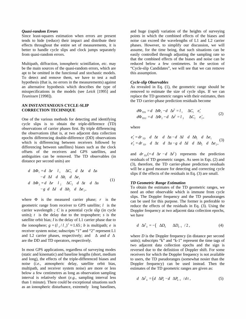
receiver has a millisecond jump about every 10 minutes depending on receiver clock status. Fig. 1 shows the receiver clock bias estimates using the C/A-code pseudoranges already corrected for ± 1 millisecond clock offsets. The effect of geometric range change corresponding to the offset is hidden due to the noise of the code observations. However, the carrier phase observations clearly show such effects in their TD time series (Fig. 2).

Figure 1. Receiver clock bias estimates using C/A-code pseudoranges in stand-alone mode (Ashtech Z-12).

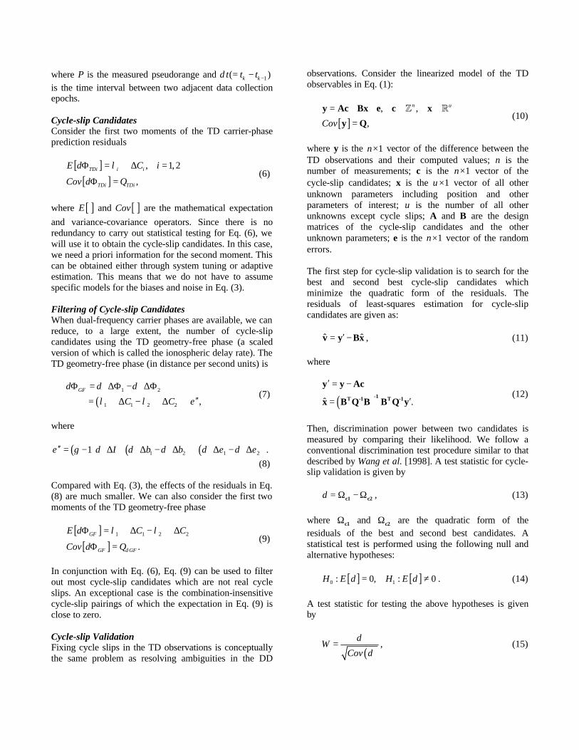
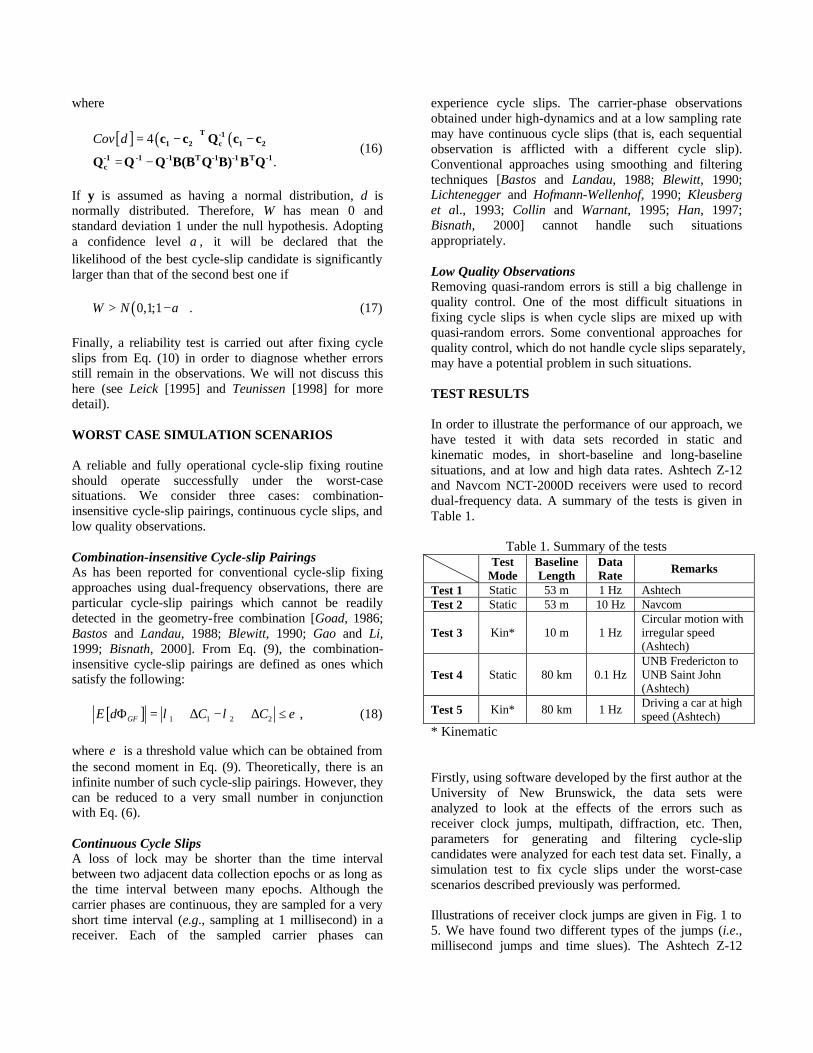
Figure 2. Receiver clock jumps in the TD carrier-phase observations (Ashtech Z-XII). The Navcom NCT-2000D receiver shows very intricate patterns in the clock bias estimates using C/A-code pseudoranges (Fig. 3). The insert shows the clock bias estimates for 10 seconds allowing the clock’s behaviour to be seen in detail. The clock is slued every second. Fig. 4 shows the effects of time slues in the TD carrier-phase measurements.

Figure 3. Receiver clock bias estimates using C/A-code pseudoranges in stand-alone mode (Navcom NCT-2000D).

Figure 4. Receiver clock jumps in the TD carrier-phase observations (Navcom NCT-2000D).

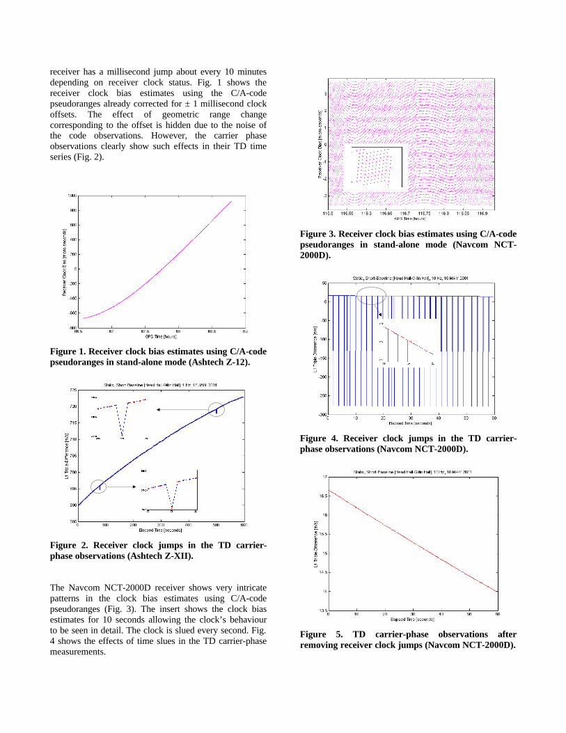
Figure 5. TD carrier-phase observations after removing receiver clock jumps (Navcom NCT-2000D).

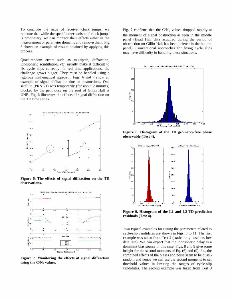
To conclude the issue of receiver clock jumps, we reiterate that while the specific mechanism of clock jumps is proprietary, we can monitor their effects either in the measurement or parameter domains and remove them. Fig. 5 shows an example of results obtained by applying this process. Quasi-random errors such as multipath, diffraction, ionospheric scintillation, etc. usually make it difficult to fix cycle slips correctly. In real-time applications, the challenge grows bigger. They must be handled using a rigorous mathematical approach. Figs. 6 and 7 show an example of signal diffraction due to obstructions. One satellite (PRN 21) was temporarily (for about 2 minutes) blocked by the penthouse on the roof of Gillin Hall at UNB. Fig. 6 illustrates the effects of signal diffraction on the TD time series.

Figure 6. The effects of signal diffraction on the TD observations.

Figure 7. Monitoring the effects of signal diffraction using the C/N0 values.

Fig. 7 confirms that the 0C/N values dropped rapidly at the moment of signal obstruction as seen in the middle panel (Head Hall data acquired during the period of obstruction on Gillin Hall has been deleted in the bottom panel). Conventional approaches for fixing cycle slips may have difficulty in handling these situations.

Figure 8. Histogram of the TD geometry-free phase observable (Test 4).

Figure 9. Histogram of the L1 and L2 TD prediction residuals (Test 4). Two typical examples for tuning the parameters related to cycle-slip candidates are shown in Figs. 8 to 11. The first example was taken from Test 4 (static, long-baseline, low data rate). We can expect that the ionospheric delay is a dominant bias source in this case. Figs. 8 and 9 give some insight for the second moments of Eq. (6) and (9); i.e., the combined effects of the biases and noise seem to be quasi-random and hence we can use the second moments to set threshold values in limiting the ranges of cycle-slip candidates. The second example was taken from Test 3

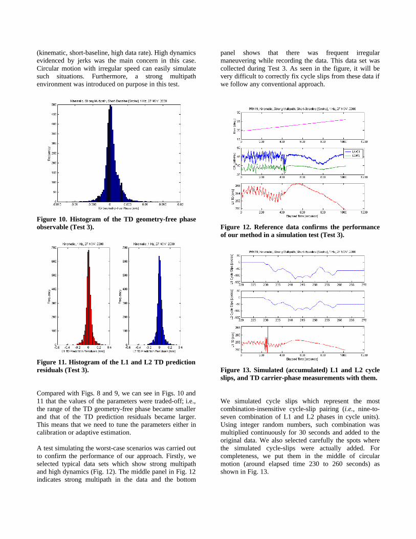
(kinematic, short-baseline, high data rate). High dynamics evidenced by jerks was the main concern in this case. Circular motion with irregular speed can easily simulate such situations. Furthermore, a strong multipath environment was introduced on purpose in this test.

Figure 10. Histogram of the TD geometry-free phase observable (Test 3).

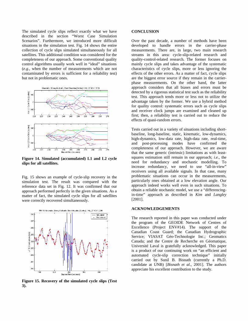
Figure 11. Histogram of the L1 and L2 TD prediction residuals (Test 3). Compared with Figs. 8 and 9, we can see in Figs. 10 and 11 that the values of the parameters were traded-off; i.e., the range of the TD geometry-free phase became smaller and that of the TD prediction residuals became larger. This means that we need to tune the parameters either in calibration or adaptive estimation. A test simulating the worst-case scenarios was carried out to confirm the performance of our approach. Firstly, we selected typical data sets which show strong multipath and high dynamics (Fig. 12). The middle panel in Fig. 12 indicates strong multipath in the data and the bottom

panel shows that there was frequent irregular maneuvering while recording the data. This data set was collected during Test 3. As seen in the figure, it will be very difficult to correctly fix cycle slips from these data if we follow any conventional approach.

Figure 12. Reference data confirms the performance of our method in a simulation test (Test 3).

Figure 13. Simulated (accumulated) L1 and L2 cycle slips, and TD carrier-phase measurements with them. We simulated cycle slips which represent the most combination-insensitive cycle-slip pairing (i.e., nine-to-seven combination of L1 and L2 phases in cycle units). Using integer random numbers, such combination was multiplied continuously for 30 seconds and added to the original data. We also selected carefully the spots where the simulated cycle-slips were actually added. For completeness, we put them in the middle of circular motion (around elapsed time 230 to 260 seconds) as shown in Fig. 13.

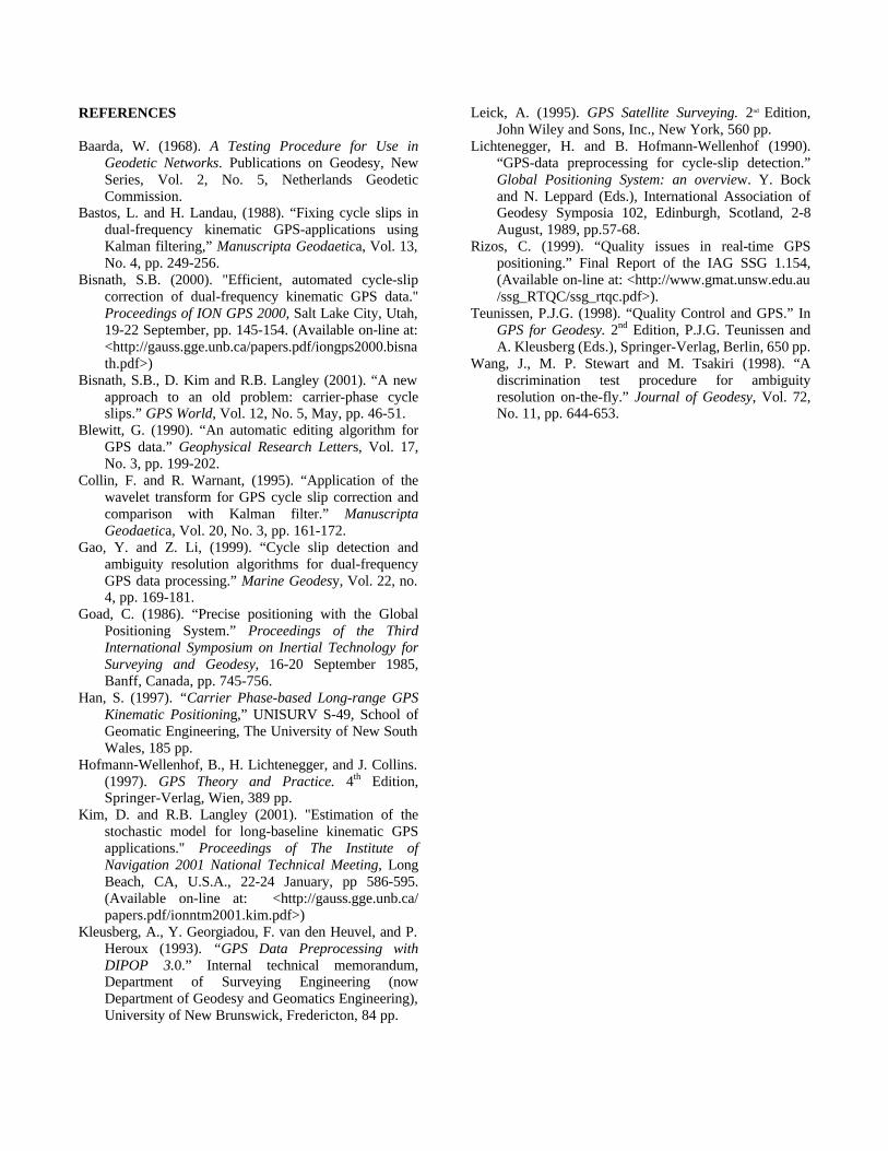
The simulated cycle slips reflect exactly what we have described in the section “Worst Case Simulation Scenarios”. Furthermore, we introduced more difficult situations in the simulation test. Fig. 14 shows the entire collection of cycle slips simulated simultaneously for all satellites. This additional condition was considered for the completeness of our approach. Some conventional quality control algorithms usually work well in “ideal” situations (e.g., when the number of measurements which are not contaminated by errors is sufficient for a reliability test) but not in problematic ones.

Figure 14. Simulated (accumulated) L1 and L2 cycle slips for all satellites. Fig. 15 shows an example of cycle-slip recovery in the simulation test. The result was compared with the reference data set in Fig. 12. It was confirmed that our approach performed perfectly in the given situations. As a matter of fact, the simulated cycle slips for all satellites were correctly recovered simultaneously.

Figure 15. Recovery of the simulated cycle slips (Test 3).

CONCLUSION Over the past decade, a number of methods have been developed to handle errors in the carrier-phase measurements. There are, in large, two main research streams in this area: cycle-slip-related research and quality-control-related research. The former focuses on mainly cycle slips and takes advantage of the systematic characteristics of cycle slips, more or less ignoring the effects of the other errors. As a matter of fact, cycle slips are the biggest error source if they remain in the carrier-phase measurements. On the other hand, the latter approach considers that all biases and errors must be detected by a rigorous statistical test such as the reliability test. This approach tends more or less not to utilize the advantage taken by the former. We use a hybrid method for quality control: systematic errors such as cycle slips and receiver clock jumps are examined and cleaned up first; then, a reliability test is carried out to reduce the effects of quasi-random errors. Tests carried out in a variety of situations including short-baseline, long-baseline, static, kinematic, low-dynamics, high-dynamics, low-data rate, high-data rate, real-time, and post-processing modes have confirmed the completeness of our approach. However, we are aware that the same generic (intrinsic) limitations as with least-squares estimation still remain in our approach; i.e., the need for redundancy and stochastic modelling. To increase redundancy, we need to use “all-in-view” receivers using all available signals. In that case, many problematic situations can occur in the measurements, particularly ones obtained at a low elevation angle. Our approach indeed works well even in such situations. To obtain a reliable stochastic model, we use a “differencing-in-time” approach as described in Kim and Langley [2001]. ACKNOWLEDGEMENTS The research reported in this paper was conducted under the program of the GEOIDE Network of Centres of Excellence (Project ENV#14). The support of the Canadian Coast Guard; the Canadian Hydrographic Service; VIASAT Géo-Technologie Inc.; Geomatics Canada; and the Centre de Recherche en Géomatique, Université Laval is gratefully acknowledged. This paper is a product of our continuing work on “an efficient and automated cycle-slip correction technique” initially carried out by Sunil B. Bisnath (currently a Ph.D. candidate at UNB) [Bisnath et al., 2001]. The authors appreciate his excellent contribution to the study.

REFERENCES Baarda, W. (1968). A Testing Procedure for Use in

Geodetic Networks. Publications on Geodesy, New Series, Vol. 2, No. 5, Netherlands Geodetic Commission.

Bastos, L. and H. Landau, (1988). “Fixing cycle slips in dual-frequency kinematic GPS-applications using Kalman filtering,” Manuscripta Geodaetica, Vol. 13, No. 4, pp. 249-256.

Bisnath, S.B. (2000). "Efficient, automated cycle-slip correction of dual-frequency kinematic GPS data." Proceedings of ION GPS 2000, Salt Lake City, Utah, 19-22 September, pp. 145-154. (Available on-line at: <http://gauss.gge.unb.ca/papers.pdf/iongps2000.bisnath.pdf>)

Bisnath, S.B., D. Kim and R.B. Langley (2001). “A new approach to an old problem: carrier-phase cycle slips.” GPS World, Vol. 12, No. 5, May, pp. 46-51.

Blewitt, G. (1990). “An automatic editing algorithm for GPS data.” Geophysical Research Letters, Vol. 17, No. 3, pp. 199-202.

Collin, F. and R. Warnant, (1995). “Application of the wavelet transform for GPS cycle slip correction and comparison with Kalman filter.” Manuscripta Geodaetica, Vol. 20, No. 3, pp. 161-172.

Gao, Y. and Z. Li, (1999). “Cycle slip detection and ambiguity resolution algorithms for dual-frequency GPS data processing.” Marine Geodesy, Vol. 22, no. 4, pp. 169-181.

Goad, C. (1986). “Precise positioning with the Global Positioning System.” Proceedings of the Third International Symposium on Inertial Technology for Surveying and Geodesy, 16-20 September 1985, Banff, Canada, pp. 745-756.

Han, S. (1997). “Carrier Phase-based Long-range GPS Kinematic Positioning,” UNISURV S-49, School of Geomatic Engineering, The University of New South Wales, 185 pp.

Hofmann-Wellenhof, B., H. Lichtenegger, and J. Collins. (1997). GPS Theory and Practice. 4th Edition, Springer-Verlag, Wien, 389 pp.

Kim, D. and R.B. Langley (2001). "Estimation of the stochastic model for long-baseline kinematic GPS applications." Proceedings of The Institute of Navigation 2001 National Technical Meeting, Long Beach, CA, U.S.A., 22-24 January, pp 586-595. (Available on-line at: <http://gauss.gge.unb.ca/ papers.pdf/ionntm2001.kim.pdf>)

Kleusberg, A., Y. Georgiadou, F. van den Heuvel, and P. Heroux (1993). “GPS Data Preprocessing with DIPOP 3.0.” Internal technical memorandum, Department of Surveying Engineering (now Department of Geodesy and Geomatics Engineering), University of New Brunswick, Fredericton, 84 pp.

Leick, A. (1995). GPS Satellite Surveying. 2nd Edition, John Wiley and Sons, Inc., New York, 560 pp.

Lichtenegger, H. and B. Hofmann-Wellenhof (1990). “GPS-data preprocessing for cycle-slip detection.” Global Positioning System: an overview. Y. Bock and N. Leppard (Eds.), International Association of Geodesy Symposia 102, Edinburgh, Scotland, 2-8 August, 1989, pp.57-68.

Rizos, C. (1999). “Quality issues in real-time GPS positioning.” Final Report of the IAG SSG 1.154, (Available on-line at: <http://www.gmat.unsw.edu.au /ssg_RTQC/ssg_rtqc.pdf>).

Teunissen, P.J.G. (1998). “Quality Control and GPS.” In GPS for Geodesy. 2nd Edition, P.J.G. Teunissen and A. Kleusberg (Eds.), Springer-Verlag, Berlin, 650 pp.

Wang, J., M. P. Stewart and M. Tsakiri (1998). “A discrimination test procedure for ambiguity resolution on-the-fly.” Journal of Geodesy, Vol. 72, No. 11, pp. 644-653.