Biol Cybern (2013) 107:179–200DOI 10.1007/s00422-012-0545-z

ORIGINAL PAPER

Instantaneous kinematic phase reflects neuromechanical responseto lateral perturbations of running cockroaches

Shai Revzen · Samuel A. Burden · Talia Y. Moore ·Jean-Michel Mongeau · Robert J. Full

Received: 19 July 2012 / Accepted: 27 December 2012 / Published online: 1 February 2013© Springer-Verlag Berlin Heidelberg 2013

Abstract Instantaneous kinematic phase calculation allowsthe development of reduced-order oscillator models usefulin generating hypotheses of neuromechanical control. Whenperturbed, changes in instantaneous kinematic phase and fre-quency of rhythmic movements can provide details of move-ment and evidence for neural feedback to a system-levelneural oscillator with a time resolution not possible withtraditional approaches. We elicited an escape response incockroaches (Blaberus discoidalis) that ran onto a movablecart accelerated laterally with respect to the animals’ motioncausing a perturbation. The specific impulse imposed on ani-mals (0.50 ± 0.04 m s−1; mean, SD) was nearly twice theirforward speed (0.25 ± 0.06 m s−1). Instantaneous residualphase computed from kinematic phase remained constant for110 ms after the onset of perturbation, but then decreasedrepresenting a decrease in stride frequency. Results fromdirect muscle action potential recordings supported kine-matic phase results in showing that recovery begins with self-stabilizing mechanical feedback followed by neural feedbackto an abstracted neural oscillator or central pattern generator.Trials fell into two classes of forward velocity changes, whileexhibiting statistically indistinguishable frequency changes.Animals pulled away from the side with front and hind legsof the tripod in stance recovered heading within 300 ms,

S. Revzen · T. Y. Moore · R. J. Full (B)Department of Integrative Biology, University of California,Berkeley, CA 94720, USAe-mail: rjfull@berkeley.edu

S. A. BurdenDepartment of Electrical Engineering and Computer Sciences,University of California, Berkeley, CA 94720, USA

J.-M. MongeauBiophysics Graduate Group, University of California, Berkeley, CA94720, USA

whereas animals that only had a middle leg of the tripodresisting the pull did not recover within this period. Animalswith eight or more legs might be more robust to lateral per-turbations than hexapods.

Keywords Biomechanics · Phase · Neuromechanicalcontrol · Neural clock · Locomotion · Cockroach ·Perturbation

Abbreviations

Axes Y -axis is positive along the line of platformtranslation. Also called lateral axis. Z-axisis perpendicular to the Y -axis, positive ver-tical of the platform. X-axis is perpendicularto both the Y - and Z-axes, and positive inthe direction of cockroach locomotion. Alsocalled the forward axis

Vx Component of cockroach velocity in track-way direction

Vy Component of cockroach velocity acrosstrackway

COM Center of massCPG Central pattern generator

EMG ElectromyographyIBI Inter-burst interval. The time between two

bursts of muscle action potentials in an elec-tromyography

ISI Inter-spike intervalLLS Lateral leg spring model

MAP Muscle action potentialPCA Principal component analysisLLS Lateral leg spring model

123

180 Biol Cybern (2013) 107:179–200

AEP Anterior extreme position. The transitionfrom swing to stance.

PEP Posterior extreme position. The transitionfrom stance to swing.

SLIP Spring loaded inverted pendulum model

List of symbols

Φ Phase threshold between classes (oneclass has Φ − π < φ0 < Φ, the otherΦ < φ0 < Φ + π )

φ0 Predictor phaseφ, θ Phases

ω Derivative of phase with respect to time,i.e. instantaneous frequency

�φ Residual phasex, v Position, velocity time series used to cre-

ate complex phase time seriesz Complex phase time series 〈.〉 mean

value; 〈w(t)〉 is the expectation of thevariable w(t)

t1pre Starting time window pre-perturbationt2pre Ending time window pre-perturbationtstep Step duration

ton Onset of perturbationt1post Starting time window post-perturbationt2post Ending time window post-perturbation

std Standard deviation operator; std[w(t)] isthe standard deviation of the variablew(t)

exp (Complex) exponential functionarg Complex argument (i.e., polar angle)

functionC0 Class 0, one of the two phase classes (in

red)C1 Class 1, one of the two phase classes (in

blue)Vx0 Mean of cockroach velocity in trackway

direction for C0

Vx1 Mean of cockroach velocity in trackwaydirection for C1

L1 norm Sum of absolute differencesL2 norm Square root of sum of squared differ-

ences, same as root mean square (RMS)up to a scale

N Parameter governing the number of boot-strap trials used for testing classificationsignificance; N 2 trials for H1 and H0(a)

are compared with a nested bootstrap ofN trials of N nested trials each.

n Number of trials provided by an individ-ual animal

H1 Statistical hypothesis that classes the C0

and C1 obtained from φ0 and Φ describeanimals that behave differently.

H0(a) Statistical hypothesis that trial classes C0

and C1 are selected at random from thesame distribution of animal motions.

H0(b) Statistical hypothesis that trial classes C0

and C1 are selected to be most dissimi-lar classes that can be obtained based ona choice of Φ, while still being selectedat random from the same distribution ofanimal motions.

χ2 Statistical distribution and associated test

1 Introduction

Using the rhythmic motion of diverse body structures andappendages, animals adopt a wide spectrum of locomotorbehaviors to move through every variety of natural environ-ments. As they move, animals must respond to unexpectedperturbations such as changes in terrain, injury to limbs, andthe behavior of predators, prey, and conspecifics. We pro-pose that within the kinematic responses to these perturba-tions reside patterns revealing the interplay between neuraland mechanical stabilization that govern the recovery fromperturbation. Using the instantaneous phase and frequencyof rhythmic limb movements, Revzen et al. [2008] offer ageneral framework for identifying which candidate feedbackpathways within neuromechanical control architectures playthe dominant role in coordinating neuromechanical oscilla-tions (Fig. 1).

1.1 Neuromechanical control architectures

With the simplest neuromechanical control architectures pos-sible, at least three types of feedback pathways contribute tostabilization. Figure 1A corresponds to a hypothesis basedprimarily on mechanical stabilization, Fig. 1B on time-invariant (classical) reflex feedback, and Fig. 1C on feed-back modulation of the entire gait pattern. The overall frame-work of neuromechanical control in which we ground thesehypotheses assumes that motions are driven by endogenouslyproduced rhythmic pattern oscillations emitted from a CPG(Delcomyn 1980; Büschges 2005; Büschges et al. 2011;Marder et al. 2005; Grillner 1985; MacKay-Lyons 2002). Forthe running behavior described here, we use CPG to repre-sent a reduced-order, system-level model composed of mul-tiple interacting neural CPG circuits that are phase-locked(Revzen et al. 2008; Revzen 2009; Fuchs et al. 2011, 2012).The CPG is coupled to an oscillating mechanical systemcomposed of appendages, skeleton and the muscles that con-nect them. In turn, this mechanical system is coupled to theenvironment.

123

Biol Cybern (2013) 107:179–200 181

A B C

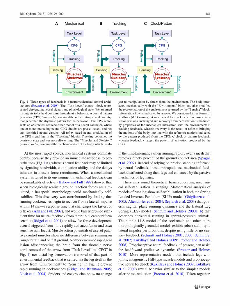
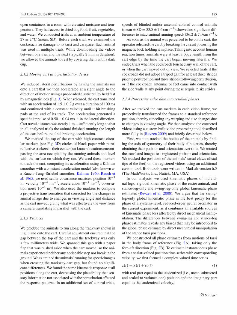
Fig. 1 Three types of feedback in a neuromechanical control archi-tectures (Revzen et al. 2008). The “Task Level” control block repre-sented descending neural signals and physiological state. We assumedits outputs to be held constant throughout a behavior. A central patterngenerator (CPG, blue circle) contained the self-exciting neural circuitrythat generated the rhythmic pattern for the behavior. Here CPG repre-sents an abstracted, reduced-order model of a neural oscillator, whereone or more interacting neural CPG circuits are phase-locked, and notany identified neural circuits. All reflex-based neural modulation ofthe CPG signal lay in the “Tracking” blocks. Tracking contained nopersistent state and was not self-exciting. The “Muscles and Skeleton”(nested circles) contained the mechanical state of the body, which is sub-

ject to manipulation by forces from the environment. The body inter-acted mechanically with the “Environment” block and also modifiedthe representation of the environment returned by the “Sensing” block.Information flow is indicated by arrows. We considered three forms offeedback (thick arrows): A mechanical feedback, wherein muscle acti-vation remains unchanged and recovery from perturbation is mediatedby properties of the mechanical interaction with the environment; Btracking feedback, wherein recovery is the result of reflexes bringingthe motions of the body into line with the reference motions indicatedby the pattern produced from the CPG; C clock or pattern feedback,wherein feedback changes the pattern of activation produced by theCPG

At the most rapid speeds, mechanical systems dominatecontrol because they provide an immediate response to per-turbations (Fig. 1A), whereas neural feedback may be limitedby signaling bandwidth, computation ability, and the delaysinherent in muscle force recruitment. When a mechanicalsystem is tuned to its environment, mechanical feedback canbe remarkably effective. (Kubow and Full 1999) showed thatwhen biologically realistic ground reaction forces are sim-ulated, a hexapedal morphology could mechanically self-stabilize. This discovery was corroborated by finding thatrunning cockroaches begin to recover from a lateral impulsewithin 14 ms—a response time that challenges the fastest ofreflexes (Ahn and Full 2002), and would barely provide suffi-cient time for neural feedback from their tibial campaniformsensilla (Ridgel et al. 2001) or allow for force developmenteven if triggered from more rapidly activated femur and coxasensillae as in locust. Muscle action potentials of a set of puta-tive control muscles show no difference between running onrough terrain and on flat ground. Neither circumoesophageallesion (disconnecting the brain from the thoracic nervecord; removal of the arrow from “Task Level” to “CPG” inFig. 1) nor distal leg denervation (removal of that part ofenvironmental feedback that is sensed via the leg itself in thearrow from “Environment” to “Sensing” in Fig. 1) preventrapid running in cockroaches (Ridgel and Ritzmann 2005;Noah et al. 2004). Spiders and cockroaches show no change

in the limb kinematics when running rapidly over a mesh thatremoves ninety percent of the ground contact area (Spagnaet al. 2007). Instead of relying on precise stepping informedby neural feedback, these arthropods use mechanical feed-back distributed along their legs and enhanced by the passivemechanics of leg hairs.

There is a sound theoretical basis supporting mechani-cal self-stabilization in running. Mathematical analysis ofmodels of running show self-stabilization in both the SpringLoaded Inverted Pendulum (SLIP) model (Ghigliazza et al.2005; Altendorfer et al. 2004; Seyfarth et al. 2003) that gov-erns sagittal plane running dynamics and the Lateral LegSpring (LLS) model (Schmitt and Holmes 2000a, b) thatdescribes horizontal running in sprawl-postured animals.The simple LLS model of the cockroach and other moremorphologically grounded models exhibit robust stability tolateral impulse perturbations, despite using little or no sen-sory feedback (Schmitt and Holmes 2001, 2003; Schmitt etal. 2002; Kukillaya and Holmes 2009; Proctor and Holmes2008). Proprioceptive neural feedback, if present, can assistthe feedfoward preflexive dynamics (Proctor and Holmes2010). More representative models that include legs withjoints, antagonistic Hill-type muscle models and propriocep-tive neural feedback (Kukillaya and Holmes 2009; Kukillayaet al. 2009) reveal behavior similar to the simpler modelsafter phase-reduction (Proctor et al. 2010). Taken together,

123

182 Biol Cybern (2013) 107:179–200

the combination of theoretical plausibility and empirical evi-dence provides a strong case for mechanical self-stabilizationduring high-speed running (Holmes et al. 2006).

At slower speeds and for more precise movements, neuralfeedback from sensors (Fig. 1B) is the dominant modality ofcontrol. The important role of neural reflexes in slow loco-motion is well established in insects. For the slow, quasi-static locomotion of stick insects, the artificial neural net“WalkNet” provides an effective representation of control(Cruse and Schwarze 1988; Cruse and Knauth 1989; Cruseet al. 2007; Schilling et al. 2007) that includes targeted footplacement mediated by feedback. The model is largely kine-matic in nature because inertia and momentum play almostno role in slow walking (Klavins et al. 2002). Even inslow running insects, sensors associated with neural reflexesrespond to environmental perturbations by feeding back onthe patterns emitted by a CPG (Ijspeert 2008; Ritzmannand Büschges 2007; Fig. 1B symbolized by the “Tracking”block).

A large body of research has shown that the neural reflexescontrolling locomotion are far richer in behavior than ourtypical view of a stereotyped, negative feedback loop (e.g.,Pearson 1995, 2004). For example, load compensating reac-tions in land mammals and arthropods depend on the type ofsensor (sensing self vs. environment), the preparation stud-ied (intact vs. isolated), the task (immobile, walking vs. run-ning), the intensity of muscle contraction, the phase in thegait (swing vs. stance), and the relative importance of pas-sive versus reflexive stiffness (Duysens et al. 2000; Zehr andStein 1999). Some mammalian reflexes that provide nega-tive force feedback gains under most circumstances providepositive gains during locomotion, increasing force produc-tion during stance (Prochazka et al. 1997a, b; Pearson andCollins 1993). Sensory information may introduce coordina-tion and adaptation of locomotor patterns that would other-wise be independent and unmodulated (Grillner and Wallén2002), or it may be critically necessary for oscillations toappear at all (Pearson 1993, 1995, 2004).

We place locomotor neural reflexes regardless of whetherthey were triggered by proprioceptive or exteroceptive sens-ing into two broad categories—one that affects the outputof the CPG (Tracking; Fig. 1B) and the other that alters therhythm of the CPG itself (Fig. 1C). One may envision track-ing feedback to be a means of matching a limb’s motionto an implied reference motion generated by the CPG andcan be characterized as following an equilibrium-point tra-jectory (Jaric and Latash 2000). Mathematically, trackingis time-invariant, stateless (has no memory of past inputs),and functions by comparing the actual state of the body tothe reference provided by the CPG, then generating forceactivation in muscles. Tracking contains no persistent stateand is not self-exciting. Feedback via such tracking reflexes(Fig. 1B) does not modulate the rhythm emitted by the CPG.

In the Fig. 1C category, we define neural feedback that doesalter the rhythm from the CPG. Neural feedback in this cat-egory could result in changes in the frequency output by theCPG.

1.2 Kinematic phase can reflect feedback to thesystems-level CPG

In Revzen et al. [2008], we proposed methods for identify-ing the interplay of neural and mechanical feedback by prob-ing rhythmic behaviors through computing phase estimatesderived from kinematic observations—a “kinematic phase”.Examination of kinematic phase can illuminate the couplingbetween the mechanical oscillator—the body, muscle, andskeleton—and the neural oscillator(s) (CPG(s)) that drives it(Fig. 1). When an animal is engaged in a rhythmic behav-ior, all the subsystems involved in producing that behaviorand all observable quantities describing those subsystemswill oscillate rhythmically. The implication for experimen-tal biomechanics is that the kinematics of the body and itssubsystems must reflect the underlying oscillator state.

The advantage of the kinematic phase method (Revzen andGuckenheimer 2008) is that for animal locomotion with sta-ble oscillations, phase provides a quantitative and predictivemodel of movement. When given the readily measured kine-matic state of the animal in as little as two consecutive framesof video, one can compute the phase and frequency, extrap-olate the linear relationship of phase to time, and predict thekinematic states at all future times. In practice, because ani-mals are continuously perturbed from the idealized dynamicsof the template (Full and Koditschek 1999), the accuracy ofprediction diminishes over time and requires frequency esti-mates over more than just a pair of frames. Nevertheless, theability to take a dataset only a fraction of a step long, obtainphase and frequency, and project anticipated kinematics sev-eral strides into the future provides a powerful means for test-ing perturbation recovery against an unperturbed alternative.

For constant frequency locomotion such as running, theanimal’s motions will over time settle to a constant phase rel-ative to the timing of the signal emitted by the systems-level,synchronized CPG. This phenomenon is known as “phaselocking” or “entrainment”. We may thus postulate that thepre-perturbation animal is an entrained neural and mechani-cal oscillator. Relative to time, the kinematic phase of such ananimal would follow a linear model with running frequencybeing the slope of a phase versus time plot. Due to entrain-ment, the kinematic phase must be at a constant phase offsetrelative to the phase of the systems-level CPG.

When the animal is perturbed, some transient responseappears and decays, and the animal resumes running at a con-stant, but possibly different, frequency. We propose to detectchanges in phase by fitting a linear regression model to pre-perturbation phase data and extrapolating an expected phase

123

Biol Cybern (2013) 107:179–200 183

past the perturbation and into the recovery phase. Subtract-ing that estimate from the post-perturbation kinematic phase,we will provide a “residual phase” succinctly expressing anychanges in the animal’s rhythm and timing of movement.

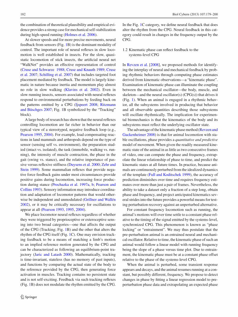
Figure 2A–D, derived from (Revzen et al. 2008), showsthe procedure of going from leg kinematics to residual phaseusing experimental data from a hexapedal runner experienc-ing a perturbation. The position data represent the fore-aft legmotions relative to the body as a function of time. Theoret-ically possible outcomes of the perturbation experiment arerepresented with simulated data in Fig. 2E–G. In Fig. 2F, weshow the linear model extrapolations for position and resid-ual phase post-perturbation (i.e., gray lines). Differences inthe slope of the linear models (Fig. 2G) indicate changes inrunning frequency, and can only persist if the neural signaldriving the muscles changes frequency as well. Thus, if wesee no residual phase change after a perturbation (Fig. 2E),we hypothesize that the most parsimonious neural controlarchitecture characterizing the response is one that involvesmechanical feedback (Fig. 1A). If the perturbation causesa change in the systems-level CPG frequency, as seen inFig. 2G, we reject the possibility of the mechanical feedbackpathway (Fig. 1A) and the tracking neural feedback pathway(Fig. 1B) in favor of the control architecture sending neuralfeedback to the systems-level CPG (Fig. 1C). Phase changeoutcomes (Fig. 2F) can appear in all three feedback archi-tectures (Fig. 1), but can be further analyzed based on theirsensitivity to perturbation magnitudes.

1.3 Model system testing the utility of kinematic phase

The best candidates to test neuromechanical control hypothe-ses using kinematic phase are animals whose anchored mor-phology expresses the rhythmic motions of the templatewith many easily measurable appendages. These animalswould expose a great deal of phase information through theirkinematics, making kinematic phase a reliable estimate oftheir overall phase. Here, we test these hypotheses using ahexapedal runner, the cockroach Blaberus discoidalis, notonly because of the phase data offered by six oscillating legs,but because few species have as extensive a biomechanical(Kram et al. 1997; Full et al. 1991; Full and Tu 1990; Tinget al. 1994; Jindrich and Full 1999; Ahn et al. 2006; Ahnand Full 2002) and neurophysiological (Watson and Ritz-mann 1998a, b; Watson et al. 2002a, b; Zill et al. 1981, 2004,2009) characterization.

In this study, we used kinematic phase (Revzen and Guck-enheimer 2008) to investigate the time-course of cockroachrecovery from a lateral impulse perturbation. The perturba-tions occurred when the animals were running at interme-diate speeds, where the likelihood of viewing the interplaybetween neural and mechanical feedback was the greatest.By comparing instantaneous residual phase before and after

the perturbation (Fig. 2), we could propose when mechanicalfeedback was sufficient, neural feedback must be used, or asensory signal was sent to modulate the abstracted, systems-level CPG (Fig. 1). Because we measured leg kinematics, wecould explore the relationship of an animal’s posture and itsmechanical response to its control strategy.

To test whether instantaneous kinematic phase at the sys-tems level reflects neuromechanical feedback in well-studiedleg control muscles (Sponberg et al. 2011a, b, Sponbergand Full 2008; Ahn and Full 2002; Ahn et al. 2006; Fullet al. 1998), we recorded muscle action potentials (MAPs)from femoral extensors 178 and 179. We selected these mus-cles because their single fast motor neuron innervation (Df)

allows the simplest possible characterization of activation(Pearson and Iles 1971). Moreover, Sponberg and Full [2008]found no significant difference in the inter-spike interval,burst phase or inter-burst period between flat and very roughterrain suggesting a greater contribution of mechanical feed-back. By contrast, during the largest perturbations, neuralfeedback was detectable as a phase shift of the central rhythm.In this key control muscle, we hypothesize that the lack ofchange in instantaneous kinematic phase will be associatedwith no change in MAP inter-burst periods, supporting apossible greater reliance on mechanical feedback, whereas achange in kinematic phase will coincide with a concomitantchange in MAP inter-burst periods reflecting neural feedback

2 Lateral perturbation experiment

We ran cockroaches onto a perturbation device consistingof a rail-mounted cart that was accelerated horizontally bya manually keyed mechanism. In the reference frame of thecart, the cockroach center-of-mass received a large lateralimpulse perpendicular to its heading. We recorded the trialsusing an overhead high-speed video camera and digitized themotions of the cockroach feet (tarsi). By applying methodsdeveloped in Revzen et al. [2008] and Revzen and Guck-enheimer [2008] and used in Revzen [2009] Chapter 2, weused the tarsal trajectories in the body frame of reference toestimate the kinematic phase of the animals, and then fit aconstant frequency model to the pre-perturbation phase datausing linear regression. We used the residual phases derivedfrom these regression models to test our neuromechanicalhypotheses.

2.1 Lateral perturbation kinematics

2.1.1 Animals

We obtained the fifteen B. discoidalis cockroaches used inthis study from a commercial supplier (Carolina BiologicalSupply Co., Gladstone, OR, USA) and kept them in large,

123

184 Biol Cybern (2013) 107:179–200

A

D

E

F

G

B C

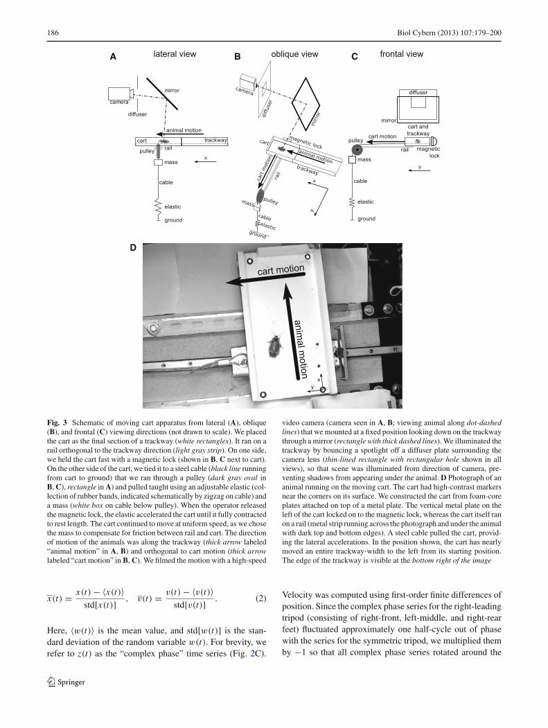
Fig. 2 From kinematics to kinematic phase. (A–D from typicalanimal trial) A Foot or tarsus trajectories over 1.1 s, in bodycoordinates, and fore-aft tarsus positions plotted over time (B).Lower plot in B indicates cart lateral acceleration (1 g scale barshown at t = 0), with vertical lines indicating peak (thick line,0.5 g thin lines) of perturbation which starts at t = 0. The complex-valued phase of the left hind leg (leg 3, red in A, B) is shown (C,dashed blue) together with the swing-only complex-valued phase, inwhich stances are linearly interpolated in complex argument and mag-nitude (C, solid red). The resulting residual phase for times–100 to300 ms is shown in D, with corresponding times indicated by verticallines in B. Theoretically plausible residual phase outcomes for per-turbation experiments showing both (simulated) fore-aft leg positionsover time on the left (E–G), next to the corresponding residual phaseplot on the right. In E, we show an animal that slowed down dur-

ing perturbation, but fully recovered to motions matching the motionsextrapolated from pre-perturbation motion (solid red fitting region forregression model, dashed red line extrapolated model, solid green post-perturbation regression); this can be interpreted as the perturbation hav-ing broken the entrainment of body to system-level neural CPG, andthat entrainment re-establishing itself post-perturbation. It is compati-ble with both Fig. 1A, B feedback alternatives. In F, we show an animalthat recovers the same frequency at a phase offset; this can be inter-preted as the re-entrainment locking on to a different stable relation-ship between the neural and mechanical oscillations, and is similarlycompatible with Fig. 1A, B. In G, we show an animal whose frequencychanges, as expressed by the non-zero slope of the residual phase trend-line; such a change requires the system-level CPG to change frequency,and is therefore only compatible with the Fig. 1C feedback to the system-level CPG

123

Biol Cybern (2013) 107:179–200 185

open containers in a room with elevated moisture and tem-perature. They had access to dried dog food, fruit, vegetables,and water. We conducted trials at an ambient temperature of27 ± 2 ◦C (mean, SD). Before each trial, we examined thecockroach for damage to its tarsi and carapace. Each animalwas used in multiple trials. While downloading the videosbetween one trial and the next (typically 2 min in duration),we allowed the animals to rest by covering them with a darkcup.

2.1.2 Moving cart as a perturbation device

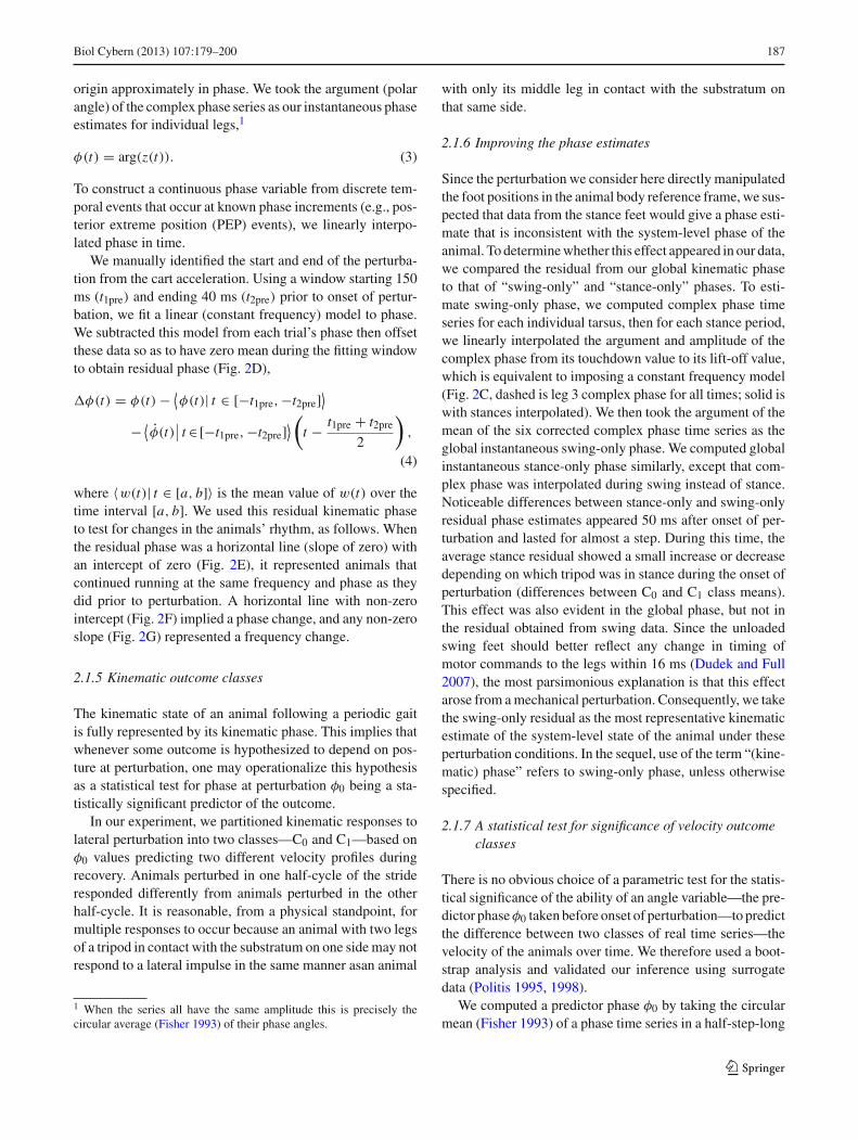
We induced lateral perturbations by having the animals runonto a cart that we then accelerated at a right angle to thedirection of motion using a pre-loaded elastic pulley held fastby a magnetic lock (Fig. 3). When released, the cart translatedwith an acceleration of 1.5 ± 0.2 g over a duration of 100 msand continued with a constant velocity until it hit breakingpads at the end of its track. The acceleration generated aspecific impulse of 0.50 ± 0.04 ms−1 in the lateral direction.Cart travel distance was nearly 1 m—sufficiently long so thatin all analyzed trials the animal finished running the lengthof the cart before the final braking deceleration.

We marked the top of the cart with high-contrast circu-lar markers (see Fig. 3D; circles of black paper with retro-reflective stickers in their centers) at known locations encom-passing the area occupied by the running animals and levelwith the surface on which they ran. We used these markersto track the cart, computing its acceleration using a Kalmansmoother with a constant acceleration model (also known asa Rauch–Tung–Striebel smoother; Kalman 1960, Rauch etal. 1965; we used scalar covariance matrices, position 10−3

m, velocity 10−4 ms−1, acceleration 10−5 ms−2, observa-tion noise 10−2 m). We also used the markers to computea projective transformation that corrected for the changes inanimal image due to changes in viewing angle and distanceas the cart moved, giving what was effectively the view froma camera translating in parallel with the cart.

2.1.3 Protocol

We prodded the animals to run along the trackway shown inFig. 3 and onto the cart. Careful adjustment ensured that thegap between the top of the cart and the trackway was onlya few millimeters wide. We spanned this gap with a paperflap that was pushed aside when the cart moved, so the ani-mals experienced neither any noticeable step nor break in theground. We examined the animals’ running for speed changeswhen crossing the trackway-cart gap, but found no signifi-cant differences. We found the same kinematic response at allpositions along the cart, decreasing the plausibility that sen-sory information not associated with the perturbation affectedthe response patterns. In an additional set of control trials,

speeds of blinded and/or antennal-ablated control animals(mean ± SD = 33.5 ± 7.6 cm s−1) showed no significant dif-ferences to intact animal running speeds (36.2 ± 7.0 cm s−1).

As soon as the animal was perceived to be on the cart, theoperator released the cart by breaking the circuit powering themagnetic lock holding it in place. Taking into account humanreaction times, animals were at least a body length from thecart edge by the time the cart began moving laterally. Weended trials when the cockroach touched any wall of the cart,or when the cart moved out of view. We rejected trials if thecockroach did not adopt a tripod gait for at least three stridesprior to perturbation and three strides following perturbation,or if the cockroach antennae or feet came into contact withthe side walls at any point during these requisite six strides.

2.1.4 Processing video data into residual phases

After we tracked the cart markers in each video frame, weprojectively transformed the frames to a standard referenceposition, thereby canceling any warping and size changes dueto changes in viewing angle. We then analyzed the correctedvideos using a custom built video processing tool describedmore fully in (Revzen 2009) and briefly described below.

First, we auto-tracked the bodies of the animals by find-ing the axis of symmetry of their body silhouettes, therebyobtaining their position and orientation over time. We rotatedthe translated images to a registered position and orientation.We tracked the positions of the animals’ tarsal claws (distaltips of the feet) on the registered videos using an additionalcustom tool. Both tools were written in MatLab version 6.5(The MathWorks, Inc., Natick, MA, USA).

In our analysis, we used kinematic phases of individ-ual legs, a global kinematic phase of the entire animal, andstance-leg-only and swing-leg-only global kinematic phaseestimates (Revzen et al. 2008). We argue that the swing-leg-only global kinematic phase is the best proxy for thephase of a systems-level, reduced-order neural oscillator inthe current experiment, as it combines all available sourcesof kinematic phase less affected by direct mechanical manip-ulation. The differences between swing-leg and stance-legphase estimates reveals any biases that may be introduced tothe global phase estimate by direct mechanical manipulationof the stance tarsi positions.

We constructed all phase estimates from motions of tarsiin the body frame of reference (Fig. 2A), taking only thefore-aft direction (Fig. 2B). To estimate instantaneous phasefrom a scalar-valued position time series with correspondingvelocity, we first formed a complex-valued time series

z(t) = x(t) + iv(t) (1)

with real part equal to the studentized (i.e., mean subtractedand scaled to variance one) position and the imaginary partequal to the studentized velocity,

123

186 Biol Cybern (2013) 107:179–200

A B C

D

Fig. 3 Schematic of moving cart apparatus from lateral (A), oblique(B), and frontal (C) viewing directions (not drawn to scale). We placedthe cart as the final section of a trackway (white rectangles). It ran on arail orthogonal to the trackway direction (light gray strip). On one side,we held the cart fast with a magnetic lock (shown in B, C next to cart).On the other side of the cart, we tied it to a steel cable (black line runningfrom cart to ground) that we ran through a pulley (dark gray oval inB, C), rectangle in A) and pulled taught using an adjustable elastic (col-lection of rubber bands, indicated schematically by zigzag on cable) anda mass (white box on cable below pulley). When the operator releasedthe magnetic lock, the elastic accelerated the cart until it fully contractedto rest length. The cart continued to move at uniform speed, as we chosethe mass to compensate for friction between rail and cart. The directionof motion of the animals was along the trackway (thick arrow labeled“animal motion” in A, B) and orthogonal to cart motion (thick arrowlabeled “cart motion” in B, C). We filmed the motion with a high-speed

video camera (camera seen in A, B; viewing animal along dot-dashedlines) that we mounted at a fixed position looking down on the trackwaythrough a mirror (rectangle with thick dashed lines). We illuminated thetrackway by bouncing a spotlight off a diffuser plate surrounding thecamera lens (thin-lined rectangle with rectangular hole shown in allviews), so that scene was illuminated from direction of camera, pre-venting shadows from appearing under the animal. D Photograph of ananimal running on the moving cart. The cart had high-contrast markersnear the corners on its surface. We constructed the cart from foam-coreplates attached on top of a metal plate. The vertical metal plate on theleft of the cart locked on to the magnetic lock, whereas the cart itself ranon a rail (metal strip running across the photograph and under the animalwith dark top and bottom edges). A steel cable pulled the cart, provid-ing the lateral accelerations. In the position shown, the cart has nearlymoved an entire trackway-width to the left from its starting position.The edge of the trackway is visible at the bottom right of the image

x(t) = x(t) − 〈x(t)〉std[x(t)] , v(t) = v(t) − 〈v(t)〉

std[v(t)] . (2)

Here, 〈w(t)〉 is the mean value, and std[w(t)] is the stan-dard deviation of the random variable w(t). For brevity, werefer to z(t) as the “complex phase” time series (Fig. 2C).

Velocity was computed using first-order finite differences ofposition. Since the complex phase series for the right-leadingtripod (consisting of right-front, left-middle, and right-rearfeet) fluctuated approximately one half-cycle out of phasewith the series for the symmetric tripod, we multiplied themby −1 so that all complex phase series rotated around the

123

Biol Cybern (2013) 107:179–200 187

origin approximately in phase. We took the argument (polarangle) of the complex phase series as our instantaneous phaseestimates for individual legs,1

φ(t) = arg(z(t)). (3)

To construct a continuous phase variable from discrete tem-poral events that occur at known phase increments (e.g., pos-terior extreme position (PEP) events), we linearly interpo-lated phase in time.

We manually identified the start and end of the perturba-tion from the cart acceleration. Using a window starting 150ms (t1pre) and ending 40 ms (t2pre) prior to onset of pertur-bation, we fit a linear (constant frequency) model to phase.We subtracted this model from each trial’s phase then offsetthese data so as to have zero mean during the fitting windowto obtain residual phase (Fig. 2D),

�φ(t) = φ(t) − ⟨φ(t)| t ∈ [−t1pre,−t2pre]

⟩

− ⟨φ̇(t)

∣∣ t ∈[−t1pre,−t2pre]⟩ (

t − t1pre + t2pre

2

),

(4)

where 〈w(t)| t ∈ [a, b]〉 is the mean value of w(t) over thetime interval [a, b]. We used this residual kinematic phaseto test for changes in the animals’ rhythm, as follows. Whenthe residual phase was a horizontal line (slope of zero) withan intercept of zero (Fig. 2E), it represented animals thatcontinued running at the same frequency and phase as theydid prior to perturbation. A horizontal line with non-zerointercept (Fig. 2F) implied a phase change, and any non-zeroslope (Fig. 2G) represented a frequency change.

2.1.5 Kinematic outcome classes

The kinematic state of an animal following a periodic gaitis fully represented by its kinematic phase. This implies thatwhenever some outcome is hypothesized to depend on pos-ture at perturbation, one may operationalize this hypothesisas a statistical test for phase at perturbation φ0 being a sta-tistically significant predictor of the outcome.

In our experiment, we partitioned kinematic responses tolateral perturbation into two classes—C0 and C1—based onφ0 values predicting two different velocity profiles duringrecovery. Animals perturbed in one half-cycle of the strideresponded differently from animals perturbed in the otherhalf-cycle. It is reasonable, from a physical standpoint, formultiple responses to occur because an animal with two legsof a tripod in contact with the substratum on one side may notrespond to a lateral impulse in the same manner asan animal

1 When the series all have the same amplitude this is precisely thecircular average (Fisher 1993) of their phase angles.

with only its middle leg in contact with the substratum onthat same side.

2.1.6 Improving the phase estimates

Since the perturbation we consider here directly manipulatedthe foot positions in the animal body reference frame, we sus-pected that data from the stance feet would give a phase esti-mate that is inconsistent with the system-level phase of theanimal. To determine whether this effect appeared in our data,we compared the residual from our global kinematic phaseto that of “swing-only” and “stance-only” phases. To esti-mate swing-only phase, we computed complex phase timeseries for each individual tarsus, then for each stance period,we linearly interpolated the argument and amplitude of thecomplex phase from its touchdown value to its lift-off value,which is equivalent to imposing a constant frequency model(Fig. 2C, dashed is leg 3 complex phase for all times; solid iswith stances interpolated). We then took the argument of themean of the six corrected complex phase time series as theglobal instantaneous swing-only phase. We computed globalinstantaneous stance-only phase similarly, except that com-plex phase was interpolated during swing instead of stance.Noticeable differences between stance-only and swing-onlyresidual phase estimates appeared 50 ms after onset of per-turbation and lasted for almost a step. During this time, theaverage stance residual showed a small increase or decreasedepending on which tripod was in stance during the onset ofperturbation (differences between C0 and C1 class means).This effect was also evident in the global phase, but not inthe residual obtained from swing data. Since the unloadedswing feet should better reflect any change in timing ofmotor commands to the legs within 16 ms (Dudek and Full2007), the most parsimonious explanation is that this effectarose from a mechanical perturbation. Consequently, we takethe swing-only residual as the most representative kinematicestimate of the system-level state of the animal under theseperturbation conditions. In the sequel, use of the term “(kine-matic) phase” refers to swing-only phase, unless otherwisespecified.

2.1.7 A statistical test for significance of velocity outcomeclasses

There is no obvious choice of a parametric test for the statis-tical significance of the ability of an angle variable—the pre-dictor phase φ0 taken before onset of perturbation—to predictthe difference between two classes of real time series—thevelocity of the animals over time. We therefore used a boot-strap analysis and validated our inference using surrogatedata (Politis 1995, 1998).

We computed a predictor phase φ0 by taking the circularmean (Fisher 1993) of a phase time series in a half-step-long

123

188 Biol Cybern (2013) 107:179–200

(22 ms; 1/2 tstep) window ending at onset of perturbation(ton),

φ0 = arg

(⟨exp(iφ(t))| t ∈ [ton − 1

2tstep, ton]

⟩), (5)

where exp(iφ) is the complex exponential of the imaginaryquantity iφ. Our prediction classified trials into one of twoclasses C0 and C1based on the sign of sin( φ0 −Φ) for someoptimally selected choice of Φ, thereby partitioning the cir-cle of possible phase values into halves with the transitionbetween classes occurring at phases Φ and Φ + π .

We assessed the quality of a classification of trials into C0

and C1 using the root mean squared (or L2 norm) differencebetween the class means of the forward velocity time series(Vx) in a time interval starting 50 ms (t1post) and ending 150ms (t2post) after onset of perturbation. That is, with Vx0 anddenoting Vx1 the mean forward velocity of C0 and C1, thequality of classification is given by

‖ V x0 − V x1‖ =⎛

⎜⎝

t2post∫

t1post

|V x0(t) − V x1(t)|2 dt

⎞

⎟⎠

1/2

. (6)

This provided a statistic measuring class separation and thusprediction quality using a kinematic variable that was notdirectly manipulated by the perturbation because it is derivedfrom velocities in a direction orthogonal to the perturbation.Our algorithm selected the Φ producing the best classifica-tion with respect to this quality measure. We then tested thisclassification for statistical significance using all availablekinematic data.

We formulated a test of statistical significance by com-paring the classification quality measure of the real data withthe classification quality measure of surrogate (randomized)data for which the relationship between the predictor φ0 andthe outcome (velocity time series) was rendered insignificantby adding a uniformly distributed random phase to φ0. Wecalculated the fraction of surrogate datasets that produced aclassification of comparable quality to that of the animal data;this fraction is the probability of a false positive under thenull hypothesis of no predictive ability. The approach is alsoknown as using “percentile confidence intervals generatedfrom a bootstrap” (Politis 1995, 1998).

We examined the distribution of classification qualityobtainable by choosing Φ where this selection was applied toensembles of trials generated from the following processes:

H1 animal data: comprising N 2 bootstrap samples of theactual experimental trials.

H0(a) simple surrogates: comprising N 2 bootstrap sampleswith an added (uniformly distributed) random offset to thephases in each trial. This randomizesφ0 in each sample, whilemaintaining all internal correlations within each trial.

H0(b) bootstrapped surrogates: comprising N randomizedtrials as per H0(a). Instead of using each bootstrap collec-tion of trials once, taking the best classification quality forN bootstraps of the surrogate data. This controls for biasintroduced by picking the best classification, as differencesbetween H0(a) and H0(b) distributions reflect this selectionbias.

When the classification quality generated by the H1

process fell well outside the distributions generated in thetwo H0 processes, we concluded that the choice of Φ didpartition the trials using their predictor phases φ0 into statis-tically significant classes C0 and C1 of velocity outcome.

2.1.8 Controlling for individual variation in the predictorphases

One potential cause for the appearance of classes in the resid-ual phase time series could be individual variation in pre-dictor phases. We tested the hypothesis that the classes C0

and C1 were an outcome of inter-individual variation wheresome individuals could be biased toward being in C0 andother individuals biased toward being in C1.

If an individual falls preferentially in any one class, thisimplies that the φ0 values for this individual’s trials are biasedtoward appearing in this class. We developed a test for com-paring the hypotheses: H0(φ)—the φ0 angles of individualanimals are drawn from uniform distributions; H1(φ)—eachanimal has a (possibly different) preferred phase angle θ suchthat φ0 values for trials of this animal are more likely to beclose to θ than far from θ .

The uniform distribution on angles has the property thatif angles θi are uniformly distributed, their differences arealso uniformly distributed (This is not true of uniform distri-butions on a real interval. The property for uniform circulardistributions follows from the rotational invariance of the dis-tribution implying rotational invariance of the differences).However, if there is any sort of preferred angle θ for eachindividual the differences are more likely to be closer to zerothan to other angles. We combined the differences of φ0 val-ues of random pairings of same-individual trials in a singlepool and used the Rayleigh Test (Fisher 1993) for circularuniformity—effectively testing H0(φ) against an H1(φ) con-sisting of a unimodal Von-Mises distribution for the phasedifferences.

2.2 MAP measurements

To examine whether the activation of key leg control musclesfollow predictions from instantaneous kinematic phase, wemeasured the MAPs from muscles 178 and 179 (Carbonell1947) in the metathoracic leg before, during and after the lat-eral cart perturbation. This muscle is a coxa-femur extensorrecruited during running and shares the same excitatory (Df )

123

Biol Cybern (2013) 107:179–200 189

motor neuron as muscle 178, located dorsally. Because thismuscle is innervated by a single motor neuron that gener-ates stereotyped bursts of MAPs during free running, under-standing its contribution to generating rhythmic movementis greatly simplified.

2.2.1 Animals

Animals used for this experiment were obtained and raisedunder similar conditions to those used in the kinematic exper-iments. To prepare specimens, we followed commonly usedEMG procedures for cockroaches (see Ahn and Full 2002;Sponberg and Full 2008; Watson and Ritzmann 1998a, b).First, we cold-anesthetized animals for 30 min or until move-ment stopped. We removed both pairs of dorsal wings usingdissection scissors. We then mounted animals ventral side upto expose the coxa and made two small holes in the cuticlewith size 0 insect pins along the axis of the muscle. Afterstripping the insulation of 50 µm silver wires (CaliforniaFine Wire Company, Grover Beach, CA, USA) and creatingsmall balls at the end of the wires with heat, we carefullyinserted the tips under the exoskeleton. These wires wereused for bipolar recordings of muscle action potentials. Wecovered the area with a few drops of cyanoacrylate, beingcareful to avoid the joints. We placed a third wire on the dor-sal side of the first abdominal segment to serve as a referenceelectrode. Finally, the three wires were braided together toform a tether and glued onto the pronotum. We then placedthe animals in a dish and gave them at least 1.5 h to recoverat room temperature (25 ◦C).

2.2.2 Protocol

We connected the electrodes to an AC amplifier (Model P511,Grass Technologies, West Warkwick, RI, USA) that ampli-fied the signal 5,000-fold. To monitor the acceleration of thecart, we used a three-axis MEMs accelerometer (MMA7260,Freescale Semiconductor, Austin, TX, USA) with a dynamicrange of ±2 g mounted directly onto the metal base of thecart. The accelerometer was calibrated using a two-point cal-ibration method (Spence et al. 2010). We acquired data onall channels at 10 KHz. During the experiments, we keptthe room temperature between 27 and 30 ◦C. We elicitedan escape response in cockroaches by probing the posteriorabdominal segment and cerci. The animals ran onto the cart,at which point we triggered its release. We used the sametrial acceptance criteria as the kinematic phase experiments(Sect. 2.1.3).

EMG recordings and accelerometer signals were synchro-nized with the video data using an external trigger switch. Alldata processing was performed using custom MatLab scripts(MathWorks, Natick, MA, USA). For analyzing EMG sig-nals and determining spike times, we digitally filtered the

signals using a band-pass filter between 100 and 1,500 Hzand a notch filter at 60 Hz. Spike times were determinedby computing local minima of spikes identified at a fixedthreshold. We filtered the accelerometer data using a low-pass second-order Butterworth filter with cut-off frequencyof 30 Hz.

2.2.3 Data processing

We performed statistical hypothesis testing on the EMG datausing Minitab (Minitab, State College, PA, USA) to test forthe effect of our perturbation on the clock-like signal frommuscles 178 and 179. For multiple regression analysis in thepresence of co-variates, we used an ANCOVA for contin-uous variables (inter-burst and inter-spike intervals) and aCochran–Mantel–Haenszel (CMH) test for categorical vari-able (number of spikes per burst).

To compute the residual phase of the MAP data, we com-puted the average inter-burst interval (IBI) prior to pertur-bation to create a constant frequency linear oscillator modeland subtracted this model from each trial’s measured bursttimes. We represent the notion of phase as a fraction of thetime between burst events by linearly interpolating the phasebetween the residual phase values.

3 Results

3.1 Collective kinematic outcomes

We used a total of 15 animals and 41 trials. The animals ranat 0.26 ± 0.03 ms−1 (mean, SD, across trials) at a frequencyof 11.0 ± 0.2 Hz. Lateral perturbation velocities 0.50 ± 0.04ms−1 were typically of a magnitude double that of the for-ward velocity.

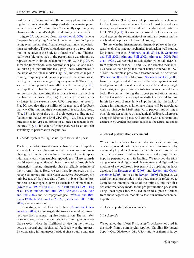
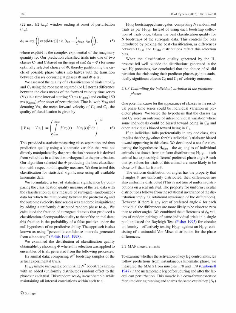
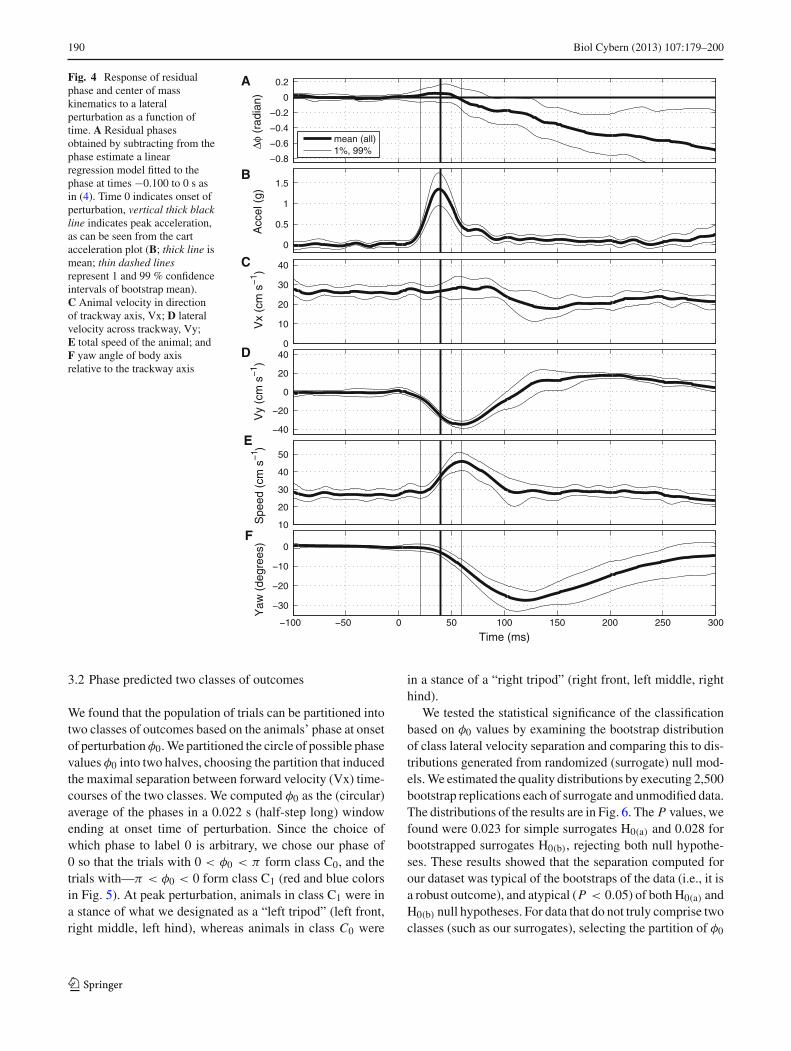
The overall outcomes of lateral perturbation are shown inFig. 4 with 1 and 99 % confidence intervals obtained froma bootstrap. Frequency decreased by 0.6 Hz as expressedby the negative slope of the Fig. 4A. Forward velocity (Vx)decreased from 26.1 ± 0.3 to 20.2 ± 0.8 cm s−1 found inthe mean shift of Fig. 4C. Lateral velocity (Vy) decreasedto −34.5 ± 0.9 cm s−1 followed by a return to zero andovershoot to 17.0 ± 0.3 cm s−1 before returning to zero(Fig. 4D). Ground speed showed a transient increase to45.5±0.9 cm s−1 from the initial speed of 27.3±0.4 cm s−1

(Fig. 4E). Yaw, the direction of the body axis with respect tothe cart, changed at its peak by 28.6◦ ± 0.7◦ (Fig. 4F).

Changes appeared at a delay from onset of perturbation.The earliest change manifests in lateral velocity (Fig. 4D)which became significant within less than 25 ms. This wasfollowed by ground speed and yaw angle at 40 ms (Fig. 4E, F).Forward velocity showed a change in trend at 70 ms. By 250ms, mean yaw angle was between −5◦ and 10◦, and by 300ms the confidence interval for lateral velocities included zero.

123

190 Biol Cybern (2013) 107:179–200

Fig. 4 Response of residualphase and center of masskinematics to a lateralperturbation as a function oftime. A Residual phasesobtained by subtracting from thephase estimate a linearregression model fitted to thephase at times −0.100 to 0 s asin (4). Time 0 indicates onset ofperturbation, vertical thick blackline indicates peak acceleration,as can be seen from the cartacceleration plot (B; thick line ismean; thin dashed linesrepresent 1 and 99 % confidenceintervals of bootstrap mean).C Animal velocity in directionof trackway axis, Vx; D lateralvelocity across trackway, Vy;E total speed of the animal; andF yaw angle of body axisrelative to the trackway axis

−0.8

−0.6

−0.4

−0.2

0

0.2A

Δφ (

radi

an)

mean (all)1%, 99%

0

0.5

1

1.5

Acc

el (

g)

B

0

10

20

30

40V

x (c

m s

−1 )

C

−40

−20

0

20

40

Vy

(cm

s−

1 )

D

10

20

30

40

50

Spe

ed (

cm s

−1 )E

−100 −50 0 50 100 150 200 250 300

−30

−20

−10

0

Yaw

(de

gree

s)

F

Time (ms)

3.2 Phase predicted two classes of outcomes

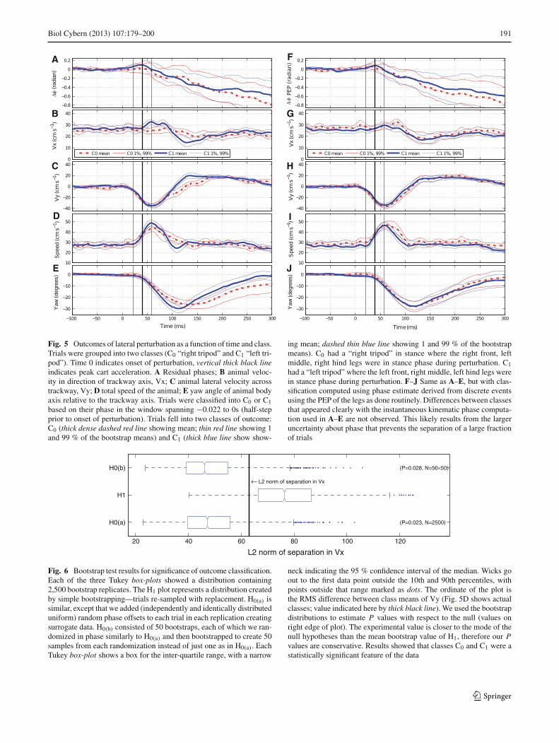
We found that the population of trials can be partitioned intotwo classes of outcomes based on the animals’ phase at onsetof perturbation φ0. We partitioned the circle of possible phasevalues φ0 into two halves, choosing the partition that inducedthe maximal separation between forward velocity (Vx) time-courses of the two classes. We computed φ0 as the (circular)average of the phases in a 0.022 s (half-step long) windowending at onset time of perturbation. Since the choice ofwhich phase to label 0 is arbitrary, we chose our phase of0 so that the trials with 0 < φ0 < π form class C0, and thetrials with—π < φ0 < 0 form class C1 (red and blue colorsin Fig. 5). At peak perturbation, animals in class C1 were ina stance of what we designated as a “left tripod” (left front,right middle, left hind), whereas animals in class C0 were

in a stance of a “right tripod” (right front, left middle, righthind).

We tested the statistical significance of the classificationbased on φ0 values by examining the bootstrap distributionof class lateral velocity separation and comparing this to dis-tributions generated from randomized (surrogate) null mod-els. We estimated the quality distributions by executing 2,500bootstrap replications each of surrogate and unmodified data.The distributions of the results are in Fig. 6. The P values, wefound were 0.023 for simple surrogates H0(a) and 0.028 forbootstrapped surrogates H0(b), rejecting both null hypothe-ses. These results showed that the separation computed forour dataset was typical of the bootstraps of the data (i.e., it isa robust outcome), and atypical (P < 0.05) of both H0(a) andH0(b) null hypotheses. For data that do not truly comprise twoclasses (such as our surrogates), selecting the partition of φ0

123

Biol Cybern (2013) 107:179–200 191

A F

B G

C H

D I

E J

Fig. 5 Outcomes of lateral perturbation as a function of time and class.Trials were grouped into two classes (C0 “right tripod” and C1 “left tri-pod”). Time 0 indicates onset of perturbation, vertical thick black lineindicates peak cart acceleration. A Residual phases; B animal veloc-ity in direction of trackway axis, Vx; C animal lateral velocity acrosstrackway, Vy; D total speed of the animal; E yaw angle of animal bodyaxis relative to the trackway axis. Trials were classified into C0 or C1based on their phase in the window spanning −0.022 to 0s (half-stepprior to onset of perturbation). Trials fell into two classes of outcome:C0 (thick dense dashed red line showing mean; thin red line showing 1and 99 % of the bootstrap means) and C1 (thick blue line show show-

ing mean; dashed thin blue line showing 1 and 99 % of the bootstrapmeans). C0 had a “right tripod” in stance where the right front, leftmiddle, right hind legs were in stance phase during perturbation. C1had a “left tripod” where the left front, right middle, left hind legs werein stance phase during perturbation. F–J Same as A–E, but with clas-sification computed using phase estimate derived from discrete eventsusing the PEP of the legs as done routinely. Differences between classesthat appeared clearly with the instantaneous kinematic phase computa-tion used in A–E are not observed. This likely results from the largeruncertainty about phase that prevents the separation of a large fractionof trials

20 40 60 80 100 120

H0(a)

H1

H0(b)

L2 norm of separation in Vx

← L2 norm of separation in Vx

(P=0.023, N=2500)

(P=0.028, N=50×50)

Fig. 6 Bootstrap test results for significance of outcome classification.Each of the three Tukey box-plots showed a distribution containing2,500 bootstrap replicates. The H1 plot represents a distribution createdby simple bootstrapping—trials re-sampled with replacement. H0(a) issimilar, except that we added (independently and identically distributeduniform) random phase offsets to each trial in each replication creatingsurrogate data. H0(b) consisted of 50 bootstraps, each of which we ran-domized in phase similarly to H0(a) and then bootstrapped to create 50samples from each randomization instead of just one as in H0(a). EachTukey box-plot shows a box for the inter-quartile range, with a narrow

neck indicating the 95 % confidence interval of the median. Wicks goout to the first data point outside the 10th and 90th percentiles, withpoints outside that range marked as dots. The ordinate of the plot isthe RMS difference between class means of Vy (Fig. 5D shows actualclasses; value indicated here by thick black line). We used the bootstrapdistributions to estimate P values with respect to the null (values onright edge of plot). The experimental value is closer to the mode of thenull hypotheses than the mean bootstrap value of H1, therefore our Pvalues are conservative. Results showed that classes C0 and C1 were astatistically significant feature of the data

123

192 Biol Cybern (2013) 107:179–200

values that induces the greatest class separation is more than95 % likely to induce less separation than we observed inour data and in a large majority of randomly selected resam-ples from our data. This indicates that the classification weextracted is a reliable feature of the data rather than an artifactof data analysis. We performed this same analysis using thephase estimate derived from the PEPs of the legs (Fig. 5F–J).In this case, the distribution obtained for class forward veloc-ity separation (Fig. 5G) under the H1 hypothesis was statis-tically indistinguishable from the surrogates H0(a) and H0(b)

(P > 0.1 in both cases). We attribute this loss of significanceto the lower temporal resolution afforded by a phase estimatederived from discrete events (i.e., a non-instantaneous phaseestimate).

The classes C0 and C1 were divided with 25 trials in C0

and to 16 trials in C1, giving a χ2 = 1.98 with P = 0.16. Thetrials thus fell into classes with probabilities indistinguish-able from random. The Rayleigh test applied to bootstrapsamples of the 32 trials which came from animals that ranmore than one trial gave Rayleigh test statistics with 10 and90 % quantiles of 0.09 and 1.87, respectively, and a mean of0.8, corresponding to P values all of which are larger than0.1, and thus robustly (for nearly all bootstraps) failed toreject the null hypothesis of uniformly distributed φ0 valuesper individual. We conclude that our classification was notproduced by individual variation in animal responses, or inother words that no individual experienced the perturbationin any class (i.e., “left tripod” or “right tripod”) more oftenthan expected at random.

3.3 Kinematic differences between the classes

Comparing the results in Figs. 4 and 5, the structure generat-ing outcome variability in Fig. 4 becomes evident. WhereasFig. 4C–F showed changes in variability around the mean atdifferent delays from onset of perturbation, the correspond-ing plots in Fig. 5B–E showed that each class has uniformwithin-class variability over time. Thus, the large changesin variability in Fig. 4 are accounted for by distributing out-comes into two classes. Furthermore, Fig. 5F–J contains thekinematic outcomes arising from the classification obtainedfrom the PEP phase estimate. The lack of statistical signifi-cance for this classification is manifest in the indistinguish-able kinematic outcomes of the two classes.

The C1 trials (left tripod down) showed initial statisticallysignificant, but small in magnitude increases in phase and for-ward speed from zero at approximately 0.045 s after onset ofperturbation (Fig. 5A, B; solid blue) relative to C0 trials. Wesuspected that this change might not be due to neural clockchanges and is instead due to direct mechanical effects ofbody yaw on the stance legs. As our phase estimate uses theswing tarsi in the body frame of reference, it is partially iso-lated from mechanical influence on the stance tarsi. However,

at the moment of lift-off, because stance tarsi are attachedto the ground, yaw might induce a systematic structure inthe velocities of tarsi which carries through into swing andcould appear as a change in phase. To inform our understand-ing of how much of the C1 class-specific phase increase isdue to this effect, we introduced a simulated pattern of unper-turbed tarsus positions into a body frame of reference derivedfrom experimental data, then clamped the stance legs to theworld frame at touchdown, and relaxed them back to theirunperturbed body frame position within 16 ms—the rate ofmechanical relaxation identified by Dudek and Full [2007].The goal of this simulation of “feed-forward” tarsus motionsattached to experimentally derived center of mass (COM) tra-jectories is to reproduce a plausible model for the motions ofthe tarsi of an animal which is activating its legs without anyfeedback modulation. These simulated animals exhibited aclass-specific phase change similar to that seen in the exper-imental data in the 0.045s region under discussion. If thatphase change is taken into account, the confidence intervalsfor C1 in Fig. 5A would include zero. We conclude that thesmall increase we observed is likely due to this mechanism.

C1 trials lateral velocity recovered and overshot faster(Fig. 5C, solid blue). They reached the peak overshoot value0.050 s before C0 trials (Fig. 5A, B, dashed red). Yaw ofC1trials fully recovered within less than 0.30 s (Fig. 5E,solid blue), whereas animals represented in C0 trials (Fig. 5E,dashed red) never recovered their original yaw angle withinthe period measured.

3.4 Residual phase change represents a frequency change

Starting with onset of perturbation (time = 0), animalsshowed no significant change in kinematic phase for 0.030s—nearly the duration of an entire step. After that time, fre-quency increased (see Fig. 4A mean), but this increase wasstatistically significant for less that 0.025 s in the first half ofthe perturbation, and only in the C1 class of trials (Fig. 5A,solid blue). Within the next 0.050 s, residual phase changedto follow a new trend-line, corresponding to a >5 % decreasein the frequency of animal tarsus cycling, decreasing from11.0 ± 0.2 Hz by 0.6 Hz.

We conclude that kinematic evidence for neural feedback,in the form of a persistent frequency change, appeared in therecovery of cockroaches from lateral perturbation. Frequencydecrease appeared at a delay, and the delay was not a functionof the animal’s posture (i.e., C0 vs. C1), although the actualchange in kinematics —differences in COM velocity—wasposture (class) dependent.

3.5 Muscle action potentials

We collected 37 trials from 7 male cockroaches with a mass2.32 ± 0.32 g. Animals ran at a speed of 0.362 ± 0.070

123

Biol Cybern (2013) 107:179–200 193

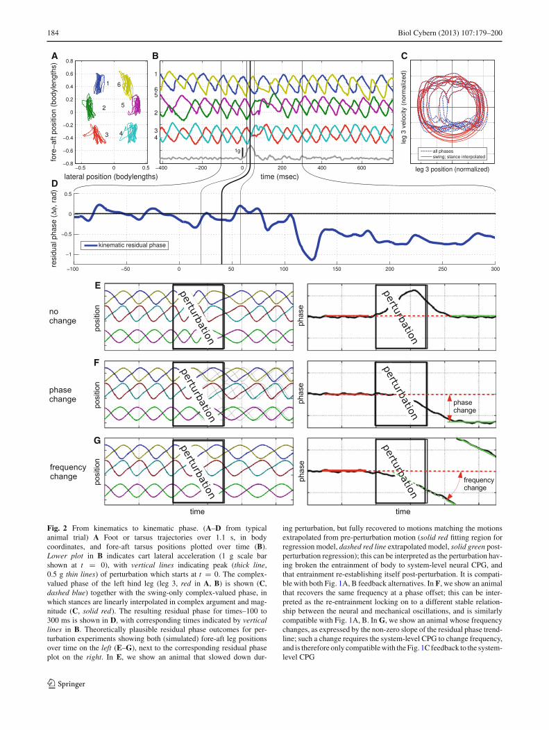
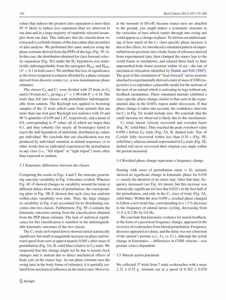
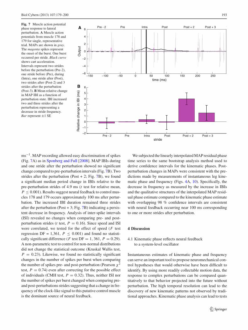
Fig. 7 Muscle action potentialphase response to lateralperturbation. A Muscle actionpotentials from muscle 178 and179 for single, representativetrial. MAPs are shown in gray.The magenta spikes representthe onset of the burst. One burstoccurred per stride. Black curveshows cart acceleration.Intervals represent two stridesbefore the perturbation (Pre-2),one stride before (Pre), during(Intra), one stride after (Post),two strides after (Post-2) and 3strides after the perturbation(Post-3). B Mean relative changein MAP IBI as a function ofperturbation state. IBI increasedtwo and three strides after theperturbation representing adecrease in stride frequency.Bar represent ±1 SE

25

Pre - 2 Pre Intra Post Post + 2 Post + 3−150 −100 −50 0 50 100 150 200 250

time (ms)−150 −100 −50 0 50 100 150 200 250

time (ms)

A

B

−150 −100 −50 0 50 100 150 200 250−6

−4

−2

0

2

4

6Pre - 2 Pre Intra Post Post + 2 Post + 3

Out

put

time (ms)

−2

−1

0

1

2

3

4

5

6

Rel

ativ

e ch

ange

in IB

I (m

s)

Pre - 2 Pre Intra Post Post + 2 Post + 3stride

ms−1. MAP recording allowed easy discrimination of spikes(Fig. 7A) as in Sponberg and Full [2008]. MAP IBIs duringand one stride after the perturbation showed no significantchange compared to pre-perturbation intervals (Fig. 7B). Twostrides after the perturbation (Post + 2; Fig. 7B), we founda significant median period change in IBIs relative to thepre-perturbation strides of 4.9 ms (t test for relative mean,P ≤ 0.001). Results suggest neural feedback to control mus-cles 178 and 179 occurs approximately 100 ms after pertur-bation. The increased IBI duration remained three stridesafter the perturbation (Post + 3; Fig. 7B) indicating a persis-tent decrease in frequency. Analysis of inter-spike intervals(ISI) revealed no changes when comparing pre- and post-perturbation strides (t test, P = 0.16). Since speed and ISIwere correlated, we tested for the effect of speed (F testregression DF = 1,361, P ≤ 0.001) and found no statisti-cally significant difference (F test DF = 1, 361, P = 0.29).A non-parametric test to control for non-normal distributionsdid not change the statistical outcome (Kruskal Wallis test,P = 0.23). Likewise, we found no statistically significantchanges in the number of spikes per burst when comparingthe number of spikes pre- and post-perturbation (Pearson χ2

test, P = 0.74) even after correcting for the possible effectof individuals (CMH test, P = 0.32). Thus, neither ISI northe number of spikes per burst changed when comparing pre-and post-perturbations strides suggesting that a change in fre-quency of the clock-like signal to this putative control muscleis the dominant source of neural feedback.

We subjected the linearly interpolated MAP residual phasetime series to the same bootstrap analysis method used toderive confidence intervals for the kinematic phases. Post-perturbation changes in MAPs were consistent with the pre-dictions made by measurements of instantaneous leg kine-matic phase and frequency (Figs. 4A, 10). Specifically, thedecrease in frequency as measured by the increase in IBIsand the qualitative structures of the interpolated MAP resid-ual phase estimate compared to the kinematic phase estimatewith overlapping 98 % confidence intervals are consistentwith neural feedback occurring near 100 ms correspondingto one or more strides after perturbation.

4 Discussion

4.1 Kinematic phase reflects neural feedbackto a system-level oscillator

Instantaneous estimates of kinematic phase and frequencycan serve an important tool to propose neuromechanical con-trol hypotheses that would otherwise have been difficult toidentify. By using more readily collectable motion data, theresponse to complex perturbations can be compared quan-titatively to that behavior projected into the future withoutperturbation. The high temporal resolution can lead to thediscovery of new kinematic patterns not observed by tradi-tional approaches. Kinematic phase analysis can lead to tests

123

194 Biol Cybern (2013) 107:179–200

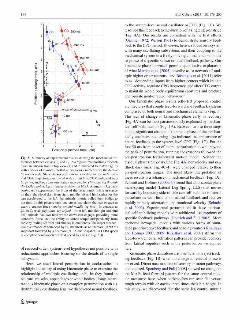
Fig. 8 Summary of experimental results showing the mechanical dif-ferences between classes C0 and C1. Average animal positions for eachclass are shown from a top view (X and Y indicated to match Fig. 3)with a series of symbols plotted at positions sampled from the data at50 ms intervals. Stance tarsus positions indicated by empty circles, ani-mal COM trajectories are traced with a solid line, COM indicated by alarge dot, and body axis orientation indicated by a line passing throughthe COM symbol. Cart impulse is shown in black. Animals in C0 trials(right; red) experienced the brunt of the perturbation while in stanceon the right tripod (i.e., front right, middle left and hind right). As thecart accelerated to the left, the animals’ inertia pulled their bodies tothe right. In this posture only one tarsus had claws that can engage toexert a counter-force (circles around middle leg foot). In contrast toC0, in C1 trials (left; blue; left tripod—front left, middle right and hindleft) animals had two tarsi whose claws can engage, providing morecorrective force, and the ability to correct torque independently fromforce by trading off front and hind leg lateral forces. The larger mechan-ical disturbance experienced by C0 manifests as an increase (at 90 mssnapshot) followed by a decrease (at 190 ms snapshot) in COM speed(a complete comparison of COM speed by class in Fig. 5D)

of reduced-order, system-level hypotheses not possible withreductionist approaches focusing on the details of a singlesubsystem.

Here, we used lateral perturbation in cockroaches tohighlight the utility of using kinematic phase to examine therelationship of multiple oscillating units, be they found inneurons, muscles, appendages or whole bodies. Using instan-taneous kinematic phase on a complex perturbation with sixrhythmically oscillating legs, we discovered neural feedback

to the system-level neural oscillator or CPG (Fig. 1C). Weresolved this feedback to the duration of a single step or stride(Fig. 4A). Our results are consistent with the first efforts(Grillner 1972; Wilson 1961) to demonstrate sensory feed-back to the CPG period. However, here we focus on a systemwith many oscillating subsystems and their coupling to themechanical system in a freely moving animal and not on theresponse of a specific sensor or local feedback pathway. Ourkinematic phase approach permits quantitative explorationof what Marder et al. [2005] describe as “a network of mul-tiple higher order neurons” and Büschges et al. [2011] referto as “descending inputs from higher centers which initiateCPG activity, regulate CPG frequency, and alter CPG outputto maintain whole body equilibrium (posture) and produceappropriate goal-directed behaviour.”

Our kinematic phase results reflected proposed controlarchitectures that couple feed-forward and feedback systemscomprised of both neural and mechanical elements (Fig. 1).The lack of change in kinematic phase early in recovery(Fig. 4A) can be most parsimoniously explained by mechan-ical self-stabilization (Fig. 1A). Between two to three stepslater, a significant change in kinematic phase of the mechan-ically unconstrained swing legs indicates the appearance ofneural feedback to the system-level CPG (Fig. 1C). For thefirst 50 ms from onset of lateral perturbation to well beyondthe peak of perturbation, running cockroaches followed thepre-perturbation feed-forward motion model. Neither theresidual phase (thick dark line, Fig. 4A) nor velocity and yaw(thick dark lines, Fig. 4C–F) were changed relative to theirpre-perturbation ranges. The most likely interpretation ofthese results is a reliance on mechanical feedback (Fig. 1A).Schmitt and Holmes (2000a, b) found that a horizontal planemass-spring model (Lateral Leg Spring, LLS) that movesforward by bouncing side-to-side can self-stabilize to lateralperturbations with little or no neural feedback and recoverrapidly in body orientation and rotational velocity (Schmittet al. 2002). Experimental perturbations fit these mechan-ical self-stabilizing models with additional assumptions ofspecific feedback pathways (Jindrich and Full 2002). Moreanchored hexapedal models with various forms of simu-lated proprioceptive feedback and heading control (Kukillayaand Holmes 2007, 2009; Kukillaya et al. 2009) affirm thatfeed-forward neural activation patterns can provide recoveryfrom lateral impulses such as the perturbation we appliedhere.

Kinematic phase data alone are insufficient to reject track-ing feedback (Fig. 1B) when no change in residual phase isobserved. Direct measurement of sensory or motor pathwaysare required. Sponberg and Full [2008] showed no change inthe MAPs feed-forward pattern for the same control mus-cle measured here, when cockroaches ran over flat versusrough terrain with obstacles three times their hip height. Inthis study, we discovered that the same leg control muscle

123

Biol Cybern (2013) 107:179–200 195

did not alter its feed-forward IBI until 100 ms after peakperturbation and 140 ms after perturbation onset that corre-sponds to one or more strides after the maximum perturbation(Fig. 7). Yet, our kinematic data show a nearly-completerecovery of lateral velocity (Fig. 4D) before the MAP inter-burst duration change (Fig. 7B) or the residual kinematicphase changes (Fig. 4A). Certainly, one cannot rule out thepossibility that another feature of the MAP pattern includesearlier feedback information, that the next muscle we mea-sure might demonstrate neural feedback, or that extraordi-narily rapid reflexes (Holtje and Hustert 2003) are coupled tomuscles with extremely rapid force development acting withlittle delay when played through a viscoelastic mechanicalsystem. However, for dynamic locomotion where bandwidthlimitations become important, the more the initial responseto perturbation data are explained by mechanical feedbackusing feed-forward signals, the more the burden of proofshifts to finding a neural, sensory or muscle activation pat-tern whose change demonstrably affects the dynamics of thewhole body in the observed time course of the perturbationand recovery (Holmes et al. 2006).

Kinematic phase data do support neural feedback to thesystem-level CPG following the perturbation. After a step,the mean residual phase established a new trend (thick darkline, Fig. 4A) with its slope corresponding to an averagedecrease in frequency by 0.6 Hz from the pre-perturbationvalues of 11.0±0.2 Hz. The frequency change correspondedto an outcome of the form shown in Fig. 2G, and rejectedboth purely mechanical feedback (Fig. 1A) and tracking feed-back (Fig. 1B) in favor of feedback to the system-level CPG(Fig. 1C). The increase in MAP IBIs of a key leg controlmuscle (Fig. 7B) paralleled the decrease in residual phase(Fig. 4A) and therefore stride frequency both in magnitudeand stride-by-stride timing.

Further supporting evidence for system-level CPG feed-back comes from the same species for six of the 150steps analyzed for rough terrain running (Sponberg and Full2008). In these few steps, the animal failed to make groundcontact during its normal gait cycle, resulting in very largeperturbations that presumably drove the animal out of its pas-sive basin of stability. Despite the lack of stance initiation,the rhythmic activation of control muscles persisted for onestep, suggesting a continuation of the feed-forward, CPG sig-nal (Fig. 7b, c in Sponberg and Full 2008). Examination ofthe next stride showed that neural feedback acted to delaystance initiation. During these very large perturbations, thedorsal/ventral femoral extensors did not use sensory infor-mation to adjust this muscle within a stride, but acted to shiftthe phase of the system-level CPG’s clock-like signal in thesubsequent stride.

Most recently, in middle leg muscles homologous to thecontrol muscle measured in this study, Sponberg et al. (2011a,b) manipulated a freely running animal by reading each neu-

rally produced MAP to trigger additional artificially pro-duced voltage spikes mimicking a modified neural feedbackwhile capturing limb and body dynamics through high-speedvideography and a microaccelerometer backpack. Despitechanges in timing of the stride where stimulation was intro-duced, the next stride acted to re-synchronize the alternatingtripod such that future strides were indistinguishable frombefore the added feedback-like signal. This suggested thatthere was no change to the system-level CPG timing of thealternating tripod gait. Their results are consistent with asystem-level CPG acting to establish steady-state runningdynamics and neural feedback impinging on these activa-tion patterns below the level where system-level CPG timingoccurs.

Our kinematic phase results and MAP recordings duringa lateral perturbation of a rapid running animal add to thedeveloping picture of the control of locomotion based onanimals in which the dynamics of locomotion play a lesserrole (Büschges et al. 2011; Büschges 2005). Büschges et al.[2011] argue that motor signaling in stick insects is generatedby neural CPGs (each of which typically generates signalingto a single antagonistic set of muscles) located in a segmentproximal to the muscles they control, and whose functionis modulated by descending signals. Our results are consis-tent with this architecture, but we suggest three nested controlloops acting at substantially separated time constants (Fig. 1).The outermost, slowest loop involves modulation of theCPGs by descending higher brain centers or high order neuralnetworks. The mid-range loop, reacting at time constants ofsingle strides, interlocks the neural CPGs into a single, some-what higher system-level CPG. The inner, fastest loop, whichhandles within-stride stabilization in time constants of a frac-tional step, is most often implemented mechanically, but doesnot preclude the possibility of an extremely fast “supportreflex” such as been proposed in locust (Holtje and Hustert2003).

Support for a nested, hierarchical neuromechanical con-trol architecture continues to emerge (Revzen et al. 2008).Fuchs et al. [2011] state for the neural system in cock-roaches, “In the absence of sensory feedback, we observeda coordination pattern with consistent phase relationshipthat shares similarities with a double-tripod gait, suggestingcentral, feed-forward control.” Kukillaya et al. [2009] char-acterizing the mechanical system conclude that, “the feedfor-ward CPG-driven system is marginally stable, with a weaklystable mode and a neutral mode, making it act as a low-pass filter that yields fairly easily correctable and steerabledynamics.”

We hypothesize that the passive mechanical system is suf-ficiently stable to recover from small perturbations, but notso stable as to obviate the contribution of neural feedback atseveral levels to recover from large perturbations as deliveredin the present experiments.

123

196 Biol Cybern (2013) 107:179–200

4.2 Classes of kinematic outcome—effect of leg numberand position on lateral stability

Velocity of COM evolved in two different ways dependingon pre-perturbation phase leg pose (Fig. 5B, C). The twoclasses represented statistically significant differences in out-come (Fig. 6), pointing to the power of kinematic phase asa succinct representation of animal state, and thus a pre-dictor of future outcomes. The fact that a phase estimatederived from discrete (PEP) events did not yield a statisti-cally significant kinematic classification in our experiment(Fig. 5G, H) indicates that the increased temporal resolutionafforded by instantaneous estimates of kinematic phase pro-vides a more accurate description of an animal’s state. Froma dynamical systems perspective, the success of phase at pre-dicting future outcomes is not surprising—any stable nonlin-ear oscillator (such as running animals) can be modeled asa periodic function of phase using Floquet theory (Floquet1883; Guckenheimer and Holmes 1983), a fact that may makekinematic phase-based methods invaluable to future biome-chanical studies.

We hypothesize that the differences in COM velocity andyaw rate between the two outcome classes (Fig. 5B–E) are theconsequence of differences in passive mechanical stabilitywith respect to the perturbation. As the cart accelerated tothe animals’ left, they experienced a force to their right withrespect to the cart frame of reference. In C1 trials, animalswere mostly in a left tripod stance with the front left, middleright, and hind left legs on the cart during peak perturbation(Fig. 8, blue). In C0 trials, animals were in right stance withthe front right, middle left and hind right on the cart duringpeak perturbation (Fig. 8, red). As the animal began to bepulled laterally, the claws of the two feet on its left side couldengage the substrate to exert considerable lateral force. ForC0 trials, only the middle leg claws were available on its leftside. The animal also experienced a torque when the clawson the middle leg engaged, as the middle leg was typically infront of the center of mass. For C1 trials, the two sets of clawswere located anterior and posterior to the COM. This couldallow for a larger lateral force and for the forces to be paired,thus minimizing the torque and facilitating recovery whilebetter preserving orientation and heading. In this manner,animals in the C1 trials could rely on the mechanical feedbackpathway (Fig. 1A) to compensate for a greater part of theperturbation than animals in the C0 trials, and experiencedfaster recovery to their final lateral velocity (Vy, Fig. 5C,blue) and more rapid recovery of yaw angle (Fig. 5E, blue).

Kinematic phase allowed us to reduce posture to a univari-ate time series, so we were able to attribute the difference inperturbation recovery of class C0 versus C1 trials to a spe-cific animal pose (Fig. 8). While it is commonly assumedthat hexapedal designs are the most stable of legged run-ners because of their ability to maintain a static stability

margin throughout the gait cycle or dynamically move theCOM into the next tripod of support (Ting et al. 1994), ourresults from lateral perturbations expose a limitation of thehexapods’ alternating tripod gait. As illustrated in Fig. 8, theC0 class (red) is constrained in its ability to exert restora-tive forces and torques, because only one leg is available onthat side of the animal’s body. We hypothesize that sprawledmorphologies with at least two legs in stance on each sideof the body will have a significant advantage in recoveringfrom lateral perturbations, and thus may be a useful designtarget for legged robots. Perhaps animals and robots witheight or more legs would be more robust to lateral pertur-bations. Initial performance evaluations of a new 8-leggedrobot (OctoRoaACH) are consistent with these predictions(Pullin et al. 2012).

4.3 Kinematic phase as a tool for neuromechanical andneuroethological studies

We compared the residual from our instantaneous kine-matic phase to the residual from phase computed from thetiming of posterior extreme positions (PEP) of a selectedleg, as commonly used in the biomechanics literature(Cruse et al. 1998; Bender et al. 2010; Maes et al. 2008).Depending on which leg we chose, we observed qualitativelydifferent residual phase outcomes: from no change whenusing the left front leg (Fig. 9C), to a frequency increasewhen using the right middle leg (Fig. 9D). Averaging (circu-lar average, Fisher 1993) the PEP phase estimates from all sixlegs (Fig. 9B) gave a residual phase that most closely resem-bled our own (Fig. 9A), suggesting that the present methodprovides a reliable representation of the global phase. Weassert that our approach—estimating a phase from the instan-taneous state at every sample—resolves true phase (in thedynamical systems sense) much more accurately than meth-ods based on events such as PEP, foot touchdown, EMG IBIs,and other similar events. In those cases where the investigatorhypothesizes there to be multiple interacting clocks, such asindependent clocks for separate legs, each clock’s kinematicphase estimate can be generated from the multiple kinematicmeasurements that it drives (Revzen et al. 2008), and the cou-pling between these clocks can then be explored (Kralemannet al. 2007).

Though the phase estimates we derive from PEP eventsand from instantaneous kinematic data are qualitatively simi-lar (compare Fig. 9A, B), the high temporal resolution intrin-sic to instantaneous estimates of phase provide greater insightinto the mechanical state of the animal. Specifically, ourinstantaneous estimate of kinematic phase enabled the iden-tification of a significant difference in kinematic response toa large lateral perturbation based on the mechanical config-uration of the animal immediately prior to onset of the per-turbation. This result was obscured when using less resolved

123

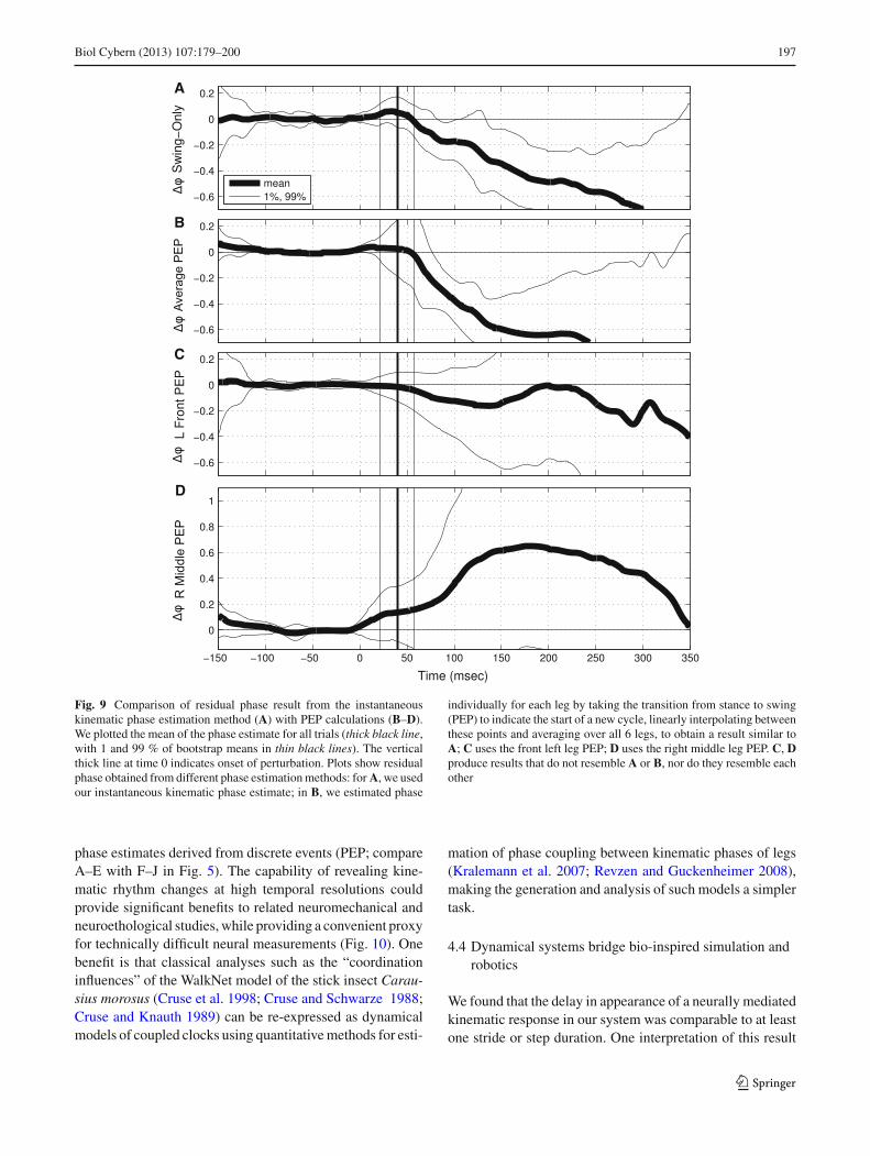
Biol Cybern (2013) 107:179–200 197

A

B

C

D

Fig. 9 Comparison of residual phase result from the instantaneouskinematic phase estimation method (A) with PEP calculations (B–D).We plotted the mean of the phase estimate for all trials (thick black line,with 1 and 99 % of bootstrap means in thin black lines). The verticalthick line at time 0 indicates onset of perturbation. Plots show residualphase obtained from different phase estimation methods: for A, we usedour instantaneous kinematic phase estimate; in B, we estimated phase

individually for each leg by taking the transition from stance to swing(PEP) to indicate the start of a new cycle, linearly interpolating betweenthese points and averaging over all 6 legs, to obtain a result similar toA; C uses the front left leg PEP; D uses the right middle leg PEP. C, Dproduce results that do not resemble A or B, nor do they resemble eachother

phase estimates derived from discrete events (PEP; compareA–E with F–J in Fig. 5). The capability of revealing kine-matic rhythm changes at high temporal resolutions couldprovide significant benefits to related neuromechanical andneuroethological studies, while providing a convenient proxyfor technically difficult neural measurements (Fig. 10). Onebenefit is that classical analyses such as the “coordinationinfluences” of the WalkNet model of the stick insect Carau-sius morosus (Cruse et al. 1998; Cruse and Schwarze 1988;Cruse and Knauth 1989) can be re-expressed as dynamicalmodels of coupled clocks using quantitative methods for esti-

mation of phase coupling between kinematic phases of legs(Kralemann et al. 2007; Revzen and Guckenheimer 2008),making the generation and analysis of such models a simplertask.

4.4 Dynamical systems bridge bio-inspired simulation androbotics

We found that the delay in appearance of a neurally mediatedkinematic response in our system was comparable to at leastone stride or step duration. One interpretation of this result

123

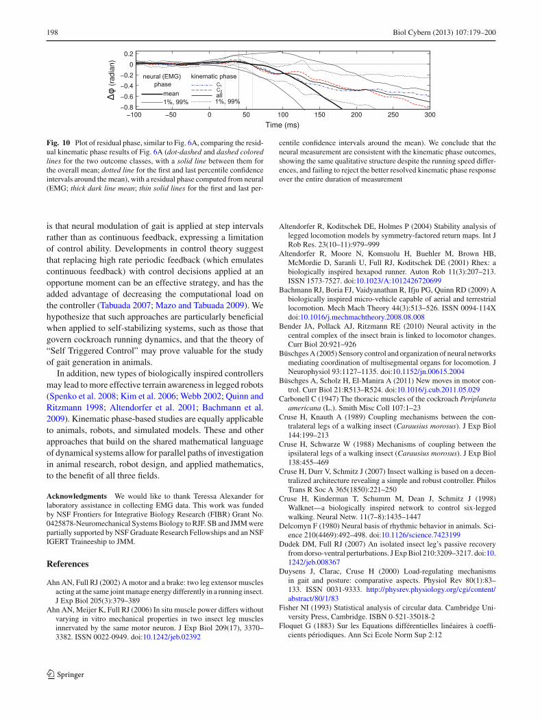
198 Biol Cybern (2013) 107:179–200

Fig. 10 Plot of residual phase, similar to Fig. 6A, comparing the resid-ual kinematic phase results of Fig. 6A (dot-dashed and dashed coloredlines for the two outcome classes, with a solid line between them forthe overall mean; dotted line for the first and last percentile confidenceintervals around the mean), with a residual phase computed from neural(EMG; thick dark line mean; thin solid lines for the first and last per-

centile confidence intervals around the mean). We conclude that theneural measurement are consistent with the kinematic phase outcomes,showing the same qualitative structure despite the running speed differ-ences, and failing to reject the better resolved kinematic phase responseover the entire duration of measurement

is that neural modulation of gait is applied at step intervalsrather than as continuous feedback, expressing a limitationof control ability. Developments in control theory suggestthat replacing high rate periodic feedback (which emulatescontinuous feedback) with control decisions applied at anopportune moment can be an effective strategy, and has theadded advantage of decreasing the computational load onthe controller (Tabuada 2007; Mazo and Tabuada 2009). Wehypothesize that such approaches are particularly beneficialwhen applied to self-stabilizing systems, such as those thatgovern cockroach running dynamics, and that the theory of“Self Triggered Control” may prove valuable for the studyof gait generation in animals.

In addition, new types of biologically inspired controllersmay lead to more effective terrain awareness in legged robots(Spenko et al. 2008; Kim et al. 2006; Webb 2002; Quinn andRitzmann 1998; Altendorfer et al. 2001; Bachmann et al.2009). Kinematic phase-based studies are equally applicableto animals, robots, and simulated models. These and otherapproaches that build on the shared mathematical languageof dynamical systems allow for parallel paths of investigationin animal research, robot design, and applied mathematics,to the benefit of all three fields.

Acknowledgments We would like to thank Teressa Alexander forlaboratory assistance in collecting EMG data. This work was fundedby NSF Frontiers for Integrative Biology Research (FIBR) Grant No.0425878-Neuromechanical Systems Biology to RJF. SB and JMM werepartially supported by NSF Graduate Research Fellowships and an NSFIGERT Traineeship to JMM.

References

Ahn AN, Full RJ (2002) A motor and a brake: two leg extensor musclesacting at the same joint manage energy differently in a running insect.J Exp Biol 205(3):379–389

Ahn AN, Meijer K, Full RJ (2006) In situ muscle power differs withoutvarying in vitro mechanical properties in two insect leg musclesinnervated by the same motor neuron. J Exp Biol 209(17), 3370–3382. ISSN 0022-0949. doi:10.1242/jeb.02392

Altendorfer R, Koditschek DE, Holmes P (2004) Stability analysis oflegged locomotion models by symmetry-factored return maps. Int JRob Res. 23(10–11):979–999

Altendorfer R, Moore N, Komsuolu H, Buehler M, Brown HB,McMordie D, Saranli U, Full RJ, Koditschek DE (2001) Rhex: abiologically inspired hexapod runner. Auton Rob 11(3):207–213.ISSN 1573-7527. doi:10.1023/A:1012426720699

Bachmann RJ, Boria FJ, Vaidyanathan R, Ifju PG, Quinn RD (2009) Abiologically inspired micro-vehicle capable of aerial and terrestriallocomotion. Mech Mach Theory 44(3):513–526. ISSN 0094-114Xdoi:10.1016/j.mechmachtheory.2008.08.008

Bender JA, Pollack AJ, Ritzmann RE (2010) Neural activity in thecentral complex of the insect brain is linked to locomotor changes.Curr Biol 20:921–926

Büschges A (2005) Sensory control and organization of neural networksmediating coordination of multisegmental organs for locomotion. JNeurophysiol 93:1127–1135. doi:10.1152/jn.00615.2004

Büschges A, Scholz H, El-Manira A (2011) New moves in motor con-trol. Curr Biol 21:R513–R524. doi:10.1016/j.cub.2011.05.029

Carbonell C (1947) The thoracic muscles of the cockroach Periplanetaamericana (L.). Smith Misc Coll 107:1–23

Cruse H, Knauth A (1989) Coupling mechanisms between the con-tralateral legs of a walking insect (Carausius morosus). J Exp Biol144:199–213

Cruse H, Schwarze W (1988) Mechanisms of coupling between theipsilateral legs of a walking insect (Carausius morosus). J Exp Biol138:455–469

Cruse H, Durr V, Schmitz J (2007) Insect walking is based on a decen-tralized architecture revealing a simple and robust controller. PhilosTrans R Soc A 365(1850):221–250

Cruse H, Kinderman T, Schumm M, Dean J, Schmitz J (1998)Walknet—a biologically inspired network to control six-leggedwalking. Neural Netw. 11(7–8):1435–1447

Delcomyn F (1980) Neural basis of rhythmic behavior in animals. Sci-ence 210(4469):492–498. doi:10.1126/science.7423199

Dudek DM, Full RJ (2007) An isolated insect leg’s passive recoveryfrom dorso-ventral perturbations. J Exp Biol 210:3209–3217. doi:10.1242/jeb.008367

Duysens J, Clarac, Cruse H (2000) Load-regulating mechanismsin gait and posture: comparative aspects. Physiol Rev 80(1):83–133. ISSN 0031-9333. http://physrev.physiology.org/cgi/content/abstract/80/1/83

Fisher NI (1993) Statistical analysis of circular data. Cambridge Uni-versity Press, Cambridge. ISBN 0-521-35018-2

Floquet G (1883) Sur les Equations différentielles linéaires à coeffi-cients périodiques. Ann Sci Ecole Norm Sup 2:12

123

Biol Cybern (2013) 107:179–200 199

Fuchs E, Holmes P, Kiemel T, Ayali A (2011) Intersegmental coordina-tion of cockroach locomotion: adaptive control of centrally coupledpattern generator circuits. Front Neural Circuits 4. doi:10.3389/fncir.2010.00125

Fuchs E, Holmes P, David I, Ayali A (2012) Proprioceptive feedbackreinforces centrally generated stepping patterns in the cockroach. JExp Biol 215:1884–1891. doi:10.1242/jeb.067488

Full RJ, Tu MS (1990) Mechanics of 6-legged runners. J Exp Biol148:129–146. ISSN 0022-0949

Full RJ, Blickhan R, Ting LH (1991) Leg design in hexapedal runners.J Exp Biol 158:369–390. ISSN 0022-0949

Full RJ, Stokes DR, Ahn A, Josephson RK (1998) Energy absorp-tion during running by leg muscles in a cockroach. J Exp Biol 201:997–1012

Full RJ, Koditschek DE (1999) Templates and anchors: neuromechan-ical hypotheses of legged locomotion on land. J Exp Biol 202:3325–3332

Ghigliazza RM, Altendorfer R, Holmes P, Koditschek DE (2005) Asimply stabilized running model. SIAM Rev 47(3):519–549

Grillner S (1972) The role of muscle stiffness in meeting the changingpostural and locomotor requirements for force development by theankle extensors. Acta Physiol Scand 86:92–108

Grillner S (1985) Neurobiological bases of rhythmic motor acts in ver-tebrates. Science 228:143–149

Grillner S, Wallén P (2002) Cellular bases of a vertebrate locomotorsystem—steering, intersegmental and segmental co-ordination andsensory control. Brain Res Rev 40(1–3):92–106

Guckenheimer J, Holmes P (1983) Nonlinear oscillations, dynamicalsystems, and bifurcations of vector fields. Springer, Berlin

Holmes P, Full RJ, Koditschek D, Guckenheimer J (2006) Dynamicsof legged locomotion: models, analyses, and challenges. SIAM Rev48(2):207–304

Holtje M, Hustert R (2003) Rapid mechano-sensory pathways codeleg impact and elicit very rapid reflexes in insects. J Exp Biol206(16):2715–2724. ISSN 0022-0949. doi:10.1242/jeb.00492

Ijspeert AJ (2008) Central pattern generators for locomotion control inanimals and robots: a review. Neural Netw. 21(4):642–653. ISSN0893-6080. doi:10.1016/j.neunet.2008.03.014

Jaric S, Latash ML (2000) The equilibrium-point hypothesis is stilldoing fine. Hum Mov Sci 19(6):933–938

Jindrich DL, Full RJ (1999) Many-legged maneuverability: dynamicsof turning in hexapods. J Exp Biol 202(12):1603–1623

Jindrich DL, Full RJ (2002) Dynamic stabilization of rapid hexapedallocomotion. J Exp Biol 205(18):2803–2823. ISSN 0022-0949

Kalman RE (1960) A new approach to linear filtering and predictionproblems. J Basic Eng 82:35–45

Kim S, Clark JE, Cutkosky MR (2006) iSprawl: design and tuningfor high-speed autonomous open-loop running. Int J Robot Res25(9):903–912. ISSN 0278-3649. doi:10.1177/0278364906069150

Klavins E, Komsuoglu H, Full RJ, Koditschek DE (2002) The roleof reflexes versus central pattern generators in dynamical leggedlocomotion. In: Ayers J, Davis J, Rudolph A (eds) Neurotechnologyfor biomimetic robots. MIT Press, Cambridge, pp 351–382

Kralemann B, Cimponerlu L, Rosenblum M, Pikovsky A, Mrowka R(2007) Uncovering interaction of coupled oscillators from data. PhysRev E 76(5):055201. ISSN: 1539-3655. doi:10.1103/PhysRevE.76.055201

Kram R, Wong B, Full RJ (1997) Three-dimensional kinematicsand limb kinetic energy of running cockroaches. J Exp Biol200(13):1919–1929. ISSN 0022-0949

Kubow TM, Full RJ (1999) The role of the mechanical system in control:a hypothesis of self-stabilization in hexapedal runners. Phil Trans RSoc B 354(1385):849–861. ISSN 0962-8436

Kukillaya RP, Holmes PJ (2007) A hexapedal jointed-leg model forinsect locomotion in the horizontal plane. Biol Cybern 97(5–6):379–395. ISSN 0340-1200. doi:10.1007/s00422-007-0180-2

Kukillaya RP, Holmes P (2009) A model for insect locomotion in thehorizontal plane: feedforward activation of fast muscles, stability,and robustness. J Theor Biol 261(2):210–226. doi:10.1016/j.jtbi.2009.07.036

Kukillaya R, Proctor J, Holmes P (2009) Neuromechanical modelsfor insect locomotion: stability, maneuverability, and proprioceptivefeedback. Chaos 19(2). ISSN 1054-1500. doi:10.1063/1.3141306

MacKay-Lyons M (2002) Central pattern generation of locomotion: areview of the evidence. Phys Ther 82(1):69–83. ISSN 0031-9023.http://www.ptjournal.org/cgi/content/abstract/82/1/69

Maes LD, Herbin M, Hackert R, Bels VL, Abourachid A (2008) Steadylocomotion in dogs: temporal and associated spatial coordinationpatterns and the effect of speed. J Exp Biol 211:138–149. doi:10.1242/jeb.008243

Marder E, Bucher D, Schulz D, Taylor A (2005) Invertebrate centralpattern generator moves along. Curr Biol 15:685–699

Mazo M, Tabuada P (2009) Input-to-state stability of self-triggered con-trol systems. In: Conference on decision and control, 48th IEEE,pp 928–933

Noah JA, Quimby L, Frazier SF, Zill SN (2004) Walking on a pegleg: extensor muscle activities and sensory feedback after distal legdenervation in cockroaches. J Comp Physiol A 190:217–231. ISSN0340-7594. doi:10.1007/s00359-003-0488-x

Pearson KG (1993) Common principles of motor control in vertebratesand invertebrates. Ann Rev Neurosci 16:265–297

Pearson KG (1995) Proprioceptive regulation of locomotion. Curr OpinNeurobiol 5:786–791

Pearson KG (2004) Generating the walking gait: role of sensory feed-back. Prog Brain Res 143:123–129

Pearson KG, Iles JF (1971) Innervation of coxal depressor muscles incockroach, Periplaneta americana. J Exp Biol 54(1):215–232

Pearson KG, Collins DF (1993) Reversal of the influence of group Ibafferents from plantaris on activity in medial gastrocnemius-muscleduring locomotor-activity. J Neurophysiol 70(3):1009–1017. ISSN0022-3077

Politis DN (1995) A primer on bootstrap methods in statistics. Tech-nical report 95-19. Purdue University. http://www.stat.purdue.edu/research/technical_reports/pdfs/1995/tr95-19.pdf

Politis DN (1998) Computer-intensive methods in statistical analysis.IEEE Signal Proc Mag 15(1):39–55. ISSN 1053-5888. doi:10.1109/79.647042

Prochazka A, Gillard D, Bennett DJ (1997a) Implications of positivefeedback in the control of movement. J Neurophysiol 77(6):3237–3251. ISSN 0022-3077

Prochazka A, Gillard, D, Bennett DJ (1997b) Positive force feedbackcontrol of muscles. J Neurophysiol 77(6):3226–3236. ISSN 0022-3077

Proctor J, Holmes PJ (2008) Steering by transient destabilization inpiecewise-holonomic models of legged locomotion. Regul ChaoticDyn 13(4):267–282. doi:10.1134/S1560354708040047

Proctor J, Holmes PJ (2010) Reflexes and preflexes: on the role ofsensory feedback on rhythmic patterns in insect locomotion. BiolCybern 102:513–531. doi:10.1007/s00422-010-0383-9

Proctor J, Kukillaya RP, Holmes P (2010) A phase-reduced neuro-mechanical model for insect locomotion: feed-forward stability andproprioceptive feedback. Phil Trans R Soc A 368:5087–5104

Pullin AO, Kohut NJ, Zarrouk D, Fearing RS (2012) Dynamic turn-ing of 13 cm robot comparing tail and differential drive. In: IEEEinternational conference on robotics and automation, May

Quinn RD, Ritzmann RE (1998) Construction of a hexapod robotwith cockroach kinematics benefits both robotics and biology.Connect Sci 10(3–4):239–254. ISSN 0954-0091. doi:10.1080/095400998116422

Rauch HE, Tung F, Striebel CT (1965) Maximum likelihood estimatesof linear dynamic systems. AIAA J 3(8):1445–1450. ISSN 0001-1452

123

200 Biol Cybern (2013) 107:179–200

Revzen S (2009) Neuromechanical control architectures of arthropodlocomotion. PhD Thesis. University of California, Berkeley

Revzen S, Guckenheimer JM (2008) Estimating the phase of syn-chronized oscillators. Phys Rev E 78(5):051907. ISSN 1539-3755.doi:10.1103/PhysRevE.78.051907

Revzen S, Koditschek DE, Full RJ (2008) Towards testable neuro-mechanical control architectures for running. In: Sternad D (ed)Progress in motor control—a multidisciplinary perspective, pp 25–56. Springer, New York doi:10.1007/978-0-387-77064-2-3

Ridgel AL, Ritzmann RE (2005) Effects of neck and circumoesophagealconnective lesions on posture and locomotion in the cockroach. JComp Physiol A 191(6):559–573

Ridgel A, Frazier F, Zill SN (2001) Dynamic responses of tibial cam-paniform sensilla studied by substrate displacement in freely mov-ing cockroaches. J Comp Physiol A 187(5):405–420. doi:10.1007/s003590100213

Ritzmann RE, Büschges A (2007) Adaptive motor behavior in insects.Curr Opin Neurobiol 17(6):629–636. ISSN 0959-4388. doi:10.1016/j.conb.2008.01.001

Schilling M, Cruse H, Arena P (2007) Hexapod walking: an expan-sion to walknet dealing with leg amputations and force oscilla-tions. Biol Cybern 96(3):323–340. ISSN 0340-1200. doi:10.1007/s00422-006-0117-1

Schmitt J, Holmes P (2000a) Mechanical models for insect locomotion:dynamics and stability in the horizontal plane I. Theory. Biol Cybern83(6):501–515

Schmitt J, Holmes P (2000b) Mechanical models for insect locomotion:dynamics and stability in the horizontal plane II. Application. BiolCybern 83(6):517–527

Schmitt J, Holmes P (2001) Mechanical models for insect locomotion:stability and parameter studies. Physica D 156(1–2):139–168

Schmitt J, Holmes P (2003) Mechanical models for insect locomotion:active muscles and energy losses. Biol Cybern 89(1): 43–55. ISSN0340-1200. doi:10.1007/s00422-003-0404-z

Schmitt J, Garcia M, Razo RC, Holmes P, Full RJ (2002) Dynamicsand stability of legged locomotion in the horizontal plane: a test caseusing insects. Biol Cybern 86(5):343–353

Seyfarth A, Geyer H, Herr H (2003) Swing-leg retraction: a simplecontrol model for stable running. J Exp Biol 206(15):2547–2555

Spagna JC, Goldman DI, Lin P-C, Koditschek DE, Full RJ (2007) Dis-tributed mechanical feedback in arthropods and robots simplifiescontrol of rapid running on challenging terrain. Bioinspir Biomim2(1): 9–18. ISSN 1748-3182. doi:10.1088/1748-3182/2/1/002

Spenko MJ, Haynes GC, Saunders JA, Cutkosky MR, Rizzi AA, FullRJ, Koditschek DE (2008) Biologically inspired climbing with ahexapedal robot. J Field Robot 25(4–5):223–242. ISSN 1556-4959.doi:10.1002/rob.20238

Spence AJ, Revzen S, Seipel J, Mullens C, Full RJ (2010) Insects run-ning on elastic surfaces. J Exp Biol 213:1907–1920. ISSN 0022-0949. doi:10.1242/jeb.042515

Sponberg S, Full RJ (2008) Neuromechanical response of musculo-skeletal structures in cockroaches during rapid running on roughterrain. J Exp Biol 211(3):433–446. ISSN 0022-0949. doi:10.1242/jeb.012385

Sponberg S, Libby T, Mullens C, Full RJ (2011a) Shifts in a singlemuscle’s control potential of body dynamics. Phil Trans R Soc B366:1606–1620. doi:10.1098/rstb.2010.0368

Sponberg S, Spence A, Mullens C, Full RJ (2011b) A single muscle’smultifunctional control potential of body dynamics for postural con-trol and running. Philos Trans R Soc B 366:1592–1605. doi:10.1098/rstb.2010.0367

Tabuada P (2007) Event-triggered real-time scheduling of stabilizingcontrol tasks. IEEE Trans Autom Control 52(9):1680–1685. ISSN0018-9286. doi:10.1109/TAC.2007.904277

Ting LH, Blickhan R, Full RJ (1994) Dynamic and static stability inhexapedal runners. J Exp Biol 197:251–269. ISSN 0022-0949

Watson JT, Ritzmann RE (1998a) Leg kinematics and muscle activityduring treadmill running in the cockroach, Blaberus discoidalis: I.Slow running. J Comp Physiol A 182(1):11–22. ISSN 0340-7594.doi:10.1007/s003590050153

Watson JT, Ritzmann RE (1998b) Leg kinematics and muscle activityduring treadmill running in the cockroach, Blaberus discoidalis: II.Fast running. J Comp Physiol A 182(1):23–33. ISSN 0340–7594.doi:10.1007/s003590050154

Watson JT, Ritzmann RE, Pollack AJ (2002a) Control of climbingbehavior in the cockroach, Blaberus discoidalis. II. Motor activitiesassociated with joint movement. J Comp Physiol A 188(1):55–69.ISSN 0340-7594. doi:10.1007/s00359-002-0278-x

Watson JT, Ritzmann RE, Zill SN, Pollack AJ (2002b) Control of obsta-cle climbing in the cockroach, Blaberus discoidalis. I. Kinematics.J Comp Physiol A 188(1):39–53. ISSN 0340-7594. doi:10.1007/s00359-002-0277-y

Webb B (2002) Robots in invertebrate neuroscience. Nature417(6886):359–363. ISSN 0028-0836

Wilson DM (1961) The central nervous control of flight in a locust. JExp Biol 38:471–490

Zehr EP, Stein RB (1999) What functions do reflexes serve duringhuman locomotion? Prog Neurobiol 58(2):185–205. ISSN 0301–0082

Zill SN, Moran DT, Varela, FG (1981) The exoskeleton and insect pro-prioception. 2. Reflex effects of tibial campaniform sensilla in theamerican cockroach, Periplaneta americana. J Exp Biol 94:43–55.ISSN 0022-0949

Zill SN, Schmitz J, Büschges A (2004) Load sensing and control ofposture and locomotion. Arthropod Struct Dev 33(3):273–286. ISSN1467-8039. doi:10.1016/j.asd.2004.05.005

Zill SN Keller BR, Duke ER (2009) Sensory signals of unloading in oneleg follow stance onset in another leg: transfer of load and emergentcoordination in cockroach walking. J Neurophysiol 101(5):2297–2304. ISSN 0022-3077. doi:10.1152/jn.00056.2009

123