Insertion DevicesLecture 2

Wigglers and Undulators

Jim ClarkeASTeC

Daresbury Laboratory

2

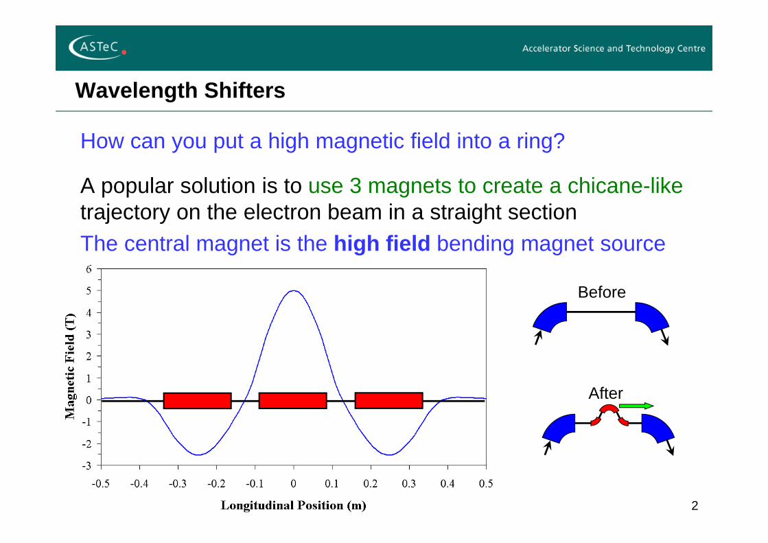
Wavelength Shifters

How can you put a high magnetic field into a ring?

A popular solution is to use 3 magnets to create a chicane-liketrajectory on the electron beam in a straight sectionThe central magnet is the high field bending magnet source

Before

After

3

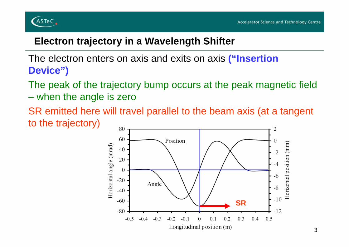
Electron trajectory in a Wavelength ShifterThe electron enters on axis and exits on axis (“Insertion Device”)The peak of the trajectory bump occurs at the peak magnetic field – when the angle is zeroSR emitted here will travel parallel to the beam axis (at a tangent to the trajectory)

SR

4

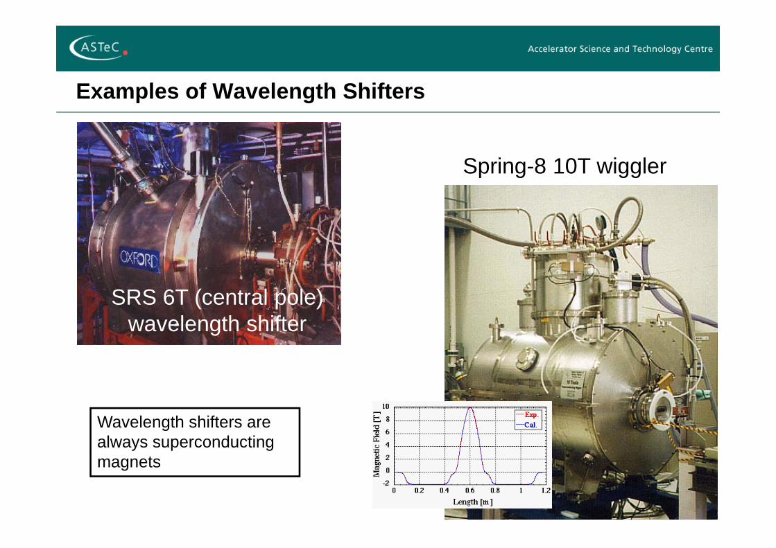
Examples of Wavelength Shifters

SRS 6T (central pole) wavelength shifter

Spring-8 10T wiggler

Wavelength shifters are always superconducting magnets

5

Extension to Multipole Wigglers

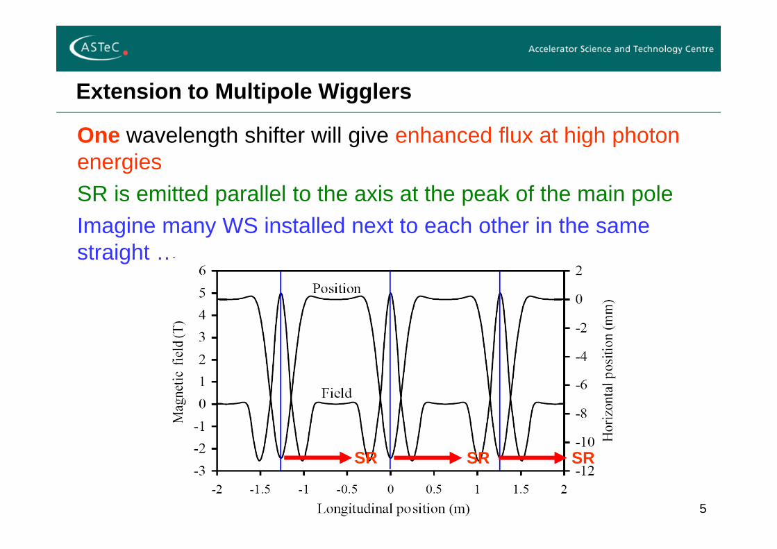
One wavelength shifter will give enhanced flux at high photon energiesSR is emitted parallel to the axis at the peak of the main poleImagine many WS installed next to each other in the same straight …

SRSR SR

6

Multiple Wavelength Shifters

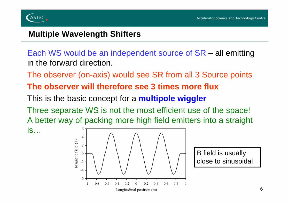
Each WS would be an independent source of SR – all emitting in the forward direction.The observer (on-axis) would see SR from all 3 Source pointsThe observer will therefore see 3 times more fluxThis is the basic concept for a multipole wigglerThree separate WS is not the most efficient use of the space!A better way of packing more high field emitters into a straight is…

B field is usually close to sinusoidal

7

Multipole Wigglers – Electron Trajectory

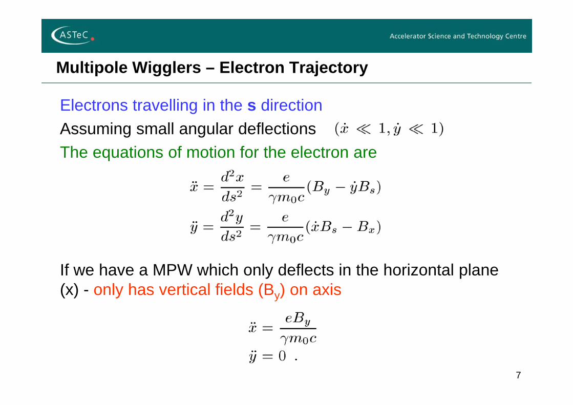
Electrons travelling in the s directionAssuming small angular deflectionsThe equations of motion for the electron are

If we have a MPW which only deflects in the horizontal plane (x) - only has vertical fields (By) on axis

8

Angular Deflection

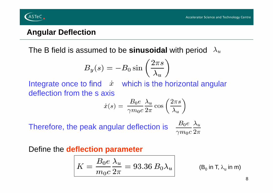
The B field is assumed to be sinusoidal with period

Integrate once to find which is the horizontal angular deflection from the s axis

Therefore, the peak angular deflection is

Define the deflection parameter

(B0 in T, u in m)

9

Trajectory

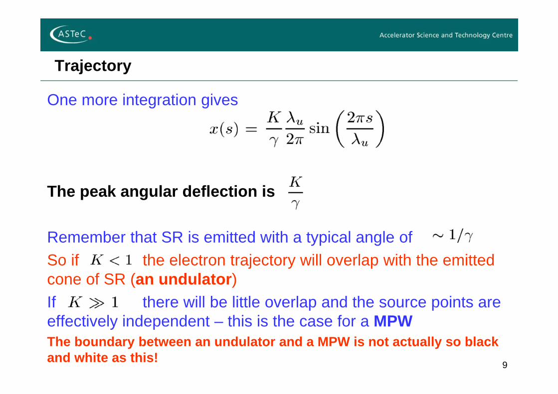
One more integration gives

The peak angular deflection is

Remember that SR is emitted with a typical angle ofSo if the electron trajectory will overlap with the emitted cone of SR (an undulator)If there will be little overlap and the source points are effectively independent – this is the case for a MPWThe boundary between an undulator and a MPW is not actually so black and white as this!

10

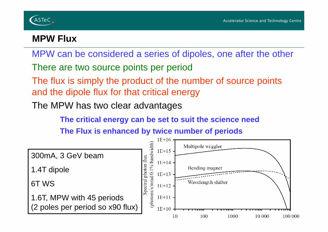
MPW FluxMPW can be considered a series of dipoles, one after the otherThere are two source points per periodThe flux is simply the product of the number of source points and the dipole flux for that critical energyThe MPW has two clear advantages

The critical energy can be set to suit the science needThe Flux is enhanced by twice number of periods

300mA, 3 GeV beam

1.4T dipole

6T WS

1.6T, MPW with 45 periods(2 poles per period so x90 flux)

11

MPW Power

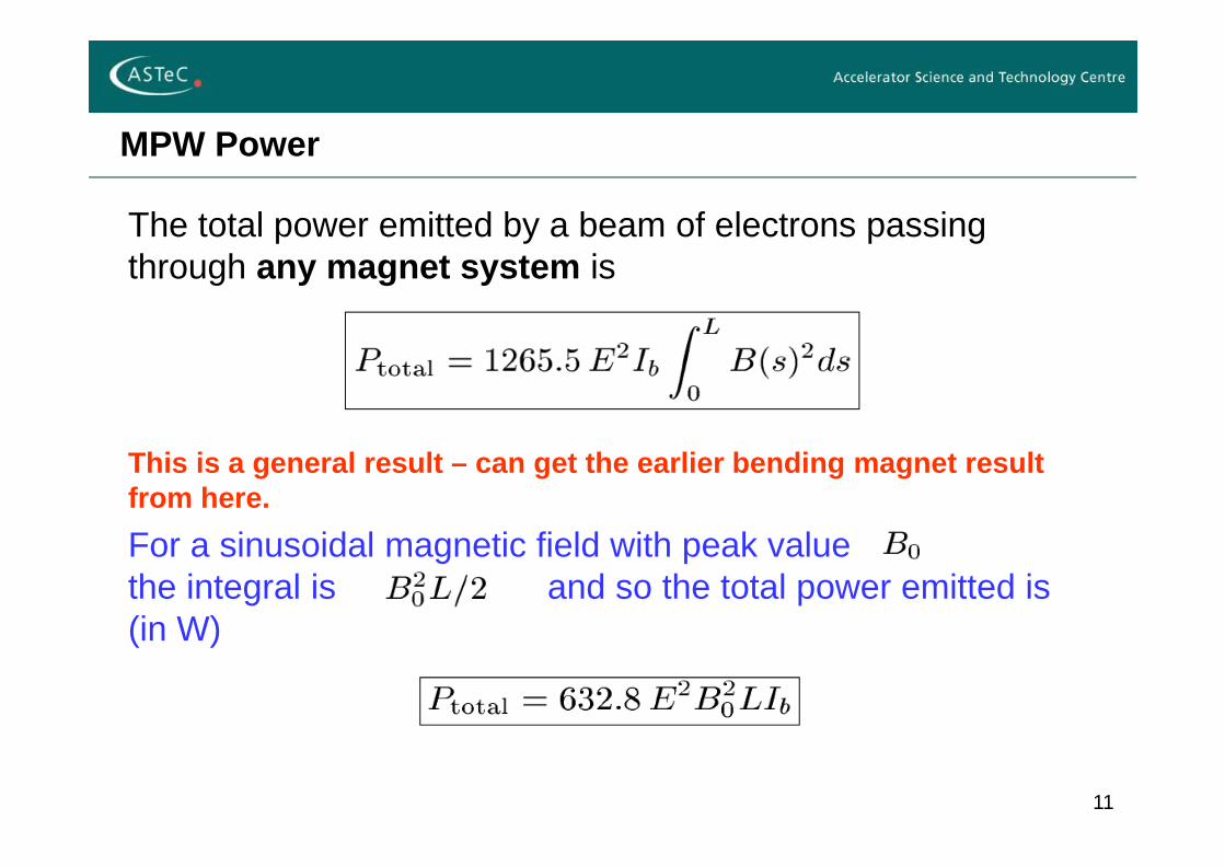
The total power emitted by a beam of electrons passing through any magnet system is

This is a general result – can get the earlier bending magnet result from here.For a sinusoidal magnetic field with peak value the integral is and so the total power emitted is (in W)

12

Power Density

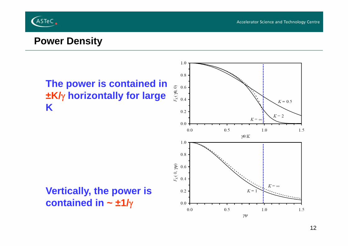
The power is contained in ±K/ horizontally for large K

Vertically, the power is contained in ~ ±1/

13

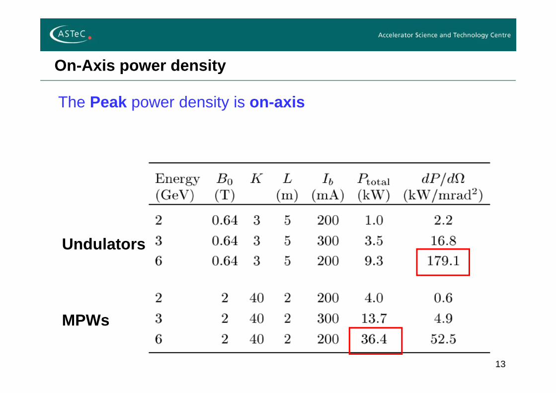
On-Axis power density

The Peak power density is on-axis

Undulators

MPWs

14

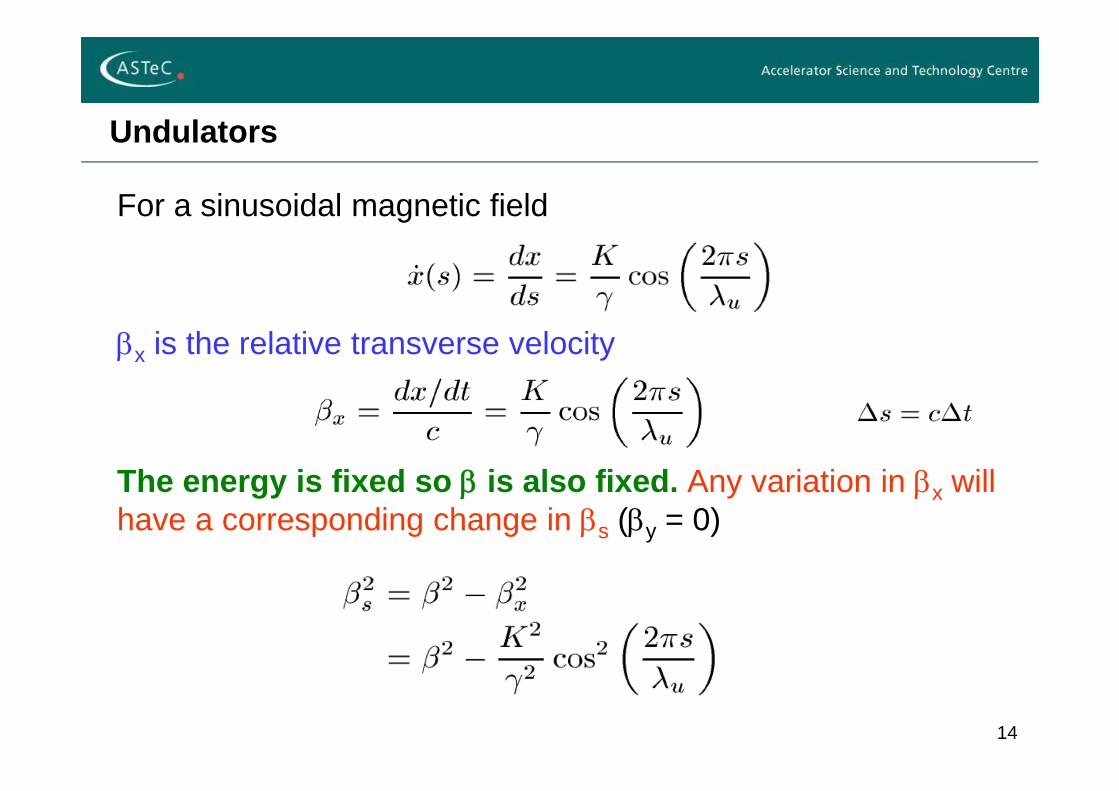
Undulators

For a sinusoidal magnetic field

x is the relative transverse velocity

The energy is fixed so is also fixed. Any variation in x will have a corresponding change in s (y = 0)

15

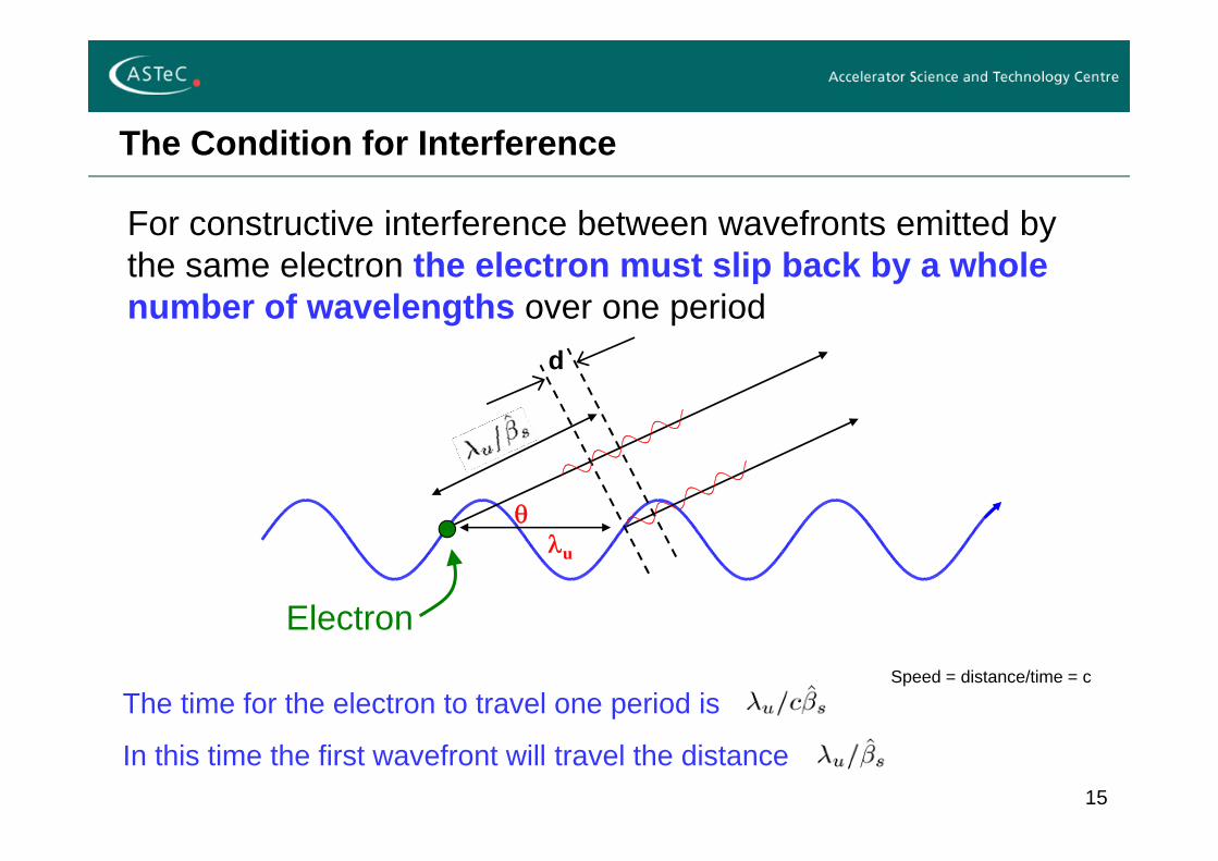
The Condition for Interference

For constructive interference between wavefronts emitted by the same electron the electron must slip back by a whole number of wavelengths over one period

The time for the electron to travel one period is

In this time the first wavefront will travel the distance

Speed = distance/time = c

Electron

d

u

16

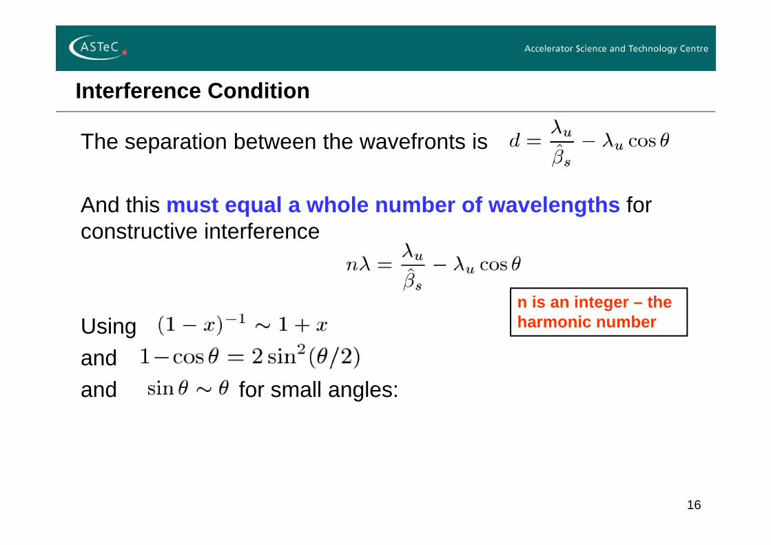
Interference Condition

The separation between the wavefronts is

And this must equal a whole number of wavelengths for constructive interference

Usingandand for small angles:

n is an integer – the harmonic number

17

Interference Condition

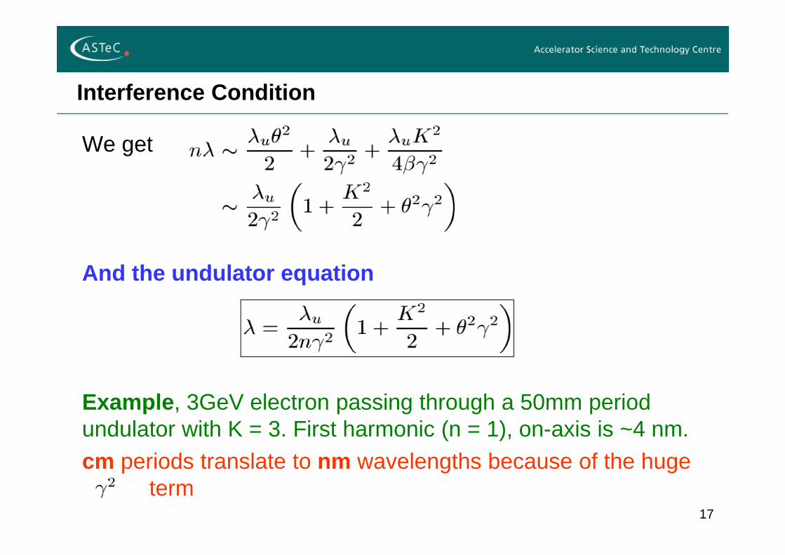
We get

And the undulator equation

Example, 3GeV electron passing through a 50mm period undulator with K = 3. First harmonic (n = 1), on-axis is ~4 nm.cm periods translate to nm wavelengths because of the huge

term

18

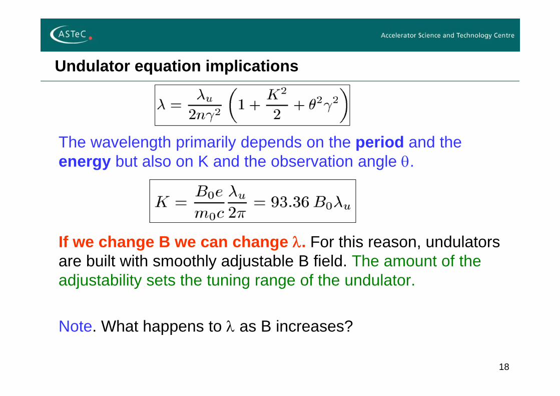
Undulator equation implications

The wavelength primarily depends on the period and the energy but also on K and the observation angle .

If we change B we can change . For this reason, undulators are built with smoothly adjustable B field. The amount of the adjustability sets the tuning range of the undulator.

Note. What happens to as B increases?

19

Undulator equation implications

As B increases (and so K), the output wavelength increases(photon energy decreases). This appears different to bending magnets and wigglers where we increase B so as to produce shorter wavelengths (higher photon energies).

The wavelength changes with 2, so it always gets longer as you move away from the axisAn important consequence of this is that the beamline aperture choice is important because it alters the radiation characteristics reaching the observer.

20

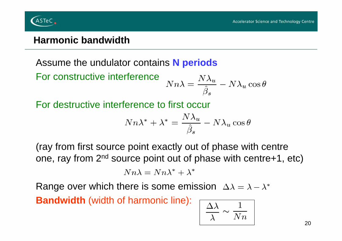
Harmonic bandwidth

Assume the undulator contains N periodsFor constructive interference

For destructive interference to first occur

(ray from first source point exactly out of phase with centre one, ray from 2nd source point out of phase with centre+1, etc)

Range over which there is some emissionBandwidth (width of harmonic line):

21

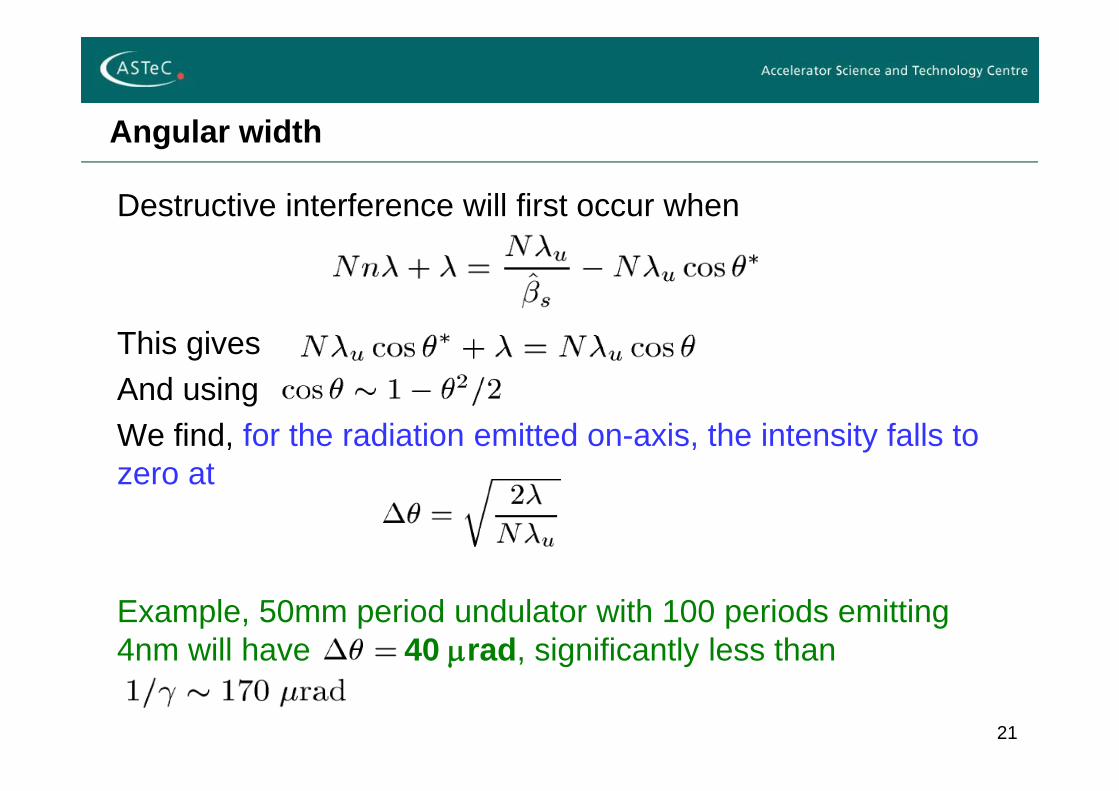
Angular width

Destructive interference will first occur when

This givesAnd usingWe find, for the radiation emitted on-axis, the intensity falls to zero at

Example, 50mm period undulator with 100 periods emitting 4nm will have 40 rad, significantly less than

22

Diffraction Gratings

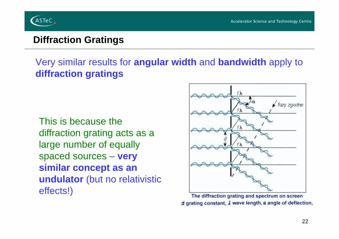
Very similar results for angular width and bandwidth apply to diffraction gratings

This is because the diffraction grating acts as a large number of equally spaced sources – very similar concept as an undulator (but no relativistic effects!)

23

When does an undulator become a wiggler?

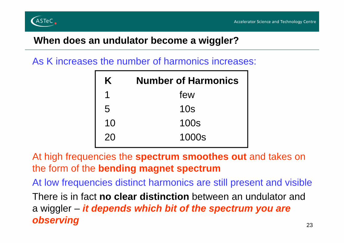
As K increases the number of harmonics increases:

K Number of Harmonics1 few5 10s10 100s20 1000s

At high frequencies the spectrum smoothes out and takes on the form of the bending magnet spectrumAt low frequencies distinct harmonics are still present and visibleThere is in fact no clear distinction between an undulator and a wiggler – it depends which bit of the spectrum you are observing

24

Undulator or Wiggler?

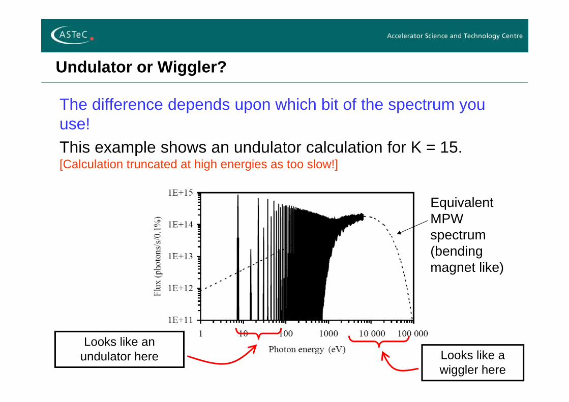
The difference depends upon which bit of the spectrum you use!This example shows an undulator calculation for K = 15. [Calculation truncated at high energies as too slow!]

Equivalent MPW spectrum (bending magnet like)

Looks like an undulator here Looks like a

wiggler here

25

Angular Flux Density

We want to gain an appreciation for the emitted radiation from an undulatorOne useful parameter is the (angular) flux density (photons per solid angle) as a function of observation angleLater we will look at the flux levels and also the polarisation of the radiation

26

n = 1n = 3

n = 4n = 2

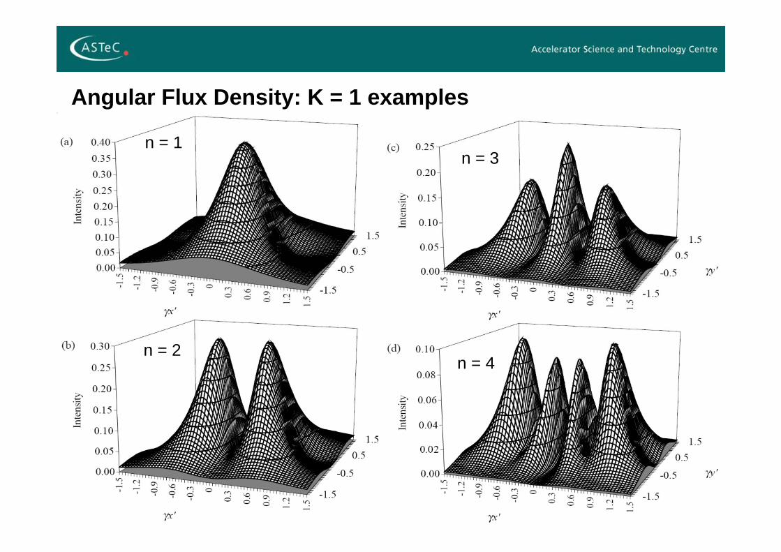
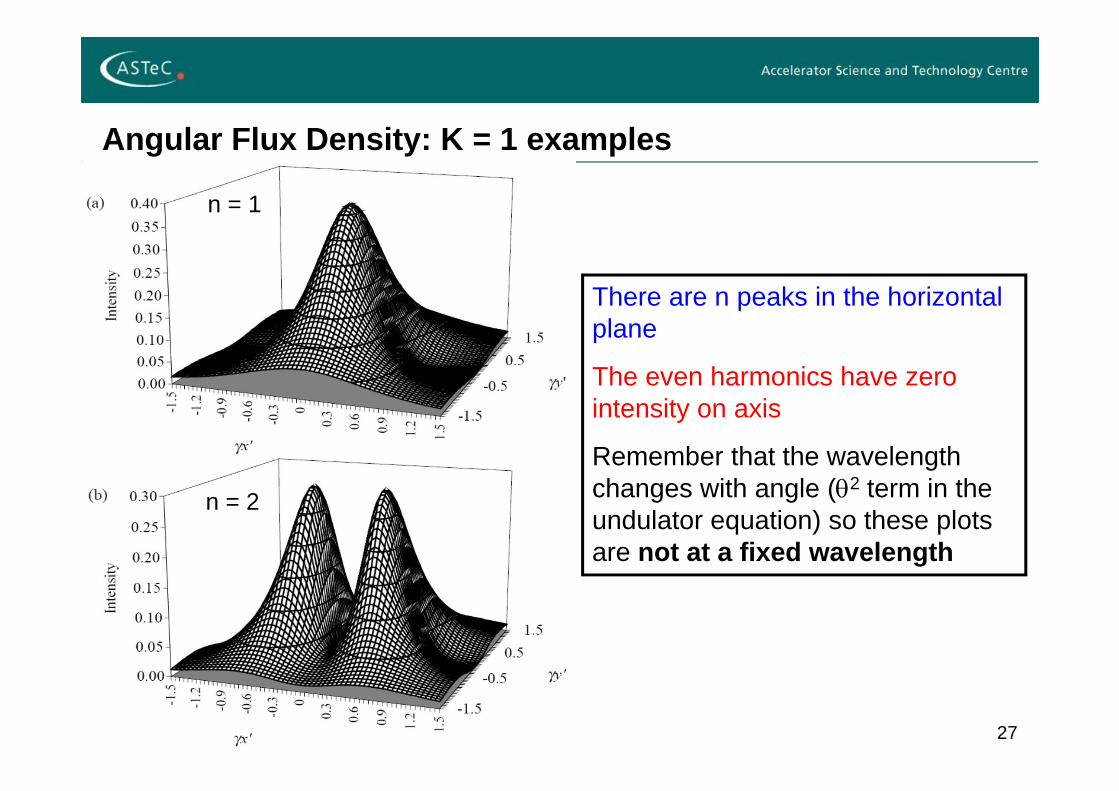
Angular Flux Density: K = 1 examples

27

n = 1

n = 2

There are n peaks in the horizontal plane

The even harmonics have zero intensity on axis

Remember that the wavelength changes with angle (2 term in the undulator equation) so these plots are not at a fixed wavelength

Angular Flux Density: K = 1 examples

28

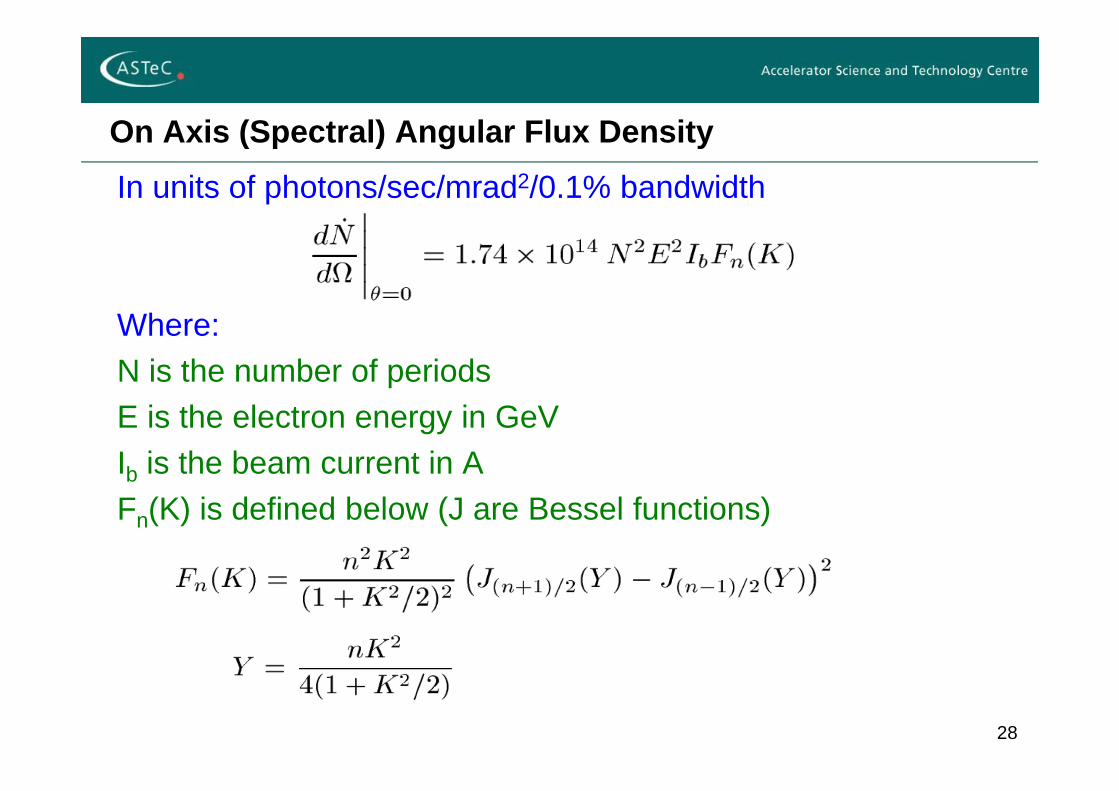
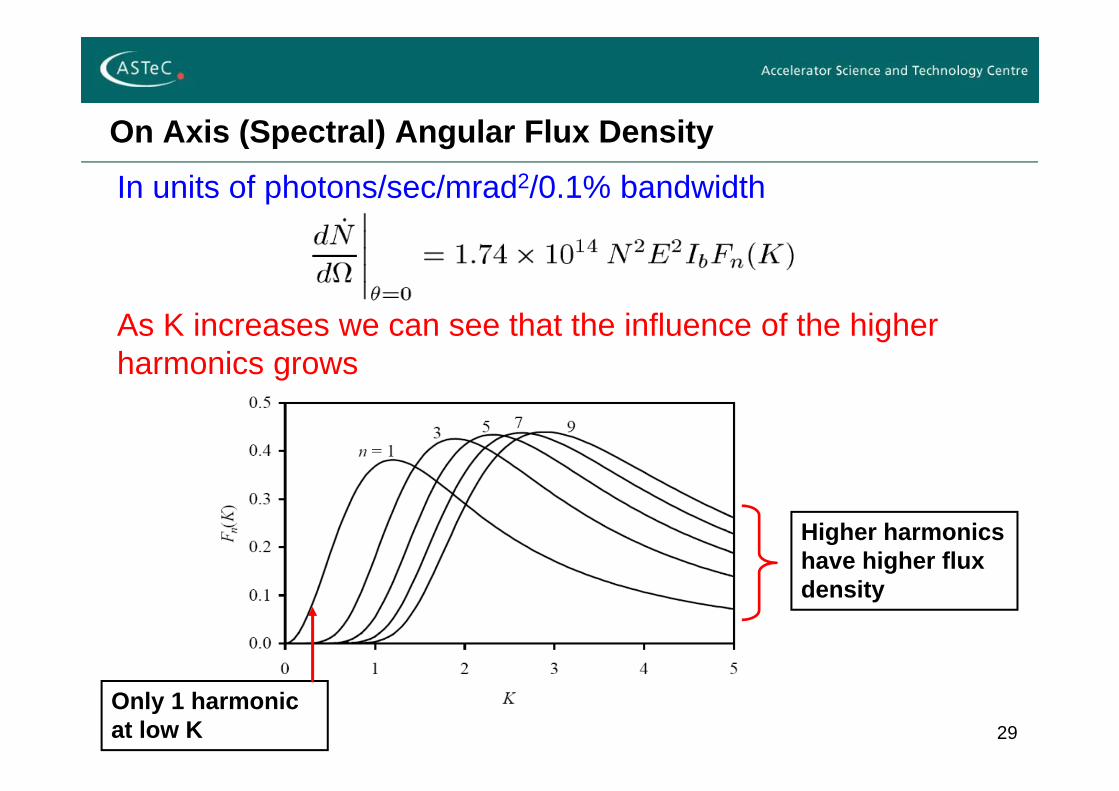
On Axis (Spectral) Angular Flux DensityIn units of photons/sec/mrad2/0.1% bandwidth

Where:N is the number of periodsE is the electron energy in GeVIb is the beam current in AFn(K) is defined below (J are Bessel functions)

29

On Axis (Spectral) Angular Flux DensityIn units of photons/sec/mrad2/0.1% bandwidth

As K increases we can see that the influence of the higher harmonics grows

Only 1 harmonic at low K

Higher harmonics have higher flux density

30

Example On Axis Angular Flux Density

An Undulator with 50mm period and 100 periods with a3GeV, 300mA electron beam will generate:Angular flux density of 8 x 1017 photons/sec/mrad2/0.1% bw

For a bending magnet with the same electron beam we get a value of ~ 5 x 1013 photons/sec/mrad2/0.1% bw

The undulator has a flux density ~10,000 times greater than a bending magnet due to the N2 term

31

Flux on-axis

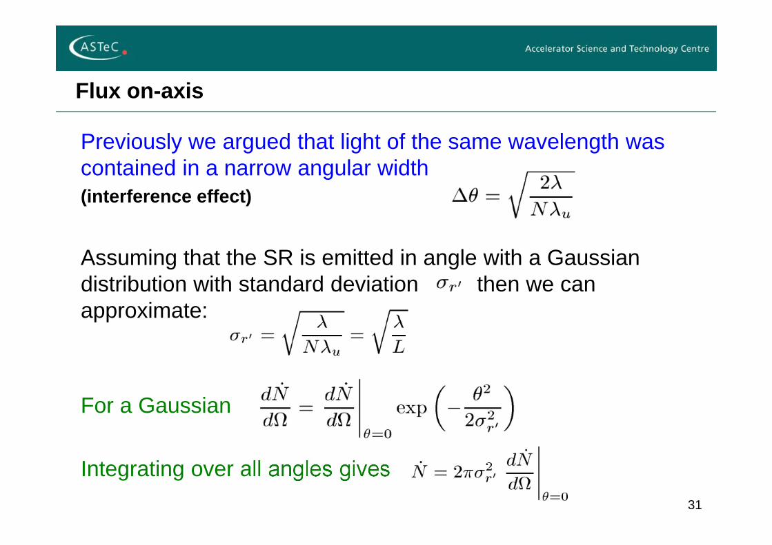
Previously we argued that light of the same wavelength was contained in a narrow angular width(interference effect)

Assuming that the SR is emitted in angle with a Gaussian distribution with standard deviation then we can approximate:

For a Gaussian

Integrating over all angles gives

32

Flux in the Central Cone

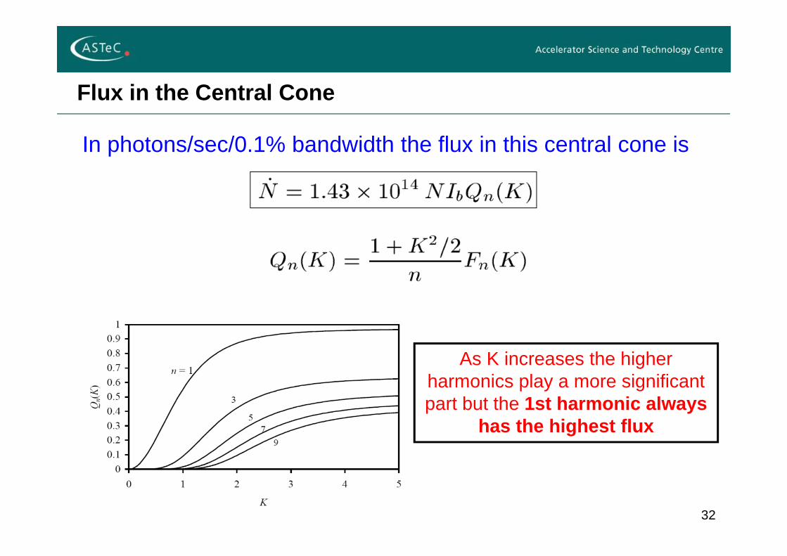
In photons/sec/0.1% bandwidth the flux in this central cone is

As K increases the higher harmonics play a more significant part but the 1st harmonic always

has the highest flux

33

Example Flux in the Central Cone

Undulator with 50mm period, 100 periods3GeV, 300mA electron beamOur example undulator has a flux of 4 x 1015 compared with the bending magnet of ~ 1013

The factor of few 100 increase is dominated by the number of periods, N (100 here)

34

Undulator Tuning Curves

Undulators are often described by “tuning curves”These show the flux (or brightness) envelope for an undulator.The tuning of the undulator is achieved by varying the K parameterObviously K can only be one value at a time !These curves represent what the undulator is capable of as the K parameter is varied – but not all of this radiation is available at the same time!

35

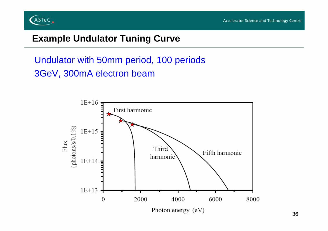
Example Undulator Tuning Curve

Undulator with 50mm period, 100 periods3GeV, 300mA electron beam

36

Example Undulator Tuning Curve

Undulator with 50mm period, 100 periods3GeV, 300mA electron beam

37

Example Undulator Tuning Curve

Undulator with 50mm period, 100 periods3GeV, 300mA electron beam

38

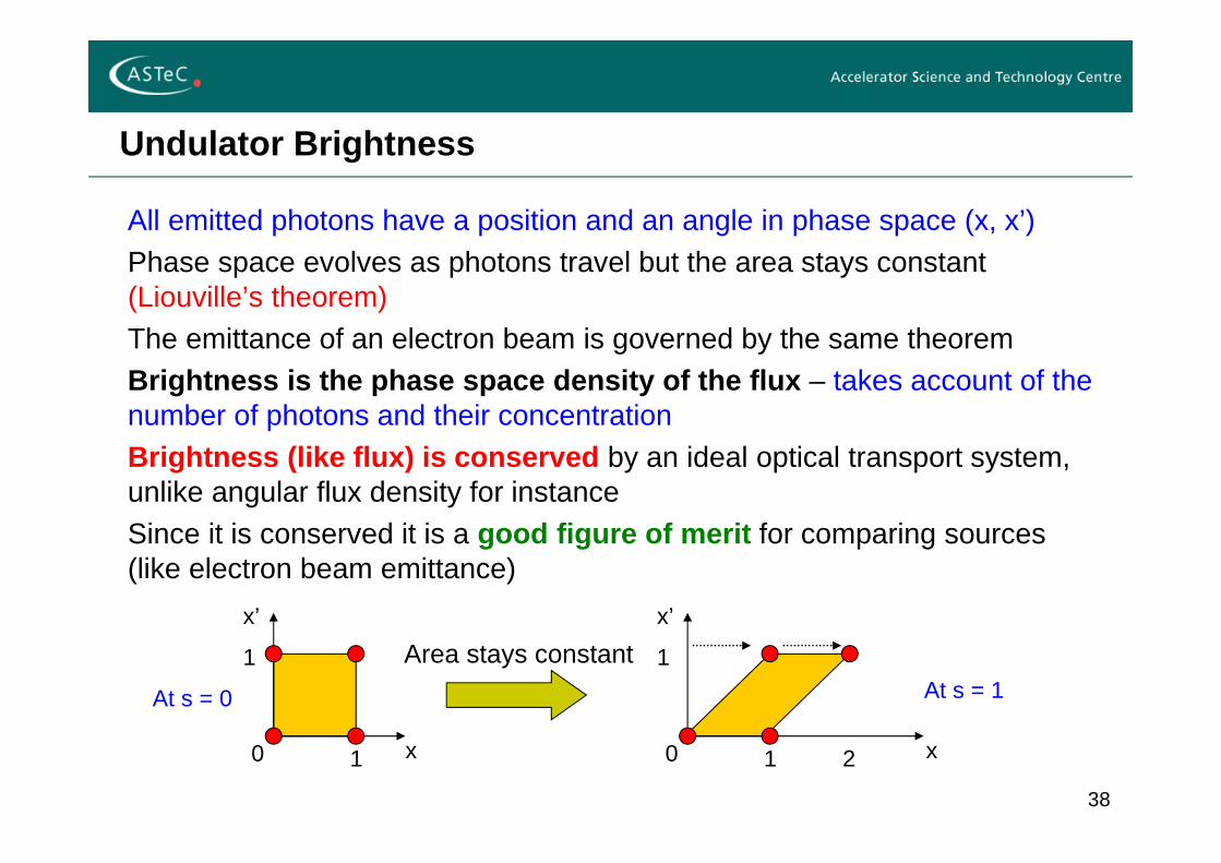
Undulator Brightness

All emitted photons have a position and an angle in phase space (x, x’)Phase space evolves as photons travel but the area stays constant (Liouville’s theorem)The emittance of an electron beam is governed by the same theoremBrightness is the phase space density of the flux – takes account of the number of photons and their concentrationBrightness (like flux) is conserved by an ideal optical transport system, unlike angular flux density for instanceSince it is conserved it is a good figure of merit for comparing sources (like electron beam emittance)

x0 1

x’

1

At s = 0

x0 1

x’

1

2

At s = 1Area stays constant

39

Undulator Brightness

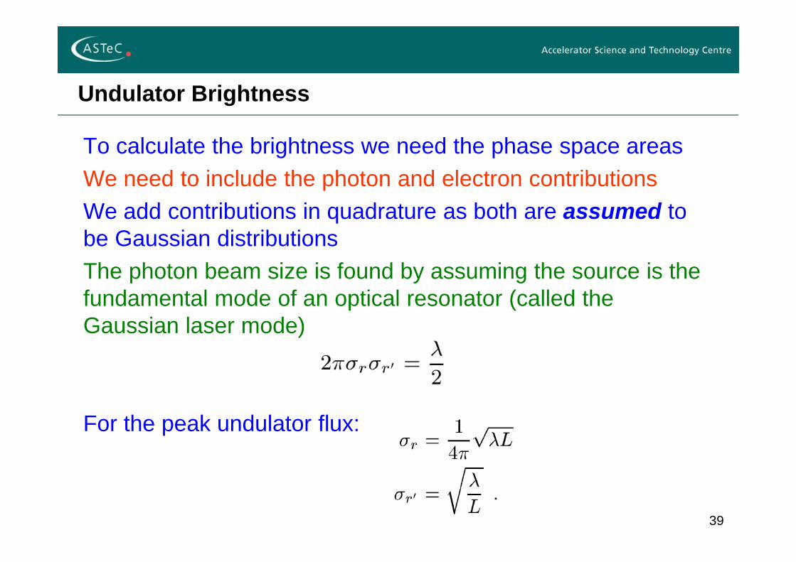
To calculate the brightness we need the phase space areasWe need to include the photon and electron contributionsWe add contributions in quadrature as both are assumed to be Gaussian distributionsThe photon beam size is found by assuming the source is the fundamental mode of an optical resonator (called the Gaussian laser mode)

For the peak undulator flux:

40

Undulator Brightness

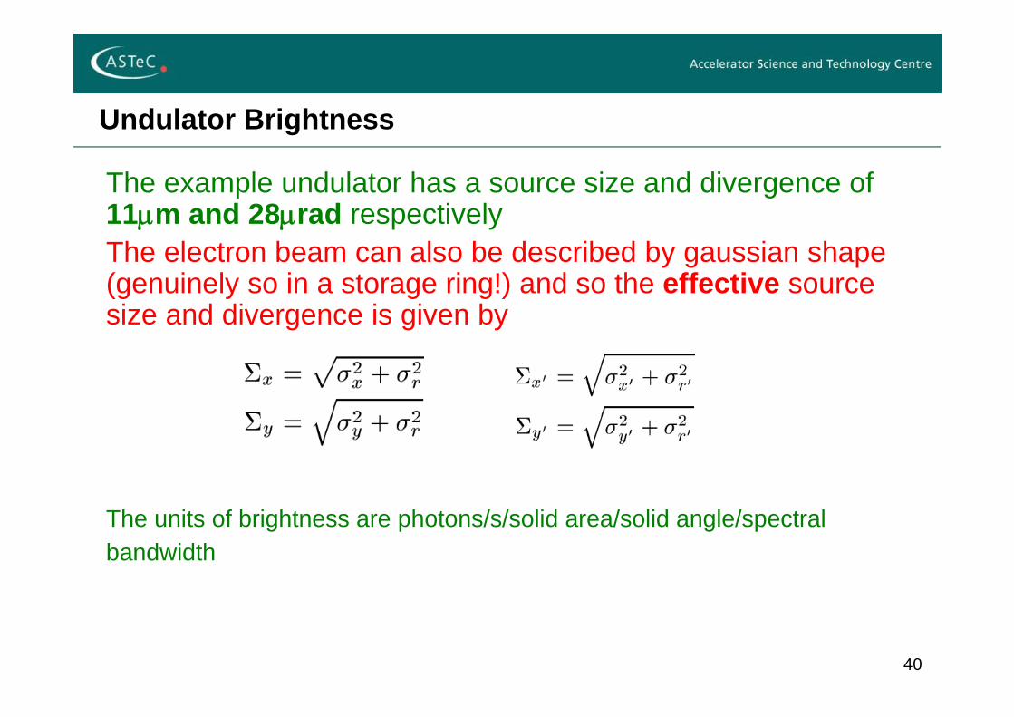
The example undulator has a source size and divergence of 11m and 28rad respectivelyThe electron beam can also be described by gaussian shape (genuinely so in a storage ring!) and so the effective source size and divergence is given by

The units of brightness are photons/s/solid area/solid angle/spectral bandwidth

41

Example Brightness

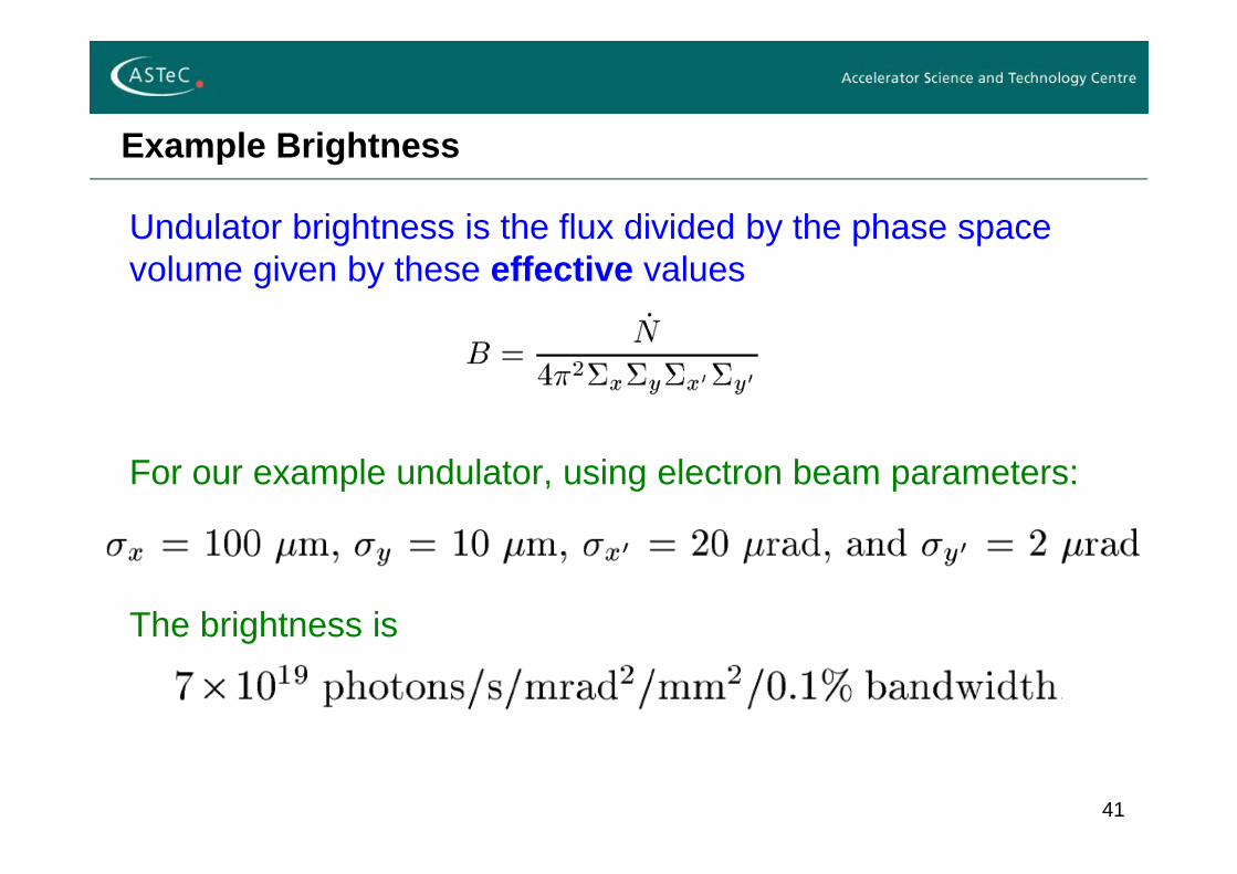
Undulator brightness is the flux divided by the phase space volume given by these effective values

For our example undulator, using electron beam parameters:

The brightness is

42

Brightness Tuning Curve

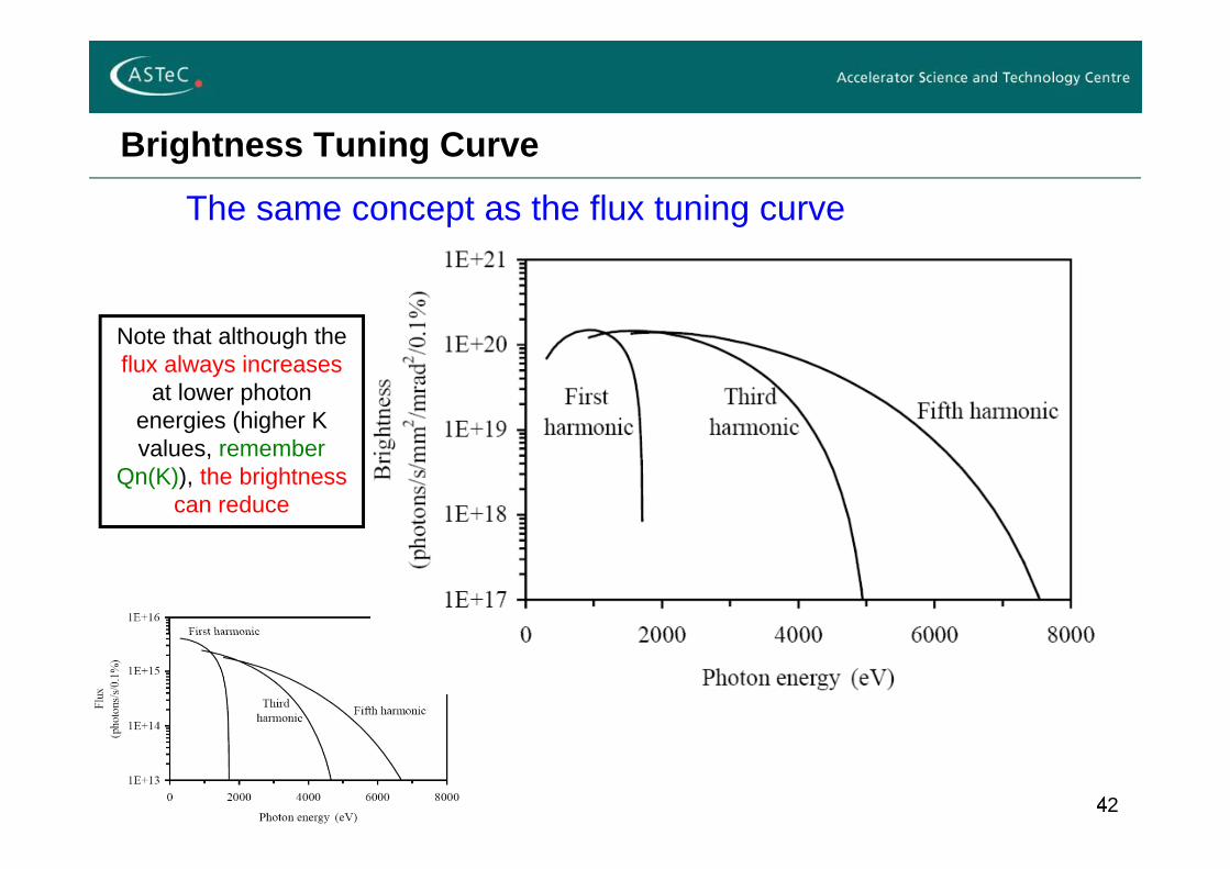
The same concept as the flux tuning curve

Note that although the flux always increases

at lower photon energies (higher K values, remember

Qn(K)), the brightness can reduce

43

Warning!

The definition of the photon source size and divergence is somewhat arbitraryMany alternative expressions are used – for instance we could have used

The actual effect on the absolute brightness levels of these alternatives is relatively smallBut when comparing your undulator against other sources it is important to know which expressions have been assumed !

44

Summary

Insertion Devices are added to accelerators to produce light that is specifically tailored to the experimental requirements(wavelength, flux, brightness, polarisation, …)Multipole wigglers are periodic, high field devices, used to generate enhanced flux levels (proportional to the number of poles)Undulators are periodic, low(er) field, devices which generate radiation at specific harmonicsThe distinction between undulators and multipole wigglers is not black and white. Undulator flux scales with N, flux density with N2