Insert here your thesis’ task.

Czech Technical University in Prague

Faculty of Electrical Engineering

Department of Computer Science

Master’s thesis

Exploiting betting market inefficiencies

with machine learning

Bc. Ondrej Hubacek

Supervisor: Ing. Gustav Sourek

7th January 2017

Acknowledgements

I would like to express my gratitude to my supervisor Gustav Sourek for his invaluableconsultations and persisting optimism.

In addition, I thank Assistant Professor Erik Strumbelj from the University of Ljubljana,for provided data.

Computational resources were provided by the CESNET LM2015042 and the CERITScientific Cloud LM2015085, provided under the programme “Projects of Large Re-search, Development, and Innovations Infrastructures”

Last but not least, I would like to thank all of my family for their continued supportduring my studies.

Declaration

I hereby declare that the presented thesis is my own work and that I have cited all sourcesof information in accordance with the Guideline for adhering to ethical principles whenelaborating an academic final thesis.

I acknowledge that my thesis is subject to the rights and obligations stipulated by theAct No. 121/2000 Coll., the Copyright Act, as amended, in particular that the CzechTechnical University in Prague has the right to conclude a license agreement on theutilization of this thesis as school work under the provisions of Article 60(1) of the Act.

In Prague on 7th January 2017 . . . . . . . . . . . . . . . . . . . . .

Czech Technical University in PragueFaculty of Electrical Engineeringc© 2017 Ondrej Hubacek. All rights reserved.

This thesis is school work as defined by Copyright Act of the Czech Republic. It has beensubmitted at Czech Technical University in Prague, Faculty of Electrical Engineering.The thesis is protected by the Copyright Act and its usage without author’s permissionis prohibited (with exceptions defined by the Copyright Act).

Citation of this thesis

Hubacek, Ondrej. Exploiting betting market inefficiencies with machine learning. Mas-ter’s thesis. Czech Technical University in Prague, Faculty of Electrical Engineering,2017.

Abstrakt

Cılem nası prace bylo najıt zpusob, jak profitovat na sazkarskem trhu pomocı stro-joveho ucenı. Zatımco vedecke prace se v minulosti hojne venovaly otazce, zda lzevytvorit model, ktery bude presnejsı nez bookmaker, ziskovosti modelu nebyla venovanadostatecna pozornost. Tvrdıme, ze zisk nenı dusledkem pouze samotne presnosti. Mıstotoho navrhujeme dekorelaci od predikcı bookmakera, stale vsak nezapomınaje na presnostpredikce. Dale predstavujeme inovativnı prıstup k agregaci statistik hracu pomocıkonvolucnıch neuronovych sıtı. V neposlednı rade ukazujeme vyuzitı ”Modern Port-folio Theory“, matematickeho ramce pro optimalizaci portfolia, v kontextu sazenı proporovnavanı ruznych sazecıch strategiı. Nami navrzene modely byly v souhrnu 15 sezonNBA ziskove. Nenı nam znamo, ze by doposud byla zverejnena prace podobneho rozsahu.

Klıcova slova prediktivnı modelovanı, sportovnı analyza, sazkarske trhy, neuronovesıte, basketbal

ix

Abstract

The goal of our work was to find a way to profit from betting market using machinelearning. While a lot of research has been devoted to determining whether a bookmakercan be beaten in terms of accuracy, surprisingly little attention was paid to evaluatingthe profitability of statistical models over the bookmaker. We argue that the profit isnot solely affected by the models’ accuracy. Instead, we encourage decorrelation of themodels’ output from the bookmaker’s predictions, while keeping the accuracy reasonablyhigh. Moreover, we introduce a novel approach of aggregating player-level statisticsusing convolutional neural networks. Last but not least, we illustrate the use of ModernPortfolio Theory, a mathematical framework for portfolio optimization, in the context ofbetting for comparison of diverse betting strategies. Our proposed models were able toachieve a positive profit totaling over the course of 15 NBA seasons. To the best of ourknowledge, no work of similar scale has been done and made publicly available before.

Keywords predictive modeling, sports analytics, betting markets, neural networks,basketball

x

Contents

1 Introduction 1

1.1 Problem Statement . . . . . . . . . . . . . . . . . . . . . . . . . . . . . . . 1

1.2 Betting Markets . . . . . . . . . . . . . . . . . . . . . . . . . . . . . . . . 1

1.3 National Basketball Association . . . . . . . . . . . . . . . . . . . . . . . . 4

1.4 Predictive Modeling . . . . . . . . . . . . . . . . . . . . . . . . . . . . . . 5

2 Literature Review 11

2.1 Betting Markets . . . . . . . . . . . . . . . . . . . . . . . . . . . . . . . . 11

2.2 Human vs Machine . . . . . . . . . . . . . . . . . . . . . . . . . . . . . . . 12

2.3 Predictive Models . . . . . . . . . . . . . . . . . . . . . . . . . . . . . . . . 14

2.4 Features . . . . . . . . . . . . . . . . . . . . . . . . . . . . . . . . . . . . . 17

3 Analysis and Design 19

3.1 Gathering Data . . . . . . . . . . . . . . . . . . . . . . . . . . . . . . . . . 19

3.2 Building Datasets . . . . . . . . . . . . . . . . . . . . . . . . . . . . . . . . 19

3.3 Exploratory Data Analysis of Bookmakers’ Odds . . . . . . . . . . . . . . 20

3.4 Predictive Modeling . . . . . . . . . . . . . . . . . . . . . . . . . . . . . . 23

3.5 Betting Strategies . . . . . . . . . . . . . . . . . . . . . . . . . . . . . . . 26

4 Experiments 33

4.1 Simulation of the Betting Strategy . . . . . . . . . . . . . . . . . . . . . . 33

4.2 Model Evaluation . . . . . . . . . . . . . . . . . . . . . . . . . . . . . . . . 35

4.3 Comparison with State-of-the-art . . . . . . . . . . . . . . . . . . . . . . . 47

5 Conclusion 49

5.1 Future Work . . . . . . . . . . . . . . . . . . . . . . . . . . . . . . . . . . 50

Bibliography 51

A Features’ descriptions 55

xi

B Acronyms 61

C Contents of enclosed CD 63

xii

List of Figures

1.1 A schema of a neuron . . . . . . . . . . . . . . . . . . . . . . . . . . . . . . . 61.2 A schema of an ANN . . . . . . . . . . . . . . . . . . . . . . . . . . . . . . . . 71.3 Examples of activation functions . . . . . . . . . . . . . . . . . . . . . . . . . 8

3.1 Distribution of odds set by the bookmaker for home team (left) and forvisiting team (right). . . . . . . . . . . . . . . . . . . . . . . . . . . . . . . . . 21

3.2 Margin distribution over the seasons . . . . . . . . . . . . . . . . . . . . . . . 223.3 Margin distribution conditioned by the bookmaker’s odds . . . . . . . . . . . 223.4 Estimates of P (win,COURT |ODDS) (left) and P (win|ODDS) (right). . . . 233.5 PDFs of P (BOOK,COURT ) and P (BOOK,COURT |win) . . . . . . . . . . 243.6 Estimate of P (win|ODDS) from data with margin and with stripped margin 253.7 Risk-expected return space with random strategies and efficient frontier . . . 303.8 Comparison of the betting strategies in the risk-return space . . . . . . . . . 31

4.1 Accuracy of the ANN and LR models over seasons 2000–2014 . . . . . . . . . 374.2 Correlation between the ANN model and bookmaker’s predictions . . . . . . 374.3 Comparison of models’ profitability using the proposed (left) and fixbet (right)

betting strategies. . . . . . . . . . . . . . . . . . . . . . . . . . . . . . . . . . 384.4 Analysis of predictions of models trained with sample weighting . . . . . . . . 404.5 Comparison of models’ profitability using proposed (left) and fixbet (right)

betting strategy . . . . . . . . . . . . . . . . . . . . . . . . . . . . . . . . . . . 404.6 Analysis of predictions of the ANN model trained with the decorrelation term

in loss function for varying values of c . . . . . . . . . . . . . . . . . . . . . . 424.7 Distribution of P (win|away, c, F ) for different values of c . . . . . . . . . . . 434.8 Analysis of predictions of the thresholded models . . . . . . . . . . . . . . . . 444.9 Accuracy of the ANN and ANN player models in seasons 2000–2014 . . . . . 454.10 Correlation between the ANN player model and bookmaker’s predictions . . 464.11 Comparison of models’ profitability using proposed (left) and fixbet (right)

betting strategy . . . . . . . . . . . . . . . . . . . . . . . . . . . . . . . . . . . 46

xiii

List of Tables

3.1 Meta-parameters of the used Models . . . . . . . . . . . . . . . . . . . . . . . 263.2 Comparison of betting strategies on simulated betting opportunities. . . . . . 31

4.1 Effects of the ground truth and model’s output distributions variances on theevaluation metrics . . . . . . . . . . . . . . . . . . . . . . . . . . . . . . . . . 34

4.2 Effects of different correlation levels between the true probabilities, the modeland the bookmaker on the evaluation metrics. . . . . . . . . . . . . . . . . . . 34

4.3 Number of games and bookmaker’s accuracy in each of the seasons . . . . . . 364.4 Mean results over the seasons of the LR and ANN model . . . . . . . . . . . 364.5 Results of ANN models trained with sample weighting . . . . . . . . . . . . . 394.6 Result of ANN model trained with the decorrelation term in loss function for

varying values of c . . . . . . . . . . . . . . . . . . . . . . . . . . . . . . . . . 414.7 Results of confidence thresholding of the team-level model . . . . . . . . . . . 424.8 Results of ANN player model . . . . . . . . . . . . . . . . . . . . . . . . . . . 454.9 Result of ANN player model trained with decorrelation term in loss function

with different values of c . . . . . . . . . . . . . . . . . . . . . . . . . . . . . . 474.10 Results of confidence thresholding of the player-level model . . . . . . . . . . 474.11 Comparison of accuracy of our models with state-of-the-art . . . . . . . . . . 48

xv

Chapter 1

Introduction

1.1 Problem Statement

Advances in machine learning allow us to tackle a variety of problems in diverse domains.I this work we focus on predictive sports analytics in the context of betting markets. Ourgoal is to exploit betting market inefficiencies, i.e. to profit from the market. Bettingmarkets thus serve for validation of our findings as well as a subject of our researchinquiry by themselves.

Since there are many sports events offered at the betting markets, identifying suitablesub-domain to apply our ideas on is a vital part of the thesis, too. Our approachis generally data-driven, therefore relevant historical data have to be aggregated andprocessed.

To assess the theoretical profits of the model, authentic simulation of betting has tobe implemented. The resulting evaluation criterion of the models’ is their profitability.Comparison with state-of-the-art w.r.t. the accuracy of the prediction is also desirable.

1.2 Betting Markets

Sports betting is the act of placing a wager on a subset of outcomes of random sportsevents, each of which is associated with a corresponding profit as predefined by a book-maker (Sec. 1.2.1). Such an assignment of bookmaker’s estimate to the random event’soutcome defines a betting opportunity. In the case of a correct identification of an out-come, the subject wins back the wager plus the profit or losing the wager otherwise. Thestructure of the outcomes and associated profits are based on various types of bets asdescribed in Sec. 1.2.3.

1.2.1 The Bookmakers

The bookmaker is a company or a person accepting wagers on various events of inherentstochastic nature. Historically the bookmakers operated betting shops, but with the

1

1. Introduction

expansion of the Internet, most bookmakers these days operate online through bettingsites. The goal of the bookmakers is to maximize their profits.

1.2.2 Prediction Markets

An alternative to a traditional bookmaker are the prediction markets in sports betting,also known as betting exchanges. In a betting exchange, there is not a single author-ity defining the odds. Instead, each participant can use the exchange to allow otherparticipants to bet against his odds. The betting exchange is in some way similar to afinancial market. Although we find betting exchanges very interesting, their complicatedstructure makes it harder to model their behavior and to reliably evaluate our model ina hypothetical scenario against the exchange. Therefore we evaluate our models againstthe bookmaker where such problems simply do not arise.

1.2.3 Types of Bets

Bookmakers these days offer a variety of betting opportunities. We describe the mostfrequent types in this subsection.

1.2.3.1 Moneyline Bets

To win a so called moneyline bet, predicting the winner of the game is required. Foreach of the outcomes, the bookmaker sets the corresponding odds. There are differentformats for representing the odds, too. In Europe, the most common one is the so-calleddecimal odds. For example, if bookmaker sets the odds to 1.8 for the home team to win,a bettor place a wager of 100 Eur and the home team actually wins, the bettor’s profitwill be 1.8× 100− 100 Eur.

1.2.3.2 Spread Betting

Bookmakers can assign spread, also called line, to handicap a team and favor its oppon-ent. For example, if the line is Home team -7.5 : Visiting team +7.5 and the bettorbets on the Home team, he wins when the home team beat its opponent by at least 8points.

In this work, we decided to use the moneyline betting format as, among the Europeanbookmakers, the moneyline bets are more common. Also, to reflect the spread bettingformat, we would have to switch from classification to regression, which would make thetask slightly more complicated.

1.2.3.3 Total Bets

Besides betting on the game outcome, one of the most popular bets are so called totalsor under/over bets. The goal of the bettor is to predict how many points (or goals etc.)will be scored in a game in total. For example, the most common under/over bet in

2

1.2. Betting Markets

soccer is under/over 2.5. Bettor has an option to bet under or over. If he bets over, andmore than 2 goals are scored, the bet is won.

Again, both moneyline bets and spread bets are feasible. In spread betting, thebettor’s winnings are based on how many goals or points were scored above the threshold.In moneyline betting, fixed odds are assigned for each threshold.

Had we decided to approach the task of predicting the outcome of the game asregression, we could have instantly obtained the prediction for under/over bets too.However finding historical odds or lines for under/over turned out to be very problematic.

1.2.3.4 Proposition Bets

The betting opportunities are almost limitless these days, and proposition bets are proofof that fact. Not only bettors can bet whether a particular player will score a goal in asoccer match or how many passes will the team successfully finish in the game, but alsohow many corners will occur in first 30 minutes or who will win the coin flip at the startof the game. Soccer match serves only for illustration here; the proposition bets are notlimited to a specific domain.

While some of the subjects of the proposition bets would be interesting to model,finding freely available historical odds for these events is not possible.

1.2.3.5 In-play Bets

Some online bookmakers offer the possibility to bet during the course of a game, whileupdating their odds according to the current situation inside the game. Although we findthis mode interesting, beating the in-play odds would require real-time data gatheringand evaluation, which would make the whole task much harder, and thus we focus solelyon the scenario of placing the bets before the actual start of a game.

1.2.4 Bookmaker’s Edge

In the gambling market, the operator usually has the advantage over the gamblers. Forexample in roulette, casino wins all bets in case the ball falls onto the number 0. Whilepoker is being mostly played among the players and not against the casino, the casinotakes a percentage of the placed bets in each hand - the so-called “rake”. In sportsbetting, bookmaker secures his edge by offering unfair odds.

A line for spread betting usually looks like this: Home team -7.5 : Visiting team+7.5 (-110). We have explained, what do the decimal numbers mean. The value -110relates to bookmaker’s edge. It implies, that to win 100 Eur, one has to bet 110. Inother words, the value represents ≈ 9% commission.

In moneyline betting, the bookmaker is slightly more devious. His edge is not thatobvious sometimes. If the odds being laid out were fair, the inverse odds could beinterpreted as the probability of the outcome estimated by the bookmaker. In practicefor example, when the bookmaker is indifferent which outcome is more probable, hedoes not set the fair odds as 2.0 − 2.0 but offers a lower portion of profit such as

3

1. Introduction

1.95−1.95. The absolute difference between the sum of true probabilities (1 by definition)and probabilities implied by inverted odds is called the margin. In our example, thebookmaker’s margin would be 1.95−1 + 1.95−1 − 1 ≈ 2.5%.

The presence of the margin becomes less apparent when the bookmaker is moreconfident about the game outcome, and the odds of one team to win are close to 1. Forexample, when bookmaker estimates winning chances of the team as 90 % against 10%, the fair odds would be 1.11, 10. If the bookmaker tweaks the odds at first sightmarginally in his favor, for example, 1.07 - 10, the margin would suddenly jump to≈ 3.5%

The size of the margin differs among bookmakers. The bookmaker has to optimizebetween the size of the margin and the number of customers. Should the odds on his sitebe consistently worse (lower) than on some other site, the bookmaker would quickly losehis customers. The market ensures that the margin is usually between 2 to 5 percent.Also, local laws can affect the market. Enforcing additional taxes forces bookmaker toincrease the margin or implement a commission from winnings. Banning foreign bettingsites takes options from bettors and allows local betting sites to get away with a highermargin than in the free market.

1.2.5 Arbitrage Betting

Arbitrage betting happens when a bettor makes use of bookmakers offering odds for thesame event. In rare cases, two bookmakers offer odds steered towards opposite outcomes.For example one bookmaker (A) can set odds for one game 1.4 and 3.3 while the otherbookmaker (B) lays down the odds as 1.3 and 4. If the bettor posses 100 Eur, he canmake a risk-free profit by betting 74 Eur on the home team at bookmaker A with odds1.4 and the remaining 26 Eur on the visiting team at bookmaker B with 4 odds. Thissplit ensures him profit about 3.7 Eur regardless of the result of the game.

Arbitrage betting looks very tempting on the paper. However, Franck; Verbeek;Nuesch, 2009 showed, that 98 % arbitrage bets lead to the profit of 1.2 % or lower.Moreover, to make such profit, the bettor would have to have his finances spread acrossmultiple betting sites to be able to catch the odds. These so called “sure bets” areimmediately identified and exploited by the market. Once the bettor would make sucha bet, he would be committed not only to winning the money at one of the betting sites,but also losing the whole bet at the other site he placed his bet. This would lead to aconstant need of moving money around, assuring that they are available at each bettingsite for next “sure bet” opportunities.

1.3 National Basketball Association

In order to design and evaluate forecasting model we needed to obtain both the data totrain our models and the bookmakers’ odds. We found out that NBA offers the mostcomprehensive sets of statistics, thus we decided to test our ideas on NBA.

4

1.4. Predictive Modeling

1.3.1 Structure

NBA is a men’s professional basketball league in North America founded 1946 currentlyplayed by 30 teams.

The teams are separated into the Western and the Eastern conferences. Moreover,each conference is divided into three divisions – the Eastern into Pacific, Central, South-east and the Western into Northwest, Southwest, Pacific. Each division contains 5 teams.82 are played in regular season. Each team plays other teams from the same division 4times, 6 teams from the other 2 divisions 4 times and remaining 6 teams from the sameconference 3 times. Teams from the second conference are faced 2 times.

A roster of each team consists of 15 players (12 active and 3 inactive). For each game,the coach can change active and inactive players. Active players are then available forthe game. 5 players from each of opposing teams are on the court simultaneously. Thenumber of substitutions is not limited. In late October rosters are locked. The tradedeadline is usually in February. Teams are not allowed to trade players, they may,however, sign or release players.

At the end of regular seasons 8 teams from each conference advance into playoffs.Playoffs are played in tournament format. Teams face their opponents in best of sevenseries – first one to win 4 games advances to next stage, loser is eliminated.

1.3.2 Data Available

There are several types of data recorded.

Box score data provide a summary of a game. Players’ and teams’ statistics (numberof shots, number of steals, ...) per game are recorded.

Play-by-play data represents a time-line of a game. Each event that happens in thegame (shot taken, steal, ...) is recorded with exact time.

Player tracking data are recorded using video tracking system. Position of the balland all players is recorded in short time intervals. While these data allow completereconstruction of the game, they are not freely available.

1.4 Predictive Modeling

The goal of predictive modeling is to build models capable of predicting outcomes ofevents, in our case the outcomes of sports matches, given some qualitative description ofthe events. Machine learning is about creating algorithms that can learn such predict-ive models while generalizing from training data, i.e. quantitative descriptions of thehistorical events.

There are various machine learning techniques available that might be used for thetask at hand. Artificial neural networks (ANNs) were our models of choice. The natureof ANNs allows us to tune the complexity of the models easily. This makes the ANNsvery scalable – if we were in need of adding additional features, the model structure

5

1. Introduction

could be tweaked in an appropriate manner. The data we are dealing with have arelational character. The architecture of the neural network allowed us to aggregate theplayer-level statistics using a convolutional or a locally connected layers.

In this section, we briefly introduce ANNs. Much more details can be found forexample in Goodfellow et al., 2016 and Orr et al., 2003.

Artificial neural network is a model inspired by the human brain. ANN consists of aset of highly interconnected units – neurons.

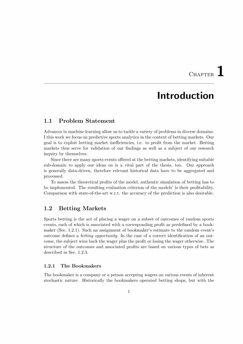
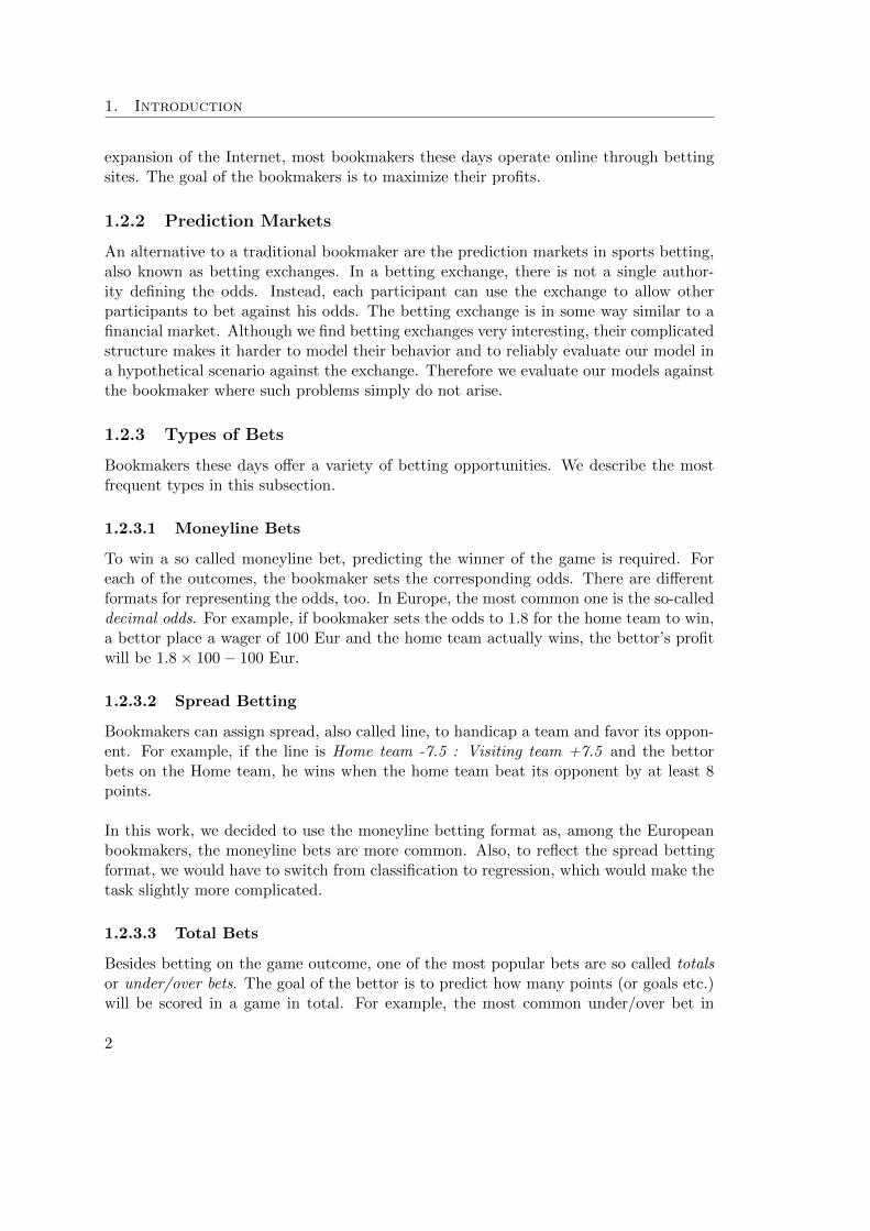
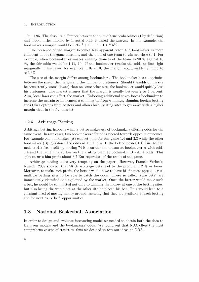
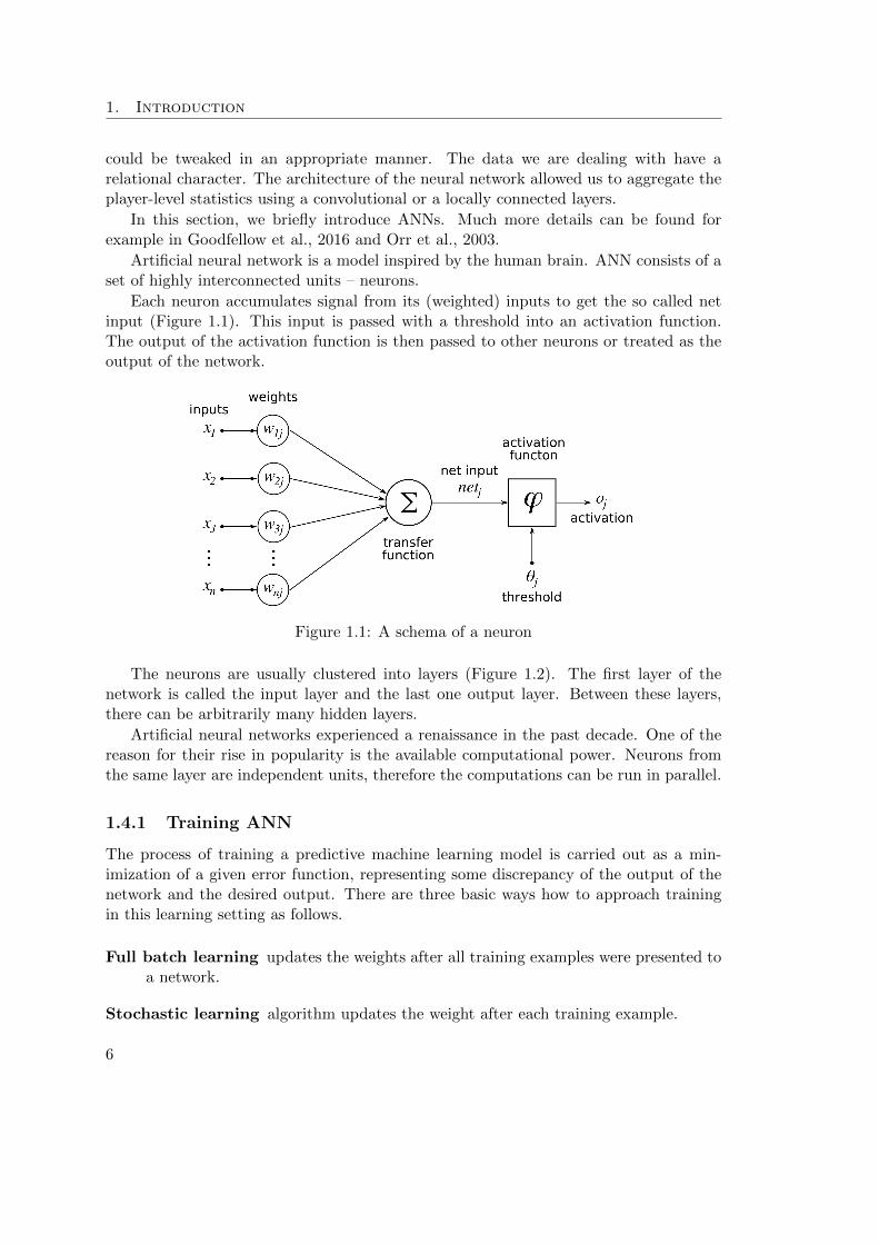
Each neuron accumulates signal from its (weighted) inputs to get the so called netinput (Figure 1.1). This input is passed with a threshold into an activation function.The output of the activation function is then passed to other neurons or treated as theoutput of the network.

Figure 1.1: A schema of a neuron

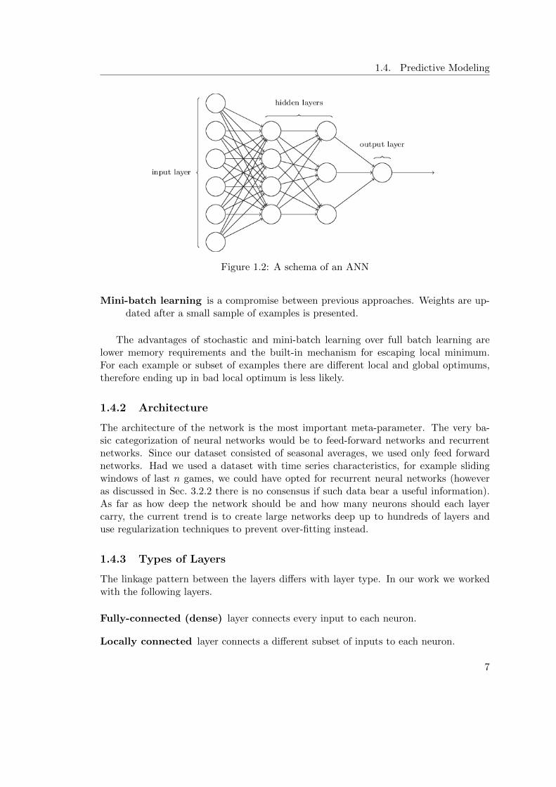
The neurons are usually clustered into layers (Figure 1.2). The first layer of thenetwork is called the input layer and the last one output layer. Between these layers,there can be arbitrarily many hidden layers.

Artificial neural networks experienced a renaissance in the past decade. One of thereason for their rise in popularity is the available computational power. Neurons fromthe same layer are independent units, therefore the computations can be run in parallel.

1.4.1 Training ANN

The process of training a predictive machine learning model is carried out as a min-imization of a given error function, representing some discrepancy of the output of thenetwork and the desired output. There are three basic ways how to approach trainingin this learning setting as follows.

Full batch learning updates the weights after all training examples were presented toa network.

Stochastic learning algorithm updates the weight after each training example.

6

1.4. Predictive Modeling

Figure 1.2: A schema of an ANN

Mini-batch learning is a compromise between previous approaches. Weights are up-dated after a small sample of examples is presented.

The advantages of stochastic and mini-batch learning over full batch learning arelower memory requirements and the built-in mechanism for escaping local minimum.For each example or subset of examples there are different local and global optimums,therefore ending up in bad local optimum is less likely.

1.4.2 Architecture

The architecture of the network is the most important meta-parameter. The very ba-sic categorization of neural networks would be to feed-forward networks and recurrentnetworks. Since our dataset consisted of seasonal averages, we used only feed forwardnetworks. Had we used a dataset with time series characteristics, for example slidingwindows of last n games, we could have opted for recurrent neural networks (howeveras discussed in Sec. 3.2.2 there is no consensus if such data bear a useful information).As far as how deep the network should be and how many neurons should each layercarry, the current trend is to create large networks deep up to hundreds of layers anduse regularization techniques to prevent over-fitting instead.

1.4.3 Types of Layers

The linkage pattern between the layers differs with layer type. In our work we workedwith the following layers.

Fully-connected (dense) layer connects every input to each neuron.

Locally connected layer connects a different subset of inputs to each neuron.

7

1. Introduction

Convolutional layer connects a different subset of inputs to each neuron. The neuronsin the layer are sharing the weights.

1.4.4 Activation Functions

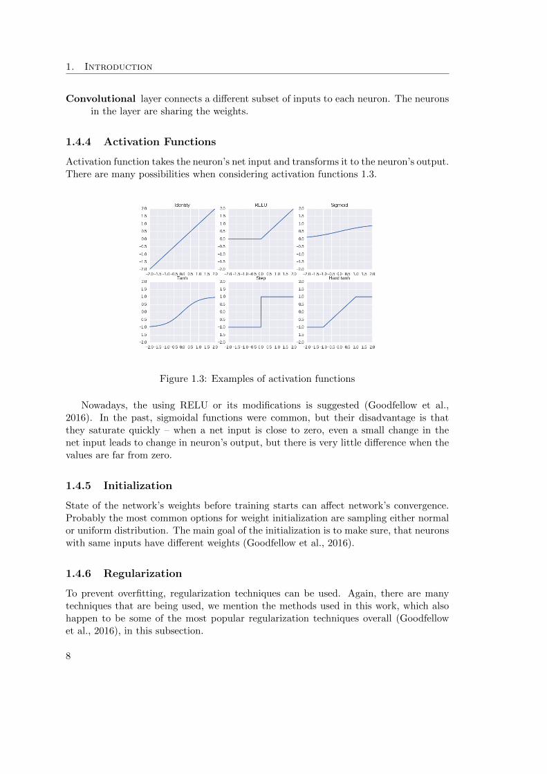
Activation function takes the neuron’s net input and transforms it to the neuron’s output.There are many possibilities when considering activation functions 1.3.

Figure 1.3: Examples of activation functions

Nowadays, the using RELU or its modifications is suggested (Goodfellow et al.,2016). In the past, sigmoidal functions were common, but their disadvantage is thatthey saturate quickly – when a net input is close to zero, even a small change in thenet input leads to change in neuron’s output, but there is very little difference when thevalues are far from zero.

1.4.5 Initialization

State of the network’s weights before training starts can affect network’s convergence.Probably the most common options for weight initialization are sampling either normalor uniform distribution. The main goal of the initialization is to make sure, that neuronswith same inputs have different weights (Goodfellow et al., 2016).

1.4.6 Regularization

To prevent overfitting, regularization techniques can be used. Again, there are manytechniques that are being used, we mention the methods used in this work, which alsohappen to be some of the most popular regularization techniques overall (Goodfellowet al., 2016), in this subsection.

8

1.4. Predictive Modeling

1.4.6.1 Dropout

Dropout removes, with some given probability, a node together with its connectionsfrom the network. By removal of the neurons, sub-networks emerge. The sub-networksare trained in the same way as the whole network. This prevents co-adaptation ofthe neurons. Testing is done on the whole network with all neurons. Such networkapproximates averaging all the sub-networks as an ensemble model. This technique wasintroduced in Srivastava et al., 2014.

1.4.6.2 L1 and L2 Regularization

Another way how to regularize the network is to constrain the weights by adding apenalty to a loss function for weight far from the origin. The penalty is α||w||1 for L1regularization and α1

2 ||w||22 when using L2 regularization.

1.4.7 Early Stopping

Early stopping can be looked upon as a regularization method. The point of earlystopping is to separate part of training data into validation set and monitor (validation)loss during training. When the validation loss stops decreasing for some number ofepochs, the training stops, and the model’s weights are set to the state they were inwhen the validation loss was lowest.

9

Chapter 2

Literature Review

2.1 Betting Markets

In his work Levitt, 2004, the author explained the differences between financial andbetting markets. To examine the markets’ behavior, he used a dataset consisting of 20000 wagers placed on NFL from 285 bettors. While the author had a line from onlyone bookmaker, he argued, that different bookmakers have similar lines probably due tooutsourcing the odds from few odds setters.

Lots of authors interest had been devoted to determining how the odds are set.Two different scenarios in which bookmakers are making money were considered – onebeing bookmakers’ capability of balancing weighted wages, second relying on bookmakersconsistently outperforming gamblers in predictions.

The first hypothesis was quickly rejected by proving that in median game two-thirdsof wages fall to one side. The author provided two feasible explanations. Either it isnot possible for the bookmaker to balance the money wagered or it is not his objective.This rejection implies, that if there was a large enough subset of bettors outperformingthe bookmaker, it would lead to the ruin of the bookmaker.

The author concluded that bookmakers are better in forecasting outcomes of gamesthan an average bettor, which leads to higher profits than relying solely on balancingwages and winning thanks to the margin. While this strategy makes the bookmakervulnerable against more skilled bettor than himself, the bookmaker protects himself bylimiting the distortion of the odds.

The ability to hire experts that are better in forecasting game outcomes than therest of the market was marked as the fundamental difference between betting marketsand financial markets, where such solution is not possible, due to the complexity of themarket and the amount of inside information.

Another interesting question answered was whether the aggregation of the bettors’beliefs carries any useful information. Data suggested that there is a correlation betweenthe percentage of bettors choices and the game outcome such that the results chosen bythe majority of bettors are more likely to happen. However, the author pointed out that

11

2. Literature Review

obtaining information about how the bettors acted before the game is problematic.Rodney J Paul; Andrew P. Weinbach, 2007 raised their concerns about the generality

of Levitt, 2004 findings. They pointed out that Levitt’s dataset consisted of bets frombetting tournament with entry fee and a limited number of participants, therefore notbeing representative. To test the Levitt’s hypothesis, authors gathered percentage betson opposing teams after each match day. Their findings were inline with the Levitt’shypothesis. Much more money was accepted on favorites, which led to the point spreadnot reflecting the market clearing price. They extended the reasons for why is not thebookmakers’ strategy exploitable, stated in Levitt, 2004, with the point, that bettingmarkets are in fact not free and betting sites can limit placed wagers or even refuse thewagers.

Same authors, such as Rodney J. Paul et al., 2008, decided to test the hypothesis onanother sport – basketball. Contrary to observations from NFL, betting against publicbelief did not lead to profit. This lead to the idea, that bookmakers do not always tryto exploit bettors biases, but rather focus on profiting on commissions in the long-run.This strategy wouldn’t create chances for informed bettors. As the reason for followingthis policy authors mentioned smaller market for NBA betting.

Again, the same authors in Rodney J Paul; Andrew P Weinbach, 2010 explored thebehavior of bettors on data from NBA and NHL season 2008/09. The key questionasked was whether a typical bettor is a fan or an investor. The argument was that ifthe bettors are investors, it should be difficult to spot patterns affecting numbers of betsplaced on different games. On the other hand, if the bettors are fans, they are expectedto bet higher volumes on the most attractive games – games with television coverage,uncertain outcome, etc.

Data confirmed the hypothesis, that the bettors’ behavior mimic fans’ behavior tothe point, that authors mention betting as a complement of watching sports events.Authors admit, that small group of bettors acting as investors might still exist; they arehowever the minority.

This finding follows our intuition and it is particularly interesting with the conclusionfrom Levitt, 2004 that the bookmaker focuses on beating the average bettor. Havingconfirmed that an average bettor is a fan, one might hope that with a statistical modelingapproach, without any emotional attachments, it might be possible to exploit this facttowards a profit.

2.2 Human vs Machine

The idea that a statistical model might outperform experts was first tested in Simmonset al., 2000. The experts’ predictions were obtained from three major magazines, andthree different levels of experts’ insights were tested.

• Are they outperforming a random choice?

• Do they efficiently process publicly available data?

• Do they make use of inside information?

12

2.2. Human vs Machine

The prediction accuracy of the experts was about 42 %. In the sample, 47 % of gameswere won by a home team. The authors thought of this comparison as unfair becausethe experts are obliged by the magazines to diversify their predictions. Moreover, whenauthors conducted regression analysis of the statistics in the respective magazines, theexperts were found unable to process publicly available information efficiently. Onlyone of the experts showed signs of using information independent of publicly availabledata. Therefore the authors concluded that there is no reason why the experts shouldoutperform the regression model.

Forrest et al., 2005 challenged the idea, introduced in Simmons et al., 2000, thata statistical model has an edge in comparison with tipsters. They examined the per-formance of a statistical model and bookmakers on 10 000 soccer matches. The authorsconcluded that under financial pressure, the bookmakers are on par with the statist-ical model. They also noticed, that bookmakers’ accuracy improved through the 5-yearperiod. Odds set by the bookmaker were suggested as a useful feature for the statisticalmodel.

Song et al., 2007 analyzed prediction accuracy of experts, statistical models andopening betting lines on two NFL seasons. There was a little difference between statist-ical models and experts performance, but both were outperformed by betting line. Theyeven stated that betting lines are capable of predicting the margin of victory extremelywell.

Authors stated several reasons why they think the experts performed as well as stat-istical models in their setup. First of all, the experts published their predictions in pop-ular national magazines and were responsible for the magazines’ creditability. Moreover,their predictions were posted close to the match day, so they could had accounted forall the information gathered or even make use of inside information since a lot of themwere active players in the past and had connections to the coaches.

As a major advantage of statistical models over the experts, the authors pointed outlower variance between the models – worst models performed much better than worstexperts.

Spann et al., 2009 compared prediction accuracy of prediction markets, betting oddsand tipsters on three seasons of German premier soccer league. The authors tested theprofitability of forecasting methods by betting the same amount of money on all theopportunities that are identified as profitable by the selected method.

Prediction markets and betting odds proved to be comparable in terms of predictionaccuracy. The forecasts from prediction markets would be able to generate profit againstthe betting odds if it wasn’t for the high fees. On the other hand, tipsters performedrather poorly in this comparison.

The fees make it harder to interpret the results since it is not clear if they serve as atool for a bookmaker to increase his edge over the bettors, while offering more fair oddsat first glance, or they are enforced by law as a form of tax.

Authors also examined a weighting-based and a rule-based combination of the fore-casts looking for improvements in accuracy and profitability.

The weighting-based system relied on averaging the predictions made by prediction

13

2. Literature Review

market and bookmaker’s odds. Neither the prediction accuracy nor the profits differedsignificantly from the standalone methods.

A rule-based system was based on a consensus of the forecasting methods. Theprediction accuracy was highest when all the methods agreed. This situation, however,occurred only in about half of the games in the sample. On the contrary, the bettingodds were in agreement with prediction markets in more than 90 % of the games whichled to more betting opportunities and higher profits in total.

Franck; Verbeek; Nuesch, 2010, inspired by results of prediction markets in differentdomains such as politics, compared performance of betting exchange against bookmakeron 3 seasons of 5 European soccer leagues.

Prediction market was superior to the bookmaker in terms of prediction accuracy. Asone of the reasons for this result, authors stated the bookmaker’s intention to maximizethe profit mentioned for example in Levitt, 2004. A simple strategy based on betting onthe opportunities where the average odds set by the bookmakers were higher than oddsin prediction market was profitable in some cases. Especially when predicting a win forthe visiting team, the betting strategy was profitable against all bookmakers but one.

The authors also examined correlations between bookmakers’ odds and predictionmarket. The data showed that the bookmaker and prediction market are highly correl-ated. Both the bookmakers and the prediction market underestimated the number ofoccurrences of home wins.

Kain et al., 2014 challenged the idea that betting markets are accurate predictors.For this purpose, they investigated betting markets performance not only on actualresults of the games but also on under/over bets. Their dataset consisted of bettinglines and under/over odds from NFL, NBA and NCAA seasons 2004-2010.

The authors found out that while betting line performs well when it comes to pre-dicting the outcome of the game, the line for under/over fails to predict the number ofpoints scored in the match.

2.3 Predictive Models

Besides the question, if a statistical model can outperform the human, lot of work havebeen dedicated to predictive modeling, not concerning comparison with the bettingmarket. First of all, we mention two overviews, where a broader spectrum of researchis described. We focus mainly on predictive models applied on basketball. However,interesting approaches tried in other domains are also mentioned.

2.3.1 Overview

Stekler et al., 2010 focused on several topics in horse racing and team sports. Forecastswere divided into three groups by their origin – market, models, experts.

Authors shared several findings that were backed by research in different sports.Closing odds proved to be better predictors of the game outcome than opening odds.Bettors belief in “hot hand” was pointed out – the bettors believe, that after a winning

14

2.3. Predictive Models

game, the probability of the team to win the next game is higher, despite the fact, thatthere is no evidence of dependence.

As the most important result author stated that there was ho evidence that statisticalmodel or expert could consistently outperform betting market.

Haghighat et al., 2013 provided a review of machine learning techniques used inoutcome predictions of sports events. Authors more closely examined 9 papers frompast decade. Common findings were that either presented results are rather poor or theused datasets are too small. For improving the prediction accuracy, it was suggestedto include player-level statistics and machine learning techniques with good results indifferent fields.

2.3.2 Basketball

Loeffelholz et al., 2009 achieved a remarkably high accuracy of over 74% using neuralnetworks, sadly it was on a dataset consisting of only 620 games. As features for theirmodel, the authors used seasonal averages of 11 basic box score statistics for each team.They also tried to use average statistics of past 5 games and averages from home andaway games separately but reported no benefits.

Ivankovic et al., 2010 used ANNs to predict outcomes of basketball games in theLeague of Serbia in seasons 2005/06–2009/10. The most interesting part of the workwas using effects of shots from different court areas as features. With this approach,the authors achieved accuracy of 81 %. However, the very specific dataset makes itimpossible to compare the results with other research.

Miljkovic et al., 2010 evaluated their model on NBA season 2009/10. Basic box scorestatistics were used as features, as well as win percentages in league/conference/divisionand in home/away games. Naive Bayes in 10-fold cross-validation achieved mean accur-acy of 67 %.

Puranmalka, 2013 used play-by-play data (Section 1.3.2) do develop new features.The main reason why features derived from play-by-play data are superior to box scorestatistics is that they include a context. The features were divided into 4 groups asfollows.

The first group contained features already mentioned in the literature. The authordiscussed a so called “clutch performance”. The idea behind measuring clutch perform-ance is to put emphasis on plays made in close matches. Determining which game wasclose based on the final score was criticized. The underlying reasoning was that evenuneven games can end with a relatively low difference in points scored and on the otherhand really close games can end up looking uneven because of teams taking higher risksin the final quarter. A method based on point difference at selected times of last quarterwas proposed. Also measuring shot selection and efficiency was analyzed. The authorexplained that traditional features as points scored/allowed per possession fail to explainwhy is the offense/defense more or less efficient. Instead, expected points per possessionwere suggested. Expected points per possession are based on different types of shotshaving different success rates and occurring with different frequencies.

15

2. Literature Review

The second set of features focused on the distribution of time on the court for playersof each team. Hypothesis, that in the ideal scenario, only five players for each team haveto play each game is stated. Deviation from this scenario is presented as one feature,however, the author acknowledged that deviation might only signalize, that team hasa strong bench. Another feature was proposed based on the variance of players timeon the court between games with the idea, that if the player spends on court similaramount of time each game, his role in team is well defined and the team is effective.

The third group of features tried to catch player-to-player dependencies. The authorquestioned predictive models for assuming that players’ performances are independentof each other. Instead, he focused on pairs of players and how their offensive efficiencychanges, when they are playing together. To measure defensive efficiency author ex-amined how offensive efficiency of opposing team changes while the player is on thecourt.

The fourth set of features captured team-to-team interactions, like what happenswhen teams strong in certain ways (rebounds, fouls drawn, etc.) plays a team weak inthat way. Several statistics were measured and teams ranked in each category. Relev-ant ranking pairs (for example strong team in the category playing weak team in thecategory) were marked as the new feature.

The last group of features was considered the most important one – context addedmetrics. The author found out, that there is a strong correlation between points perpossession and time left on shot clock. The new feature was derived from time left onshot clock, attacking team’s offensive efficiency and defending team’s defensive efficiency.

A genetic algorithm for feature selection was compared with forward selection. For-ward selection proved to be more effective. In the model using team-level features,clutch performance defined by author proved to be one of the best predictors of gameoutcome. Also, team-to-team features turned out to be very valuable. In player-levelmodel, the context added metrics were the most useful. On the contrary, classic featureslike distance traveled or number of rest days between matches didn’t seem to have anypredicting power.

Out of Naive Bayes, Logistic Regression, Bayes Net, SVM and k-nn, the SVM per-formed best, achieving accuracy over 71 % in course of 10 NBA season from 2003/04 to2012/13.

Even though we decided not to make use of play-by-play data, we consider this workvery relevant and novel. It could serve either as possible extension of our models or forcomparison of models’ performance.

Zimmermann et al., 2013 leveraged multi-layer perceptrons, that hadn’t been usuallyused in this domain. They also raised their concern, that there might be a glass ceilingof about 75 % accuracy based on results achieved by statistical models in numerousdifferent sports. This glass ceiling could be caused by using similar features in manypapers. They also argued that features are much more important than machine learningmodels since even Naive Bayes performed well. To increase the predictive power of theirmodels, features encoding experience and leadership were used. An interesting ideamentioned in the paper is to train separate model for intra-conference matches.

16

2.4. Features

Yang, 2015 analyzed the relation between player statistics and its team’s performancein past 20 seasons of NBA. To regress player statistics to team strength, player efficiencyrating was used. Team strength (team PER) was calculated as a weighted sum of players’PER. Point was made, that basketball is flooded with overcomplicated statistics whilewe can use basic stats to estimate the strength of a player or a team.

Vracar et al., 2016 made use of play-by-play data to simulate basketball games asMarkov processes. Analysis of the results showed that a basketball game is a homogen-eous process excluding very beginning and end of each quarter. Modeling these sequencesof the game had a large impact on forecast performance. The author saw the applicationof their model not only in outcome prediction before the game but also in in-play bettingon less common bets (number of rebounds/fouls in specific period of the game).

2.3.3 Other

Basketball is by no means the only sport, where various forecasting models were tested.Here we briefly mention several interesting approaches tested in other sports.

Hvattum et al., 2010 implemented ELO rating (the standard way of determiningchess players’ strength) to express soccer teams’ strength. ELO rating method performedpoorly in comparison with methods based on betting odds.

Constantinou et al., 2013 designed an ensemble of Bayesian networks to asses soccerteams’ strength. Besides objective information, they accounted for the subjective typeof information such as team form, psychological impact, and fatigue. All three compon-ents showed a positive contribution to models’ forecasting capabilities. Including fatiguecomponent provided the highest performance boost. Results revealed conflicts betweenaccuracy and profit measures. The author emphasized the importance of expert know-ledge when it comes to subjective inputs. The final model was able to outperform thebookmakers. The article demonstrates predictive power of Bayesian networks when welldesigned. However since we do not posses domain knowledge needed to properly designsuch a network, we decided to stay away from this model.

Sinha et al., 2013 made use of twitter posts to predict the outcomes of NFL games.Information from twitter posts enhanced forecasting accuracy, moreover, model basedsolely on features extracted from tweets outperformed models based on traditional stat-istics.

2.4 Features

During the game of basketball, a variety of statistics is being recorded. Getting an insightinto these statistics could be crucial for feature selection or later model interpretability.We conducted research in order to close the gap in our game knowledge.

Kubatko et al., 2007 had set a starting point for analyzing basketball statistics. Theconcept of equal possessions for opposing teams was defined as key to basketball analysis.Formulas for estimating possessions were reviewed. Statistics from non-academic sourceswere brought together and explained.

17

2. Literature Review

Sergio J. Ibanez et al., 2008 tried to identify statistics that differentiate the successfulteams from the less successful ones. All statistics were normalized according to ballpossessions as was suggested in Kubatko et al., 2007. The most discriminative statisticsfound were assists, steals, and blocks. The classification function was correct in 82.4 %retrospectively. Another result was that pace of the games is not an indicator of theteam’s performance.

Sergio J Ibanez et al., 2009 focused on variations in game-related statistics makingthe difference in winning and losing in three consecutive games. Authors concluded thatthere was no significant variance in team performance. High fitness levels of players andthe unlimited number of substitutions were stated as possible causes of this outcome.

Sampaio et al., 2010 studied effects of season period, team quality on players’ statist-ics. Their dataset consisted of more than 5000 records from nearly 200 players in Spanishprofessional basketball league season 2007-08. Weaker teams showed larger discrepanciesbetween their strongest and weakest players performances. Players that spend less timeon the court tend to do more errors. Authors found no variation in players’ performanceduring the season. This result is crucial for our work, because it implies, that once weobtain the team strength, we do not need to worry about its variation in time.

Strumbelj, 2014 addressed two very important questions. First one was whether itmakes a difference which bookmaker we choose and a second one concerning derivingprobabilities from betting odds. To answer these questions, the authors gathered adataset consisting of almost 50000 games from numerous team sports. In literature,underlying probabilities are usually calculated by dividing inverse odds by their sum.This work, however, showed that using model form Shin, 1991 we can obtain moreaccurate predictions. Betting exchange Betfair and betting sites bet365 and bwin provedto be most accurate on average. On the other hand bookmaker Interwetten was pointedout as the worst source of probability forecasts. Moreover, it performed particularlypoor in basketball.

18

Chapter 3

Analysis and Design

In order to build a system that we could test against a betting market, several stepshad to be done. Firstly, we had to gather and process as much relevant data as possiblefrom a variety of sources and decide on how to build datasets from this raw data. Afterthat came the statistical analysis and machine learning part. These, however, were notthe final step of our work, since to evaluate the learned model against odds set by thebookmaker, a betting strategy also had to be determined. Each step of this pipeline isdescribed in the following sections.

3.1 Gathering Data

Collecting data proved to be a challenging task. There are no widely recognized datasets.Plenty of data is available online, however, it is not for free.

Obtaining historical betting odds is an even bigger problem. The betting sites donot provide such data. There are websites specializing in collecting the odds from avariety of bookmakers. It is not usually stated whether the presented odds are openingor closing odds set by the bookmaker. Sometimes these websites show the best oddsavailable among the bookmakers for each outcome of a game. To make practical useof such information, one would have to set an account on every betting site listed anddeposit money to all these accounts.

In the end, we managed to gather official box score data 1.3.2 from NBA seasons2000 to 2014. As for betting odds, we used Pinnacle closing odds for seasons 2010-2014,provided by Assistant Professor Strumbelj. For previous seasons we gathered odds fromdifferent bookmakers.

3.2 Building Datasets

After the data were stored into a relational database, they had to be preprocessed andaggregated into the datasets.

19

3. Analysis and Design

The basic premise for meaningful forecasting is to use only the data obtained beforethe forecast could be done. In our case, that means using the data available before thestart of the game. Box scores are statistics gathered during the game so they cannotbe used for forecasting by themselves. On the other hand betting odds are known daysbefore the game actually starts so they could be included as features. We discussed twoapproaches how to extract features from the database.

3.2.1 Teams’ and Players’ Seasonal Averages

Seasonal averages are widely used in literature. They serve as a good predictor of teamstrength. However, beginnings of the seasons are problematic because the averageschange rapidly. We experimented with excluding a different number of games fromseason beginning from training and testing our model. The downside of this approachis that the system cannot bet in these first rounds before seasonal averages settle.

3.2.2 Teams’ and Players’ Last n Games

Most of the research focused on in-game momentum (see Bar-Eli et al., 2006 for review),analyzing for example if series of successful shots increase the probability that the nextshot taken will also be successful. However, some research has also been done on seasonscale – if a streak of won games increases the probability that the team will win the nextone. Vergin, 2000, Goddard et al., 2004 and Sire et al., 2009 found no evidence for suchmomentum while more recent work Arkes et al., 2011 claims opposite. We decided notto use the last n games of opposing teams for dataset creation, although it might be asubject of our future work.

3.3 Exploratory Data Analysis of Bookmakers’ Odds

Among all the features, one type is particularly interesting - the bookmaker’s odds.Bookmaker’s odds can be used as an input to our model, but at the same time, themodel will be evaluated using ground truth labels together with these odds througha selected betting strategy. In this section, we analyze odds set by the bookmakerto discover possible biases which could create opportunities for exploitation. Unlessspecified otherwise, data we are analyzing are closing odds from “Pinnacle” on gameoutcomes from seasons 2010/11–2014/15.

3.3.1 Odds Distribution

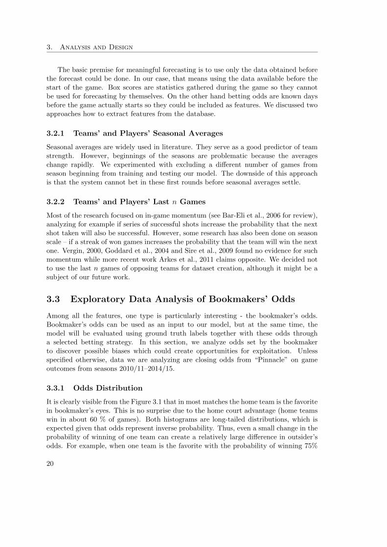
It is clearly visible from the Figure 3.1 that in most matches the home team is the favoritein bookmaker’s eyes. This is no surprise due to the home court advantage (home teamswin in about 60 % of games). Both histograms are long-tailed distributions, which isexpected given that odds represent inverse probability. Thus, even a small change in theprobability of winning of one team can create a relatively large difference in outsider’sodds. For example, when one team is the favorite with the probability of winning 75%

20

3.3. Exploratory Data Analysis of Bookmakers’ Odds

Figure 3.1: Distribution of odds set by the bookmaker for home team (left) and forvisiting team (right).

and another team is also favorite, but with probability 76%, fair odds would be 1.33 and1.32 respectively. Fair odds for their opponents would be 4 and 4.17.

3.3.2 Margin Analysis

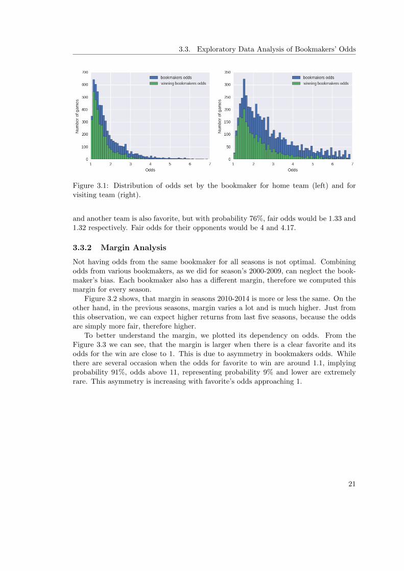
Not having odds from the same bookmaker for all seasons is not optimal. Combiningodds from various bookmakers, as we did for season’s 2000-2009, can neglect the book-maker’s bias. Each bookmaker also has a different margin, therefore we computed thismargin for every season.

Figure 3.2 shows, that margin in seasons 2010-2014 is more or less the same. On theother hand, in the previous seasons, margin varies a lot and is much higher. Just fromthis observation, we can expect higher returns from last five seasons, because the oddsare simply more fair, therefore higher.

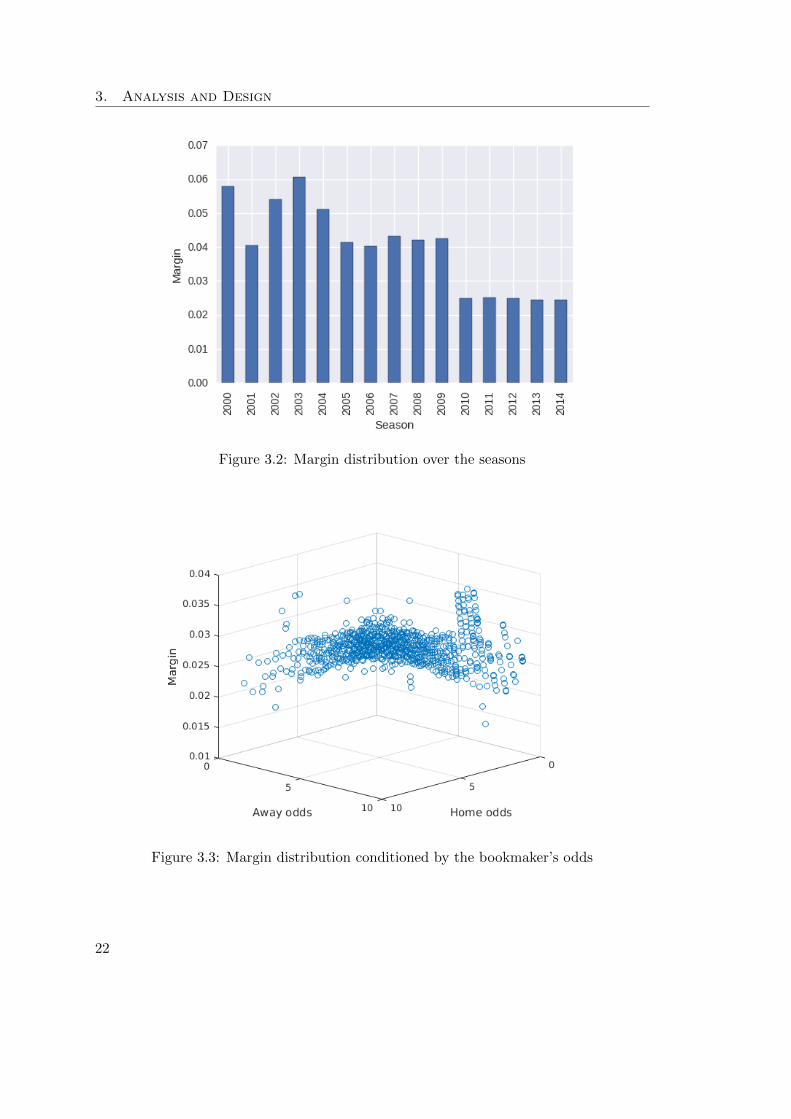
To better understand the margin, we plotted its dependency on odds. From theFigure 3.3 we can see, that the margin is larger when there is a clear favorite and itsodds for the win are close to 1. This is due to asymmetry in bookmakers odds. Whilethere are several occasion when the odds for favorite to win are around 1.1, implyingprobability 91%, odds above 11, representing probability 9% and lower are extremelyrare. This asymmetry is increasing with favorite’s odds approaching 1.

21

3. Analysis and Design

Figure 3.2: Margin distribution over the seasons

Figure 3.3: Margin distribution conditioned by the bookmaker’s odds

22

3.4. Predictive Modeling

3.4 Predictive Modeling

3.4.1 Estimates Based on Bookmaker’s Odds

We used the gathered data to estimate the distribution of P (RESULT |ODDS,COURT )with the assumption that this trivial model might reveal some systematic biases andprovide useful information for our model.

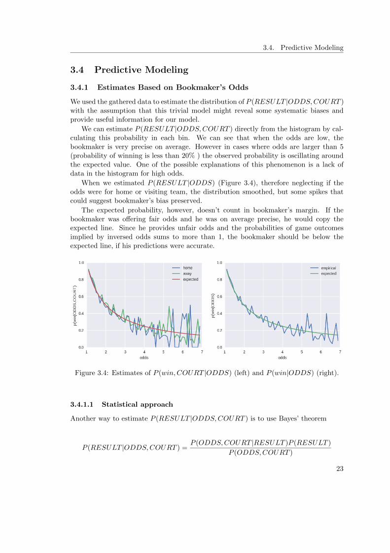
We can estimate P (RESULT |ODDS,COURT ) directly from the histogram by cal-culating this probability in each bin. We can see that when the odds are low, thebookmaker is very precise on average. However in cases where odds are larger than 5(probability of winning is less than 20% ) the observed probability is oscillating aroundthe expected value. One of the possible explanations of this phenomenon is a lack ofdata in the histogram for high odds.

When we estimated P (RESULT |ODDS) (Figure 3.4), therefore neglecting if theodds were for home or visiting team, the distribution smoothed, but some spikes thatcould suggest bookmaker’s bias preserved.

The expected probability, however, doesn’t count in bookmaker’s margin. If thebookmaker was offering fair odds and he was on average precise, he would copy theexpected line. Since he provides unfair odds and the probabilities of game outcomesimplied by inversed odds sums to more than 1, the bookmaker should be below theexpected line, if his predictions were accurate.

Figure 3.4: Estimates of P (win,COURT |ODDS) (left) and P (win|ODDS) (right).

3.4.1.1 Statistical approach

Another way to estimate P (RESULT |ODDS,COURT ) is to use Bayes’ theorem

P (RESULT |ODDS,COURT ) =P (ODDS,COURT |RESULT )P (RESULT )

P (ODDS,COURT )

23

3. Analysis and Design

To make a use of the formula, an assumption about P (ODDS,COURT ) andP (ODDS,COURT |RESULT ) distributions has to be made. The Beta distribution isthe conjugate prior distribution for Bernoulli distribution, so it fits our case nicely. Eachgame can be looked upon as a Bernoulli trial. The team has a certain probability p ofwinning the game. The value of p is the only parameter needed for defining the Bernoullidistribution. This probability p also comes from a distribution – the distribution ofprobabilities. Beta distribution is defined in the interval [0, 1], therefore it can be usedas the distribution over probability.

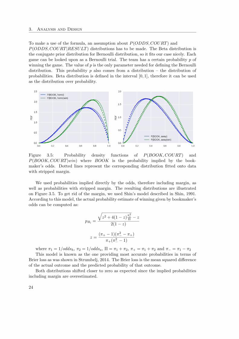
Figure 3.5: Probability density functions of P (BOOK,COURT ) andP (BOOK,COURT |win) where BOOK is the probability implied by the book-maker’s odds. Dotted lines represent the corresponding distribution fitted onto datawith stripped margin.

We used probabilities implied directly by the odds, therefore including margin, aswell as probabilities with stripped margin. The resulting distributions are illustratedon Figure 3.5. To get rid of the margin, we used Shin’s model described in Shin, 1991.According to this model, the actual probability estimate of winning given by bookmaker’sodds can be computed as:

pBi =

√z2 + 4(1− z)π

2i

Π − z2(1− z)

z =(π+ − 1)(π2

− − π+)

π+(π2− − 1)

where π1 = 1/oddsh, π2 = 1/oddsa, Π = π1 + π2, π+ = π1 + π2 and π− = π1 − π2

This model is known as the one providing most accurate probabilities in terms ofBrier loss as was shown in Strumbelj, 2014. The Brier loss is the mean squared differenceof the actual outcome and the predicted probability of that outcome.

Both distributions shifted closer to zero as expected since the implied probabilitiesincluding margin are overestimated.

24

3.4. Predictive Modeling

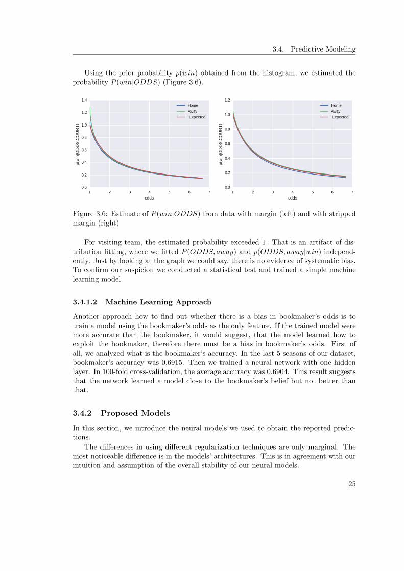
Using the prior probability p(win) obtained from the histogram, we estimated theprobability P (win|ODDS) (Figure 3.6).

Figure 3.6: Estimate of P (win|ODDS) from data with margin (left) and with strippedmargin (right)

For visiting team, the estimated probability exceeded 1. That is an artifact of dis-tribution fitting, where we fitted P (ODDS, away) and p(ODDS, away|win) independ-ently. Just by looking at the graph we could say, there is no evidence of systematic bias.To confirm our suspicion we conducted a statistical test and trained a simple machinelearning model.

3.4.1.2 Machine Learning Approach

Another approach how to find out whether there is a bias in bookmaker’s odds is totrain a model using the bookmaker’s odds as the only feature. If the trained model weremore accurate than the bookmaker, it would suggest, that the model learned how toexploit the bookmaker, therefore there must be a bias in bookmaker’s odds. First ofall, we analyzed what is the bookmaker’s accuracy. In the last 5 seasons of our dataset,bookmaker’s accuracy was 0.6915. Then we trained a neural network with one hiddenlayer. In 100-fold cross-validation, the average accuracy was 0.6904. This result suggeststhat the network learned a model close to the bookmaker’s belief but not better thanthat.

3.4.2 Proposed Models

In this section, we introduce the neural models we used to obtain the reported predic-tions.

The differences in using different regularization techniques are only marginal. Themost noticeable difference is in the models’ architectures. This is in agreement with ourintuition and assumption of the overall stability of our neural models.

25

3. Analysis and Design

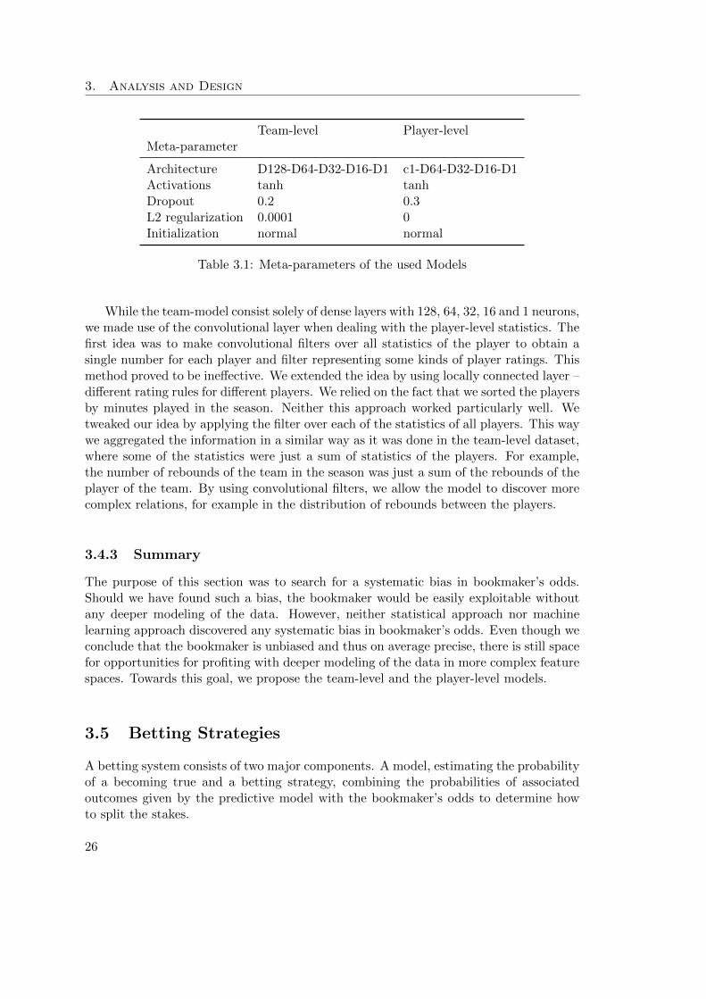
Team-level Player-levelMeta-parameter

Architecture D128-D64-D32-D16-D1 c1-D64-D32-D16-D1Activations tanh tanhDropout 0.2 0.3L2 regularization 0.0001 0Initialization normal normal

Table 3.1: Meta-parameters of the used Models

While the team-model consist solely of dense layers with 128, 64, 32, 16 and 1 neurons,we made use of the convolutional layer when dealing with the player-level statistics. Thefirst idea was to make convolutional filters over all statistics of the player to obtain asingle number for each player and filter representing some kinds of player ratings. Thismethod proved to be ineffective. We extended the idea by using locally connected layer –different rating rules for different players. We relied on the fact that we sorted the playersby minutes played in the season. Neither this approach worked particularly well. Wetweaked our idea by applying the filter over each of the statistics of all players. This waywe aggregated the information in a similar way as it was done in the team-level dataset,where some of the statistics were just a sum of statistics of the players. For example,the number of rebounds of the team in the season was just a sum of the rebounds of theplayer of the team. By using convolutional filters, we allow the model to discover morecomplex relations, for example in the distribution of rebounds between the players.

3.4.3 Summary

The purpose of this section was to search for a systematic bias in bookmaker’s odds.Should we have found such a bias, the bookmaker would be easily exploitable withoutany deeper modeling of the data. However, neither statistical approach nor machinelearning approach discovered any systematic bias in bookmaker’s odds. Even though weconclude that the bookmaker is unbiased and thus on average precise, there is still spacefor opportunities for profiting with deeper modeling of the data in more complex featurespaces. Towards this goal, we propose the team-level and the player-level models.

3.5 Betting Strategies

A betting system consists of two major components. A model, estimating the probabilityof a becoming true and a betting strategy, combining the probabilities of associatedoutcomes given by the predictive model with the bookmaker’s odds to determine howto split the stakes.

26

3.5. Betting Strategies

3.5.1 Motivation

From the odds we can derive probability of winning estimated by bookmaker pB. Outputof our prediction model is another estimation pM of the true probability pT . There aredifferent scenarios that can occur as follows.

pM < pB < pT (3.1)

pM < pT < pB (3.2)

pB < pM < pT (3.3)

pB < pT < pM (3.4)

pT < pM < pB (3.5)

pT < pB < pM (3.6)

When pB < pT , the bookmaker underestimated the likelihood of the event and set theodds too high, creating an opportunity for generating profit. On the other hand, whenpB > pT , then the set odds are skewed in bookmaker’s favor.

When pB < pM we assume, that bookmaker had set the odds too high, thereforewe bet, otherwise we don’t. However, how much we bet depends on a chosen bettingstrategy.

3.5.2 Definition

We can define the betting strategy for n betting opportunities as a following:

f : Mn ×Bn →Wn

Mi = probability of winning given by model

Bi = probability of winning given by bookmaker’s odds

Wi = portion of wealth staked

For each round of league matches consisting of n2 matches the bookmaker sets odds for

each outcome, creating n betting opportunities. Our model output its own estimates ofthe probabilities. A betting strategy takes the bookmakers odds and the model’s estim-ates and outputs portion of wealth (the bets) to be waged on each betting opportunity.

3.5.3 Expected Return and Variance of Profit of a Bet

For each betting opportunity oppi we can calculate the expected return and the varianceas

E(oppi) = pwini(oddsi − 1) + (1− pwini)(−1) = pwinioddsi − 1 (3.7)

σ2 = E[X2]− E[X]2 = pwini(1− pwini)odds2i (3.8)

27

3. Analysis and Design

where pwini is the estimated probability of the opportunity coming true and oddsi areodds set by the bookmaker.

The true probability of betting opportunity coming true is unknown. Therefore weuse our model’s estimate to calculate the expected profit instead.

3.5.4 Betting Strategies in Literature

In the literature, we have encountered several betting strategies as follows.

• Bet fixed amount on favorable odds (fixbet).

• Bet amount equal to the absolute discrepancy between probabilities predicted bythe model and the bookmaker (abs disc bet).

• Bet amount equal to the relative discrepancy between probabilities predicted bythe model and the bookmaker (rel disc bet).

• Bet amount equal to the estimated probability of winning (conf bet).

However these strategies have not been formally analyzed in terms of risk, thereforewe question their optimality. Moreover, we can show that according to the laid outcriteria, none of these strategies is optimal.

3.5.5 Betting Strategies by Tipsters

There are plenty of tipsters online, offering their free or paid services. Customer sub-scribes to a service and then before each league round he receives tips on which bettingopportunities are profitable. The tipster usually advises staked amount in terms of units.For each match, there is a possibility to bet 0-10 units. What these units represent inthe model of the tipster is unclear. However, tipsters’ goals are the same - to maximizethe profit and minimize the risk. Moreover, without knowing the tipster’s probabil-ity estimates along with the proposed units staked, determining his betting strategy isimpossible.

3.5.6 Markowitz’s Model

If our goal would be solely to maximize the expected profit, then the solution would betrivial – bet whole wealth on the opportunity with highest expected return of profit frompresented opportunities. However, since the betting is a repeated process, we want somelevel of guarantee that we will have money available for the next betting opportunities.For these reasons, our criteria for selecting the betting strategy are expected profitand risk. Therefore whenever we mention the maximization of the profit, we refer tomaximization of the profit while minimizing the risk.

28

3.5. Betting Strategies

We use a model described in Markowitz, 1952 to find the optimal strategy. TheMarkowitz’s model (also known as Modern Portfolio Theory) is used in economics 1 forportfolio optimization, which is a problem very similar to the one we are facing. Theportfolio assets can be viewed as the betting opportunities at our hand before each ofthe league rounds.

3.5.6.1 Expected Return and Variance of the Portfolio’s Profit

The expected return of the portfolio and the variance are defined as

E(Rp) =∑

wiE(Ri) (3.9)

σ2p =

∑w2i σ

2i +

∑∑wiwjσiσjpij (3.10)

where Rp is the return of the portfolio, σ2p is the variance of the portfolio, wi is the

wealth staked on asset i, Ri is return of asset i, σ2i is the variance of return of asset i

and pij is the correlation of returns of assets i and j.

In our case, we may reasonably assume that outcomes of matches are not correlated,so the variance of the portfolio simplifies to σ2

p =∑w2i σ

2i .

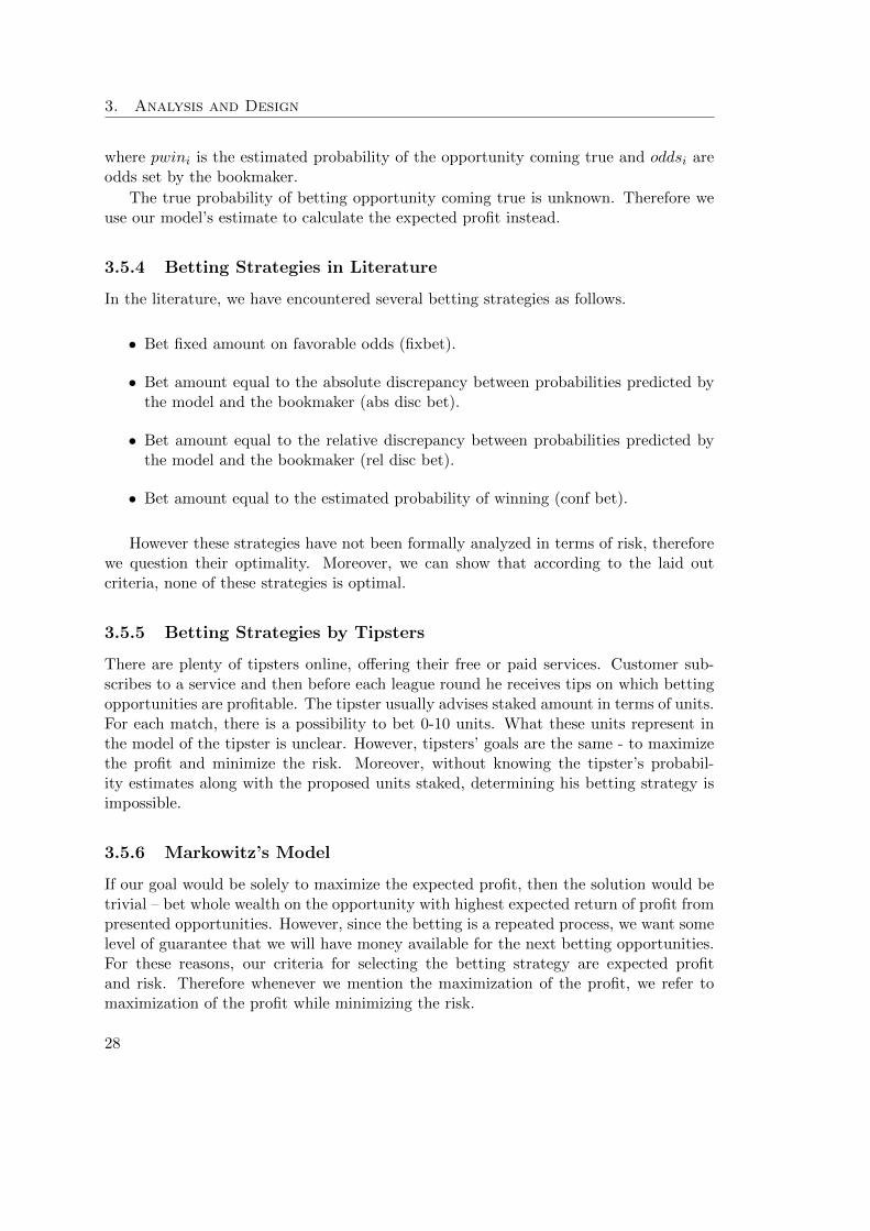
3.5.6.2 Efficient Frontier

Every possible distribution of bets given opportunities can be plotted into a so calledrisk-expected return space. The efficient frontier is then another term for Pareto-frontier.Pareto frontier is a set of solutions to a problem with multiple objectives, where im-proving in one objective would worsen another objective. In our case, such a solution isan allocation of the bets among the betting opportunities such that different allocationwould lead to higher risk or lower expected return.

3.5.6.3 Proposed Strategy

We have decided to choose the final opt strategy from the frontier using Sharpe ratiointroduced in Sharpe, 1994 as

rp − rfσp

where σp is standard deviation of portfolio return, rp is expected return of the port-folio and rf is a risk-free rate. We neglect the risk free rate because there is no risk-freemethod how to appreciate the money during the duration of a match.

The proposed opt strategy is a strategy from the frontier that maximizes the Sharperatio.

1The author was later on awarded Nobel Prize in Economic Sciences.http://www.nobelprize.org/nobel_prizes/economic-sciences/laureates/1990/

29

3. Analysis and Design

Figure 3.7: Risk-expected return space with random strategies and efficient frontier

3.5.6.4 Criticism of Markowitz’s Model

There has been some criticism on Markowitz’s model. Here we take a look at the mainpoints of the criticism.

Risks and returns are based on expected values. These values change intime (they are subjects of volatility). Once the bet is placed there are only twooutcomes possible. Losing the bet or winning bet × odds money. Bets can be placedup to few minutes before the match starts, so the predictive model can accommodatecurrent information, e.g. about team injuries.

Variance is a symmetric measure therefore extremely high returns are asrisky as extremely low returns This downside, unfortunately, prevails in our case,too.

3.5.7 Evaluating Betting Strategies

Now when we introduced the framework we use to evaluate the betting strategies, wecan evaluate the betting strategies we have encountered in the literature in terms of riskand expected profit.

The biggest downfall of the strategies mentioned in Section 3.5.4 is that they operatewith different amount of wealth making them incomparable. To compare these strategieswe had to normalize the bets placed on the betting opportunities so they sum up to 1.

To demonstrate the differences between the betting strategies we randomly sampleddata representing six illustrative betting opportunities with positive expected return

30

3.5. Betting Strategies

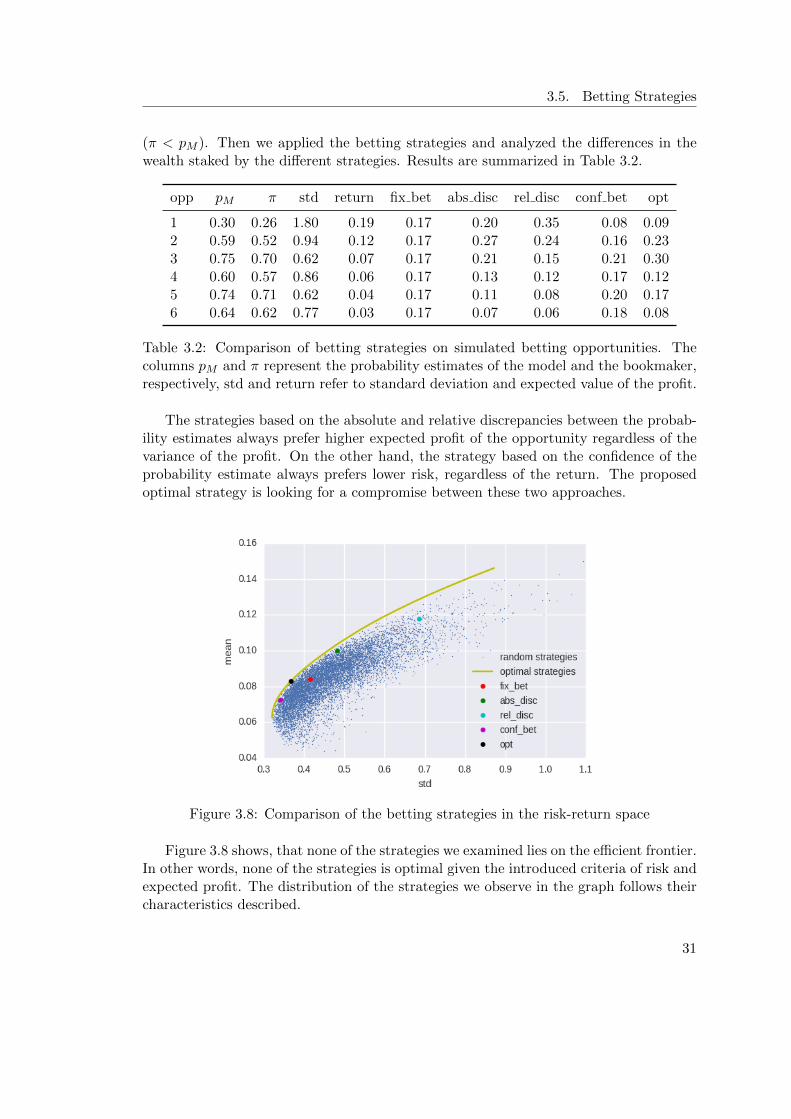
(π < pM ). Then we applied the betting strategies and analyzed the differences in thewealth staked by the different strategies. Results are summarized in Table 3.2.

opp pM π std return fix bet abs disc rel disc conf bet opt

1 0.30 0.26 1.80 0.19 0.17 0.20 0.35 0.08 0.092 0.59 0.52 0.94 0.12 0.17 0.27 0.24 0.16 0.233 0.75 0.70 0.62 0.07 0.17 0.21 0.15 0.21 0.304 0.60 0.57 0.86 0.06 0.17 0.13 0.12 0.17 0.125 0.74 0.71 0.62 0.04 0.17 0.11 0.08 0.20 0.176 0.64 0.62 0.77 0.03 0.17 0.07 0.06 0.18 0.08

Table 3.2: Comparison of betting strategies on simulated betting opportunities. Thecolumns pM and π represent the probability estimates of the model and the bookmaker,respectively, std and return refer to standard deviation and expected value of the profit.

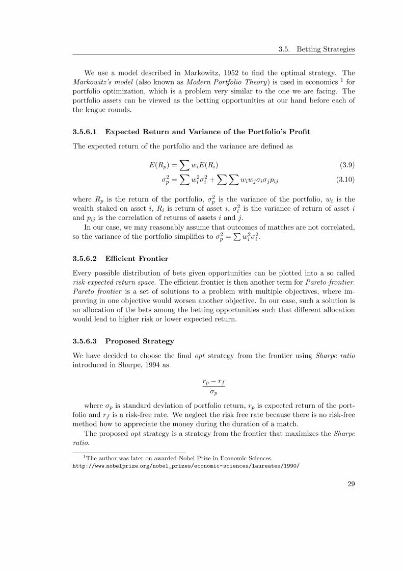
The strategies based on the absolute and relative discrepancies between the probab-ility estimates always prefer higher expected profit of the opportunity regardless of thevariance of the profit. On the other hand, the strategy based on the confidence of theprobability estimate always prefers lower risk, regardless of the return. The proposedoptimal strategy is looking for a compromise between these two approaches.

Figure 3.8: Comparison of the betting strategies in the risk-return space

Figure 3.8 shows, that none of the strategies we examined lies on the efficient frontier.In other words, none of the strategies is optimal given the introduced criteria of risk andexpected profit. The distribution of the strategies we observe in the graph follows theircharacteristics described.

31

Chapter 4

Experiments

4.1 Simulation of the Betting Strategy

To get a better idea of how our selected betting strategy behaves, we generated dataand observed the behavior on them. Generated data consisted of triplets representingthe true probability of winning, the model’s estimate and the bookmaker’s estimate.For a joint analysis of all the hidden factors, the data were generated from a multivari-ate beta distribution parametrized with the means and the variances of the marginaldistributions, representing the ground truth, model’s and bookmaker’s estimates, andtheir mutual correlations. The parameters of this joint distribution were subject totuning and subsequent analysis. However, the marginal distribution representing thebookmaker was fitted with the real historical data obtained from a bookmaker. Sincewe didn’t consider separate cases for home and away games, the mean of the groundtruth model was set to 0.5, however, the variance was in principle unknown. The actualoutcome of a game was determined by a Bernoulli trial.

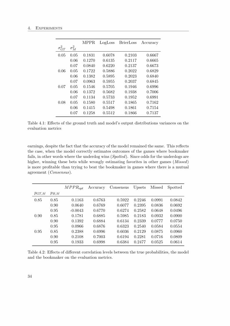
Firstly we examined the effect of our model’s variance on the profit. Table 4.1 shows,that model with lower variance yields higher profit regardless of the variance of theground truth. Other metrics such as Log loss, Brier loss and accuracy are independentof the model’s variance.

We inspected different scenarios that can occur depending on the bookmaker’s pre-diction, our model’s prediction and the actual outcome as follows.

If one team is a favorite in the eyes of the bookmaker, our model agrees, and thisfavorite wins, we call this scenario Consensus. If this team loses, we call it an Upset. Ifour model determined the opposite team as the favorite and was correct in that decision,we say the model Spotted an opportunity. If the model is not right, we conclude it asMissed. When we analyze the models w.r.t. these scenarios, we inspect the portion ofgames in each category.

We examined the relation between the profit and correlation of model’s and book-maker’s estimate, as we expected this to be the core factor in profitability. In agreementwith our intuition, we found out that lower correlation with bookmaker leads to higher

33

4. Experiments

MPPR LogLoss BrierLoss Accuracyσ2GT σ2

M

0.05 0.05 0.1831 0.6078 0.2103 0.66670.06 0.1270 0.6135 0.2117 0.66650.07 0.0840 0.6220 0.2137 0.6673

0.06 0.05 0.1722 0.5886 0.2022 0.68290.06 0.1382 0.5895 0.2023 0.68400.07 0.0963 0.5955 0.2037 0.6845

0.07 0.05 0.1546 0.5705 0.1946 0.69960.06 0.1372 0.5682 0.1938 0.70060.07 0.1134 0.5733 0.1952 0.6991

0.08 0.05 0.1580 0.5517 0.1865 0.71620.06 0.1415 0.5498 0.1861 0.71540.07 0.1258 0.5512 0.1866 0.7137

Table 4.1: Effects of the ground truth and model’s output distributions variances on theevaluation metrics

earnings, despite the fact that the accuracy of the model remained the same. This reflectsthe case, when the model correctly estimates outcomes of the games where bookmakerfails, in other words where the underdog wins (Spotted). Since odds for the underdogs arehigher, winning these bets while wrongly estimating favorites in other games (Missed)is more profitable than trying to beat the bookmaker in games where there is a mutualagreement (Consensus).

MPPRopt Accuracy Consensus Upsets Missed SpottedpGT,M pB,M

0.85 0.85 0.1163 0.6763 0.5922 0.2246 0.0991 0.08420.90 0.0640 0.6769 0.6077 0.2395 0.0836 0.06920.95 -0.0043 0.6770 0.6274 0.2582 0.0648 0.0496

0.90 0.85 0.1781 0.6885 0.5985 0.2183 0.0932 0.09000.90 0.1392 0.6884 0.6134 0.2339 0.0777 0.07500.95 0.0966 0.6876 0.6323 0.2540 0.0584 0.0554

0.95 0.85 0.2388 0.6996 0.6036 0.2129 0.0875 0.09600.90 0.2108 0.7003 0.6194 0.2281 0.0716 0.08090.95 0.1933 0.6998 0.6384 0.2477 0.0525 0.0614

Table 4.2: Effects of different correlation levels between the true probabilities, the modeland the bookmaker on the evaluation metrics.

34

4.2. Model Evaluation

4.2 Model Evaluation

4.2.1 Experiment Setup

In all the experiments, in order to obtain statistically conclusive results, we performedcross-validation as follows. Each season represents one fold in our setup. This way,when a model is tested on, for example, season 2012, the remaining seasons, includingseasons 2013 and 2014, are in the training set. Since the datasets consist of the seasonalaverages, there is no risk of corrupting the results as there is clearly no overlap betweenthe training and test sets. Moreover, no features, that could identify the same team indifferent splits and therefore lead to assumptions about team strength based on matchesthat have yet to be played, are present.

The goal of this work was to exploit the bookmaker, hence we focus primarily onthe profit measure. To measure the profit of the model, we use mean profit per round(MPPR). In NBA, the bookmakers usually set the odds for the next round of leaguematches in advance. After the odds are set, we can deduce the returns with our modeland spread the bets according to our betting strategy. There are 30 teams in NBA, soone league round consists of 15 games. Table 4.3 summarizes the number of games forwhich we predicted the outcomes in each season and the bookmaker’s accuracy in eachseason, respectively. The number of games differs between the seasons because we hadto exclude games with incomplete statistics. Moreover, the first ten games of each teamare not included as they serve for the initial calculation of seasonal averages.

The results presented (f.e. in Table 4.4) are averaged over the validation splits.

4.2.2 Baseline Model

Logistic Regression on team-level dataset served as our baseline model. Logistic Regres-sion is a simple linear model that can be looked upon as ANN with only one neuron usingsigmoid as the activation function. Therefore it serves well as an indicator for structuraland meta-parameter setup of our extended neural models. Moreover, although beinga classifier, it naturally regresses posterior probability of the target classes, and so itsoutput can be directly interpreted as a probability, as required in our subsequent exper-iments with betting strategies.

In the experiments, the baseline model was losing money in the course of 15 seasons.Interestingly, the model’s accuracy was lower than the bookmaker’s even though thebookmaker’s odds were presented in the features.

4.2.3 ANN Model

Our ANN model outperformed baseline model both in the accuracy and the profitability(Table 4.4).

Beating bookmaker in terms of accuracy proved to be a very hard task, even thoughthe bookmaker’s predictions are known to our model. This paradox signalizes, thatdespite the fact that we used several regularization techniques, the model was fitting

35

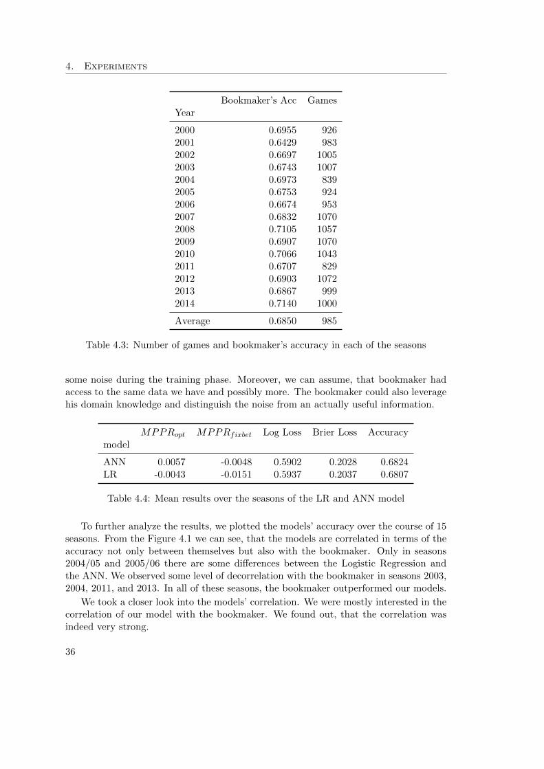
4. Experiments

Bookmaker’s Acc GamesYear

2000 0.6955 9262001 0.6429 9832002 0.6697 10052003 0.6743 10072004 0.6973 8392005 0.6753 9242006 0.6674 9532007 0.6832 10702008 0.7105 10572009 0.6907 10702010 0.7066 10432011 0.6707 8292012 0.6903 10722013 0.6867 9992014 0.7140 1000

Average 0.6850 985

Table 4.3: Number of games and bookmaker’s accuracy in each of the seasons

some noise during the training phase. Moreover, we can assume, that bookmaker hadaccess to the same data we have and possibly more. The bookmaker could also leveragehis domain knowledge and distinguish the noise from an actually useful information.

MPPRopt MPPRfixbet Log Loss Brier Loss Accuracymodel

ANN 0.0057 -0.0048 0.5902 0.2028 0.6824LR -0.0043 -0.0151 0.5937 0.2037 0.6807

Table 4.4: Mean results over the seasons of the LR and ANN model

To further analyze the results, we plotted the models’ accuracy over the course of 15seasons. From the Figure 4.1 we can see, that the models are correlated in terms of theaccuracy not only between themselves but also with the bookmaker. Only in seasons2004/05 and 2005/06 there are some differences between the Logistic Regression andthe ANN. We observed some level of decorrelation with the bookmaker in seasons 2003,2004, 2011, and 2013. In all of these seasons, the bookmaker outperformed our models.

We took a closer look into the models’ correlation. We were mostly interested in thecorrelation of our model with the bookmaker. We found out, that the correlation wasindeed very strong.

36

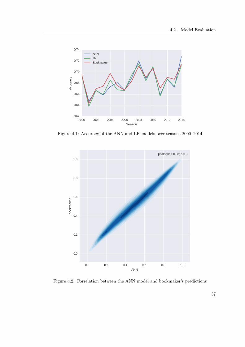
4.2. Model Evaluation

Figure 4.1: Accuracy of the ANN and LR models over seasons 2000–2014

Figure 4.2: Correlation between the ANN model and bookmaker’s predictions

37

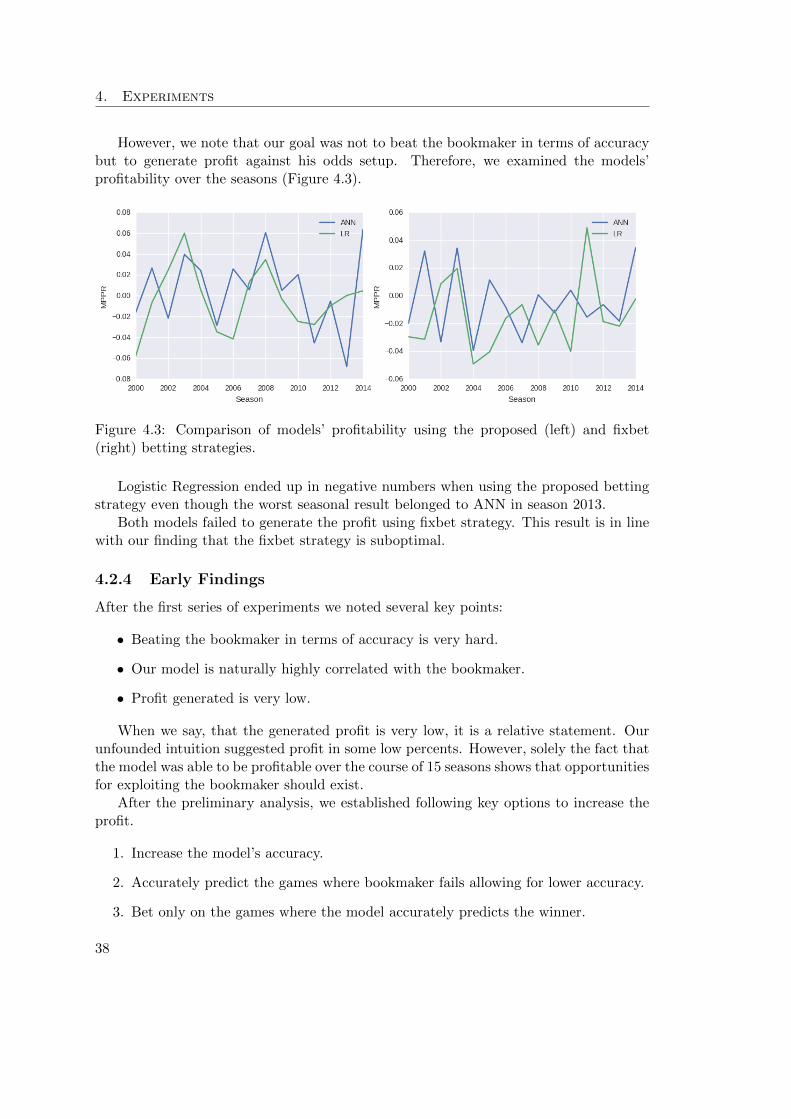
4. Experiments

However, we note that our goal was not to beat the bookmaker in terms of accuracybut to generate profit against his odds setup. Therefore, we examined the models’profitability over the seasons (Figure 4.3).

Figure 4.3: Comparison of models’ profitability using the proposed (left) and fixbet(right) betting strategies.

Logistic Regression ended up in negative numbers when using the proposed bettingstrategy even though the worst seasonal result belonged to ANN in season 2013.

Both models failed to generate the profit using fixbet strategy. This result is in linewith our finding that the fixbet strategy is suboptimal.

4.2.4 Early Findings

After the first series of experiments we noted several key points:

• Beating the bookmaker in terms of accuracy is very hard.

• Our model is naturally highly correlated with the bookmaker.

• Profit generated is very low.

When we say, that the generated profit is very low, it is a relative statement. Ourunfounded intuition suggested profit in some low percents. However, solely the fact thatthe model was able to be profitable over the course of 15 seasons shows that opportunitiesfor exploiting the bookmaker should exist.

After the preliminary analysis, we established following key options to increase theprofit.

1. Increase the model’s accuracy.

2. Accurately predict the games where bookmaker fails allowing for lower accuracy.

3. Bet only on the games where the model accurately predicts the winner.

38

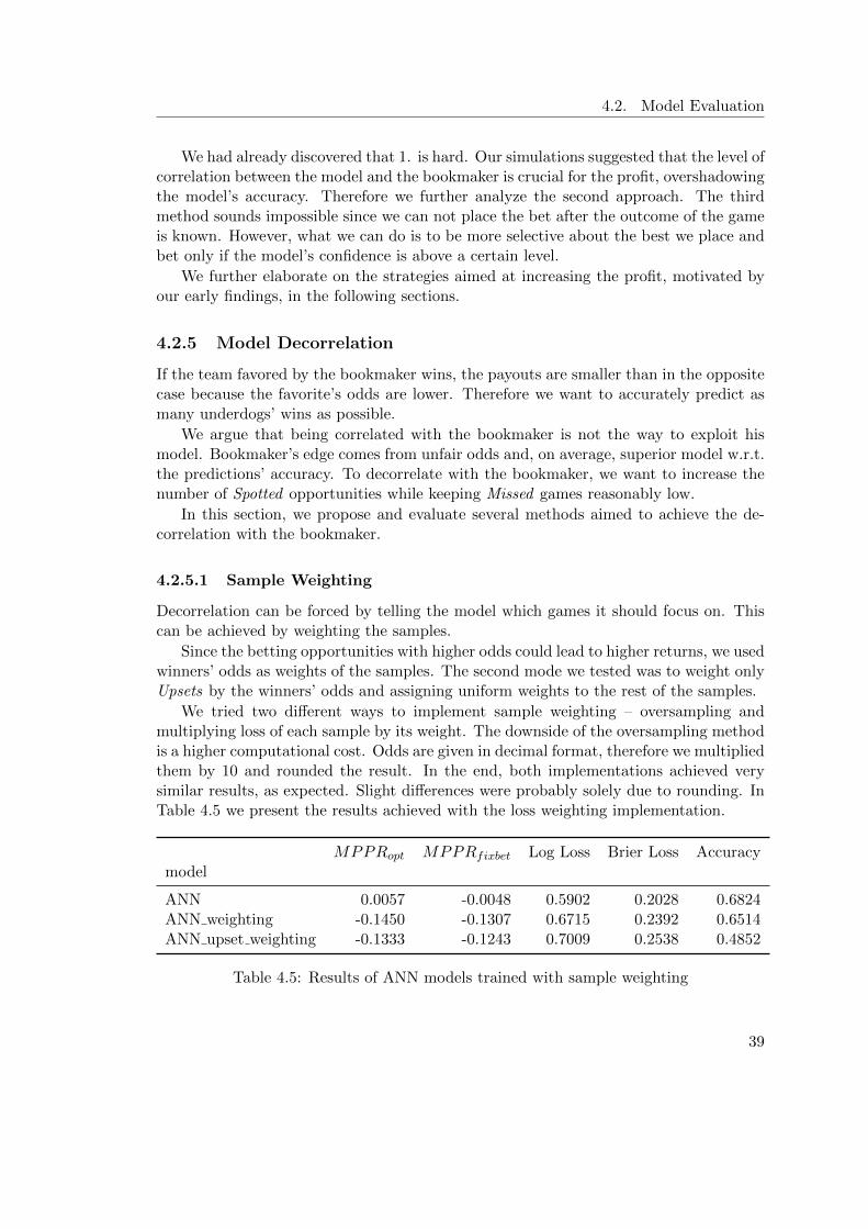
4.2. Model Evaluation

We had already discovered that 1. is hard. Our simulations suggested that the level ofcorrelation between the model and the bookmaker is crucial for the profit, overshadowingthe model’s accuracy. Therefore we further analyze the second approach. The thirdmethod sounds impossible since we can not place the bet after the outcome of the gameis known. However, what we can do is to be more selective about the best we place andbet only if the model’s confidence is above a certain level.

We further elaborate on the strategies aimed at increasing the profit, motivated byour early findings, in the following sections.

4.2.5 Model Decorrelation

If the team favored by the bookmaker wins, the payouts are smaller than in the oppositecase because the favorite’s odds are lower. Therefore we want to accurately predict asmany underdogs’ wins as possible.

We argue that being correlated with the bookmaker is not the way to exploit hismodel. Bookmaker’s edge comes from unfair odds and, on average, superior model w.r.t.the predictions’ accuracy. To decorrelate with the bookmaker, we want to increase thenumber of Spotted opportunities while keeping Missed games reasonably low.

In this section, we propose and evaluate several methods aimed to achieve the de-correlation with the bookmaker.

4.2.5.1 Sample Weighting

Decorrelation can be forced by telling the model which games it should focus on. Thiscan be achieved by weighting the samples.

Since the betting opportunities with higher odds could lead to higher returns, we usedwinners’ odds as weights of the samples. The second mode we tested was to weight onlyUpsets by the winners’ odds and assigning uniform weights to the rest of the samples.

We tried two different ways to implement sample weighting – oversampling andmultiplying loss of each sample by its weight. The downside of the oversampling methodis a higher computational cost. Odds are given in decimal format, therefore we multipliedthem by 10 and rounded the result. In the end, both implementations achieved verysimilar results, as expected. Slight differences were probably solely due to rounding. InTable 4.5 we present the results achieved with the loss weighting implementation.

MPPRopt MPPRfixbet Log Loss Brier Loss Accuracymodel

ANN 0.0057 -0.0048 0.5902 0.2028 0.6824ANN weighting -0.1450 -0.1307 0.6715 0.2392 0.6514ANN upset weighting -0.1333 -0.1243 0.7009 0.2538 0.4852

Table 4.5: Results of ANN models trained with sample weighting

39

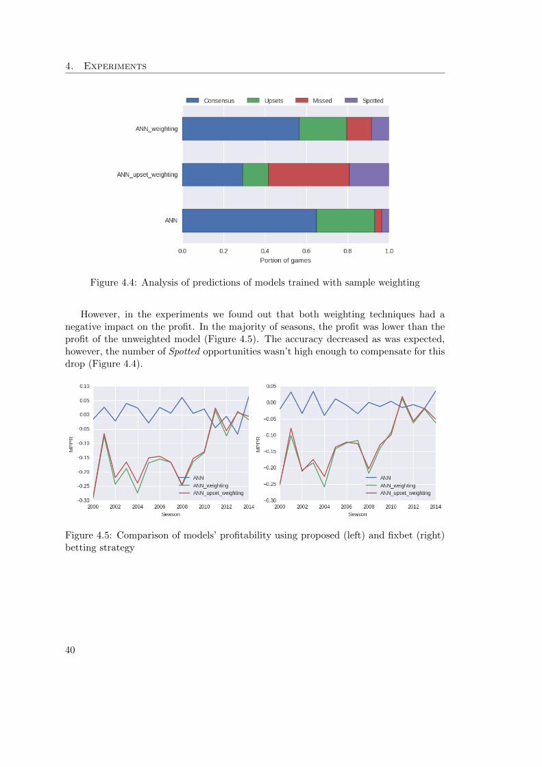
4. Experiments

Figure 4.4: Analysis of predictions of models trained with sample weighting

However, in the experiments we found out that both weighting techniques had anegative impact on the profit. In the majority of seasons, the profit was lower than theprofit of the unweighted model (Figure 4.5). The accuracy decreased as was expected,however, the number of Spotted opportunities wasn’t high enough to compensate for thisdrop (Figure 4.4).

Figure 4.5: Comparison of models’ profitability using proposed (left) and fixbet (right)betting strategy

40

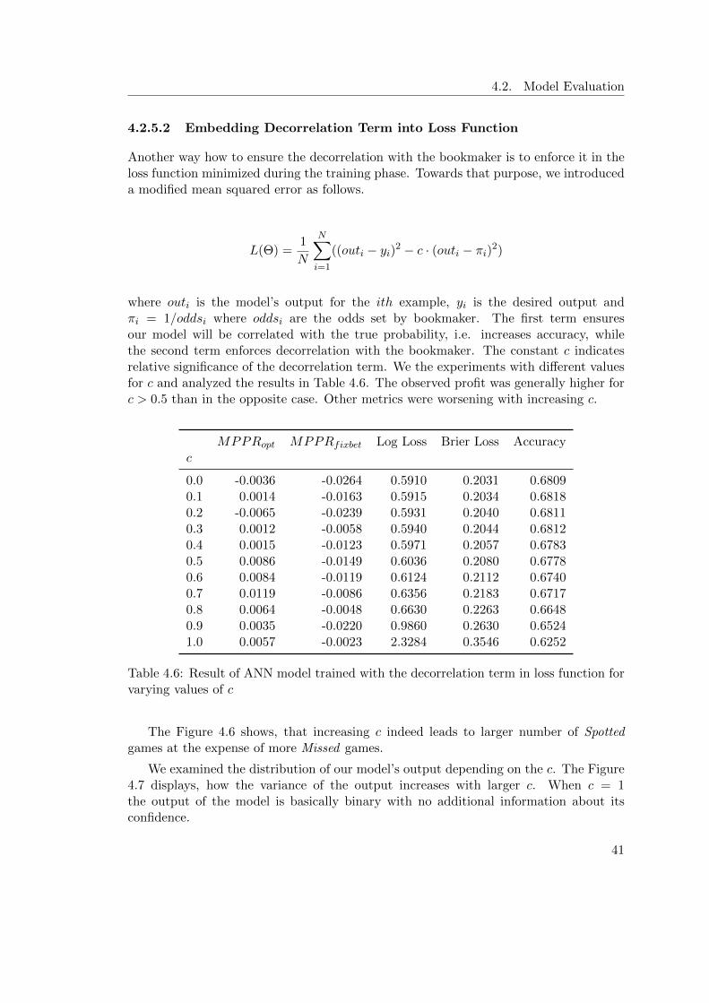
4.2. Model Evaluation

4.2.5.2 Embedding Decorrelation Term into Loss Function

Another way how to ensure the decorrelation with the bookmaker is to enforce it in theloss function minimized during the training phase. Towards that purpose, we introduceda modified mean squared error as follows.

L(Θ) =1

N

N∑i=1

((outi − yi)2 − c · (outi − πi)2)

where outi is the model’s output for the ith example, yi is the desired output andπi = 1/oddsi where oddsi are the odds set by bookmaker. The first term ensuresour model will be correlated with the true probability, i.e. increases accuracy, whilethe second term enforces decorrelation with the bookmaker. The constant c indicatesrelative significance of the decorrelation term. We the experiments with different valuesfor c and analyzed the results in Table 4.6. The observed profit was generally higher forc > 0.5 than in the opposite case. Other metrics were worsening with increasing c.

MPPRopt MPPRfixbet Log Loss Brier Loss Accuracyc

0.0 -0.0036 -0.0264 0.5910 0.2031 0.68090.1 0.0014 -0.0163 0.5915 0.2034 0.68180.2 -0.0065 -0.0239 0.5931 0.2040 0.68110.3 0.0012 -0.0058 0.5940 0.2044 0.68120.4 0.0015 -0.0123 0.5971 0.2057 0.67830.5 0.0086 -0.0149 0.6036 0.2080 0.67780.6 0.0084 -0.0119 0.6124 0.2112 0.67400.7 0.0119 -0.0086 0.6356 0.2183 0.67170.8 0.0064 -0.0048 0.6630 0.2263 0.66480.9 0.0035 -0.0220 0.9860 0.2630 0.65241.0 0.0057 -0.0023 2.3284 0.3546 0.6252

Table 4.6: Result of ANN model trained with the decorrelation term in loss function forvarying values of c

The Figure 4.6 shows, that increasing c indeed leads to larger number of Spottedgames at the expense of more Missed games.

We examined the distribution of our model’s output depending on the c. The Figure4.7 displays, how the variance of the output increases with larger c. When c = 1the output of the model is basically binary with no additional information about itsconfidence.

41

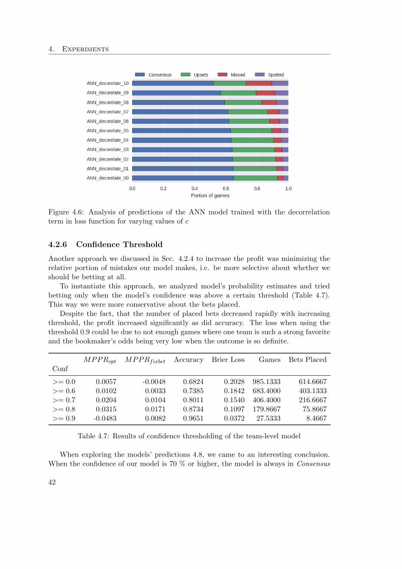
4. Experiments

Figure 4.6: Analysis of predictions of the ANN model trained with the decorrelationterm in loss function for varying values of c

4.2.6 Confidence Threshold

Another approach we discussed in Sec. 4.2.4 to increase the profit was minimizing therelative portion of mistakes our model makes, i.e. be more selective about whether weshould be betting at all.

To instantiate this approach, we analyzed model’s probability estimates and triedbetting only when the model’s confidence was above a certain threshold (Table 4.7).This way we were more conservative about the bets placed.

Despite the fact, that the number of placed bets decreased rapidly with increasingthreshold, the profit increased significantly as did accuracy. The loss when using thethreshold 0.9 could be due to not enough games where one team is such a strong favoriteand the bookmaker’s odds being very low when the outcome is so definite.

MPPRopt MPPRfixbet Accuracy Brier Loss Games Bets PlacedConf

>= 0.0 0.0057 -0.0048 0.6824 0.2028 985.1333 614.6667>= 0.6 0.0102 0.0033 0.7385 0.1842 683.4000 403.1333>= 0.7 0.0204 0.0104 0.8011 0.1540 406.4000 216.6667>= 0.8 0.0315 0.0171 0.8734 0.1097 179.8667 75.8667>= 0.9 -0.0483 0.0082 0.9651 0.0372 27.5333 8.4667

Table 4.7: Results of confidence thresholding of the team-level model

When exploring the models’ predictions 4.8, we came to an interesting conclusion.When the confidence of our model is 70 % or higher, the model is always in Consensus

42

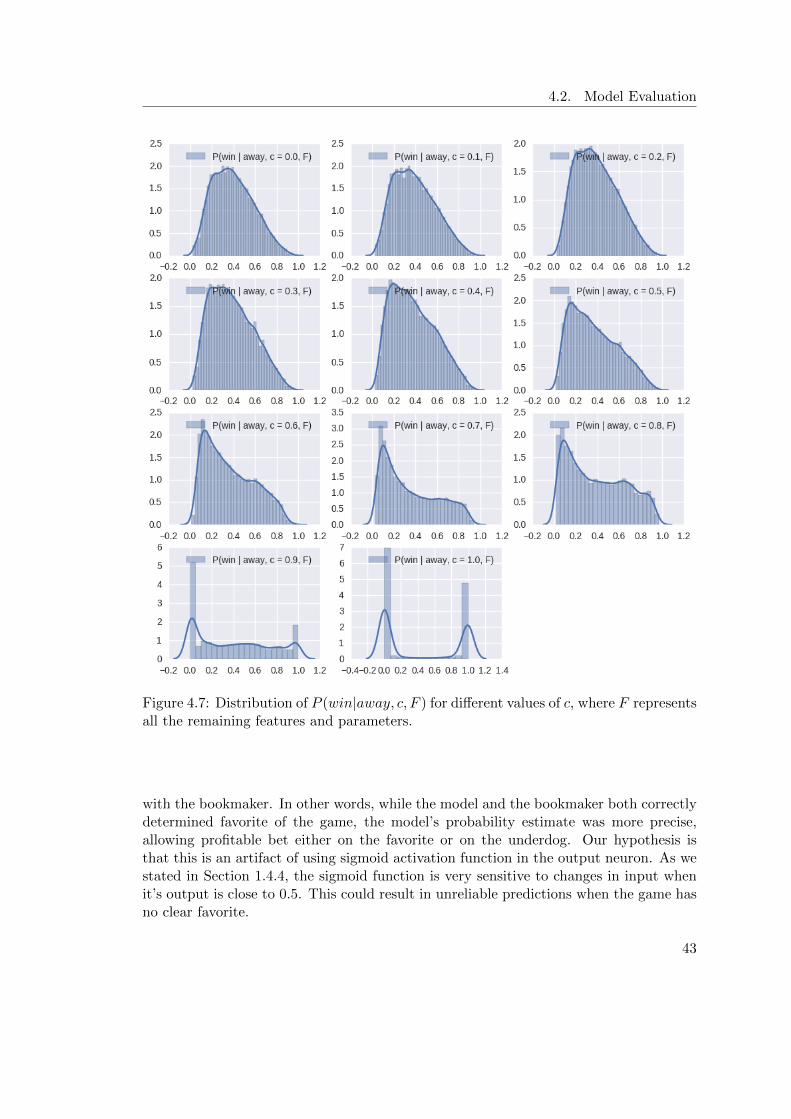
4.2. Model Evaluation

Figure 4.7: Distribution of P (win|away, c, F ) for different values of c, where F representsall the remaining features and parameters.

with the bookmaker. In other words, while the model and the bookmaker both correctlydetermined favorite of the game, the model’s probability estimate was more precise,allowing profitable bet either on the favorite or on the underdog. Our hypothesis isthat this is an artifact of using sigmoid activation function in the output neuron. As westated in Section 1.4.4, the sigmoid function is very sensitive to changes in input whenit’s output is close to 0.5. This could result in unreliable predictions when the game hasno clear favorite.

43

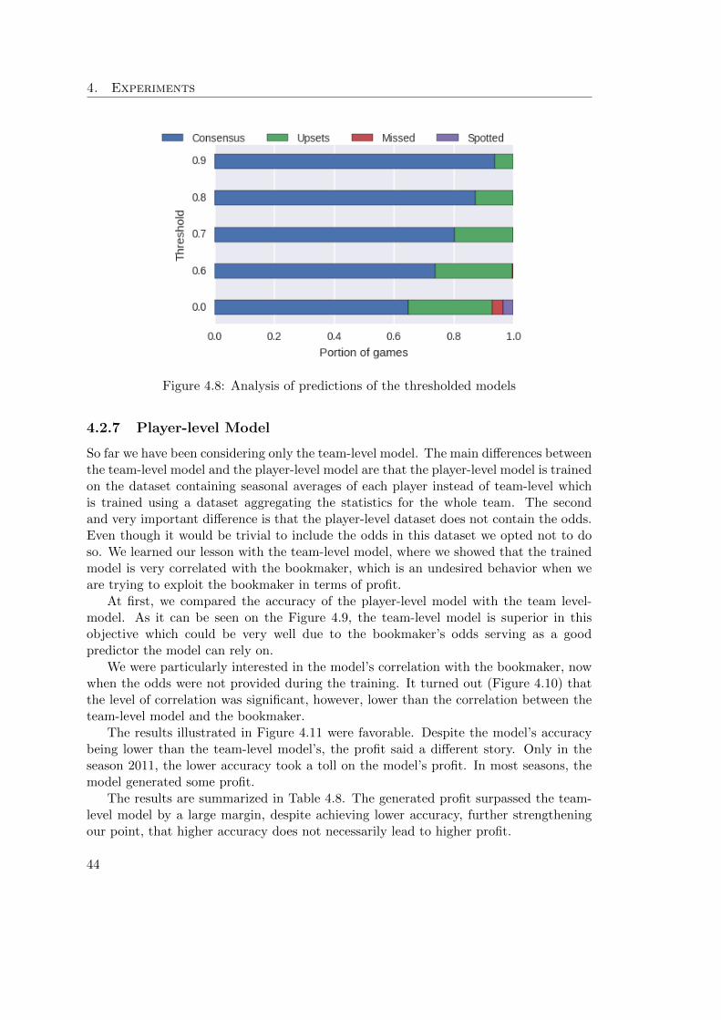
4. Experiments

Figure 4.8: Analysis of predictions of the thresholded models

4.2.7 Player-level Model

So far we have been considering only the team-level model. The main differences betweenthe team-level model and the player-level model are that the player-level model is trainedon the dataset containing seasonal averages of each player instead of team-level whichis trained using a dataset aggregating the statistics for the whole team. The secondand very important difference is that the player-level dataset does not contain the odds.Even though it would be trivial to include the odds in this dataset we opted not to doso. We learned our lesson with the team-level model, where we showed that the trainedmodel is very correlated with the bookmaker, which is an undesired behavior when weare trying to exploit the bookmaker in terms of profit.

At first, we compared the accuracy of the player-level model with the team level-model. As it can be seen on the Figure 4.9, the team-level model is superior in thisobjective which could be very well due to the bookmaker’s odds serving as a goodpredictor the model can rely on.

We were particularly interested in the model’s correlation with the bookmaker, nowwhen the odds were not provided during the training. It turned out (Figure 4.10) thatthe level of correlation was significant, however, lower than the correlation between theteam-level model and the bookmaker.

The results illustrated in Figure 4.11 were favorable. Despite the model’s accuracybeing lower than the team-level model’s, the profit said a different story. Only in theseason 2011, the lower accuracy took a toll on the model’s profit. In most seasons, themodel generated some profit.

The results are summarized in Table 4.8. The generated profit surpassed the team-level model by a large margin, despite achieving lower accuracy, further strengtheningour point, that higher accuracy does not necessarily lead to higher profit.

44

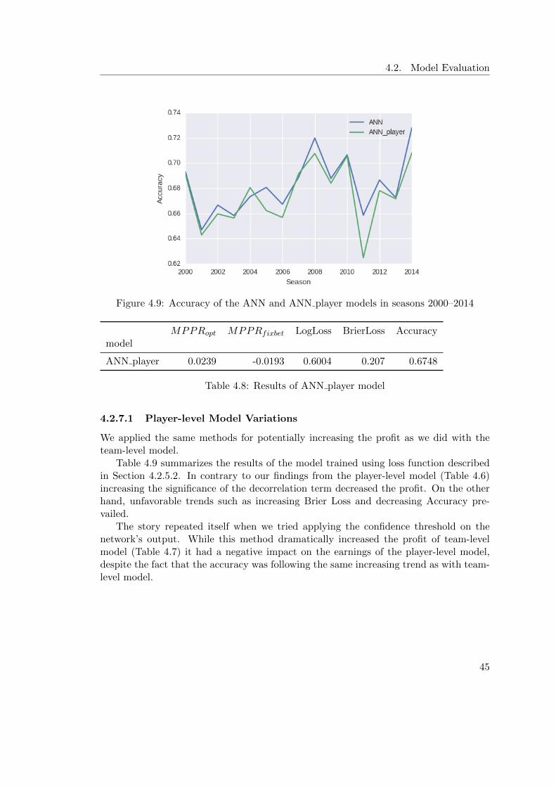
4.2. Model Evaluation

Figure 4.9: Accuracy of the ANN and ANN player models in seasons 2000–2014

MPPRopt MPPRfixbet LogLoss BrierLoss Accuracymodel

ANN player 0.0239 -0.0193 0.6004 0.207 0.6748

Table 4.8: Results of ANN player model

4.2.7.1 Player-level Model Variations

We applied the same methods for potentially increasing the profit as we did with theteam-level model.

Table 4.9 summarizes the results of the model trained using loss function describedin Section 4.2.5.2. In contrary to our findings from the player-level model (Table 4.6)increasing the significance of the decorrelation term decreased the profit. On the otherhand, unfavorable trends such as increasing Brier Loss and decreasing Accuracy pre-vailed.

The story repeated itself when we tried applying the confidence threshold on thenetwork’s output. While this method dramatically increased the profit of team-levelmodel (Table 4.7) it had a negative impact on the earnings of the player-level model,despite the fact that the accuracy was following the same increasing trend as with team-level model.

45

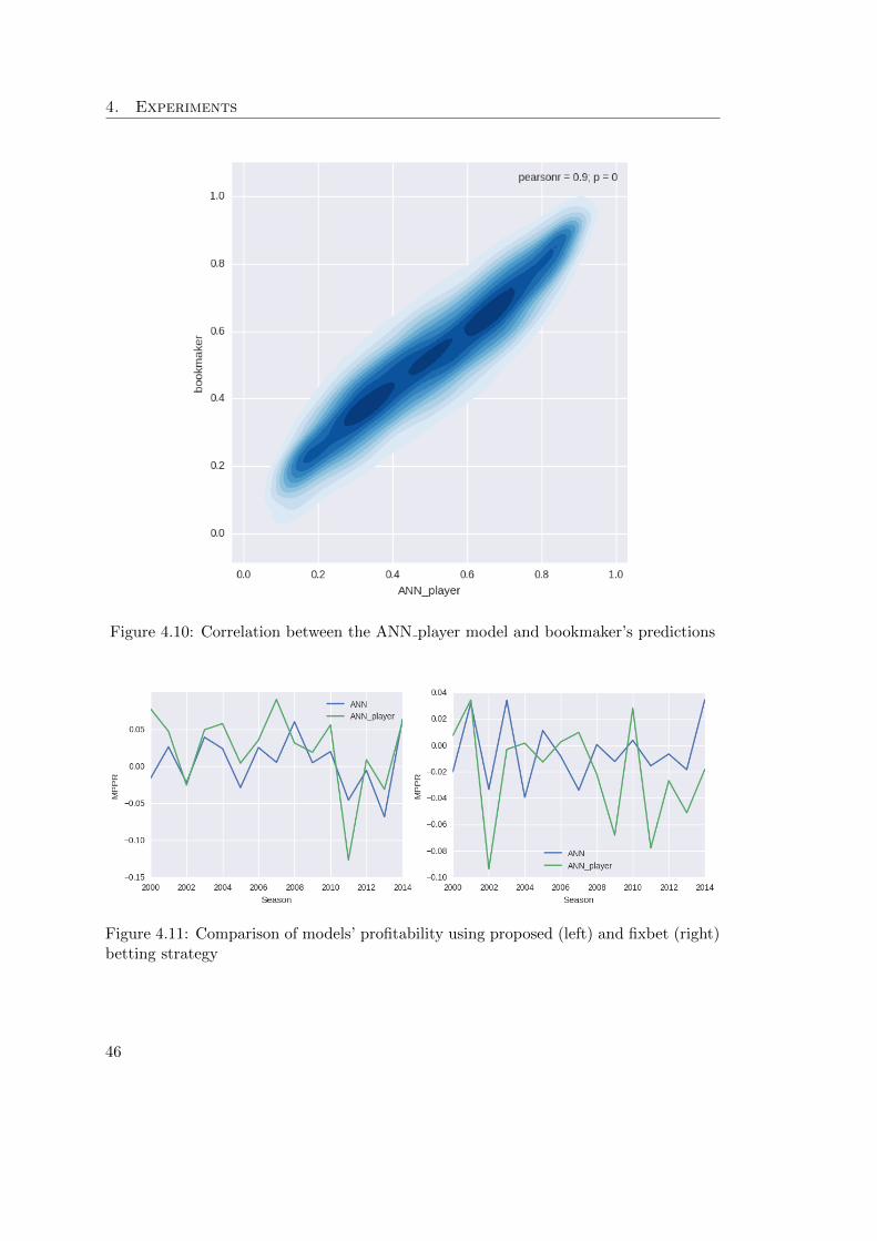
4. Experiments

Figure 4.10: Correlation between the ANN player model and bookmaker’s predictions

Figure 4.11: Comparison of models’ profitability using proposed (left) and fixbet (right)betting strategy

46

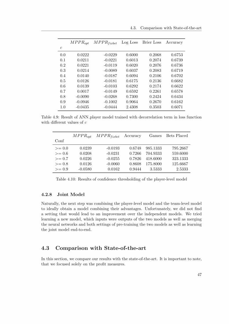
4.3. Comparison with State-of-the-art

MPPRopt MPPRfixbet Log Loss Brier Loss Accuracyc

0.0 0.0222 -0.0229 0.6000 0.2068 0.67530.1 0.0211 -0.0221 0.6013 0.2074 0.67390.2 0.0221 -0.0119 0.6020 0.2076 0.67360.3 0.0214 -0.0089 0.6037 0.2083 0.67190.4 0.0140 -0.0187 0.6094 0.2106 0.67020.5 0.0126 -0.0181 0.6175 0.2136 0.66820.6 0.0139 -0.0103 0.6292 0.2174 0.66220.7 0.0017 -0.0149 0.6592 0.2261 0.65780.8 -0.0090 -0.0268 0.7300 0.2424 0.64340.9 -0.0946 -0.1002 0.9064 0.2670 0.61621.0 -0.0435 -0.0444 2.4308 0.3503 0.6071

Table 4.9: Result of ANN player model trained with decorrelation term in loss functionwith different values of c

MPPRopt MPPRfixbet Accuracy Games Bets PlacedConf

>= 0.0 0.0239 -0.0193 0.6748 985.1333 795.2667>= 0.6 0.0208 -0.0231 0.7266 704.9333 559.6000>= 0.7 0.0226 -0.0255 0.7826 418.6000 323.1333>= 0.8 0.0126 -0.0060 0.8608 175.8000 125.6667>= 0.9 -0.0580 0.0162 0.9444 3.5333 2.5333

Table 4.10: Results of confidence thresholding of the player-level model

4.2.8 Joint Model

Naturally, the next step was combining the player-level model and the team-level modelto ideally obtain a model combining their advantages. Unfortunately, we did not finda setting that would lead to an improvement over the independent models. We triedlearning a new model, which inputs were outputs of the two models as well as mergingthe neural networks and both settings of pre-training the two models as well as learningthe joint model end-to-end.

4.3 Comparison with State-of-the-art

In this section, we compare our results with the state-of-the-art. It is important to note,that we focused solely on the profit measures.

47

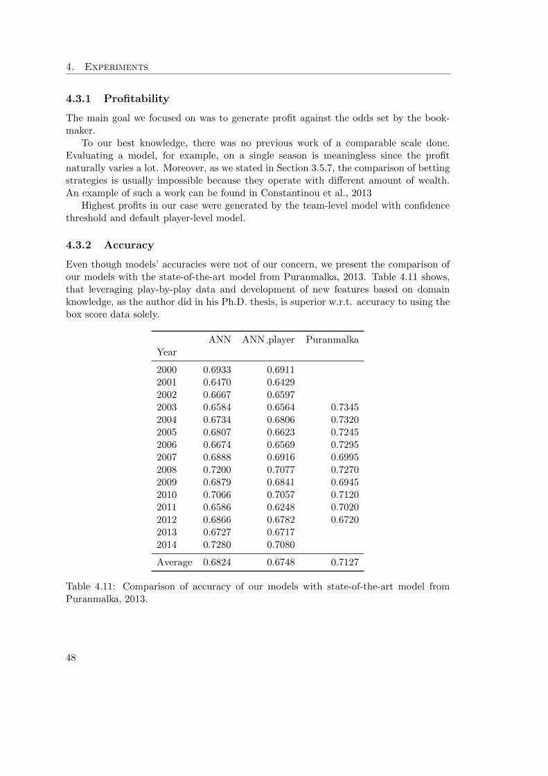
4. Experiments

4.3.1 Profitability

The main goal we focused on was to generate profit against the odds set by the book-maker.

To our best knowledge, there was no previous work of a comparable scale done.Evaluating a model, for example, on a single season is meaningless since the profitnaturally varies a lot. Moreover, as we stated in Section 3.5.7, the comparison of bettingstrategies is usually impossible because they operate with different amount of wealth.An example of such a work can be found in Constantinou et al., 2013

Highest profits in our case were generated by the team-level model with confidencethreshold and default player-level model.

4.3.2 Accuracy

Even though models’ accuracies were not of our concern, we present the comparison ofour models with the state-of-the-art model from Puranmalka, 2013. Table 4.11 shows,that leveraging play-by-play data and development of new features based on domainknowledge, as the author did in his Ph.D. thesis, is superior w.r.t. accuracy to using thebox score data solely.

ANN ANN player PuranmalkaYear

2000 0.6933 0.69112001 0.6470 0.64292002 0.6667 0.65972003 0.6584 0.6564 0.73452004 0.6734 0.6806 0.73202005 0.6807 0.6623 0.72452006 0.6674 0.6569 0.72952007 0.6888 0.6916 0.69952008 0.7200 0.7077 0.72702009 0.6879 0.6841 0.69452010 0.7066 0.7057 0.71202011 0.6586 0.6248 0.70202012 0.6866 0.6782 0.67202013 0.6727 0.67172014 0.7280 0.7080

Average 0.6824 0.6748 0.7127

Table 4.11: Comparison of accuracy of our models with state-of-the-art model fromPuranmalka, 2013.

48

Chapter 5

Conclusion

The goal of our work was to find a way to exploit betting market inefficiencies, i.e. togenerate profit against bookmaker’s odds setup, using machine learning. To the bestof our knowledge, no work of similar scale, focusing on profitability, has been done andmade publicly available before.

Our findings are in agreement with the previous research that the bookmaker is veryhard to beat in terms of accuracy. However, we argued that accuracy is not a directmeasure of profit, and we illustrated the use of Modern Portfolio Theory in the contextof the betting market, allowing us to more formally analyze and compare various bettingstrategies, that are present in the literature, in order to optimize our betting behavior.By focusing explicitly on the profitability, our proposed models were able to generateprofit over the course of the presented 15 seasons of NBA records.

We further argued that models’ correlation with the bookmaker plays a crucialrole when considering the profit, overshadowing the importance of accuracy. Severalstrategies on how to achieve decorrelation with the bookmaker were tested to confirmour assumption. Enforcing the decorrelation in the loss function used during the train-ing phase and excluding the bookmaker’s odds from the features proved to be the mosteffective approaches.

Another point we made is that the bettors can leverage their choice not to bet whenthe model’s confidence in the outcome is low. Being more conservative about placingthe bets turned out to be a feasible solution for generating the profit even while beingcorrelated with the bookmaker.

Experiments with our proposed neural architectures demonstrated, that by aggrega-tion of player-level statistics by a self-learned function, in our case a convolutional filter,we can obtain highly useful latent features, often beating the standard, expert designedstatistical indicators on the team level.

49

5. Conclusion

5.1 Future Work

The scope of future work is naturally very broad and covers most of the parts of thedescribed pipeline.

We have experimented with training the models with customized loss function usingthe decorrelation term. Although this modification proved useful, we believe that theremight be more suitable loss functions with the same goal we have not yet discovered.It is also not clear, which betting strategy to use when the output of the network isaffected by the decorrelation term in the loss function.

We do not claim the used Mean Portfolio Theory to be flawless. We acknowledgedthe drawback of using the variance of the profit as a measure of risk. Other measuresfor the risk could also be explored.

As we already mentioned, our dataset consisted solely of the seasonal averages. Re-current neural networks or other techniques could be used to leverage the time-seriescharacteristics of the seasons.

Another challenge is to find an efficient way of combining the player-level and theteam-level model.

To further validate our findings, experiments on different sub-domains (sport) ordifferent types of bets (f.e. proposition bets) should be done. Another validation can bedone by evaluating the models in the upcoming seasons.

50

Bibliography

ARKES, Jeremy; MARTINEZ, Jose, 2011. Finally, Evidence for a Momentum Effect inthe NBA. Journal of Quantitative Analysis in Sports. Vol. 7, no. 3, pp. Article 13.

BAR-ELI, Michael; AVUGOS, Simcha; RAAB, Markus, 2006. Twenty years of “hothand” research: Review and critique. Psychology of Sport and Exercise. Vol. 7, no.6, pp. 525–553.

CONSTANTINOU, Anthony Costa; FENTON, Norman Elliott; NEIL, Martin, 2013.Profiting from an inefficient association football gambling market: Prediction, riskand uncertainty using Bayesian networks. Knowledge-Based Systems. Vol. 50, pp.60–86.

FORREST, David; GODDARD, John; SIMMONS, Robert, 2005. Odds-setters as fore-casters: The case of English football. International Journal of Forecasting. Vol. 21,no. 3, pp. 551–564.

FRANCK, Egon; VERBEEK, Erwin; NUESCH, Stephan, 2010. Prediction accuracy ofdifferent market structures - bookmakers versus a betting exchange. InternationalJournal of Forecasting. Vol. 26, no. 3, pp. 448–459.

FRANCK, Egon; VERBEEK, Erwin; NUESCH, Stephan, 2009. Inter-market arbitragein sports betting. Technical report. National Centre for Econometric Research.

GODDARD, John; ASIMAKOPOULOS, Ioannis, 2004. Forecasting football results andthe efficiency of fixed-odds betting. Journal of Forecasting. Vol. 23, no. 1, pp. 51–66.

GOODFELLOW, Ian; BENGIO, Yoshua; COURVILLE, Aaron, 2016. Deep Learning.MIT Press. http://www.deeplearningbook.org.

HAGHIGHAT, Maral; RASTEGARI, Hamid; NOURAFZA, Nasim, 2013. A Reviewof Data Mining Techniques for Result Prediction in Sports. Advances in ComputerScience. Vol. 2, no. 5, pp. 7–12.

HVATTUM, Lars Magnus; ARNTZEN, Halvard, 2010. Using ELO ratings for matchresult prediction in association football. International Journal of Forecasting. Vol. 26,no. 3, pp. 460–470.

51

Bibliography

IBANEZ, Sergio J; GARCIA, Javier; FEU, Sebastian; LORENZO, Alberto; SAMPAIO,Jaime, 2009. Effects of consecutive basketball games on the game-related statisticsthat discriminate winner and losing teams. Journal of Sports Science and Medicine.Vol. 8, no. 3, pp. 458–462.

IBANEZ, Sergio J.; SAMPAIO, Jaime; FEU, Sebastian; LORENZO, Alberto; GOMEZ,Miguel a.; ORTEGA, Enrique, 2008. Basketball game-related statistics that discrim-inate between teams’ season-long success. European Journal of Sport Science. Vol. 8,no. 6, pp. 369–372.

IVANKOVIC, Z; RACKOVIC, M; MARKOSKI, B; RADOSAV, D; IVKOVIC, M, 2010.Analysis of basketball games using neural networks. Computational Intelligence andInformatics (CINTI), 2010 11th International Symposium, pp. 251–256.

KAIN, Kyle J.; LOGAN, Trevon D., 2014. Are Sports Betting Markets Prediction Mar-kets?: Evidence From a New Test. Journal of Sports Economics. Vol. 15, no. 1, pp.45–63.

KUBATKO, Justin; OLIVER, Dean; PELTON, Kevin; ROSENBAUM, Dan T, 2007. AStarting Point for Analyzing Basketball Statistics. Journal of Quantitative Analysisin Sports. Vol. 3, no. 3, pp. 1–22.

LEVITT, Steven D., 2004. Why are gambling markets organised so differently fromfinancial markets? Economic Journal. Vol. 114, no. 495, pp. 223–246.

LOEFFELHOLZ, Bernard; BEDNAR, Earl; BAUER, Kenneth W, 2009. PredictingNBA Games Using Neural Networks. Journal of Quantitative Analysis in Sports.Vol. 5, no. 1, pp. 15.

MARKOWITZ, Harry, 1952. Portfolio selection. The journal of finance. Vol. 7, no. 1,pp. 77–91.

MILJKOVIC, Dragan; GAJIC, Ljubisa; KOVACEVIC, Aleksandar; KONJOVIC, Zora,2010. The use of data mining for basketball matches outcomes prediction. In: Intel-ligent Systems and Informatics (SISY), 2010 8. IEEE 8th International Symposiumon Intelligent Systems and Informatics. IEEE, pp. 309–312.

ORR, Genevieve B; MULLER, Klaus-Robert, 2003. Neural networks: tricks of the trade.Springer.

PAUL, Rodney J; WEINBACH, Andrew P., 2007. Does Sportsbook.com set pointspreadsto maximize profits? Tests of the Levitt model of Sportsbook behavior. The Journalof Prediction Markets. Vol. 1, no. 3, pp. 209–218.

PAUL, Rodney J.; WEINBACH, Andrew P., 2008. Price setting in the nba gamblingmarket: Tests of the levitt model of sportsbook behavior. International Journal ofSport Finance. Vol. 3, no. 3, pp. 137–145.

PAUL, Rodney J; WEINBACH, Andrew P, 2010. The determinants of betting volumefor sports in North America: Evidence of sports betting as consumption in the NBAand NHL. International Journal of Sport Finance. Vol. 5, no. 2, pp. 128.

52

Bibliography

PURANMALKA, Keshav (MIT), 2013. Modelling the NBA to Make Better Predictions.Massachusetts Institute of Technology. PhD thesis. Massachusetts Institute of Tech-nology.

SAMPAIO, Jaime; DRINKWATER, Eric J.; LEITE, Nuno M., 2010. Effects of seasonperiod, team quality, and playing time on basketball players’ game-related statistics.European Journal of Sport Science. Vol. 10, no. 2, pp. 141–149.

SHARPE, William F, 1994. The sharpe ratio. The journal of portfolio management.Vol. 21, no. 1, pp. 49–58.

SHIN, Hyun Song, 1991. Optimal betting odds against insider traders. The EconomicJournal. Vol. 101, no. 408, pp. 1179–1185.

SIMMONS, Robert; FORREST, David, 2000. Forecasting sport: the behaviour and per-formance of football tipsters. International Journal of Forecasting. Vol. 16, no. 3, pp.317–331.

SINHA, Shiladitya; DYER, Chris; GIMPEL, Kevin; SMITH, Noah A., 2013. Predictingthe NFL using Twitter. ECML/PKDD 2013 Workshop on Maching Learning andData Mining for Sports Analytics, pp. 1–11. Available from arXiv: 1310.6998.

SIRE, Clement; REDNER, Sidney, 2009. Understanding baseball team standings andstreaks. The European Physical Journal B. Vol. 67, no. 3, pp. 473–481.

SONG, ChiUng; BOULIER, Bryan L.; STEKLER, Herman O., 2007. The comparativeaccuracy of judgmental and model forecasts of American football games. Interna-tional Journal of Forecasting. Vol. 23, no. 3, pp. 405–413.

SPANN, Martin; SKIERA, Bernd, 2009. Journal of Forecasting. Vol. 28, Sports forecast-ing: A comparison of the forecast accuracy of prediction markets, betting odds andtipsters. John Wiley & Sons, Ltd. No. 1.

SRIVASTAVA, Nitish; HINTON, Geoffrey E; KRIZHEVSKY, Alex; SUTSKEVER, Ilya;SALAKHUTDINOV, Ruslan, 2014. Dropout: a simple way to prevent neural net-works from overfitting. Journal of Machine Learning Research. Vol. 15, no. 1, pp.1929–1958.

STEKLER, H. O.; SENDOR, David; VERLANDER, Richard, 2010. Issues in sportsforecasting. International Journal of Forecasting. Vol. 26, no. 3, pp. 606–621.

STRUMBELJ, Erik, 2014. On determining probability forecasts from betting odds. In-ternational Journal of Forecasting. Vol. 30, no. 4, pp. 934–943.

VERGIN, Roger, 2000. Winning streaks in sports and the mispreception of momentum.Journal of Sport Behavior. Vol. 23, no. 2, pp. 181.

VRACAR, Petar; STRUMBELJ, Erik; KONONENKO, Igor, 2016. Modeling basketballplay-by-play data. Expert Systems with Applications. Vol. 44, pp. 58–66.

YANG, Yuanhao, 2015. Predicting Regular Season Results of NBA Teams Based onRegression Analysis of Common Basketball Statistics. Available from arXiv: arXiv:1011.1669v3. PhD thesis.

53

Bibliography

ZIMMERMANN, Albrecht; MOORTHY, Sruthi; SHI, Zifan, 2013. Predicting collegebasketball match outcomes using machine learning techniques: some results and les-sons learned. Available from arXiv: 1310.3607.

54

Appendix A

Features’ descriptions

In this section, we present all the features we used. The grouping, abbreviation anddescription matches the source of the data – stats.nba.com. The grouping of the featuresis following:

basic the very basic statistics such as number of assist etc.

advanced more advanced statistics such as player ratings

four factors described in Kubatko et al., 2007 provide breakdown of the ratings

scoring percentages tied to players scoring

misc other statistics

55

A.

Features’

desc

riptions

Group Feature Description

advanced AST PCT Assist Percentage is the percent of teammate’s field goals that the playerassisted.

advanced AST RATIO Assist Ratio is the number of assists a player or team averages per 100 of theirown possessions.

advanced AST TOV The number of assists a player has for every turnover that player commits.advanced DEF RATING The number of points allowed per 100 possessions by a team. For a player, it

is the number of points per 100 possessions that the team allows while thatindividual player is on the court.

advanced DREB PCT The percentage of defensive rebounds a player or team obtains while on thecourt.

advanced EFG PCT Effective Field Goal Percentage is a field goal percentage that is adjusted formade 3 pointers being 1.5 times more valuable than a 2 point shot.

advanced NET RATING Net Rating is the difference in a player or team’s Offensive and DefensiveRating. The formula for this is: Offensive Rating-Defensive Rating.

advanced OFF RATING The number of points scored per 100 possessions by a team. For a player, itis the number of points per 100 possessions that the team scores while thatindividual player is on the court.

advanced OREB PCT The percentage of offensive rebounds a player or team obtains while on thecourt.

advanced PACE Pace is the number of possessions per 48 minutes for a player or team.advanced PIE PIE is an estimate of a player’s or team’s contributions and impact on a game.

PIE shows what % of game events did that player or team achieve.advanced REB PCT The percentage of total rebounds a player obtains while on the court.advanced TM TOV PCT Turnover Ratio is the number of turnovers a player or team averages per 100

of their own possessions.advanced TS PCT A shooting percentage that is adjusted to include the value three pointers and

free throws. The formula is: Points/ [2*(Field Goals Attempted+0.44*FreeThrows Attempted)]

advanced USG PCT The percentage of a team’s offensive possessions that a player uses while onthe court.

56

basic AST An assist occurs when a player completes a pass to a teammate that directlyleads to a made field goal.

basic BLK A block occurs when an offensive player attempts a shot, and the defenseplayer tips the ball, blocking their chance to score.

basic DREB The number of rebounds a player or team has collected while they were ondefense.

basic FG PCT The percentage of field goals that a player makes. The formula to determinefield goal percentage is: Field Goals Made/Field Goals Attempted.

basic FG3 PCT The percentage of 3 point field goals that a player or team has made.basic FG3A The number of 3 point field goals that a player or team has attempted.basic FG3M The number of 3 point field goals that a player or team has made.basic FGA The number of field goals that a player or team has attempted. This includes

both 2 pointers and 3 pointers.basic FGM The number of field goals that a player or team has made. This includes both

2 pointers and 3 pointers.basic FT PCT The percentage of free throws that a player or team has made.basic FTA The number of free throws that a player or team has taken.basic FTM The number of free throws that a player or team has successfully made.basic MIN The number of minutes a player or team has played.basic OREB The number of rebounds a player or team has collected while they were on

offense.basic PF The total number of fouls that a player or team has committed.basic PLUS MINUS The point differential of the score for a player while on the court. For a team,

it is how much they are winning or losing by.basic PTS The number of points a player or team has scored. A point is scored when a

player makes a basket.basic REB A rebound occurs when a player recovers the ball after a missed shot.basic STL A steal occurs when a defensive player takes the ball from a player on offense,

causing a turnover.basic TO A turnover occurs when the team on offense loses the ball to the defense.57

A.

Features’

desc

riptions

four factors EFG PCT Effective Field Goal Percentage is a field goal percentage that is adjusted formade 3 pointers being 1.5 times more valuable than a 2 point shot.

four factors FTA RATE The number of free throws a team shoots in comparison to the number of shotsthe team attempted. This is a team statistic, measured while the player is onthe court. The formula is Free Throws Attempted/Field Goals Attempted.This statistic shows who is good at drawing fouls and getting to the line.

four factors OPP EFG PT Opponent’s Effective Field Goal Percentage is what the team’s defense forcestheir opponent to shoot. Effective Field Goal Percentage is a field goal per-centage that is adjusted for made 3 pointers being 1.5 times more valuablethan a 2 point shot.

four factors OPP FTA RATE The number of free throws an opposing player or team shoots in comparisonto the number of shots that player or team shoots.

four factors OPP OREB PCT The opponent’s percentage of offensive rebounds a player or team obtainswhile on the court.

four factors OPP TOV PCT Opponent’s Turnover Ratio is the number of turnovers an opposing team av-erages per 100 of their own possessions.

four factors OREB PCT The percentage of offensive rebounds a player or team obtains while on thecourt.

four factors TM TOV PCT Turnover Ratio is the number of turnovers a player or team averages per 100of their own possessions.

misc BLKA The number of field goal attempts by a player or team that was blocked bythe opposing team.

misc OPP PTS 2ND CHANCE The number of points an opposing team scores on a possession when theopposing team rebounds the ball on offense.

misc OPP PTS FB The number of points scored by an opposing player or team while on a fastbreak.

misc OPP PTS OFF TOV The number of points scored by an opposing player or team following aturnover.

misc OPP PTS PAINT The number of points scored by an opposing player or team in the paint.misc PFD The total number of fouls that a player or team has drawn on the other team.

58

misc PTF FB The number of points scored by a player or team while on a fast break.misc PTS 2ND CHANCE The number points scored by a team on a possession that they rebound the

ball on offense.misc PTS OFF TOV The number of points scored by a player or team following an opponent’s

turnover.misc PTS PAINT The number of points scored by a player or team in the paint.scoring PCT AST 2PM The percentage of 2 point field goals made that are assisted by a teammate.scoring PCT AST 3PM The percentage of 3 point field goals made that are assisted by a teammate.scoring PCT AST FGM The percentage of field goals made that are assisted by a teammate.scoring PCT FGA 2PT The percentage of field goals attempted by a player or team that are 2 pointers.scoring PCT FGA 3PT The percentage of field goals attempted by a player or team that are 3 pointers.scoring PCT PTS 2PT The percentage of points scored by a player or team that are 2 pointers.scoring PCT PTS 2PT MR The percentage of points scored by a player or team that are 2 point mid-

range jump shots. Mid-Range Jump Shots are generally jump shots thatoccur within the 3 point line, but not near the rim.

scoring PCT PTS 3PT The percentage of points scored by a player or team that are 3 pointers.scoring PCT PTS FB The percentage of points scored by a player or team that are scored while on

a fast break.scoring PCT PTS FT The percentage of points scored by a player or team that are free throws.scoring PCT PTS OFF TOV The percentage of points scored by a player or team that are scored after

forcing an opponent’s turnover.scoring PCT PTS PAINT The percentage of points scored by a player or team that are scored in the

paint.scoring PCT UAST 2PM The percentage of 2 point field goals that are not assisted by a teammate.scoring PCT UAST 3PM The percentage of 3 point field goals that are not assisted by a teammate.scoring PCT UAST FGM The percentage of field goals that are not assisted by a teammate.odds ODDS Closing odds set by bookmaker.rest REST Number of days since last game.

59

Appendix B

Acronyms

ANN Artificial Neural Network

MPPR Mean Profit per Round

MSE Mean Squared Error

NBA National Basketball Association

NCAA National Collegiate Athletic Association

NFL National Football League

NHL National Hockey League

61

Appendix C

Contents of enclosed CD

src......................................................implementation sourcestext....................................................the thesis text directory

thesis.pdf .................................... the thesis text in PDF formatthesis.tex...................................the thesis text in LaTeX format

63