Embed Size (px)
Citation preview

NASA / CR-1998-208698
Input Shaping to Reduce Solar ArrayStructural Vibrations
Michael J. Doherty and Robert H. Tolson
Joint Institute for Advancement of Flight Sciences
The George Washington University
Langley Research Center, Hampton, Virginia
National Aeronautics and
Space Administration
Langley Research CenterHampton, Virginia 23681-2199
Prepared for Langley Research Centerunder Cooperative Agreement NCC1-104
August 1998

Available from the following:
NASA Center for AeroSpace Information (CASI)7121 Standard Drive
Hanover, MD 2 ! 076-1320
(301) 621-0390
National Technical Information Service (NTIS)5285 Port Royal Road
Springfield, VA 22161-2171(70 _) 487-4650
Abstract
Structural vibrations induced by actuators can be minimized through the effective use
of feedforward input shaping. Actuator commands are convolved with an input shaping
function to yield an equivalent shaped set of actuator commands. The shaped commands
are designed to achieve the desired maneuver and minimize the residual structural
vibrations.
Input shaping was extended for stepper motor actuators through this research. An
input-shaping technique based on pole-zero cancellation was used to modify the Solar
Array Drive Assembly (SADA) stepper motor commands for the NASA/TRW Lewis
satellite. A series of impulses were calculated as the ideal SADA output for vibration
control and were then discretized for use by the SADA actuator. Simulated actuator
torques were used to calculate the linear structural response and resulted in residual
vibrations that were below the magnitude of baseline cases.
The effectiveness of input shaping is limited by the accuracy of the modal
identification of the structural system. Controller robustness to identification errors was
improved by incorporating additional zeros in the input shaping transfer function. The
additional shaper zeros did not require any increased performance from the actuator or
controller, and the resulting feedforward controller reduced residual vibrations to the level
of the exactly modeled input shaper despite the identification errors.
iii

ABSTRACT
Table of Contents
aJe
111
TABLE OF CONTENTS
LIST OF FIGURES
iv
vi
LIST OF TABLES
NOMENCLATURE xi
1 INTRODUCTION
1.1 POLE-ZERO CANCELLATION THEORY
1.2 EXAMPLE OF STRUCTURAL VIBRATION CONTROL: THE LEWIS SPACECRAFT
1.3 OVERVIEW OF RESULTS
2 POLE-ZERO CANCELLATION VIBRATION CONTROL THEORY
2.1 DISCRETE TIME SYSTEM DESCRIPTION
2.2 ROBUSTNESS AND MULTIPLE-MODE CONSIDERATIONS
2.3 TIME DOMAIN IMPLEMENTATION
2.4 EXTENSION OF POLE-ZERO CANCELLATION FOR STEPPER MOTORS
2.5 SELECTION AND IMPLEMENTATION OF V [BRATION CONTROL SEQUENCES
3 EXAMPLE OF STRUCTURAL VIBRATION CONTROL
3.1 OVERVIEW OF LEWIS SPACECRAFT
3.2 LEWIS SPACECRAFT DYNAMIC MODEL
3.3 DETERMINATION OF TARGET MODES
1
2
2
3
6
6
8
11
12
13
17
17
29
33
iv

4 SIMULATIONS AND RESULTS
4.1 JITTER ANALYSIS METHOD
4.2 BASELINE SIMULATIONS AND JITTER ANALYSIS RESULTS
4.3 SHAPED INPUT SIMULATIONS AND RESULTS
4.4 SUMMARY OF RESULTS
5 CONCLUSIONS
5.1 CURRENT RESULTS
5.2 RECOMMENDATIONS FOR FUTURE RESEARCH
REFERENCES
42
42
46
57
79
82
82
83
86
APPENDIX A: STEPPER MOTOR DESCRIPTION
APPENDIX B: MODAL FREQUENCIES OF LEWIS FINITE ELEMENT MODEL
APPENDIX C: COMPARISON OF JITTER ANALYSIS RESULTS
88
95
97
v

FIGURE 2.1 :
FIGURE 2.2:
FIGURE 2.3:
FIGURE 2.4:
FIGURE 2.5:
FIGURE 2.6:
FIGURE 3.1 :
FIGURE 3.2:
FIGURE 3.3:
List of Figures
SYSTEM BLOCK DIAGRAM
EXAMPLE SYSTEM POLES IN THE Z-PLA_
EXAMPLE SYSTEM POLES AND SHAPER ZEROS IN THE Z-PLANE
EXAMPLE IMPULSE AMPLITUDES
EXAMPLE IMPULSE AMPLITUDES AND STEP SEQUENCE APPROXIMATIONS
EXAMPLE TIME -ADJUSTED STEP SEQUENCE APPROXIMATIONS
LEWIS SPACECRAFT
LEWIS SPACECRAFT ORBITAL OPERATIONS
SPACECRAFT DIMENSIONS (INCHES)
FIGURE 3.4: PAYLOAD INSTRUMENT MODULE PLAN VIEW
FIGURE 3.5:
FIGURE 3.6:
FIGURE 3.7:
FIGURE 3.8:
FIGURE 3.9:
FIGURE 3.10:
FIGURE 3.11 :
FIGURE 3.12:
FIGURE 3.13:
FIGURE 3.14:
FIGURE 4.1 :
FIGURE 4.2:
SOLAR ARRAY WING ISOMETRIC VIEW
TYPE 2 STEPPER MOTOR CUT-AWAY VIEW
TYPE 2 STEPPER MOTOR EXTERNAL VIEW
FOuR-DOF STEPPER MOTOR MODEL DIAGRAM
MOTOR STEPPING OPERATION PARAMI: TERS
SADA #1 Y-ROTATION (INPUT) - HSI X-ROTATION (OUTPUT) FRF
SADA #1 Y-ROTATION - HSI X-ROTATION RANKED MODES (1)
SADA #1 Y-ROTATION - HSI X-ROTATION RANKED MODES (2)
PAYLOAD INSTRUMENT X-ROTATION ]"RE MAGNITUDES
PAYLOAD INSTRUMENT Y-ROTATION [ RE MAGNITUDES
JrrrER ANALYSIS EXAMPLE ( 1)
JITIER ANALYSIS EXAMPLE (2)
vi
6
9
10
12
13
13
17
18
21
22
24
25
26
31
32
36
37
38
39
41
44
44

FIGURE4.3:
FIGURE4.4:
FIGURE4.5:
FIGURE4.6:
FIGURE 4.7:
FIGURE 4.8:
FIGURE 4.9:
FIGURE 4.10:
FIGURE 4.11 :
FIGURE 4.12:
FIGURE 4.13:
FIGURE 4.14:
FIGURE 4.15:
FIGURE 4.16:
FIGURE 4.17:
FIGURE 4.18:
FIGURE 4.19:
FIGURE 4.20:
FIGURE 4.21:
FIGURE 4.22:
FIGURE 4.23:
FIGURE 4.24:
FIGURE 4.25:
FIGURE 4.26:
SINGLE STEP TORQUE TIME PROFILE 48
CSRS TORQUE TIME PROFILE, 3.16 PPS 48
HSI X-ROTATION RESPONSE TO CSRS TORQUE INPUT 49
HSI Y-ROTATION RESPONSE TO CSRS TORQUE INPUT 50
MATS TORQUE TIME PROFILE, 200 PPS 52
HSI X-ROTATION RESPONSE TO MATS TORQUE INPUT 53
HSI Y-ROTATION RESPONSE TO MATS TORQUE INPUT 54
HSI X-ROTATION BASELINE JITIER LEVEI__ 55
LEISA X-ROTATION BASELINE JITIER LEVELS 55
HSI Y-ROTATION BASELINE JrlTER LEVELS 56
LEISA Y-ROTATION BASELINE JrlTER LEVELS 56
SYSTEM POLES IN THE Z-PLANE (T= 1.14 SECONDS) 61
SADA TORQUE TIME PROFILE FOR VCS #1 62
HSI X-ROTATION RESPONSE TO VCS #l 63
HSI Y-ROTATION RESPONSE TO VCS #1 64
HSI X-ROTATION J1TrER ANALYSIS RESULTS (3.5-SECOND WINDOW) 67
LEISA X-ROTATION JrrrER ANALYSIS RESULTS (3.5-SECOND WINDOW) 68
HSI Y-ROTATION Jrr'rER ANALYSIS RESULTS (3.5-SECOND WINDOW) 69
LEISA Y-ROTATION JIq'rER ANALYSIS RESULTS (3.5-SECOND WINDOW) 70
SYSTEM POLES AND VCS #2 ZEROS IN THE Z-PLANE (T=1.035 SECONDS) 73
HSI X-ROTATION JrrrER ANALYSIS RESULTS (3.5-SECOND WINDOW) 74
LEISA X-ROTATION JITrER ANALYSIS RESULTS (3.5-SECOND WINDOW) 75
HSI Y-ROTATION JrrTER ANALYSIS RESULTS (3.5-SECOND WINDOW) 76
LEISA Y-ROTATION JITTER ANALYSIS RESULTS (3.5-SECOND WINDOW) 77
vii

FIGURE A. 1 :
FIGURE A.2:
FIGURE A.3:
FIGURE C. 1 :
FIGURE C.2:
FIGURE C.3:
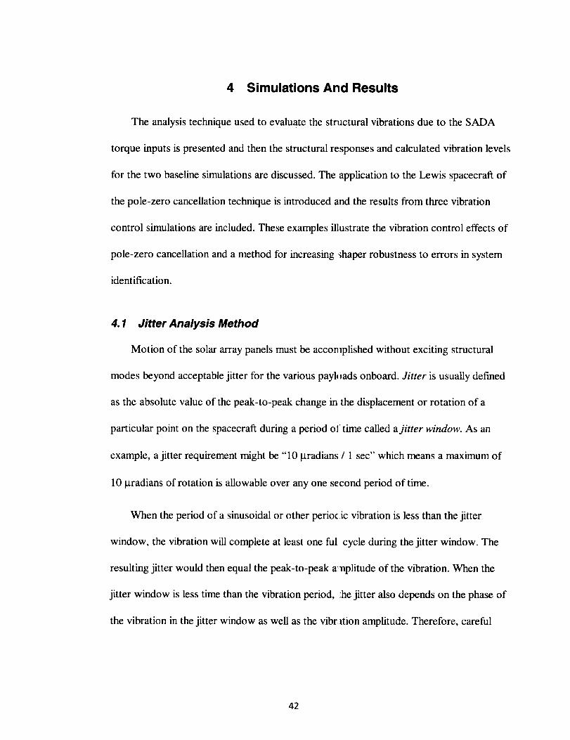
FIGURE C.4:
FIGURE C.5:
FIGURE C.6:
FIGURE C.7:
FIGURE C.8:
FIGURE C.9:
FIGURE C. 10:
FIGURE C. 11 :
FIGURE C. 12:
FIGURE C. 13:
FIGURE C. 14:
FIGURE C. 15:
FIGURE C. 16:
FIGURE C. 17:
FIGURE C. 18:
FIGURE C. 19:
FIGURE C.20:
FIGURE C.21 :
DETENT AND STATE #1 TORQUES VS. ROTOR ELECTRICAL ANGLE 90
COMPOSITE TORQUE VS. ROTOR ELECTRICAL ANGLE 91
DETENT, STATES #1, #2, AND #3 TORQLES VS. ROTOR ELECTRICAL ANGLE 93
HSI X-ROTATION JITrER LEVELS (0.05 SECOND WINDOW) 98
LEISA X-ROTATION JITIER LEVELS (0.05 SECOND WINDOW) 99
HSI X-ROTATION JITTER LEVELS (0.1 SECOND WINDOW) 100
LEISA X-ROTATION JrITER LEVELS (0.1 SECOND WINDOW) 101
HSI X-ROTATION JITTER LEVELS (0.2 SECOND WINDOW) 102
LEISA X-ROTATION JITTER LEVELS (0.2 SECOND WINDOW) 103
HSI X-ROTATION JITTER LEVELS (0.5 SECOND WINDOW) 104
LEISA X-ROTATION JITTER LEVELS (C'.5 SECOND WINDOW) 105
HSI X-ROTATION JrrrER LEVELS (1 SECOND WINDOW) 106
LEISA X-ROTATION JrrrER LEVEES ( 1 SECOND WINDOW) 107
HSI X-ROTATION JrrTER LEVELS (3.5 SECOND WINDOW) 108
LEISA X-ROTATION JrI'rER LEVELS (3.5 SECOND WINDOW) 109
HSI Y-ROTATION JrlTER LEVELS (0.05 SECOND WINDOW) 110
LEISA Y-ROTATION JITTER LEVELS (0.05 SECOND WINDOW) 111
HSI Y-ROTATION JrITER LEVELS (0.1 SECOND WINDOW) 112
LEISA Y-ROTATION JrI'rER LEVELS (). 1 SECOND WINDOW) 113
HSI Y-ROTATION JITYER LEVELS (0.2 SECOND WINDOW) 114
LEISA Y-ROTATION JrlTER LEVELS (0.2 SECOND WINDOW) 115
HSI Y-ROTATION JrlTER LEVELS (0.5 SECOND WINDOW) 116
LEISA Y-ROTATION JITrER LEVEl.S (I).5 SECOND WINDOW) 117
HSI Y-ROTATION Jrr'rER LEVELS (1 SECOND WINDOW) 118
.°.
viii

FIGUREC.22:
FIGUREC.23:
FIGUREC.24:
LEISA Y-ROTATION JITrER LEVELS (1 SECOND WINDOW)
HSI Y-ROTATION JITYER LEVELS (3.5 SECOND WINDOW)
LEISA Y-ROTATION JrlTER LEVELS (3.5 SECOND WINDOW)
119
120
121
ix

TABLE 3.1:
TABLE 3.2:
TABLE 3.3:
TABLE 3.4:
TABLE 3.5:
TABLE 3.6:
TABLE 3.7:
TABLE 4.1 :
TABLE 4.2:
TABLE 4.3:
TABLE 4.4:
TABLE 4.5:
List of Tables
PAYLOAD INSTRUMENT MISSION REQUIREMENTS
LEWIS SPACECRAFT PHYSICAL QUANTmES
TYPE 2 STEPPER MOTOR SPECIFICATIONS
STEPPER MOTOR MODEL MECHANICAL SPECIFICATIONS
STEPPER MOTOR MODEL ELECTRICAL SPECIFICATIONS
RANKED MODES FOR PAYLOAD INSTRUMENT X-ROTATIONS
RANKED MODES FOR PAYLOAD INSTRUMENT Y-ROTATIONS
EFFECT OF JIqq_R WINDOWS ON MODAL CONTRIBUTIONS
CSRS JITTER ANALYSIS RESULTS
VIBRATION CONTROL SEQUENCE #1 DATA
VIBRATION CONTROL SEQUENCE #2 DATA
VIBRATION CONTROL SEQUENCE #3 D_ TA
19
20
23
31
32
39
40
45
51
60
72
80
X

Nomenclature
Ii us
I isa
_,,r
AoZ
A Os,esA
A busO sim
A saO sim
A s/cO sim
SA
O)tracking
motor
OJtracking
s/c
OJtracking
COd
Oe
E._o,,"m.di,,g
Ero"_ding
sumgvariation
max
gvariation
0
(o
CO
AOrzaOsA
_(t)
Oe¢,,
O)nr
daACS
spacecraft bus moment of inertia about i th Cartesian axis
solar array moment of inertia about i th Cartesian axis
maximum SADA step rate
spacecraft bus step angle
solar array step angle
spacecraft bus inertial rotation over the course of a simulation
solar array inertial rotation over the course of a simulation
combined spacecraft bus and solar array inertial rotation during a
simulation
solar array inertial angular rate for solar tracking
SADA step rate for solar tracking
combined spacecraft bus and solar array inertial angular rate for solar
tracking
undamped natural frequency
damped natural frequency
SADA rotor electrical angle at equilibrium for an arbitrary electrical state
summation of impulse amplitude to step sequence rounding errors
maximum of impulse amplitude to step sequence rounding errors
summation of impulse amplitude variation errors
maximum of impulse amplitude variation errors
damping ratio
angular displacement
angular velocity
frequency domain variable
SADA rotor step angle
SADA output shaft step angle
Dirac delta function
spacecraft bus inertial angular rate
SADA rotor electrical angle
•th FthFEM node, modeshape coefficient
SADA rotor mechanical angle
natural frequency of r th mode
damping ratio of rth mode
solar array inertial angular rate
Attitude Control System
xi

C
CeC_CSRS
FEM
FRF
GR
n(s)H(z)
H O( oo)
HSI
L
J
J
K
LEISA
MATS
mr
n
NASA
/'/max
grey
Pi
PPS
s
SADA
SSTI
T
t
Tdetent
TFext
TFext
Torbit
Tpowered
Trotor
UCB
VCS
X
Y
Z
Z
Zi
damping coefficient
SADA motor torque function electrical constant
SADA motor torque function mechanical constant
Constant Step Rate SequenceFinite Element Method
Frequency Response Function
harmonic drive ratio (gear reduction)
continuous time domain transfer function H
discrete time domain transfer function H
frequency response function
Hyper Spectral ImagerSADA rotor moment of inertia
imaginary quantity
moment of inertia coefficient
stiffness coefficient
Linear Etalon Imaging Spectral Array
Minimum Actuation Time Sequenceth
r modal mass
current motor electrical states
National Aeronautics and Space Administrationtotal number of motor electrical states
steps per SADA output shaft revolution,th
t system polePulses Per Second
Laplace continuous time domain variable
Solar Array Drive Assembly
Small Spacecraft Technology Initiative
discrete time sampling periodtime
torque developed on the SADA rotor by the motor permanent magnetstorque due to external coulomb friction
torque due to internal coulomb friction
orbital period
torque developed on the SADA rotor by the motor electromagnets
total torque developed on the SADA rotor
Ultraviolet Cosmic Background Spectrometer
Vibration Controlling Sequence
x-direction displacement or rotation
y-direction displacement or rotation
z-direction displacement or rotationdiscrete time domain variable.th
t system zero
xii

1 Introduction
Structural vibrations must be minimized if continued improvements in the
performance of many types of equipment are to be realized. Many different approaches
can be utilized in any combination to reduce unacceptable vibrations:
• Additional hardware can be installed to mechanically isolate or dissipate the
vibration.
• Sensors and control equipment can be installed to enable a classic feedback
control technique to actively respond to and cancel the vibration.
• Operational parameters can be modified to avoid scheduling vibration sensitive
tasks while the vibration is present.
All of the above vibration mitigation methods either reduce the possible range of
equipment operation or increase the production cost and complexity. When vibrations are
induced by actuators within the equipment in the course of performing a desired
maneuver, altering or shaping the actuator input to avoid initially exciting vibrations
would be the simplest solution. The new actuator commands must acceptably perform the
desired equipment motion. This input shaping technique could potentially solve vibration
problems without any additional cost or complexity and allow vibration sensitive tasks to
be accomplished at any time. Additional mechanical hardware or feedback control
techniques could still be used to augment input shaping.

1.1 Pole-Zero Cancellation Theory
Many different input shaping methods using time domain and frequency domain
approaches have been developed. Singer I11] derived an impulse sequence method for
vibration control in the continuous time domain, which was later extended to include the
suppression of multiple modes of vibration [6, 9]. It has been shown by several researchers
[7, 12] that working with input shaping techniques in the Laplace s-plane or discrete time
z-plane rather than in the continuous time domain results in improved mathematical
simplicity, especially when a system has multiple undesirable modes of vibration.
Tuttle and Seering [15] have developed a controller design formulation based on the
input-shaping technique of Singer, but use pole-zero cancellation in the discrete time
domain as suggested by Smith [14]. In this research, the zero-placement technique is used
to develop an input shaping algorithm that satisfies structural vibration requirements while
operating within actuator capabilities. Controller design incorporating the dynamics of a
stepper motor actuator is the primary extension of Tuttle and Seering's work by the
current research. Other recent research [2] has exanfined the use of stepper motor
actuators using different vibration control methods.
1.2 Example of Structural Vibration Control: The Lewis Spacecraft
The Lewis spacecraft is a small solar powered I:,arth-orbiting satellite. Therefore, the
satellite must be able to track the sun to maximize the power production from the solar
array panels. During normal operation, this tracking is accomplished entirely by rotating
the solar arrays relative to the rest of the spacecraft body. This is accomplished by a pair

of steppermotoractuators,onefor eachof two solararraywingsextendingfrom themain
body.
SeveralinstrumentsareonboardtheLewisspacecraftthathavestrict pointing
requirementsto satisfythedesigneddatagatheringcapability.Anyproposedcontrol
algorithmfor thesolararraydriveassembly(SADA) actuatorsmustsatisfybothof these
basicmissionrequirementsasa minimumcapability.Thisprobleminstructuralvibration
controlis usedasanexampleof thepole-zerocancellationtechnique.
1.3 Overview of Results
Two different solar tracking methods for the Lewis SADA were initially investigated
as baseline cases. The first method was the Constant Step Rate Sequence (CSRS) which
tracks the sun most accurately by maintaining a constant step rate that corresponds to one
full rotation of the solar array per orbit. This repetitive input results in an average of
approximately 19 and 54 _tradians of rotational jitter about the Y-axis (or Y-rotation jitter)
for the HSI and LEISA instruments respectively during a 3.5 second period of time,
known as a jitter window. These instruments have maximum allowable jitter limits of 10
and 30 gradians respectively, and so the CSRS as simulated was unacceptable. The 3.5
second jitter window allows all identified structural modes (listed in Appendix B) to
complete at least one cycle within the window and therefore fully contribute to the
measured jitter of the linear simulation. The jitter analysis results using the 3.5 second
window only are presented in this section as a summary of the effects of the various
SADA control methods investigated.

A secondbaselinetrackingmethodwastheMiaimumActuationTimeSequence
(MATS) whichmakesuseof the+5 ° maximum "tr_cking error" allowed and achieves a
new solar array orientation in one large rotational slew. From an initial orientation of-5 °,
the solar arrays would be rotated through the ideal sun orientation of 0 ° to the opposite
maximum of +5 ° at one time. Approximately 160 seconds later another 10 ° rotation of the
solar arrays would be required. The rotations are done at the maximum angular rate of the
actuator to minimize the disturbance time. Structural damping does reduce the vibrational
motion during the quiescent period, but the simulated jitter about the Y-axis during a 3.5
second window was an average of approximately 2q7 laradians for both instruments and
never reduced to an acceptable level during the 160 second simulation.
The first Vibration Control Sequence (VCS #1) uses the z-plane pole-zero
cancellation method of Tuttle and Seering [15] to "shape" the SADA output and cancel
the dynamics of eight target structural modes. This _equence achieves acceptable levels of
jitter about the Y-axis for the HSI instrument for approximately 65% of the 160 second
simulation time. The corresponding LEISA jitter results are within the instrument
requirements for approximately 84% of the simulatign time. The use of VCS #1 to
command the SADA actuator would therefore allow the full capability of the HSI and
LEISA instruments to be realized for the majority of the time. This would require
coordination between the SADA and payload instrument operations, but conservation of
angular momentum calculations indicate that even a single step of the SADA actuator
would cause unacceptable rigid body motion of the _pacecraft bus and therefore this
coordination is unavoidable.

VCS#2 introducestheissueof controllerrobustnessby incorporatinga 10%error in
thetargetnaturalfrequencies,andispresentedasatypicalsystemidentificationerror.This
SADA commandsequencehasY-rotation jitter levels that are about midway between both
the VCS #1 and MATS jitter levels and actually has better performance than VCS #1 for
jitter about the X-axis. However, the VCS #2 jitter about the Y-axis is above the jitter
limits during the entire simulation for the HSI instrument and approximately 90% of the
simulation for the LEISA.
A final vibration controlling sequence, VCS #3, illustrates the proposed method of
increasing the input shaping robustness to system identification errors. The same errors in
the target frequencies used for VCS #2 are used for this sequence, but now the number of
shaper zeros is tripled. Increasing the number of zeros increases the bandwidth of the
vibration reduction of the input shaper. The results from this final simulation closely match
the performance of VCS #1, and actually allow greater than 67% and 87% of the
simulation time to be available for the HSI and LEISA operations respectively. The large
improvement in shaper performance in the presence of system identification errors is
achieved at no additional actuator or computational requirements.
5

2 Pole-Zero Cancellation Vibration Control Theory
The residual vibration control design method of Tuttle and Seering [ 15] is presented.
This formulation is based on pole-zero cancellation and the design is accomplished in the
discrete time domain. The resulting input shaping function consists of impulse sequences
occurring at discrete time intervals. Robustness and multiple mode vibration issues can be
handled in a direct geometric manner using z-plane shaper design as discussed in Section
2.1. The input shaping impulse sequence is in general convolved with arbitrary actuator
commands and the subsequent continuous time input then used to drive the actuator.
2.1 Discrete Time System Description
Denoting the discrete time domain system inpu: as U(z), the shaper transfer function
as H(z), and the plant transfer function as G(z), the open loop transfer function description
of the system shown in Figure 2.1 is
r(z)U(z) - G(z). H(z) (2.1
where Y(z) is the system output.
FIGURE 2.1 : SYSTEM BLOCK DIAGRAM
The general form of G(z) with k zeros and I poles is

(z- z,)(z- z:)(z- z_)(z- z;).(z- _,)(z- z;)G(Z) = (z- pl)(z - p;)(z- p2)(z - p;)...(Z- p,)(z - Pl') (2.2
where zi, zi*, pi and pi* are the itn complex conjugate pairs of the plant zeros and poles
respectively. The resonant modes are indicated by the poles in G(z). The input to G(z) that
will not excite particular modes will have matching zeros to cancel the corresponding
resonant poles. Following the development of Tuttle and Seering [ 15], for m undesirable
modes of vibration in G(z), there are 2m complex poles which must be canceled, e.g. pj,
pl* ..... pm, pro* • The shaper H(z) must take the initial form
"(Z) = (Z- p,)(Z- p;)(Z- P2)(Z - p;)...(Z- Pm)(Z- P*_) (2.3
The i th damped mode of the system is defined by the complex conjugate pair of poles
I t="e"tPi e-C:"re-J': (2.4
where T is the discrete time sampling period, a_i and al_; are the undamped and damped
natural frequencies of the ita mode, and (, is the damping ratio of the ith mode with the
standard relationship
gOd̀ : go,,__ _2 (2.5
The sampling period T is the time intervals at which the discrete time transfer function
is defined. It is separate from the sampling period of a digital controller or other hardware
in the system and represents the zero-order hold in the transformation of the continuous
time physical system into the discrete time representation.

H(z) must be causal or nonanticipatory, i.e., tie output at time t does not depend on
the input applied after time t, but only on the input applied before and at time t. Therefore
the past affects the future but not conversely and this condition applies to all real systems.
The causality condition translates to the z-plane as a requirement that the order of the
numerator of H(z) is less than or equal to the order of the denominator.
The numerator contains all the desired input shaping dynamics. Therefore, placing all
the denominator poles at z--0 eliminates any denominator dynamics that might unduly
affect the input U(z). With these additional requirements, H(z) now has the more general
form
1oZ
where C is a constant gain used to change the overall amplitude of the shaper transfer
function output.
2.2 Robustness and Multiple-Mode Considerations
Equation 2.6 is a minimally robust version of b(z), i.e. only one shaper zero per
system pole. Increasing the number of zeros placed at a particular pole has been shown to
improve shaper robustness [12, 15] to variations or inaccuracies in the system parameters
defining that mode. The most general form of H(z) l herefore is
H(z) C (z-pl)'_(z-p_)"_(z-p2)'_(z-p_)"'''(z-p")"m(z-p'")n"= Z2_,_+,2+...+,,) (2.7
where each zero p; is repeated ni times, resulting in n/h order robustness.

In addition, a z-plane plot of the shaper zeros and system poles can show in a simple
geometric way the relative effectiveness of each shaper zero on multiple system poles.
Consider the pole -zero plot of Figure 2.2, which shows the location on the z-plane of four
poles by their complex conjugate roots.
\,X
FIGURE 2.2: EXAMPLE SYSTEM POLES IN THE Z-PLANE
Undesirable system poles that are near one another in the z-plane could be targeted by
a lesser number of well-placed shaper zeros [15]. In this manner, an initial shaper transfer
function can be very quickly designed and respond to robustness concerns while
incorporating a minimum number of shaper zeros. Reducing the number of shaper zeros
reduces the time lag produced by convolving the input with the shaper transfer function.

To cancelthefour polesin Figure2.2,four sh_perzeroswith thesamecomplexroots
wouldberequired.Alternatively,threezeroscouldbeemployedwith onezerobeing
midwaybetweenthetwo closelylocatedpolesin thesecondandthirdquadrantof theunit
circle asshowninFigure2.3. Theplantdynamicsrepresentedbythosetwo poleswould
not becompletelycanceledbut maybereducedto _tcceptablelevelswhilethe additional
dynamicsandtimedelayintroducedbythe shaperaredecreased.
@
FIGURE 2.3: EXAMPLE SYSTEM POLES AND SHAPER ZEROS IN THE Z-PLANE
10

2.3 Time Domain Implementation
Expanding the terms of Equation 2.7 yields
z2(nl +n2 +...+n,,,) ..1_ alz2(nl +n_ +'" +nm) -1 ...a2(nl+n2+...+n_)-lZ -[- a2(nl +n2 +... +n,n)
H(z) = C z2_._÷,2+ +,1 (2.8
and mapping the z-plane poles and zeros to the s-plane by the relation
sT
z = e (2.9
yields the equivalent continuous time transfer function
e2(nl+n2+...+n,_)sT -- (2(nl+n_+...+n,n)-l)sT sT+ale - ...a2(nl+n2+...+n )_l e +a2(nl+n2+...+n,.)
H(s) = C eZ_,_+,_+...+,,_sr (2.10
Transforming Equation 2.10 to the time domain can be accomplished by dividing the
numerator by the denominator and taking the inverse Laplace transform, which results in
H(t)=C[tS(t)+alt_(t-T)+a26(t-ZT)+...+az(,,+,2+...+, )t_(t-2(n1 +n z +...+n,,)T)] (2.11
Equation 2.11 represents a series of impulses of varying magnitudes that are evenly spaced
in time by T, the discrete time sampling period. The constant C can be used to scale the
amplitudes a such that the sum of all the impulse amplitudes is unity or any arbitrary value.
As T is varied for any given set of shaper zeros, the dimensionless impulse amplitudes
will change according to the relations above. In this manner, an infinite set of impulse
amplitudes and corresponding time spacing between them can be found with the same
theoretical vibration canceling effect. In practice, the minimum time spacing and maximum
impulse magnitude are limited by the actuator capability. The maximum time spacing is
generally limited by the desired system performance since increasing T causes an increased
11
time delay when convolving the input shaping impulse sequence with an arbitrary input
[151.
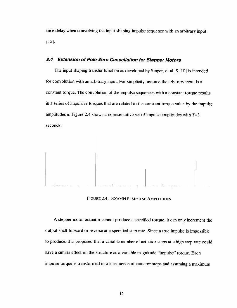
2.4 Extension of Pole-Zero Cancellation for Stepper Motors
The input shaping transfer function as developed by Singer, et al [9, 10] is intended
for convolution with an arbitrary input. For simplicity, assume the arbitrary input is a
constant torque. The convolution of the impulse sequences with a constant torque results
in a series of impulsive torques that are related to the constant torque value by the impulse
amplitudes a. Figure 2.4 shows a representative set of impulse amplitudes with T=3
seconds.
IFIGURE 2.4: EXAMPLE IMPUI,SE AMPLITUDES
A stepper motor actuator cannot produce a specified torque, it can only increment the
output shaft forward or reverse at a specified step r_tte. Since a true impulse is impossible
to produce, it is proposed that a variable number of actuator steps at a high step rate could
have a similar effect on the structure as a variable magnitude "impulse" torque. Each
impulse torque is transformed into a sequence of actuator steps and assuming a maximum
12

step rate is used for all sequences, larger impulse amplitudes result in longer step
sequences, as shown in Figure 2.5.
I
FIGURE 2.5: EXAMPLE IMPULSE AMPLITUDES AND STEP SEQUENCE APPROXIMATIONS
Finally, the step sequences are shifted in time so that each sequence is centered about
the original impulse time as shown in Figure 2.6.
................................................. ................FIGURE 2.6: EXAMPLE TIME -ADJUSTED STEP SEQUENCE APPROXIMATIONS
2.5 Selection and Implementation of Vibration Control Sequences
There are an infinite number of input shaping transfer functions that can be developed.
However, actuator and application-specific constraints will most likely not allow most of
these possible transfer functions and favor some of the remaining over others. To aid in
13

the selection of transfer functions, several guidelines in the form of error calculations are
presented.
2.5.1 Error Calculations
The step sequences produced by the procedure of Section 2.4 do not in general
consist of integer numbers of steps and must be rounded to integer values for
implementation by a stepper motor. The total error produced by rounding the amplitudes
2N+l 2N+ l l/sum Z iErounding = Erounding = a i --round a i
i=1 i=1
is defined as
(2.12
and was one criteria used in the ranking of the many possible input shaper solutions. The
maximum rounding error
max i \Erounding = maX(Erounding, (2.13
within each solution was also calculated. Ranking the solutions in order of increasing error
was developed as an aid in selecting a solution for a simulation run. Concern about the
disparity between the mathematically ideal impulse amplitude and the resulting rounded
number of stepper motor steps assumes the structure is sensitive to the exact number of
steps.
Conversely, if the structure is insensitive to the exact number of steps, then the step
sequences will all have a similar effect on the structt re. It would therefore be desirable
that the vibration control solution require the same l orce or torque on the structure at each
sampling time T. This translates to having all the impulse amplitudes as close in value as
possible. The variation between the normalized impulse amplitudes and an ideal amplitude
14

(which is constant for all 2N+I impulses) was a second criteria used to rank the solutions
and is defined as
2N+I i 2N+I 1
Ev';aUrimation = i_ I Evariatio n _-- 21ai= i=l/ 2N+I
The maximum variation error
max iEvariation = max (Evariation )
(2.14
(2.15
can also be calculated for each solution.
2.5.2 Other Considerations
The values for T must be compatible with the actuator and problem specifications to
generate useful sets of impulse sequences. The actuator is capable of a maximum stepping
rate and therefore a minimum time between steps can be calculated. Therefore, T should
be incremented by this minimum interval throughout a specified range. The range for T
was chosen based on the number of zeros (and therefore the number of step sequences)
that were to be implemented by the input shaper transfer function.
In general, smaller values of T and larger values for N were desirable for several
reasons. Placing N zeros in the shaper transfer function results in 2N+l impulses in the
time domain. As the number of impulses in the solution increases, the number of steps
contained within each step sequence generally decreases, and therefore less time is
required for that sequence. Smaller step sequences should have more of an impulsive
nature in their effect on the structure and can be placed closer together, i.e., the sampling
period T can be smaller. As T decreases, all 2N+ 1 step sequences can be completed in less
15

time and there is more time in the simulation for structural damping to quiet residual
vibrations that could have a significant effect.
16

3 Example Of StructuraIVibration Control
3.1 Overview Of Lewis Spacecraft
The National Aeronautics and Space Agency (NASA) Small Spacecraft Technology
Initiative (SSTI) is intended to demonstrate the viability of new technologies for use in
space. The first pair of these next generation satellites are appropriately named Lewis and
Clark. These satellites feature modular construction and make extensive use of off-the-
shelf hardware. The current SSTI program has formed partnerships between NASA and
two aerospace corporations: TRW is the corporate partner for the Lewis (shown in Figure
3.1 ) and CTA is the partner for the Clark spacecraft.
"_-, _ .......,_. + Z
FIGURE 3.1 : LEWIS SPACECRAFT
17

3.1.1 Lewis Orbital Operations
The Lewis spacecraft [13] will be inserted into a sun-synchronous orbit with a mean
altitude of 283 nautical miles and 97.1 ° inclination. The orbital period will be
approximately 95 minutes and for approximately 63 % of the orbit, Lewis will be in
sunlight. Some of the major operations over the course of a single orbit are illustrated in
Figure 3.2.
While the satellite is in sunlight, there are two primary instruments which will observe
Earth: the Hyper Spectral Imager (HSI) and Linear Etalon Imaging Spectral Array
(LEISA). During the orbital eclipse, the Ultraviolet Cosmic Background Spectrometer
(UCB) will operate to avoid interference from the sun.
The two solar array wings are required to track the sun and maximize power
generation during the sunlit period. The Solar An'a) Drive Assembly (SADA) of the
Maneuver toHSI & Inertial Anti-Sun
LoE_SA _f,___nting
\ Maneuver to
Nadir Pointing
FIGURE 3.2: LEWIS SPACECRAFT ORBITAL OPERATIONS
18

Lewis spacecraft can rotate the solar array wings 360 ° continuously about the Y-axis and
is required to track the sun to within +5 °. For a given orientation of the other two
spacecraft axes with respect to the sun, this specification will assure at least 99.6% of the
maximum solar radiation is available for electrical power generation. The SADA utilizes a
rotary stepper motor which is capable of up to 200 steps or pulses per second (PPS). The
stepper motor actuator imparts impulsive-like torques into the Lewis structure.
The HSI and LEISA instruments have relatively high resolution capabilities and
consequently are sensitive to small amplitude vibrations. The requirements for the UCB
instrument are not critical and it is not necessary for the solar arrays to track the sun
during the 35 minute eclipse. Consequently, this research is limited to the operations and
requirements during the approximately 60 minutes per orbit when the SADA could
potentially incur structural vibrations that reduce the HSI or LEISA data quality. The
range of time these two instruments may require to complete gathering data for an image
and the maximum allowable vibratory motion or jitter of the instrument boresight is given
in Table 3.1.
TABLE 3.1: PAYLOAD INSTRUMENT MISSION REQUIREMENTS
HSI
Minimum Data Acquisition Period 3 sec
Maximum Data Acquisition Period 30 sec
Maximum Allowable Boresight Jitter 10 ktradians, < 250Hz
2 _tradians, > 1500Hz
LEISA
20 sec
50 sec
30 _ radians
19

".2 Physical Description
Table 3.2 summarizes the dimensions, masses, idealized geometry, and the
corresponding moments of inertia of the spacecraft bus and the solar array wings.
TABLE 3.2: LEWIS SPACECRAFT PHYSICAL QUANTITIES
Basic Shape Weight I= lyy
& Dimensions (in) (lbf) (lbf-in-s 2) (lbf-in-s z)
I=(lbf-in-s 2)
Spacecraft Bus Cylinder: 70 x 28 (radius) 797,2
Solar Array Flat Plate: 59 x 138 x 1 26.a.
25.16
3.989
38.78 38.78
0.6167 3.373
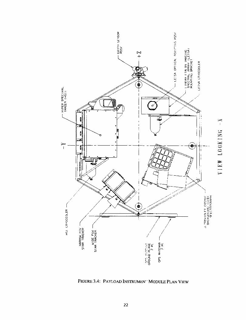
3.1.3 Description Of Payload Instruments Module And Mission Requirements
The payload instruments are attached to the upper payload platform as shown in
Figures 3.4. These items consist of the Hyper Spectral Imager (HSI), Linear Etalon
Imaging Spectral Array (LEISA), Ultraviolet Cosmic Background Spectrograph (UCB),
and both the Wide and Narrow Field of View Star Tracker Assemblies. For each
instrument, there are six possible jitter quantities: a displacement and a rotation
corresponding to each of the three orthogonal Cartvsian coordinates. Displacements have
a negligible effect on the pointing accuracy of instruments in orbit due to the large
distances between the instrument and subject. Therefore, only the three rotations are of
possible concern.
The HSI has a line-of-sight that is fixed relative to the spacecraft and parallel to the Z
axis. The line-of-sight of the LEISA can change within the instrument field-of-regard, but
the field-of-regard is centered about a vector that is parallel to the HSI line-of-sight.
Rotation about the line-of-sight is a secondary conc _rn and so the two important motions
2O

for therotationaljitter arealongthespacecraftX- and Y-axes. The maximum allowable
jitter for these instruments is listed in Table 3.1.
<
FIGURE 3.3: SPACECRAFT DIMENSIONS (INCHES)
21
0
Z
T
+
/
//
/
x
i
=.7Z
FIGURE 3.4: PAYLOAD ]NSTRUMEN'? MODULE PLAN VIEW
22
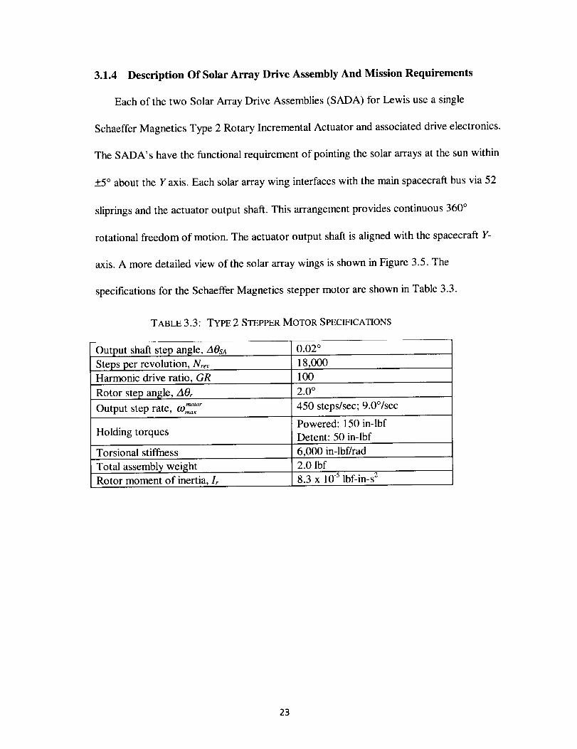
3.1.4 Description Of Solar Array Drive Assembly And Mission Requirements
Each of the two Solar Array Drive Assemblies (SADA) for Lewis use a single
Schaeffer Magnetics Type 2 Rotary Incremental Actuator and associated drive electronics.
The SADA's have the functional requirement of pointing the solar arrays at the sun within
+_5° about the Y axis. Each solar array wing interfaces with the main spacecraft bus via 52
sliprings and the actuator output shaft. This arrangement provides continuous 360 °
rotational freedom of motion. The actuator output shaft is aligned with the spacecraft Y-
axis. A more detailed view of the solar array wings is shown in Figure 3.5. The
specifications for the Schaeffer Magnetics stepper motor are shown in Table 3.3.
TABLE 3.3: TYPE 2 STEPPER MOTOR SPECIFICATIONS
Output shaft step angle, AOsA
Steps per revolution, Nrev
Harmonic drive ratio, GR
Rotor step angle, AOrmotor
Output step rate, 09m_x
0.02 °
18,000
100
2.0 °
450 steps/sec; 9.0°/sec
Powered: 150 in-lbf
Holding torques Detent: 50 in-lbf
Torsional stiffness 6,000 in-lbf/rad
2.0 lbfTotal assembly weight
Rotor moment of inertia, Ir 8.3 x 10 .5 lbf-in-s 2
23

FIGURE3.5: SOLAR ARRAY WING ISOMETRIC VIEW
24

Figures 3.6 and 3.7 illustrate the basic physical dimensions and the main internal
components of the Type 2 actuator. During SADA operation, the stator electromagnets
develop torque on the rotor. The rotor then transfers this torque and resulting angular
motion through the harmonic drive, a gear reduction device. The harmonic drive transfers
the amplified SADA torque to the motor output flange and end load. The end loads for the
Lewis spacecraft SADA's are the solar array panels.
OUTPUT __ STATOR
MEMBER _r_ _r,__.._., £
-- m
.ARMON,O_ [" __' _'_ _-- ROTOR
_---V.,I \ _
BEARINGS
FIGURE 3.6: TYPE 2 STEPPER MOTOR CUT-AWAY VIEW
25

4.00"MOUNTING DIA.
FLANGE --_ , .SMAX
OUTPUT /
FLANGE
3.18"--- DIA
MAX
FIGURE 3.7: TYPE 2 STEPPER MOTOR EXTERNAL Vmw
The Lewis SADA uses a rotational stepper mo :or as an actuator and any desired solar
array orientation corrections must be discretized fo_ implementation by the stepper motor.
During sunlit periods, the power optimal SADA operation would be to continuously move
the solar array at a constant velocity of
09sa - 360 ° = 0-0632_,_ e_,,cki,g To,," , c (3.1
where Torb. is the orbital period, approximately 5700 seconds. Discretizing this quantity
according to the stepper motor specifications result:; in the tracking step rate of
26

oJsa steptracking -- 3.16 (3.2motor --
09tracking AO strap sec
This quantity is about 0.7% of 09mm_°r , the maximum step rate of the actuator listed in
Table 3.3. Experimental investigations by Miller [LaRC, private communication] have
shown step rates up to 100 Hz to be dynamically discrete operations for unloaded
Schaeffer Magnetics Type 1 actuators in the laboratory. However, the Type 2 actuator
employed on Lewis is a larger stepper motor and will have a significantly different
environment and an end load. The motor dynamics are further discussed in Section 3.2.
All simulations for this research were conducted for 10 ° of SADA rotation over a
total time of 160 seconds. These parameters were chosen based on two requirements.
First, the normal to the solar array panels is allowed to vary up to 5 ° about the Y axes
from the sun vector, resulting in at most a 0.4% decrease from the maximum possible
incident solar radiation. This allows a maximum rotational motion at one time of 10 °, if
the solar arrays begin with a 5 ° bias. Second, this amount of rotation for the solar arrays is
required over an interval of time dictated by the orbital period and is
10 °-- 158.3 seconds (3.3
(-1")tracking
which was then rounded up to 160 seconds.
3.1.5 Angular Momentum Calculations
A single finite element model (FEM) was used to simulate the spacecraft structure.
This model had a fixed orientation of the solar arrays relative to the spacecraft bus and did
not allow the rotation of the solar array panels to be simulated. Therefore, the simulated
27

SADA torqueactsasanexternaltorqueon theFEVIat thenodescorrespondingto the
SADA's andisnot representedbyequalandoppo_,iteinternaltorques.Theangular
momentumof thesystemisnot conserved since the SADA output acts as an external
torque. To provide a basic check on the simulation results the following calculations are
performed.
By rotating both solar arrays at the solar track ng velocity, the simulated SADA
J
torque should increase the angular momentum of the system by the quantity
--SA SA = 1.36x10⁻³ lbf .in .sec130. O)tracking (3.4
Dividing this angular momentum increase by the combined inertia of the spacecraft bus
and the solar arrays yields the average angular velocity of the spacecraft expected from the
CSRS simulation as
,,/,. 0_ 5 radiaasto,,ack,,g = 3.4 x 1 (3.5
sec
A simulated 10 ° rotation of the solar array panels will maintain this average velocity for
158.3 seconds and cause a total spacecraft rotation of
A t_s/" = 5.4×10 -3 radiansV simulation (3.6
This quantity is then used as a basic check on the wtrious stepper motor command
sequences. Since each sequence should simulate a 10 ° solar array rotation, the total
:/c
spacecraft rotation should approximately equal A0. imu_,eon•
28

3.2 Lewis Spacecraft Dynamic Model
Several different analytical tools were used to complete this research. A model of the
Lewis spacecraft structural dynamics was a core element, and it was fundamental to
producing the final results simulating the jitter experienced by the payload instruments. A
separate dynamic model of the Schaeffer Magnetics Type 2 actuator employed within the
Solar Array Drive Assembly (SADA) was used to develop the torque time profiles of the
SADA operations. These two components were then incorporated into one computer
based simulation through the use of the PLATSIM [4] analysis package.
3.2.1 Structural Model
A NASTRAN finite element model was used to develop a modal model of the
spacecraft structural dynamics. The finite element model (FEM) eigensolution identified
the flexible body modes and the corresponding lowest 163 natural frequencies are listed in
Appendix B. The modal damping ratio was modeled as 0.2% for all modes. The mass-
normalized modeshapes at the nodes corresponding to the HSI and LEISA instruments
and the two SADA's were available to the author. The modeshape information was not
included for space considerations.
3.2.2 PLATSlM Linear Analysis Software
PLATSIM [4] is a NASA Langley Research Center developed software package that
incorporates the spacecraft modal model, ACS description, and the disturbance models
into one dynamic simulation. Various disturbance scenarios can be constructed and used
as input to the modal model. During a time domain simulation, these scenarios are input to
the modal model at the specific node(s) associated with the disturbance source. The
29

responseof specificnodescanbeselectedandtheirresponsetrackedduring the
simulation. Displacement, rate, or acceleration data can be chosen as the output for each
node and jitter analysis can be conducted.
3.2.3 Stepper Motor Model
Farley modified a dynamic model of a Schaeffer Magnetics Type 1 actuator [3] to
represent a Type 2 actuator for the author [private communication]. Additional data for
the Lewis spacecraft application was determined [13] and used to create various torque
time profiles of the motor output flange.
The four degree of freedom (DOF) electromechanical dynamic model developed by
Farley is shown in Figure 3.8. The inertia, damping, and stiffness characteristics of the
spacecraft, motor rotor, harmonic drive gear reduclion, end load and their connecting
elements are included. The coulomb friction acting an the harmonic drive gear reduction
inside the stepper motor (TFint) and acting on the output flange (TFext) are also included.
The data used in the motor simulation to describe the model is listed in Tables 3.4 and 3.5
The static, back EMF, and transient currents in the stepper motor electrical system
can be calculated from the motor model. These cunents superpose within the
electromagnets to develop torque on the rotor. The model requires the permanent magnet
or detent torque maximum amplitude, motor electrizal constant, resistance of each phase
separately, series resistance of all 3 phases, inducta:tce of each phase, and applied voltage.
The motor was treated as having a constant voltage source and the limiting current (the
largest current that can be drawn by the motor) wa_, therefore defined.
30

--HARMONIC DRIVE STIFFNESSGEAR REDUFTIBN _.
. ,q _ GR \ -HARMONIC DRIVE VI,>COU,L, DAMPING_ U1 . "".., ,---OUTPUT FLANGE INERTIA
% ',. , I ), ,_] , , ,,.+e:, r_4. ,, / , _. _ /_EXTERNAL COULOMB FRICTION TFe×'t
,4 X__/' \ Ft%, .... jT_
/, \, _ .......
I / _INTERJ}AL COLILOM_ FRICTION '\ L,_L_V_OLAR_'RAYiNERTIA\ J2/ /_ TFIr.t; , LOAD ,?,TIFFNEoS
#\, /; .../## 'L-LOAD \."[SCOU3 ]]ANPING
/ _'-LL_-_NOTOR ROTOR INERTIA
LNOTOR RBTOP, VISCOUS DAMPING
L-SPACECRAFT/MOTOR HOUSING/STATOR INERTIA
FIGURE 3.8: FOUR-DOF STEPPER MOTOR MODEL DIAGRAM
TABLE 3.4: STEPPER MOTOR MODEL MECHANICAL SPECIFICATIONS
Motor Rotor Inertia, J1
Spacecraft Inertia, J2
Output Flange Inertia, J3
Load / Solar Array Inertia, J4
Harmonic Drive Torsional Stiffness, K23
Load Torsional Stiffness, K34
Rotor Viscous Damping, C12
Harmonic Drive Damping Ratio, C23
Flexible Load Damping Ratio, C34
External Coulomb Friction, TFext
Internal Coulomb Friction, TFint
Gear Reduction Ratio, GR
Output Step Size
9.38x10 -6 Kg-m 2
4.38 Kg-m 2
0.03 Kg-m 2
0.0697 Kg-m 2
677.9 N-M/rad
50 N-M/rad
0.0 N-m/rad-sec
0.1
0.02
0.268 N-m
0.117 N-m (Rotor Break-away Friction)
0.003 radians (Dahl Friction Factor)
100:1
2 degrees
31

TABLE 3.5: STEPPER MOTOR MODEL E;_ECTRICAL SPECIFICATIONS
Applied VoltageCurrent Limit
Phase Inductance
Series Resistance (all phases)
Phase Resistance
Motor Constant
Detent TorqueMaximum Pulse Width
Minimum Dead Time Between Pulses
12 _olts
0.5 amps
0.003 Henrys0.35 Ohms
12 Ohms
0.169477 N-m/Amp0.056492 N-m
0.035 seconds
0.01105 seconds
Different types of stepping sequences can be simulated within the model: a constant
step rate, or a linear ramping or staircase ramping of the step rate. Only a constant 200
steps or pulses per second (PPS) step rate was used for this research, but it is common
practice to ramp up the motor step rate in various ways to more smoothly accelerate the
load. These other methods would be of possible interest in further studies of vibration
control using stepper motors. For all step rate options, the motor model requires
information about the maximum pulse width and minimum dead time or spacing between
pulses, as illustrated in Figure 3.9 and listed in Table 3.5.
MINIMUM PULSE
PULSE _IITH
FIGURE 3.9: MOTOR STEPPING OPF RATION PARAMETERS
32

3.3 Determination of Target Modes
The NASTRAN analysis of the fmite element model of Lewis returned a mass-
normalized eigenvalue solution and the 163 lowest frequency flexible-body modes were
then identified. A frequency response function analysis was used to determine the modes
that had the strongest coupling between the two SADA input nodes and the two payload
instrument output nodes.
3.3.1 Finite Element Analysis Results
Modeshapes are ratios of motions between all of the nodes within a finite element
model and only the relative magnitude of a particular value is important. Most of the low
frequency modes involve relatively large motions of the solar arrays compared to the
deflection of the rest of the structure, and this is not surprising due to their large size and
flexibility. The modeshape values, however, do not directly indicate the quantitative
relationship between SADA input and the resulting payload instrument motion.
The natural frequencies identified range from 0.3 Hz to 149.5 Hz with 13 modes
having a resonant frequency below 10 Hz. The damping ratio for all modes was modeled
as 0.2% and lower frequency modes would dissipate energy more slowly than high
frequency modes. Therefore, the low frequency modes would affect the jitter at the
payload instruments more than higher frequency modes during a quiescent period without
SADA input.
The stepper motor input is simulated at 200 PPS and would be expected to excite
high frequency modes. High frequency modes would therefore possibly affect the jitter at
the payload instruments more than lower frequency modes during active periods with
33

SADA input.Selectingthetargetmodesfor pole-zerocancellationwill requireamore
objective FRF analysis.
3.3.2 Frequency Response Function
The frequency response function (FRF) quantitatively defines the relationship between
a pair of input and output locations within a structure over a range of frequencies. The
coordinate direction of each location must be defined as well. For example, an input could
be at one of the SADA nodes with a torque in the Y direction, and an output could be the
rotation about the X-axis of the HSI node.
For a modal, two degree of freedom system, the FRF reduces to
/ mr (3.7Ho(o)):_((D_rr=l -- 092) + j2_.tOnr09
where there are N modes to be included. The gh mode has a natural frequency akr,
damping ratio (r, modal mass mr, and corresponding modeshape coefficients _ir and _jr
(for input node i and output node j). Ho(_ ) is a cort_plex number and typically is shown on
a magnitude and phase plot. To evaluate the importance of each mode to the input-output
relationship, only the magnitude information is of ccmcern.
Normally, the response for all the N modes is s Jmmed as shown in Equation 3.7. The
modes can be ranked in contribution to the magnitu de of the input-output relationship by
calculating the frequency response function for eact mode at its natural frequency. This
results in the purely imaginary quantity
34

= /mr ts.s
Each mode therefore contributes a specific magnitude response at the output location
to a unit input. These 163 different values are then sorted and used to identify the most
important modes in causing the output response. Both Equations 3.7 and 3.8 were used
for a total of eight different input output pairs: both SADA's as inputs and the HSI X-
rotation, LEISA X-rotation, HSI Y-rotation, and LEISA Y-rotation as outputs.
3.3.3 Modal Input-Output Analysis
The two different SADA nodes were denoted as SADA #1 and SADA #2 for clarity.
All simulations operated both solar array drives in tandem, using the same vibration
control solution to determine the step sequences. Therefore the SADA's are handled
separately only during the FRF analysis. The FRF analysis was performed for all eight
input-output pairs: two SADA's with torque about the Y-axis as inputs and the HSI and
LEISA rotations about the X- and Y-axes as outputs.
Figure 3.10 shows the FRF for the input-output pair SADA #1 (Y-rotation) - HSI (X-
rotation). The lower frequencies have the largest magnitude response, but there is a broad
band of increased coupling from about 65 to 130 Hz. Specifically, the two highest peaks
occur under 5 Hz and there are other sizable responses at about 65 Hz, 85 Hz, and 115
Hz.
35

o)
c-C_
U_rr"
U_
o
9
8
oI
>,-
c_
O9
I I I f I I I
J
J
ff_
.__2-
S
L3
O
O
O
NT
O
OCd
0 0 0 0 0 0 _ 0 00 _ 0 _ _ 0 _ 0
I I I
0s_qd
E
E0
v
I
0
I
a
0
r
, _il_i.1 i, , I.,,BB, ,
0 0 0 0
epnl!ldmV
0
r
0
0
O
0 0
FIGURE 3.10: SADA #1 Y-ROTATION (INPUT) -- HSI X-ROTATION (OUTPUT) FRF
36

Useof Equation3.8rankedeachmodein its importancewith respectto this input-
outputpair.A semilogplot of therankedmodesis showninFigure3.11.Thetwo highest
decadesof theplot contain10modes,with theother153modesdecreasingto eight orders
of magnitudeless.
-o 1
e-cn 1m
I.Lne 1tl
1
1.E-04
1.E-05
1.E-06
•E-O7
•E-08
•E-09
.E-IO
.E-11
.E-121.E-13
1.E-141 19 37 55 73 91 109 127 145 163
Modal Rank
FIGURE 3.11 : SADA #1 Y-ROTATION - HSI X-ROTATION RANKED MODES ( 1)
The ten highest magnitude modes are plotted linearly in Figure 3.12. This plot clearly
shows the importance of each mode in the magnitude of the output response to a unit
input. The contribution from mode #4 is approximately six times that of the next two,
modes #3 and #8. Appendix C contains the FRF analysis plots for the remaining seven
input-output pairs.
37

SADA 1 (Y-rotation) - HSI (X-rotation) Modal FRF Amplitudes
7.E-05
6.E-05
5.E-05o
1.E-05
FIGURE 3.12:
137
SADA #1 Y-ROTATION - HSI ,_'-ROTATION RANKED MODES (2)
3.3.4 Selection of Target Modes
Table 3.6 and Figure 3.13 summarize the result s of half of the FRF analysis by
presenting the ten modes that provide the strongest input-output correlation in order of
payload instrument X-rotation magnitude. The threc largest contributors to both the HSI
and LEISA X-rotations for both SADA inputs are modes #3, #4, and #8 although the
modes are varied in ranking between the two SAD,_,'s. The other modes common to the
four input-output pairs are #2 and #7. Of the remaking modes, #11 is ranked fourth for
SADA #2 and the other modes are of decreasing importance. Therefore modes #2, #3, #4,
#7, and #8 and possibly #11 would be recommended as target modes for input shaping to
reduce payload instrument X-rotation.
38

TABLE 3.6: RANKED MODES FOR PAYLOAD INSTRUMENT X-ROTATIONS
SADA #1 Input Mode Number
HSI Output 4 3 8 7 2 79 118 53 132 137
LEISA Output 4 3 8 7 2 118 53 137 117 109
SADA #2 Input
HSI Output 3 8 4 11 7 2 68 69 53 118
LEISA Output 3 8 4 11 7 2 118 119 53 82
DSADA #1 - HSlDSADA #1 - LEISA
R SADA #2 - HSl
[D SADA #2 - LEISA
0.E+00 .
1
FIGURE 3.13:
2 3 4 5 6 7 8 9 10
Mode Rank
PAYLOAD INSTRUMENT X-ROTATION FRF MAGNITUDES
Table 3.7 summarizes the results of the second half of the FRF analysis by listing the
10 modes that provide the strongest input-output correlation in order of payload
instrument Y-rotation magnitude. The two largest contributors to both the HSI and LEISA
X-rotations for both SADA inputs are modes #3 and #4. The magnitude of the input-
output correlation for both of these modes is much greater than for any of the other
39

modes,asshownbyFigure3.14.Theonly othermodescommonto thefour input-output
pairsare#40,#1, and#7. Of theremainingmodes,#12and#11 arerankedfourthfor
SADA #1andSADA #2 respectively,andtheremainderareof decreasingimportance.
Modes#3and#4 arethemostimportantandmodes#1,#7,#11,#12,and#40areof
secondaryimportanceastargetmodesfor input shapingto reducepayloadinstrumentY-
rotation.
TABLE 3.7:
SADA #I Input
RANKED MODES FOR PAYLOAD INSTRUMENT Y-ROTATIONS
Mode Number
HSI Output
LEISA Output
4 3 12 40 1 7 117 97 109 79
4 3 12 40 1 7 117 97 79 109
3 4 11 40 68 69 1 7 43 8
3 4 11 40 68 69 1 7 43 8
SADA #2 Input
HSIOutput
LEISAOutput
40

3.5E-03
3.0E-03
2.5E-03
w
_ 2.0E-03
_ 1.5E-03
o
1.0E-03
5.0E-04 -_
O.OE+O0
1 2 3 4 5 6 7 8 9 10
Mode Rank
r'l SADA #1 - HSI I
[3 SADA #1 - LEISA I
[] SADA #2 - HSI
E] SADA #2 - LEISA
FIGURE 3.14: PAYLOAD INSTRUMENT Y-ROTATION ERE MAGNITUDES
41
4 Simulations And Results
The analysis technique used to evaluate the structural vibrations due to the SADA
torque inputs is presented and then the structural responses and calculated vibration levels
for the two baseline simulations are discussed. The application to the Lewis spacecraft of
the pole-zero cancellation technique is introduced and the results from three vibration
control simulations are included. These examples illustrate the vibration control effects of
pole-zero cancellation and a method for increasing .;haper robustness to errors in system
identification.
4.1 Jitter Analysis Method
Motion of the solar array panels must be acconlplished without exciting structural
modes beyond acceptable jitter for the various payloads onboard. Jitter is usually defined
as the absolute value of the peak-to-peak change in the displacement or rotation of a
particular point on the spacecraft during a period of time called a jitter window. As an
example, a jitter requirement might be "10 ktradians / 1 sec" which means a maximum of
10 l.tradians of rotation is allowable over any one second period of time.
When the period of a sinusoidal or other perioc ic vibration is less than the jitter
window, the vibration will complete at least one ful cycle during the jitter window. The
resulting jitter would then equal the peak-to-peak a:nplitude of the vibration. When the
jitter window is less time than the vibration period, -he jitter also depends on the phase of
the vibration in the jitter window as well as the vibration amplitude. Therefore, careful
42

selection of jitter windows can restrict the contributions of vibrations below the jitter
cutoff frequency, which is defined here as the reciprocal of the jitter window.
The total time the jitter is of concern can be much longer than the jitter window. The
largest jitter value that occurs during the total time of interest is known as the maximum
jitter. Continuing the previous example, let the 10 I.tradians / 1 sec jitter requirement be
prescribed for total time of interest of 3 seconds. In Figure 4.1, two different sinusoidal
vibrations are shown and a one second long jitter window is specified. Since the 3 Hz
vibration completes several cycles during the jitter window, it has a jitter that is equal to
the peak-to-peak amplitude (2.5 ktradians in this example) and is constant for the total
time of interest. The displacement due to the 0.5 Hz vibration during the jitter window
indicated is 2 _tradians. However, the lower frequency vibration has a longer period than
the jitter window (i.e., the vibration frequency is below the jitter cutoff frequency), and
therefore the maximum displacement within the jitter window also depends on the phase
of the vibration.
43

0 0.5 1 1.5 2 2.5 3
Time, IleCOrldll
FIGURE 4.1" JITTER ANALY_',IS EXAMPLE ( l )
2.5
1.5
m
0.5
!- 0
e-o
_o -0.5
-1.5
-2
-2.5
0.5 Hz
•................... _ vibration
Js:
/
vibration
y?
7:/
%
\, I,_ Jitter
,,.< _ ,+ Windo
0.5 1 1.5 2 2.5
Time, liecol_,d II
FIGURE 4.2: JITTER ANALY_ IS EXAMPLE (2)
44

For aonesecondjitter windowfrom 1.5to 2.5secondsthedisplacementfor the0.5
Hz vibrationwoulddoubleto 4 _radiansasshownin Figure4.2.If thejitter windowis
"slid" in thismanneralongthetotal timeof interestthemaximumjitter for all possible
jitter windowscanbefound.Morecomputationallyefficientmeansof calculatingjitter [5]
wereusedfor thisresearchbut theresultis thesame.Since4 txradiansis themaximum
jitter value,theseexamplevibrationswouldsatisfythe 10I.tradians/ 1 second jitter
requirement for the entire time shown. Only the maximum rotation over all possible jitter
windows is of interest, and so the term jitter alone will be used to refer to the maximum
jitter. Jitter analysis of this nature will be used to determine the effectiveness of the
vibration reduction.
4.1.1 Selection of Jitter Windows and Analysis Start Time
Use of different length jitter windows can better reveal the vibration due to a
particular frequency range of modes. The shorter length windows will not allow lower
frequency vibrations to complete a full cycle within the window and therefore the
measured jitter due to lower frequency modes will be diminished. Table 4.1 details the
jitter windows used and the corresponding cutoff frequency, and lists the modes that are
above the cutoff frequency and therefore able to contribute fully within that jitter window.
The modal frequencies as determined by the FEM eigensolution are listed in Appendix B.
TABLE 4.1 : EFFECT OF JITFER WINDOWS ON MODAL CONTRIBUTIONS
Jitter Window, seconds 0.05 0.1 0.2 0.5 1.0 3.5
Cutoff Frequency, Hz 20 10 5 2 1 0.286
Fully Included Modes 23-163 15-163 10-163 8-163 3-163 1-163
45

Thecutoff frequencyisnot anabsolutedemarcation,however.By strict calculation,
the0.2 secondwindowdoesnotallowthefull conlributionof mode#9, whichhasa
naturalfrequencyof 4.97Hz. However,99.4%of onecycleat thatfrequencywill fit in the
0.2 secondjitter window andsomode#9cannotbeconsideredexcludedfrom
contributingsignificantlyto jitter in thatwindow.Thelongestjitter window(3.5seconds),
allowsall thestructuralmodescontainedwithin thefiniteelementmodelof Lewis to fully
contribute.Jitter windowslongerthanthisperiodof timewill only showtheadditional
effectsof rigid bodymotions,whichwill notbe reducedbythisvibrationcontrol
technique.
Jitter analysiswasconductedinitiallyto find themaximumjitter over theentire160
secondsimulation.The "starttime" of theanalysiswould thereforebet=0. This starting
time was increased by 0.5 seconds for each subsequent analysis, up to t=156.5 seconds.
Increasing the jitter analysis start times allowed trallsient responses from earlier SADA
disturbances to dissipate and not be included in the later analyses. Since the jitter tended to
decrease over the simulation time, this allowed a determination of when the jitter levels
were acceptable for the remainder of the simulatior.
4.2 Baseline Simulations And Jitter Analysis Results
Torque time profiles were used to simulate the SADA outputs resulting from the five
stepper command sequences presented in this research. Jitter analysis using six different
jitter windows was conducted on the resulting X- a:ld Y-rotations of the two FEM nodes
corresponding to the HSI and LEISA payload instraments. These 24 different analyses
46

were conducted over the course of the simulation and used to determine the relative
effectiveness of the vibration control method in comparison to baseline results.
4.2.1 Constant Step Rate Simulation
The torque variation of a single step of the SADA rotary actuator is shown in Figure
4.3. The duration of a single step is about 1/40 th of a second from beginning to end and
therefore up to about a 40 Hz step rate would be expected to consist of entirely discrete
operations. This is a reasonable result given that a smaller rotary stepper motor with
lighter end-loading conditions was found by Jim Miller of NASA Langley Research Center
[private communication] to have discrete steps up to 100 Hz. Cascading these steps at the
prescribed step rate of approximately 3.16 steps or pulses per second (PPS) results in the
Constant Step Rate Sequence (CSRS) torque input, a portion of which is shown in Figure
4.4. This plot illustrates the short time length and impulsive nature of the individual steps.
47

|t-
d-.1
EO
I-
2
0
-1
-2
-3
-4 4ii
-5 i _ _ I I I I I t I
0 0.005 0.01 0.015 0.02
Time, seconds
FIGURE 4.3: SINGLE STEP TORQUE TIME PROFILE
r i 1 i T I- r T I
0.5
0
I
-0.5'-,l
OI.---
-1
-1.5
-2 _-0 0.2 0.4 0.6 0.8 1
Time, sec
J
1.2 1.4 1.6 1.8 2
FIGURE4.4: CSRS TORQUE TIM:. PROFILE, 3.16 PPS
48

The X- and Y-rotations of the HSI instrument are shown in Figures 4.5 and 4.6. These
figures show the total response (combined rigid and flexible body terms) and the flexible
body response alone. The rigid body Y-rotation of the HSI instrument was approximately
5,350 laradians, close to the quantity predicted by Equation 3.6. The rigid body X- and Z-
rotations are approximately -102 and -13.5 gradians respectively, and this indicates that
the simulated spacecraft structure transfers some energy between the coordinate directions
via non-zero off-diagonal terms in the inertia matrix.
csrs HSI X-Rotation ResponseI I I I t I I
-12 I 1 = J I i0 20 40 60 80 100 120 140 160
csrs HSI X-Rotation Flexible-Body ResponseI I I I I I I
(/}t--
-o
o
0t--
O°_
t_o
n-
-50 20
FIGURE 4.5:
I I I I I I
40 60 80 100 120 140
Time, seconds
HSI X-ROTATION RESPONSE TO CSRS TORQUE INPUT
160
49

x 10-3 csrs HSI Y-Rotation Response6 I I I I 1 ] I
O9t- 5
-o 4
o.o_ 3E. 2
t-O
+5rr 0
-1 I I I L I I I0 20 40 60 80 100 120 140 160
x 10-s1.5
1
0.5
0
-0.5
-1
-1.50
csrs HSI Y-Rotation Flexible-Body ResponseI I I I I I I
¢/}¢-
"1o
oo
E
¢-.2
on"
I I I I I I I
20 40 60 80 100 120 140
Time, seconds
160
FIGURE 4.6: HSI Y-ROTATION RESPONSE TO CSRS TORQUE INPUT
For both instruments, the jitter response to the CSRS torque input are nearly constant
values for all analysis start times. Within the simulation, the HSI and LEISA nodes achieve
a steady state response almost immediately to the r,.'petitive CSRS torque input. Table 4.2
summarizes the average jitter levels for the six jitter windows used.
The Y-rotation jitter levels are clearly not acceptable and have significant input from
the higher frequency modes (i.e., the jitter levels orly increase slightly as the jitter window
is lengthened from 0.05 seconds to 3.5 seconds). The X-rotation is much less, and is due
50

to the structural transfer of rotational energy since the input torque is acting about the Y-
axis only.
TABLE 4.2: CSRS JrlTER ANALYSIS RESULTS
Jitter HSI LEISA HSI LEISA
Windows X-rotation X-rotation Y-rotation Y-rotation
in seconds
0.05
0.1
0.2
0.5
1
3.5
Jitter, ttradians
% of Jitter Limit
Jitter, l.tradians
% of Jitter Limit
Jitter, ].tradians
% of Jitter Limit
Jitter, tzradians
% of Jitter Limit
Jitter, [zradians
% of Jitter Limit
Jitter, tlradians
% of Jitter Limit
7.20 5.91 16.96 51.95
72.0% 19.7% 169.6% 173.2%
7.20 5.91 16.99 51.95
72.0% 19.7% 169.9% 173.2%
7.20 5.91 17.56 51.95
72.0% 19.7% 175.6% 173.2%
7.79 5.97 18.87 54.31
77.9% 19.9% 188.7% 181.0%
7.79 5.99 19.01 54.32
77.9% 20.0% 190.1% 181.1%
7.80 6.00 19.07 54.43
78.0% 190.7%20.0% 181.4%
4.2.2 Minimum Actuation Time Simulation
A single actuator sequence consisting of 500 consecutive steps at the maximum rate
of 200 pulses per second (PPS) was simulated. The first 0.5 seconds of the 200 PPS
torque output is shown in Figure 4.7. This achieves the required 10 ° of rotation in a
minimum time of 2.5 seconds and would allow a maximum amount of time for structural
damping to dissipate the vibrational energy. The stepper motor torque output at high step
rates loses its distinct step characteristics. The response of the HSI to the MATS torque
input is shown in Figures 4.8 and 4.9.
51

.Q
I
EO
F-
0
--1
--2
--30
I I I I I I I I
0.05 0.1 0.15 0.2 0.25 0.3 0.35 0.4Time, sec
FIGURE 4.7: MATS TORQUE TIME PROFILE, 200 PPS
I
0.45 0.5
52

x10-5 mats HSI X-Rotation Response5 ! I I I I I I
c
0
Po
"_ -5
t-O4--'
-10o
rr
-150
I I I I I
20 40 60 80 100
I I
120 140 160
x 10 -54
mats HSI X-Rotation Flexible-Body ResponseI I I I i 1 l
u)ca_
2
oo
"_ 0C
o.I
"_-2'5rr"
-4 i i i i t i i0 20 40 60 80 100 120 140 160
Time, seconds
HSI X-ROTATION RESPONSE TO MATS TORQUE INPUTFIGURE 4.8:
The rigid body Y-rotation for the spacecraft is approximately 5,350 l.tradians, agreeing
with the response from the CSRS input. After the SADA input is complete at t=2.5
seconds, the spacecraft structure was allowed to settle until t=160 seconds. The HSI Y-
rotation response during the settling period consists of a superposition of decaying
sinusoids from the simulated structural modes. Jitter analysis was conducted as stated
previously over the entire simulation time.
53

x 10-3 mats HSI Y-Rotation Response6
(/)¢-
O
E
t-O
m
On-
5
4
3
2
1
0
-10
I I I I I T
i I I I I 1 I
20 40 60 80 100 120 140 160
x 10 -410
mats HSI Y-Rotation Flexible-Body Response+ I l I I I I
I I I I I I I
20 40 60 80 100 120 140 160Time, seconds
HS[Y-ROTATIONRESPONSETOMATS TORQUE INPUTFIGURE 4.9:
The jitter analysis results for both the CSRS an] MATS simulations are summarized
in Figures 4.10 through 4.13, and show the jitter va3ues as percentages of the instrument
jitter limits. Jitter analyses of the MATS simulation "esponse with a start time of t=0 had
the largest values. The jitter levels steadily decreased as the analysis start time progressed
and the last jitter analyses, with a start time of t=-15{,.5 seconds, had the minimum value.
54

--I
.-j
'5
8
1000% ...........................................................................................................................................................................i
100%
10%
1%
Jitter Windows, seconds
FIGURE 4.10: HSI X-ROTATION BASELINE JITTER LEVELS
.J
'54.,I¢.
8t,i
[] CSRS
[] MATS Maximum
• MATS Mean• MATS Minimum
Jitter Windows, seconds
FIGURE 4. l l : LEISA X-ROTATION BASELINE JITTER LEVELS
55

_ 1OOOOO%-I
10000%
"_ 1000%"6c
8 100%
,_ 10%
CSFIS
Mu_TS F_.,4mum
_TS Mean
MATS Minimum
FIGURE 4.12:
L05
, i9.60
166.0
5.7%h
3.7°/0
0.2 _"0.5 1 I' 3.5
90 K).70
,.0 :'24.0
i% 171.0
;% 3.5%
Jitter Windows, seconds
HSI Y-ROTATION BASELINE JITTER LEVELS
i_ 10000%-I
G)
15
0L_
0
1000%
100%
10%
[] CSRS 1
[] MATS Maximum 1;
[] MATS Mean 1
• MATS Minimum ;
B-_m
m.05
L18%
17.0%
1.6°/o
.9%
,- #it
Jitter Windows, seconds
FIGURE 4.13: LEISA Y-ROTATION E ASELINE JITTER LEVELS
Examination of the MATS simulation response reveals that the average and minimum
X-rotations are below the desired jitter limits, but the corresponding Y-rotations generally
exceed the limits. The HSI minimum Y-rotation jittcr values are above the instrument jitter
56

limit for the5longerjitter windows,with onlythe0.05secondwindow havingan
acceptableminimumjitter value(68.7%of thejitter limit, seeFigure4.12).Structural
damping(modeledas0.2%for all modes)decreasedtheminimumLEISA Y-rotation jitter
for the 0.5, 1.0 and 3.5 second windows to 124.4% of the instrument jitter limit (see
Figure 4.13). These results illustrate that with a lightly damped system the structural
modes can cause sustained vibratory motion that could reduce the data quality from the
payload instruments and a more advanced command sequence could be employed to
directly address this concern.
4.3 Shaped Input Simulations and Results
The implementation of the z-plane pole-zero cancellation theory for the Lewis
spacecraft SADA is presented. To aid in the selection of input shaper solutions, additional
calculations using four different criteria are performed. These calculations rank the many
possible sets of stepper motor sequences produced by the vibration control theory. The
proposed solutions were then transformed into equivalent SADA torque time profiles and
the Lewis spacecraft response was simulated using the model introduced in Section 3.
Jitter analysis was then performed to evaluate the performance of each sequence in
reducing vibration. The results from three of these simulations are presented in Sections
4.3.
The target modes were selected as discussed in Section 3.3. The corresponding target
poles were calculated from the modal information according to Equation 2.4 and the
discrete time transfer function was constructed. This transfer function was transformed to
the Laplace s-domain and the numerator coefficients were extracted. These coefficients
57

aretheimpulseamplitudesof Equation2.11,andsolutionswith anynegativeimpulses
wereremoved.This is notessential,but removingsolutionswith negativeimpulses
ensuredthat theSADA wouldalwaysmovethesolararraysin thedesireddirection.Other
researchershaveinvestigatedthe useof negativeimpulsesto shortenthetimeintervalT
between impulses [8] but this was not investigated for the Lewis spacecraft. The impulse
amplitudes of the remaining solutions were normalized to sum to one. The four ranking
criteria of Equations 2.12 through 2.15 were calculated and based on these rankings, one
or more solutions were selected and used with the PLATSIM Lewis simulation.
The stepper sequence(s) defined by a given input shaper solution was then used to
construct an SADA torque time profile. This torque profile contained the desired number
of steps in each sequence and had each sequence spaced in time at a center-to-center
distance equal to T as shown in Figure 2.6. The simulated SADA torque was applied to
the SADA nodes within an open-loop simulation (to remove any effects from the Lewis
spacecraft ACS) and the resulting jitter levels of the HSI and LEISA payload instruments
examined to evaluate the vibration reduction.
The results for all eight input-output pairs must be considered in the selection of
target modes for the input shaper, since the one sh_ per is to attempt to reduce the four
output vibrations. The X-rotations from the constant step rate and single sequence
simulations were below the jitter limits for all jitter windows, and so it was desired to
maintain that performance. At the same time, the simulated Y-rotations were up to 1.5
times the jitter limits and so that performance had t a be improved. Comparison of the FRF
analysis plots show that a torque input about the Y-axis by either of the SADA's has a
58

muchgreaterimpacton theY-rotation of the payload instruments than on the X-rotation
of that node. Therefore, the controllability of the Y-rotations by the SADA torque is
greater.
4.3.1 Vibration Control Sequence #1
Table 4.3 shows the information that fully describes Vibration Control Sequence #1
(VCS #1) as implemented for the Lewis spacecraft. The Target Modes are the modes
selected using the FRF analysis of Section 3.3. The Target Robustness is the total number
of zeros that are placed over the corresponding system poles by the shaper transfer
function. The Impulse Amplitudes listed are the normalized values, and the Step Time is
the time at which each step sequence begins, adjusted as explained in Section 2.4. The
system poles corresponding to the eight target modes are plotted in the z-plane in Figure
4.14, and the shaper zeros are placed exactly over the system poles in this command
sequence. The first 30 seconds of the SADA torque for VCS #1 is shown in Figure 4.15,
with the torque being zero from t=30 to t=160 seconds.
59

TABLE 4.3: VIBRATION CONTROL SEQUENCE #1 DATA
Target Modes
Target Robustness
Total # Impulses
Sampling Time, T
Step Rate
#2 #3 #4 #7 #8 #11 #12 #40
1 2 2 1 2 1 1 1
23
1.14 seconds
200 PPS
#Impulse #12
3
4
56
7
8
9
10
11
121314
15
1617
1819
20
21
22
23
Totals
Impulse Amplitudes
0.023073
0.03148
0.0361540.08806
0.0517580.040324
0.094088
0.0128030.047849
0.1137210.037566
0.093490.100759
0.0221690.050666
0.0363880.008973
0.0324920.029042
0.0192620.017665
0.0097630.002455
1.00
Steps
1216
18
4426
2047
624
5719
4750
1125
184
1615
109
51
Impulse Time, seconds
5O0
01.14
2.28
3.424.56
5.76.84
7.989.12
10.2611.4
12.54
13.6814.8215.96
17.1
18.2419.3820.52
21.66
22.823.94
25.08
Step Time, seconds0
1.1252.255
3.325
4.5055.655
6.72257.96
9.0510.1025
11.3325
12.397513.52514.7575
15.857517.01
18.1819.285
20.4225
21.5722.707523.8525
24.9975
60

X
\\
\
/
FIGURE 4.14: SYSTEM POLES IN THE Z-PLANE (T= 1.14 SECONDS)
61

t-_
It---o_
-1
Ol-
4
-2
-4
-6
I I I I I -
-8-L L I I i
0 5 10 15 20 25Time, seconds
FIGURE 4.15: SADA TORQUE TIME PROFILE FOR VCS #1
The HSI X- and Y-rotations resulting from the VCS #1 input torque are depicted in
Figures 4.16 and 4.17. The LEISA response was n_arly identical within the scale of the
graph. The total rigid body Y-rotation of the spacecraft agrees quite closely with the
prediction of Equation 3.6 and is approximately 5,350 _tradians.
62

x 10 -s5
vcsl HSI X-Rotation ResponseI I 1 I I I I
20
I I I I I I
40 60 80 100 120 140 160
x 10 -s vcsl HSI X-Rotation Flexible-Body ResponseI ( t I
I
20
I I I I i
40 60 80 1O0 120
Time, seconds
1
140
FIGURE 4.16: HSI X-ROTATION RESPONSE TO VCS # 1
160
63

x 10 -3 vcsl HSl Y-Rotation Response6 I I I I I I I
U'Jt- 5
-o 4
£o 3
._
E. 2
t-
O
"5rc 0
-10
I I I I I I I
20 40 60 80 100 120 140 160
x 10 -43
vcsl HSI Y-Rotation Flexible-Body ResponseI I ] I I I I
m"- 2m
o_
"o1
£o
"_ 0
C
0-1
-30
I I I I I I 1
20 40 60 80 100 120 140 160
Time, seconds
FIGURE4.17: HSI Y-ROTATION RESPONSETO VCS #1
Jitter analysis of the HSI and LEISA response:; was then performed. The jitter values
for a 3.5-second window are shown in Figures 4.18 through 4.21. These plots are
representative of the performance of the VCS #1 slep commands in comparison to the
CSRS and MATS step commands introduced in Section 3. The X-rotation jitter is plotted
on a linear scale, while the Y-rotation jitter is plotted on a semi-log scale to display the
larger variation in the jitter results. The staircase mture of the plots is an effect of the jitter
analysis method since the maximum jitter quantity _i'om the given analysis start time until
64

theendof thesimulationis displayed.A solidgraylineat the 100%levelonall four plots
marksthejitter limit.
For all threesimulations,thejitter levelsarefairly constantwhiletheSADA torqueis
non-zero.Referringto the3.5-secondjitter windowresultsshownin Figures4.18and
4.19, theVCS#1 simulationX-rotation jitter begins (at t=0 seconds) with values that are
greater than the MATS simulation values. For both the MATS and VCS #1 simulations,
the jitter levels drop very quickly once the SADA input torque ceases. For the MATS
simulation, this event occurs at t=-2.5 seconds, but doesn't occur for the VCS #1
simulation until approximately t=25 seconds. The payload instrument jitter requirements
are therefore not satisfied in X-rotation by the VCS #1 simulation until t=50 seconds for
the HSI and t=33 seconds for the LEISA.
However, the input shaper was primarily designed to reduce the problematic Y-
rotation jitter levels (and the X-rotations of the payload instruments are not very
controllable by the torque about the Y-axis produced by the SADA, as revealed by the
FRF analysis of Section 3). The Y-rotation jitter analysis results are shown for the 3.5-
second window in Figures 4.20 and 4.21. For the VCS #1 simulation, the Y-rotation jitter
levels are approximately constant when the SADA torque is non-zero and then drop off
very sharply. The large decrease in Y-rotation jitter levels immediately following the end of
the SADA input during the VCS #1 simulation is due to the shaping of the SADA input.
The HSI and LEISA instruments have acceptable Y-rotation jitter levels by t=56 and 26
seconds, respectively. In contrast, the MATS simulation jitter levels decrease at a much
smaller rate due to structural damping only and never achieve acceptable jitter levels. The
65

CSRSsimulationjitter levelsareapproximatelycoastantat 190.7%and181.4%of the
jitter requirementsfor theHSI andLEISA respectively.In general,theVCS#1 step
sequencecausesboththeX-rotation and Y-rotation jitter levels to be within the payload
instrument requirements shortly after the SADA step commands are completed.
Since angular momentum is conserved in the physical system, the rigid body rotation
about the Y-axis of the spacecraft bus from even a single step of the SADA is of a
significant quantity (10.3 laradians, which corresponds to approximately 103% and 33% of
the HSI and LEISA jitter requirements respectively). Therefore, any action by the SADA
would preclude the optimal operation of the payload instruments. The VCS #1 step
commands cause a minority of the simulation time to be spent at the higher jitter levels and
allow more time for a vibration sensitive operation to be performed.
66

r,._ t,.,0 _
D 0 D
DOt>
o
©
Z0
i
oo
_f
f,ooI',,,-
67

o
0,1
nOD
nOD
I r I i
0 0 00 1.0 0
I
o
_,!w!7 Je_!r' ),uewnJ_,SUl ;o _,ueoJe--j
o
Z0
r_I
o _
, <
0 "_
[.-.0
<Or)
o _
0
oo
68

T--
D 0 _
%T--
I
i , i , i , i iill i i i i , ,
%
_,!wrl Je_l!r _ueuJnJlsul _o _ueoJacl
0
Z0
o© &
o _
r_
M<Z
o <
0
r_
_5
.4
o
69

nOD
I ......
fIC[
I .....
T .......
i ....... i I ......
o o
]!uJ!-Iae:l.1.!P_,ueLunJ_,SUlJo ].ueoJed
©
mz©
I
r_
e-Q _
Z
©
<r_
o.
o%
,r-
7O

4.3.2 Vibration Control Sequence #2
The VCS #1 simulation had perfect identification of the system poles, allowing the
shaper zeros to be collocated with the target poles for maximum effectiveness in vibration
reduction. However, significant errors in the identification of even moderately complex
structures are possible and a robust control system must be able to operate well despite
these inaccuracies. The technique of using additional shaper zeros to compensate for
errors in the identification of the system poles is presented in this section.
Table 4.4 shows the data for a second vibration reducing solution as implemented for
the Lewis spacecraft. The final step sequence of VCS #2 rounded down to zero when
discretized for the SADA actuator and was removed from the command sequence. This
discretization caused the impulse amplitudes to sum to slightly less than one. VCS #2 has
the same target modes as VCS #1, but the natural frequencies of the target modes have
been intentionally made erroneous for this case. Specifically, the frequencies of the zeros
placed by the pole-zero cancellation algorithm have been made 10% higher than the poles
of the modeled system. Having an inconsistent value for the modal natural frequencies
between the input shaping algorithm and the physical system (represented by a finite
element model in this research) explores the robustness of the pole-zero cancellation
method. The system poles and VCS #2 shaper zeros are plotted in the z-plane in Figure
4.22 and this graph illustrates the large inaccuracies introduced by the 10% error in natural
frequency.
71

TABLE 4.4: VIBRATION CONTROL SEQUENCE #2 DATA
Target Modes
Target Robustness
Total # Impulses
Sampling Time, T
Step Rate
#2 #3
1 2
22
#4 #7 #8
2 1 2
#11 #12 #40
1 1 1
1.035 seconds
200 PPS
Impulse # Impulse Amplitudes # Steps Impulse Time, seconds Step Time, seconds
1
23
4
56
78
910
1112
1314
1516
1718
1920
2122
Totals
0.008644
0.0169130.024012
0.0489880.051361
0.052878
0.0778110.061522
0.0689180.094138
0.0716060,081233
0.0836370.052490
0.0528830.044653
0.0279010.028963
0.0227390.013575
0.0095870.004635
0.999
4
812
2426
2639
31
3447
3641
422626
22
1414
117
52
5O0
0
1.0352.07
3.1054.14
5.1756.21
7.245
8.289.315
10.35
11.38512.42
13.45514.49
15.525
16.5617.595
18.6319.665
20.721.735
0
1.0252.05
3.0554.085
5.126.1225
7.1775
8.2059.2075
10.2711.2925
12.32513.4
14.43515.48
16.53517.57
18.612519.6575
20.697521.74
72

/
O
J jl
/J
FIGURE 4.22: SYSTEM POLES AND VCS #2 ZEROS IN THE Z-PLANE (T= 1.035 SECONDS)
The jitter analysis results of all four simulations for a 3.5-second jitter window are
compared in Figures 2.23 through 4.26. Again, the X-rotation jitter results are plotted on a
linear scale while the Y-rotation results are plotted on a semi-log scale, and a dashed line
at the 100% level on all four plots indicates the jitter limit.
73

',-- O4
0
n 0 bO
n 0 I>0
00
00t_
"&--r_-'r _
0 0 0 0 0 00 0 0 0 0 0
_!w!7 Je:l-l!P :luewnJ],SUl ;o :lueoJed
)
74

oIno4
D 0 DO
o o oo to o
]!w!7 Je:l.l!P luewnJlSUl Io lueoJecl
oi,,o
oo
75

_o
n 0 I>0
n 0 [>0
_,!w!7Je_!P luewnJJ,SUl ;o lueoJed
0c_
Z0
O r.¢l
T--
•r- r._
o _
o
o_z o
o _
O
O
7B

77

As might be expected, the vibration control performance for the Y-rotation of VCS #2
is less satisfactory than that of VCS #1. The 10% error in natural frequency for the target
modes caused the 3.5-second window Y-Rotation itter levels for VCS #2 (see Figures
4.25 and 4.26) to never achieve acceptable levels. Conversely, the X-rotation jitter results
for VCS #2 are actually improved over the VCS #1 results. This is primarily due to the
shorter time interval between the step sequences (7"--1.14 seconds for VCS #1 and
T=1.035 seconds for VCS #2) since the reduction in X-rotation jitter levels is caused by
structural damping. In general, errors in identification of the natural frequencies or
damping ratios of the target modes will cause less lhan ideal input shaper performance. To
incorporate insensitivity to these possible errors, additional zeros can be placed on some
or all of the target modes [ 15]. This technique is e_ plored in the following section.
4.3.3 Vibration Control Sequence #3
It has been shown that the deleterious effects on vibration reduction caused by errors
in either damping ratio or natural frequency can be mitigated by the placement of
additional shaper zeros [15]. To illustrate this techlfique, the same target modes and
erroneous natural frequencies used for VCS #2 were used for the final case, VCS #3, but
three times as many zeros were placed. The 22 additional zeros for VCS #3 were located
on the same points on the z-plane as the original 11 zeros for VCS #2, resulting in third
order pole-zero cancellation.
Placing 33 input shaper zeros results in 67 impulse amplitudes but many impulse
amplitudes rounded down to zero steps when discr:tized for the SADA actuator. Since
these 21 null sequences occurred either before and after but not during the set of 46 non-
78

zerosequences,all thenullsequenceswereignored.Thedatadescribingthis third
vibrationcontrolsequenceisgiveninTable4.5. Thetotal numberof actuatorstepswas
500but thesumof the impulseamplitudesisslightlylessthanone.If thediscretization
causedthetotal numberof stepsto besomevalueotherthan500,thenextSADA
commandsequenceshouldthenbeperformedat theappropriatetimeaccordingto the
solartrackingrequirement,i.e.,sometimeotherthant=160 seconds.
4.4 Summary Of Results
The value of T and the total number of non-zero "impulses" are substantially different
between the VCS #1 and VCS #3 command sequences, but these parameters combine to
cause both to complete the solar array 10 ° rotation at similar times in the simulation
(approximately T=25 seconds for VCS #1 and T=19.35 seconds for VCS #3). The
command sequences consist of sets of actuator steps that vary from 1 to 57 steps for VCS
#1 and from 1 to 23 steps for VCS #3. Therefore, these two command sequences are very
comparable in the length of the actuation time and the SADA performance required which
implies that in this application the "cost" of the additional robustness is negligible.
The complete set of graphs comparing the jitter analysis results for the CSRS, MATS,
VCS #1, VCS #2, and VCS #3 simulations are given in Appendix C. Increasing the input
shaper robustness allowed very similar vibration reduction performance to be achieved by
VCS #3 in comparison to VCS #1, even though the VCS #3 target natural
79

TABLE 4.5: VIBRATION CONTROL SEQUENCE #3 DATA
Target Modes
Target Robustness
Total # Impulses
Sampling Time, T
Step Rate
Impulse #1
2
3
4
5
6
7
8
9
10
1112
13
14
151617
18
19
20
21
22
23
24
25
26
27
28
29
3031
3233
3435
36
373839
40
41
42
43
44
45
46
Impulse0.0(]1188
0.0017840.002598
0.0036120.004805
0.0062110.007927
0.0100220.012460
0.015108
0.0178540.0207170.023798
0.027116
0.0304930.033650
0.0364210.038864
0.0411130.043152
0.0447440.045628
0.0457500.045296
0.0444820.043333
0.0416930.O39446
0.036697
0.0337180.0307270.027753
0.0247110.021586
0.018504
0.0156480.013114
0.0108710.008847
0,0070190.005432
0.0041320.003108
0.0023020.001655
0.001139
#2 #3 #4 #7 #8 #11
3 6 6 3 6 3
46
0.43 seconds
200PPS
#12 #40
3 3
Amplitudes # Steps1
1
1
2
2
3
4
5
68
910
12
14
1517
1819
2122
2223
23
23
2222
21
20
18
1715
1412
11
9
8
754
4
322
1
11
Totals 0.996228 500
Impulse Time, seconds0.00
0.43
0.861.29
1.722.15
2.583.01
3.443.87
4.304.73
5.165.59
6.026.45
6.887.31
7.748.17
8.609.03
9.469.89
10.3210.75
11.18
11.6112.04
12.4712.90
13.3313.76
14.1914.62
15.05
15.4815.91
16.3416.77
17.2017.63
18.0618.49
18.9219.35
Step Time, seconds
0.00000.4300
0.86001.2875
1.71752.1450
2.57253.0000
3.42753.8525
4.2800
4.70755.13255.5575
5.98506.4100
6.83757.2650
7.6900
8.11758.54758.9750
9.40509.8350
10.2675
10.6975
11.130011.5625
11.997512.4300
12.865013.2975
13.732514.1650
14.600015.0325
15.465015.9000
16.332516.7625
17.195017.6275
18.057518.4900
18.9200
19.3500
80

frequencies were 10% higher than the modeled system. For several windows the jitter
decreased below the jitter limit at an earlier time for VCS #3 than for VCS #1, primarily
due to the earlier completion of the solar array rotation by VCS #3. These results indicate
that in this application, an increase in the number of shaper zeros can improve the
feedforward robustness of the system with very little or no decrease in other aspects of
system performance.
For rotation about the X-axis, the VCS simulations in general have less time with
acceptable jitter levels than either the CSRS or MATS simulations. These results are
presented in Figures C. 1 through C.12. One notable exception is the 3.5 second window
analysis of the CSRS simulation for the HSI instrument shown in Figure C. 11.
Figures C. 13 through C.24 show the marked improvement for rotation about the Y-
axis in the VCS #1 and #3 simulations in comparison to the CSRS and MATS baseline
cases. The CSRS and MATS simulations have limited to zero time during the simulation
when acceptable jitter levels were achieved. The system identification error explored in the
VCS #2 simulation shows up as significantly worse mission performance but the use of
additional shaper zeros counteracts this deficiency very well. These results show that the
VCS step commands are an effective means to control structural vibrations and therefore
improve mission performance when the system identification is reasonably accurate and
robustness techniques are employed.
81

5 Conclusions
The structural vibration response of a well-understood system can be reduced
considerably through the use of input shaping techniques. Reduction of structural vibration
can often allow the system to perform required tasks more quickly, using less actuator
power, reducing system wear, and possibly allowing the addition of new tasks that were
not possible before.
5.1 Current Results
As is the case for many techniques in structural dynamics, the vibration reduction
performance of pole-zero cancellation methods is dependent on the accuracy of the system
identification. In the Lewis spacecraft vibration problem, the system identification for VCS
#1 was perfect insofar as the results presented were generated through the use of a
simulation that used the same system description a'_ that used to generate the input shaper.
Therefore the results could be viewed as exceptional in comparison to the results that
would be obtained in practice with a poorly understood physical system. This is a known
limitation of the pole-zero cancellation approach.
However, identifying a physical system through empirical techniques is becoming
common and can yield accurate descriptions of coraplex systems relatively quickly. The
results presented here and through experimentation [15] have shown that the robustness of
an input shaper transfer function can be increased t_ough the placement of additional
zeros as discussed in this paper. In the current rose trch, it was found that this increase in
82

controller robustness could be accomplished without any increase in computational
complexity or actuator requirements.
5.2 Recommendations for Future Research
Several areas were recognized as topics that warrant additional investigation and are
presented briefly below. The use of alternative actuators is a basic consideration, as is a
deeper understanding of the effects of changing system parameters to multiple mode
robustness. Beyond those topics, adaptation of the input shaper (perhaps automatically) to
changes in the system should be considered. This is particularly appropriate as digital
computing power increases in capability and much more involved control schemes can be
implemented.
5.2.1 Further Study of Actuator Dynamics
A stepper motor actuator was simulated as the system input device for the shaped
commands. This is not the most desirable actuator for the pole-zero cancellation technique
implemented, but it was shown that the technique is still very effective with this actuator.
Use of alternative stepping methods to a constant step rate and other actuator techniques
specific to stepper motors might allow further improvement on the results obtained.
5.2.2 Further Study of Multiple-Mode Robustness
A more extensive study of the relationship between the structural modes, system
identification accuracy, controller robustness, and input shaper performance could be
useful since the effective use of the robustness afforded by additional shaper zeros depends
upon the application. In the case of a rotating solar array presented here, the system modal
83

parameters would change as the orientation of the solar arrays relative to the spacecraft
bus progressed.
Extending the input shaper algorithm to account for the current relative orientation
(and therefore the expected change in system parameters) before calculating the command
sequence would be one method of handling this variation in system parameters. A simpler
method might be to "frame" the range of possible values of natural frequency and damping
ratio for the target modes with multiple zeros. This second technique could produce
acceptable system performance with a single command sequence for all relative
orientations, or both techniques could be combined to produce a limited number of
command sequences to cover the range of possible system parameters.
5.2.3 Automatic Selection of Target Modes
Study of the effectiveness of the frequency response function or other methods in
identifying the modes of concern in the presence otthe many variables could also be topics
for further research. There are, in general, many feasible input shaper transfer functions for
a particular application and a study of a method to automate the selection of the most
desirable input shaping solution would be a first step to an adaptive extension of pole-zero
cancellation.
5.2.4 Extension to Adaptive Feedforward Vibration Control
The pole-zero cancellation method presented ia this paper is computationally simple
to implement and could be incorporated into an on-board computing system or embedded
controller. With the addition of feedback, the on-board computer could be programmed to
automatically adapt the input shaper to any variations in the system parameters or
84

environment, or changes to the mission requirements, whether these variations were
expected or not. This would be an extension of existing research into input shaping for
varying system parameters [1]. Better performance of mechanical systems can be obtained
with fewer feedback components through the use of a feedforward input shaping
algorithm [ 12]. The entirely software-based simulation and jitter analysis tools presented
in this research would facilitate rapid experimentation with proposed adaptive feedforward
algorithms and allow researchers to pursue the most promising methods.
85

[1]
[2]
[31
[4]
[51
[61
[71
[81
References
Book, W.J. and Magee, D.P., "Application of Input Shaping to a System with
Varying Parameters", Proceedings of the 1992 Japan-USA Symposium on
Flexible Automation, San Francisco, CA, July 1992, pp. 519-526
Bouton, C.E. and McConnell, K.G., "Noise and Vibration Control with Robust
Vibration Suppression", Sound and Vibration, June 1997, pp. 24-26
Farley, R., "Modeling of a Rotational Stepper Motor with a Flexible Load",
Proceedings of the 29th Aerospace Mechanisms Symposium, NASA Conference
Publication #3293, League City, TX, May 1995, pp. 280-282
Giesy, D.P., Kenny, S. and Maghami, P., "PLATSIM: A Simulation and Analysis
Package for Large-Order Flexible Systems (Version 2.0)," NASA TM-4790,
1997
Giesy, D.P., "Efficient Calculation of Jitter/Stability Metric," Journal of
Spacecraft and Rockets, Vol. 34, No. 4, July-August 1997, pp. 549-557
Hyde, J.M. and Seering, W.P., "Using Input Command Pre-Shaping to Suppress
Multiple Mode Vibration", Proceedings o/the 1991 IEEE International
Conference on Robotics and Automation, Sacramento, CA, April 1991, pp.
2604-2609
Murphy, B.R. and Watanabe, I., "Digital Shaping Filters for Reducing Machine
Vibration", IEEE Transactions on Robotic's and Automation, April 1992, Vol. 8,
No. 2, pp. 285-289
Rappole, B.W., Singer, N.C., and Seering, W.P., "Input Shaping with Negative
Sequences for Reducing Vibrations in Flexible Structures", Proceedings of the
1993 American Control Conference, San Francisco, CA, June 1993, Vol. 3, pp.
2695-2699
86

[9]
[10]
[11]
[12]
[131
[14]
[15]
Rappole, B.W., Singer, N.C., and Seering, W.P., "Multiple-Mode Input Shaping
Sequences for Reducing Residual Vibrations", Machine Elements and Machine
Dynamics (ASME), 1994, Vol. 71, pp. 11 - 16
Singer, N.C. and Seering, W.P., "Preshaping Command Inputs to Reduce System
Vibration", ASME Journal of Dynamic Systems, Measurements, and Control,
March 1990, Vol. 112, pp. 76-81
Singer, N.C., "Residual Vibration Reduction in Computer Controlled Machines",
Ph.D. Dissertation, Massachusetts Institute of Technology, February 1989
Singh, T. and Vadali, S.R., "Robust Time-Delay Control", ASME Journal of
Dynamic Systems, Measurement, and Control, 1993, Vol. 115, pp. 303-306
Small Satellite Technology Initiative: Lewis Spacecraft Program, System Critical
Design Audit, NASA and TRW, January 1995
Smith, O.J.M., Feedback Control Systems, 1958, New York, McGraw-Hill Book
Company, Inc., pp. 331-345
Tuttle, T.D. and Seering, W.P., "A Zero-Placement Technique for Designing
Shaped Inputs to Suppress Multiple-Mode Vibration", Proceedings of the 1994
American Control Conference, Baltimore, MD, June 1994, Vol. 3, pp. 2533-
2537
87

Appendix A: Stepper Motor Description
The basic operation of a three-phase stepper motor is presented in this section. The
relationship between the rotor position and the motor output torque is shown, and the
specific motor parameters for the SADA actuator on Lewis are calculated.
A.1 Torque Function
Referring to the stepper motor parameters of Table 2.2, the stepper motor torque
function is
T,_o,o, : Tp.... ,a co_C,(O, +n-_)]+ Fa,,,,, sin[CmO_] (A.1
where Tpow,,,a and Ta,,,., are the maximum torques the electromagnets and permanent
magnets of the motor can respectively develop on the rotor, 0_ is the current rotor
electrical angle (from 0 to 2n radians), Cm and C, are constant motor parameters, and n is
the state count. The three-phase stepper motors manufactured by Schaeffer Magnetics
have a total of 6 different electrical states. Therefore n is an integer value that repeats
from 1 to 6, forming one electrical cycle of the motor. One electrical cycle can be thought
of as a rotation through 360 electrical degrees denoted as 360 ° from here on. C,. is a
motor constant equal to the number of mechanical _teps per revolution of the motor rotor
Nre v 18,000C., - - - 1 _0 (A.2
R 100
88

where Nrev is the total number of steps per revolution of the output shaft and R is the gear
reduction of the motor harmonic drive. Ce is a second motor constant that defines the
number of electrical cycles per revolution of the motor rotor
C,,, 180Ce - - - 30 (A.3
r/max 6
where nm_ equals 6 and is the total number of different states in one electrical cycle. The
rotor electrical angle, 0e, is related to the rotor mechanical angle, 0,, ,by
0m 0e
A0m 3600// (A.4/nmax
where A0,, equals 2 ° and is the incremental change in the rotor mechanical angle caused
by progression through one electrical state. Substituting in specific motor values results in
0 e = 30 0 m (A.5
In summary, one complete electrical cycle of the stepper motor consists of
progressive motion through 6 electrical states (i.e., rotation through 360e° ) that results in a
12 ° rotation of the motor rotor. With a 100:1 gear reduction through the harmonic drive,
a corresponding 0.12 ° rotation of the output shaft will occur.
A.2 Detent and Powered Motor Torques
The torque developed on the rotor at any time depends on which, if any, motor
electrical state is powered, the position or phase of the rotor relative to the motor
windings, and the maximum amplitude of the powered and detent holding torques. Figure
A. 1 shows the torques on the rotor for a complete electrical cycle, if only state #1 is
89

powered.Thetwo torquesarethedetentor unpoweredtorque,producedby permanent
magnetsandthe state1torque,producedbythestate1electromagnets.
"n"i"
e_
0I-
150
100
50
0
-50
-100
-150
-200
State 1 torquej o ,oo,,or u /
I i b i i i I _ I I _ I
60 120 180 240 300 360
Electrical Angle, deg
FIGURE A.1 : DETENT AND STATE#1 TORQUES VS. ROTOR ELECTRICAL ANGLE
90

r,i
I=B
E
250
200
150
100
50
0
°50.
-100
-150
-200
-250
Secondary Equilibrium
Point
I _ i I ) I t _ I ) I {
60 120 180 240 300 360
Electrical Angle, deg
COMPOSITE TORQUE VS. ROTOR ELECTRICAL ANGLEFIGURE A.2:
Figure A.2 shows the composite torque of these two sources. For nearly 180 ° in both
directions from the equilibrium point, the composite torque of the detent permanent
magnets and the state 1 electromagnets are restoring forces to the equilibrium point at
150 ° . Note that there is a narrow secondary equilibrium region centered at 330 ° . The
width of this secondary equilibrium region is dependent on the motor parameters, and is
defined by the solution to the transcendental relation
- Tp.... _ sin[C,,ff,]
- cos[ . e](A.6
For the motor configuration of interest the two solutions to Equation 5.6 between 0 ° and
360e° are
91

sin[180_]-3-
cos[30 ](A.7
Therefore, for approximately 161.7 ° on either side of the desired equilibrium point,
the composite motor torque will be a restoring force. If the load inertia were to cause the
rotor to fall out of phase with the equilibrium poin_ by up to 161 7 ° in either direction, it• e
will eventually settle to the correct position. This statement assumes that the same
electrical state is maintained during this settling time and for this reason the Schaeffer
Motor Driver incorporates a "Last Pulse Detector" which ensures that the last of a series
of pulses stays on for as long as 100 milliseconds [private communication]. The rotor
could fall out of phase with the equilibrium position by up to 5.39 ° (using Equation A.5 to
convert electrical to mechanical degrees) and still recover to the correct location.
A.3 Stepping Operation of a Three Phase Motor
During operation in a single direction, the stepper motor drive electronics power the
six electrical states consecutively. For clarity, the powered torques from only the first
three states are shown in Figure A.3. The rotor will stabilize at each of the equilibrium
points (marked as 1,2, and 3) corresponding to the current state. Once the rotor has
achieved the desired rotation, the electrical power can be removed from the motor
windings and the permanent magnet detent torque :an be used to maintain the rotor
position.
92

200
150
100
50
OI-
-50
-100
-150
-200
0
FIGURE A. 3:
I i i t _ i ! q I I I I
60 120 180 240 300 360
Electrical Angle, deg
DETENT, STATES #l, #2, AND #3 TORQUES VS. ROTOR ELECTRICAL ANGLE
The detent torque does not require electrical power but is generally much less than
the composite torque and sufficiently large disturbances will cause the rotor to slip to a
different equilibrium position. However, powering the electrical state again would cause
the rotor to achieve its previous position, if the rotor position was within the range
specified by Equation A.6. Stepper motors are inherently underdamped, and therefore the
choice of actuator should take into consideration the expected overshoot. This overshoot
must be examined to see that it is acceptable from a system performance standpoint and
also that it does not cause the rotor to slip and come to rest at a different equilibrium point
than the one desired.
93

A.4 Motor-Load Dynamics
Using the simple rigid body physical model developed in Section 3, standard gear
reduction principles yield the moment of inertia of the solar array wing reflected through
the harmonic drive to the rotor as
I SA
Isa._,4,@ Rotor - R2 - 6.17 x 10 -s lbf-in-s 2 (A.8
The reflected load inertia is only slightly less than lhe rotor inertia (IR-8.3x 10 .5 lbf-in-s 2)
and warrants the more sophisticated modeling of the coupled stepper motor and output
shaft load dynamics in Section 3.2.3.
94

Appendix B: Modal Frequencies of Lewis Finite Element Model
Mode Number
1
2
3
4
5
6
7
8
9
10
11
12
13
14
15
16
17
18
19
20
21
22
23
24
25
26
27
28
29
30
31
32
33
34
35
36
37
38
39
40
41
42
43
44
Modal Frequency (Hz)
0.297901
0.468151
1.049531
1.103733
1.677571
1.725550
1.964968
4.469271
4.973269
5.034933
5.697196
5.727159
9.514330
9.589122
11.74925
11.78386
17.06151
17.26538
19.09605
19.15505
19.39336
19.75395
23.86783
24.15030
26.43960
26.48198
31.22197
31.41235
34.52868
34.89009
40.85143
40.86887
41.36383
41.64475
42.52631
47.98235
48.58402
48.80582
49.72838
51.44397
51.74523
52.57273
53.08799
53.19312
Mode Number
45
46
47
48
49
5O
51
52
53
54
55
56
57
58
59
6O
61
62
63
64
65
66
67
68
69
70
71
72
73
74
75
76
77
78
79
80
81
82
83
84
85
86
87
88
89
Modal Frequency54.54561
54.55496
57.89866
58.39659
60.71121
61.17287
64.19898
64.71624
65.18632
66.00910
66.10107
66.20857
66.33535
66.44436
69.45025
69.60864
70.59897
71.48188
73.39683
74.33906
74.87919
75.31638
75.99451
76.83908
76.94752
79.79381
79.94364
81.61653
82.43846
82.58076
83.16011
84.21708
85.10975
85.45368
85.51268
87.14651
87.25028
87.68699
89.00592
89.44977
89.47207
89.66619
89.96201
90.85836
91.08218
(Hz)
95

Mode Number
90
91
92
93
94
95
96
97
98
99
1 O0
101
102
103
104
105
106
107
108
109
110
111
112
113
114
115
116
117
118
119
120
121
122
123
124
125
Modal Frequency (Hz)91.27055
91.42578
92.12127
92.74441
92.93291
94.17017
94.56207
95.17544
95.88823
97.16349
98.18956
98.31394
98.41007
98.78435
99.69010
101.8710
102.3199
102.4502
104.5725
106.0651
106,3290
107.3103
107.6709
108.1076
108.1819
109.7548
110.1198
113.3281
114.6113
114.9526
115.4971
116.0151
116.9398
117.1381
119.3052
119.3512
Mode Number
126
127
128
129
130
131
132
133
134
135
136
137
138
139
140
141
142
143
144
145
146
147
148
149
150
151
152
153
154
155
156
157
158
159
160
161
162
163
Modal Frequency (Hz)119,4839
120.8883
121,5600
121.8896
122.0094
122.6839
123.0976
124.0886
125.1805
125.4099
126.0566
127.9412
129.4753
129.9970
130.5938
130.6799
130.8793
131.6988
132.3342
1 34.0331
134.5332
134.7790
135.3067
135.7669
135.9420
136.2022
137.5837
137.8179
1 38.9227
139.1206
139.6903
140.6596
140.8990
142.4252
144.1907
146.4973
149.1704
149.5050
96

Appendix C: Comparison Of Jitter Analysis Results
97

•,- O4 COO0 O0 _ _
, o0 oo
n 0 D o •
[] 0 D 0 •
I I I I t I I
o_D
0r_
,._Z0
ooL_
Jf
f
,'h _ r : I
i i i i i r0 0 0 0 0 0 0 0L_ 0 LO 0 It*) 0 LI3 0•_" _ CO CO O,J 04 ',- *-
l!w!-IJeg!rlueLunJ},SUl1olueoJe:l
_J
0
k
04 r.ml•" .I
°g z0
._ _
,)S¢_ =
o N---.--r 04
.f
i 00 0m
g8

T- Od cO
o000_>> >
[] 0 E> <> _
[] 0 D> 0 •
I I I I I I I
J
0 0 0 0 00 _ 0 L'_ 0
[
y--¢
l [ i i0 0 0 0tO 0 t_ 0
J,!w!7 Je_!r' ],ueuJnJ1SUl j0 ]ue0Jecl
o
o
o
oo
0t7
Zo
0
>
.1
Zo
<
©
-<
99

•,-- o_ c,0
D 0 C>O •
[] 0 D, 0 •
0
oo00
...... o °z
oS
I_ _o o
coI
°°
i _ i i o0 0 0 0 0 0 0 00 0 0 0 0 0 0
l!uJ!7Je:l.1!PlUeLUnJlSUl J.olueoJed
100
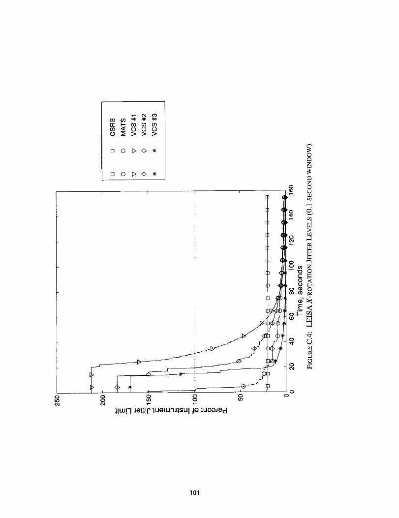
oID
7---
oo04
0 _s 0 > >
[] 0 b 0 •
D 0 bO -_
i f
_J
,_ iro o o
v=. _--
J,!w!7 Je#!r' ;uewnJlsul |o ;ue0Jed
oo
101

ooco
[] 0 b 0 -*-
o 0 b 0 *
i i I I i i
oo
]
]
]
]
]
]
]
)
]
I L
0 O 0 0 0 00 0 0 0 0 0
l!m!l Jeg!r luouJnJ1SUl jo lueoJe d
102

0
O,J
_,_888
I
00
00
103

_888
I I T I I I
00
104

ot(3
T- o4 c)
o_ooo
T
oo
105

ooco
[.) _ > > >
I I I I f I
I0 0 0 00 0 0 0I'_ _ID I_
,,-----'_-- _
I I0 0 00 0 0O0 0,1 .r-
],!w!7 Je_!r :luewnJ:_SUl )o ),USOJS=l
oo
106

oL004
0o >Oo>
o o oo to o
l!tu!q Jell!rluewmlSUl ,to lue0Jed
I
oo
o
107

1- _xI o3
0 0 0
o 0 D 0 -*
o 0 I> 0 *
o(ID
0
Z0
oo00
oo
o o o o o oo o o o o or,_ I.o ._f P) o,1 _.-
1!,,,!-I Jell!r lueuJnJlsUl jo _,ue0Jed
oo
108
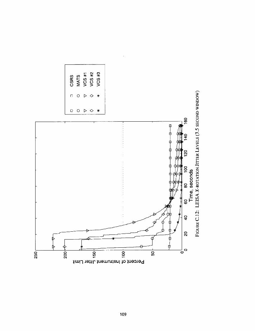
oL0
o o oo uc) o
l!uJ!-I Je}4!r lueLunllsUl 10 lUe0lecl
oL_
00
109

> >
I I ....... I ......
o
o
110

%
0 00 _ >0 > >
[] 0 E> 0 •
[] 0 b 0 •
1
1
7
]
]
]
l
_,!w!7 Je:p,!r' :),ueuJnJ:),SUl _0 ],ueoJe d
f
0
Z0
o o
0
°>
__zo
E<
.1
4/
_ d
o
%,r-
111

112
T--
0 0
n 0 I> 0 •
[] 0 b" 0 •
i ......
S
I ..... , ,
% _o -o
1!W!lJe_1!plueuJnzlsUl_0 lue0Jecl
0
Zo 0
0o
>uJ
o .J
"r--
oJ- L_
d
L_
0
oo
113

_ov--
0 0 0
[] 0 b 0 -_
Q 0 bO -_
I , . . j i i
% %
_!uJ!-IJe_l!p _ueuJnJlsUl _0 _ue0Jed
©
o Z
oT-
u_>
o U_oJ .1
_z8- o
8_-::
o _
o
114

_8880 :_ > > >
[] 0 I>" _ *-
i 1 i '
l!w!7Je_l!r ],ueuJnJ],SUl;0_ue0Jecl
o
o
o
©
Z©
(xl
_Z
>
M
2:0N<
0
<r_
mM
115

_ c0
[] 0 P> _ •
o 0 D 0 •
I
I!Lu!7Je11!PlueuJnJlsUl;olueoJerJ
0r_
o Z
>
H
_i:_ z_
o d
o
116

117

_888
o 0 _> 0 -_
[] 0 b 0 _
0
o Z
u-1
u-1;>
o
.8 z•,- o
00 q} _
E'-
0
ocN
o
118
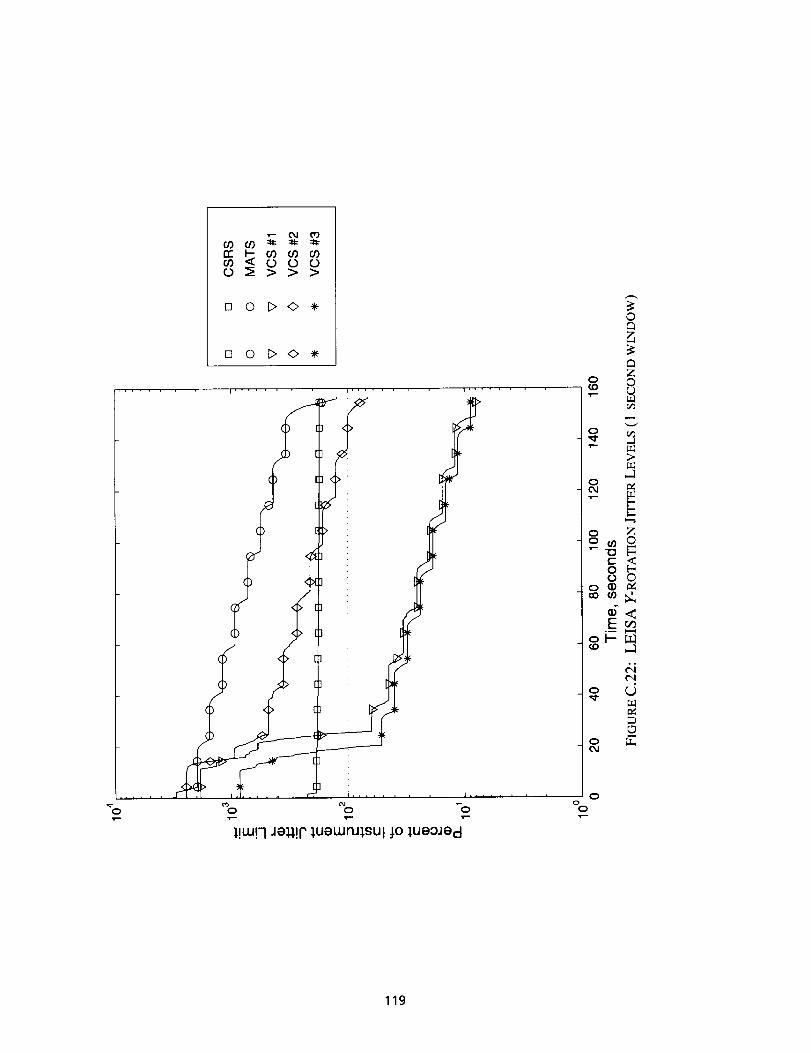
•- oJ 0")
0 o 0
D 0 D'O •
n 0 D'O •
©
Zo ©
uU4
L_
_4
o _C
o_
o_
C4
U_
o
o
ooo
119

0 0 0
oT"
),!uJ!-I Je_l!P lueLunJlSUl jo lueoJed
120

_o
,-- ¢Xl
0 0 0
rq 0 I>_ -_
:l!uJ!7 Je_,!P luewnJJ,SUl ;0 lue0Jecl
0
2
Zo 0
;>
o -1
©
¢xl
_D
ooo
121

I FormApprovedREPORT DOCUMENTATION PAGE O.BNo.0_o_0188
Publicrepor_ngblJrdenforthiscollectionofinformationis estimatedtoaverage1hourperresponse,inc_ucngthe timefor reviewinginstructions,searchingexistingdatasources,gatheringand rnamtainingthe dataneeded,andcompleting andreviewingthe coliec_onofinformation.Se_dcommentsregardingthisburdenestimateor any otheraspectof thiscollectionof information,including suggestionsfor reducingthisburden,to WashingtonHeadquartersServ_:es,Directoratefor InformationOperationsandReports,1215JeffersonDavisHighway,Suite1204, Arlington,VA 22202-4302,and tothe Offk_of ManagementandBudget,Pape"workReductionProject(0704-0188),Washington,De 20503,
1. AGENCY USE ONLY (Leave I_ank) 2. REPORT DATE
Aul_ust 19984. TITLE AND SUBTITLE
Input Shaping to Reduce Solar Array Structural Vibrations
6. AUTHOR(S)
Michael J. Doherty and Robert H. Tolson
7. PERFORMINGORGANIZATIONNAME(S)ANDADDRESS(ES)
The George Washington University
Joint Institute for Advancement of Flight Sciences
NASA Langley Research Center
Hampton, VA 23681-2199
9. SPONSORING/MONITORINGAGENCYNAME(S)ANDADDRESS(ES)
National Aeronautics and Space Administration
Langley Research Center
Hampton, VA 23681-2199
3. REPORT TYPE AND DATES COVERED
Contractor Report5. FUNDING NUMBERS
NCCI-104
632-10-14-28
8. PERFORMING ORGANIZATIONREPORT NUMBER
10. SPONSORINGAIONrrORINGAGENCY REPORT NUMBER
NASA/CR- 1998-208698
11. SUPPLEMENTARY NOTES
The information presented in this report was submitted to the School of Engineering and Applied Science of The
George Washington University in partial fulfillment of the requirements for the Degree of Master of Science,
April 1998. Langley Technical Monitor: Kenny B. Elliott.12a. DISTRIBUTION/AVAILABILITY STATEMENT 12b. DISTRIBUTION CODE
Unclassified-Unlimited
Subject Category 18 Distribution: StandardAvailability: NASA CASI (301) 621-0390
13. ABSTRACT (Maximum 200 words)
Structural vibrations induced by actuators can be minimized using input shaping. Input shaping is a feedforward method
in which actuator commands are convolved with shaping functions to yield a shaped set of commands. These commandsare designed to perform the maneuver while minimizing the residual structural vibration. In this report, input shapingis extended to stepper motor actuators. As a demonstration, an input-shaping technique based on pole-zero cancellationwas used to modify the Solar Array Drive Assembly (SADA) actuator commands for the Lewis satellite. A series ofimpulses were calculated as the ideal SADA output for vibration contr)l. These impulses were then discretized for use bythe SADA stepper motor actuator and simulated actuator outputs were used to calculate the structural response. Theeffectiveness of input shaping is limited by the accuracy of the knowL=dge of the modal frequencies. Assuming perfectknowledge resulted in significant vibration reduction. Errors of 10% in the modal frequencies caused notably higherlevels of vibration. Controller robustness was improved by incorporating additional zeros in the shaping function.The additional zeros did not require increased performance from the actuator. Despite the identification errors, theresulting feedforward controller reduced residual vibrations to the lewl of the exactly modeled input shaper and wellbelow the baseline cases. These results could be easily applied to n_any other vibration-sensitive applicationsinvolving stepper motor actuators.
14. SUBJECT TERMS
Jitter; Control; Input shaping; s/c vibration; Precision pointing
17. SECURITY CLaSSIRCATIOIOF REPORT
Unclassified
NSN 7540-01-280-5500
18. SECURITY CLASSIRCATICNOF TltB PAGE
Unclassified
19. SECURITY CLASSIRCATIONOF ABSTRACT
Uncl_:ssified
15. NUMBER OF PAGES
13616. PRICE CODE
A0720. UMITATION
OF ABSTRACT
Standard Form 298 (Rev. 2-89)PrescribedbyANSI St(l,Z-39-18298-I02
122


![[Array, Array, Array, Array, Array, Array, Array, Array, Array, Array, Array, Array]](https://img.pdfslide.us/doc/110x75/56816460550346895dd63b8b/array-array-array-array-array-array-array-array-array-array-array.jpg)