Embed Size (px)
Citation preview

Input-Output Multipliers, General PurposeTechnologies, and Economic Development
Charles I. Jones*
Department of Economics, U.C. Berkeley and NBERE-mail: [email protected]
http://elsa.berkeley.edu/˜chad
September 24, 2007– Version 0.26
VERY PRELIMINARY AND INCOMPLETE; DO NOT CITE.
Intermediate goods are another produced factor of production, like capital.Simple examples suggest that the multiplier associated with intermediate goodscan be substantial, even larger than the one resulting from physical capital ac-cumulation. This paper evaluates this insight using a model in whichN goodsare produced using all of the other goods as intermediate inputs. Calibratingthe model using detailed input-output tables from the United States and 34 othercountries confirms the importance of the input-output structure of an economyfor economic growth and development. Eleven-fold income differences in a stan-dard neoclassical model become 32-fold differences when intermediate goods aretaken into account.
Key Words:JEL Classification:O40, E10
1. INTRODUCTION
Modern economies involve very sophisticated input-output structures.
Goods like electricity, financial services, transportation, information tech-
nology and healthcare are both inputs and outputs. A wide range of inter-
* I am grateful to John Fernald for helpful conversations about this project and to theToulouse Network for Information Technology and the National ScienceFoundation forfinancial support.
1
2 CHARLES I. JONES
mediate goods are used to produce most goods in the economy, and these
goods in turn are often used as intermediates.
Despite our intuitive recognition of this point, standard models of macroe-
conomics and economic growth typically ignore intermediate goods.1 The
conventional wisdom seems to be that as long as we are concerned about
overall value-added (GDP) in the economy, one can specify the model en-
tirely in terms of value added and ignore intermediate goods. Hence the
neoclassical growth model.
This conventional wisdom is incorrect, and the goal of this paper is to ex-
plore some of the implications of the input-output structure of the economy
for economic growth and development.
The first insight that emerges from thinking about intermediate goods is
that they are very similar to capital. In fact, the only difference between
intermediate goods and capital is one of short-run timing: intermediate
goods can be installed more quickly than capital and “depreciate” fully
during the course of production, while capital takes a bit longer to install
and only partially depreciates during production. From the point of view of
the long run — the perspective relevant in most of this paper — intermediate
goods and capital are essentially the same. In particular, both are produced
factors of production.
The key implications of intermediate goods for economic growth, devel-
opment, and macroeconomics arise from seeing them as another form of
capital. It has long been recognized that the share of capital in production is
a fundamental determinant of the quantitative predictions of macro models.
When the capital share is 1/3, the intrinsic propogation mechanism of the
neoclassical growth model is weak, convergence to the steady state is rapid,
and the model generates a small multiplier on changes in productivity or the
investment rate. In contrast, when the capital share is higher, like 2/3, these
1Exceptions are given at the end of the introduction.
THE INPUT-OUTPUT MULTIPLIER AND ECONOMIC DEVELOPMENT 3
deficiencies are largely remedied. A fairly large portion of the literature
on economic growth can be viewed as an attempt to justify using a (broad)
capital share of 2/3 when the data for (narrow) capital loudly proclaim that
the right number empirically is only 1/3.2
As documented carefully below, the intermediate goods share of gross
output is about 1/2 across a large number of countries. The share of capital
in value-added is about 1/3, so its share in gross output is 1/6. Combining
these two kinds of capital, the share of capital-like goods in gross output
is our magic number,1/2 + 1/6 = 2/3. Incorporating intermediate goods
into macroeconomic models, then, has the potential to help us understand
a range of economic phenomenon, including the propogation of business
cycle shocks and the speed of transition dynamics. These applications will
not be explored here. Instead, the main application in this paper will be to
the great puzzle of understanding why some countries are 50 times richer
than others, as opposed to only 10 times richer.
The paper is organized as follows. The first part provides a simple exam-
ple to illustrate how and why intermediate goods lead to large multipliers.
In this example, a single final output good is used as the single intermediate
good in the economy, so the input-output structure is very simple. The sec-
ond part of the paper builds anN -sector model of economic activity, where
each sector uses the outputs from the other sectors as intermediate goods.
This model is very similar to the original multi-sector business cycle model
of Long and Plosser (1983). The only technological difference is thatwe
include international trade, allowing sectors to import intermediate goods
2For examples of these points in various contexts, see Rebelo (1991), Mankiw, Romerand Weil (1992), Cogley and Nason (1995), and Chari, Kehoe and McGrattan (1997).Mankiw et al. (1992) make many of these points, adding human capital to boost the capitalshare. Chari et al. (1997) introduced “organizational capital” for thesame reason. Howitt(2000) and Klenow and Rodriguez-Clare (2005) consider the accumulation of ideas, anotherproduced factor. More recently, Manuelli and Seshadri (2005) andErosa, Koreshkova andRestuccia (2006) have resurrected the human capital story in a more sophisticated fashion.

4 CHARLES I. JONES
from abroad. The substantive difference is in the application to economic
growth and development.
The third section connects this model to the wealth of input-output data
that exist. Data from 35 countries — including not only the currently
rich countries but also Argentina, Brazil, China, and India — allows us
to quantify the multiplier associated with the input-output structure of the
economy.
The exploration of a last idea is only touched on briefly: connecting the
input-output structure to general purpose technologies. In principle, the
model and data in this paper can answer questions such as, “If there is a one
percentage point improvement in productivity in electric power generation
or in the production of information technology goods, what is the long-run
overall gain in GDP?” To the extent that a good is associated with a “gen-
eral purpose technology” that benefits the economy as a whole, one would
expect these sectoral multipliers to be large. Input-output analysis there-
fore potentially offers one way to quantify the impact of general purpose
technologies. Unfortunately, this analysis has not yet been completed, so
we can only offer some tentative hints at the results that may emerge.3
Before continuing, it is worth noting that there is a very important branch
of the economics literature that has studied the impact of intermediate
goods. Historically, the input-output literature reigned in economics from
the 1930s through the 1960s and is most commonly associated with Leontief
(1936) and his followers. Hirschman (1958) emphasized the importance of
sectoral linkages to economic development, which itself spawned a large
literature. Hulten (1978) is also closely related, in showing how intermedi-
ate goods should properly be included in growth accounting. More recently,
3There is a large literature on general purpose technologies, including David (1990),Bresnahan and Trajtenberg (1995), Jorgenson and Stiroh (1999),Crafts (2004), and manyothers.

THE INPUT-OUTPUT MULTIPLIER AND ECONOMIC DEVELOPMENT 5
the intermediate goods multiplier shows up most clearly in the economic
fluctuations literature; see Long and Plosser (1983), Basu (1995), Horvath
(1998), Dupor (1999), Conley and Dupor (2003), and Gabaix (2005). In the
international trade context, Yi (2003) argues that tariffs can multiply up in
much the same way when goods get traded multiple times during the stages
of production. Ciccone (2002) is closely related to the current paper, deriv-
ing a multiplier formula through intermediate goods for a very particular
input-output structure. Jones (2007) emphasizes the importance of the in-
termediate goods multiplier for a different but very particular input-output
structure.
2. A SIMPLE EXAMPLE
A simple example is quite helpful for understanding how intermediate
goods generate a multiplier. Suppose final outputYt is produced using
capitalKt, laborLt, and intermediate goodsXt.
Yt = A(Kα
t L1−αt
)1−σXσ
t . (1)
Final output can be used for consumption or investment or it can be carried
over to the next period and used as an intermediate good. To keep things
simple, assume a constant fractions of final output is used for investment
and a constant fractionx is used as an intermediate good. Therefore
Kt+1 = sYt + (1 − δ)Kt, (2)
Xt+1 = xYt. (3)
Consumption is then given byCt = (1 − s − x)Yt, and GDP in this
economy is consumption plus investment, or output net of intermediate
goods:(1− x)Yt. In other words, all interesting quantities are proportional
to Yt. Assume labor is exogenous and constant.
6 CHARLES I. JONES
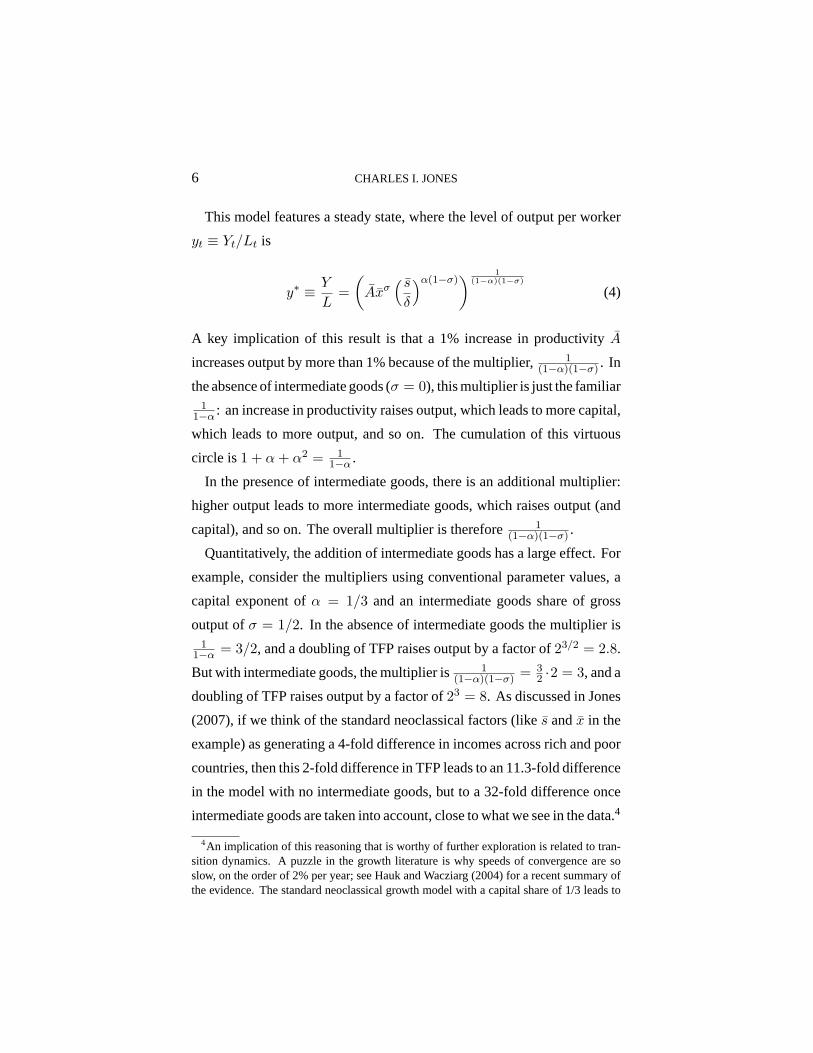
This model features a steady state, where the level of output per worker
yt ≡ Yt/Lt is
y∗ ≡Y
L=
(
Axσ( s
δ
)α(1−σ)) 1
(1−α)(1−σ)
(4)
A key implication of this result is that a 1% increase in productivityA
increases output by more than 1% because of the multiplier,1(1−α)(1−σ) . In
the absence of intermediate goods (σ = 0), this multiplier is just the familiar1
1−α : an increase in productivity raises output, which leads to more capital,
which leads to more output, and so on. The cumulation of this virtuous
circle is1 + α + α2 = 11−α .
In the presence of intermediate goods, there is an additional multiplier:
higher output leads to more intermediate goods, which raises output (and
capital), and so on. The overall multiplier is therefore 1(1−α)(1−σ) .
Quantitatively, the addition of intermediate goods has a large effect. For
example, consider the multipliers using conventional parameter values, a
capital exponent ofα = 1/3 and an intermediate goods share of gross
output ofσ = 1/2. In the absence of intermediate goods the multiplier is1
1−α = 3/2, and a doubling of TFP raises output by a factor of23/2 = 2.8.
But with intermediate goods, the multiplier is 1(1−α)(1−σ) = 3
2 ·2 = 3, and a
doubling of TFP raises output by a factor of23 = 8. As discussed in Jones
(2007), if we think of the standard neoclassical factors (likes andx in the
example) as generating a 4-fold difference in incomes across rich and poor
countries, then this 2-fold difference in TFP leads to an 11.3-fold difference
in the model with no intermediate goods, but to a 32-fold difference once
intermediate goods are taken into account, close to what we see in the data.4
4An implication of this reasoning that is worthy of further exploration is relatedto tran-sition dynamics. A puzzle in the growth literature is why speeds of convergence are soslow, on the order of 2% per year; see Hauk and Wacziarg (2004) fora recent summary ofthe evidence. The standard neoclassical growth model with a capital share of 1/3 leads to

THE INPUT-OUTPUT MULTIPLIER AND ECONOMIC DEVELOPMENT 7
The deeper question in this paper is whether this multiplier carries over
into a model with a rich and realistic input-output structure. Perhaps the
input-output structure in practice does not lead to these large feedback
effects. Or perhaps importing intermediate goods dilutes the multiplier
substantially in practice. In fact, the remainder of this paper shows that
these concerns are not important in practice. The simple “one over one
minus the intermediate goods share” formula suggested by this example
turns out to be a very good approximation to the true input-output multiplier
in modern economies.
3. THE FULL INPUT-OUTPUT MODEL
Assume the economy consists ofN sectors. Each sector uses capital,
labor, domestic intermediate goods, and imported intermediate goods to
produce output. In turn, this output can be used for final consumption or
as an intermediate good in production.
Given this general picture, we specialize to a particular structure with
two goals in mind: analytic tractability and obtaining a model that can be
closely connected to the rich input-output data. To these ends, the model
augments the original Long and Plosser (1983) business cycle model, based
on Cobb-Douglas production functions, by embedding it in a model with
trade.
We begin by describing the economic environment and then allocate
resources using a competitive equilibrium with taxes.
a speed of convergence of about 7% per year. The presence of intermediate goods wouldslow this rate down, just as it raises the multiplier. (A difficulty in quantifying thiseffectis the question of how long it takes to produce and use intermediate goods: one week, onemonth, or one year? That is, how long is a period?)

8 CHARLES I. JONES
3.1. The Economic Environment
Each of theN sectors produces with the following Cobb-Douglas tech-
nology:
Yi = Ai
(
Kαi
i H1−αi
i
)1−σi−λi
dσi1i1 dσi2
i2 · ... · dσiN
iN︸ ︷︷ ︸
domestic IG
mλi1i1 mλi2
i2 · ... · mλiN
iN︸ ︷︷ ︸
imported IG(5)
wherei indexes the sector.Ai is an exogenous productivity term, which
itself is the product of aggregate productivityA and sectoral productivityηi:
Ai ≡ Aηi. Ki andHi are the quantities of physical and human capital used
in sectori. Two kinds of intermediate goods are used in production:dij is
the quantity of domestic goodj used by sectori, andmij is the quantity of
the imported intermediate goodj used by sectori. (We assume imported
intermediate goods are different, so that they are not perfect substitutes;
this fits with the empirical fact that countries both import and produce
intermediate goods in narrow 6-digit categories.) We abuse notation by
assuming there areN different intermediate goods that can be imported
and by indexing these byj as well. The parameter values in this production
function satisfyσi ≡∑N
j=1 σij andλi ≡∑N
j=1 λij and0 < αi < 1, so
the production function features constant returns to scale.
Each domestically produced good can be used for final consumption,cj ,
or can be used as an intermediate good:
cj +N∑
i=1
dij = Yj , j = 1, . . . , N. (6)
Rather than specifying a utility function over theN different consumption
goods and performing a formal national income accoutning exercise, it is
more convenient to aggregate these final consumption goods into a single
final good through another log-linear production function:
Y = cβ11 · ... · cβN
N , (7)

THE INPUT-OUTPUT MULTIPLIER AND ECONOMIC DEVELOPMENT 9
where∑N
i=1 βi = 1.
This aggregate final good can itself be used in one of two ways, as con-
sumption or exported to the rest of the world:
C + X = Y. (8)
It is these exports that pay for the imported intermediate goods. We think
of this (static) model as describing the long-run steady state of a model, so
we impose balanced trade:
PX =N∑
i=1
N∑
j=1
pjmij , (9)
whereP is the exogenous world price of the final good andpj is the ex-
ogenous world price of the imported intermediate goods.
Finally, we assume fixed, exogenous supplies of physical and human
capital (for now):N∑
i=1
Ki = K, (10)
N∑
i=1
Hi = H. (11)
3.2. A Competitive Equilibrium with Taxes
To allocate resources in this economy, we will focus on a competi-
tive equilibrium with tax distortions. As in Chari, Kehoe and McGrattan
(forthcoming), Hsieh and Klenow (2006), Lagos (2006), and Restuccia and
Rogerson (2007), tax distortions at the micro (here sectoral) level can aggre-
gate up to provide differences in TFP. Sector-specific taxes could literally
be taxes, but they could also represent any kind of policy that favors one
sector over another (regulations, special consideration for credit, and so
on). The additional insight here is that these differences can be multiplied
by the input-output structure of the economy.
10 CHARLES I. JONES
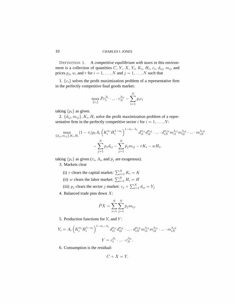
Definition 1. A competitive equilibrium with taxesin this environ-ment is a collection of quantitiesC, Y , X, Yi, Ki, Hi, ci, dij , mij andpricespj , w, andr for i = 1, . . . , N andj = 1, . . . , N such that
1. {ci} solves the profit maximization problem of a representative firmin the perfectly competitive final goods market:
max{ci}
P cβ11 · ... · cβN
N −N∑
i=1
pici
taking{pi} as given.2. {dij , mij}, Ki, Hi solve the profit maximization problem of a repre-
sentative firm in the perfectly competitive sectori for i = 1, . . . , N :
max{dij ,mij},Ki,Hi
(1 − τi)piAi
(
Kαi
i H1−αi
i
)1−σi−λi
dσi1i1 dσi2
i2 · ... · dσiN
iN mλi1i1 mλi2
i2 · ... · mλiN
iN
−N∑
j=1
pjdij −N∑
j=1
pjmij − rKi − wHi,
taking{pi} as given (τi, Ai, andpj are exogenous).3. Markets clear
(i) r clears the capital market:∑N
i=1 Ki = K
(ii) w clears the labor market:∑N
i=1 Hi = H
(iii) pj clears the sectorj market:cj +∑N
i=1 dij = Yj
4. Balanced trade pins downX:
PX =
N∑
i=1
N∑
j=1
pjmij .
5. Production functions forYi andY :
Yi = Ai
(
Kαi
i H1−αi
i
)1−σi−λi
dσi1i1 dσi2
i2 · ... · dσiN
iN mλi1i1 mλi2
i2 · ... · mλiN
iN
Y = cβ11 · ... · cβN
N .
6. Consumption is the residual:
C + X = Y.

THE INPUT-OUTPUT MULTIPLIER AND ECONOMIC DEVELOPMENT 11
Counting loosely, there are 12 equilibrium objects to be determined and
12 equations implicit in this equilibrium definition. Hiding behind the last
equation is the fact that tax revenues are rebated lump sum to households.
Because of balanced trade, however, there is no decision for households
to make regarding final consumptionC, and it is simply determined as the
residual of final output less exports.5
3.3. Solving
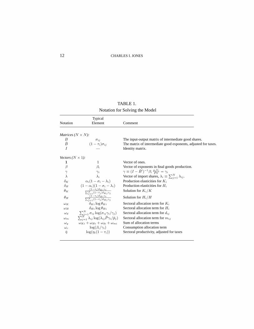
In solving for the equilibrium of the model, it is useful to define some
notation involving linear algebra. This is summarized in Table 1. Then the
following proposition characterizes the equilibrium:
Proposition 1 (Solution forY andC). In the competitive equilib-
rium, the solution for total production of the aggregate final good is
Y = AµKαH1−αǫ, (12)
where the following notation applies:
µ′ ≡ β′(I−B)−1
1−β′(I−B)−1λ, (N × 1 vector of multipliers)
µ ≡ µ′1
α ≡ µ′δK
ω ≡β′ωc+β′(I−B)−1ωy
1−β′(I−B)−1λ
log ǫ ≡ ω + µ′η.
Moreover, GDP for this economy is given byC, which equals
C = Y
1 −N∑
i=1
N∑
j=1
(1 − τi)γiλij
. (13)
5I presume this equation could be replaced byPC = wH + rK + T , whereT is thelump sum rebate. zzz Check.
12 CHARLES I. JONES
TABLE 1.
Notation for Solving the Model
TypicalNotation Element Comment
Matrices (N × N ):B σij The input-output matrix of intermediate good shares.B (1 − τi)σij The matrix of intermediate good exponents, adjusted for taxes.I — Identity matrix.
Vectors (N × 1):1 1 Vector of ones.β βi Vector of exponents in final goods production.γ γi γ ≡ (I − B′)−1β; piYi
PY= γi
λ λi Vector of import shares,λi ≡PN
j=1 λij .δK αi(1 − σi − λi) Production elasticities forKi
δH (1 − αi)(1 − σi − λi) Production elasticities forHi
θK(1−τi)δKiγi
P
Nj=1
(1−τj)δKjγjSolution forKi/K
θH(1−τi)δHiγi
P
Nj=1
(1−τj)δHjγjSolution forHi/H
ωK δKi log θKi Sectoral allocation term forKi
ωH δHi log θHi Sectoral allocation term forHi
ωd
PN
j=1 σij log(σijγi/γj) Sectoral allocation term fordij
ωm
PN
j=1 λij log(λijP γi/pj) Sectoral allocation term formij
ωy ωKi + ωHi + ωdi + ωmi Sum of allocation termsωc log(βi/γi) Consumption allocation termη log(ηi(1 − τi)) Sectoral productivity, adjusted for taxes
THE INPUT-OUTPUT MULTIPLIER AND ECONOMIC DEVELOPMENT 13
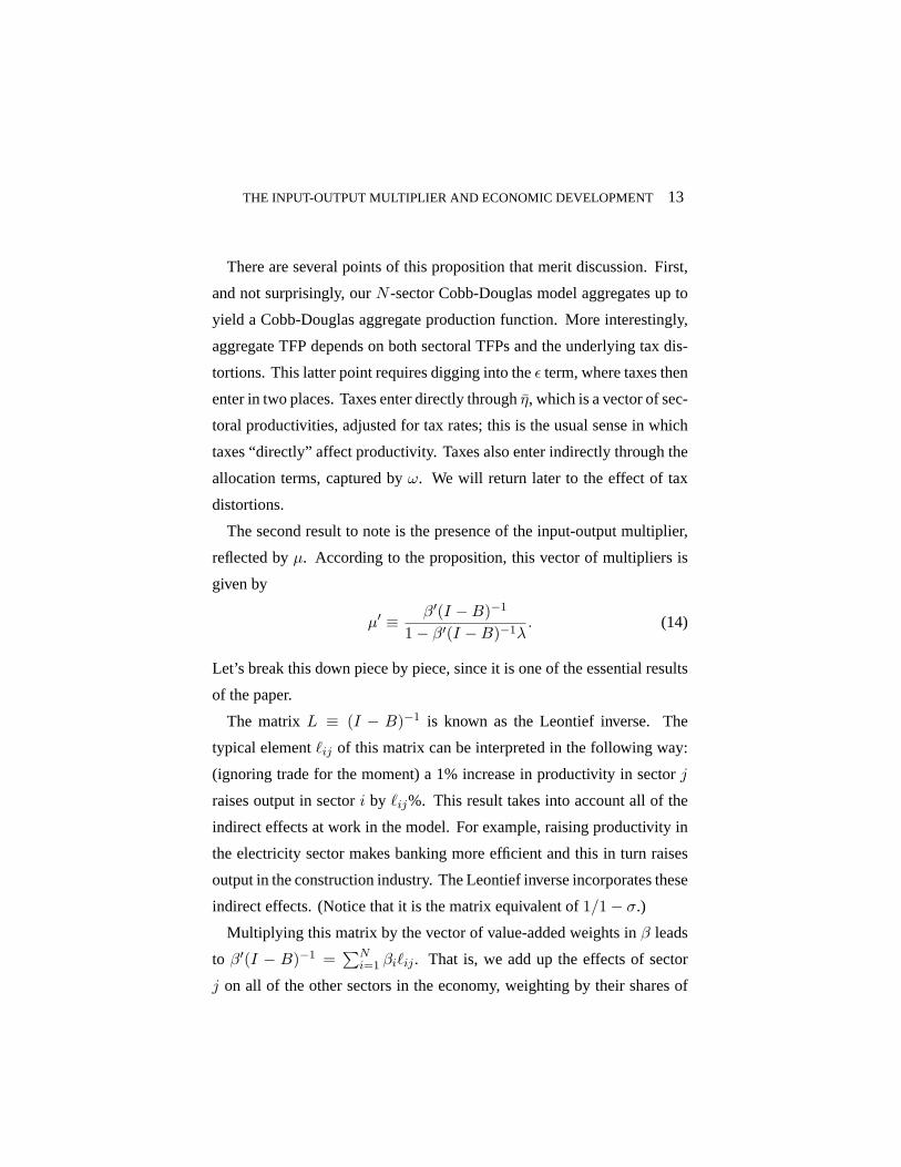
There are several points of this proposition that merit discussion. First,
and not surprisingly, ourN -sector Cobb-Douglas model aggregates up to
yield a Cobb-Douglas aggregate production function. More interestingly,
aggregate TFP depends on both sectoral TFPs and the underlying tax dis-
tortions. This latter point requires digging into theǫ term, where taxes then
enter in two places. Taxes enter directly throughη, which is a vector of sec-
toral productivities, adjusted for tax rates; this is the usual sense in which
taxes “directly” affect productivity. Taxes also enter indirectly throughthe
allocation terms, captured byω. We will return later to the effect of tax
distortions.
The second result to note is the presence of the input-output multiplier,
reflected byµ. According to the proposition, this vector of multipliers is
given by
µ′ ≡β′(I − B)−1
1 − β′(I − B)−1λ. (14)
Let’s break this down piece by piece, since it is one of the essential results
of the paper.
The matrixL ≡ (I − B)−1 is known as the Leontief inverse. The
typical elementℓij of this matrix can be interpreted in the following way:
(ignoring trade for the moment) a 1% increase in productivity in sectorj
raises output in sectori by ℓij%. This result takes into account all of the
indirect effects at work in the model. For example, raising productivity in
the electricity sector makes banking more efficient and this in turn raises
output in the construction industry. The Leontief inverse incorporates these
indirect effects. (Notice that it is the matrix equivalent of1/1 − σ.)
Multiplying this matrix by the vector of value-added weights inβ leads
to β′(I − B)−1 =∑N
i=1 βiℓij . That is, we add up the effects of sector
j on all of the other sectors in the economy, weighting by their shares of
14 CHARLES I. JONES
value-added. The typical element of this multiplier matrix then reveals
how a change in producitivity in sectorj affects overall value-added in the
economy.
All of this would be precisely correct ifλij were zero — that is, in the
absence of trade. In the presense of trade, this multiplier gets adjusted by
the factor1/(1−β′(I −B)−1λ). We will discuss this factor in more detail
below, but for now it is enough to note that this factor is larger than one:
trade strengthens the multiplier rather than attenuating it.
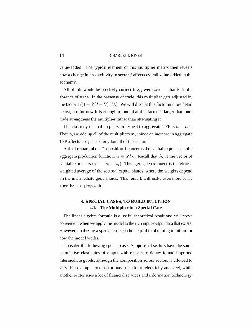
The elasticity of final output with respect to aggregate TFP isµ ≡ µ′1.
That is, we add up all of the multipliers inµ since an increase in aggregate
TFP affects not just sectorj but all of the sectors.
A final remark about Proposition 1 concerns the capital exponent in the
aggregate production function,α ≡ µ′δK . Recall thatδK is the vector of
capital exponentsαi(1 − σi − λi). The aggregate exponent is therefore a
weighted average of the sectoral capital shares, where the weights depend
on the intermediate good shares. This remark will make even more sense
after the next proposition.
4. SPECIAL CASES, TO BUILD INTUITION4.1. The Multiplier in a Special Case
The linear algebra formula is a useful theoretical result and will prove
convenient when we apply the model to the rich input-output data that exists.
However, analyzing a special case can be helpful in obtaining intuition for
how the model works.
Consider the following special case. Suppose all sectors have the same
cumulative elasticities of output with respect to domestic and imported
intermediate goods, although the composition across sectors is allowed to
vary. For example, one sector may use a lot of electricity and steel, while
another sector uses a lot of financial services and information technology.
THE INPUT-OUTPUT MULTIPLIER AND ECONOMIC DEVELOPMENT 15
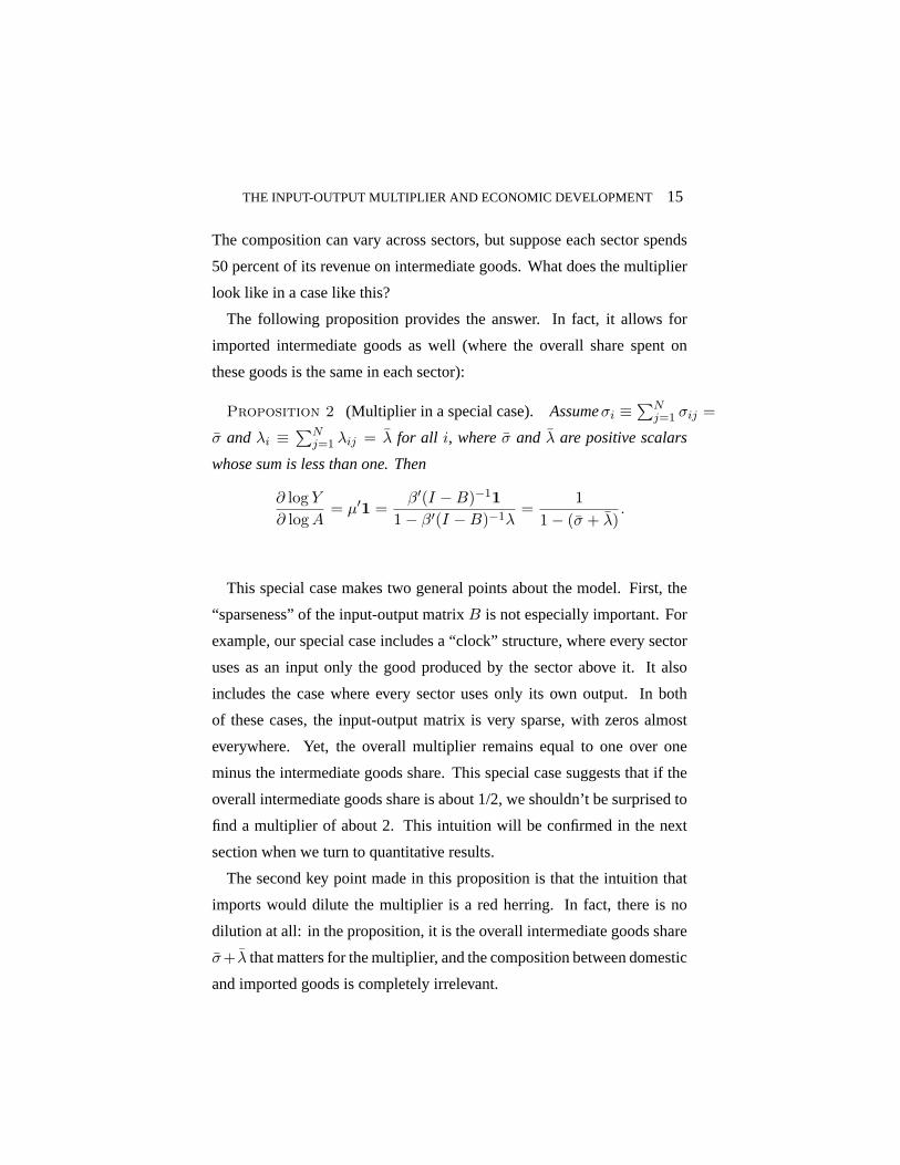
The composition can vary across sectors, but suppose each sector spends
50 percent of its revenue on intermediate goods. What does the multiplier
look like in a case like this?
The following proposition provides the answer. In fact, it allows for
imported intermediate goods as well (where the overall share spent on
these goods is the same in each sector):
Proposition 2 (Multiplier in a special case). Assumeσi ≡∑N
j=1 σij =
σ andλi ≡∑N
j=1 λij = λ for all i, whereσ and λ are positive scalars
whose sum is less than one. Then
∂ log Y
∂ log A= µ′
1 =β′(I − B)−1
1
1 − β′(I − B)−1λ=
1
1 − (σ + λ).
This special case makes two general points about the model. First, the
“sparseness” of the input-output matrixB is not especially important. For
example, our special case includes a “clock” structure, where every sector
uses as an input only the good produced by the sector above it. It also
includes the case where every sector uses only its own output. In both
of these cases, the input-output matrix is very sparse, with zeros almost
everywhere. Yet, the overall multiplier remains equal to one over one
minus the intermediate goods share. This special case suggests that if the
overall intermediate goods share is about 1/2, we shouldn’t be surprised to
find a multiplier of about 2. This intuition will be confirmed in the next
section when we turn to quantitative results.
The second key point made in this proposition is that the intuition that
imports would dilute the multiplier is a red herring. In fact, there is no
dilution at all: in the proposition, it is the overall intermediate goods share
σ+ λ that matters for the multiplier, and the composition between domestic
and imported goods is completely irrelevant.
16 CHARLES I. JONES
Why is this the case? The answer is that we have imposed balanced trade
in our (long run) model. Therefore exports are used to “produce” imports.
A higher productivity in the domestic computer chip sector raises overall
exports, which in turn increases imports, so the virtuous circle is not broken
by the presence of trade.6
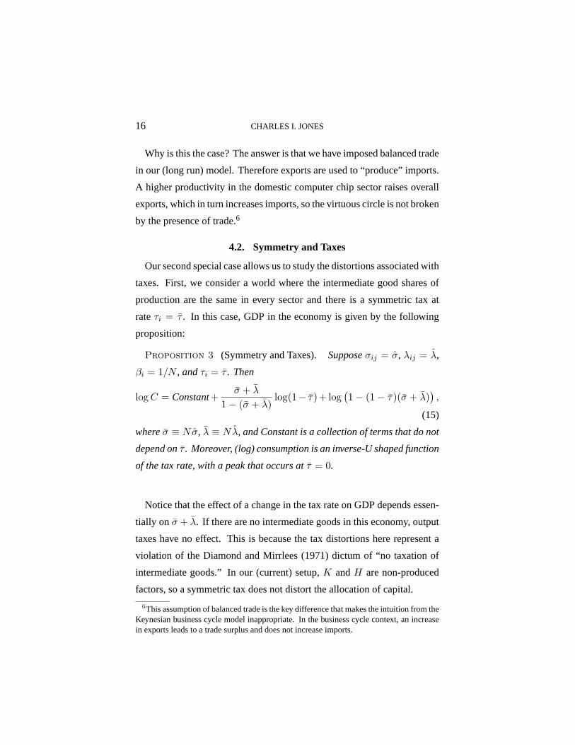
4.2. Symmetry and Taxes
Our second special case allows us to study the distortions associated with
taxes. First, we consider a world where the intermediate good shares of
production are the same in every sector and there is a symmetric tax at
rateτi = τ . In this case, GDP in the economy is given by the following
proposition:
Proposition 3 (Symmetry and Taxes). Supposeσij = σ, λij = λ,
βi = 1/N , andτi = τ . Then
log C = Constant+σ + λ
1 − (σ + λ)log(1− τ)+ log
(1 − (1 − τ)(σ + λ)
),
(15)
whereσ ≡ Nσ, λ ≡ Nλ, and Constant is a collection of terms that do not
depend onτ . Moreover, (log) consumption is an inverse-U shaped function
of the tax rate, with a peak that occurs atτ = 0.
Notice that the effect of a change in the tax rate on GDP depends essen-
tially on σ + λ. If there are no intermediate goods in this economy, output
taxes have no effect. This is because the tax distortions here representa
violation of the Diamond and Mirrlees (1971) dictum of “no taxation of
intermediate goods.” In our (current) setup,K andH are non-produced
factors, so a symmetric tax does not distort the allocation of capital.
6This assumption of balanced trade is the key difference that makes the intuition from theKeynesian business cycle model inappropriate. In the business cycle context, an increasein exports leads to a trade surplus and does not increase imports.

THE INPUT-OUTPUT MULTIPLIER AND ECONOMIC DEVELOPMENT 17
The key distortion is between consumption and intermediate goods. A
good that gets consumed pays the tax only once when the good is produced;
a good that is used as an intermediate pays the tax when it is first produced
then when it is used as an intermediate. Since a constant fraction of output is
consumed and the rest is used as an intermediate good, this process suffers
from the vicious cycle of the multiplier.
(Note for a future version: Physical capital is certainly a produced factor,
and it is very much like an intermediate good. Hence the right “number”
to plug in for σ + λ is probably 2/3: the intermediate goods share plus
the capital share. Taking into account the portion of human capital that
is produced using output, the share would be even larger; labor could be
distorted as well if there were a labor-leisure decision.)
Symmetric taxes affect GDP through the two terms in equation (15). The
first term is the direct effect, where taxes enter the model very much like
productivity: recall that both1 − τi andAi are subject to the multiplier
effect through theǫ term in Proposition 1. The second term mitigates this
effect somewhat and captures the indirect effect whereby higher taxes raise
consumption (by reducing the purchase of intermediate goods).
4.3. Symmetry with Random Taxes
Our final special case allows us to consider variation in taxes across
sectors. Suppose everything in the model other than taxes is symmetric,
and allow taxes to be a log-normally distributed random variable:
Proposition 4 (Symmetry with Random Taxes).Supposeσij = σ,
λij = λ, andβi = 1/N . Assumelog(1 − τi) ∼ N(θ, v2). Then
plimN→∞ log C = C ≡Constant+σ + λ
1 − (σ + λ)· θ
+ log(
1 − (σ + λ)eθ+ 12v2
)
−1
2v2,
18 CHARLES I. JONES
whereσ ≡ Nσ, λ ≡ Nλ, and Constant is a collection of terms that do not
depend onθ or v2. Moreover, consumption is maximized when there are
no taxes; also∂C∂v2 < 0.
In terms of the mean effect of taxes, this result looks very much like the
previous one. Now, however, we have an additional result related to thevari-
ance of taxes across sectors. In particular, a higher variance of taxes reduces
GDP, even in the absence of intermediate goods, since random taxes will
distort the allocation of capital and labor across sectors. However, the vari-
ance term itself is subject to a multiplier effect:∂C∂v2 = −1
2 ·(
11−(σ+λ)(1−τ)
)
,
whereτ is the average tax rate. A higher variance of taxes is more costly
in an economy with intermediate goods. This makes sense: the first best
in this economy is to have no taxes. Either a constant tax or a random
tax distorts the allocation of resources and reduces GDP. The magnitude
of the distortion depends on the Diamond-Mirrlees effect: how important
intermediate goods are in production.
5. QUANTITATIVE ANALYSIS
We now turn to the rich input-output data that exists, both for the United
States and for many other countries. This data allows us to calculate aggre-
gate and sectoral multipliers and to study the effect of sectoral tax distortions
on aggregate GDP. First, we use the six-digit level data available from the
U.S. Bureau of Economic Analysis for the United States in 1997. Then
we turn to the OECD Input-Output Database, which contains data for 48
industries and 35 countries.
THE INPUT-OUTPUT MULTIPLIER AND ECONOMIC DEVELOPMENT 19
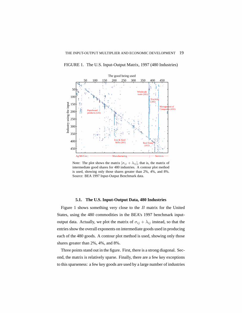
FIGURE 1. The U.S. Input-Output Matrix, 1997 (480 Industries)
The good being used
Indu
stry
usi
ng th
e in
put
Wholesale trade (381)
Trucking(385)
Management ofCompanies (431)
Real Estate (411)
Iron & Steel Mills (201)
Paperboardproducts (125)
Ag/Mi/Con | −−−−−−−−−−−−−−−− Manufacturing −−−−−−−−−−−−−−− | −−− Services −−−
50 100 150 200 250 300 350 400 450
50
100
150
200
250
300
350
400
450
Note: The plot shows the matrix[σij + λij ], that is, the matrix ofintermediate good shares for 480 industries. A contour plot methodis used, showing only those shares greater than 2%, 4%, and 8%.Source: BEA 1997 Input-Output Benchmark data.
5.1. The U.S. Input-Output Data, 480 Industries
Figure 1 shows something very close to theB matrix for the United
States, using the 480 commodities in the BEA’s 1997 benchmark input-
output data. Actually, we plot the matrix ofσij + λij instead, so that the
entries show the overall exponents on intermediate goods used in producing
each of the 480 goods. A contour plot method is used, showing only those
shares greater than 2%, 4%, and 8%.
Three points stand out in the figure. First, there is a strong diagonal. Sec-
ond, the matrix is relatively sparse. Finally, there are a few key exceptions
to this sparseness: a few key goods are used by a large number of industries
20 CHARLES I. JONES
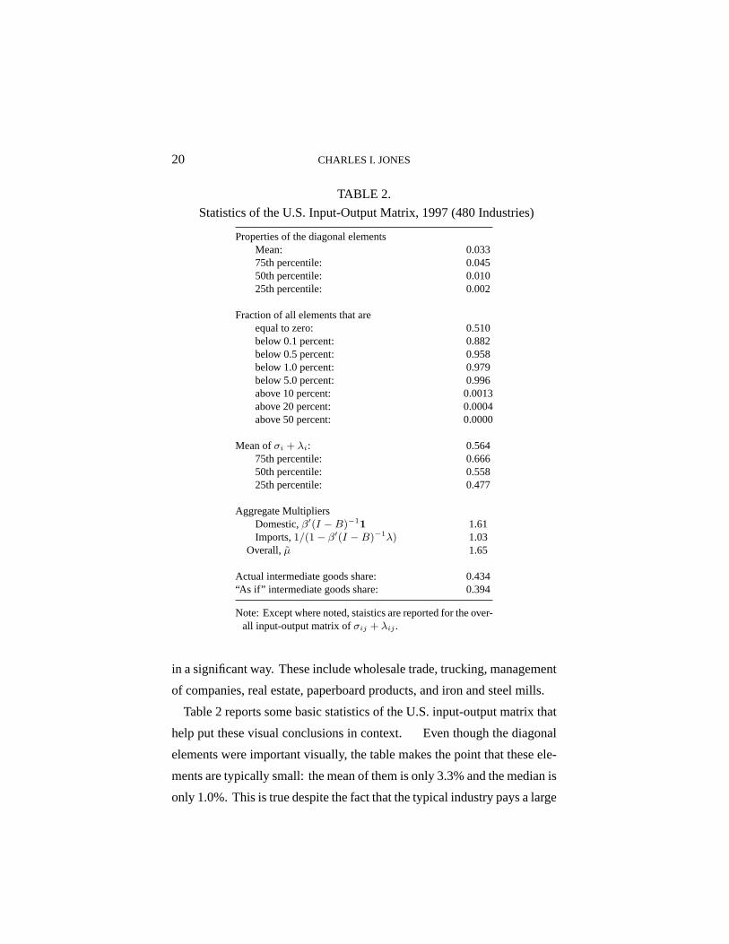
TABLE 2.
Statistics of the U.S. Input-Output Matrix, 1997 (480 Industries)
Properties of the diagonal elementsMean: 0.03375th percentile: 0.04550th percentile: 0.01025th percentile: 0.002
Fraction of all elements that areequal to zero: 0.510below 0.1 percent: 0.882below 0.5 percent: 0.958below 1.0 percent: 0.979below 5.0 percent: 0.996above 10 percent: 0.0013above 20 percent: 0.0004above 50 percent: 0.0000
Mean ofσi + λi: 0.56475th percentile: 0.66650th percentile: 0.55825th percentile: 0.477
Aggregate MultipliersDomestic,β′(I − B)−1
1 1.61Imports,1/(1 − β′(I − B)−1λ) 1.03
Overall,µ 1.65
Actual intermediate goods share: 0.434“As if” intermediate goods share: 0.394
Note: Except where noted, staistics are reported for the over-all input-output matrix ofσij + λij .
in a significant way. These include wholesale trade, trucking, management
of companies, real estate, paperboard products, and iron and steel mills.
Table 2 reports some basic statistics of the U.S. input-output matrix that
help put these visual conclusions in context. Even though the diagonal
elements were important visually, the table makes the point that these ele-
ments are typically small: the mean of them is only 3.3% and the median is
only 1.0%. This is true despite the fact that the typical industry pays a large
THE INPUT-OUTPUT MULTIPLIER AND ECONOMIC DEVELOPMENT 21
share of its gross output to intermediate goods: 56.4% at the mean. The
industry at the 75th percentile pays out about two-thirds of its revenue to in-
termediate goods, while even the industry at the 25th percentile pays nearly
half. Along these lines, it is worth noting that even though just 0.13% of
the elements of the input-output matrix exceed 10 percent, this is still 288
elements over all; similarly, 83 of the entries are greater than 20 percent.
As the bottom of the table shows, the overall intermediate goods share for
the U.S. economy is about 43.4%: service industries are more important as
a share of value-added, and these industries have lower intermediate goods
shares.
The last part of the table computes the aggregate multiplier using the
6-digit input-output data. A 1% improvement in TFP in every sector raises
overall GDP by 1.65%. This number is the product of a domestic multiplier
of 1.61 (that would obtain if no intermediate goods were imported), and
an import multiplier of 1.03. Imports are relatively unimportant in the
multiplier.
To what extent is the simple 11−(σ+λ)
formula accurate? The multiplier of
1.65 would result from this formula “if” the intermediate goods share were
0.394. In fact, the intermediate goods share using this 6-digit data is 0.434.
This simple aggregate formula appears to give a good approximation to the
result found by computing the 480x480 Leontief inverse, although there is
a small degree of dilution: applying the formula to the 0.434 share suggests
a multiplier that overstates the truth by about ten percent.
5.2. General Purpose Technologies?
To what extent can the input-output structure of the economy help us
to understand general purpose technologies? The answer is unclear.To
the extent that the adoption of a general purpose technology leads to other
changes in the structure of production, this may not be directly apparent

22 CHARLES I. JONES
in the input-output structure. For example, a common hypothesis is that
the adoption of electricity or information technology leads to fundamental
changes in the nature and/or organization of production. Perhaps such
changes will not be apparent.
On the other hand, perhaps they will. Sectoral multipliers — theµi
terms in the model — should represent something like a first-order or local
derivative of output with respect to a particular productivity level. If the
production function really is Cobb-Douglas, then this local derivative could
extend more broadly. Or if we had input-output tables from 1970 or 1900,
perhaps tracing the path of the local derivatives would be informative. (In
fact, the BEA does provide benchmark input-output tables every five years,
going back to 1967 at least. So it should be possible to explore the GPT
nature of information technologies in more detail.)
Table 3 provides some detail on the sectoral multipliers,µi. In partic-
ular, we find the sectors that have the largest excess multiplier — that is,
the sectors whereµi − βi is the largest. (Recall that a 1% increase in pro-
ductivity in sectori raises output byβ% directly because of this sector’s
role in final consumption. So the net multiplier effect from the input-output
structure of the economy subtracts this off.) Important sectors according
to this measure include real estate, wholesale trade, management of com-
panies, and advertising. Just below that are telecommunications, oil and
gas extraction, power generation, banking, trucking, and legal services. All
seem like sectors that are generally important in the production of a wide
range of goods in the economy. In this sense, the sectoral multipliers may
indeed be telling us something about general purpose technologies.
For comparison, we also report the multipliers for some industries related
to information technology at the bottom of the table. These multipliers are
small for two reasons. First, the share of these industries in value-added
is small, so the direct effect is already small. Second, and perhaps more

THE INPUT-OUTPUT MULTIPLIER AND ECONOMIC DEVELOPMENT 23
TABLE 3.
U.S. Input-Output Multipliers, 1997 (480 Industries)
Excess V.A. — IntGood Shares —Multiplier Multiplier Share Domestic Import
Industry µi − βi µi βi σi λi
Real estate 0.043 0.094 0.051 0.306 0.003Wholesale trade 0.034 0.091 0.057 0.356 0.009Management of companies 0.029 0.056 0.027 0.291 0.004Advertising services 0.020 0.032 0.011 0.446 0.012Telecommunications 0.018 0.036 0.018 0.394 0.013Oil and gas extraction 0.014 0.018 0.004 0.579 0.016Power generation/supply 0.013 0.030 0.017 0.355 0.010Banking (depository) 0.013 0.042 0.029 0.271 0.003Truck transportation 0.012 0.022 0.010 0.501 0.011Legal services 0.011 0.024 0.013 0.276 0.003
Information Technology IndustriesComputer manufacturing ... 0.001 0.001 0.845 0.016Computer storage devices ... 0.001 0.001 0.619 0.054Other computer equipment ... 0.001 0.001 0.662 0.074Semiconductors ... 0.011 0.006 0.351 0.030Software publishers ... 0.005 0.005 0.305 0.022Custom programming ... 0.008 0.008 0.294 0.024

24 CHARLES I. JONES
importantly, many of the products of information technology (including
software) are capital goods, not intermediate goods . To compute the true
multipliers associated with these sectors, one would need to know how
much capital each sector produces and where that capital is used. These
calculations are possible, using the capital flow table provided by the BEA.
However, I haven’t yet had a chance to do these calculations.7
5.3. The OECD Input-Output Data, 48 Industries
The 2006 edition of the OECD Input-Output Database contains input-
output data for 35 countries and 48 industries, typically for the year 2000.
In addition to covering OECD countries, the data also include some poor
and middle-income countries, such as China, India, Argentina, Brazil, and
Russia.
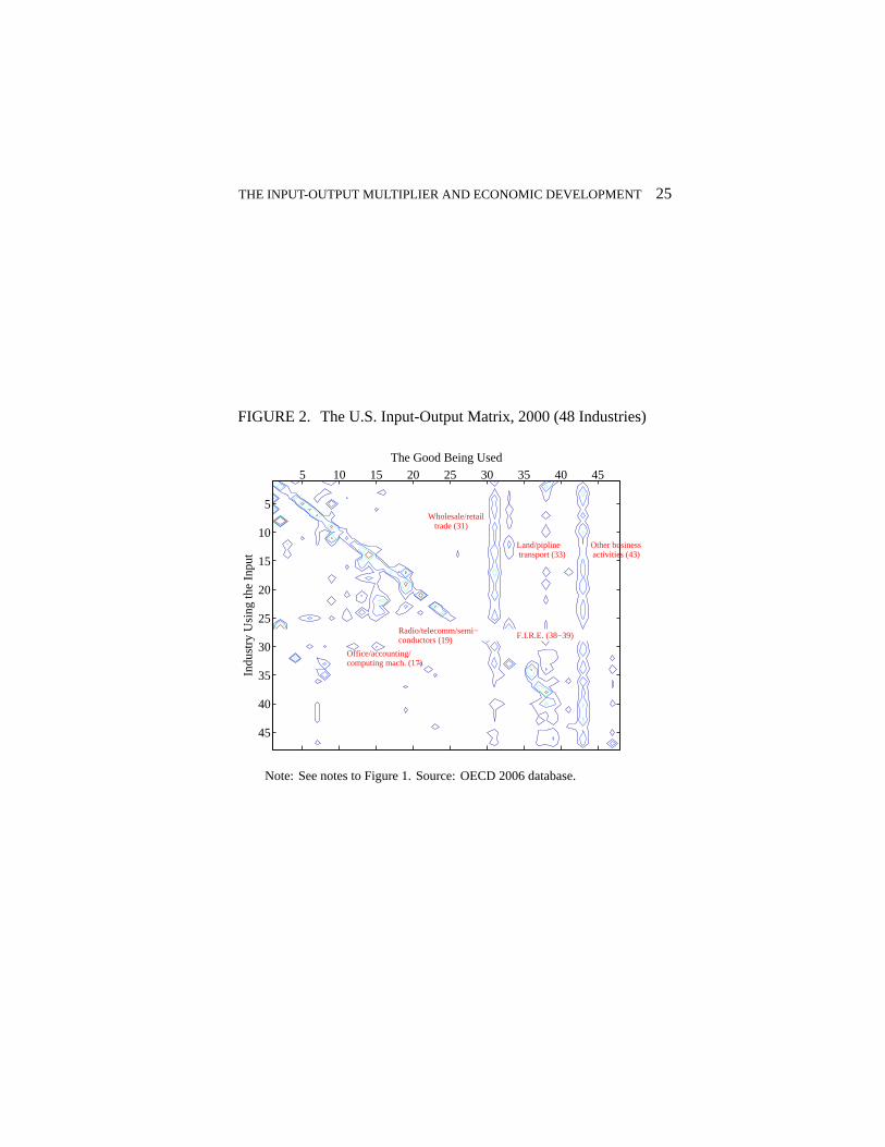
Figure 2 shows the input-output matrix for the United States at this higher
level of aggregation. The pattern at the more detailed level of aggregation
of a sparse matrix with a strong diagonal and just a few goods that are used
widely is repeated at this higher level of aggregation.
One of the nice features of the OECD data is that we can consider the ques-
tion of how much the input-output structure of an economy differs across
countries. The general and perhaps surprising answer that one obtains is
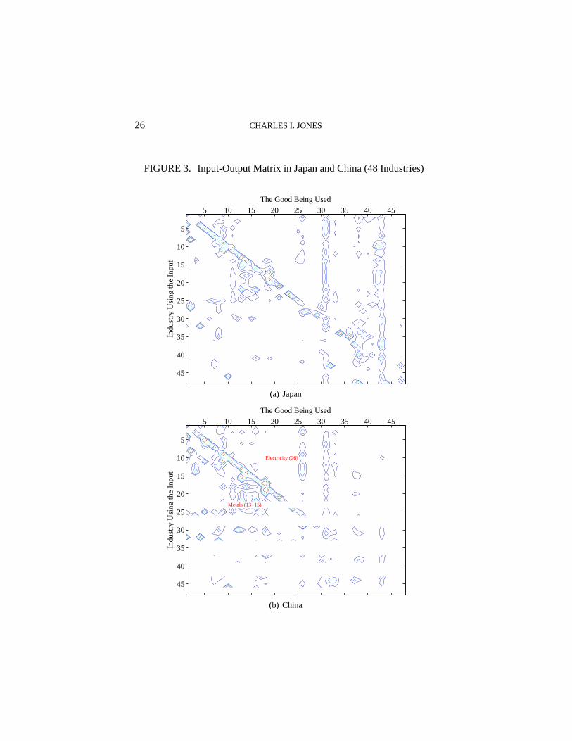
“not much.” Figure 3 shows the input-output matrix for two countries,
Japan and China, as an example.
The matrix for Japan looks very much like the matrix for the United
States. This is true more generally, especially for the richer countries in
the data set. But it is even true for the poorer countries. The input-output
7U.S. BEA has a “capital flow” matrix which essentially decomposes private investmentinto a CxI use table. (Some aggregation issues). If we really want to pursue the GPT andindustry multiplier logic, then incorporating the capital flow matrix is an obviousnext step.(Question: rK/Y versus pI/Y — if we just treat capital as an intermediate good, we will gettoo low a share.)
THE INPUT-OUTPUT MULTIPLIER AND ECONOMIC DEVELOPMENT 25
FIGURE 2. The U.S. Input-Output Matrix, 2000 (48 Industries)
Indu
stry
Usi
ng th
e In
put
The Good Being Used
Wholesale/retail trade (31)
Other business activities (43)
Land/pipline transport (33)
Office/accounting/computing mach. (17)
Radio/telecomm/semi−conductors (19) F.I.R.E. (38−39)
5 10 15 20 25 30 35 40 45
5
10
15
20
25
30
35
40
45
Note: See notes to Figure 1. Source: OECD 2006 database.
26 CHARLES I. JONES
FIGURE 3. Input-Output Matrix in Japan and China (48 Industries)In
dust
ry U
sing
the
Inpu
t
The Good Being Used5 10 15 20 25 30 35 40 45
5
10
15
20
25
30
35
40
45
(a) Japan
Indu
stry
Usi
ng th
e In
put
The Good Being Used
Electricity (26)
Metals (13−15)
5 10 15 20 25 30 35 40 45
5
10
15
20
25
30
35
40
45
(b) China

THE INPUT-OUTPUT MULTIPLIER AND ECONOMIC DEVELOPMENT 27
matrix for China is perhaps the most different from the United States, but
the overall structure is still similar. Electricity shows up as being noticeably
more important, and other business activities (which include advertising,
accounting, and legal services) as somewhat less important. These are the
main differences.
The first column of Table 4 makes these comparisons more systematically.
It shows the fraction of elements in the input-output matrix that differ by
more than 0.02 from the corresponding elements in the U.S. input-output
matrix. Just over 16 percent of the elements exceed this difference in
China’s input-output matrix, while the corresponding number for Japan is
about 9 percent. For this level of the cutoff, the average across the 35
countries is 11 percent. If we lower the cutoff to 0.01, the typical country
has differences of this magnitude in just over 20 percent of the cells. If we
raise the cutoff to 0.05, the average across countries is 3.9 percent of cells.
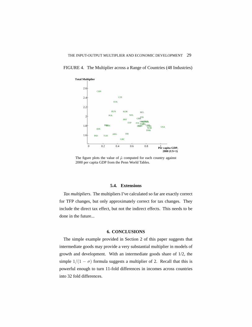
Figure 4 shows the aggregate multipliers,µ for the 35 countries in our
sample. The average value for the multiplier in this sample is about 1.9.
It ranges from a high of 2.53 in China to lows of 1.51 in Greece and 1.59
in India. Interestingly, China and India are two of the poorest countries in
the sample, and they have widely different multipliers. The multiplier for
the United States using this data works out to be 1.77, slightly higher than
what we found in the 6-digit data.
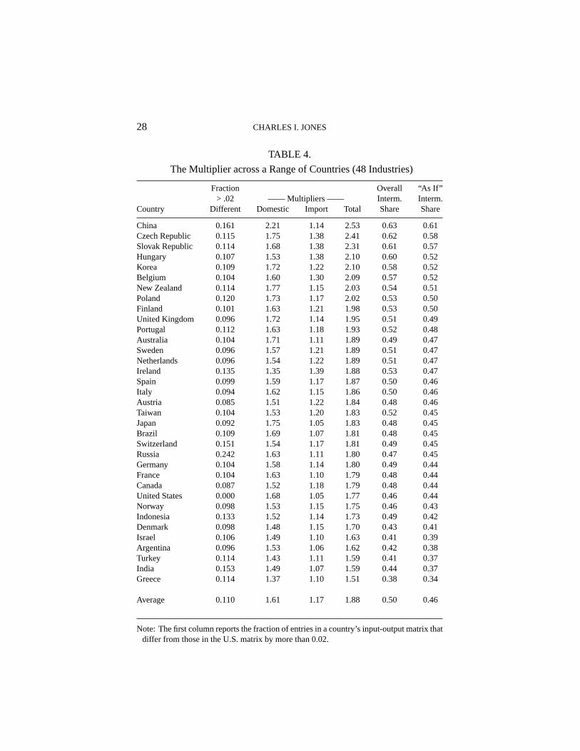
Table 4 shows these multipliers in more detail, including the contribution
from imported intermediate goods as well as the aggregate intermediate
goods share and the “as if” share that corresponds to the multiplier computed
using the Leontief inverse. The simple approximation of “one over one
minus the intermediate goods share” does a very good job of approximating
the true multiplier.
zzz The general similarity of these matrices across countries suggests
that C-D not too bad...
28 CHARLES I. JONES
TABLE 4.
The Multiplier across a Range of Countries (48 Industries)
Fraction Overall “As If”> .02 —— Multipliers —— Interm. Interm.
Country Different Domestic Import Total Share Share
China 0.161 2.21 1.14 2.53 0.63 0.61Czech Republic 0.115 1.75 1.38 2.41 0.62 0.58Slovak Republic 0.114 1.68 1.38 2.31 0.61 0.57Hungary 0.107 1.53 1.38 2.10 0.60 0.52Korea 0.109 1.72 1.22 2.10 0.58 0.52Belgium 0.104 1.60 1.30 2.09 0.57 0.52New Zealand 0.114 1.77 1.15 2.03 0.54 0.51Poland 0.120 1.73 1.17 2.02 0.53 0.50Finland 0.101 1.63 1.21 1.98 0.53 0.50United Kingdom 0.096 1.72 1.14 1.95 0.51 0.49Portugal 0.112 1.63 1.18 1.93 0.52 0.48Australia 0.104 1.71 1.11 1.89 0.49 0.47Sweden 0.096 1.57 1.21 1.89 0.51 0.47Netherlands 0.096 1.54 1.22 1.89 0.51 0.47Ireland 0.135 1.35 1.39 1.88 0.53 0.47Spain 0.099 1.59 1.17 1.87 0.50 0.46Italy 0.094 1.62 1.15 1.86 0.50 0.46Austria 0.085 1.51 1.22 1.84 0.48 0.46Taiwan 0.104 1.53 1.20 1.83 0.52 0.45Japan 0.092 1.75 1.05 1.83 0.48 0.45Brazil 0.109 1.69 1.07 1.81 0.48 0.45Switzerland 0.151 1.54 1.17 1.81 0.49 0.45Russia 0.242 1.63 1.11 1.80 0.47 0.45Germany 0.104 1.58 1.14 1.80 0.49 0.44France 0.104 1.63 1.10 1.79 0.48 0.44Canada 0.087 1.52 1.18 1.79 0.48 0.44United States 0.000 1.68 1.05 1.77 0.46 0.44Norway 0.098 1.53 1.15 1.75 0.46 0.43Indonesia 0.133 1.52 1.14 1.73 0.49 0.42Denmark 0.098 1.48 1.15 1.70 0.43 0.41Israel 0.106 1.49 1.10 1.63 0.41 0.39Argentina 0.096 1.53 1.06 1.62 0.42 0.38Turkey 0.114 1.43 1.11 1.59 0.41 0.37India 0.153 1.49 1.07 1.59 0.44 0.37Greece 0.114 1.37 1.10 1.51 0.38 0.34
Average 0.110 1.61 1.17 1.88 0.50 0.46
Note: The first column reports the fraction of entries in a country’s input-output matrix thatdiffer from those in the U.S. matrix by more than 0.02.
THE INPUT-OUTPUT MULTIPLIER AND ECONOMIC DEVELOPMENT 29
FIGURE 4. The Multiplier across a Range of Countries (48 Industries)
0 0.2 0.4 0.6 0.8 1
1.6
1.8
2
2.2
2.4
2.6
ARG
AUSAUT
BEL
BRA CANCHE
CHN
CZE
GER
DNK
ESP
FIN
FRA
GBR
GRC
HUN
IDN
IND
IRL
ISR
ITAJPN
KOR
NLD
NOR
NZLPOL
PRT
RUS
SVK
SWE
TUR
USA
Per capita GDP,2000 (US=1)
Total Multiplier
The figure plots the value ofµ computed for each country against2000 per capita GDP from the Penn World Tables.
5.4. Extensions
Tax multipliers. The multipliers I’ve calculated so far are exactly correct
for TFP changes, but only approximately correct for tax changes. They
include the direct tax effect, but not the indirect effects. This needs to be
done in the future...
6. CONCLUSIONS
The simple example provided in Section 2 of this paper suggests that
intermediate goods may provide a very substantial multiplier in models of
growth and development. With an intermediate goods share of 1/2, the
simple1/(1 − σ) formula suggests a multiplier of 2. Recall that this is
powerful enough to turn 11-fold differences in incomes across countries
into 32 fold differences.
30 CHARLES I. JONES
The question considered in the main part of the paper is whether this sim-
ple formula holds up when one considers the detailed input-output structure
of modern economies. The answer is that it does: the average multiplier
in the 35 countries for which we have data, for example, is 1.88, ranging
from a low of about 1.6 in India to a high of about 2.5 in China. The input-
output multiplier, then, may be an important part of a theory of economic
development.
There are numerous directions for additional research suggested by this
analysis. Sectoral multipliers and the multipliers on idiosynchratic tax
distortions have barely been explored. Do some sectors, like electricity
or information technology, have a particularly significant role that can be
detected in the input-output tables? Would distortions to the allocation of
resources in these sectors have large negative effects on GDP? How different
are the input-output structures across economies? Why do China and India
have such different structures, while the rich countries, especially, seem
much more similar? How have these input-output structures changed over
time?
APPENDIX: PROOFS
Proposition 1: Solving forY andC.
Proof. To be provided.
Proposition 2: The Multiplier in a Special Case.
Proof. In matrix notation, the assumption that all sectors have a cumu-
lative domestic intermediate goods share ofσ is simplyB1 = σ1. This
THE INPUT-OUTPUT MULTIPLIER AND ECONOMIC DEVELOPMENT 31
implies the following:
(I − B)1 = (1 − σ)1
1 = (I − B)−11 · (1 − σ)
1 = β′1 = β′(I − B)−1
1 · (1 − σ)
⇒ β′(I − B)−11 =
1
1 − σ.
Similarly, β′(I − B)−1λ = λ1−σ . Therefore
µ′1 =
β′(I − B)−11
1 − β′(I − B)−1λ=
1
1 − (σ + λ).
Proposition 3: Symmetric and Taxes.
Proof. The key step in solving the model is to use the same general result
as in the previous proposition: if a matrixX has rows that sum to the same
value,x, then(I−X)−11 = 1 · 1
1−x . In this case, this result is used in com-
putingγ = (I − B)−1β, whereβi = 1/N . Everything else follows from
careful calculation.
REFERENCES
Basu, Susanto, “Intermediate Goods and Business Cycles: Implications for Produc-tivity and Welfare,”American Economic Review, June 1995,85 (3), 512–531.
Bresnahan, Timothy F. and M. Trajtenberg, “General purposetechnologies ’En-gines of growth’?,”Journal of Econometrics, January 1995,65 (1), 83–108.
Chari, V.V., Pat Kehoe, and Ellen McGrattan, “The Poverty ofNations: A Quan-titative Investigation,” 1997. Working Paper, Federal Reserve Bank of Min-neapolis.
, , and , “Business Cycle Accounting,”Econometrica, forthcoming.
Ciccone, Antonio, “Input Chains and Industrialization,”Review of Economic Stud-ies, July 2002,69 (3), 565–587.
32 CHARLES I. JONES
Cogley, Timothy and James M Nason, “Output Dynamics in Real-Business-CycleModels,”American Economic Review, June 1995,85 (3), 492–511.
Conley, Timothy G. and Bill Dupor, “A Spatial Analysis of Sectoral Complemen-tarity,” Journal of Political Economy, April 2003,111(2), 311–352.
Crafts, Nicholas, “Steam as a general purpose technology: Agrowth accountingperspective,”Economic Journal, 2004,114(495), 338–351.
David, Paul A., “The Dynamo and the Computer: An Historical Perspective on theModern Productivity Paradox,”American Economic Association Papers andProceedings, May 1990,80 (2), 355–361.
Diamond, Peter A. and James A. Mirrlees, “Optimal Taxation and Public ProductionI: Production Efficiency,”American Economic Review, March 1971,61(1), 8–27.
Dupor, Bill, “Aggregation and irrelevance in multi-sectormodels,”Journal of Mon-etary Economics, April 1999,43 (2), 391–409.
Erosa, Andres, Tatyana Koreshkova, and Diego Restuccia, “On the Aggregateand Distributional Implications of Productivity Differences Across Countries,”2006. University of Toronto working paper.
Gabaix, Xavier, “The Granular Origins of Aggregate Fluctuations,” 2005. MITworking paper.
Hauk, William R. and Romain Wacziarg, “A Monte Carlo Study ofGrowth Re-gressions,” January 2004. NBER Technical Working Paper No.296.
Hirschman, Albert O.,The Strategy of Economic Development, New Haven, CT:Yale University Press, 1958.
Horvath, Michael T.K., “Cyclicality and Sectoral Linkages: Aggregate Fluctuationsfrom Independent Sectoral Shocks,”Review of Economic Dynamics, October1998,1 (4), 781–808.
Howitt, Peter, “Endogenous Growth and Cross-Country Income Differences,”American Economic Review, September 2000,90 (4), 829–846.
Hsieh, Chang-Tai and Peter J. Klenow, “Misallocation and Manufacturing TFP inChina and India,” June 2006. University of California at Berkeley workingpaper.
Hulten, Charles R., “Growth Accounting with Intermediate Inputs,” Review ofEconomic Studies, 1978,45 (3), 511–518.
Jones, Charles I., “The Weak Link Theory of Economic Development,” 2007. U.C.Berkeley working paper.
THE INPUT-OUTPUT MULTIPLIER AND ECONOMIC DEVELOPMENT 33
Jorgenson, Dale W. and Kevin J. Stiroh, “Information Technology and Growth,”American Economic Association Papers and Proceedings, May 1999,89 (2),109–115.
Klenow, Peter J. and Andres Rodriguez-Clare, “Extenalities and Growth,” inPhilippe Aghion and Steven Durlauf, eds.,Handbook of Economic Growth,Amsterdam: Elsevier, 2005.
Lagos, Ricardo, “A Model of TFP,”Review of Economic Studies, 2006,73 (4),983–1007.
Leontief, Wassily, “Quantitative Input and Output Relations in the Economic Sys-tem of the United States,”Review of Economics and Statistics, 1936,18 (3),105–125.
Long, John B. and Charles I. Plosser, “Real Business Cycles,” Journal of PoliticalEconomy, February 1983,91 (1), 39–69.
Mankiw, N. Gregory, David Romer, and David Weil, “A Contribution to the Em-pirics of Economic Growth,”Quarterly Journal of Economics, May 1992,107(2), 407–438.
Manuelli, Rodolfo and Ananth Seshadri, “Human Capital and the Wealth of Na-tions,” March 2005. University of Wisconsin working paper.
Rebelo, Sergio, “Long-Run Policy Analysis and Long-Run Growth,” Journal ofPolitical Economy, June 1991,99, 500–521.
Restuccia, Diego and Richard Rogerson, “Policy Distortions and Aggregate Pro-ductivity with Heterogeneous Plants,” April 2007. NBER Working Paper13018.
Yi, Kei-Mu, “Can Vertical Specialization Explain the Growth of World Trade?,”Journal of Political Economy, February 2003,111(1), 52–102.