Embed Size (px)
Citation preview

Input Diffusion and the Evolution of
Production Networks∗
Vasco M. Carvalho Nico VoigtländerCambridge and CEPR UCLA, NBER, and CEPR
First Version: March 2014This Version: February 2015
Abstract
The adoption and diffusion of inputs in the production network is at the heart of technological
progress. What determines which inputs are initially considered and eventually adopted by inno-
vators? We examine the evolution of input linkages from a network perspective, starting from a
stylized model of network formation. Producers direct their search for new inputs along vertical
linkages, screening the network neighborhood of existing suppliers to identify potentially useful
inputs. A subset of these is then adopted, following a tradeoff between the benefits from input
variety and the costs of customizing new inputs. Guided by this framework, we document a novel
stylized fact at both the sector and the firm level: producersare more likely to adopt inputs that are
already used – directly or indirectly – by their current suppliers. In particular, using disaggregated
input-output data, we show that initial network proximity of a sector in 1967 significantly increases
the likelihood of adoption throughout the subsequent four decades. A one-standard deviation de-
crease in network distance is associated with an increase inthe adoption probability by one third to
one half. Similarly, U.S. firms are significantly more likelyto develop new input linkages among
their suppliers’ network neighborhood. Our results imply that the existing production network
plays a crucial role in the diffusion of inputs and the evolution of technology.
JEL: O33, C67, D57, L23
Keywords: Input adoption, directed network search, dynamics of production networks
∗We would like to thank Daron Acemoglu, Ufuk Akcigit, Enghin Atalay, Sanjeev Goyal, Ali Hortaçsu, Ali Jad-babaie, Chad Jones, Ezra Oberfield, Michael Peters, GiacomoPonzetto, Alireza Tahbaz-Salehi and Jaume Ventura, aswell as seminar participants at CREI, the NBER Summer Institute, the NBER EFJK Growth Group, the SED meetingin Seoul, and the University of Cambridge for helpful comments and suggestions. Carvalho acknowledges the finan-cial support of the European Research Council grant #337054, the Cambridge-INET Institute, and the Keynes Fellow-ship at the University of Cambridge. Voigtländer acknowledges support from the UCLA Anderson Easton TechnologyLeadership Program. We are grateful to Ali Hortaçsu and Enghin Atalay for sharing their data on supplier-to-customerlinkages.

1 Introduction
The adoption of new inputs is an important dimension of technological progress. This is true for
both product innovation – where the integration of new inputs leads to new or improved output –
and for process innovation, where new inputs can raise the efficiency of production. Input-output
linkages are also important for macroeconomic outcomes: they can amplify idiosyncratic sectoral
distortions into large aggregate productivity differences (Ciccone, 2002; Jones, 2011, 2013), and
they can create aggregate fluctuations by propagating micro-level shocks (Acemoglu, Carvalho,
Ozdaglar, and Tahbaz-Salehi, 2012). Yet, input linkages are typically taken as given; little is
known about the evolution of production networks.1
In this paper, we analyze the formation of input linkages. Weask what determines which inputs
are initially considered and eventually adopted in the production of new or improved goods.2 Sim-
ilarly, why are some inputs so much more prominent than others?3 We take a network perspective
to answer these questions. To structure our analysis, we build on a standard network formation
argument and hypothesize that producers direct their search for new inputs to the network neigh-
bourhood of their existent suppliers. Guided by this stylized model, we explore the empirical
determinants of new input link formation both at the sector and the firm level. We uncover a strik-
ing empirical regularity: producers are more likely to adopt inputs that are already used upstream
– directly or indirectly – by their current suppliers. By thesame token, we find that inputs that are
initially closer to many potential adopters are more likelyto diffuse widely. Our results imply that
the existing input-output network plays a key role in the formation of new linkages.
To guide our analysis, we provide a stylized model of networkformation at the variety level
and then explore its sector-level implications. Each variety producer is embedded in a network of
production linkages – producers do not only interact directly with their suppliers, but also indirectly
with input producers further upstream. This gives rise to the notion of network distance between
any potentialbuyer-supplier pair, i.e., a producer’s distance to inputsthat are not (yet) directly
used. In order to keep the analysis simple, we take the arrival of new varieties as given and focus
on their input adoption decisions. In each period, a new variety emerges exogenously. It then
1The exceptions areAtalay, Hortaçsu, Roberts, and Syverson(2011) and Oberfield(2013); both examine theevolution of linkages at the firm level. For a recent overviewof the literature on production networks seeCarvalho(2014).
2Firms often experiment with several potentially suitable inputs before making their final choice. For example,Steve Jobs famously had the first iPhone’s screen changed from plastic to hardened glass only four weeks before massproduction began in 2007.
3The number of sectors that source inputs from a given supplier follows a power law (Carvalho, 2010). Atalayet al.(2011) andKelly, Lustig, and Van Nieuwerburgh(2013) report evidence on the distribution of supply linkages atthe firm level. The power law in the outdegree distribution iscrucial for linkages to augment idiosyncratic shocks intoaggregate fluctuations (Acemoglu et al., 2012).
1

forms input linkages following three steps, where the first two build on the central mechanism of
a class of dynamic network formation models. We illustrate these steps in the graph below. First,
a new variety producer (j) draws a set of ‘essential’ input suppliers (nodesg andh). Second,
in order to customize its new variety,j searches for further potentially useful inputs among the
suppliers ofg andh (i.e., among nodesa-e). In other words, the search is directed vertically in
the production network, towards the technological neighborhood of essential inputs. Third, the
new variety producerj decides which inputs to adopt among those identified in the second step.
This decision is driven by a trade-off between the benefits from a larger set of input varieties (à la
Romer, 1990) and variety-specific customization costs for each adoptedinput. As a result, a finite
optimal number of inputs is adopted (indicated by the dashedarrows).
"networkneighborhood"
a b c d e
j’s essential inputs g h
new producer j
input flows� �
eventuallyadopted�
This process implies that individual producers are more likely to adopt inputs that are closer
in their network neighborhood. This is similar to the evolution of social networks, where new
friendships are more likely to form with friends of friends than with random people. In the context
of production, a firm is more likely to adopt an input that its supplier is already using, than a random
input from the product universe. The formation of new linkages delivers a law of motion, where
the current production network and its evolution are closely interrelated: on the one hand, present
network distances determine input adoption; input adoption, on the other hand, changes network
distances. This gives rise to a dynamic evolution of the input-output network. The stylized model
also delivers a power law in the number of varieties supplied, in line with the empirical regularities
observed byCarvalho, Nirei, Saito, and Tahbaz-Salehi(2014).
We then explore the sector-level implications of the variety-level mechanism. To define sectors
in the model, we build on the rules by which new commodities are assigned to sectors in actual
input-output tables. This classification is based on a variety’s essential inputs. For example, a
new variety that draws tires, an engine, and a body will be assigned to the motor vehicles sector.
We show that, based on this definition, the model predicts i) new input linkages across sectors are
more likely to emerge within the proximity of existent inputsupply relations and ii) the power
2

law distribution of forward linkages aggregates up to the sector-level. Thus, even if the underlying
network formation is happening at thevarietylevel, we can make use ofsectoralinput-output data
to examine the model’s predictions.
Following the theoretical framework, our empirical analysis examines the determinants of in-
put adoption at the sector and firm level. We first use U.S. input-output tables at the 4-digit level
between 1967 and 2002. Based on the observed intersectoral linkages in manufacturing, we com-
pute a standard measure of network distance between any sector pair. We find that sectors are
substantially more likely to adopt inputs that are initially closer in their input-output network. This
is illustrated in Figure1. On the x-axis we plot the simplest possible measure of network distance
in 1967 – the smallest number of directed input links separating a (potential) input supplieri from
a (potential) input adopterj. This provides a simple metric for the vertical distance between an
upstream supplier and a downstream potential user of the input. For example, in 1967, the sec-
tor "Primary Batteries, Dry and Wet" (SIC 3692) had distance2 to the (potential adopter) sector
"X-Ray Apparatus" (SIC 3844), while it had distance 4 to "Cigarettes" (SIC 2111). The y-axis
gives the frequency of input adoption events (j adoptingi) observed after 1967.4 For example,
in our data we observe that "X-Ray Apparatus" producers adopted "Primary Batteries, Dry and
Wet" as an input in 1977, while "Cigarettes" never did so. Thepattern in Figure1 is striking.
Input adoption is much more frequent for sector-pairs that were already relatively close (but not
yet directly trading inputs) in the 1967 input-output network. For 22% of sector-pairs that were
two input-links apart in 1967 (distance 2),j adoptedi over the subsequent 35 year period.5 This is
more than double the frequency of adoption observed for distance-3-sectors (9%), and more than
5 times the frequency observed for sectors that were 5 links apart.
Our main finding holds both in a panel setting where the input-output network evolves over
time, and also in a cross-sectional analysis showing that closer network proximity in 1967 re-
duces the subsequent time to adoption. Our results are robust to alternative definitions of network
distance and adoption. They are also unaffected by a host of controls such as size, proxies for tech-
nological progress, as well as fixed effects for adopting andinput-producing sectors. Throughout,
we document economically significant magnitudes; for example, a one-standard deviation decrease
in network distance raises the adoption probability in any given 5-year period by one third to one
half.
4We say that a sectorj adopts inputi if there was no input flow fromi to j in 1967, and such a flow is recorded atany point thereafter in our sample, which extends until 2002.
5Not all of these ‘adoptions’ are long-lived; many reflect one-time input flows between sectors. All our findingsare robust to alternative definition of adoption. In particular, our most conservative definition requires input flows ofatleast $1million over at least 15 years. In this case, the frequency of adoption for distance 2 is 4.9%, and – consistentlywith the differential pattern in Figure1 – it is significantly lower for larger distances.
3

Next, we examine the formation of supplier linkages at thefirm level. We use data from Com-
pustat, which includes information on major customers – those that are responsible for more than
10% of a given seller’s revenues. Because of this reporting threshold, the analysis is naturally lim-
ited to relatively important links. Based on this data, we construct a network of suppliers and their
customers. We confirm that firms are significantly more likelyto adopt inputs that have previously
been used by their suppliers (close network proximity) thaninputs from outside their network
neighborhood. Additionally, we show that our findings are robust to the inclusion of firm-level
controls, such as fixed effects, firm size, labor productivity, or the geographical distance between
firm pairs.
Our analysis shares a common limitation with other studies of production networks: exogenous
variation for input-output linkages is not available. Thisraises the concern of omitted variable
bias. For example, a general trend towards computerizationmay be accompanied by a gradual
spread of electronic components as inputs in production. Since these are in turn connected to
semiconductors, this process would bring sectors closer tothe latter in the input-output network,
with some of them eventually directly adopting semiconductors. While this would confound our
panel results, it is less likely to affect our results that are based exclusively on initial network
distance in 1967. In fact, technological trends would only affect these results if they were related
to initial network distance. But this, in turn, is the core ofour argument – initial network distance
matters for the future evolution of linkages. In addition, we show that our results also hold when
we include sector-pair fixed effects, so that we exploit onlychangesin network distance, i.e., the
variation that is due to new links forming or existing links disappearing over time. Consequently,
unobserved correlates ofinitial network distance are also unlikely to explain the pattern inthe
data. These findings impose restriction on interpretationsof our results: candidates to explain the
empirical regularities have to be correlated with network distance (both in levels and changes), and
be related to direct adoption of inputs. We discuss three interpretations that fit this pattern.
First, network distance may reflect technological distancein the sense that production processes
are more or less similar, rendering ‘closer’ inputs more compatible. For example, the production
of valves is technologically closer to vehicles than food processing, making the former a more
feasible input in car production. Second, network distancecould proxy for spatial distance to
the extent that industries and firms that trade inputs intensively tend to coagglomerate (Ellison,
Glaeser, and Kerr, 2010). Third, network proximity may reflect more frequent socialinteractions
through which information about potentially useful inputsis transmitted. A second limitation of
our analysis is that, ultimately, we cannot distinguish between these mechanisms. Nevertheless,
we can narrow down possible interpretations. The fact that geographical distance between firms
does not change our results makes coagglomeration unlikelyas a main driver. At the sector level,
4

we show that excluding linkages formed within the same 2-digit sector does not affect our findings;
we also show that the forward-distance between sectors (i.e., links via buyers, instead of suppliers)
does not predict input adoption. This implies that horizontal similarity of sectors is not a likely
candidate to explain the pattern in the data. Rather, our results suggest thatverticaldistance along
supply chains is a useful starting point to understand patterns of input adoption and diffusion.
We build on a rich research agenda that has studied the diffusion of technology, starting from
the seminal work byGriliches(1957). A macro strand of this literature has focused on how par-
ticular technologies – such as electricity or semi-conductors – are progressively adopted by an
expanding range of sectors. This gives rise to General Purpose Technologies (GPT) that mark
historical eras and are seen as engines of growth (Helpman and Trajtenberg, 1998; Jovanovic and
Rousseau, 2005). As in this literature, we are interested in understandinghow a particular technol-
ogy can emerge as an input supplier to many other technologies.6 Our results imply that occupying
a relatively central position in the production network – for example, when a new input is used
by already central technologies – makes wide diffusion morelikely. Our paper is also related to
a micro strand of the literature that focuses on the role of social networks in the adoption of par-
ticular technologies (c.f.Young, 2003; Conley and Udry, 2010; Banerjee, Chandrasekhar, Duflo,
and Jackson, 2013). We share the view that the adoption of technologies is mediated through
a network. However, rather than focusing on the role of localsocial interactions, we study the
importance of distance in the technological network more broadly.7
We also naturally relate to a literature that models the evolution of technology as a recombi-
natoric process of existing ideas into new ones (Weitzman, 1998).8 The large number of possible
combinations ledWeitzmanto the conclusion that "the ultimate limits to growth may lienot so
much in our abilities to generate new ideas, as in our abilities to process to fruition an ever in-
creasing abundance of potentially fruitful ideas" [p.359]. This begs the question of how innovators
organize their ‘search process’ among the myriad of possible combinations. Our approach makes
6Interestingly, whileHelpman and Trajtenberg(1998) rationalize the staggered diffusion of a GPT in terms ofasymmetric adoption costs, they also conjecture that the order of adoption could be the result of "linkages betweenadopting sectors" and thus, that "technological proximity" may be an important factor in explaining diffusion patternsof GPTs. Our key mechanism formalizes this notion of "technological proximity" by placing technologies in a networkand emphasizing network proximity as a key driver of adoption.
7As discussed above, proximity in the input-output network may also reflect more frequent social interaction. Forexample, a tire producer is more likely to interact with people from the automotive industry than with pharmaceuticalstaff. Our argument exploits the variation acrosssector pairs, whereas the micro literature on social networks examinesthe role of local social interactions for the adoption of agiventechnology. SeeFafchamps, Goyal, and van der Leij(2010) for a study of the determinants of co-authorship patterns in economics, which uses an empirical strategy akinto ours.
8Ghiglino(2012) emphasizes that the quality of ‘parental’ ideas plays an important role in this setting. On a relatedpoint, Acemoglu, Akcigit, and Kerr(2014) show that downstream technologies that cite upstream technologies withrapid patent growth in the past, are themselves more likely to exhibit subsequently faster innovation.
5

the object of this search tangible: we view technology as ‘production recipes’ that prescribe a
combination of different inputs to produce output. Correspondingly, the search for "ideas" reflects
the combination of existing inputs into new products. Additionally, we provide evidence that this
process of recombination of inputs does not occur at random.Rather, it is directed towards inputs
that are relatively close in the production network.
Our focus on input-output networks is also related to a literature that emphasizes the role of in-
tersectoral linkages in determining macro-economic outcomes, such as productivity and aggregate
fluctuations (Jones, 2013; Carvalho, 2010; Acemoglu et al., 2012; Bigio and La’O, 2013).9 Further
afield, input-output linkages also have important implications for the organization of production
and the optimal allocation of ownership rights along globalsupply chains (Antràs and Chor, 2013;
Costinot, Vogel, and Wang, 2013). These literatures invariably take the input-output network as an
exogenously given restriction on production technologies, while we examine its evolution.
Our work also builds on a literature of dynamic network formation models (Vázquez, 2003;
Jackson and Rogers, 2007; Chaney, 2014). As in these papers, our network evolution process
stresses the fact that existing links can be used to find new links: goods producers probe their
existing set of input suppliers to find other potentially useful varieties for their own production
process. Finally, our paper is closely related toAtalay et al.(2011) andOberfield(2013), who
model input link formation in buyer-supplier networks.Atalay et al.(2011) estimate a model
where new links form in part randomly, and in part due to preferential attachment (to prominent,
but not necessarily nearby suppliers).Oberfield(2013) provides a mechanism whereby producers
randomly search for the lowest cost input supplier. In thesemechanisms, firms do not exploit
existing supply linkages to search for new inputs; in contrast, we emphasize the role of linkages
in directing the search for potential inputs. Relative to the existing literature, we are the first to
document the novel stylized fact that input adoption is strongly associated with proximity in the
production network – and that, consequently, the existing production network plays an important
role in its subsequent evolution.
The paper is organized as follows. Section2 uses the diffusion of semiconductors as a case
study of input adoption in a network. Section3 describes our model of input adoption, starting at
the product variety level and then aggregating these into sectors. Section4 introduces our measure
of network distance and describes our sector-level data. InSections5 and6 we present empirical
results at the sector- and the firm-level, respectively. Section 7 concludes.
9This work in turn builds on an older literature that emphasizes the role of input-output linkages for co-movementacross sectors (c.f.Long and Plosser, 1983; Horvath, 1998; Conley and Dupor, 2003). See alsoFoerster, Sarte, andWatson(2011) anddi Giovanni, Levchenko, and Mejean(2014) for empirical evidence supporting these mechanisms.
6

2 Input Diffusion in a Network: The Case of Semiconductors
The diffusion of semiconductors, a key general purpose input, provides a telling illustration of
input adoption in a network. Figure2 shows a network representation of the US input-output table
in 1967. Each 4-digit SIC sector is represented by a node, andedges between these nodes depict
input flows across sectors. The solid black node on the left hand side of the graph corresponds to
the sector "Semiconductors and related devices". The red nodes mark sectors that directly sourced
semiconductors as an input in 1967 – only a handful of technologies did so. Finally, the red arrows
point to indirect users of semiconductors with distance 2, i.e., sectors that sourced inputs which in
turn used semiconductors.
Given this starting point, Figures3-5 show the path of diffusion of semiconductors across
sectors over the subsequent 15 years.10 Blue dots in Figure3 represent sectors that adopted semi-
conductors in 1972, as per the detailed input output tables of that year. Note that the new adopters
also add new indirect paths to semi-conductors, as indicated by the blue lines in Figure3. Cyan
and green dots in Figures4 and5 correspond to sectors that adopted semiconductors by 1977 and
1982, respectively. As before, lines in the respective color represent newly formed indirect links.
We ask whether these indirect linkages to semi-conductors are informative about the likelihood of
subsequent direct adoption of semiconductors as an input.
The pattern emerging from these Figures is striking. Every single one of the seven adopters
in 1972 previously had an indirect connection to semiconductors via one other intermediate input.
In the terminology of networks, all second-round adopters of semiconductors were two edges
away (i.e., distance 2) from semiconductors. Similarly, four out of the five sectors that adopted
semiconductors by 1977 sourced inputs from either the 1972 or the 1967 adopters. By 1982, the
number of sectors using semiconductors as an input had more than trebled relative to 1967, setting
the stage for the generalized adoption that would ensue in the 1990s and 2000s. Summarizing,
early adoption of semiconductors was strongly associated with initial network proximity.
It is instructive to focus on one of these paths of adoption toillustrate the role of linkages across
sectors in the diffusion of semiconductors. In 1967, the "Computers and Office Equipment" sec-
tor did not yet directly source semiconductors as an input. However, computers used "Electronic
Components", which in turn used "Semiconductors and Related Devices." That is, computers were
distance 2 from semiconductors. In the early 1970s, new computer varieties increasingly used
the newly developed integrated circuits (a good classified in "Electronic Components", which in
turn used semiconducting materials intensively). The increasing reliance on integrated circuits
10Note that throughout we hold the 1967 network fixed. That is, all colored edges refer to input linkages observedin 1967.
7

was accompanied by a direct use of semiconducting materialsin computer production.11 Corre-
spondingly, the "Computers and Office Equipment" sector adopted semiconductors in 1972 in our
data.12
3 A Model of Input Diffusion in a Network of Technologies
In this section we present a stylized model of dynamic input diffusion across a network of intercon-
nected product varieties. New varieties emerge exogenously every time period. Interconnections
across varieties reflect input needs, i.e., each variety is produced by incorporating other, already ex-
istent, varieties as intermediate inputs. These input linkages across varieties give rise to a network
that evolves over time, as new varieties are introduced and new links are formed.
Building on the dynamic network formation models ofJackson and Rogers(2007) andChaney
(2014), we begin by describing the set of feasible inputs available to each new variety. Following
this literature, our network evolution process stresses the fact that existing links can be used to find
new links. In our context, this means that a new variety first draws a set of ‘essential’ inputs and
can then probe the network neighborhood of this set to find other varieties that can be of potential
use as inputs.
Given this set of potential inputs available to each new variety, we proceed to endogenize the
input adoption decision. We assume that input adoption is costly. Specifically, in order for a new
variety to adopt an input, it must be customized at a cost thatis specific to each variety-input pair.
In the model, new variety producers face a trade-off betweenthis customization cost and a love of
variety effect accruing to adopting additional inputs. Thesolution to this tradeoff determines the
total number of inputs that each new variety adopts.
Finally, in order to derive testable predictions that can betaken to sectoral input-output data, we
explore the sector level implications of the variety level model. We classify varieties into sectors
based on a principle of similarity of inputs that is also usedin the construction of input-output
tables. As a result, sectors are composed of varieties that share similar production processes, i.e.,
varieties that process similar input bundles. Based on thisdefinition we can show that the key
variety level mechanism – a new variety is more likely to adopt inputs in its network neighborhood
– is still present after aggregation to the sectoral level.
11The world’s first personal computer – the ‘Kenbak-1’ produced in 1970 – was the first computer device to sourceintegrated circuits as an input (from the "Electronic Components" sector) and, alongside it, semiconductors.
12This argument can be extended further – to a sector that had distance 3 from semiconductors in 1967: the "Scalesand Balances" sector sourced early computer varieties (butnot semiconductors) in the late 1960s to store and performcalculations on weighting measurements. Throughout the 1970s the introduction of newer, smaller computer equip-ment varieties – itself made possible by the adoption of integrated circuits – opened the way for the production ofindustrial and retail digital scales. These eventually incorporated semiconductors directly by 1977.
8

3.1 Variety Level Model
Given a finite number of product varieties,t, we define a variety-level input-output matrix as a
weighted directed network, represented by at × t matrix where each entryvij ≥ 0 denotes the
flow of input varietyi into varietyj’s production process. We say thatj uses inputi if vij > 0.
Correspondingly, we define theunweighteddirected network as the binaryt× t matrix where each
entry bij ∈ {0, 1} indicates whether product varietyj uses input varietyi. To characterize the
evolution of the variety-level network, we focus onbij , i.e., the formation of links.13
This production network evolves over time as new varieties arrive sequentially in the economy.
In particular, at each timet a new variety is added to the economy.14 Each new product variety
initially draws a finite setKt of necessary or ‘essential’ inputs; letmK denote the number of
input varieties in this set (for simplicity ignoring the subscriptt). These draws occur uniformly at
random across all existing varieties. Essential inputs canbe thought of as defining features of the
new variety. For example, ift is a car its setKt will include a body, an engine, wheels, etc. There
can be different varieties (or versions) of each essential input, but not all are necessarily used. For
example, a car producer may consider several different engine options.
In a second step, the new variety can adopt further inputs. This reflects a stage of refinement
of variety t by adding features beyond the essential ones. To identify potentially useful inputs,
the producer directs its search to inputs that are already used by its essential suppliers. In the car
example, the producer may look for options to make the body lighter (e.g., by using ultra-light
carbon fiber) or add luxury features to the car. This second round search delivers a spectrum of
potential inputs, and only a subset of these will eventuallybe adopted. To formalize the process
of networked input search in the supplier network, letNt denote the set of input varieties that pro-
ducert identifies as useful from its network search. This search follows the links oft’s essential
input suppliers in the setKt. The number of varieties in the setNt is denoted bymN . One inter-
pretation of this setup is that the network neighborhood of essential inputs defines which further
varieties aretechnologicallyclose tot and can therefore be of potential use in its production pro-
cess. Alternatively, the setup can be interpreted as a localsearch process by which the developers
of the new variety receiveinformationabout other useful technologies via the personal interaction
with their essential input suppliers.
We use this setup to study the probability with which a new variety t adopts a given inputi.
In the theory of network formation, this is related to the evolution of the outdegree of varietyi.15
13Below, we show that under price symmetry,vij ≥ 0 is proportional tobij .14We use the indext to denote the new variety in each respective period. Thus, the indext refers to both the latest
new variety that has been introduced, and the time period when this happened. Since varieties can be both inputs andoutput in our model, we use the notation ‘input varieties’ vs. ‘output/product varieties’ depending on the context.
15The outdegree ofi gives the number of varieties to whichi supplies, i.e., the number of other varieties that use
9

The outdegree of each variety,douti (t), is heterogeneous acrossi and over timet. For an existing
variety with outdegreedouti (t) at timet, the expected growth rate of its outdegree is given by:
∂douti (t)
∂t= pK
mK
t+ pN
mKdouti (t)
t
mN
mK(pKmK + pNmN)(1)
This expression can be decomposed into two parts. The first term in (1) gives the contribution
of random adoptions of varietyi as an essential input. Recall that each newly introduced variety
selectsmK essential inputs uniformly at random from the set of all existing t varieties. Hence
mK/t gives the probability that varietyi is selected as a possible essential input. Whether or not
the new productt ends up sourcing varietyi is determined by an adoption decision that we model
below in Section3.2. For now, we take the adoption probabilitypK as given and symmetric across
all mK essential inputs.
The second term in (1) relates to the networked adoption of inputs. It gives the probability
that varietyi is adopted by the new varietyt indirectly, i.e., via the linkages oft’s essential inputs.
To interpret this term, notice thatA ≡ mKdouti (t)/t is the expected number of randomly drawn
essential inputs that in turn use varietyi as an input; in other words,A is the expected number
of indirect links that lead from product varietyt via its essential inputsk to input varietyi.16
Next, B ≡ mN/[mK(pKmK + pNmN)] is the probability of any given variety int’s network
neighborhood to actually be ‘drawn’ byt, i.e., to be examined more closely as a potential input. To
see this, note that the new varietyt initially drawsmK essential inputs. In turn, in expectation each
of these sources inputs frompNmN+pKmK varieties.17 Thus,mK(pKmK+pNmN ) gives the total
number of input links oft’s essential input suppliers. In other words, it is the size of the network
neighborhood thatt searches for potential input varieties. Sincet drawsmN (potential) inputs from
this network,B is the probability that a given inputi is drawn. Note that the same inputi can show
up several times int’s network neighborhood – via different essential inputs. In our car example,
both body and wheels (essential inputs) may use aluminum (network input). This is reflected in
the multiplicationA ·B – the (expected) number of links int’s network neighborhood leading toi,
times the probability of any such link to be considered byt as a potential input. Finally,pN is the
probability that an input that has been selected byt as a potential input will actually be adopted.18
varietyi as an input. In contrast, the indegree ofi is the number of inputs thati itself uses.16To see this, note that the probability that a randomly drawn essential varietyk itself sources inputs from varietyi
is douti (t)/t, i.e., the number of varieties thati supplies to, divided by the overall number of varieties in the economyin periodt. In addition,mK is the number of such random draws of essential inputs.
17This expression also corresponds to the expected indegree,which is the same across varieties in our setup. As forpK , we takepN as given for now and model the adoption decision in Section3.2.
18A simple numerical example can provide further illustration: suppose that producert drawsmK = 5 essentialinputs, and that the average indegree is 10. Then the size oft’s network neighborhood is 50, i.e., there are 50 links
10
Altogether, the second term in equation (1) thus captures the odds ofi being adopted by the new
varietyt through the latter’s network search. Importantly, ifi already features as an input of a large
number of varieties (highdouti (t)), then it is more likely that the new variety also adopts it. This is
the core of the mechanism.
Given our setup above, we can characterize the distributionof outdegrees at any timet by
means of a mean-field approximation of (1), as inJackson and Rogers(2007). The mean field
approximation is derived by taking a continuous time version of the law of motion in equation (1)
where all actions happen deterministically at a rate proportional to the expected change. To do this,
let r ≡ pKmK
pNmNbe the ratio of essential inputs to the number of network inputs. In addition, denote
by m = pNmN + pKmK the expected number of inputs adopted by varietyt. Then, the following
proposition is immediate from Theorem 1 inJackson and Rogers(2007):
Proposition 1. In the mean-field approximation of equation(1), the variety outdegree distribution
has a cumulative distribution function given byFt(dout) = 1−
(rm
dout+rm
)1+rat any timet.
The proof follows immediately fromJackson and Rogers(2007) and is omitted here.19 For
largedout relative torm, this approximates a scale free distribution with a tail parameter given by
1 + r = mpNmN
. That is, as the number of network inputs grows large relative to the number of
essential inputs, the outdegree distribution of varietiesapproaches a power law.
3.2 Input Adoption Decision
In the following, we describe the input adoption decision indetail. A new variety producert
decides which inputs to adopt from the set of essential inputs,Kt, and from the setNt of potentially
useful inputs that were identified during the network searchstage. The adoption decision is driven
by a trade-off between two forces. On the one hand, a producerbenefits from a larger set of input
varieties, as in standard endogenous growth models in the spirit of Romer(1990). On the other
hand, there is a variety-specific customization cost for each adopted input. To model the input
adoption decision, we introduce a production function thatuses other varieties as intermediates
leading to further input varieties viat’s essential input suppliers. Assume thatt decides to closely examine 10 of theseinput varieties. Then the chance of any input variety from the network neighborhood to be drawn isB = 0.2. Next,suppose that inputi is extremely prominent, being used by 10% of all varieties. Thendouti (t)/t = 0.1, andA = 5 ·0.1is the expected number of indirect links fromt to i, given thatt draws 5 essential inputs. Consequently, the chance ofi to be drawn byt for closer examination isA · B = 0.1. Finally, if t actually adopts half of these potential networkinputs, theni has a 5% chance of being adopted byt as a result of the latter’s network search.
19The quality of this mean field approximation can be checked against simulations of the original law of motion. AsJackson and Rogers(2007) show, the mean field result above accords well with simulated distributions of the actualprocess. In fact, followingDorogovtsev, Mendes, and Samukhin(2000, equ. 9) it is possible to derive a closed-formsolution forF (dout) without appealing to a mean field approximation. Based on these expressions,Dorogovtsev et al.(2000, equ. 11) show that in the limit of largedout, the distribution implied by the mean-field approximation above isindeed correct. We thank Enghin Atalay for bringing this point to our attention.
11

together with labor. Thus, the underlying production structure is a network of linkages across
varieties. We focus on a partial equilibrium analysis and illustrate the tradeoff that governs the
adoption decision in the symmetric case.
Variety Production
We begin by clarifying notation. We usek to denote elements of the set of essential inputsKt,
andn for network inputs inNt. Note that both these sets representpotentiallyused inputs. Let
Kt ⊆ Kt andNt ⊆ Nt be the subsets of essential and network inputs, respectively, that are actually
adopted. In the following, we model the decision of a new variety producert who decides which
inputs to adopt.
Each product varietyt uses other varieties as intermediate inputs. Their quantities are denoted
by xtk andxtn for essential and network inputs, respectively. For illustration, we keep the sets of
essential and network inputs separate in the production function, by assuming that they enter two
different composites. Inputs of each category enter production as substitutes with elasticityǫ > 1,
so that the corresponding composites are given by:
XKt =
∑
k∈Kt
xǫ−1
ǫ
tk
ǫǫ−1
and XNt =
∑
n∈Nt
xǫ−1
ǫ
tn
ǫǫ−1
(2)
In order to adopt an input, it must be customized at a cost thatis specific to each product-input
pair. For example, customizing a light sensor for a car is different from customizing a light sensor
for an outdoor lamp, and both in turn are different from customizing a rear view camera for a car.
We denote this product-input specific customization cost byct,k andct,n for essential and network
inputs, respectively. To simplify the analysis, we assume that the customization cost is negligible
for essential inputs, so thatct,k = 0, ∀k ∈ Kt. This reflects our interpretation that a variety’s
essential inputs are fundamental parts whose integration is standardized, such as wheels or an
engine for a car.20 Because the input composites in (2) feature returns to the number of varieties,
the optimal decision for the producer oft is to adoptall essential inputsk ∈ Kt, so thatKt = Kt.21
On the other hand, adopting network inputs is subject to the customization costct,n > 0, ∀n ∈
Nt. These are calculated asct,n = b · rt,n, whereb > 0 andrt,n is uniformly distributed over the
20We build on this notion below when aggregating varieties into sectors.21To see this, note that in the symmetric case,X
Kt = K
1
ǫ−1
t ·(KtxKt
), wherexKt is the quantity used of each
essential input. Thus, the more essential inputs are adopted (higherKt), the larger isXKt , for any given total amount
of essential inputs used (KtxKt).
12

unit interval. The total cost of adopting a subsetNt of these inputs is given by
Ct =∑
n∈Nt
ct,n (3)
We assume that the customization cost is paid in units oft’s output,yt, in every period of pro-
duction.22 This ensures that our results are not driven by scale effects.23 We can now specify
the variety production function. The two input compositesXKt andXN
t enter in a Cobb-Douglas
fashion, in combination with labor,lt.24 For a given (annualized) input customization costCt, the
output of varietyt is given by:
yt =At
1 + Ct
(X
Kt
)α (X
Nt
)βl1−α−βt (4)
whereAt is the productivity draw of producert. Note thatCt < 1 must hold, and thatCt can be
interpreted akin to a tax on output, used to cover the initialadoption cost.25
Optimization and Input Adoption
A variety producert solves the cost minimization problem associated with (4), by choosing the set
of network inputsNt, as well as the quantity of each input. We begin by analyzing the latter. For
given setsKt andNt, the optimal choice of input quantityxik andxin in the two aggregates in (2)
yields the corresponding price indexes26
ΦKt =
(∑
k∈Kt
φ1−ǫk
) 1
1−ǫ
and ΦNt =
∑
n∈Nt
φ1−ǫn
1
1−ǫ
(5)
22Thus,Ct can be thought of as annualized customization cost, paid in units of output.23In contrast, ifC was a fixed cost, higher demand for a given variety would also lead it to adopt more inputs. This
would render the basic structure of our model untractable. In addition to ensuring tractability, this setup is also in linewith our technological interpretation that once a variety has chosen its inputs, these are stable over time – that is, avariety is defined by its input use.
24Thus, the two input composites are gross complements. This assumption does not affect our qualitative results –we could alternatively assume that the two composites are substitutes, or we could include all inputs in one aggregator.The advantage of our formulation is that we can separate essential inputs and network inputs in a straightforwardfashion.
25The optimization problem described below ensures that thiscondition holds as long as at least one network inputn has an associated customization costct,n < 1.
26We use the notationKt rather thanKt to underline that all essential inputs are adopted.
13

whereφk andφn are the prices of essential and network inputs, respectively. Laborlt is also chosen
optimally, taking the wagew as given. The marginal cost of producing varietyt is then
MCt =1 + Ct
At
(ΦK
t
α
)α(ΦN
t
β
)β (w
1− α− β
)1−α−β
(6)
This expression holds for agivenset of adopted network inputsN . Next, we obtain the optimal
set of network inputs, by collecting the terms in (6) that depend on this choice,Ct andΦNt , and
substituting from (3) and (5):
N∗t = argmin
Nt⊆Nt
1 +
∑
n∈Nt
ct,n
∑
n∈Nt
φ1−ǫn
β
1−ǫ
(7)
If the setNt has many elements, this is a complex combinatorial problem that must be solved
numerically. Note that for each potential input varietyn in t’s network neighborhood, a lower price
φn makes adoption more likely. Thus, technological progress in variety production can raise the
rate of adoption, by lowering the input price. We will test this prediction in our empirical analysis.
In the following, we illustrate the adoption decision by focusing on the simplified symmetric case.
Symmetry and Illustration of the Adoption Decision
To examine the symmetric case, we assume that each variety has the same technology drawAt =
A, and that final demand is such that the price of each variety isa constant markup over its marginal
cost.27 In addition, recall that in expectation each variety uses the same number of essential inputs,
mK , and it draws the same number of potentially useful network inputs,mN . What remains to be
shown for the symmetric equilibrium is that each variety also adopts– in expectation – the same
number of network inputs.
Adoption costs are also symmetric in expectations, but their realizations vary across the input
varieties inNt. However, we can rank themN network inputs inNt by their adoption costs, such
thatct,1 < ct,2 < ... < ct,mN. Because customization costs are uniformly distributed, the ordered
drawsn = 1, ..., mN will lie (in expectation) on the linect,n = b · nmN
. Let mN ≤ mN denote
the number of adopted inputs (i.e., the size of the setNt). Then the total cost of customization is
given by∑mN
n=1 ct,n = bmN
mN (mN+1)2
, which is increasing and convex inmN . In expectation, this
customization cost function is the same for each new varietyt. Consequently, each new variety is
expected to adopt the same number of inputs from its network environment. In other words, the
27This follows if we assume that all varieties are aggregated into a final good with elasticity of substitutionǫ. Thenboth final and intermediate demand for all varieties imply the profit-maximizing markupǫ/(ǫ− 1).
14

expected indegree is the same for all varieties. Thus, in expectation our model features a symmetric
equilibrium with all new varieties facing the same marginalcost in (6) and therefore charging the
same price. Note, however, that variety producers use differentsetsof inputs. Thus, the outdegree
may be asymmetric – some varieties are more popular suppliers than others. Nevertheless, the total
demand for an input affects neither its pricing nor its own adoption of inputs. Consequently, in our
setup, symmetry in prices and indegree is compatible with asymmetry in the number of forward
linkages (i.e., the outdegree).
Under symmetry of prices (φn = φ, ∀n), and given the above ranking of customization costs,
(7) simplifies to:
m∗N = argmin
mN≤mN
{(1
mN
) β
ǫ−1
+b
2mN
mN(mN + 1)
(mN )β
ǫ−1
}φβ (8)
The first expression in (8) is decreasing inmN , while the second expression is increasing if
β < 2(ǫ − 1).28 This delivers a U-shape with a unique minimum (see FigureA.1 in the ap-
pendix). To illustrate the intuition for this functional form, the ranking of network inputs by their
(randomly drawn) customization costs is crucial. When few inputs are adopted (lowmN ), cus-
tomization costs of these low-ranked inputs are small, and therefore the input variety effect à la
Romer(1990) dominates. For highermN , customization costs for each additional adopted input
are larger, outweighing the input variety effect. Thus, production costs eventually become increas-
ing in mN . The optimal number of adopted network inputs,m∗N , corresponds to the minimum of
the U-shaped curve given by (8).
Note that our analysis in the symmetric case endogenizes theprobabilitypN of adopting net-
work inputs, which we took as given in (1). Each new variety drawsmN network inputs, and
according to (8), it will adopt m∗N of these. The likelihood of adoption is thus a-priori the same
for any network input in the setNt, and it is given bypN = m∗N/mN . Finally, because of price
symmetry, a variety producerj uses the same amount of each input varietyi, conditional on this
input being used (bij = 1). Thus, the corresponding value of the input purchase,vij, is propor-
tional to the binary variablebij . This becomes important below when we aggregate our model
to the sector level: our variety level predictions are derived for theunweighteddirected network
(based on binarybij), while input-output data deliver aweighted(value-based) network. Due to
the proportionality, we can show that variety-level predictions hold at the sector level.
28For example, suppose that the overall expenditure share forintermediate inputs is 0.5, and that half of these arenetwork inputs. This impliesβ = 0.25. Thenǫ > 1.125 will ensure that the second expression in (8) is decreasing inmN . As a comparison, the average elasticity of substitution reported byBroda and Weinstein(2006) is 4.
15

3.3 Sector Level Implications
Our model of networked input adoption is defined at the variety level. However, the most promi-
nent source for production network data is available at the sector level in the form of input-output
tables. In order to render these data useable for our purposes, we now explore the sectoral impli-
cations of our model.
Aggregation of Varieties into Sectors
We start by defining how varieties are assigned to sectors in the context of our model, employing
a principle of similarity of inputs. As a result, sectors arecomposed of varieties that share similar
input bundles. This input-based approach is also a guiding principle of actual sectoral classification
systems like NAICS.29 To capture this notion, we define a binary baseline vectorµsj that defines a
sectorsj based on its inputs. This can be thought of as a blueprint for the typical inputs used by
varieties in sectorsj . For example, the car sector may be represented by a baselinevectorµsj with
unit entries in ‘body’, ‘engine’, and ‘wheels’. In the context of our model, the vectorµsj represents
the classification scheme for new varieties. Each variety isthen classified into the sector whoseµsj
has the maximum overlap with the variety’s list ofessentialinputs.30 In other words, a variety’s
essential inputs are compared to the typical inputs used by all sectors in the economy, and it is then
classified into the most similar one. The following definition formalizes this principle:
Definition 1. (Definition of a Sector):At timet, a sectoral classification system is a partition of
the set of existent varieties intoJ sectors. Each sectorsj, with j = 1, ..., J , is defined by at-
dimensional binary vector,µsj , with a total ofx ones andt−x zeros, with unit entries in the vector
being elected at random. Each existent variety is assigned to a sector by finding the sectorsj that
maximizes the overlap between that variety’s binary vectorof essential inputs and the vectorµsj .
Any new variety introduced at timet + 1 is classified into a sector in the same way.
Note that this definition allows for overlap among sectors, in that different sectors can share
some elements across their baseline vectors. For example, ‘wheels’ may be represented in both
the bicycle and car baseline vectors. This definition induces a sectoral input-output network of
dimensionJ × J , where nodes are now sectors and directed edges,asisj , represent intersectoral
input flows from sectorsi to sectorsj . According to our definition, these directed edges reflect
29For example, the Bureau of Labor Statistics provides a detailed explanation of this production-based principle:"Industries are classified on the basis of their production or supply function – establishments using similar raw materialinputs, capital equipment, and labor are classified in the same industry" (Murphy, 1998, p.44).
30This notion of overlap can be made formal by use of the Hammingdistance between two binary vectors of thesame length. This distance gives the number of elements by which the two binary vectors differ. Thus, we classifya given variety into the sectorsj whose baseline vectorµsj has the minimum Hamming distance to this variety’sessential inputs.
16

varieties that have been classified into sectorsj and source inputs from varieties classified into
sectorsi.31
Sector-Level Predictions
We now turn to the evolution of the sector-level input-output network over time. At the variety
level, the key mechanism of network formation relied on a notion of network proximity: a new
variety is more likely to adopt inputs in its network neighborhood, as defined by the set of varieties
that supply inputs to the new variety’s essential inputs. Wenow show that such a mechanism is still
present under aggregation at the sectoral level. To see this, we first define a sector-level measure
of network proximity for any ordered pair of sectors for which there is no input supply relation at
time t. This definition exploits variety-level input flows from sector si to sectorsj
Definition 2. (Sector-level Network Proximity):Take any ordered pair of sectors(sj ,si) such that
asisj = 0 at timet. The network proximity of(si, sj) is defined asn(si,sj) ≡ µ′sjνsi whereνsi is a
t × 1 vector, with each entryνsi(v) giving the number of varieties from sectorsi that are sourced
as inputs by varietyv, for v = 1, .., t. Then sectorsi is closer tosj than tosj′ if n(si,sj) > n(si,sj′).
This definition states that sectorsi is closer tosj if varieties fromsi are used more frequently
as inputs by varieties that define sectorsj. For example, ifsj is the "vehicles" sector then its
defining varieties will include body parts. If body parts, inturn, source many steel varieties (from
sectorsi="steel") then this will imply a relatively high proximity of "steel" to "vehicles". Formally,
n(si,sj) gives the number of varieties in sectorsi that are sourced as inputs by varieties which appear
in the baseline vector of sectorsj .32 Next, we use this definition to aggregate varieties to the sector
level. A new varietyt will be classified into the sectorsj whose baseline vector is most similar
to t’s essential inputs. The sector-level network proximityn(si,sj) then tells us how closely we
should expectt to be connected to inputs from each sectorsi. Intuitively, if t is classified into
sectorsj , it must have a relatively large number of essential inputs that are also present insj ’s
baseline vectorµsj . Thus,t must also have many input links in common with the varieties in µsj .
This is the proximity dimension thatn(si,sj) ≡ µ′sjνsi exploits. Given this definition, the following
proposition shows that the network proximity mechanism underlying the variety level model is still
present when we aggregate varieties into sectors.
31For a fixed number of sectorsJ , ast becomes large, eventually all sector pairs will exhibit non-zero flowsasisj .We study sector-level adoption, meaning thatasisj goes from zero to positive. We thus implicitly assume that thetime t input-output network is sparse, i.e., that manyasisj ’s are zero. In addition, note that economies with zeroasisjcan be maintained even for larget if the sectoral classification system is expanded by raisingJ , i.e., by refining thesectoral detail.
32Note that this proximity definition need not be symmetric, i.e., genericallyn(si,sj) 6= n(sj ,si), as is standard fornetwork distance metrics in the context of directed graphs.
17

Proposition 2. Take any two sectorssj andsj′ that previously did not source inputs from sector
si, i.e.,asisj = asis′j = 0 at t− 1. If at timet − 1 sectorsi is closer tosj (i.e.,n(si,sj) > n(si,sj′)),
thensj will be more likely to adopt an input fromsi at t.
We provide a formal proof in the appendix. Here, we briefly describe the intuition. First note
that any new input linkages at periodt must be due to the new varietyt; all pre-existing varieties do
not change their linkage structure. Whethert links sj andsi depends on (i) whethert is classified
as an element of sectorsj , and (ii) whether it then sources input(s) from sectorsi. The proof links
both steps by following the classification scheme for sectors described above: The new varietyt
randomly draws a set of essential inputs. It is then classified into the sectorsj that has the closest
overlap with these essential inputs. Thus, the fact thatt is sorted into sectorsj tells us that it
shares more essential inputs with varieties insj than with varieties in any other sectorsj′. This is
criterion (i). Criterion (ii) then incorporates new link formation via the network neighborhood of
t’s essential inputs. If many of these link to sectorsi, t is more likely to source fromsi.33 Finally,
combining (i) and (ii), ift is classified into a sectorsj that has many indirect input linkages tosi,
t is expected to itself have such indirect linkages tosi; and these in turn raise the probability that
t directly adopts inputs fromsi. Summing up, since a-prioryt is equally likely to ‘fall’ into any
sector, the sectorsj closest tosi (among those that are not yet directly linked tosi) is most likely
to establish a new link tosi.
Having established that the key network proximity mechanism holds at the sectoral level, we
now characterize the size distribution of links. In particular, we are interested in understanding
whether our variety level model, when aggregated to the sectoral level, can generate the fat tailed
behavior of sectoral outdegrees emphasized inAcemoglu et al.(2012). Note that the induced sector
level network consists of weighted links across sectors, reflecting the number of existing varieties
at timet that are both: (i) classified in the same sectorsj and (ii) source as inputs varieties from
a given sectorsi. Thus, sector-level input flowsasisj are given byasisj ≡∑
i∈si
∑j∈sj
vij , where
vij denotes the sales of input varietyi to product varietyj. This, in turn, implies that sectorsi’s
total sales, i.e., its (weighted) outdegree, aredoutsi≡∑J
j=1 asisj . Having established this notation
we can move on to the following proposition:
Proposition 3. In the symmetric equilibrium, if the variety-level outdegree distribution at timet is
power law, so is the distribution of sectoral weighted outdegrees.
33More generally, the new varietyt can form links to inputs in sectorsi directly – by drawing varietyi ∈ si as anessential input – or indirectly, via its network of essential inputs. Regarding the former, this initial draw is symmetricacross all existing inputs. Thus, it does not differentially affect link formation across sectors. The proof thereforefocuses on the adoption via the network of essential inputs.
18

In the following, we provide a sketch of the proof; for a formal proof see the appendix. The
proof of Proposition3 relies on the fact that the sum of a finite number of power law distributed
random variables is itself a power law random variable. It follows two steps. First, we build on
the fact that at any timet, the number of varieties in each sector follows a Binomial distribution.
Second, we note that under the assumption of price symmetry,the sectoral (weighted) outdegree
is proportional to the total number of varieties to which a sector supplies inputs at timet, where
the constant of proportionality is given by the priceφ. Thus, under the assumption that at time
t the variety level outdegree distribution is power law distributed, a sector’s weighted outdegree
is given by the (finite) random sum of power law distributed variables. Based on known results
on the behavior of random sums of power law variables (seeJessen and Mikosch, 2006, Lemma
3.1) we can then show that any sector’s weighted outdegree isitself power law distributed with the
same tail exponent as the variety-level outdegree distribution.
4 Empirical Framework and Sector-Level Data
While the core mechanism of the model works at the variety level, our aggregation results in
Proposition3 allow us to employ sector level data. Because the most reliable data are available
at the sectoral level, these are the basis for our main empirical analysis. We use US input-output
benchmark tables between 1967 and 2002 (at the 4 digit level)and track input adoption over time.
We then ask whether initial network proximity – measured by existing input linkages – predicts
subsequent input adoption. We proceed as follows: we first introduce our measure of network
proximity. Second, we describe our data and discuss the definition of adoption in the context of
input-output tables. Finally, we present empirical results analyzing both the time to adoption after
1967 and the likelihood of adoption in any given benchmark year. We also provide falsification
tests such as network distance followingforward- (as opposed to backward) linkages. To save
on notation, we usej (instead ofsj) to denote the input-using sector, andi (instead ofsi) for the
input-producing sector.
4.1 Network Proximity
When aggregated to the sectoral level, our model predicts that sectorj is the more likely to adopt
input i the more closelyj is already related toi via indirect network connections. In the following,
we use a standard measure of network distance that captures this notion. It builds on the hypothesis
that sectors trading inputs more intensively are ‘closer’ in the technology landscape.34 Crucially,
34Note that our model makes two simplifying assumptions. First, local search occurs only at the level of two degreesof separation (i.e., across direct neighbors of ‘parents’). Second, the model emphasizes thenumberof (indirect) routes,abstracting from the intensity of linkages. In the data, however, adoptions can occur between sectors that are initiallymore than two nodes apart. Also, the intensity of linkages (input shares) is not symmetric in the data. Our empirical
19

the distance measure can also be calculated if there is no direct path linking two sectors – in this
case we compute the shortest path via intermediate steps.
Formally, we define a direct-requirements input-output matrix Γ where each elementΓij rep-
resents the cost share of inputs from sectori in the total intermediate input expenditures of sector
j. If Γij is non-zero, we define the distance fromi to j asdij = 1Γij
. Thus, the more important
input i is in the production ofj, the closer isdij to 1 (the minimum possible distance between two
sectors). The caseΓij > 0 holds if a direct connection betweeni andj exists, i.e., ifj has already
adoptedi. However, since we study adoption itself, the relevant starting point isΓij = 0.
Provided thatj indirectly sources inputs fromi – via its network of suppliers – we define the
distancedij as the sum of the distances along the shortest path that connectsi andj. For example,
if j uses inputk, which in turn sources inputs fromi, thendij = dik + dkj.35 Formally, for two
sectorsi andj that are not directly connected, the shortest path is given by:
dij = mink 6=i
{1
Γik
+ dkj
}(9)
As this equation shows, if there exist more than one such paths linkingj andi, thendij is the min-
imum distance path, i.e., the directed path between the two nodes such that the sum of the weights
of its constituent edges is minimized. This shortest path algorithm yields distances between any
two sectors in the economy.
4.2 Data and Main Variables
In the following, we describe our dataset and the derivationof our main variables. We usey (years)
to denote the time dimension, in order to avoid confusion with the variety indext above.
Input-Output Data
We calculate the measure of network distancedij, using the Bureau of Economic Analysis (BEA)
Benchmark Input-Output Use Tables. The BEA provides U.S. input-output (I-O) data at the 4-digit
SIC level in 5-year periods (benchmark years) between 1967 and 2002. FollowingCarvalho(2010)
andAcemoglu et al.(2012), we view the input-output matrix as a network of input-flows, where
each sector is a node, and each input-supply relationship isa (weighted) directed edge linking two
nodes.
measure of distance captures both these features.35See, for example,Ahuja, Magnanti, and Orlin(1993) or Jackson(2008) for a review of distance and shortest path
measures in networks. Note that, in principle, the distancemeasure can also be calculated in the opposite direction– looking for the shortest path by following forward linkages from sectorj to sectori, dji. Our use ofdij reflectsthe notion of distance implied by our model, which focuses onnetwork proximity via linkages to input providers(upstream), as opposed to customers (downstream).
20
For some sectors, the level of aggregation or coverage changes over time. We account for this
by aggregating sectors, and match the resulting I-O panel tothe Annual Survey of Manufacturing
(ASM) 1987 SIC classification.36 In 1997, the BEA changed the I-O classification from SIC to
NAICS. While the Census Bureau provides a correspondence, the match is imperfect for many
sectors at the 4-digit level. To make sectors comparable beyond the last SIC-based I-O table in
1992, we employ the following procedure: (i) if several NAICS sectors match a single SIC sector,
the former are aggregated; (ii) if several SIC sectors were merged into one NAICS sector in 1997,
industry-commodity specific shares from the 1992 I-O table are used to disaggregate NAICS into
the corresponding SIC components.37 The switch to NAICS also reclassified products into new
sectors, and the correspondence assigns these in part to existing SIC sectors. This creates events
that look like adoption in 1997.38 To avoid that this affects our results, we exclude new linkages
formed in 1997 in our baseline analysis. Nevertheless, in the robustness analysis we show that our
results hold even if we add the noisy 1997 data.
Overall, our approach to making sectors comparable yields acoherent set of 358 sectors for
all I-O benchmark years between 1967 and 2002. For each sector-input pair, we calculate our
central explanatory variable: network distance in 1967,d67ij . To identify the minimum distance
path betweeni-j pairs, we use a standard Dijkstra’s shortest path algorithm(see for exampleAhuja
et al., 1993).
Input Adoption and Time to Adopt
We define input adoption as an event in a given yeary, where a sectorj begins to use an inputi.
We say thatj has adoptedi in y if it has not used the input prior to yeary, and begins to purchase
a positive amount of the input iny. Formally, the indicator variable for adoption in yeary is thus
defined as:
Aij(y) =
1, if Γij(y) > 0 and Γij(y′) = 0, ∀y′ < y
0, otherwise(10)
Note that this definition yieldsAij(y) = 0 in the cases of pre-existing links and when an input
connection betweeni andj existed in the past but disappears iny (broken links).
We compute two definitions of adoption, a broad (Abrij ) and a narrow one (Anar
ij ), using 5-year
36For a detailed description of this methodology seeVoigtländer(2014). One example are paper mills (SIC 2621)and paperboard mills (SIC 2631). Both are reported separately in the I-O data before 1987, but aggregated to onesector thereafter. We treat these as one sector, ‘paper and paperboard mills’ over the full sample period.
37The original NAICS-SIC correspondence is available athttp://www.census.gov/epcd/www/naicstab.htm. The ex-tended correspondence that includes industry-commodity specific weights is available upon request from the authors.
38The 2002 I-O data, on the other hand, are directly comparablewith their 1997 counterpart, so that we can clearlyidentify adoption events in this year.
21

intervals corresponding to IO benchmark years.Abrij requires thati has not been used iny − 5,
and is used iny. Therefore, the broad definition potentially also capturescases where inputs are
adopted and then dropped again.39 Many of these short-term adoption events are probably noise,
but some may also reflect actual attempts to integrate new inputs. The narrow definition excludes
such events, requiring thati be used for at least 10 years after adoption, i.e., iny + 5 andy + 10.
This comes at the cost of ‘losing’ adoptions during the last two benchmark years in our sample.
We use the broad definition as our main measure and document the robustness of our results using
the narrow measure.
Next, we define the time that it takes a given sector to adopt aninput:
Tij = yAdopt − 1967 , (11)
whereyAdopt is the year in which sectorj adopted inputi; formally,Aij(yAdopt) = 1. Note that this
measure is only defined if i) there was no input link betweeni andj in 1967 (Γij(1967) = 0), and
ii) adoption occurred before the end of our sample in 2002. Altogether, there are 128,164i-j pairs
in our dataset. Out of these, 16,684 haveΓij > 0 in 1967, which leaves 111,480 possible adoption
events. During the subsequent four decades until 2002, we observe 19,885 adoptions in our broad
measure and 8,765 in the narrow one.40
Sectoral Characteristics
We use sector-level data from the NBER-CES Manufacturing Industry Database, which provides
total factor productivity (TFP), output price deflators, wages, value of shipments, and capital stock
at the 4-digit SIC level over the period 1958-2005. These data are collected from various years
of the Annual Survey of Manufactures (ASM).41 We use these data to derive control variables
for input producing and adopting sectors. We also calculatechanges in TFP for input producing
sectors,△TFPi to test the prediction that sectors with rapid productivitygrowth are more likely
to be adopted. Since this variable may be endogenous to adoption, we also compute the changes
in TFP before 1967, starting from the earliest year for whichdata is available, 1958. This variable,
△TFP 58−67i , strongly predicts△TFPi after 1967.
39However, multiple adoption events are excluded because ourdefinition yieldsAij(y) = 0 if a connection betweeni andj had existed before.
40As discussed above, this excludes 1997 to avoid that adoption events reflect the change from SIC to NAICS inthat year.
41SeeBartelsman and Grey(1996) for a documentation.
22

5 Sector-Level Evidence
In this section, we test our model’s main prediction that closer network proximity raises the likeli-
hood of subsequent input adoption. We approach this question in two ways. First, we use a panel
approach to show that the probability of sectorj adopting inputi by in yeary depends on tech-
nological distancedij at y − 5 (i.e., in the previous I-O benchmark year). Second, we show that
conditionalon adoption occurring, it tends to happen earlier for smaller initial network distance
d67ij . This analysis includes only sector pairs for which adoption occurred over our sample period.
It thus addresses the potential concern that our results maybe driven by theabsenceof adoption
events for technologically very distant sectors (such as vehicles and processed food). Instead, our
time-to-adopt results – by exploiting only variation amongactual adoptions – suggests that the
network distance tofeasiblepotential inputs plays an important role. We also show that,in line
with our model, more rapid technological progress in an input producing sector goes hand-in-hand
with higher odds of adoption.
5.1 Panel Estimation: Probability of Adoption
Does closer network proximity raise the likelihood of inputadoption? In the following, we exam-
ine this question in the context of a panel in 5-year intervals between 1967 and 2002. For each I-O
benchmark yeary, we compute our distance measuresdij(y) as described in Section4.2. For all
i-j pairs that were not directly connected in any year prior toy, we ask whether the probability of
adopting in yeary depends on our lagged network distance measuredij(y − 5):
Prob (Aij(y) = 1) = g (ln dij(y − 5), Xi(y), Xj(y)) , (12)
whereXi (Xj) are additional controls for the input-producing (adopting) sector, such as changes in
total factor productivity or fixed effects. We use log distance to avoid that outliers affect our results
disproportionately. The dependent variable in each regression is the indicatorAij(y) as defined
in (10).42 We estimate different functional formsg(·). Given the binary nature of the dependent
variable, our main specification is the probit model. We alsoestimate a linear probability model
and hazard models, finding very similar results.
Main Results
We begin by reporting results for our baseline specification– the Probit model – in columns 1
and 2 of Table1. The coefficient on network distance is highly significant and negative. Thus,
lower initial network distance makes adoption more likely.In order to interpret the magnitude our
42Note that this definition excludes all (directed)i-j pairs with input flows prior toy. This also implies that afterinput adoption iny, the correspondingi-j pair is excluded from the sample in all yearsy′ > y.
23

results, we also report standardized coefficients in squarebrackets for our two main explanatory
variables: network distance and TFP in input producing sectors. They show how a one standard
deviation increase in the respective explanatory variableaffects the probability of adoption. With a
standardized coefficient of -2.31 percentage points, the effect of network distance is economically
significant.43 The coefficient remains unchanged in column 2, which controls for TFP growth over
the previous five years in both the input-producing (i) and adopting sector (j). The coefficient
on △TFPi is positive and highly significant, but the magnitude is markedly smaller – with a
standardized effect of 0.04 percentage points for an average i-j pair. The differences in magnitude
suggests that network proximity is the quantitatively moreimportant driver of pair-specific input
adoption (at least over the short 5-year horizon that we analyze here).44 Finally, there is no clear
relationship between TFP growth of adopting sectors (△TFPj) and input adoption.
In columns 3 and 4 in Table1 we show that our results also hold in a simple linear probability
model (OLS). According to the estimate in column 3, a one standard deviation (std) increase in
dij(y − 5) is associated with an increase in the probability of adoption by 1.41 percentage points
throughout the following five years. The coefficient remainsunchanged in column 4, which con-
trols for TFP growth over the previous five years. TFP changesin input producing and adopting
sectors have the same sign and significance as in the Probit model, and both remain quantitatively
small.
In columns 5 and 6 we estimate a proportional hazard model. The hazard ratio for distance
implies that asdij(y − 5) increases by one unit, the rate of adoption in any given period will
be 0.594 as high as before, i.e., it will decrease by 40.6%. Alternatively, a one std increase in
dij(y − 5) reduces the adoption rate by 56.3%.45 The corresponding standardizedrelativehazard
coefficient is -4.12 percentage points, implying that over the entire sample period, a one standard
deviation increase in network distance is associated with a4.12 pp. lower probability of adoption.
TFP growth in both input producing and adopting sectors havehazard ratios above 1, indicating
that TFP growth is associated with faster adoption. The magnitude of both TFP effects remains
small, with standardized coefficients in the range of 0.1%. In sum, the hazard model confirms the
economically and statistically significant (negative) relationship between initial network distance
and the odds of input adoption, as well as the quantitativelysmall positive effect of TFP growth in
43The marginal effect implied by the Probit coefficient in column 1 is -0.0145, and the standard deviation of networkdistance is 1.59.
44Another possible explanation for the small effect is that input producers may charge strategically low prices inorder to attract customers (which may be particularly true during the 5 years leading up to adoption). Because our datameasure changes inrevenueTFP, they would understate actual (physical) efficiency growth in the presence of fallingprices (Foster, Haltiwanger, and Syverson, 2008; Garcia-Marin and Voigtländer, 2013).
45The coefficient is ln(0.594)=-0.521, and thus exp(-0.521*1.59)=0.437 is the hazard ratio for a one std (1.59)increase in network distance.
24

input producing sectors.
Additional controls, robustness, and forward linkage distance
In Table2 we present alternative specifications for our probit regression, including (benchmark)
year fixed effects and additional controls. Columns 1-4 use our broad measure of input adoption;
columns 5-8 use the narrow one, which requires newi-j links to persist for 15 years in order to be
counted as adoption. In addition to the broad/narrow categories, the measures of network distance
also vary in two additional dimensions: first, columns 2 and 6exclude input links that are formed
between 4-digit sectors within the same 2-digit industry. This reduces the number of adoption
events by 9%.46 Thus, most input adoptions occuracross2-digit sectors. Second, columns 3 and 7
use network distance measured at the beginning of the sampleperiod, in 1967,d67ij . All regressions
in Table2 now control for thelevelof TFP and employment in adopting (j) and input-producing
(i) sectors. Controlling for sector size (employment) captures an important potential confounding
factor – that larger sectors may be mechanically more connected and more likely to adopt.
We find that neither the additional controls nor the variations in the network distance measure
change our results. Throughout all specifications, networkdistance is strongly negatively associ-
ated with adoption probabilities. For lagged distance, this effect is very similar in magnitude to the
results in Table1 – a one std decline indij(y−5) raises the odds of adoption iny by 1.8 percentage
points. Note that the coefficients ondij(y − 5) are almost unchanged when we exclude linkages
within 2-digit industries (columns 2 and 6). This makes it unlikely that horizontal similarity of
sectors is driving our results. When using distance in 1967 (columns 3 and 7), a one std reduction
in d67ij (0.65) raises the probability of adoption by approximately1.2 percentage points. This some-
what smaller estimate is probably due to the fact thatd67ij becomes an increasingly more imprecise
measure towards the end of our sample period. Importantly, the fact that our results remain strong
when we used67ij suggests that unobserved trends are unlikely to be a major confounding factors.
When including the time-varying distancedij(y−5) together with the initial distanced67ij (columns
4 and 8), we find that both are significantly positively associated with the probability of adoption.
In line with our model, inputs that are produced more efficiently (higherTFPi) are more likely
to be adopted. In our baseline specification (col 1), a one stdincrease inTFPi raises the adoption
probability by 0.25 percentage points.47 On the other hand, the coefficients on efficiency of the
46For the broad (narrow) measure, we count 19,885 (8,765) input adoption events in our sample (excluding 1997),and this number declines to 18,111 (8,054) when excluding adoption events within 2-digit industries.
47We thus confirm our previous finding that network proximity isthe quantitatively dominant effect. The differencein magnitudes is even more striking for the narrow definitionof adoption: the results in col 4 imply that a one stddecrease indij(y − 5) (increase inTFPi) raises the odds of adoption by 1.74 (0.08) percentage points. Short-runchangesin TFP (△5TFPi) do not have a clear additional impact on adoption – the corresponding coefficient signsare ambiguous. And even for the narrow definition of adoption, where the coefficients are positive and significant, the
25

adopting sector have ambiguous signs and are mostly insignificant. Finally, sector size (measured
by employment) is associated with both higher probability of adopting and being adopted.
Is the observed relationship between network distance and input adoption merely driven by
unobserved sectoral characteristics? For example, more ‘dynamic’ sectors may be more central in
the input-output network and also adopt new inputs more frequently. In Table3 we address this
issue by including fixed effects for input-producing and input-using sectors.48 Both significance
and magnitude of the coefficient on network distance are unchanged. Remarkably, the standardized
coefficient of initial network distanced67ij is now larger than the one for the time-varying measure
dij(y − 5) (columns 4 and 8). This implies that, once sectoral idiosyncracies are filtered out,
distance in 1967 is strongly associated with input adoptioneven as the network itself evolves over
time.49 In other words, in line with our argument, theinitial network structure of the production
network provides strong predictive power for its long-run evolution. The evidence on TFP in input
producing sectors (TFPi) is now mixed, with mostly positive but quantitatively small coefficients.
Among the controls that are not separately reported in Table3, TFPj (for adopting sectors) shows
no clear relationship with the likelihood of input adoption, and the relationship between input
adoption and employment is now ambiguous for input producing sectors (i), and less robust than
above for adopting sectors (j). Panel B of Table3 documents very similar results when we restrict
adoption events to purchases above $1 million. This ensuresthat minor transactions in input-output
tables do not drive our results. Note that in our most restrictive specification (using the narrow
definition of adoption) in column 8, only network distanced67ij is strongly negatively associated
with input adoption, whiledij(y − 5) is insignificant and positive. This provides further support
for our focus on initial network distance.
In Table4 we include more restrictivepairwisefixed effects for eachi-j combination. Our
baseline analysis does not include these because we emphasize the role ofinitial network distance
in explaining the subsequent evolution of linkages, andi-j fixed effects effectively filter out the
distance in 1967. However, includingi-j effects also offers an advantage: it allows us to restrict
the identifying variation tochangesin network distance. We can thus examine whether shortened
network distances due to previous input diffusion raised the subsequent likelihood of adoption.
For example, semiconductors were 2 nodes away from "scales and balances" in 1967, with the
magnitude is small (with a one std increase in△5TFPi leading to a rise in the adoption probability by 0.3 p.p.).48The incidental parameter problem that is typically presentin panel regressions with fixed effects does not affect
our results. As shown byEgger, Larch, Staub, and Winkelmann(2011), in a setting with all possiblepairs of Nsectors, the probit model with fixed effects can be estimatedconsistently. Intuitively, this holds because adding onesector to a dataset withN sectors gives 2N additional observations, but only 2 additional fixed effects.
49To see this, note that in 1972 (the first year in our panel),dij(y − 5) = d67ij . For each benchmark year thereafter,dij(y − 5) reflects the updated input-output network, due to newly formed input connections.
26

shortest path being semiconductors→ electronic components→ computing equipment→ scales
and balances. Thus, when computing equipment adopted semiconductors in 1972, it also reduced
the distance between semiconductors and "scales and balances", which eventually adopted semi-
conductors directly (see also our discussion in Section2). Our results in Table4 provide strong
evidence that this pattern holds broadly in our data. We find astrong and significant negative rela-
tionship between lagged network distance and input adoption in all specifications, and for both the
broad and the narrow measure of adoption.50 Importantly, our results are unchanged when we ex-
clude links within the same 2-digit industry (cols 2 and 5). This makes it unlikely that unobserved
trends at the more aggregate industry level are responsiblefor our results. The coefficient on TFP
of input-producing sectors becomes ambiguous and mostly insignificant when we includei-j fixed
effects. Thus, network distance turns out to be the more robust among the two main correlates of
input adoption in our analysis.
Finally, in Table5 we use the network distance betweeni andj following forward linkages.
We define the forward distancedji – analogous to the distance based on backward linkages – as the
shortest path that connectsj andi via outputflows (beginning fromj). For example, ifj supplies
tok, which in turn supplies toi, thendji = djk+dki, wheredjk is the shortest-distance forward link
betweenj andk. We find that the coefficient is statistically insignificant and quantitatively small
in almost all specifications – this holds irrespective of whether we include only forward distances
(cols 1 and 4), or forward distance and backward distance simultaneously. The only time when
the coefficient on forward distance is significant (col 3), its sign is positive. Thus, if anything,
shorter forward distance is associated with a (marginally)smaller probability of adoption. For
example, the forward distance from rubber to automobiles isshort, with tires as the connecting
link. But rubber producers do not adopt cars as an input. These findings make it unlikely that our
main measure for network proximity merely captures technologically similar clusters – if this was
the case, we should find results irrespective of the direction of input (or output) flows within such
clusters. Importantly, our main results are unchanged whenwe control for forward distance – both
for the broad definition (cols 2 and 3) and for the narrow definition (cols 5 and 6) of adoption.
5.2 Cross-Sectional Estimation: Time to Adoption
In the following, we analyze how initial network distance in1967 affects the time that it takes until
a sectorj adopts an inputi, Tij . This is conditional on adoption being observed by the end ofour
50The magnitude of the standardized effect is now somewhat smaller than above, at about 0.6% for the broadadoption measure. One reason for this difference may be thatwe now have to use OLS regressions, which generallyyield somewhat lower coefficients than the probit model. We use OLS because, in contrast to our earlier analysis,using probit in a setup withi-j effects would suffer from the incidental parameter problem(see also footnote48).
27

sample period in 2002. We run the following regression:
Tij = β · d67ij + γ · △TFPi + δi + δj + εij , (13)
whered67ij is network distance in 1967, and△TFPi denotes the (average annual) change in total
factor productivity in the input producing sector between 1967 and the year of adoption.51 Finally,
δi andδj are input-producing and adopting sector fixed effects, respectively.
Table6 reports the results, using OLS regressions. We use fixed effects for input adopting
sectors (δj) throughout, capturing the large degree of heterogeneity across sectors. Using also input
producing sector fixed effects reflects a tradeoff: on the onehand, some sectors are more central
in the network than others, which we expect to raise their likelihood of being adopted. Using fixed
effectsδi will absorb this variation, which may attenuate our results. On the other hand, there are
many other potential sector-specific features that may confound our results; includingδi controls
for those that are time-invariant. In practice, our resultsare robust to either specification: cols
1-3 do not includeδi, while all other specifications in Table6 do so. The coefficient on network
distance is actually stronger when includingδi, which is probably due to the substantially improved
fit of the regression (the R2 increases from 0.19 in col 1 to 0.73 in col 4, with all other variables
being the same). In the following, we discuss the individualresults in detail.
Column 1 shows a strong positive association between initial network distance and time to
adopt. We also find a strong negative relationship between TFP growth ini and average adoption
time fori. The main difference with our panel results is that TFP growth now shows a quantitatively
important relationship with adoption. A one std increase in△TFPi is associated with a 1.8 year
increase in time to adopt. To put this estimate in context, the average time to adopt (conditional
on adoption occurring prior to 2002) in our sample is 16.7 years. One explanation for the larger
results on TFP growth is that – in contrast to our panel results in 5-year intervals – the cross-
sectional results on time to adopt exploit long-term changes in productivity. Our findings thus
suggests that input adoption reacts more to secular trends than to short-time hikes in the efficiency
of input production.
In col 2 we use TFP growth of input-producing sectors betweento 1958 and 1967, which
is highly correlated with the post-1967 TFP growth. Focusing on historical efficiency growth in
the input-producing sectori addresses the possibility of reverse causality, i.e., thatfirms in i may
anticipate the adoption ofi and thus innovate, rather the other way around. The coefficient on
△TFPi(1958−67) is highly significant but much smaller than in col 1, with a standardized effect
51By using average annual changes, we avoid that later adoption is mechanically associated with higher efficiencygains, because technology advances more over longer horizons.
28

of -0.28 years. To obtain a coefficient estimate that can be more readily compared with our baseline
results, and at the same time addresses the possibility of reverse causality, we employ a 2-stage
least square approach. We use pre-1967 TFP growth to predictTFP growth between 1967 and
the year of adoption.52 The first stage has very strong predictive power, with an F-statistic above
800. The second stage results are shown in col 3: output from sectors that see faster TFP growth
is adopted significantly faster by other sectors, with a standardized coefficient of -3.88.
For the remaining columns (4-8), we introduce fixed effects also for the input-producing sector.
This raises the magnitude of coefficients for both network distance and TFP growth. Our baseline
specification in col 4 implies that a one std decrease ind67ij reduces the time to adopt by 2.14 years,
while a one std increase in△TFPi(1967 − yadopt) reduces time to adopt by 6.7 years. Columns
5 and 6 show that our results are also robust to excluding early adoptions that occurred in 1972,
as well as to including 1997 (when the IO tables shifted from SIC to NAICS). Finally, excluding
adoptions that occurred within 2-digit industries (col 7) and using the narrow definition of adoption
(col 8) also yields similar estimates.
6 Firm-Level Evidence
In this section we analyze the relationship between networkdistance and input adoption at the
firm level. This is motivated by the fact that network linkages ultimately reflect the flow of inputs
across individual producers. To make progress in this direction, we use some (limited) information
on firm-to-firm linkages.
6.1 Description of firm-level data
We use data from Compustat, which includes information on supply linkages. In accordance with
Financial Accounting Standards Rule No.131, publicly listed firms are required to disclose the
identity of their major customers. A major customer is defined as any firm responsible for more
than 10% of the seller’s revenues, although firms occasionally report the identity of customers
below that threshold. This firm-level network data can be linked to the balance sheet information
in Compustat, allowing us to associate information on firms’customers and suppliers with other
firm-level observables.53
The raw data is reported annually and covers the period from 1977 to 2008 for a total of 43,506
52Note that this approach is only feasible if we do not use inputproducer fixed effectsδi. Also, it is importantto emphasize that we do not interpret this as an ‘instrumental variable’ regression because it cannot address omittedvariable concerns.
53Cohen and Frazzini(2008) were the first to explore firm linkages from this data source to examine return pre-dictability across linked firms.Kelly et al. (2013) also use these data to show that firm level volatility depends on thestructure of buyer-supplier linkages. Finally,Atalay et al.(2011) use the same data source to develop a model of thebuyer-supplier networks in the U.S. economy. We are grateful to the latter set of authors for sharing their data with us.
29

firm-to-firm links. To reduce noise, we aggregate the information on customer-supplier linkages
over non-overlapping 5-year intervals.54 We define a directed customer-supplier network at the
firm level as follows: a directed edge from nodei to nodej is present if – at any point during the
5-year interval – firmj is reported as a major customer of firmi. Note that this customer-supplier
network is binary; weights cannot be computed because information on the value of product flows
from i to j is not systematically reported.
Based on this definition of firm-level customer-supplier networks, we define our measures of
network distance and input adoption in an analogous way to the sector-level input-output data.
First, for each 5-year interval, we define the network distance between any two firms present in
the dataset as the length of the shortest directed path between any two nodes. Since the network is
binary, distance reflects the minimumnumberof directed edges that lead fromi to j. If i supplies
directly toj, distancedij = 1; if i supplies tok, andk to j, thendij = 2, etc. Second, we say that
firm j has adopted an input being supplied by firmi if, in a 5-year interval, firmi reports firmj as
a major customer, and it did not do so at any previous time in our dataset. Our final panel dataset
includes approximately 14.5 million firm pairs with distancedij > 1, i.e., firms that are not directly
linked. About 1,200 firm pairs have distancedij = 2; 200 havedij = 3, and a few have distances
4 or 5. For the vast majority of firm pairs, no path exists basedon the binary network (so that
dij = ∞). The lack of network connections is in part due to the restrictive nature of the data with
the 10% reporting threshold. We thus interpret our results as exploratory rather than conclusive.
As mentioned above, we supplement these data with other firm-level observables available
from Compustat. These include firm employees and sales. As a proxy for firm-level productivity
growth, we first compute labor productivity as sales per worker and derive its growth rate over each
5-year window. In order to control for geographical proximity between two firms, we compute the
distance between their headquarters. To proxy for technological similarity, we use the 4-digit SIC
code classifying the main sector of activity of each firm.
6.2 Firm-level results
For all i-j pairs that were not directly connected in any 5-year period prior to y, we run panel
regressions of the form:
Prob (Aij(y) = 1) = g (Iij(y − 5), Xi(y), Xj(y)) , (14)
whereAij(y) is an indicator that equals one if firmj adopted inputi in the 5-year periody. Our
main explanatory variable is an indicator for whether firmsi andj were indirectly connected, via
54The 5-year intervals are 1977-81, 1982-86,...,2002-06.
30

one other node, in the previous period: the dummyIij(y − 5) equals one if the binary directed
distance betweeni andj equalled 2. The coefficient on this variable reflects by how much the
probability of adoption in any given interval increases ifdij = 2, as compared todij > 2.55
Xi (Xj) are additional controls for the input-producing (adopting) firm, such as the number of
employees, output per worker, and the (lagged) growth thereof. We also include fixed effects for
each time period, and for adopting and producing firms. Due tothe large number of firm pairs, the
probit and the hazard model are computationally unfeasiblein the presence of firm fixed effects.
We thus use the linear probability model for the functional form ofg(·) in those specifications.
Table 7 presents our firm-level results. In column 1 we use a simple OLS regression with
time-period dummies, including onlyIij(y − 5) and the geographic distance between firms. Both
are highly significant and have the expected sign – previous indirect connections (i.e., network
proximity) increase the probability of new link formation,while geographic distance reduces this
probability. To interpret and compare the magnitude of our estimates, we provide standardized
coefficients in square brackets. For our main explanatory variable, these reflect the change in
adoption probability when an indirect link existed (Iij(y − 5) = 1), as compared to when it did
not exist (Iij(y − 5) = 0). For all continuous variables, the standardized coefficients represent
the change in adoption probability due to a one standard deviation increase in the explanatory
variable. The standardized coefficient for network proximity is economically sizeable, with 2.85%.
In contrast, geographical distance has a minuscule effect:reducing log distance by one standard
deviation increases the probability ofj adoptingi by merely 0.007%. Both the magnitude and
significance of these effects are confirmed by the probit model in column 2.
In column 3 we introduce fixed effects for input-producing and (potential) adopting firms,i
and j. Our results remain unchanged. The same is true when we add controls for firm size,
productivity, and productivity growth (column 4). The coefficient for productivity growth in input-
producing firms is positive and significant. This confirms thesector-level result that efficiency
gains in input production are associated with a higher likelihood of adoption (however, the effect
is quantitatively small). In column 5 we exclude alli − j firm pairs that belong to the same 2-
digit SIC industry. The coefficient onIij(y − 5) falls only slightly and remains highly significant.
This implies that technological proximity alone is probably not the main driver of our results –
initial network proximity raises the likelihood of adoption also for inputs from different industries.
Finally, we restrict the sample to input-producing firmsi from manufacturing (col 6), and from
the service sector (col 7). We find very similar results in both samples, suggesting that the role of
network proximity is not limited to physical inputs.
55As explained above, the vast majority of the remaining firm pairs have an infinite binary distance. All results arepractically identical when we exclude the few cases withdij = 3,4, or 5.
31

7 Conclusion and Broader Implications
Input-output linkages have important implications for macroeconomic outcomes. While typically
observed at the sectoral level, these linkages reflect the flow of products between individual pro-
ducers, and thus ultimately the underlying technology at the product level. The evolution of the
input-output structure is therefore at the heart of technological progress. We studied the mecha-
nism of input link formation both theoretically and empirically. Guided by a stylized model of
directed search in a network, we uncovered a strong and novelempirical regularity: sectors (and
firms) that are closer in the input-output network are significantly more likely to form new input
linkages. In other words, the existing production network plays an important role for the diffusion
of inputs and thus for the evolution of the input-output network itself.
Our theoretical and empirical results have several important implications. First, from a network
perspective, General Purpose Technologies (GPTs) correspond to central nodes, i.e., extremely
prominent inputs. Our findings shed new light on the rise of general purpose inputs: inputs that
are initially closer to many potential adopters are more likely to become widely adopted. The left
panel of Figure6 illustrates this finding. It plots the (log) number of sectors that adopted input
i after 1967 against the initial average network distance ofi (see note to figure for details). The
latter is low wheneveri is indirectly linked to many, relatively large, manufacturing sectors; it thus
reflects the "network growth potential" of inputi. In the regression underlying the figure, network
growth potential accounts for more than 25% of cross-sectional variation in input diffusion (based
on theR2).56 In sum, the figure shows that network proximity is a crucial determinant of input
diffusion, and is thus a potentially important factor in therise of GPTs.
Second, our findings can help to explain sector-level growthpatterns. Intuitively, if initial
network proximity is associated with extensive margin growth (i.e., input diffusion), variation in
the former should also predict differential growth across sectors. The right panel of Figure6 shows
that this is indeed the case. It plots 1967-2002 employment growth for each input-producing sector
against our measure of initial "network growth potential".This relationship is naturally more noisy
than the result on input diffusion, because growth is affected by many drivers other than adoption
by other sectors. Nevertheless, the result is quantitatively important: a one-standard deviation
increase in initial network distance is associated with a (highly significant) decline in sector-level
growth by 0.2 standard deviations. This suggests that our network view of input diffusion may
have implications for structural change and unbalanced growth (seeHerrendorf, Rogerson, and
Valentinyi, 2014, and references therein).
56We note in passing that this dwarfs the explanatory power of an input producer’s TFP growth, which accounts formerely 1% (despite the fact that it is statistically highly significant).
32

Third, our results give rise to a possible new channel by which misallocation may affect ag-
gregate productivity. Input-output linkages can amplify micro-level distortions to agivensectori,
leading tostatic losses in aggregate efficiency (Jones, 2013). In our setting, distortions can also
give rise todynamicaggregate productivity losses: distorting sectors that use i as an input can
affect i’s subsequent diffusion. To see this, consider our earlier example of semiconductors. A
crucial gateway that connected these to other sectors in theeconomy was the "Electronic Compo-
nents" sector. Consequently, (hypothetical) distortionsto the latter could have stunted the diffusion
of semiconductors. Thus, our findings suggest the possibility that distortions to "network bottle-
necks" can have an impact on aggregate productivity growth.
These broader implications underline the need to shed lighton the mechanisms behind our
findings. We have discussed technological proximity, coagglomeration, and information diffusion
along input linkages as possible explanations for the strong relationship between network prox-
imity and input diffusion. Our findings suggest thatvertical distance along supply chains is a
promising starting point to understand patterns of input adoption and diffusion. In this paper, we
have taken the necessary first step of documenting this novelpattern in the data; we leave the
systematic assessment of the underlying mechanisms for future research.
ReferencesAcemoglu, D., U. Akcigit, and W. Kerr (2014). The InnovationNetwork. Working Paper.
Acemoglu, D., V. M. Carvalho, A. Ozdaglar, and A. Tahbaz-Salehi (2012). The Network Origins of Aggre-gate Fluctuations.Econometrica 80(5), 1977–2016.
Ahuja, R. K., T. L. Magnanti, and J. B. Orlin (1993).Network Flows: Theory, Algorithms and Applications.Prentice Hall.
Antràs, P. and D. Chor (2013). Organizing the Global Value Chain. Econometrica 81(6), 2127–2204.
Atalay, E., A. Hortaçsu, J. Roberts, and C. Syverson (2011).Network Structure of Production.Proceedingsof the National Academy of Sciences.
Banerjee, A., A. G. Chandrasekhar, E. Duflo, and M. O. Jackson(2013). The Diffusion of Microfinance.Science 341(6144).
Bartelsman, E. J. and W. Grey (1996). The NBER ManufacturingProductivity Database.NBER TechnicalWorking Paper 205.
Bigio, S. and J. La’O (2013). Financial Frictions in Production Networks. Working paper.
Broda, C. and D. E. Weinstein (2006). Globalization and the Gains from Variety. Quarterly Journal ofEconomics 121(2), 541–585.
33

Carvalho, V., M. Nirei, Y. Saito, and A. Tahbaz-Salehi (2014). Supply Chain Disruptions: Evidence fromthe Great East Japan Earthquake. mimeo.
Carvalho, V. M. (2010). Aggregate Fluctuations and the Network Structure of Intersectoral Trade. WorkingPaper.
Carvalho, V. M. (2014). From Micro to Macro via Production Networks. Journal of Economic Perspec-tives 28(4), 23–48.
Chaney, T. (2014). The Network Structure of International Trade. American Economic Review 104(11),3600–34.
Ciccone, A. (2002). Input Chains and Industrialization.Review of Economic Studies 69, 565–587.
Cohen, L. and A. Frazzini (2008). Economic Links and Predictable Returns.Journal of Finance 63(4),1977–2011.
Conley, T. G. and B. Dupor (2003). A Spatial Analysis of Sectoral Complementarity.Journal of PoliticalEconomy 111(2), 311–352.
Conley, T. G. and C. R. Udry (2010). Learning about a New Technology: Pineapple in Ghana.AmericanEconomic Review 100(1), 35–69.
Costinot, A., J. Vogel, and S. Wang (2013). An Elementary Theory of Global Supply Chains.Review ofEconomic Studies 80(1), 109–144.
di Giovanni, J., A. A. Levchenko, and I. Mejean (2014). Firms, Destinations, and Aggregate Fluctuations.Econometrica 82(4), 1303–1340.
Dorogovtsev, S., J. Mendes, and A. Samukhin (2000). Structure of Growing Networks with PreferentialLinking. Physical Review Letters 85, 4633–6.
Egger, P., M. Larch, K. E. Staub, and R. Winkelmann (2011). The Trade Effects of Endogenous PreferentialTrade Agreements.American Economic Journal: Economic Policy 3(3), 113–43.
Ellison, G., E. L. Glaeser, and W. R. Kerr (2010). What CausesIndustry Agglomeration? Evidence fromCoagglomeration Patterns.American Economic Review 100(3), 1195–1213.
Fafchamps, M., S. Goyal, and M. J. van der Leij (2010). Matching and Network Effects.Journal of theEuropean Economic Association 8(1), 203–231.
Foerster, A. T., P.-D. G. Sarte, and M. W. Watson (2011). Sectoral versus Aggregate Shocks: A StructuralFactor Analysis of Industrial Production.Journal of Political Economy 119(1), 1–38.
Foster, L., J. Haltiwanger, and C. Syverson (2008). Reallocation, Firm Turnover, and Efficiency: Selectionon Productivity or Profitability?American Economic Review 98(1), 394–425.
Garcia-Marin, A. and N. Voigtländer (2013). Exporting and Plant-Level Efficiency Gains: It’s in the Mea-sure. NBER working paper #19033.
Ghiglino, C. (2012). Random Walk to Innovation: Why Productivity Follows a Power Law.Journal ofEconomic Theory 147(2), 713–737.
Griliches, Z. (1957). Hybrid Corn: An Exploration in the Economics of Technological Change.Economet-rica 25(4), pp. 501–522.
Helpman, E. and M. Trajtenberg (1998).General Purpose Technologies and Economic Growth, ChapterDiffusion of General Purpose Technologies. Cambridge: MITPress.
34

Herrendorf, B., R. Rogerson, and Ákos. Valentinyi (2014).Growth and Structural Transformation, Volume 2of Handbook of Economic Growth, Chapter 6, pp. 855–941. Elsevier.
Horvath, M. (1998). Cyclicality and Sectoral Linkages: Aggregate Fluctuations from Independent SectoralShocks.Review of Economic Dynamics 1(4), 781–808.
Jackson, M. O. (2008).Social and Economic Networks. Princeton University Press.
Jackson, M. O. and B. W. Rogers (2007). Meeting Strangers andFriends of Friends: How Random AreSocial Networks?American Economic Review 97(3), 890–915.
Jessen, A. and T. Mikosch (2006). Regularly Varying Functions. Publications de l’Institut Mathéma-tique 80(94), 171–192.
Jones, C. I. (2011). Intermediate Goods and Weak Links in theTheory of Economic Development.AmericanEconomic Journal: Macroeconomics 3(2), 1–28.
Jones, C. I. (2013). Misallocation, Economic Growth, and Input-Output Economics. InAdvances in Eco-nomics and Econometrics, Volume 2. Tenth World Congress: Cambridge University Press.
Jovanovic, B. and P. L. Rousseau (2005). General Purpose Technologies. In P. Aghion and S. Durlauf (Eds.),Handbook of Economic Growth, Volume 1, Chapter 18, pp. 1181–1224. Elsevier.
Kelly, B., H. Lustig, and S. Van Nieuwerburgh (2013). Firm Volatility in Granular Networks. Workingpaper.
Long, J. B. J. and C. I. Plosser (1983). Real Business Cycles.Journal of Political Economy 91(1), 39–69.
Murphy, J. B. (1998). Introducing the North American Industry Classification System.Monthly LaborReview, 43–47. Technical Note. Bureau of Labor Statistics.
Oberfield, E. (2013). Business Networks, Production Chainsand Productivity: A Theory of Input-OutputArchitecture. Working Paper, Princeton University.
Romer, P. M. (1990). Endogenous Technological Change.Journal of Political Economy 98(5), S71–S102.
Vázquez, A. (2003). Growing Networks with Local Rules: Preferential Attachment, Clustering Hierarchyand Degree Correlations.Physical Review E 67(056104), 1–17.
Voigtländer, N. (2014). Skill Bias Magnified: Intersectoral Linkages and White-Collar Labor Demand inU.S. Manufacturing.Review of Economics and Statistics. forthcoming.
Weitzman, M. L. (1998). Recombinant Growth.Quarterly Journal of Economics 113(2), 331–360.
Young, H. P. (2003). The Diffusion of Innovations in Social Networks. In L. E. Blume and S. N. Durlauf(Eds.),The Economy as an Evolving Complex System, pp. 267–282. Oxford: Oxford University Press.
35

FIGURES
0.0
5.1
.15
.2.2
5F
requ
ency
of a
dopt
ion
until
200
2
2 3 4 5Binary network distance in 1967
Figure 1: Input adoption and initial network distance
Notes: The figure shows that sector pairs that are closer in the U.S.input-output network in 1967 are more likely tosee direct adoption by 2002. The x-axis shows the binary distance between inputi and a potential adopting sectorjin 1967. Sectors that are already directly connected in 1967(distance 1) are excluded from the analysis. The y-axisshows the share of all sector pairs for whichj as adoptedi by 2002. The whiskers correspond to the 95% confidenceintervals.
36

Figure 2: Input-output network and semi-conductor linkages in 1967
Notes: The figure shows the U.S. input-output network in 1967. The black dot represents the semiconductors sector.Red dots are sectors using semiconductors in 1967. Black arrow are flows of semiconductors to using sectors, and redarrows reflect input flows from sectors using semiconductorsin 1967 to other sectors.
37

Figure 3: Adoption of semi-conductors in 1972
Notes: The figure shows the U.S. input-output network in 1972. The dots and arrows are the same as in Figure2. Inaddition, blue dots represent sectors adopting semiconductors in 1972.
38

Figure 4: Adoption of semi-conductors in 1977
Notes: The figure shows the U.S. input-output network in 1977. The dots and arrows are the same as in Figure2. In addition, blue dots represent sectors adopting semiconductors in 1972, and cyan dots are sectors adoptingsemiconductors in 1977.
39

Figure 5: Adoption of semi-conductors in 1982
Notes: The figure shows the U.S. input-output network in 1982. The dots and arrows are the same as in Figure2. Inaddition, blue dots represent sectors adopting semiconductors in 1972, cyan dots are sectors adopting semiconductorsin 1977, and green dots indicate sectors adopting semiconductors in 1982.
40

Adoption between 1967 and 2002
−4
−2
02
4C
umul
ativ
e A
dopt
ion
1967
−20
02 (
resi
dual
)
−.2 −.1 0 .1 .2Average network distance in 1967 (residual)
coef = −9.5988198, (robust) se = .93486704, t = −10.27
Employment growth 1967-2002
−3
−2
−1
01
2E
mpl
oym
ent G
row
th 1
967−
2002
(re
sidu
al)
−.2 −.1 0 .1 .2Average network distance in 1967 (residual)
coef = −1.7619962, (robust) se = .58067498, t = −3.03
Figure 6: Initial network distance, input diffusion, and employment growth
Notes: The left panel shows the relationship between an input sector’s (i) initial average network distancein 1967 and its subsequent adoption by other sectors (j) over the period 1967 and 2002. The right panelshows the relationship between initial average distance and subsequent employment growth of input sectori. The x-axes of both panels display the average network distance of an inputi to all other sectors (j) in1967. This measure is computed as follows: first, we calculate our baseline network distance measure(weighted and directed) for eachi − j pair that is not yet directly connected in 1967. For each input i,we then compute the weighted average over all sectorsj, where weights are given by the total value ofsectorj’s output, relative to aggregate manufacturing output in 1967. The y-axis of the left panel givesthe (log of) total number of sectorsj which adoptedi as an input in subsequent years. We use our mostconservative notion of adoption, by requiring thati supplies toj no less than a $1million for at least 15years after the initial adoption date. The y-axis in the right panel gives the 1967-2002 employment growthfor each sector. Regressions in both panels control for (log) initial employment in sectori and for its TFPgrowth between 1967 and 2002.
41

TABLES
Table 1: Panel on input adoption: Baseline results
Dep. Var.: Dummy for adoption of inputi by sectorj in yeary
(1) (2) (3) (4) (5) (6)Estimation Probit Probit OLS OLS Hazard Hazard
Distancedij(y − 5) -0.1906∗∗∗ -0.1904∗∗∗ -0.0089∗∗∗ -0.0089∗∗∗ 0.5940∗∗∗ 0.5946∗∗∗
(0.0039) (0.0039) (0.0002) (0.0002) (0.0055) (0.0055)[-2.31%] [-2.31%] [-1.41%] [-1.41%] [-4.12%] [-4.18%]
△5TFPi 0.0623∗ 0.0119∗∗∗ 1.405∗∗∗
(0.0372) (0.0024) (0.1038)[0.04%] [0.09%] [0.13%]
△5TFPj -0.0376 -0.0020 1.3463(0.1420) (0.0107) (0.4095)
Observations 563,173 563,173 563,173 563,173 577,498 577,498
Notes: The dependent variable is a dummy that takes on value 1 if sector j adopted inputi in a given yeary between1972 and 2002. Adoption is defined in Section4.2; we use the broad definition throughout in this table. The tableexcludes adoptions occurring in 1997 because of the transition from SIC to NAICS classification in that year. Themain explanatory variable is network distance of inputi from sectorj in the previous I-O benchmark year (i.e., with a5-year lag), as described in Section4.1. △TFP denotes the change in total factor productivity over the previous fiveyears ini andj. Standard errors in parentheses, clustered at the adoptingsector (j) level. * p<0.1, ** p<0.05, ***p<0.01. Values in[square brackets]are standardized coefficients, reflecting the change in adoption probability (overa 5-year interval) due to a one standard deviation increase in the explanatory variable.
42

Table 2: Additional panel results on input adoption
Dep. Var.: Dummy for adoption of inputi by sectorj in yeary
(1) (2) (3) (4) (5) (6) (7) (8)Links excluded‡ 2-digit 2-digit
Broad definition of adoption Narrow definition of adoptionDistancedij(y − 5) -0.162∗∗∗ -0.158∗∗∗ -0.104∗∗∗ -0.280∗∗∗ -0.278∗∗∗ -0.134∗∗∗
(0.005) (0.005) (0.005) (0.008) (0.009) (0.009)[-1.83%] [-1.73%] [-1.07%] [-1.74%] [-1.68%] [-0.75%]
Distance in 1967,d67ij -0.219∗∗∗ -0.100∗∗∗ -0.397∗∗∗ -0.253∗∗∗
(0.010) (0.011) (0.012) (0.015)[-0.94%] [-0.44%] [-0.93%] [-0.31%]
TFPi -0.192∗∗∗ -0.152∗∗∗ -0.091∗∗ -0.113∗∗ 1.072∗∗∗ 1.196∗∗∗ 1.287∗∗∗ 1.301∗∗∗
(0.040) (0.043) (0.043) (0.044) (0.068) (0.065) (0.066) (0.072)[0.27%] [0.27%] [0.28%] [-0.10%] [0.08%] [0.06%] [0.02%] [-0.13%]
TFPj -0.019 -0.036 0.037 0.036 0.061 0.075 0.080 0.081(0.115) (0.116) (0.130) (0.129) (0.097) (0.102) (0.108) (0.109)
△5TFPi 0.251∗∗∗ 0.261∗∗∗ 0.280∗∗∗ 0.276∗∗∗ 0.142∗∗∗ 0.122∗∗∗ 0.046∗ 0.034(0.015) (0.015) (0.015) (0.015) (0.024) (0.024) (0.024) (0.025)
△5TFPj -0.031 -0.021 -0.009 -0.010 0.013 0.018 0.032 0.033(0.048) (0.051) (0.052) (0.052) (0.041) (0.044) (0.042) (0.042)
ln(emp)i 0.126∗∗∗ 0.137∗∗∗ 0.101∗∗∗ 0.102∗∗∗ 0.176∗∗∗ 0.192∗∗∗ 0.134∗∗∗ 0.135∗∗∗
(0.003) (0.003) (0.004) (0.004) (0.005) (0.005) (0.004) (0.004)
ln(emp)j 0.089∗∗∗ 0.094∗∗∗ 0.096∗∗∗ 0.096∗∗∗ 0.159∗∗∗ 0.164∗∗∗ 0.174∗∗∗ 0.174∗∗∗
(0.007) (0.007) (0.008) (0.008) (0.010) (0.010) (0.011) (0.011)
Year FE X X X X X X X X
Observations 519,041 611,669 430,836 307,278380,573 380,573 309,499 291,397
Notes: All regressions are estimated by Probit. The dependent variable is a dummy that takes on value 1 if sectorjadopts inputi in a given yeary between 1972 and 2002. Bothi andj are observed at the 4-digit SIC level, and thepanel extends over the period 1967-2002 in 5-year intervals. Adoption is defined in Section4.2; columns 1-3 use thebroad measure, and columns 4-6 use the narrow measure. The latter requires newi-j links to remain intact for at least15 years in order to qualify as adoption. The table excludes adoptions occurring in 1997 because of the transitionfrom SIC to NAICS classification in that year. The main explanatory variable is network distance of inputi fromsectorj in the previous I-O benchmark year (i.e., with a 5-year lag),as described in Section4.1. Columns 3 and 6use the distance measured in 1967.△5TFP denotes the change in total factor productivity in the 5 years prior toeach benchmark year (y), andTFP is the level in yeary. The number of employees in the sector is denoted byemp.Standard errors in parentheses, clustered at the adopting sector (j) level. * p<0.1, ** p<0.05, *** p<0.01. Values in[square brackets]are standardized coefficients, reflecting the change in adoption probability (over a 5-year interval)due to a one standard deviation increase in the explanatory variable.‡ Columns 2 and 5 exclude alli-j pairs that belong to the same 2-digit industry.
43
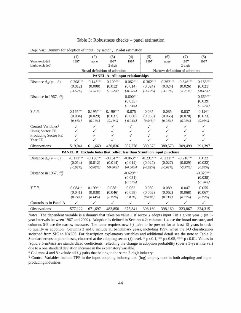
Table 3: Robustness checks – panel estimation
Dep. Var.: Dummy for adoption of inputi by sectorj; Probit estimation
(1) (2) (3) (4) (5) (6) (7) (8)Years excluded 1997 none 1997 1997 1997 none 1997 1997Links excluded‡ 2-digit 2-digit
Broad definition of adoption Narrow definition of adoptionPANEL A: All input relationships
Distancedij(y − 5) -0.208∗∗∗ -0.145∗∗∗ -0.199∗∗∗ -0.062∗∗∗ -0.362∗∗∗ -0.362∗∗∗ -0.346∗∗∗ -0.163∗∗∗
(0.012) (0.008) (0.012) (0.014) (0.024) (0.024) (0.026) (0.021)[-1.52%] [-1.51%] [-1.52%] [-0.36%] [-1.19%] [-1.19%] [-1.25%] [-0.47%]
Distance in 1967,d67ij -0.600∗∗∗ -0.669∗∗∗
(0.035) (0.039)[-1.64%] [-1.07%]
TFPi 0.165∗∗∗ 0.195∗∗∗ 0.190∗∗∗ -0.075 0.085 0.085 0.037 0.126∗
(0.034) (0.029) (0.037) (0.060) (0.065) (0.065) (0.070) (0.073)[0.14%] [0.21%] [0.16%] [-0.04%] [0.04%] [0.04%] [0.02%] [0.05%]
Control Variables§ X X X X X X X X
Using Sector FE X X X X X X X X
Producing Sector FE X X X X X X X X
Year FE X X X X X X X X
Observations 519,041 611,669 430,836 307,278 380,573 380,573 309,499 291,397
PANEL B: Exclude links that reflect less than $1million input purchase
Distancedij(y − 5) -0.173∗∗∗ -0.138∗∗∗ -0.161∗∗∗ -0.063∗∗∗ -0.231∗∗∗ -0.231∗∗∗ -0.210∗∗∗ 0.022(0.014) (0.012) (0.014) (0.014) (0.027) (0.027) (0.029) (0.022)[-0.92%] [-0.88%] [-0.86%] [-0.30%] [-0.62%] [-0.62%] [-0.57%] [0.05%]
Distance in 1967,d67ij -0.629∗∗∗ -0.829∗∗∗
(0.031) (0.038)[-1.67%] [-1.36%]
TFPi 0.084∗∗ 0.199∗∗∗ 0.088∗ 0.062 0.089 0.089 0.047 0.055(0.041) (0.038) (0.046) (0.058) (0.062) (0.062) (0.068) (0.067)[0.05%] [0.14%] [0.05%] [0.03%] [0.03%] [0.03%] [0.02%] [0.02%]
Controls as in Panel A X X X X X X X X
Observations 577,122 671,697 482,850 375,841 398,169 398,169 323,867 324,315
Notes: The dependent variable is a dummy that takes on value 1 if sector j adopts inputi in a given yeary (in 5-year intervals between 1967 and 2002). Adoption is defined inSection4.2; columns 1-4 use the broad measure, andcolumns 5-8 use the narrow measure. The latter requires newi-j pairs to be present for at least 15 years in orderto qualify as adoption. Columns 2 and 6 include all benchmarkyears, including 1997, when the I-O classificationswitched from SIC to NAICS. For description explanatory variables and additional detail see the note to Table2.Standard errors in parentheses, clustered at the adopting sector (j) level. * p<0.1, ** p<0.05, *** p<0.01. Values in[square brackets]are standardized coefficients, reflecting the change in adoption probability (over a 5-year interval)due to a one standard deviation increase in the explanatory variable.‡ Columns 4 and 8 exclude alli-j pairs that belong to the same 2-digit industry.§ Control Variables include TFP in the input-adopting industry, and (log) employment in both adopting and input-producing industries.
44

Table 4: Panel regressions with pairwise fixed effects
Dep. Var.: Dummy for adoption of inputi by sectorj in yeary
(1) (2) (3) (4) (5) (6)Remarks 2-digit† 1million‡ 2-digit 1million‡
Broad definition of adoption Narrow definition of adoptionDistancedij(y − 5) -0.0040∗∗∗ -0.0037∗∗∗ -0.0041∗∗∗ -0.0018∗∗∗ -0.0017∗∗∗ -0.0016∗∗∗
(0.0002) (0.0002) (0.0002) (0.0001) (0.0001) (0.0001)[-0.64%] [-0.59%] [-0.57%] [-0.28%] [-0.28%] [-0.22%]
TFPi 0.0034∗ 0.0029 -0.0107∗∗∗ 0.0002 -0.0003 -0.0040∗∗∗
(0.0019) (0.0019) (0.0015) (0.0008) (0.0007) (0.0006)[0.05%] [0.04%] [-0.16%] [0.00%] [-0.00%] [-0.06%]
Controls§ X X X X X X
Year FE X X X X X X
Pairwisei-j FE X X X X X X
Observations 556,936 523,627 568,771 555,529 522,718 566,600
Notes: All regressions are estimated by OLS. The dependent variable is a dummy that takes on value 1 if sectorjadopts inputi in a given yeary between 1972 and 2002. Bothi andj are observed at the 4-digit SIC level, and thepanel extends over the period 1967-2002 in 5-year intervals. Adoption is defined in Section4.2; columns 1-3 use thebroad measure, and columns 4-6 use the narrow measure. The latter requires newi-j links to remain intact for at least15 years in order to qualify as adoption. The table excludes adoptions occurring in 1997 because of the transition fromSIC to NAICS classification in that year. The main explanatory variable is network distance of inputi from sectorj inthe previous I-O benchmark year (i.e., with a 5-year lag), asdescribed in Section4.1. TFPi is the level of TFP in theinput-producing industry in yeary. Standard errors in parentheses, clustered at the adoptingsector (j) level. * p<0.1,** p<0.05, *** p<0.01. Values in[square brackets]are standardized coefficients, reflecting the change in adoptionprobability (over a 5-year interval) due to a one standard deviation increase in the explanatory variable.† Columns 2 and 5 exclude alli-j pairs that belong to the same 2-digit industry.‡ Columns 3 and 6 exclude links that reflect less than $1millioninput purchase.§ Controls include TFP in the input-adopting industry, and employment in both adopting and input-producing indus-tries.
45

Table 5: Panel results: Forward linkage distance
Dep. Var.: Dummy for adoption of inputi by sectorj in yeary
(1) (2) (3) (4) (5) (6)Links excluded‡ 2-digit 2-digit
Broad definition of adoption Narrow definition of adoptionForward Distancedji(y − 5) 0.010 0.010 0.027∗∗ -0.014 -0.015 0.015
(0.012) (0.012) (0.012) (0.013) (0.013) (0.012)[0.09%] [0.08%] [0.25%] [-0.08%] [-0.07%] [0.08]
Distancedij(y − 5) -0.213∗∗∗ -0.206∗∗∗ -0.361∗∗∗ -0.350∗∗∗
(0.012) (0.013) (0.024) (0.026)[-1.56%] [-1.56%] [-1.22%] [-1.29%]
Controls X X X X X X
Observations 488,947 488,947 406,865 358,171 358,171 292,034
Notes: The dependent variable is a dummy that takes on value 1 if sector j adopts inputi in a given yeary between1972 and 2002. All regressions are estimated by Probit. Controls are all those used in Table3, Panel A (includingall fixed effects). "Forward distancedji(y − 5)" is network distance (with a 5-year lag), using forward linkages fromsectorj to sectori, i.e., via other sectors thatj supplies to. For description of the remaining explanatory variablesand additional detail see the note to Table2. Standard errors in parentheses, clustered at the adoptingsector (j) level.* p<0.1, ** p<0.05, *** p<0.01. Values in[square brackets]are standardized coefficients, reflecting the change inadoption probability (over a 5-year interval) due to a one standard deviation increase in the explanatory variable.‡ Columns 3 and 6 exclude alli-j pairs that belong to the same 2-digit industry.
46
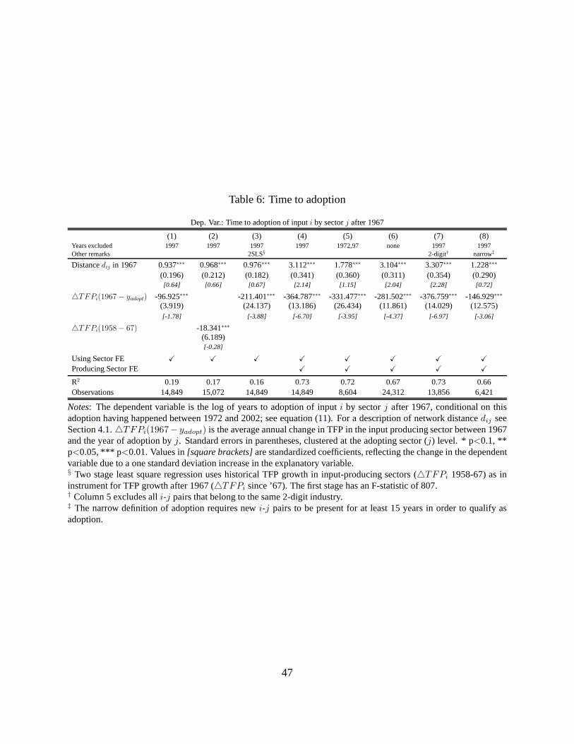
Table 6: Time to adoption
Dep. Var.: Time to adoption of inputi by sectorj after 1967
(1) (2) (3) (4) (5) (6) (7) (8)Years excluded 1997 1997 1997 1997 1972,97 none 1997 1997Other remarks 2SLS§ 2-digit† narrow‡
Distancedij in 1967 0.937∗∗∗ 0.968∗∗∗ 0.976∗∗∗ 3.112∗∗∗ 1.778∗∗∗ 3.104∗∗∗ 3.307∗∗∗ 1.228∗∗∗
(0.196) (0.212) (0.182) (0.341) (0.360) (0.311) (0.354) (0.290)[0.64] [0.66] [0.67] [2.14] [1.15] [2.04] [2.28] [0.72]
△TFPi(1967− yadopt) -96.925∗∗∗ -211.401∗∗∗ -364.787∗∗∗ -331.477∗∗∗ -281.502∗∗∗ -376.759∗∗∗ -146.929∗∗∗
(3.919) (24.137) (13.186) (26.434) (11.861) (14.029) (12.575)[-1.78] [-3.88] [-6.70] [-3.95] [-4.37] [-6.97] [-3.06]
△TFPi(1958− 67) -18.341∗∗∗
(6.189)[-0.28]
Using Sector FE X X X X X X X X
Producing Sector FE X X X X X
R2 0.19 0.17 0.16 0.73 0.72 0.67 0.73 0.66Observations 14,849 15,072 14,849 14,849 8,604 24,312 13,856 6,421
Notes: The dependent variable is the log of years to adoption of input i by sectorj after 1967, conditional on thisadoption having happened between 1972 and 2002; see equation (11). For a description of network distancedij seeSection4.1. △TFPi(1967− yadopt) is the average annual change in TFP in the input producing sector between 1967and the year of adoption byj. Standard errors in parentheses, clustered at the adoptingsector (j) level. * p<0.1, **p<0.05, *** p<0.01. Values in[square brackets]are standardized coefficients, reflecting the change in the dependentvariable due to a one standard deviation increase in the explanatory variable.§ Two stage least square regression uses historical TFP growth in input-producing sectors (△TFPi 1958-67) as ininstrument for TFP growth after 1967 (△TFPi since ’67). The first stage has an F-statistic of 807.† Column 5 excludes alli-j pairs that belong to the same 2-digit industry.‡ The narrow definition of adoption requires newi-j pairs to be present for at least 15 years in order to qualify asadoption.
47

Table 7: Firm level panel results
Dep. Var.: Dummy for firmj adopting inputs from firmi in a 5-year time intervaly
(1) (2) (3) (4) (5) (6) (7)OLS Probit OLS OLS OLS OLS OLS
Sample 2-digit† Manufacturing Services
Iij(y − 5) 0.02854∗∗∗ 1.61359∗∗∗ 0.02161∗∗∗ 0.02140∗∗ 0.01834∗∗ 0.01966∗∗ 0.02367∗
(0.00745) (0.11780) (0.00779) (0.00888) (0.00806) (0.00904) (0.01348)[2.85%] [2.69%] [2.16%] [2.14%] [1.83%] [1.97%] [2.37%]
ln(geodistance) -0.00006∗∗∗ -0.05809∗∗∗ -0.00007∗∗∗ -0.00007∗∗∗ -0.00006∗∗∗ -0.00006∗∗∗ -0.00007∗∗∗
(0.00001) (0.00604) (0.00001) (0.00001) (0.00001) (0.00002) (0.00001)[-0.007%] [-0.005%] [-0.007%] [-0.007%] [-0.006%] [-0.006%] [-0.007%]
△5 ln(Y/L)i 0.00003∗∗∗ 0.00003∗∗∗ 0.00003∗∗ 0.00003(0.00001) (0.00001) (0.00001) (0.00002)
Controls X X X X
Using Firm FE X X X X X
Producing Firm FE X X X X X
Year FE X X X X X X X
Observations 14,634,939 14,634,939 14,634,939 8,895,4818,461,685 4,906,536 3,381,959
Notes: The dependent variable is a dummy that takes on value 1 if firmj adopts inputi in a given 5-year intervalybetween 1977 and 2006.Iij(y − 5) is an indicator that equals one if firmsi andj were indirectly linked (had a binarydistance of 2) in the previous five-year interval. The variable geodistance is the geographical distance betweeni andj.△5 ln(Y/L)i denotes the change in output per worker in the input-producing firm (i) over the previous (lagged) 5-yearinterval. Controls include the change in output per worker in the input-using firm over the previous 5 year interval(△5 ln(Y/L)j), as well as output per worker and ln(employment) forbothinput-producing and input-using firms. Fora description of the firm-level dataset see Section6.1. Standard errors in parentheses, clustered at the adoptingfirm(j) level. * p<0.1, ** p<0.05, *** p<0.01. Values in[square brackets]are standardized coefficients. For the dummyIij(y − 5) (all other explanatory variables), these reflect the changein adoption probability due to an increase from 0to 1 (a one standard deviation increase in the explanatory variable).† Column 5 excludes alli-j pairs that belong to the same 2-digit SIC industry.
48

Online Appendix
Input Diffusion and the Evolution ofProduction Networks
Vasco M. Carvalho Nico VoigtländerCambridge and CEPR UCLA, NBER, and CEPR
A Proofs and Additional Detail on the Model
Proof of Proposition 2
Proof. We first derive the probability that the next variety to be classified into any sectorsj sources
as an input – indirectly, through its essential inputs – a given individual variety from sectorsi.
Recall from Definition1 thatµsj is the baseline vector that defines sectorsj . For example, for
a car these may be wheels, an engine, and a body. We will refer to an "ideal variety for sector
sj" as a variety that uses exactly the essential inputs inµsj . Next, letisj(≤ x) be the number of
positive entries in vectorµsj which in turn use varietyi as an input.1 Additionally, letksj be the
expected overlap between the next variety to be classified into sectorsj and the vectorµsj , i.e., the
expected number of varieties thatt has in common with the "ideal variety" for sectorsj . Then the
probability that the new variety in sectorsj sources fromi via its parents is:
pN
(ksj
isjxm
+(mK − ksj
) douti (t)
t
)mN
mKm(A.1)
wherem = pKmK + pNmN is the expected indegree for each variety (i.e., the expected number
of inputs). Sincet drawsmK essential inputs, there are overallmKm inputs in its network neigh-
borhood. Given thatt drawsmN varieties from this network, the termmN
mKmgives the probability
that it sources any given input via its network of essential inputs. Next, the term in parentheses in
(A.1) gives the probability that a given essential input sourcesfrom varietyi. This breaks down
into two parts. The first term in the parentheses accounts forthe possibility thati may be in the
network neighborhood of those essential inputs that classify t into sectorsj (i.e., inputs in the set
µsj ). The term gives the probability thatt will source fromi, conditional ont being classified into
sectorsj and sharing, in expectation,ksj essential inputs with the ideal variety defining sectorsj .
1In other words,isj (≤ x) is the number of links that lead from the essential varietiesdefining sectorj to varietyi.
Appendix p.1

The termisjxm
gives the probability of drawingi as a network input via these ideal varieties. In
expectation, the new variety will haveksj such draws. The second term accounts for the fact thatt
may also adopt inputi via essential inputs that are not in the setµsj , i.e., are not used to classifyt
as belonging tosj . This term gives the probability of drawingi as an input via the network, given
thatmK − ksj essential inputs are expected to be drawn uniformly at random from the population.
Finally, pN is the probability that inputi is actually adopted by the new variety given that it has
been discovered via its essential parents.
Now, according to our definition, each sector is a partition of the set of existent varieties. Hence,
the probability that sectorsj starts sourcing from sectorsi at t, conditional on not having done so
till t − 1 is the probability that the new varietyt selects as a network input any given variety in
sectorsi. This is obtained by summing the above expression over all varieties classified in sector
si:
∑
i′∈si
pN
(ksj
i′sjxm
+(mK − ksj
) douti′ (t)
t
)mN
mKm
= pN
(ksj∑
i′∈si
i′sjxm
+(mK − ksj
)∑
i′∈si
douti′ (t)
t
)mN
mKm
Finally, note thatksj = k for all sectorsj, i.e., the expected overlap of the new varietyt with any
sector’s ‘ideal’ list is the same across all sectors. This isimmediate from the joint assumption that
both ideal varieties defining a sector and the set of essential parents drawn by the new variety are
selected uniformly at random from the set oft− 1 existing varieties. Hence, the expression above
simplifies to:
pN
(k∑
i′∈si
i′sjxm
+ (mK − k)∑
i′∈si
douti′ (t)
t
)mN
mKm
For any two sectors,j and j′, this expression will only differ in the term∑
i′∈si
i′sjxm
. Hence if∑
i′∈sii′sj >
∑i′∈si
i′sj′ , thenj is more likely to adopt a variety in sectori thanj′. Now∑
i′∈sii′sj =
µ′sjνsi ≡ n(si,sj). Thus, ifsi is closer tosj than tosj′ at timet− 1, thensj is more likely to adopt
from si at timet, as claimed in the proposition.
Proof of Proposition 3
Proof. First, from the proof of Proposition2 recall that, ex-ante, the probability of any new variety
t being classified into a given sector is the same across sectors, and it is given by1/J . This follows
immediately from the joint assumption that both the ideal varieties defining sectors and the set of
essential inputs are drawn uniformly at random from the set of existing varieties. Therefore, the
Appendix p.2

number of varieties classified into sectorsi at timet, Ksi(t), is given by a Binomial distribution,
B(t, 1J).
Second, under the assumption of price symmetry, the sectoral (weighted) outdegree,woutsi
(t) at
time t, is proportional to the total number of varieties to which a sector sj supplies inputs at time
t, where the constant of proportionality is given by the priceφ.2 Thus
woutsi
(t) =
Ksi(t)∑
k=1
φdouti (t)
whereKsi(t) is the (random) number of varieties classified into sectorsi at timet.
Third, we are given that the variety-level outdegree,douti (t), is power law distributed. Notice
further that, sinceKsi(t) is distributed as a Binomial distribution, we have that:
Prob(Ksi(t) > x) = o(Prob(douti (t) > x)
that is,limx→∞Prob(Ksi
(t)>x)
Prob(douti >x)= 0. This is immediate from the fact that power law distributionsare
heavy-tailed while binomials are thin tailed.
Given the above observations, we can apply known results regarding the tail behavior of ran-
dom sums of power-law distributed variables. From Lemma 3.7.(1) in Jessen and Mikosch(2006,
p.8) we conclude that, asx → ∞
Prob(woutsi
(t) > x) ∼ φEt(Ksi(t))Prob(douti (t) > x) =φt
JProb(douti (t) > x)
That is, we have shown thatwoutsi
(t), the sectoral weighted outdegree of sectorsi, inherits
the outdegree tail behavior of the varieties classified intoit. Since all sectors are simply random
collections of varieties with the same outdegree distribution, this result holds true for every sector.
Therefore, we have shown that if the variety-level outdegree distribution at timet is power law, so
is the distribution of sectoral weighted outdegrees.
2The weighted outdegree refers to values of input flows, whileour variety-level predictions are based on binary(unweighted) input links. Because of price symmetry, product varietyj spends the same amount for each input varietyi that it uses (see the discussion at the end of Section3.2). Thus, the overallvalueof input varieties sold (outdegree)or used (indegree) by a sector is proportional to the underlying numberof input varieties.
Appendix p.3

mNm∗
N
Figure A.1: Optimal choice of network input adoption
Notes: The figure illustrates the optimal choice of input adoption. The x-axis shows the number of adopted networkinputs,mN . These are ranked by their customization cost as explained in Section3.2. The y-axis shows the term fromequation (8) that is proportional to marginal production cost, and thatan input adopter seeks to minimize. For smallmN , the input variety effect à laRomer(1990) dominates, so that production costs are decreasing if moreinputs areadopted. For highermN , customization costs for each additional adopted input arealso high, outweighing the inputvariety effect. Thus, production cost become increasing inmN . The optimal number of adopted network inputs isdenoted bym∗
N .
ReferencesJessen, A. and T. Mikosch (2006). Regularly Varying Functions. Publications de l’Institut Mathéma-
tique 80(94), 171–192.
Romer, P. M. (1990). Endogenous Technological Change.Journal of Political Economy 98(5), S71–S102.
Appendix p.4


![Stochastic Proximal Gradient Consensus Over Time-Varying ...people.ece.umn.edu/~mhong/DYSPGC.pdf · Convergence has been analyzed in many works [Nedic-Ozdaglar´ 09a][Nedic-Ozdaglar](https://img.pdfslide.us/doc/110x75/602f8cc36ffd6e250d14e69f/stochastic-proximal-gradient-consensus-over-time-varying-mhongdyspgcpdf.jpg)


![[PPT]Osmosis, Diffusion, Active Transport - Lake Shore … · Web viewOsmosis, Diffusion, Active Transport Diffusion, Osmosis and Concentration Gradient Diffusion – the movement](https://img.pdfslide.us/doc/110x75/5b257b6a7f8b9ae13b8b469c/pptosmosis-diffusion-active-transport-lake-shore-web-viewosmosis-diffusion.jpg)