Embed Size (px)
Citation preview
INORGANIC AND ORGANIC CARBON VARIATIONS IN SURFACE WATER, KONZA
PRAIRIE LTER SITE, USA, AND MAOLAN KARST EXPERIMENTAL SITE, CHINA
By
HUAN LIU
Submitted to the graduate degree program in Geology and the Graduate Faculty of the University
of Kansas in partial fulfillment of the requirements for the degree of Master of Science.
________________________________
Chairperson Gwendolyn L. Macpherson
________________________________
Luis González
________________________________
Jennifer Roberts
________________________________
Daniel Hirmas
________________________________
Randy Stotler
Date Defended: 27/01/2014
ii
The Thesis Committee for Huan Liu
certifies that this is the approved version of the following thesis:
INORGANIC AND ORGANIC CARBON VARIATIONS IN SURFACE WATER, KONZA
PRAIRIE LTER SITE, USA, AND MAOLAN KARST EXPERIMENTAL SITE, CHINA
________________________________
Chairperson Gwendolyn L. Macpherson
Date approved: 27/01/2014
iii
ABSTRACT
Two natural groundwater-fed streams were selected to examine the diurnal trends of
water geochemistry, CO2 emissions, and sources of OC on 25 May 2012 at the Konza Prairie
Long-Term Ecological Research (LTER) site, USA and 29 August – 30 August 2012 at the
Maolan Karst Experimental (Maolan) Site, China.
For the stream at the Konza LTER site, little variation in water chemistry was observed
among the upstream, midstream and downstream locations, indicating the groundwater and
stream water chemistry was mostly stable on a daily basis. 13
CDIC was the highest at the
downstream site due to the largest CO2 degassing. The autochthonous particulate organic carbon
(POC) fraction at the upstream, midstream and downstream sites was 12-35%, 39-65% and
75-88%, respectively. Estimation of the C/N ratio for POC samples at the three locations was
10.4-15.0, 14.0-15.9 and 12.2-13.3. This is comparable to previously measured C/N ratios of
suspended POC.
For the stream at the Maolan site, there was little or no diel variation in the spring water
physical and chemical parameters. However, all parameters show distinct diel changes in the
spring-fed midstream pond with flourishing submerged plants. Temperature, pH, DO, SIC,
13
CDIC increased during the day and decreased at night, while EC, [HCO3-], [Ca
2+], and pCO2
behaved in the opposite sense. Strong aquatic photosynthesis was indicated from maximum DO
values (two to three times higher than normal water equilibrated with atmospheric O2). In the
downstream pond with fewer submerged plants but larger volume, all parameters displayed
similar trends to the midstream pond but with much less change. We attribute this pattern to the
lower biomass/water volume ratio. The diel variations in the two ponds resulted from the aquatic
photosynthetic effect, demonstrating that natural surface water systems may constitute an
important sink of carbon.
iv
ACKNOWLEDGEMENTS
I would like to express my greatest appreciation to my scientific supervisor Dr.
Gwendolyn L. Macpherson for her patient guidance, and encouragement during my study at The
University of Kansas. I am inspired by her tremendous expertise, constant enthusiasm, rigorous
attitude towards academic research. The thesis could not have been completed without her
supervision and assistance.
I would also like to sincerely thank the University of Kansas geology faculty Dr. Luis
Gonzales, Dr. Jennifer Roberts, Dr. Daniel Hirmas, and Dr. Randy Stotler for valuable
instructions. I am very grateful to Greg Cane for his support with the lab work at KU and Dr.
Andrea Brookfield for taking the thermal images in the field at Konza.
Special thanks are given to Dr. Zaihua Liu for his thoughtful comments and suggestions,
which greatly improved the original Chapter 3 draft. Dr. Rui Yang, Dr. Hailong Sun and Chen Bo
are very much appreciated for their help in lab and field work in China.
This work was supported by the KU Department of Geology research grant, the Konza
Prairie LTER Program, and the 973 Program of China (2013CB956703).
v
TABLE OF CONTENTS
ABSTRACT……………………………………………………………………………………...iii
ACKNOWLEDGEMENTS………………………………………………………………………iv
CHAPTER 1. GENERAL INTRODUCTION……………………………………………………1
CHAPTER 2. SOURCES OF ORGANIC CARBON IN A STREAM, KONZA PRAIRIE
LONG-TERM ECOLOGICAL RESEARCH SITE, USA………………………………….…….4
Chapter summary……………………………………………………………………………...5
1. Introduction…………………………………………………………………………….......6
2. Settings……………………………………………………………………………………..7
3. Methods…………………………………………………………………………………….9
3.1. Field procedures………………………………………………………………………..9
3.2. Laboratory procedures………………………………………………………………..10
3.3. Calculations…………………………………………………………………………...11
4. Results………………………………………………………………………...…………...12
4.1. Physical chemistry of the stream water………………………………………………12
4.2. 13
C and C/N for the soil, plant and POC samples…………………………………...12
4.3. CO2 efflux.…………………………………………………………………...……….13
5. Discussion.…………………..…………………………………………...…………….….13
5.1. Physical chemistry of stream water.……………………..…………………………...13
5.1.1. Water temperature.……………………..………………………………………...13
5.1.2. PH.…………………………………………………………………...……….…..14
5.1.3. DO.…………………………………………………………………...……….….14
5.2. CO2 outgassing.…………………………………………………………………...…..14
5.3. Sources of DIC.…………………….…………………………………………….......16
vi
5.4. Calculation of POC sources from 13
C of plant, soil and POC samples.……….........16
5.5. Implication of estimated C/N of POC samples.……………………………………....18
6. Conclusions.…………………………………………………………………….…….......18
References.……………………………………………………………………….…….........20
CHAPTER 3. DIEL GEOCHEMICAL VARIATIONS IN A KARST SPRING AND TWO
PONDS, MAOLAN KARST EXPERIMENTAL SITE, CHINA…………………….……..…..37
Chapter summary.……………………...……………………………………………….........38
1. Introduction.……………………...……………………………………………….............40
2. Study area.……………………...…………………………………...…………………......41
3. Methods.……………………...…………………………………...………………….........42
3.1. Field monitoring and sampling.……………………...……...…………..………........42
3.2. Estimating CO2 partial pressure and the calcite saturation index.………………........43
3.3. Determining DIC and 13
CDIC.……………………...……...…………..……….........44
4. Results.…………………………………………………...……...…………..……….........45
4.1. Diel variations in physical chemistry and 13
CDIC.……………………...……...........45
4.1.1. Maolan spring.……………………...……...…………..……………...……........45
4.1.2. Midstream pond.……………………...……...……………………..………........45
4.1.3. Downstream pond.……………………...……...……………….…..………........46
4.2. CO2 flux.……………………………………………...……...…….……..……….......46
4.2.1. Maolan spring.……………………...……...………………...……..………........46
4.2.2. Midstream pond.……………………...................……...…………..………........47
4.2.3. Downstream pond.……………………...………….…...…………..………........47
5. Discussion.…………………………………...…………...……...…………..………........47
5.1. Mechanisms for DIC and 13
CDIC changes in the Maolan spring pool.…………...….47
vii
5.2. Mechanisms for diel variations in physical, chemical and isotopic properties of the
midstream pond.……………………...……...…………..……………………..........49
5.2.1. Groundwater input.……………………...……...…………..………………........49
5.2.2. Temperature.……………………...……...…………..…………………..…........50
5.2.3. Gas exchange between water and atmosphere.……………………...….……......50
5.2.4. Photosynthesis and respiration by submerged plants.……...………………........51
5.2.5. Calcite precipitation/ dissolution.……………………...…………...….…….......52
5.3. Mechanisms for diel variations in physical, chemical and isotopic properties of the
downstream pond.…………………………………...……...…………..………........53
5.4. Contribution of aquatic biological effects to the stability and sink of carbon….........53
5.4.1. Transformation of DIC into OC: organic carbon preservation potential.…….....53
5.4.2. CO2 influx from atmosphere to water: insight from the floating chamber
data in the midstream pond.………………………………...……...……….........54
5.4.3. Quantification of daily organic carbon formation in the two ponds.……….........55
6. Conclusions.……………………...……...…………………………..…..……….........56
References.……………………...……...…………..……………………………….........58
APPENDICIES.……………………...……...…………..………………………………….........73
Appendix A. Methods for Konza May sampling.……………………........……………........74
Sampling detail on 25 May.…………………………………….…........……………........74
Laboratory detail.……………………………………………….…........……………........75
Appendix B. Floating CO2 chamber.…………………………………….…........………......85
Appendix C. Long-term data analysis of Konza Prairie.……………………………….........87
Summary.…………………………………………………………….…........………......87
C.1. Introduction.…………………………………………………….…........………......87
viii
C.2. Study area.…………………………………………………….…...........………......89
C.2.1. Location.…………………………………………………….…........…….........89
C.2.2. Climate and vegetation.……………………………………….........………......90
C.2.3. Geology.………………………………………………………........………......91
C.2.4. Soils.…………………………………………………….….............………......92
C.2.5. Hydrogeology.……………………………………………………..….……......92
C.3. Methods.……………………………………..………………….…........………......93
C.3.1. Geochemical speciation modeling.……………….…………….....…..……......93
C.3.2. Other data.………………………………………………….…........………......94
C.3.3. Data analysis.…………………………………………………........…….…......94
C.4. Results.…………………………………………………….…........……………......95
C.4.1. Water chemistry.……………………………………………………...……......95
C.4.2. Atmospheric CO2.……………………………………………………….…......95
C.4.3. Long-term trends.……………………………………………………....…........96
C.4.4. Groundwater pCO2 in relation to other physical parameters.…………...…......96
C.4.5. Net primary production.………………………………………………………..97
C.5. Discussions.…………………………………………………….…........…….…......97
C.5.1. Implication from SPSS.…………………..……………….…........…….…......97
C.5.2. Controlling factors on groundwater pCO2.…………………………….…........98
C.5.2.1. Temperature and atmospheric pCO2.……………………........…….…......98
C.5.2.2. Prairie precipitation and Kings Creek discharge.…………………...…......99
C.5.3. Net primary production.…………………………………………………..…..100
C.6. Conclusions.…………………………………………………........………...…......101
Appendix D. Geochemical speciation modeling results from PHREEQC.……….….......109

ix
References cited in all appendices.……………………………………………………......110
1
CHAPTER 1. GENERAL INTRODUCTION
2
This master thesis is based on the field data collected on 25 May 2012 at the Konza
Prairie Long-Term Ecological Research (LTER) site, and 29 August – 30 August 2012 at the
Maolan Karst Experimental Site. Laboratory analyses were performed in the University of
Kansas and State Key Laboratory of Environmental Geochemistry facilities in cooperation with
the faculty and stuff of the Department of Geology and Chinese Academy of Science.
The purpose of this work was to incorporate measurements of the physical and chemical
parameters in groundwater-fed surface water to understand the underlying mechanisms causing
the daily differences. This work evaluates the contribution of dissolved inorganic carbon to
organic carbon and the CO2 gas exchange between water and atmosphere.
Chapter 2 and 3 describe slightly different focuses on the similar aspect of the thesis
work in two natural carbonate terrains. Each of the two chapters contains a summary,
introduction, location, methods, results, discussion, and conclusions. The appendices provide
more details about the sampling, methods and additional information and data not included in
those chapters. The long-term data analysis of groundwater geochemistry at Konza Prairie is also
in the appendices.
Chapter 2 discusses the processes influencing CO2 emissions from a 5th
-order
groundwater-fed stream at the Konza Prairie LTER site, USA. Direct CO2 outgassing rate from
the stream water is measured using the floating chamber approach. The measured fluxes are
compared with fluxes calculated from the lake gas transfer velocity. Thermal imaging is used to
verify that groundwater is discharged to the stream. The fluxes are also used to estimate the
fraction of transformation of dissolved inorganic carbon (DIC) into organic carbon using stable
carbon isotopes; the C/N ratio of POC, calculated using the same fraction, is compared to
previously measured POC, and so is an independent verification of the calculations.
3
Chapter 3 reveals the underlying mechanisms of diel spatiotemporal differences in
groundwater-fed ponds at the Maolan Karst Experimental Site, China. It characterizes the water
geochemistry and stable carbon isotopes in three ponds. The dominating factors (including
groundwater input, water temperature, gas exchange, biological processes and calcite
dissolution/precipitation) controlling the daily spatiotemporal variations are proposed. CO2
efflux/influx is examined using the floating chamber approach. The daily organic carbon
formation is quantified.
Inland freshwater ecosystems are parts of the terrestrial landscape, but they have not yet
been included in the terrestrial greenhouse gas balance. This study shows reasons to consider
groundwater and surface water as one of the missing carbon sinks in the global carbon budget
and provides a valuable tool for improving input to quantification of the global carbon cycle.
4
CHAPTER 2. SOURCES OF ORGANIC CARBON IN A STREAM, KONZA PRAIRIE
LONG-TERM ECOLOGICAL RESEARCH SITE, USA
5
Chapter summary
Inland freshwater ecosystems (mainly rivers, lakes, and reservoirs) play a significant role
in the global and regional carbon cycle because organic carbon (OC) formed during aquatic
photosynthesis incorporates dissolved inorganic carbon (DIC). DIC may be sourced from
chemical weathering of carbonates; thus, carbonates may play a role in sequestration of
atmospheric or groundwater CO2 in the long run. In this study, a tributary stream in a
carbonate-rich terrain at the Konza Long-Term Ecological Research (LTER) site, USA, was
selected to study the sources and dynamics of DIC and OC.
Water samples and CO2 samples were taken at three locations from upstream to
downstream on 25 May under cloudy/sunny weather. The stream water level was lower than the
mean daily statistic. Infrared images show colder groundwater discharging into warmer stream
water from the stream channel side and bottom at all three locations. The pH ranged from 7.1 to
7.4. The temperature of downstream location was the highest (19.9oC). DO ranged from 4.7
mg/L (upstream) to 6.1 mg/L (downstream). DO% was highest at the downstream site. 13
CDIC
was the highest at the downstream site and resulted from the largest CO2 outgassing. There was
little variation in the other parameters among the three locations indicating the groundwater and
stream water chemistry was mostly stable during midday.
13
C of soil samples, POC samples, aquatic and terrestrial plant samples were determined
in order to calculate the autochthonous fraction. The estimated percentage of autochthonous
carbon in POC at the upstream, midstream and downstream sites is 12-35%, 39-65% and 75-88%,
respectively. However, the overall aquatic photosynthesis at Konza was not strong due to the
lack of submerged plants, also evidenced by low DO.
6
1. Introduction
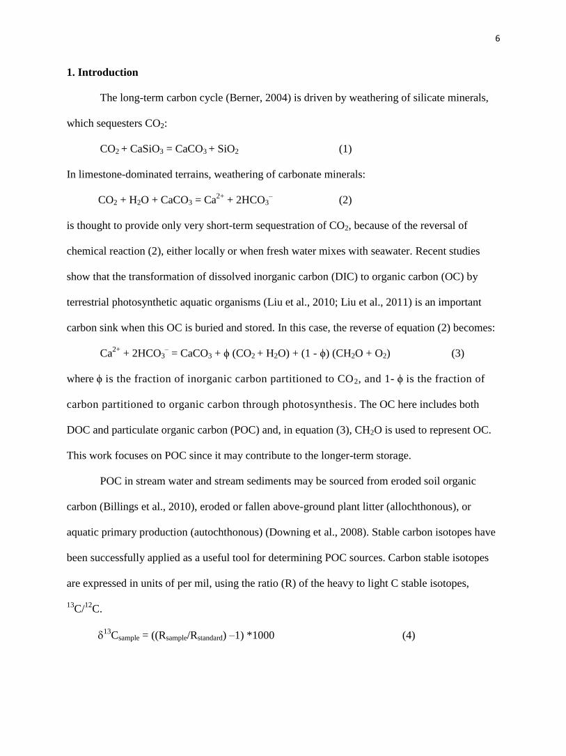
The long-term carbon cycle (Berner, 2004) is driven by weathering of silicate minerals,
which sequesters CO2:
CO2 + CaSiO3 = CaCO3 + SiO2 (1)
In limestone-dominated terrains, weathering of carbonate minerals:
CO2 + H2O + CaCO3 = Ca2+
+ 2HCO3– (2)
is thought to provide only very short-term sequestration of CO2, because of the reversal of
chemical reaction (2), either locally or when fresh water mixes with seawater. Recent studies
show that the transformation of dissolved inorganic carbon (DIC) to organic carbon (OC) by
terrestrial photosynthetic aquatic organisms (Liu et al., 2010; Liu et al., 2011) is an important
carbon sink when this OC is buried and stored. In this case, the reverse of equation (2) becomes:
Ca2+
+ 2HCO3– = CaCO3 + ϕ (CO2 + H2O) + (1 - ϕ) (CH2O + O2) (3)
where ϕ is the fraction of inorganic carbon partitioned to CO2, and 1- ϕ is the fraction of
carbon partitioned to organic carbon through photosynthesis. The OC here includes both
DOC and particulate organic carbon (POC) and, in equation (3), CH2O is used to represent OC.
This work focuses on POC since it may contribute to the longer-term storage.
POC in stream water and stream sediments may be sourced from eroded soil organic
carbon (Billings et al., 2010), eroded or fallen above-ground plant litter (allochthonous), or
aquatic primary production (autochthonous) (Downing et al., 2008). Stable carbon isotopes have
been successfully applied as a useful tool for determining POC sources. Carbon stable isotopes
are expressed in units of per mil, using the ratio (R) of the heavy to light C stable isotopes,
13C/
12C.
13
Csample = ((Rsample/Rstandard) –1) *1000 (4)
7
Aquatic plants are generally enriched in 12
C when compared with terrestrial plants due to
different fractionation mechanisms (Mook and Tan, 1991). Terrestrial C4 plants have higher
carbon isotope ratios than C3 plants (Farquhar et al., 1982). Therefore, the 13
C of POC can
potentially differentiate between C sourced from aquatic plants, terrestrial plants, soils and/or
groundwater. However, if the carbon isotope composition of different carbon pools overlap with
each other, an additional discriminant, such as C/N ratio (Tao et al., 2009; Sun et al., 2011), can
be used in conjunction with carbon isotope ratios.
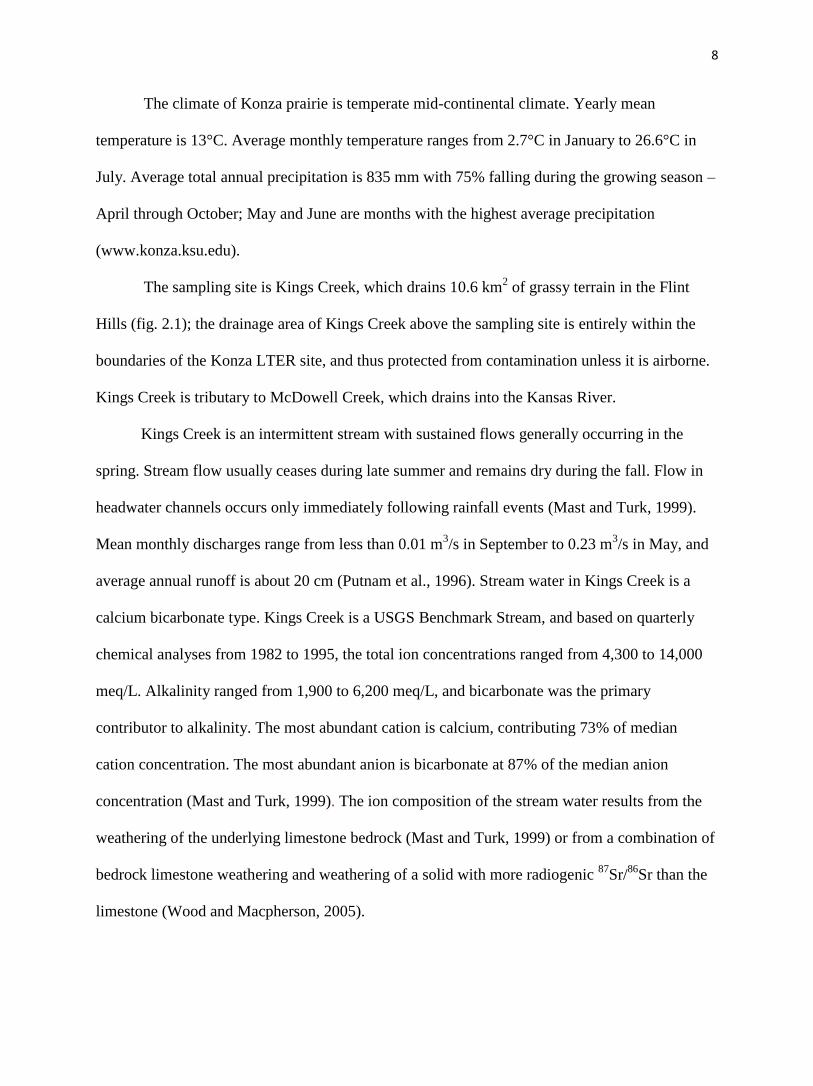
2. Setting
The Konza Long Term Ecological Research Site (Konza) is a 3487 ha tallgrass prairie
located in the Flint Hills region of northeastern Kansas, about 10 km south of Manhattan,
Kansas. The Flint Hills region encompasses over 1.6 million ha extending throughout much of
eastern Kansas from near the Kansas-Nebraska border south into northeastern Oklahoma, and
contains the largest remaining area of unplowed tallgrass prairie in North America. Konza is an
unplowed native tallgrass prairie. The vegetation is mostly perennial, warm-season C4 grasses,
predominately big bluestem, little bluestem, Indiangrass and switchgrass. Less abundant species
include warm-season and cool-season grasses, composites, legumes, and other forbs. Riparian
zones are mostly wooded in lower stream reaches and prairie in the uppermost stream reaches
(www.konza.ksu.edu).
The bedrock at Konza is composed of Early Permian couplets of limestone and shale.
The 1 – 2 m thick limestone layers and the alluvial deposits act as aquifers at this site. Konza
prairie soils are developed on loess, limestone and shale, and are generally less than 1 m thick
(Macpherson et al., 2008). Soils are usually carbonate-poor, with moderate to low cation
exchange capacities (mostly < 40 cmolc/kg) (Ransom et al., 1998).
8
The climate of Konza prairie is temperate mid-continental climate. Yearly mean
temperature is 13°C. Average monthly temperature ranges from 2.7°C in January to 26.6°C in
July. Average total annual precipitation is 835 mm with 75% falling during the growing season –
April through October; May and June are months with the highest average precipitation
(www.konza.ksu.edu).
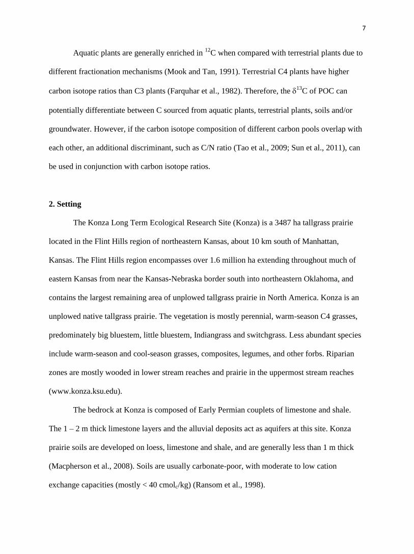
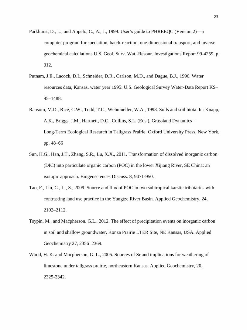
The sampling site is Kings Creek, which drains 10.6 km2 of grassy terrain in the Flint
Hills (fig. 2.1); the drainage area of Kings Creek above the sampling site is entirely within the
boundaries of the Konza LTER site, and thus protected from contamination unless it is airborne.
Kings Creek is tributary to McDowell Creek, which drains into the Kansas River.
Kings Creek is an intermittent stream with sustained flows generally occurring in the
spring. Stream flow usually ceases during late summer and remains dry during the fall. Flow in
headwater channels occurs only immediately following rainfall events (Mast and Turk, 1999).
Mean monthly discharges range from less than 0.01 m3/s in September to 0.23 m
3/s in May, and
average annual runoff is about 20 cm (Putnam et al., 1996). Stream water in Kings Creek is a
calcium bicarbonate type. Kings Creek is a USGS Benchmark Stream, and based on quarterly
chemical analyses from 1982 to 1995, the total ion concentrations ranged from 4,300 to 14,000
meq/L. Alkalinity ranged from 1,900 to 6,200 meq/L, and bicarbonate was the primary
contributor to alkalinity. The most abundant cation is calcium, contributing 73% of median
cation concentration. The most abundant anion is bicarbonate at 87% of the median anion
concentration (Mast and Turk, 1999). The ion composition of the stream water results from the
weathering of the underlying limestone bedrock (Mast and Turk, 1999) or from a combination of
bedrock limestone weathering and weathering of a solid with more radiogenic 87
Sr/86
Sr than the
limestone (Wood and Macpherson, 2005).
9
3. Methods
3.1. Field Procedures
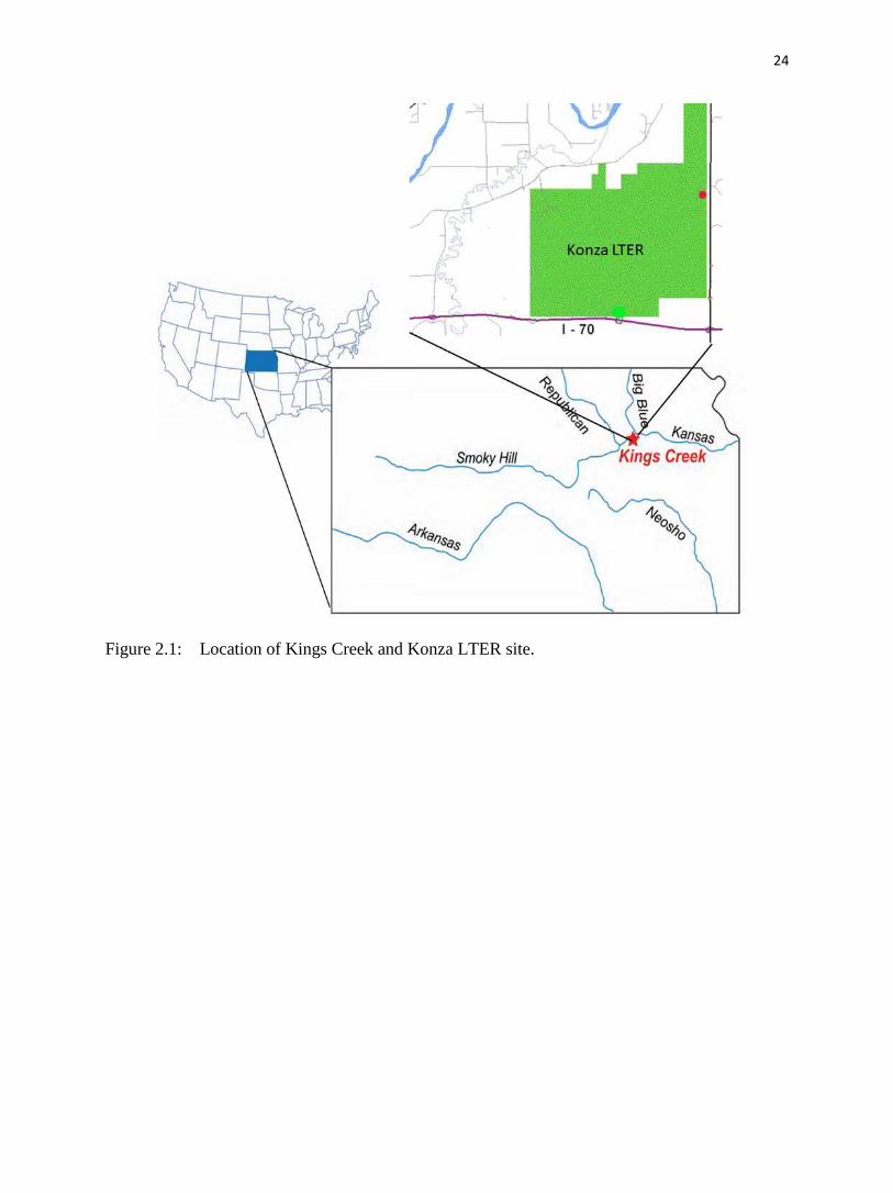
The field sampling occurred on 25 May 2012. This is normally the wet season of the year,
but 2012 was exceptional in that the discharge rate of Kings Creek was about 56.6 L/s lower than
the median daily statistic of 33 years (fig. 2.2). We collected water samples from three locations
on Kings Creek, here called upstream, midstream and downstream. Based on the GPS
coordinates, the distance between upstream and midstream locations is about 22 m, and about 26
m between midstream and downstream locations. At each sampling location, water in the center
of the stream was collected 5 cm above the bottom for parts deeper than 10 cm and near the
bottom for parts shallower than 10 cm. Samples for C/N of POC and 13
CPOC were each collected
into two pre-cleaned 2 L HDPE bottles and poisoned with saturated HgCl2 immediately after
collection. On that day, these water samples were filtered through pre-weighted, pre-ashed
(500°C, 5h) 47 mm Whatman GF/F glass fiber filters (0.65 µm). A two-liter sample in a
pre-cleaned HDPE temporary collection bottle was placed immediately on ice, and filtered in the
field-station laboratory through 0.45 µm filters into three containers. The first was a pre-cleaned
30-mL glass vial for determination of 13
CDIC that was filled from the bottom until there was no
air space. The next two were pre-cleaned 250 mL LDPE bottles. One of the two 250 mL bottles
was filled so no air space remained and used for anion determination, including alkalinity. The
other, pre-weighed, was filled to approximately 250 mL, weighed in the lab, and concentrated
nitric acid added at a volume proportion of 1:50 (acid:sample) for preservation of cations. All
liquid samples were stored in a cold environment (4oC) until analyzed.
Samples for terrestrial (vegetation and soil) and aquatic carbon were collected for 13
C
and C/N content. At each site, leaves from 10 land plant samples were collected for 13
C analysis
and used to approximate the 13
C of terrestrial C3 and C4 plants. The previously measured OC
10
13
C at Konza (Johnson et al., 2007) would serve as a test of the validity of this approximation.
Three soil samples from each site (from 0~45 cm depth) were collected using a shallow depth
Backsaver® soil sampler to establish a representative C/N and 13
C for soil organic matter.
Three samples of submerged aquatic plants were collected and analyzed to establish the aquatic
isotopic signature of 13
C.
Unstable parameters (pH; temperature; dissolved oxygen, DO; Eh) were measured on site
in a beaker using individual probes and meters.
A floating CO2 chamber was placed on the surface of the waters to collect CO2 efflux
from the stream (details in section 4.c, below). Five CO2 samples were taken at an interval of
approximately 1-min at each location.
3.2. Laboratory Procedures
Sample treatment: The glass-fiber filters were freeze-dried for POC, C/N and 13
C
analyses. They were then acidified with dilute HCl and oven-dried overnight at 105°C and
weighed prior to analysis. A portion of the filter paper was cut and loaded into a 9 x 10 mm tin
capsule. Terrestrial and aquatic plant samples were washed under DI water to get rid of dust/soil;
oven-dried for 2-3 days at 46oC and grinded using a mortar and pestle with liquid nitrogen added.
Roots in the soil samples were picked out and soil samples were dried overnight and weighted;
acidified with 0.5 M HCl.
Laboratory analyses: The C/N content and 13
C was determined on a Costech ECS 4010
elemental analyzer and a dual-inlet isotope ratio mass spectrometer (ThermoFinnigan MAT 253
Dual Inlet System), respectively at the W. M. Keck Paleoenvironmental and Environmental
Stable Isotope Laboratory (Dept. of Geology). Alkalinity was determined by titration with ~0.02
N H2SO4, with the titration end point determined as the maximum slope of the titration curve in
11
the vicinity of pH 4.5. Other major anion concentrations (Cl, NO3-N, SO4) were determined by
ion chromatography (KU Aqueous Geochemistry Lab, Dept. of Geology). Cation concentrations
(Ca, Mg, Na, K, Sr, B, Ba, Li, Si, F) were determined by ICP-OES (KU Plasma Analytical
Laboratory, Dept. of Geology).
3.3. Calculations
The fraction of autochthonous and allochthonous POC can be quantified by considering
their 13
C values as end-members in a mass balance:
13Csample=X*
13Cau + (1-X)*
13Cal (5)
(C/N)sample=Y*(C/N)au + (1-Y)*(C/N)al (6)
In these equations, “au” is subscript for autochthonous and “al” is subscript for
allochthonous. The data from POC in stream waters will be used for 13
Csample. X and Y are the
fraction of the autochthonous POC calculated from (5) and (6) based on 13
C and C/N. 1-X and
1-Y are the fractions of allochthonous POC. Theoretically, for the proportion of autochthonous
POC, X = Y, and for the proportion of allochthonous POC, 1-X = 1-Y.
DIC, calcite saturation and pCO2 were calculated using the geochemical speciation model
PHREEQC Interactive 2.18.5570, with the PHREEQC database (Parkhurst and Appelo, 1999.)
Precise pH measurements are critical for determining carbonate system equilibria (Langmuir,
1971). We used field-measured pH and temperature along with laboratory-determined alkalinity
(prior work at this site shows alkalinity in filtered, cooled samples does not change for at least
two weeks after sample collection; Macpherson, unpublished data), other anions, and cations.
The excellent charge balances on the samples collected (-0.00031~ -0.00029) support use of
laboratory-determined measurements.
12
4. Results
4.1. Physical chemistry of the stream water
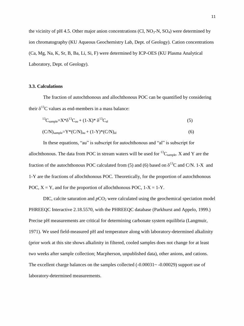
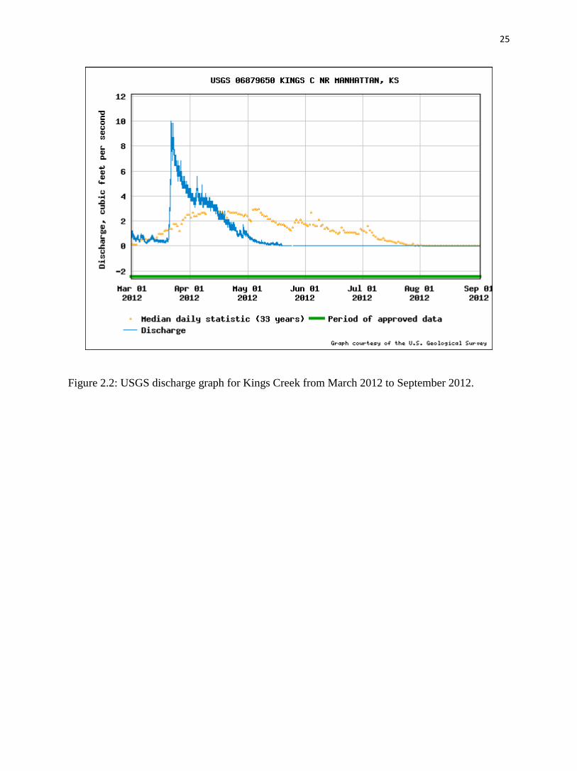
Fig. 2.3 shows colder groundwater discharging into warmer stream water from the side
and bottom of the stream channel. From the infrared image (fig. 2.3a) that was taken from a
position near the midstream location, the groundwater temperature was around 18.3°C at the time
the image was captured. Table 2.1 shows the physical chemistry of the upstream, midstream and
downstream water, sampled in that order. The temperature of the downstream-site water was the
highest (19.9°C); the air temperature also increased during the sampling from 21°C to 23°C over
the entire sampling day. DO ranged from 4.7 mg/L at the upstream site to 6.1 mg/L at the
downstream site. The DO% was also the highest at the downstream site. 13
CDIC was highest at
the downstream site and lowest at the midstream site. There was little variation in the other
parameters among the three locations. The pH ranged from 7.1 to 7.4, SC varied from 637 µs/cm
to 643 µs/cm, averaging 640 µs/cm. Eh changed from 194 mv to 198 mv. The alkalinity, at an
average of 383 mg/L, is typical of water in limestone aquifers. Calculated CO2 values from
PHREEQC for the upstream, middle and downstream sites were 16800 ppmv, 26800 ppmv and
13400 ppmv, respectively.
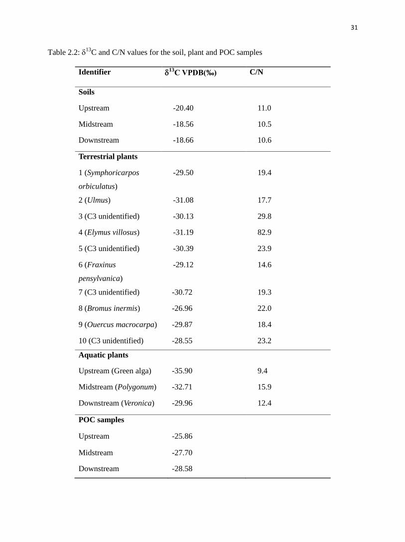
4.2. 13
C and C/N for the soil, plant and POC samples
Table 2.2 shows that 13
C and C/N of soil samples ranged from -20.40‰ to -18.56‰,
and 10.5 to 11.0, respectively. 13
C and C/N of terrestrial plant samples ranged from -31.19‰ to
-26.96‰, and 14.6 to 82.9. 13
C and C/N of aquatic plant samples ranged from -35.90‰ to
-29.96‰, and 9.4 to 15.9. 13
C of POC samples was the lowest at downstream site (-28.58‰)
and highest at upstream (-25.86‰). The C/N values of POC samples could not be measured
because of the low N content.
13
4.3. CO2 efflux
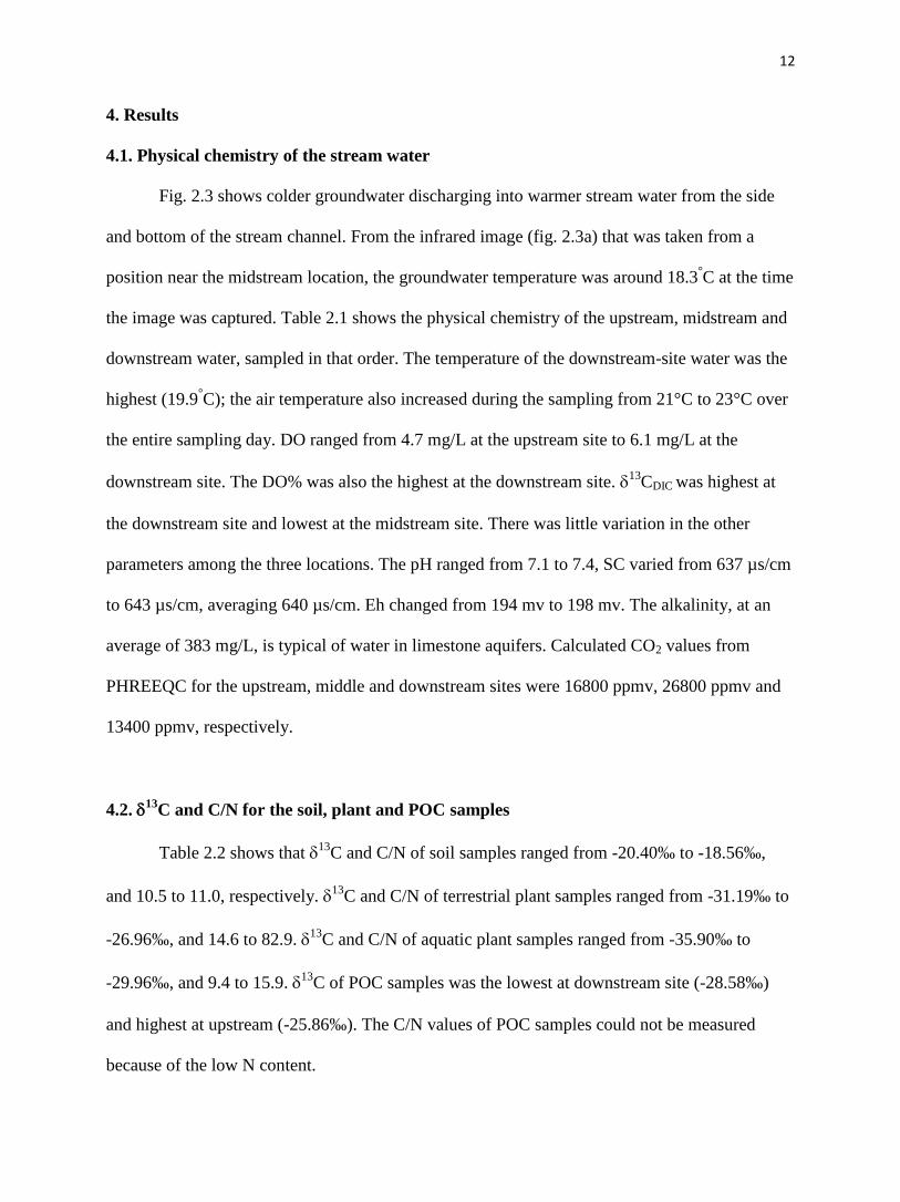
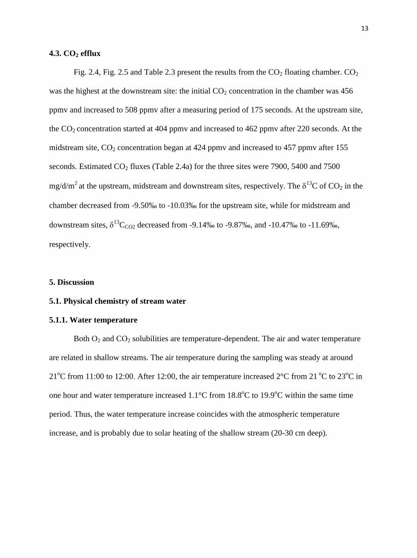
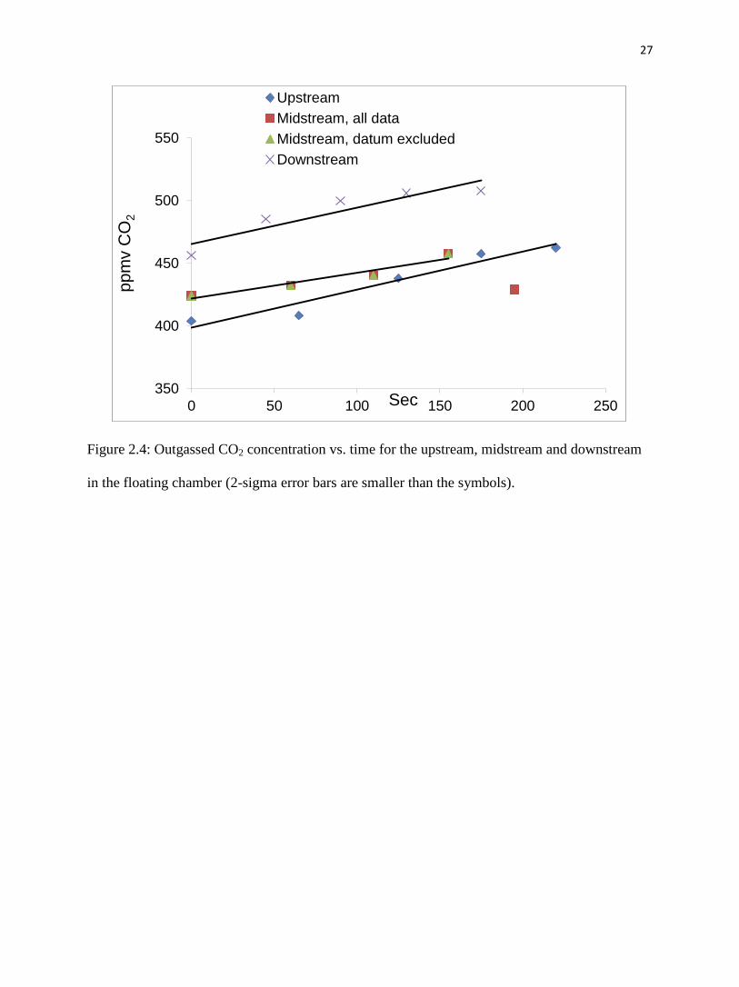
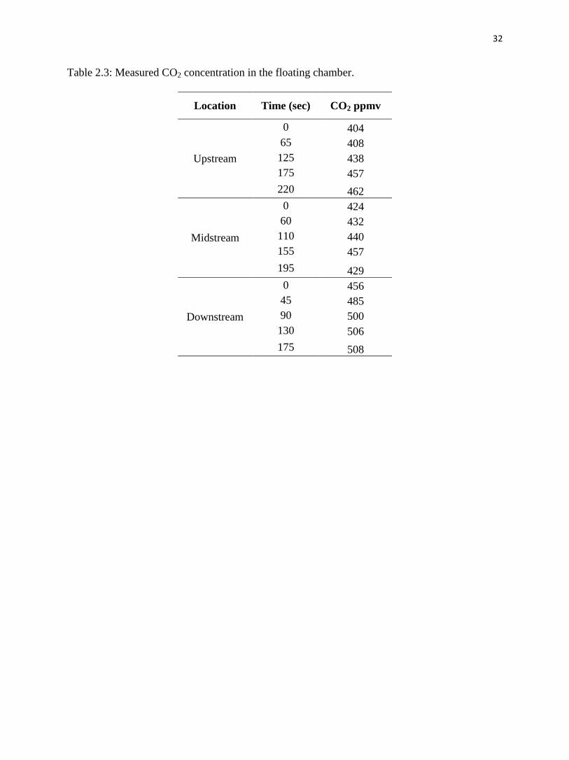
Fig. 2.4, Fig. 2.5 and Table 2.3 present the results from the CO2 floating chamber. CO2
was the highest at the downstream site: the initial CO2 concentration in the chamber was 456
ppmv and increased to 508 ppmv after a measuring period of 175 seconds. At the upstream site,
the CO2 concentration started at 404 ppmv and increased to 462 ppmv after 220 seconds. At the
midstream site, CO2 concentration began at 424 ppmv and increased to 457 ppmv after 155
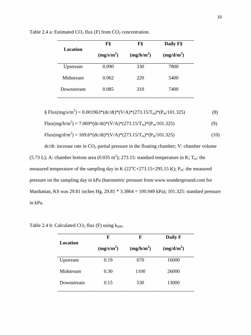
seconds. Estimated CO2 fluxes (Table 2.4a) for the three sites were 7900, 5400 and 7500
mg/d/m2
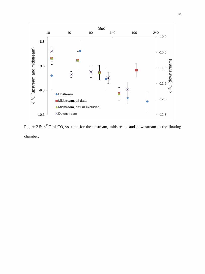
at the upstream, midstream and downstream sites, respectively. The 13
C of CO2 in the
chamber decreased from -9.50‰ to -10.03‰ for the upstream site, while for midstream and
downstream sites, 13
CCO2 decreased from -9.14‰ to -9.87‰, and -10.47‰ to -11.69‰,
respectively.
5. Discussion
5.1. Physical chemistry of stream water
5.1.1. Water temperature
Both O2 and CO2 solubilities are temperature-dependent. The air and water temperature
are related in shallow streams. The air temperature during the sampling was steady at around
21oC from 11:00 to 12:00. After 12:00, the air temperature increased 2°C from 21
oC to 23
oC in
one hour and water temperature increased 1.1°C from 18.8oC to 19.9
oC within the same time
period. Thus, the water temperature increase coincides with the atmospheric temperature
increase, and is probably due to solar heating of the shallow stream (20-30 cm deep).
14
5.1.2. pH
The pH ranged from 7.1 to 7.4 from upstream site to downstream site. The water
temperature difference (1.1 oC) was not enough to result in a change of 0.3 pH units. The
relatively high alkalinity (average 383 mg/L) in the streams means that the pH is regulated by the
CO2 levels in the water (Neal et al., 2002), i.e., as the pCO2 increases, pH decreases. The pCO2
for the downstream is the lowest, thus, pH is the highest.
5.1.3. DO
Solubility of O2 is temperature-dependent: higher water temperature lowers gas solubility.
At the sampled sites, the highest DO and DO% was 6.1 mg/L and 65% at 13:00 when stream
temperature was also the highest (19.9 oC). We propose that aquatic photosynthesis producing O2
was greater than the temperature effect that should have reduced the DO at the downstream
location. Nevertheless, the highest DO was still lower than water equilibrated with atmospheric
O2 (~9 mg/L at 20oC). This suggests that aquatic photosynthesis was active but not active enough
to produce more oxygen in the stream than is provided by the groundwater baseflow or
consumed by respiration, a conclusion corroborated by the observation of the scarcity of aquatic
plants living in the stream.
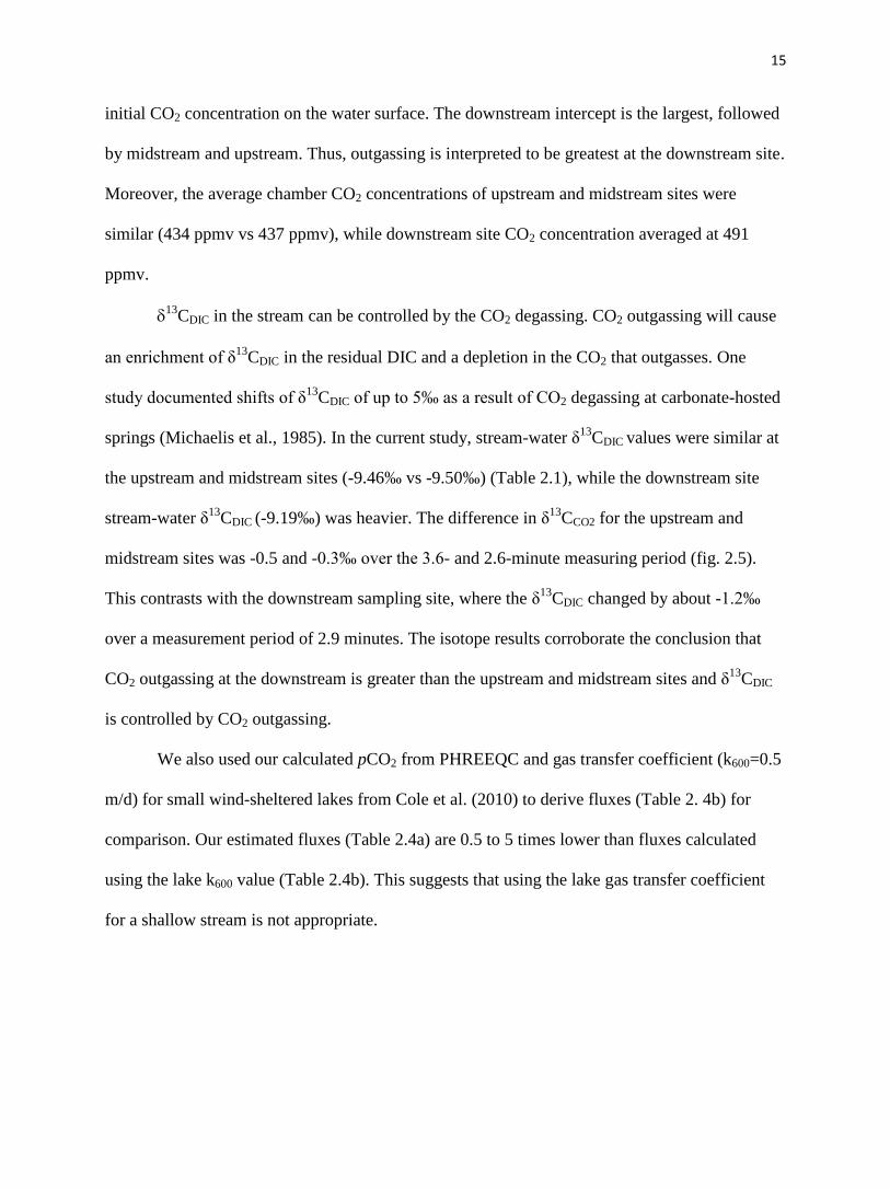
5.2. CO2 outgassing
Streamwater tends to be supersaturated with CO2, that is, out of equilibrium with
atmosphere (Butman and Raymond, 2011). The atmospheric CO2 mixing ratio was around 394
ppmv at the time of sampling. CO2 measured in the floating chamber at all three sites ranged
from 404 ppmv to 508 ppmv and averaged 454 ppmv (fig. 2.4). This is about 15% higher than
the atmospheric CO2 value, indicating CO2 outgassing. The intercepts of the lines reflect the
15
initial CO2 concentration on the water surface. The downstream intercept is the largest, followed
by midstream and upstream. Thus, outgassing is interpreted to be greatest at the downstream site.
Moreover, the average chamber CO2 concentrations of upstream and midstream sites were
similar (434 ppmv vs 437 ppmv), while downstream site CO2 concentration averaged at 491
ppmv.
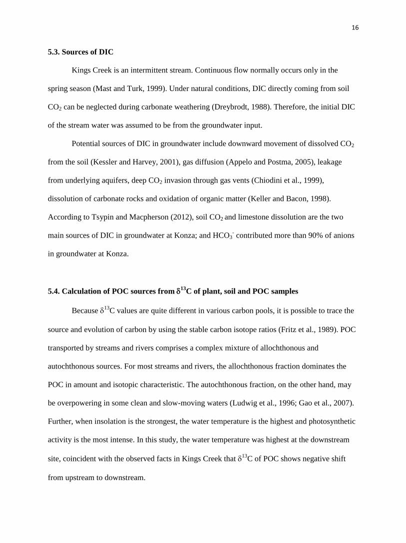
13
CDIC in the stream can be controlled by the CO2 degassing. CO2 outgassing will cause
an enrichment of δ13
CDIC in the residual DIC and a depletion in the CO2 that outgasses. One
study documented shifts of δ13
CDIC of up to 5‰ as a result of CO2 degassing at carbonate-hosted
springs (Michaelis et al., 1985). In the current study, stream-water δ13
CDIC values were similar at
the upstream and midstream sites (-9.46‰ vs -9.50‰) (Table 2.1), while the downstream site
stream-water δ13
CDIC (-9.19‰) was heavier. The difference in δ13
CCO2 for the upstream and
midstream sites was -0.5 and -0.3‰ over the 3.6- and 2.6-minute measuring period (fig. 2.5).
This contrasts with the downstream sampling site, where the δ13
CDIC changed by about -1.2‰
over a measurement period of 2.9 minutes. The isotope results corroborate the conclusion that
CO2 outgassing at the downstream is greater than the upstream and midstream sites and δ13
CDIC
is controlled by CO2 outgassing.
We also used our calculated pCO2 from PHREEQC and gas transfer coefficient (k600=0.5
m/d) for small wind-sheltered lakes from Cole et al. (2010) to derive fluxes (Table 2. 4b) for
comparison. Our estimated fluxes (Table 2.4a) are 0.5 to 5 times lower than fluxes calculated
using the lake k600 value (Table 2.4b). This suggests that using the lake gas transfer coefficient
for a shallow stream is not appropriate.
16
5.3. Sources of DIC
Kings Creek is an intermittent stream. Continuous flow normally occurs only in the
spring season (Mast and Turk, 1999). Under natural conditions, DIC directly coming from soil
CO2 can be neglected during carbonate weathering (Dreybrodt, 1988). Therefore, the initial DIC
of the stream water was assumed to be from the groundwater input.
Potential sources of DIC in groundwater include downward movement of dissolved CO2
from the soil (Kessler and Harvey, 2001), gas diffusion (Appelo and Postma, 2005), leakage
from underlying aquifers, deep CO2 invasion through gas vents (Chiodini et al., 1999),
dissolution of carbonate rocks and oxidation of organic matter (Keller and Bacon, 1998).
According to Tsypin and Macpherson (2012), soil CO2 and limestone dissolution are the two
main sources of DIC in groundwater at Konza; and HCO3- contributed more than 90% of anions
in groundwater at Konza.
5.4. Calculation of POC sources from 13
C of plant, soil and POC samples
Because 13
C values are quite different in various carbon pools, it is possible to trace the
source and evolution of carbon by using the stable carbon isotope ratios (Fritz et al., 1989). POC
transported by streams and rivers comprises a complex mixture of allochthonous and
autochthonous sources. For most streams and rivers, the allochthonous fraction dominates the
POC in amount and isotopic characteristic. The autochthonous fraction, on the other hand, may
be overpowering in some clean and slow-moving waters (Ludwig et al., 1996; Gao et al., 2007).
Further, when insolation is the strongest, the water temperature is the highest and photosynthetic
activity is the most intense. In this study, the water temperature was highest at the downstream
site, coincident with the observed facts in Kings Creek that 13
C of POC shows negative shift
from upstream to downstream.
17
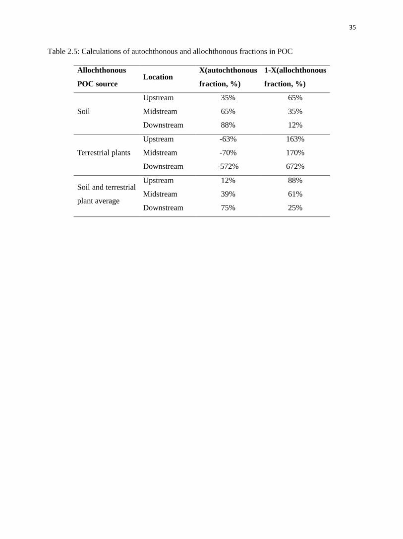
Although allochthonous POC in stream derives from soil and terrestrial plants, it is
necessary to delimit the upper and lower limits of allochthonous POC fraction using soil and
terrestrial plants 13
C separately. Calculated allochthonous POC percentage using soil as an end
member for the upstream, midstream and downstream sites is about 65%, 35% and 12%,
respectively (Table 2.5). However, using terrestrial plants 13
C as an end member for
allochthonous POC resulted in negative values of the calculated autochthonous fraction, which is
unrealistic. Therefore, the allochthonous POC portion cannot originate entirely from land plants
and at least part of it should come from the soil. Calculated allochthonous POC fraction using the
average soil and terrestrial plants 13
C for the upstream, midstream and downstream sites is
about 88%, 61% and 25%, respectively. The fallem tree leaves in Kings Creek lose 90% of their
material between 91 to 1439 days (Gray and Dodds, 1998). Based on observations, all the
particles on the filter paper were relatively small suggesting the leaf and root particles from land
plants might be neglected. Thus, a larger part of the allochthonous POC in the water should be
derived from soil.
Calculations based on the 13
C show that the contribution of groundwater-sourced carbon
to autochthonous POC at the upstream, midstream and downstream sites, based on using soil
alone or soil plus plants as the allochthonous end member, is 12-35%, 39-65% and 75-88%,
respectively. The downstream site showed the highest contribution from groundwater carbon in
POC, suggesting the strongest aquatic photosynthetic effect among the three sites. From equation
(3), an independent indicator of photosynthesis, DO showed synchronous change with water
temperature. When the sunlight was strong at 13:00, water temperature increased, aquatic plants
used DIC and the energy from the sunlight to produce O2. Therefore, the DO and DO% were
both the highest in the downstream location and alkalinity was the lowest, although the alkalinity
change was small.
18
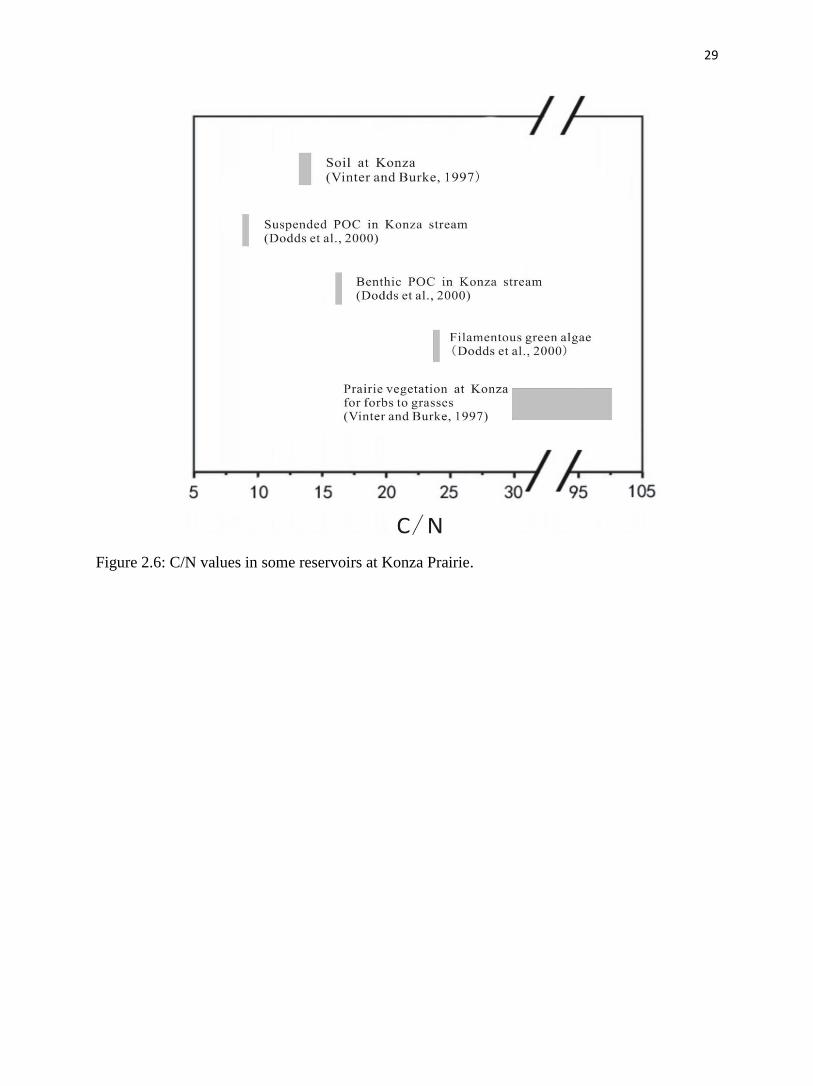
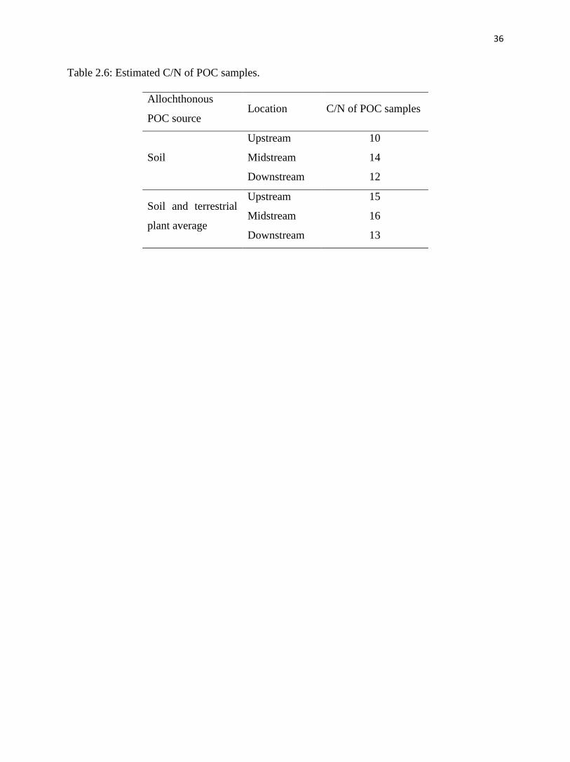
5.5. Implication of estimated C/N of POC samples
Due to low N content of POC samples, it was not possible to calculate the allochthonous
and autochthonous fractions using C/N ratio. Here we use equation (6) to estimate the C/N of
POC samples from C/N of plant samples, soil samples and the allochthonous and autochthonous
fractions obtained from 13
C. The estimated C/N values of POC samples using soil as the
allochthonous source for upstream, midstream and downstream samples are 10, 14 and 12,
respectively (Table 2.6); the estimated C/N values of POC samples derived from soil and
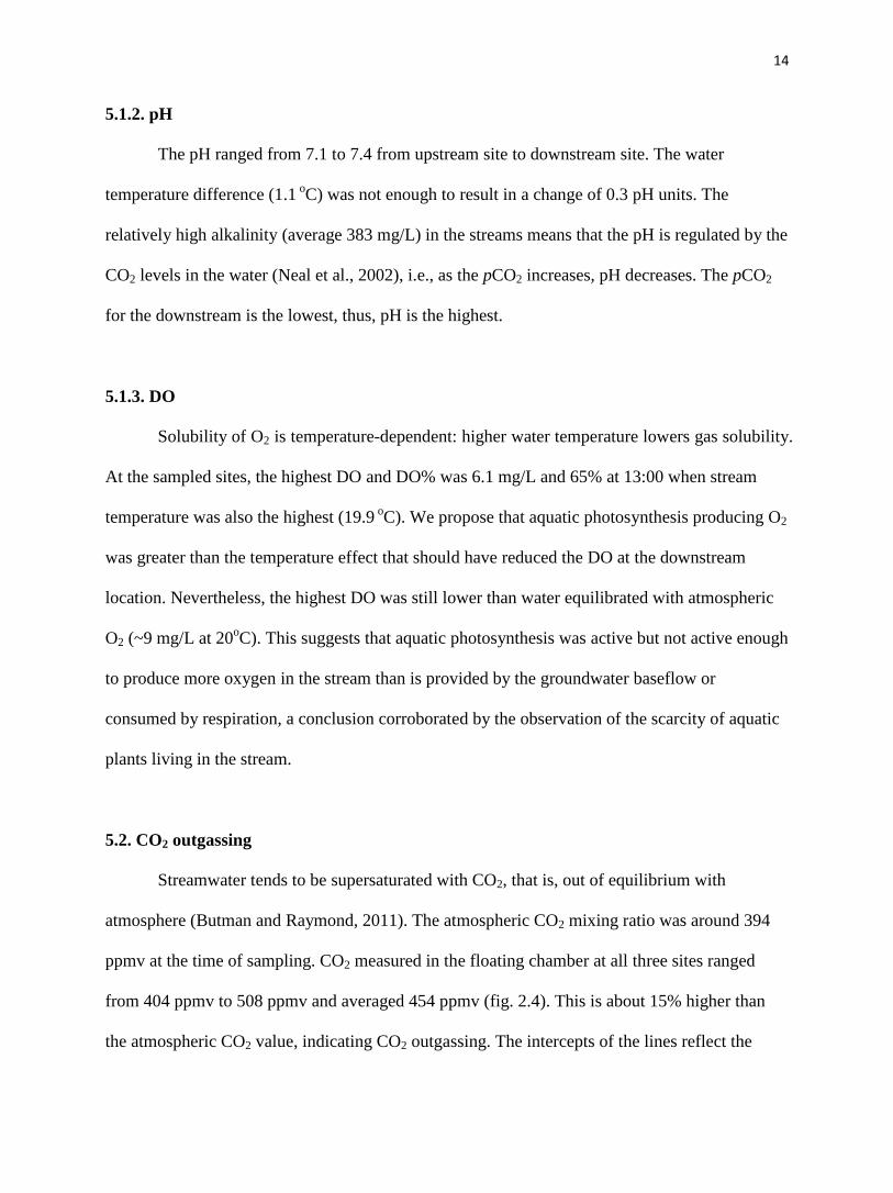
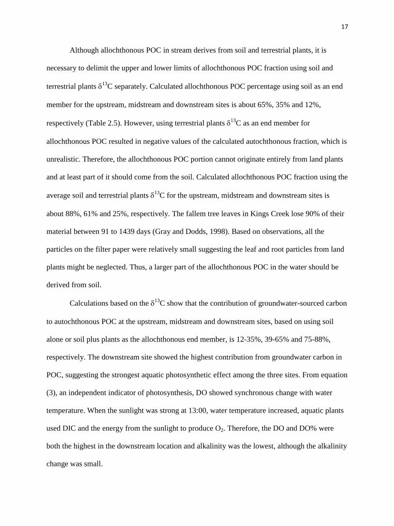
terrestrial plants average (#4 plant excluded) are 15, 16 and 13, respectively. The POC samples
represent suspended POC. According to Dodds et al. (2000), the suspended POC at Konza
Prairie has a C/N value of 9 (fig. 2.6). Our estimation of C/N for POC using soil as the
allochthonous part is close to their measurement, corroborating our finding, above, that soil
should dominate the allochthonous POC.
6. Conclusions
To understand spatiotemporal differences in hydrochemistry in Kings Creek, unstable
parameters (water temperature, pH, DO, SC and Eh) were measured at three locations from
upstream to downstream during midday in May. Soil, plants, water samples and CO2 samples
were taken at those three sites. Thermal images suggest that groundwater temperature was
around 18.3oC and fed the stream from the side and bottom of the stream channel. Results show
that the pH ranged from 7.1 to 7.4. The temperature of the downstream streamwater was the
highest. DO ranged from 4.7mg/L at the upstream site to 6.1mg/L at the downstream site. The
higher DO at the downstream site is attributed to a higher rate of aquatic photosynthesis. CO2
degassing was higher at the downstream site than at the upstream and midstream sites. 13
CDIC
19
was mainly controlled by CO2 outgassing. There was little variation in the other parameters
among the three locations.
The aquatic photosynthesis was the strongest at the downstream site. The autochthonous
POC fraction at the upstream, midstream and downstream sites was about 12-35%, 39-65% and
75-88%, respectively. However, the overall aquatic photosynthesis at Konza was not strong due
to the lack of submerged plants, evidenced by low DO. Estimation of C/N for POC samples at
the three sites is 10-15, 14.0-16 and 12-13. This is comparable to previously measured C/N of
suspended POC and corroborates the conclusion that soil dominates the allochthonous POC in
this portion of Kings Creek.
20
References
Appelo, C.A.J.P., D., 2005. Geochemistry, Groundwater, and Pollution, 2nd
ed. Balkema,
Rotterdam.
Berner, R. A., 2004. The Phanerozoic Carbon Cycle: CO2 and O2: Oxford University Press, 150.
Billings, S. A., R. W. Buddemeier, D. deB. Richter, K. Van Oost, and G. Bohling, 2010. A
simple method for estimating the influence of eroding soil profiles on atmospheric CO2:
Global Biogeochemical Cycles 24, GB2001, doi:10.1029/2009GB003560.
Butman, D., Raymond, P. A., 2011. Significant efflux of carbon dioxide from streams and rivers
in the United States. Nat. Geosci. 4, 839-842.
Cole, J. J., D. L. Bade, D. Bastviken, M. L. Pace, and M. Van de Bogert., 2010. Multiple
approaches to estimating air-water gas exchange in small lakes. Limnol. Oceanogr.
Methods 8, 285–293.
Chiodini, G., Frondini, F., Kerrick, D.M., Rogie, J., Parello, F., Peruzzi, L., Zanzari, A.R., 1999.
Quantification of deep CO2 fluxes from Central Italy. Examples of carbon balance for
regional aquifers and of soil diffuse degassing. Chemical Geology 159, 205-222.
Dodds, W.K., Evans-White, M.A., Gerlanc, N.M., Gray, L., Gudder, D.A., Kemp, M.J., Lopez,
A.L., Stagliano, D., Strauss, E.A., Tank, J.L., Whiles, M.R., Wollheim, W.M., 2000.
Quantification of the nitrogen cycle in a prairie stream. Ecosystems 3, 574–89.
Downing, J. A., J. J. Cole, J. J. Middelburg, R. G. Striegl, C. M. Duarte, P. Kortelainen, Y. T.
Prairie, and K. A. Laube., 2008, Sediment organic carbon burial in agriculturally
eutrophic impoundments over the last century, Global Biogeochem. Cycles, 22, GB1018,
doi:10.1029/2006GB002854.
Dreybrodt, W., 1988. Processes in karst systems, Springer, Heidelberg.
21
Farquhar, G.D., O’Leary, M.H., Berry, J.A., 1982. On the relationship between carbon isotope
discrimination and the intercellular carbon dioxide concentration in leaves. Aust. J. Plant
Physiol. 9, 121–137.
Fritz, P., Fontes, J.C., Frape, S.K., 1989. The isotope geochemistry of carbon in groundwater at
stripa. Geochimica et Cosmochimica Acta 53, 1765–1775.
Gao, Q., Tao, Z., Yao, G., Ding, J., Liu, Z., Liu, K., 2007. Elemental and isotopic signatures of
particulate organic carbon in the Zengjiang River, southern China. Hydrol. Process., 21,
1318–1327.
Gray, L.J., and Dodds, W.K., 1998. Structure and dynamics of aquatic communities. In: Knapp,
A.K., Briggs, J.M., Hartnett, D.C., Collins, S.L. (Eds.), Grassland Dynamics –
Long-Term Ecological Research in Tallgrass Prairie. Oxford University Press, New York,
pp. 177–192.
Hydrologic Benchmark Network Stations in the West-Central U.S. 1963-95, USGS Circular
1173-C
Johnson, W.C., Willey, K.L, Macpherson, G.L., 2007. Carbon isotope variation in modern soils
of the tallgrass prairie: analogues for the interpretation of isotopic records derived from
paleosols. Quat. Int. 162, 3–20
Keller, C.K., Bacon, D.H., 1998. Soil respiration and georespiration distinguished by transport
analyses of vadose CO2, 13
CO2, and 14
CO2. Global Biogeochem. Cycles 12, 361-372.
Kessler, T.J., Harvey, C.F., 2001. The global flux of carbon dioxide into groundwater. Geophys.
Res. Lett. 28, 279-282.
Langmuir D., 1971. The geochemistry of some carbonate ground waters in central Pennsylvania.
Geochim. Cosmochim. Acta, 35, 1023–1045.
22
Liu, Z., Dreybrodt, W., and Wang, H., 2010. A new direction in effective accounting for the
atmospheric CO2 budget: Considering the combined action of carbonate dissolution, the
global water cycle and photosynthetic uptake of DIC by aquatic organisms. Earth-Sci.
Rev., 99, 162–172.
Liu Z, Dreybrodt W, Liu H., 2011. Atmospheric CO2 sink: silicate weathering or carbonate
weathering? Applied Geochemistry, 26, 292-294.
Ludwig, W., Probst, J. L., Kempe, S.,1996. Predicting the oceanic input of organic carbon by
continental erosion. Global Biogeochem. Cy., 10, 23–41.
Macpherson, G. L., Roberts J. A., Blair J. M., Townsend M. A., Fowle D. A., Beisner K. R.,
2008. Increasing shallow groundwater CO2 and limestone weathering, Konza Prairie,
USA. Geochimica et Cosmochimica Acta, v. 72, i. 23, pp. 5581-5599.
Mast, M.A., and Turk, J.T., 1999. Environmental characteristics and water quality of Hydrologic
Benchmark Network stations in the West -Central United States, 1963–95: U.S.
Geological Survey Circular 1173–C, 105 p.
Michaelis, J., Usdowski, E., Menschel, G., 1985. Partitioning of 13
C and 12
C on the degassing of
CO2 and the precipitation of calcite—Rayleigh type fractionation and a kinetic model.
Am. J. Sci. 285, 318-327.
Mook, W.G., Tan, F.C., 1991. Stable carbon isotopes in rivers and estuaries. In: Degens, E.T.,
Kempe, S., Richey, J.E. (Eds.), Biogeochemistry of Major World Rivers. John Wiley,
New York, pp. 345–364.
Neal, C., Watts, C., Williams, R.J., Neal, M., Hill, L., Wickham, H., 2002. Diurnal and longer
term patterns in carbon dioxide and calcite saturation for the River Kennet, south-eastern
England. Sci. Total Environ. 282, pp. 205–231.
23
Parkhurst, D., L., and Appelo, C., A., J., 1999. User’s guide to PHREEQC (Version 2)—a
computer program for speciation, batch-reaction, one-dimensional transport, and inverse
geochemical calculations.U.S. Geol. Surv. Wat.-Resour. Investigations Report 99-4259, p.
312.
Putnam, J.E., Lacock, D.L, Schneider, D.R., Carlson, M.D., and Dague, B.J., 1996. Water
resources data, Kansas, water year 1995: U.S. Geological Survey Water-Data Report KS–
95–1488.
Ransom, M.D., Rice, C.W., Todd, T.C., Wehmueller, W.A., 1998. Soils and soil biota. In: Knapp,
A.K., Briggs, J.M., Hartnett, D.C., Collins, S.L. (Eds.), Grassland Dynamics –
Long-Term Ecological Research in Tallgrass Prairie. Oxford University Press, New York,
pp. 48–66
Sun, H.G., Han, J.T., Zhang, S.R., Lu, X.X., 2011. Transformation of dissolved inorganic carbon
(DIC) into particulate organic carbon (POC) in the lower Xijiang River, SE China: an
isotopic approach. Biogeosciences Discuss. 8, 9471-950.
Tao, F., Liu, C., Li, S., 2009. Source and flux of POC in two subtropical karstic tributaries with
contrasting land use practice in the Yangtze River Basin. Applied Geochemistry, 24,
2102–2112.
Tsypin, M., and Macpherson, G.L., 2012. The effect of precipitation events on inorganic carbon
in soil and shallow groundwater, Konza Prairie LTER Site, NE Kansas, USA. Applied
Geochemistry 27, 2356–2369.
Wood, H. K. and Macpherson, G. L., 2005. Sources of Sr and implications for weathering of
limestone under tallgrass prairie, northeastern Kansas. Applied Geochemistry, 20,
2325-2342.
24
Figure 2.1: Location of Kings Creek and Konza LTER site.
25
Figure 2.2: USGS discharge graph for Kings Creek from March 2012 to September 2012.
26
(a)
(b)
Figure 2.3: Infrared image showing groundwater discharging the stream (a), and visual image of
the same location for comparison (b) (Dr. Andrea Brookfield, KGS).
27
Figure 2.4: Outgassed CO2 concentration vs. time for the upstream, midstream and downstream
in the floating chamber (2-sigma error bars are smaller than the symbols).
350
400
450
500
550
0 50 100 150 200 250
pp
mv C
O2
Sec
Upstream
Midstream, all data
Midstream, datum excluded
Downstream
28
Figure 2.5: 13
C of CO2 vs. time for the upstream, midstream, and downstream in the floating
chamber.
-12.5
-12.0
-11.5
-11.0
-10.5
-10.0
-10.3
-9.8
-9.3
-8.8
-10 40 90 140 190 240
13C
(do
wn
str
ea
m)
13C
(up
str
ea
m a
nd
mid
str
ea
m)
Sec
Upstream
Midstream, all data
Midstream, datum excluded
Downstream
29
Figure 2.6: C/N values in some reservoirs at Konza Prairie.

30
Table 2.1: Data for the Konza stream.
Time Site Field
pH
T
(oC)
SC
(us/cm)
Eh
(mv)
DO
(mg/L) DO%
Alkalinity
(mg/L)
Calculated
CO2 (ppmv)
13
CDIC
(‰)
11:20 Up 7.3 18.8 643 194 4.7 51 384 16800 9.46±0.02
12:10 Mid 7.1 18.9 640 194 4.8 51 385 26800 9.50±0.01
13:00 Down 7.4 19.9 637 198 6.1 65 380 13400 9.19±0.01
31
Table 2.2: 13
C and C/N values for the soil, plant and POC samples
Identifier 13
C VPDB(‰) C/N
Soils
Upstream -20.40 11.0
Midstream -18.56 10.5
Downstream -18.66 10.6
Terrestrial plants
1 (Symphoricarpos
orbiculatus)
-29.50 19.4
2 (Ulmus) -31.08 17.7
3 (C3 unidentified) -30.13 29.8
4 (Elymus villosus) -31.19 82.9
5 (C3 unidentified) -30.39 23.9
6 (Fraxinus
pensylvanica)
-29.12 14.6
7 (C3 unidentified) -30.72 19.3
8 (Bromus inermis) -26.96 22.0
9 (Ouercus macrocarpa) -29.87 18.4
10 (C3 unidentified) -28.55 23.2
Aquatic plants
Upstream (Green alga) -35.90 9.4
Midstream (Polygonum) -32.71 15.9
Downstream (Veronica) -29.96 12.4
POC samples
Upstream -25.86
Midstream -27.70
Downstream -28.58
32
Table 2.3: Measured CO2 concentration in the floating chamber.
Location Time (sec) CO2 ppmv
Upstream
0 404
65 408
125 438
175 457
220 462
Midstream
0 424
60 432
110 440
155 457
195 429
Downstream
0 456
45 485
90 500
130 506
175 508
33
Table 2.4 a: Estimated CO2 flux (F) from CO2 concentration.
Location
F§
(mg/s/m2)
F§
(mg/h/m2)
Daily F§
(mg/d/m2)
Upstream 0.090 330 7800
Midstream 0.062 220 5400
Downstream 0.085 310 7400
§ Flux(mg/s/m2) = 0.001963*(dc/dt)*(V/A)*(273.15/Tm)*(Pm/101.325) (8)
Flux(mg/h/m2) = 7.069*(dc/dt)*(V/A)*(273.15/Tm)*(Pm/101.325) (9)
Flux(mg/d/m2) = 169.6*(dc/dt)*(V/A)*(273.15/Tm)*(Pm/101.325) (10)
dc/dt: increase rate in CO2 partial pressure in the floating chamber; V: chamber volume
(5.73 L); A: chamber bottom area (0.035 m2); 273.15: standard temperature in K; Tm: the
measured temperature of the sampling day in K (22oC+273.15=295.15 K); Pm: the measured
pressure on the sampling day in kPa (barometric pressure from www.wunderground.com for
Manhattan, KS was 29.81 inches Hg, 29.81 * 3.3864 = 100.949 kPa); 101.325: standard pressure
in kPa.
Table 2.4 b: Calculated CO2 flux (F) using k600.
Location
F
(mg/s/m2)
F
(mg/h/m2)
Daily F
(mg/d/m2)
Upstream 0.19 670 16000
Midstream 0.30 1100 26000
Downstream 0.15 530 13000

34
F=k600*(Csur-Ceq) (11)
where k600 (0.50 m/d) is the piston velocity for a CO2 at 20oC, which corresponds to a
Schmidt number of 600. Csur and Ceq (400 ppmv) are surface water and air-equilibrium
concentrations, respectively.
35
Table 2.5: Calculations of autochthonous and allochthonous fractions in POC
Allochthonous
POC source Location
X(autochthonous
fraction, %)
1-X(allochthonous
fraction, %)
Soil
Upstream 35% 65%
Midstream 65% 35%
Downstream 88% 12%
Terrestrial plants
Upstream -63% 163%
Midstream -70% 170%
Downstream -572% 672%
Soil and terrestrial
plant average
Upstream 12% 88%
Midstream 39% 61%
Downstream 75% 25%
36
Table 2.6: Estimated C/N of POC samples.
Allochthonous
POC source Location C/N of POC samples
Soil
Upstream 10
Midstream 14
Downstream 12
Soil and terrestrial
plant average
Upstream 15
Midstream 16
Downstream 13
37
CHAPTER 3. DIEL GEOCHEMICAL VARIATIONS IN A KARST SPRING AND TWO
PONDS, MAOLAN KARST EXPERIMENTAL SITE, CHINA
38
Chapter summary
A karst spring and two downstream ponds fed by the spring at the Maolan Karst
Experimental Site, Guizhou Province, China, were used to investigate the effect of submerged
plants on the CO2 system during a time of spring base flow. Temperature, pH, electrical
conductivity (EC) and dissolved oxygen (DO) were recorded at 15 min intervals for a period of
30 h (12:00 29 August -18:00 30 August, 2012). [Ca2+
], [HCO3-], CO2 partial pressure (pCO2)
and saturation index of calcite (SIC) were estimated from the high-frequency measurements.
Water samples were also collected three times a day (early morning, midday and evening) for
13
CDIC determination. A floating CO2-flux monitoring chamber was used to measure CO2 flux at
the three locations. Results show that there was little or no diel variation in the spring water
parameters. In the midstream pond with flourishing submerged plants, however, all parameters
show distinct diel changes: temperature, pH, DO, SIc, 13
CDIC increased during the day and
decreased at night, while EC, [HCO3-], [Ca
2+], and pCO2 behaved in the opposite sense. In
addition, maximum DO values (16~23 mg/L) in the midstream pond at daytime were two to
three times those of water equilibrated with atmospheric O2, indicating strong aquatic
photosynthesis. The proposed photosynthesis is corroborated by the low calculated pCO2 of
20-200 ppmv, which is much less than atmospheric pCO2. In the downstream pond with fewer
submerged plants but larger volume, all parameters displayed similar trends to the midstream
pond but with much less change, a pattern that we attribute to the lower biomass/water volume
ratio. The diel hydrobiogeochemical variations in the two ponds depended essentially on
illumination, indicating that photosynthesis and respiration by the submerged plants are the
dominant controlling processes. The large loss of DIC between the spring and midstream pond,
attributed to biological effects, demonstrates that natural surface water systems may constitute an
important sink of carbon (on the order of a few hundred tons of C km2/a) as DIC is transformed

39
to autochthonous organic matter. The rates of sedimentary deposition and preservation of this
organic matter in the ponds, however, require quantification in future work to fully assess the
karst processes-related carbon cycle, especially under global climate and land use changes.
40
1. Introduction
Hydrobiogeochemical behavior in karst terrains exhibits marked annual, seasonal, and
even diurnal and storm-scale variations (Liu et al., 2004; Liu et al., 2006; Liu et al., 2007; Liu et
al., 2008). Thus, an increasing number of studies have focused on the karst critical zone because
of its sensitivity to environmental changes and distinctive resource-environmental effects (De
Montety et al., 2011; Hayashi et al., 2012; Yang et al., 2012; Zeng et al., 2012).
Surface waters in karst terrains are rich in dissolved inorganic carbon (DIC) and provide
a well-defined natural system to study gas exchange between water and atmosphere, calcite
deposition, aquatic photosynthesis and respiration (Spiro and Pentecost, 1991). Previous studies
have emphasized particular aspects of geochemistry or biology in these waters, but data on the
interactions among physical, chemical and biological processes are still lacking. These mutually
dependent processes should be discussed together, because consideration of
water-rock-gas-organism interaction as a whole is required to understand the spatiotemporal
hydrobiogeochemical variations in karst waters (Liu et al., 2010; Yang et al., 2012). Moreover,
due to the dynamics and complexity of karst processes, there is still much to be learned about the
geochemistry of karst waters, especially diel spatiotemporal variation (Liu et al., 2007; Liu et al.,
2008; Yang et al., 2012).
A study of dissolved elemental and carbon isotopic composition in the major karst
springs at the Maolan Karst Experimental Site, SW China (Maolan) has provided useful
information about the characteristics of spring water. Because different sources of dissolved
inorganic carbon (DIC) have different isotopic compositions, 13
CDIC is a direct reflection of the
physical, chemical and biological processes in the water (Han et al., 2010). Identifying the
transformation of DIC to organic carbon (OC) as evidenced by changes in CO2, O2, DIC,
pH,13
CDIC and estimating this contribution are the purposes of this study.
41
Here we report on an investigation of an epikarst spring (Liu et al., 2007) and its two
downstream ponds at Maolan. We have obtained high time-resolution monitoring records of the
physical-chemical parameters for about a 30-hour period (12:00 29 August -18:00 30 August,
2012). We also report selected 13
CDIC from the site. This research focuses on the physical
chemistry of karst water and the evolution of 13
CDIC influenced by major natural processes. The
aim of this study is to understand diurnal hydrobiogeochemical variations in a typical karst
spring and its two downstream ponds under summer, sunny and base flow conditions. These
conditions represent the time of most intensive biological activity. The results reveal
spatiotemporal differences and their underlying mechanisms, which have implications for
assessing karst processes as related to the global carbon cycle (Liu et al., 2010).
2. Study area
The Maolan Karst Experimental Site in China (Maolan; fig. 3.1) is well known for its
dense virgin evergreen forests growing on cone karst, and is listed by UNESCO as a world
heritage site (Libo Karst, one of the three clusters of South China Karst, whc.unesco.org).
Annual rainfall in areas with virgin forest is about 1750 mm, about 80% of which falls in the
monsoon season from April to September, July and August being the months with highest
average precipitation (Zhou, 1987). Annual rainfall is 400 mm less in surrounding deforested
areas due to absence of the forest microclimatic effect (Zhou, 1987). The mean annual air
temperature at Maolan is about 17°C, with hot summers (June–August) and cold winters
(December–February). The bedrock is mostly dolomitic limestone of Middle to Lower
Carboniferous age (Liu et al., 2007; Jiang et al., 2008).
The sampled spring is a typical Ca-HCO3 type epikarst spring (here termed ‘Maolan
spring’) with flow rate of 0.05–30 L/s (Liu et al., 2007). It is at the base of a cone karst slope
42
covered by virgin karst forest. There is no net deposition of tufa at the spring and the calcite
saturation index of the water there is near zero (Liu et al., 2007). Fig. 3.2 gives an oblique
perspective of the spring and the receiving ponds with different amounts of submerged plants
(chiefly Charophyta). The spring and two ponds have been modified by the addition of weirs to
control outflow. The spring weir was built in 2002 for long-term monitoring of water stage and
hydrogeochemistry (Liu et al., 2007), and the weirs for the two ponds were built in 2004 by the
local population for freshwater fish farming; fishing was abandoned in 2011.
The spring discharge was 1.2 L/s and almost stable during the study period, and the
surface areas of midstream and downstream ponds were 280 m2 and 1300 m
2 respectively. The
midstream pond volume was smaller (60 m3) than the downstream pond volume (1300 m
3). The
distances from the spring orifice sampling site to the midstream pond sampling site was 38 m,
and the distance between the midstream and downstream pond sampling sites was 29 m.
3. Methods
3.1. Field monitoring and sampling
The field study was conducted on 29-30 August 2012 under sunny weather during the
wet season. Two WTW® (Wissenschaftlich-Technische-Werkstaetten) Technology MultiLine®
350i’s and one SEBA® multi-parameter data logger (Qualilog-16®) were programmed to collect
continuous readings of pH, water temperature, dissolved oxygen (DO), and electrical
conductivity (EC, 25oC) at 15 min interval for 30 hours (12:00 29 August-18:00 30 August,
2012). The meters were calibrated prior to deployment using pH (4, 7 and 10), EC (1412 s/cm),
and DO (0% and 100%) standards. One WTW-350i® was located at the spring orifice to
characterize discharging groundwater. The Qualilog-16® monitored conditions at the midstream
43
pond and the second WTW-350i® monitored the downstream pond. The resolutions on pH, DO,
EC and temp. are 0.01, 0.01 mg/L, 1 s /cm and 0.01oC, respectively.
Water samples for 13
CDIC were collected three times (midday 29 August; evening 29
August; morning 30 August) at the three sites. The sampling site for the Maolan spring 13
CDIC
differed from the location of the multi-parameter meter: the meter was put in the orifice
measuring groundwater conditions just before emergence into the spring pool, whereas the
13
CDIC samples were collected in the spring pool, after some equilibration with surface
conditions. The 13
CDIC samples were collected in pre-cleaned 30 mL glass vials, with no air
space. One drop of saturated HgCl2 solution in each sample served to prevent microbial activity
and all samples were kept at temperatures below 4oC until analysis.
A floating CO2-flux monitoring chamber (14 L volume with diameter of 40 cm, and
surface area of 0.126 m2) was placed on the surface of the waters to determine CO2 efflux from
the three sites. CO2 flux was evaluated three times (midday 29 August; evening 29 August;
morning 30 August) at each location by collecting five floating-chamber gas samples at 2-min
intervals. The CO2 concentration of the samples was measured by gas chromatography
(Agilent-7890®) with a resolution of 0.01 ppmv.
3.2. Estimating CO2 partial pressure and the calcite saturation index
We attribute EC fluctuations in the spring and ponds to Ca2+
and HCO3- variations
induced by calcite precipitation or dissolution because other dissolved components are not
involved in dissolution or precipitation reactions, no rainfall occurred during the sampling
interval and evaporation is unlikely because of the high humidity (83% annually,
www.163gz.com) of Maolan. Ca2+
, Mg+2
and HCO3- were previously correlated with EC at this
44
site (Liu et al., 2007). The regressions were used to estimate concentrations of Ca2+
and HCO3-
for further calculations, below. The relationships are:
[Ca2+
] = 0.15 EC - 0.78, r2
= 0.94, (1)
[Mg2+
] = 0.04 EC + 0.22, r2
= 0.77, (2)
[HCO3-] = 0.63 EC - 4.70, r
2 = 0.99, (3)
where brackets denote concentrations in mg/L and EC is electric conductivity in S/cm at 25oC
(Liu et al., 2007).
Water temperature, pH, estimated Ca2+
and HCO3-, with mean monthly values of K
+,
Na+, Mg
2+, Cl
– and SO4
2– (resolutions are 0.01 mg/L) (Liu et al., 2007), were speciated using
PHREEQC (Parkhurst and Appelo, 1999) to calculate CO2 partial pressure (pCO2) and the
calcite saturation index (SIc) for each record.
3.3. Determining DIC and 13
CDIC
The pH of the water in the study ranged from 7.20 to 9.63. At pH 9.6, HCO3- and CO3
2-
are 84% and 16% of the DIC, respectively. At pH 9, HCO3- and CO3
2- constitute 96% and 4% of
the DIC, respectively. However, only four pH points for the midstream pond have values higher
than 9.5. Thus, calculated HCO3- is used as an approximation of DIC for this study.
13
C was analyzed on a MAT-252 mass spectrometer with dual inlet. The results are
reported relative to the V-PDB standard with an uncertainty less than +/- 0.03‰ (Sun et al.,
2011).
45
4. Results
4.1. Diel variations in physical chemistry and 13
CDIC
Fig. 3.3 shows the diel variations of the physical chemistry of the Maolan spring and
ponds during the study of 29-30 August 2012. Each location is discussed separately, below.
4.1.1. Maolan spring
The pH values of the spring water ranged from 7.11 to 7.28, averaging 7.21. Except for
fluctuations of DO (coefficient of variation, CV=4%) and pCO2 (CV=6%; Table 3.1), there was
almost no diel change in all of the other physical and chemical parameters at the spring
(CV<1.0%, Table 3.1, fig. 3.3). 13
CDIC of Maolan spring was lowest in the sample collected in
the morning and highest at midday (fig. 3.4).
4.1.2. Midstream pond
All parameters in the midstream pond showed distinct changes over the sampling period
(fig. 3.3, Table 3.1). Temperature, pH, DO, SIc and 13
CDIC increased during the day and
decreased at night, while EC, HCO3-, Ca
2+, and pCO2 decreased in the daytime and increased at
the night (figs. 3.3 and 3.4).
Water temperature in the midstream pond ranged from 24.2oC at 8:00 and 31.8
oC at
16:00 in response to insolation; the mean value was 27.7oC (fig. 3.3, Table 3.1).
Correspondingly, pH, DO, SIc and 13
CDIC of the waters increased during the day and peaked at
9.62, 23.49 mg/L, 1.62, and -8.4‰, respectively, about an hour or two after temperature was the
highest. These parameters gradually declined during the night to reach lowest values (7.47, 0.05
mg/L, 0.03, and -12.3‰, respectively) in the early morning before the sun rose. EC, HCO3-, Ca
2+
and pCO2 displayed the reverse of this behavior; EC, estimated HCO3-, estimated Ca
2+ and pCO2
46
continuously decreasing during the day to a minima (249 s/cm, 152 mg/L, 37 mg/L, and 20
ppmv, respectively) around 18:00, then gradually increased to a maxima (335 s/cm, 206 mg/L,
50 mg/L, and 6750 ppmv, respectively) in the early morning.
4.1.3. Downstream pond
All of the parameters in the downstream pond followed patterns similar to those in the
midstream pond from morning to midday but at lower amplitude (fig. 3.3, Table 3.1). Water
temperature varied from 26.7oC
to 30.5
oC with an average of 28.6
oC, reaching its minimum at
about 8:00 and peak at around 16:00. Similarly, EC, estimated HCO3-, estimated Ca
2+ and pCO2
decreased from 301 S/cm, 185 mg/L, 44 mg/L and 1430 ppmv respectively at 8:00 to 280
S/cm, 172 mg/L, 41 mg/L and 660 ppmv at around an hour or two after temperature peaked
(fig. 3.3, Table 3.1). pH, DO, and SIc of the water increased from 8.12, 6.95 mg/L, and 0.66
respectively at 8:00 to 8.43, 11.5 mg/L, and 0.93 at about one or two hours after maximum
temperature.
4.2. CO2 flux
4.2.1. Maolan spring
Fig. 5a, Table 3.2 and Table 3.3 show that CO2 degassing in the spring pool was the
weakest during midday and the most intense in the evening. In the morning, CO2 increased from
504 ppmv to 602 ppmv after 8 minutes, with an efflux of 2500 mg/d/m2. During midday, initial
CO2 concentration was 382 ppmv and gradually increased to 416 ppmv after 8 minutes, with an
efflux of 1400 mg/d/m2. In the evening, the starting CO2 concentration in the chamber was 566
ppmv and increased to 660 ppmv over the measurement period of 8 minutes, with an efflux of
3100 mg/d/m2.
47
4.2.2. Midstream pond
CO2 concentration ranged from 517 ppmv to 544 ppmv after 6 minutes and 491 ppmv to
518 ppmv after 8 minutes in the morning and evening samplings, respectively, (fig. 3.5b), with
both effluxes of 1100 mg/d/m2 (Table 3.3). During midday, there was no CO2 outgassing.
Instead, atmospheric CO2 evidently dissolved into the pond water. CO2 started at 364 ppmv in
the chamber then gradually decreased to 273 ppmv after 8 minutes, with an influx of -3600
mg/d/m2.
4.2.3. Downstream pond
CO2 concentration was the highest in the morning, varying from 534 ppmv to 551 ppmv
in the chamber within 8 minutes, with an efflux of 500 mg/d/m2. In the midday and evening, it
increased from 385 to 433 ppmv after 8 minutes and 446 to 470 ppmv after 8 minutes
respectively, with effluxes of 960 mg/d/m2 and 560 mg/d/m
2, correspondingly (fig. 3.5c, Table
3.3).
5. Discussion
5.1. Mechanisms for DIC and 13
CDIC changes in the Maolan spring pool
Atmospheric CO2 has an isotopic composition of 13
C of -7‰, and the isotopic
composition of marine limestone is 0 +/-5‰ (Telmer and Veizer, 1999). Generally speaking, the
13
C of CO2 derived from respiration of C3 plant roots is similar to the 13
CCO2 from degradation
of soil organic matter derived from C3 plants, which is close to -24 ± 2‰ (Cerling et al., 1991;
Aucour et al., 1999). According to a recent study in the Maolan spring catchment, 13
CDIC ranges
from -8.1‰ to -16.6‰ with a mean value of -13.4‰ (Han et al., 2010), which encompasses the
range in this study of -13.4‰ to -14.3‰, with a mean value of -13.9‰ (fig. 3.4). These 13
C
48
values are lower than those of karst groundwater measured in city springs in southwest China
(Han et al., 2010), the difference attributed to the dense virgin forests in Maolan. Han et al.
(2010) also showed that 56 ± 9% of the DIC in the Maolan spring water is from degradation of
organic matter in the soil and the remainder from dissolution of carbonate.
In this study, the 13
CDIC of the Maolan spring pool started at -13.4‰ at 13:30 on 29
August then decreased to -14.0‰ at 19:40, and continued decreasing to -14.3‰ at 7:30 of 30
August. It is unlikely that the diel variation of the 13
CDIC in the spring pool was caused by the
dissolution of calcite or the degradation of soil organic matter for the following reasons. First,
the degradation of soil organic matter would be the most intense during midday when the air
temperature was the highest, resulting in more CO2 entering the groundwater. This would affect
the 13
CDIC in two ways. On the one hand, lighter CO2 from soil organic matter degradation
would cause depletion of the 13
CDIC. On the other hand, higher CO2 could drive calcite
dissolution and increase the 13
CDIC because of the heavier 13
C of limestone. Because the
13
CDIC at 13:30 was the highest, organic matter degradation is not likely the main influence on
the 13
CDIC. Second, the SIc, [Ca2+
] and [HCO3-] of the spring were stable and SIc was always
slightly below 0 (fig. 3.3), indicating the groundwater was undersaturated with respect to calcite.
This suggests that there was little precipitation/dissolution of limestone in the spring. Because
the diel variation of the 13
CDIC in the spring pool is not likely controlled by organic matter
degradation or calcite dissolution, it is most likely controlled by the change in CO2 efflux or
aquatic photosynthetic uptake of CO2.
CO2 outgassing (efflux) causes an enrichment of δ13
CDIC in the residual DIC. One study
documented shifts in δ13
CDIC of up to 5‰ as a result of CO2 outgassing at carbonate springs
(Michaelis et al., 1985). According to Fig. 3.5a and Table 3.3, CO2 efflux was the weakest at the
midday sampling and most intense in the evening. If CO2 efflux was the primary influence on
49
δ13
CDIC, then δ13
CDIC should be the lightest at midday and the heaviest in the evening, the
opposite of what is observed. Therefore, the observed δ13
CDIC pattern is most likely related to the
change in aquatic photosynthetic uptake of CO2 by the submerged plants in the spring pool (fig.
3.6), stronger during midday when insolation is high than in the early morning and evening. It
should be pointed out that the reason why all the physical and chemical parameters of the spring
did not fluctuate was because the WTW350i electrode was placed in the spring orifice, free from
any photosynthesis activity and thus reflecting the characteristics of groundwater without any
modification from the open surface. However, the water samples for the 13
CDIC determination
and degassed CO2 samples were collected in the spring pool where they were already affected by
aquatic photosynthesis (fig. 3.7). Because photosynthesis utilizing CO2 was most intense at
noontime and in the evening, CO2 outgassing was the weakest at this time, consistent with our
data from the floating chamber.
5.2. Mechanisms for diel variations in physical, chemical and isotopic properties of the
midstream pond
Physical and chemical parameters of surface water may be controlled by groundwater
input, temperature changes, gas exchange between water and atmosphere, aquatic photosynthesis
and respiration, and calcite precipitation and dissolution (Spiro and Pentecost, 1991). These are
discussed below.
5.2.1. Groundwater input
From the data in Fig. 3.3, little or no diurnal variations were observed in the
physical-chemical parameters of the Maolan spring: groundwater parameters were stable and
50
thus the diel changes in physical and chemical properties in the midstream pond were not caused
by changes in the groundwater input.
5.2.2. Temperature
Solubility of both O2 and CO2 are temperature-dependent with higher solubility when
water temperature is low. In the midstream pond, pH and DO increased and pCO2 decreased
when water temperature increased during the day, and all trends reversed as temperature
decreased at night (fig. 3.7a, 3.7b). Although the pH and pCO2 trends follow the expected trends
for temperature control on gas solubility, the DO trend is the opposite of what is expected. This
suggests that changes in water temperature might not be the major factor controlling pH, pCO2,
and DO in the midstream pond during the study period.
5.2.3. Gas exchange between water and atmosphere
Inland streams and rivers tend to be CO2-supersaturated with respect to the atmosphere
and thus, are a net source of CO2 to the atmosphere (Butman and Raymond, 2011). Gas exchange
between water and air can induce large diurnal variations in DO and pCO2, the major controls of
Eh and pH (Hoffer-French and Herman, 1989; Liu et al., 2006; Liu et al., 2008). In this study,
pCO2 and DO followed opposite trends in the midstream pond (fig. 3.7c).
CO2 outgassing should be the weakest at midday and highest in the morning in the
midstream pond, as inferred from the estimated pCO2 values and measured CO2 concentrations
in the floating chamber (fig. 3.5, Table 3.2). CO2 degassing enriches 13
CDIC in streams (Doctor
et al., 2008). The expected highest rate of outgassing in the early morning should have yielded
the highest 13
CDIC. Instead, the highest 13
CDIC was at midday, when the estimated pCO2 was
the lowest.
51
These observations and trends indicate that outgassing may not have been the dominant
factor controlling pH, concentrations of DO and CO2, and 13
CDIC during the study period.
5.2.4. Photosynthesis and respiration by submerged plants
Diurnal variations of DO and pCO2 are commonly influenced by aquatic photosynthesis
and respiration processes which can be approximated by standard equations (e.g., Liu et al.,
2008):
6H2O + 6CO2 C6H12O6 +6O2 Photosynthesis (4)
C6H12O6 +6O2 6H2O + 6CO2
Respiration
(5)
Measured DO showed synchronous variation with water temperature, and inverse correlation
with pCO2 (fig. 3.7), suggesting a link to photosynthesis and respiration. During the day when
the rate of photosynthesis exceeded respiration, submerged plants used DIC and the energy from
the sunlight to produce organic matter and O2. Fig. 3 shows that when sunlight was strong during
the day, water temperature increased until 16:00 and DO increased until 18:00. pH of the water
increased as photosynthesis consumed CO2. On the other hand, respiration occurs at all times,
consuming O2 and releasing CO2.. Therefore, after 16:00 when water temperature started to
decrease, DO and pH decreased by the respiration release of CO2 into the water, with a time lag
of one or two hours. During the night, in the absence of photosynthesis, respiration was
dominant, and consequently DO and pH fell to their minima and pCO2 peaked (fig. 3.3). The
inverse relationship between pCO2 and DO over the study period (fig. 3.7c) suggests that the
effect of aquatic biological processes surpassed the temperature effect and outgassing. We
suggest biological processes are the main factors dominating pH, concentrations of DO and CO2,
and 13
CDIC in the midstream pond on a daily timescale under climatic conditions similar to those
during the study period.
52
5.2.5. Calcite precipitation/ dissolution
The decrease in Ca2+
concentration between Maolan spring and the midstream pond (fig.
3.3, Table 3.1) suggests that calcite was being precipitated in the midstream pond. During the
daytime, submerged plants utilize CO2 and therefore DIC in the ponds, thereby increasing the
pH, and potentially driving calcite precipitation. During the nighttime, with the absence of
photosynthesis, submerged plants release CO2 back into the water by respiration, thereby
increasing the solubility of calcite, and potentially driving calcite dissolution in the midstream
pond. The following equations can express these processes (Liu et al., 2010):
Ca2+
+ 2HCO3– CaCO3 + X(CO2 +H2O)+(1-X)(CH2O+O2) (daytime) (6)
CaCO3 + CO2 +H2O Ca2+
+ 2HCO3–
(nighttime)
(7)
where X and 1-X are stoichiometric numbers.
When calcite precipitates (which enriches 13
C, with ~2‰ heavier than HCO3-, Deines et
al., 1974) and organic matter forms (which enriches 12
C, with ~15‰ lighter than HCO3-, Sun et
al., 2011) during the day, EC, Ca2+
and HCO3- concentrations all decrease, causing depletion of
12C in the remaining DIC in water (i.e., increase in
13CDIC). At night, the EC, Ca
2+, HCO3
-
concentrations increase due to calcite dissolution and 13
CDIC decreases due to release of light
12CO2 into water from respiration. However, EC, Ca
2+ and HCO3
- in the midstream pond never
exceeded those in Maolan spring (fig. 3.3). Moreover, SIc of the midstream water ranged from
0.03~1.62 which is always at least slightly oversaturated with respect to calcite, indicating no
carbonate dissolution. Therefore, carbonate dissolution in the midstream pond is an unlikely
mechanism contributing to variations in 13
CDIC on a daily timescale.
53
5.3. Mechanisms for diel variations in physical, chemical and isotopic properties of the
downstream pond
An analysis of the same factors addressed in the midstream pond also applies to the
downstream pond. When the sun rose at 8:00, the water temperature started to increase and DO
increased rather than decreased. Thus, the DO increase likely resulted from aquatic
photosynthesis. pCO2 decreased causing higher pH. The variations of the chemical parameters in
the downstream pond were much less than those in the midstream pond, as were variations in
13
CDIC values. In the downstream pond, however, the 13
CDIC value lower at midday than in the
evening may be explained by the deposition of more calcite at midday, which enriches in 13
C,
leaving DIC rich in 12
C (Deines et al., 1974; Michaelis et al., 1985).
The reduced amplitude of the variations in the downstream pond in comparison with the
midstream pond may result from the larger volume in the downstream pond that buffered the
system. The depth of the downstream pond water was around 1 m, while the depth of the
midstream pond water was less than 0.2 m. With the surface areas of about 1310 m2
and 284 m2,
water volumes were estimated to be about 1300 m3 and 60 m
3 in the downstream and midstream
ponds, respectively. The volume effect was further intensified by the lower biomass (submerged
plants) in the downstream pond than in the midstream pond, as indicated by the water color
(fig.3.2).
5.4. Contribution of aquatic biological effects to the stability and sink of carbon
5.4.1. Transformation of DIC into OC: organic carbon preservation potential
The initial DIC of the midstream pond water was contributed mainly by the Maolan
spring and the initial DIC of the downstream pond water was controlled by the midstream pond
water input. DIC concentration in the midstream and downstream ponds waters were always
54
lower than that of the spring water. The average estimated DIC concentration of the spring was
224 mg/L, while the average estimated DIC concentrations of the midstream and downstream
ponds were 187 mg/L and 182 mg/L, respectively. The decrease in the DIC concentrations
between the spring and the midstream pond, and between the midstream pond and the
downstream pond reflects the loss of inorganic carbon. The processes influencing the DIC
concentrations in the two ponds were: (1) precipitation and dissolution of calcite, (2) exchanges
with atmospheric CO2, and (3) aquatic photosynthetic and respiratory.
Since this loss of DIC will be partly transformed into TOC (Sun et al., 2011) as stated in
equation (6), and eventually partly buried as autochthonous organic matter (OC) (Liu et al.,
2011, Fig. 3.8), it constitutes a “biological carbon pump” (De La Rocha and Passow, 2007) and
increases the organic carbon preservation potential in the ponds. Moreover, if the terrestrial
“biological carbon pump” effect is strong enough, as in the case of midstream pond, there is even
a CO2 sink directly from the atmosphere to surface waters (fig. 3.5b, Table 3.3) as discussed
below in more detail.
5.4.2. CO2 influx from atmosphere to water: insight from the floating chamber data in the
midstream pond
During 13:00-19:00, the strong aquatic photosynthesis (with high DO concentrations)
resulted in pCO2 levels of less than 100 ppmv (Fig. 3.3, Table 3.1). Further, CO2 concentration in
the chamber started with 364 ppmv at 14:51 then gradually decreased to 273 ppmv after 8
minutes (fig. 3.5b). The pCO2 in the chamber was lower than that of the atmosphere (around 390
ppmv), suggesting that there was CO2 influx from the atmosphere to water instead of CO2
evasion. This phenomenon in the midstream pond suggests that strong aquatic photosynthesis in
terrestrial surface waters might form another important natural carbon sink by drawing CO2
55
directly from the atmosphere, as occurs in the oceans (Ducklow et al., 2001; Passow and
Carlson, 2012).
5.4.3. Quantification of daily organic carbon formation in the two ponds
The decrease in DIC between Maolan spring and the ponds results from the joint effects
of calcite precipitation, exchanges with atmospheric CO2, and aquatic photosynthesis. We have
used the decrease in Ca2+
concentrations to predict calcite precipitation (Table 3.1) and the flux
of exchanges with atmospheric CO2 (Table 3.3) in the two ponds. The daily organic carbon
formation in the two ponds can be estimated as follows:
MOC=Q *(DIC1-DIC2)/5.080– Q *(Ca1-Ca2)/3.337 – (F/3.664)*A
where MOC is mass of organic carbon formed in a day (mg/d); Q is the discharge of the stream
(i.e., the discharge of the spring if evaporation is ignored under conditions of high humidity, L/d),
DIC1 and DIC2 are the HCO3- concentrations at the inlet and outlet of the pond (in mg/L), 5.080
is the HCO3-—carbon conversion factor, Ca1 and Ca2 are the Ca
2+ concentrations in mg/L at the
inlet and outlet of the pond, respectively, 3.337 is the calcium-carbon conversion factor,
(40.08/12.011), F is the CO2 flux from water surface (mg/d/m2), 3.664 is the CO2-carbon
conversion factor, and A is the area of pond water surface (m2).
For the midstream pond:
MOC=103680*(223.6-186.6)/5.080-103680*(53.5-44.8)/3.337-(-450/3.664)*280
=519000 (mg/d);
For the downstream pond:
MOC=103680*(186.6-182)/5.080-103680*(44.8-43.7)/3.337-(670/3.664)*1300
= -178000 (mg/d).
56
Therefore, the organic carbon sink flux by the submerged plants in the midstream pond is ~1850
mg/d/m2, equivalent to 677 t C/km
2/a, which shows the significant role of submerged plants in
stabilizing the carbon sink by karst processes (carbonate weathering) (from DIC to TOC) and/or
uptake of CO2 directly from the atmosphere.
The organic carbon sink flux in the downstream pond is -137 mg/d/m2, equivalent to
-49.9 t C/km2/a, the negative value showing no net organic carbon sink by the few submerged
plants in the downstream pond, but, instead, release of CO2 by decomposition of allochthonous
organic matter. We assume this organic matter is the legacy of fish farming, ceased ~ 1 year
before this study, in the downstream pond.
6. Conclusions
Physical and chemical parameters (water temperature, pH, DO, and EC) were monitored
at high time-resolution (15 min) over a 30-hour period to investigate the controls on
hydrobiogeochemistry at the Maolan Karst Experimental Site, Guizhou province, China. The
study site included a karst spring and two downstream ponds with different development of
submerged plants, and sampling occurred under wet-season, summer, sunny, base-flow
conditions. [Ca2+
], [HCO3-], CO2 partial pressure (pCO2) and saturation index of calcite (SIc)
were estimated from the high-resolution measurements. Samples for 13
CDIC were collected three
times over the 30-hour period (midday, early evening and early morning) at the three locations.
Gas samples collected from a floating chamber were used to calculate CO2 efflux from the three
locations.
Results show that there was little or no diel variation in most of the spring physical and
chemical parameters. The midstream pond, assumed to have received input only from the spring
~38 meters upgradient, was filled with submerged plants, and all physical and chemical
57
parameters showed distinct diel changes. The temperature, pH, DO, SIc, 13
CDIC in the
midstream pond increased during the day and decreased at night, while EC, HCO3-, Ca
2+, and
pCO2 decreased during the day and increased at the night. The maximum DO values (16~23
mg/L) in the midstream pond during the day were twice to three times those expected of water
equilibrated with atmospheric O2, suggesting aquatic photosynthesis. The midstream pond had
the lowest estimated pCO2 of the three locations, at 20 ppmv, which is much less than the
atmospheric CO2 concentration, also suggesting aquatic photosynthesis. In addition, during the
midday sampling time, the CO2 flux direction was from the atmosphere into water. The
downstream pond had only a few submerged plants. At this location, all of the parameters varied
similarly to the midstream pond location, but with much lower amplitude. We suggest this results
from the dilution effect because of the lower biomass/water tank ratio. The diel
hydrobiogeochemical temporal variations in the two ponds are consistent with results expected
from aquatic photosynthesis and respiration.
The large loss of DIC between spring and midstream pond is attributed to biological
storage of carbon, demonstrating that natural surface waters may constitute an important carbon
sink. Since this loss of DIC is at least partly and likely mostly transformed into TOC, burial as
autochthonous organic matter constitutes a “terrestrial biogeochemical carbon pump” (TBCP).
Moreover, if the TBCP effect is strong enough, as in the case of midstream pond under optimum
photosynthesis conditions, there is a CO2 sink directly from the atmosphere to surface waters.
The distribution and extent of surface waters with strong TBCP is as yet unknown. In
addition, sedimentation and preservation rates of autochthonous OC (fig.3.8) in terrestrial surface
water is also poorly known, especially under rapid global climate and land use changes occurring
recently. This study suggests that an important goal in improving global carbon budgets may
include quantifying the importance of the TBCP in terrestrial aquatic settings.
58
References
Aucour, A. M., Sheppard, S. M. F., Guyomar, O., Wattelet, J., 1999. Use of 13
C to trace origin
and cycling of inorganic carbon in the Rhone river system. Chem. Geol. 159, 87–105.
Butman, D., Raymond, P. A., 2011. Significant efflux of carbon dioxide from streams and rivers
in the United States. Nat. Geosci. 4, 839-842.
Cerling, T. E., Solomon, D. K., Quade, J., 1991. On the isotopic composition of carbon in soil
carbon dioxide. Geochim Cosmochim Acta 55, 3403–3405.
De La Rocha, C. L., Passow, U., 2007. Factors influencing the sinking of POC and the efficiency
of the biological carbon pump. Deep Sea Res. 54, 639–658.
De Montety, V., Martin, J.B., Cohen, M.J., Foster, C., Kurz, M.J., 2011. Influence of diel
biogeochemical cycles on carbonate equilibrium in a karst river. Chem. Geol. 283, 31-43.
Deines, P., Langmuir, D., Harmon, R. S., 1974. Stable carbon isotope ratios and the existence of
a gas phase in the evolution of carbonate ground waters. Geochim. Cosmochim. Acta. 38,
1147-1164.
Doctor, D. H., Kendall, C., Sebestyen, S. D., Shanley, J.B., Ohte, N., Boyer, E.W., 2008. Carbon
isotope fractionation of dissolved inorganic carbon (DIC) due to outgassing of carbon
dioxide from a headwater stream. Hydrol. Process. 22, 2410-2423.
Ducklow, H. W., Steinberg, D. K., Buesseler, K. O., 2001. Upper ocean carbon export and the
biological pump. Oceanography 14, 50-58.
Han, G., Tang, Y., Wu, Q., 2010. Hydrogeochemistry and dissolved inorganic carbon isotopic
composition on karst groundwater in Maolan, southwest China. Environ. Earth Sci. 60,
893-899.
59
Hayashi, M., Vogt, T., Machler, L., Schirmer, M., 2012. Diurnal fluctuations of electrical
conductivity in a pre-alpine river: Effects of photosynthesis and groundwater exchange. J.
Hydrol. 450, 93-104.
Hoffer-French, K., Herman, J., 1989. Evaluation of hydrological and biological influences on
CO2 fluxes from a karst stream. J. Hydrol. 108, 189-212.
Jiang, G., Guo, F., Wu, J., Li, H., Sun, H., 2008. The threshold value of epikarst runoff in
forest karst mountain area. Environ. Geol. 55, 87-93.
Liu, Z., Groves, C., Yuan, D., Meiman, J., Jiang, G., He, S., 2004. Hydrochemical variations
during flood pulses in the southwest China peak cluster karst: Impacts of
CaCO3-H2O-CO2 interactions. Hydrol. Proc. 18, 2423-2437.
Liu, Z., Li, Q., Sun, H., Liao, C., Li, H., Wang, J, Wu, K., 2006. Diurnal variations of
hydrochemistry in a travertine-depositing stream at Baishuitai, Yunnan, SW China.
Aquat. Geochem. 12, 103-121.
Liu, Z., Li, Q., Sun, H., Wang, J., 2007. Seasonal, diurnal and storm-scale hydrochemical
variations of typical epikarst spring in subtropical karst areas of SW China: soil CO2 and
dilution effects. J. Hydrol. 337, 207–223.
Liu, Z., Liu, X., Liao, C., 2008. Daytime deposition and nighttime dissolution of calcium
carbonate controlled by submerged plants in a karst spring-fed pool:
insights from high time-resolution monitoring of physico-chemistry of water.
Environ. Geol. 55, 159-1168.
Liu, Z., Dreybrodt, W., Wang, H., 2010. A new direction in effective accounting for the
atmospheric CO2 budget: Considering the combined action of carbonate dissolution, the
global water cycle and photosynthetic uptake of DIC by aquatic organisms. Earth-Sci.
Rev. 99, 162-172.
60
Liu, Z., Dreybrodt, W., Liu, H., 2011. Atmospheric CO2 sink: silicate weathering or carbonate
weathering? Appl. Geochem. 26, 292-294.
Michaelis, J., Usdowski, E., Menschel, G., 1985. Partitioning of 13
C and 12
C on the degassing of
CO2 and the precipitation of calcite—Rayleigh type fractionation and a
kinetic model. Am. J. Sci. 285, 318-327.
Parkhurst, D., L., and Appelo, C., A., J., 1999. User’s guide to PHREEQC (Version 2)—a
computer program for speciation, batch-reaction, one-dimensional transport, and inverse
geochemical calculations.U.S. Geol. Surv. Wat.-Resour. Investigations Report 99-4259, p.
312.
Passow, U., Carlson, C. A., 2012. The biological pump in a high CO2 world. Mar. Ecol. Prog.
Ser. 470, 249–271.
Spiro, B., Pentecost, A., 1991. One day in the life of a stream—A diurnal inorganic carbon mass
balance for a travertine-depositing stream (Waterfall Beck, Yorkshire). Geomicrobiol. J.
9, 1-11.
Sun, H.G., Han, J.T., Zhang, S.R., Lu, X.X., 2011. Transformation of dissolved inorganic carbon
(DIC) into particulate organic carbon (POC) in the lower Xijiang River, SE China: an
isotopic approach. Biogeosci. Discus. 8, 9471-9501.
Telmer, K., Veizer, J., 1999. Carbon fluxes, pCO2 and substrate weathering in a large northern
river basin, Canada: carbon isotope perspectives. Chem. Geol. 159, 61–86.
Yang, R., Liu, Z., Zeng, C., Zhao, M., 2012. Response of epikarst hydrochemical changes to soil
CO2 and weather conditions at Chenqi, Puding, SW China. J. Hydrol. 468-469, 151-158..
Zeng, C., Gremaud, V., Zeng, H., Liu, Z., Goldscheider, N., 2012. Temperature-driven meltwater
production and hydrochemical variations at a glaciated alpine karst aquifer: implication
for the atmospheric CO2 sink under global warming. Environ. Earth Sci. 65, 2285–2297.

61
Zhou, Z., 1987. Scientific Survey of the Maolan Karst Forest. Guizhou Peoples’ Publishing
House, Guiyang.
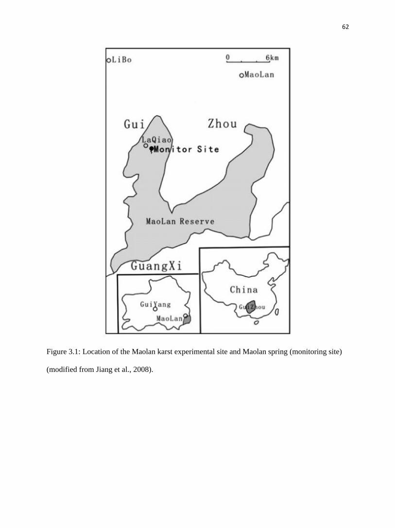
62
Figure 3.1: Location of the Maolan karst experimental site and Maolan spring (monitoring site)
(modified from Jiang et al., 2008).
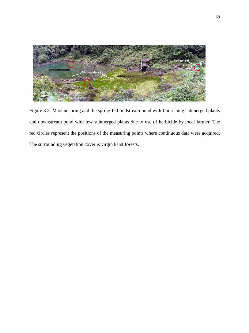
63
Figure 3.2: Maolan spring and the spring-fed midstream pond with flourishing submerged plants
and downstream pond with few submerged plants due to use of herbicide by local farmer. The
red circles represent the positions of the measuring points where continuous data were acquired.
The surrounding vegetation cover is virgin karst forests.
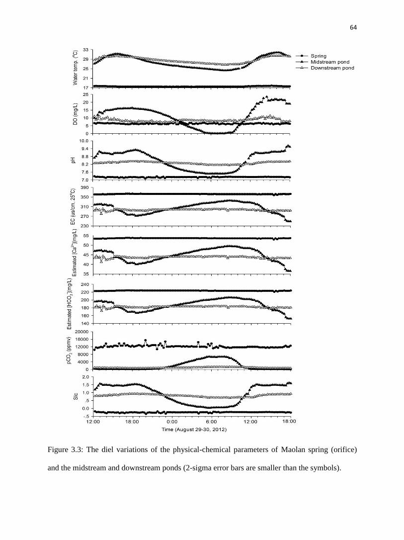
64
Figure 3.3: The diel variations of the physical-chemical parameters of Maolan spring (orifice)
and the midstream and downstream ponds (2-sigma error bars are smaller than the symbols).
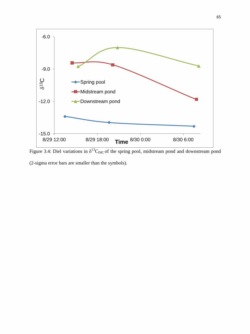
65
Figure 3.4: Diel variations in
13CDIC of the spring pool, midstream pond and downstream pond
(2-sigma error bars are smaller than the symbols).
-15.0
-12.0
-9.0
-6.0
8/29 12:00 8/29 18:00 8/30 0:00 8/30 6:00
13C
Time
Spring pool
Midstream pond
Downstream pond
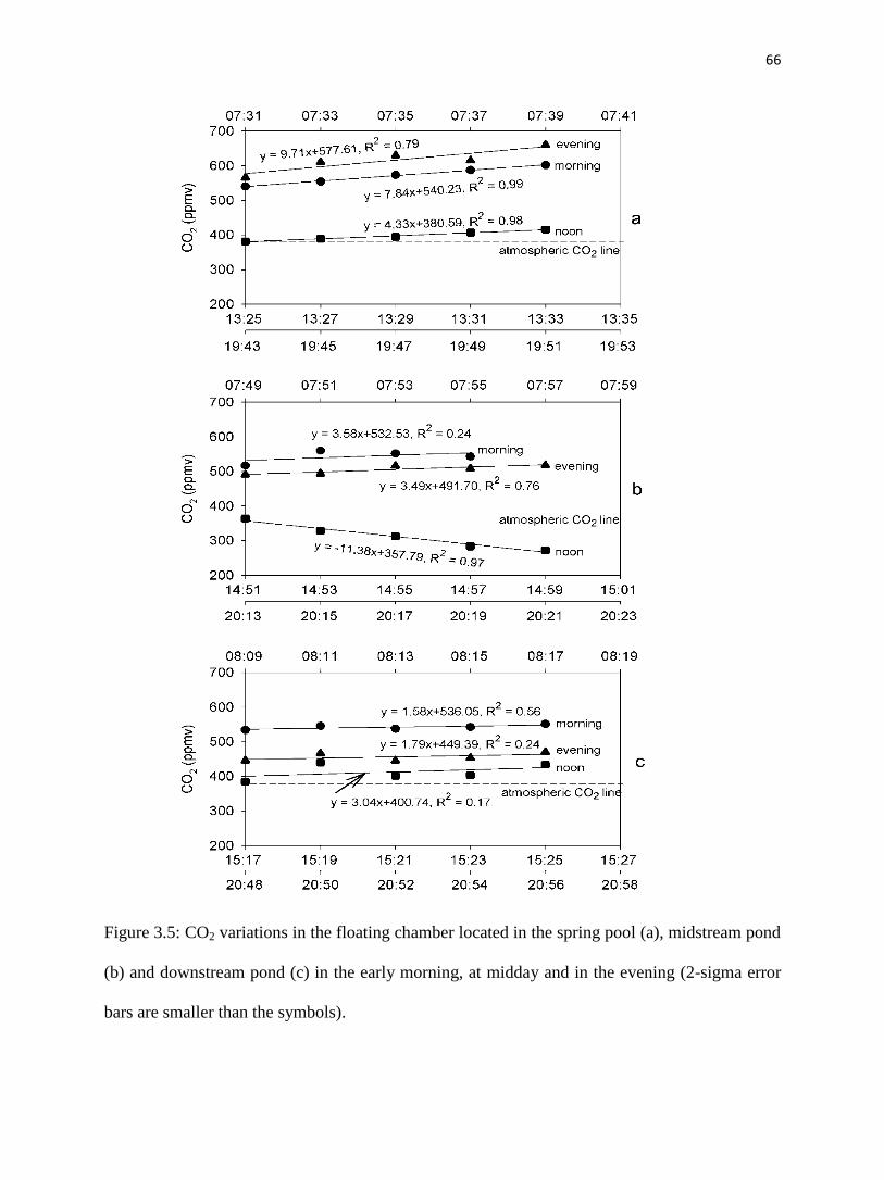
66
Figure 3.5: CO2 variations in the floating chamber located in the spring pool (a), midstream pond
(b) and downstream pond (c) in the early morning, at midday and in the evening (2-sigma error
bars are smaller than the symbols).
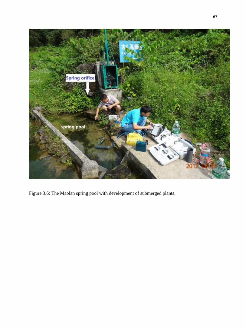
67
Figure 3.6: The Maolan spring pool with development of submerged plants.
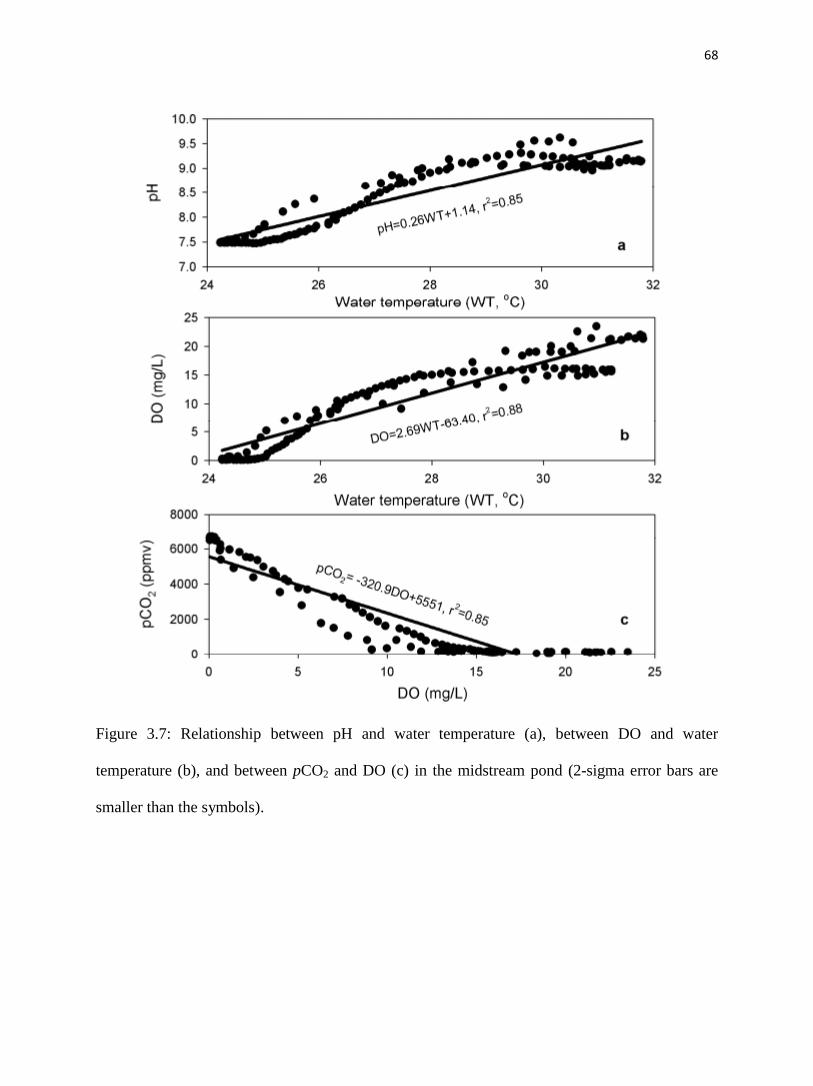
68
Figure 3.7: Relationship between pH and water temperature (a), between DO and water
temperature (b), and between pCO2 and DO (c) in the midstream pond (2-sigma error bars are
smaller than the symbols).
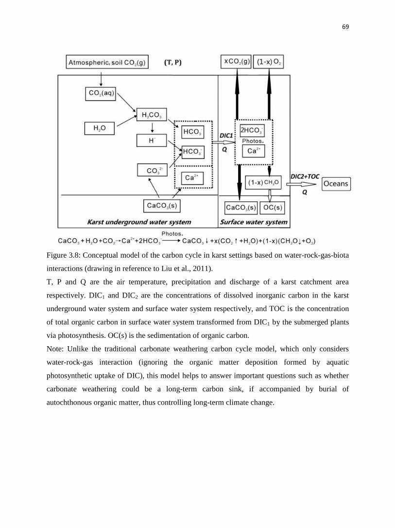
69
Figure 3.8: Conceptual model of the carbon cycle in karst settings based on water-rock-gas-biota
interactions (drawing in reference to Liu et al., 2011).
T, P and Q are the air temperature, precipitation and discharge of a karst catchment area
respectively. DIC1 and DIC2 are the concentrations of dissolved inorganic carbon in the karst
underground water system and surface water system respectively, and TOC is the concentration
of total organic carbon in surface water system transformed from DIC1 by the submerged plants
via photosynthesis. OC(s) is the sedimentation of organic carbon.
Note: Unlike the traditional carbonate weathering carbon cycle model, which only considers
water-rock-gas interaction (ignoring the organic matter deposition formed by aquatic
photosynthetic uptake of DIC), this model helps to answer important questions such as whether
carbonate weathering could be a long-term carbon sink, if accompanied by burial of
autochthonous organic matter, thus controlling long-term climate change.
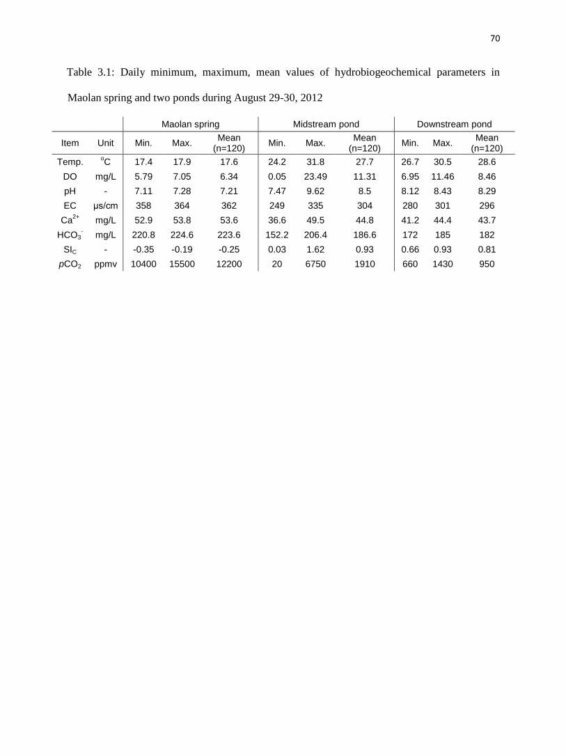
70
Table 3.1: Daily minimum, maximum, mean values of hydrobiogeochemical parameters in
Maolan spring and two ponds during August 29-30, 2012
Maolan spring Midstream pond Downstream pond
Item Unit Min. Max. Mean
(n=120) Min. Max.
Mean (n=120)
Min. Max. Mean
(n=120)
Temp. oC 17.4 17.9 17.6 24.2 31.8 27.7 26.7 30.5 28.6
DO mg/L 5.79 7.05 6.34 0.05 23.49 11.31 6.95 11.46 8.46
pH - 7.11 7.28 7.21 7.47 9.62 8.5 8.12 8.43 8.29
EC μs/cm 358 364 362 249 335 304 280 301 296
Ca2+
mg/L 52.9 53.8 53.6 36.6 49.5 44.8 41.2 44.4 43.7
HCO3- mg/L 220.8 224.6 223.6 152.2 206.4 186.6 172 185 182
SIC - -0.35 -0.19 -0.25 0.03 1.62 0.93 0.66 0.93 0.81
pCO2 ppmv 10400 15500 12200 20 6750 1910 660 1430 950
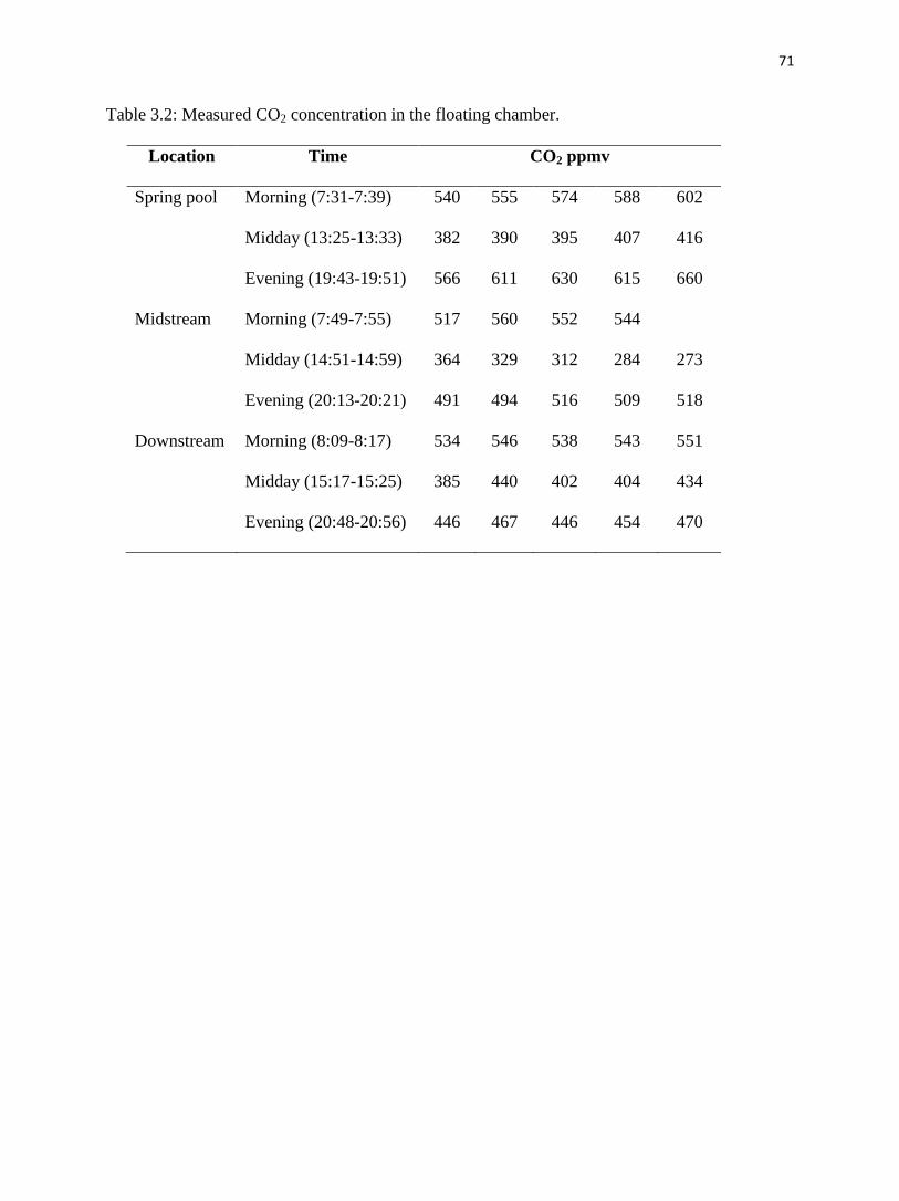
71
Table 3.2: Measured CO2 concentration in the floating chamber.
Location Time CO2 ppmv
Spring pool Morning (7:31-7:39) 540 555 574 588 602
Midday (13:25-13:33) 382 390 395 407 416
Evening (19:43-19:51) 566 611 630 615 660
Midstream Morning (7:49-7:55) 517 560 552 544
Midday (14:51-14:59) 364 329 312 284 273
Evening (20:13-20:21) 491 494 516 509 518
Downstream Morning (8:09-8:17) 534 546 538 543 551
Midday (15:17-15:25) 385 440 402 404 434
Evening (20:48-20:56) 446 467 446 454 470
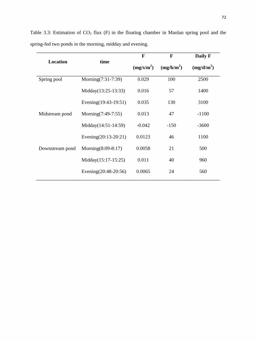
72
Table 3.3: Estimation of CO2 flux (F) in the floating chamber in Maolan spring pool and the
spring-fed two ponds in the morning, midday and evening.
Location time
F
(mg/s/m2)
F
(mg/h/m2)
Daily F
(mg/d/m2)
Spring pool Morning(7:31-7:39) 0.029 100 2500
Midday(13:25-13:33) 0.016 57 1400
Evening(19:43-19:51) 0.035 130 3100
Midstream pond Morning(7:49-7:55) 0.013 47 -1100
Midday(14:51-14:59) -0.042 -150 -3600
Evening(20:13-20:21) 0.0123 46 1100
Downstream pond Morning(8:09-8:17) 0.0058 21 500
Midday(15:17-15:25) 0.011 40 960
Evening(20:48-20:56) 0.0065 24 560

73
APPENDICIES
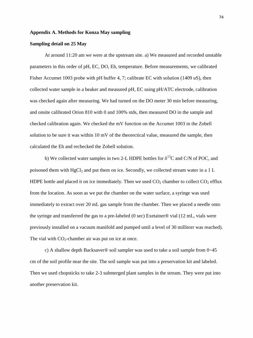
74
Appendix A. Methods for Konza May sampling
Sampling detail on 25 May
At around 11:20 am we were at the upstream site. a) We measured and recorded unstable
parameters in this order of pH, EC, DO, Eh, temperature. Before measurements, we calibrated
Fisher Accumet 1003 probe with pH buffer 4, 7; calibrate EC with solution (1409 uS), then
collected water sample in a beaker and measured pH, EC using pH/ATC electrode, calibration
was checked again after measuring. We had turned on the DO meter 30 min before measuring,
and onsite calibrated Orion 810 with 0 and 100% stds, then measured DO in the sample and
checked calibration again. We checked the mV function on the Accumet 1003 in the Zobell
solution to be sure it was within 10 mV of the theorectical value, measured the sample, then
calculated the Eh and rechecked the Zobell solution.
b) We collected water samples in two 2-L HDPE bottles for 13
C and C/N of POC, and
poisoned them with HgCl2 and put them on ice. Secondly, we collected stream water in a 1 L
HDPE bottle and placed it on ice immediately. Then we used CO2 chamber to collect CO2 efflux
from the location. As soon as we put the chamber on the water surface, a syringe was used
immediately to extract over 20 mL gas sample from the chamber. Then we placed a needle onto
the syringe and transferred the gas to a pre-labeled (0 sec) Exetainer® vial (12 mL, vials were
previously installed on a vacuum manifold and pumped until a level of 30 millitorr was reached).
The vial with CO2-chamber air was put on ice at once.
c) A shallow depth Backsaver® soil sampler was used to take a soil sample from 0~45
cm of the soil profile near the site. The soil sample was put into a preservation kit and labeled.
Then we used chopsticks to take 2-3 submerged plant samples in the stream. They were put into
another preservation kit.
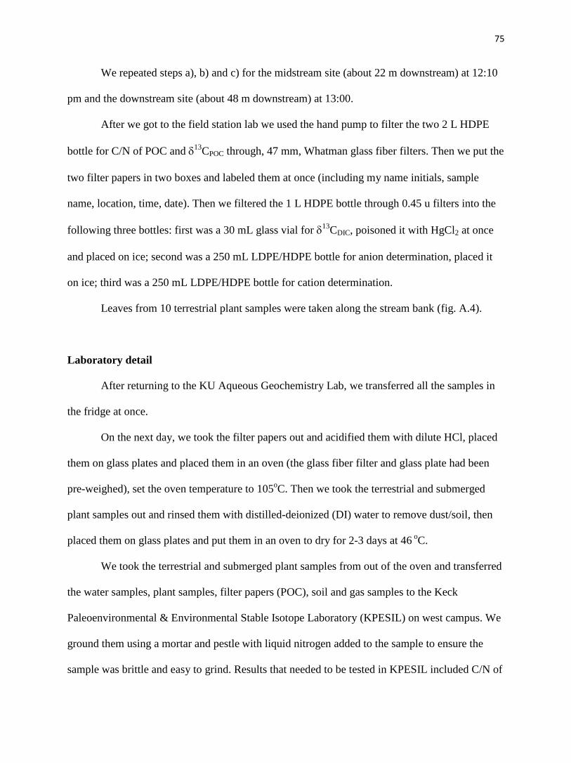
75
We repeated steps a), b) and c) for the midstream site (about 22 m downstream) at 12:10
pm and the downstream site (about 48 m downstream) at 13:00.
After we got to the field station lab we used the hand pump to filter the two 2 L HDPE
bottle for C/N of POC and 13
CPOC through, 47 mm, Whatman glass fiber filters. Then we put the
two filter papers in two boxes and labeled them at once (including my name initials, sample
name, location, time, date). Then we filtered the 1 L HDPE bottle through 0.45 u filters into the
following three bottles: first was a 30 mL glass vial for 13
CDIC, poisoned it with HgCl2 at once
and placed on ice; second was a 250 mL LDPE/HDPE bottle for anion determination, placed it
on ice; third was a 250 mL LDPE/HDPE bottle for cation determination.
Leaves from 10 terrestrial plant samples were taken along the stream bank (fig. A.4).
Laboratory detail
After returning to the KU Aqueous Geochemistry Lab, we transferred all the samples in
the fridge at once.
On the next day, we took the filter papers out and acidified them with dilute HCl, placed
them on glass plates and placed them in an oven (the glass fiber filter and glass plate had been
pre-weighed), set the oven temperature to 105oC. Then we took the terrestrial and submerged
plant samples out and rinsed them with distilled-deionized (DI) water to remove dust/soil, then
placed them on glass plates and put them in an oven to dry for 2-3 days at 46 oC.
We took the terrestrial and submerged plant samples from out of the oven and transferred
the water samples, plant samples, filter papers (POC), soil and gas samples to the Keck
Paleoenvironmental & Environmental Stable Isotope Laboratory (KPESIL) on west campus. We
ground them using a mortar and pestle with liquid nitrogen added to the sample to ensure the
sample was brittle and easy to grind. Results that needed to be tested in KPESIL included C/N of
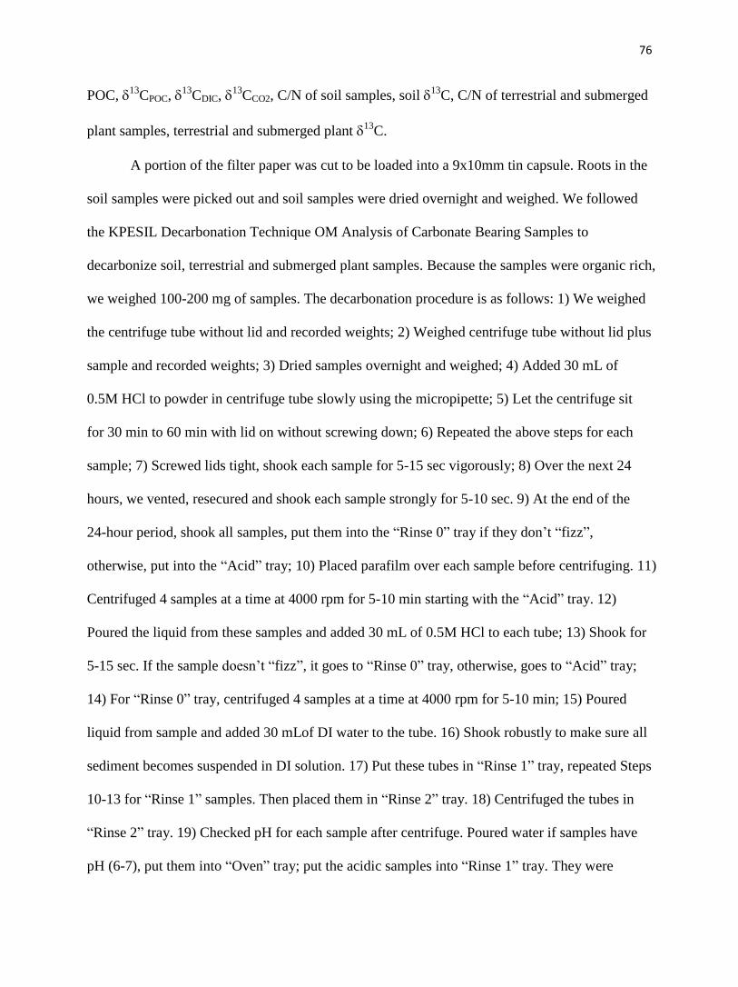
76
POC, 13
CPOC, 13
CDIC, 13
CCO2, C/N of soil samples, soil 13
C, C/N of terrestrial and submerged
plant samples, terrestrial and submerged plant 13
C.
A portion of the filter paper was cut to be loaded into a 9x10mm tin capsule. Roots in the
soil samples were picked out and soil samples were dried overnight and weighed. We followed
the KPESIL Decarbonation Technique OM Analysis of Carbonate Bearing Samples to
decarbonize soil, terrestrial and submerged plant samples. Because the samples were organic rich,
we weighed 100-200 mg of samples. The decarbonation procedure is as follows: 1) We weighed
the centrifuge tube without lid and recorded weights; 2) Weighed centrifuge tube without lid plus
sample and recorded weights; 3) Dried samples overnight and weighed; 4) Added 30 mL of
0.5M HCl to powder in centrifuge tube slowly using the micropipette; 5) Let the centrifuge sit
for 30 min to 60 min with lid on without screwing down; 6) Repeated the above steps for each
sample; 7) Screwed lids tight, shook each sample for 5-15 sec vigorously; 8) Over the next 24
hours, we vented, resecured and shook each sample strongly for 5-10 sec. 9) At the end of the
24-hour period, shook all samples, put them into the “Rinse 0” tray if they don’t “fizz”,
otherwise, put into the “Acid” tray; 10) Placed parafilm over each sample before centrifuging. 11)
Centrifuged 4 samples at a time at 4000 rpm for 5-10 min starting with the “Acid” tray. 12)
Poured the liquid from these samples and added 30 mL of 0.5M HCl to each tube; 13) Shook for
5-15 sec. If the sample doesn’t “fizz”, it goes to “Rinse 0” tray, otherwise, goes to “Acid” tray;
14) For “Rinse 0” tray, centrifuged 4 samples at a time at 4000 rpm for 5-10 min; 15) Poured
liquid from sample and added 30 mLof DI water to the tube. 16) Shook robustly to make sure all
sediment becomes suspended in DI solution. 17) Put these tubes in “Rinse 1” tray, repeated Steps
10-13 for “Rinse 1” samples. Then placed them in “Rinse 2” tray. 18) Centrifuged the tubes in
“Rinse 2” tray. 19) Checked pH for each sample after centrifuge. Poured water if samples have
pH (6-7), put them into “Oven” tray; put the acidic samples into “Rinse 1” tray. They were
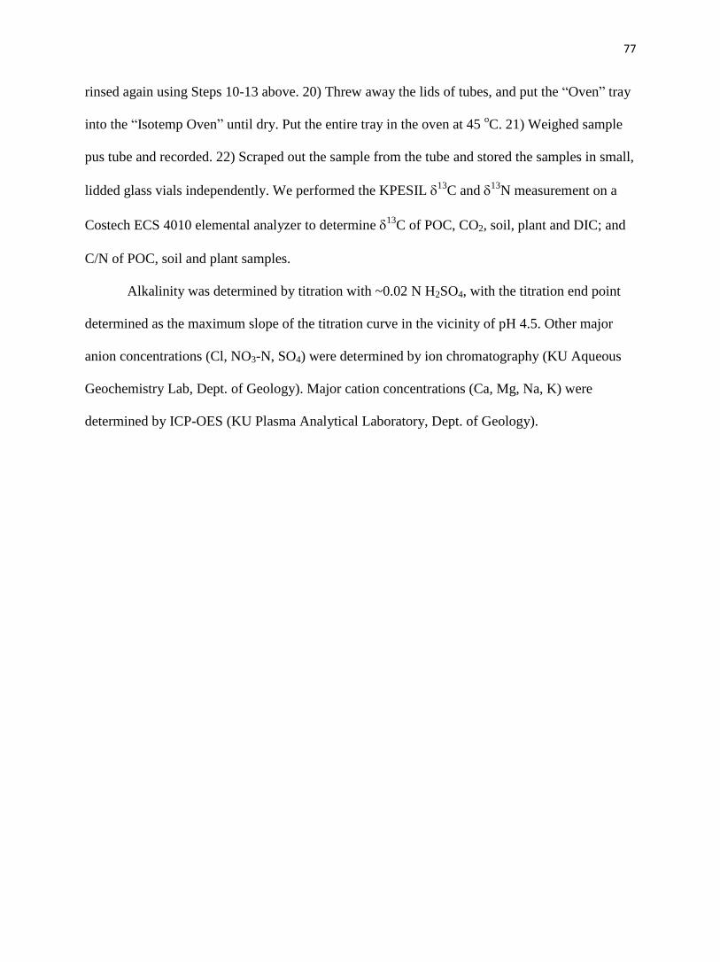
77
rinsed again using Steps 10-13 above. 20) Threw away the lids of tubes, and put the “Oven” tray
into the “Isotemp Oven” until dry. Put the entire tray in the oven at 45 oC. 21) Weighed sample
pus tube and recorded. 22) Scraped out the sample from the tube and stored the samples in small,
lidded glass vials independently. We performed the KPESIL 13
C and 13
N measurement on a
Costech ECS 4010 elemental analyzer to determine 13
C of POC, CO2, soil, plant and DIC; and
C/N of POC, soil and plant samples.
Alkalinity was determined by titration with ~0.02 N H2SO4, with the titration end point
determined as the maximum slope of the titration curve in the vicinity of pH 4.5. Other major
anion concentrations (Cl, NO3-N, SO4) were determined by ion chromatography (KU Aqueous
Geochemistry Lab, Dept. of Geology). Major cation concentrations (Ca, Mg, Na, K) were
determined by ICP-OES (KU Plasma Analytical Laboratory, Dept. of Geology).
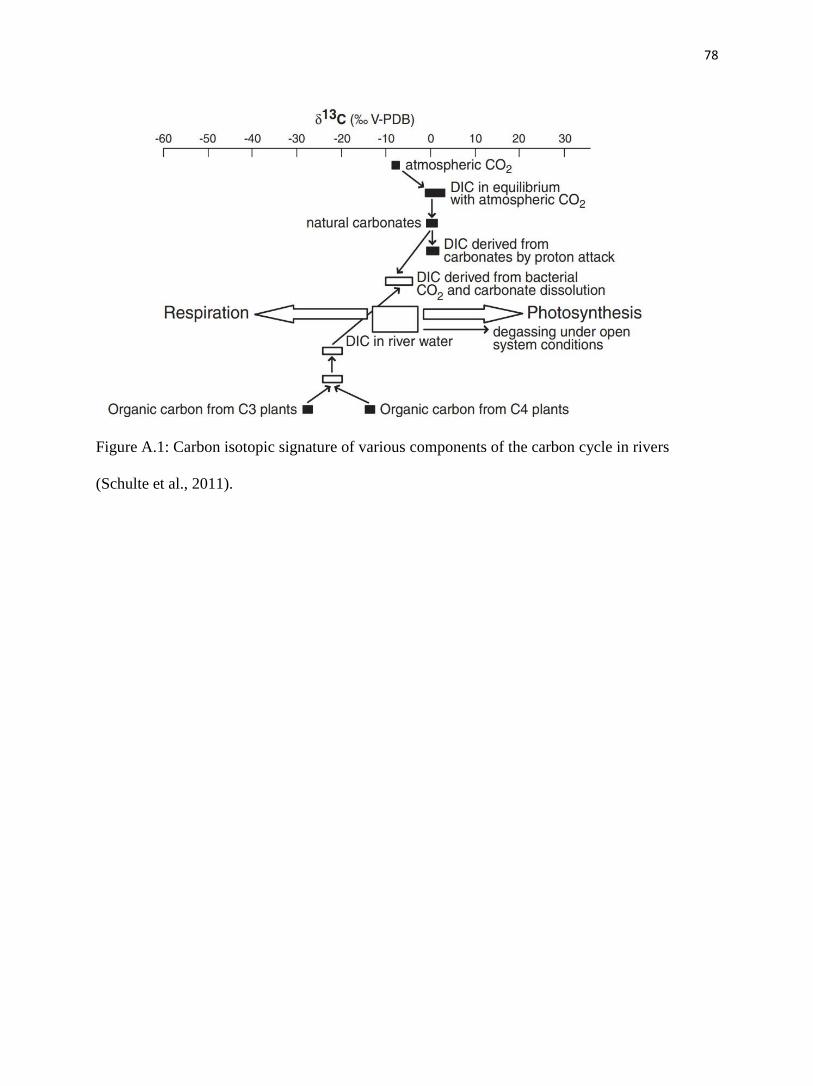
78
Figure A.1: Carbon isotopic signature of various components of the carbon cycle in rivers
(Schulte et al., 2011).
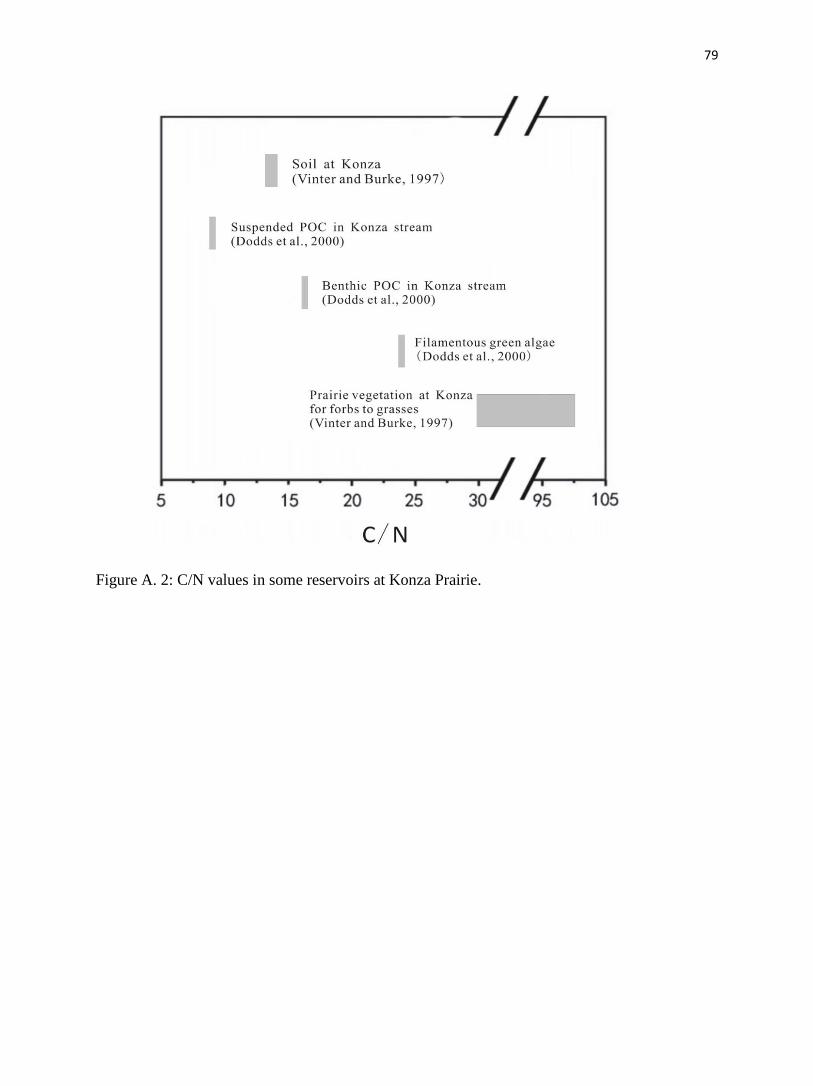
79
Figure A. 2: C/N values in some reservoirs at Konza Prairie.
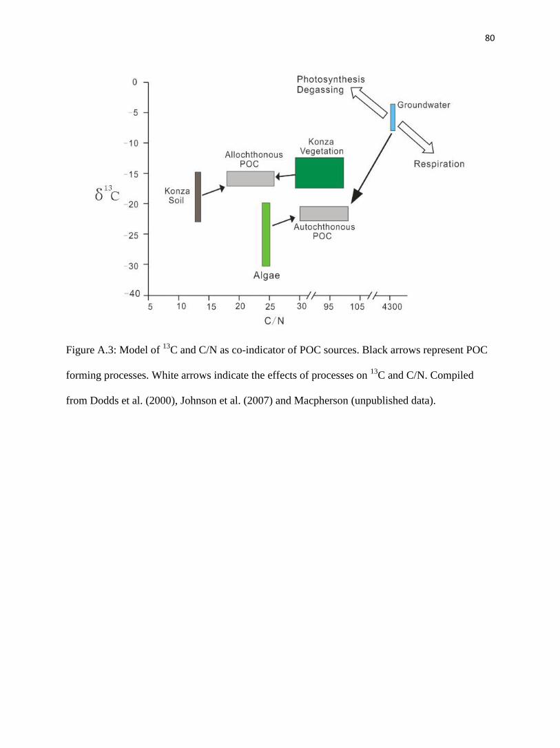
80
Figure A.3: Model of 13
C and C/N as co-indicator of POC sources. Black arrows represent POC
forming processes. White arrows indicate the effects of processes on 13
C and C/N. Compiled
from Dodds et al. (2000), Johnson et al. (2007) and Macpherson (unpublished data).
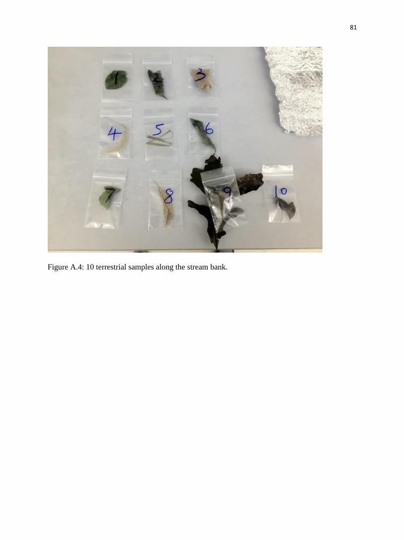
81
Figure A.4: 10 terrestrial samples along the stream bank.
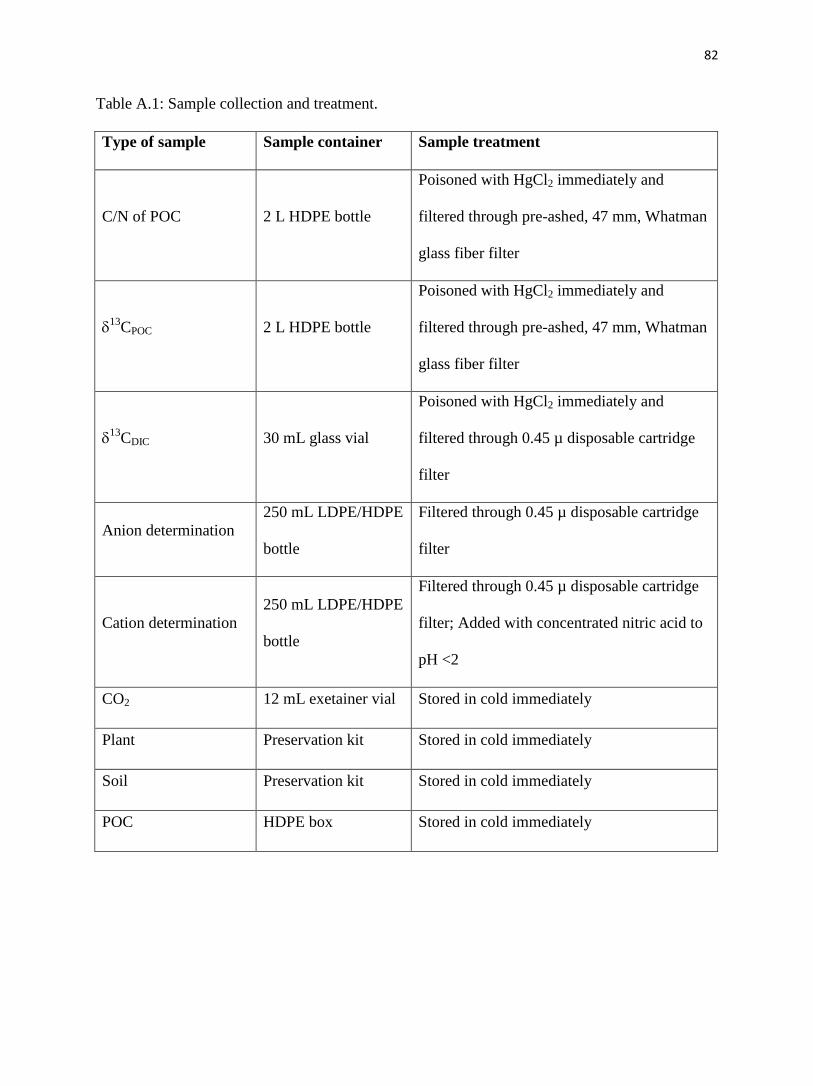
82
Table A.1: Sample collection and treatment.
Type of sample Sample container Sample treatment
C/N of POC 2 L HDPE bottle
Poisoned with HgCl2 immediately and
filtered through pre-ashed, 47 mm, Whatman
glass fiber filter
13
CPOC 2 L HDPE bottle
Poisoned with HgCl2 immediately and
filtered through pre-ashed, 47 mm, Whatman
glass fiber filter
13
CDIC 30 mL glass vial
Poisoned with HgCl2 immediately and
filtered through 0.45 µ disposable cartridge
filter
Anion determination
250 mL LDPE/HDPE
bottle
Filtered through 0.45 µ disposable cartridge
filter
Cation determination
250 mL LDPE/HDPE
bottle
Filtered through 0.45 µ disposable cartridge
filter; Added with concentrated nitric acid to
pH <2
CO2 12 mL exetainer vial Stored in cold immediately
Plant Preservation kit Stored in cold immediately
Soil Preservation kit Stored in cold immediately
POC HDPE box Stored in cold immediately
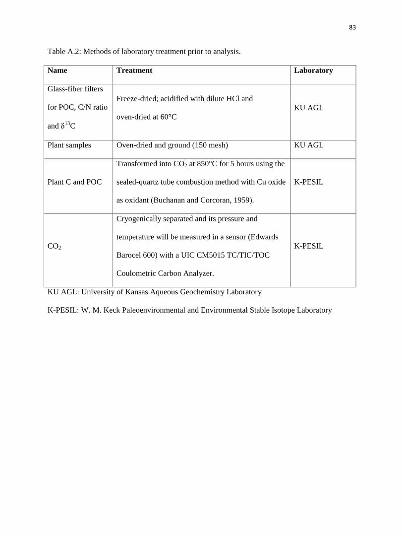
83
Table A.2: Methods of laboratory treatment prior to analysis.
Name Treatment Laboratory
Glass-fiber filters
for POC, C/N ratio
and 13
C
Freeze-dried; acidified with dilute HCl and
oven-dried at 60°C
KU AGL
Plant samples Oven-dried and ground (150 mesh) KU AGL
Plant C and POC
Transformed into CO2 at 850°C for 5 hours using the
sealed-quartz tube combustion method with Cu oxide
as oxidant (Buchanan and Corcoran, 1959).
K-PESIL
CO2
Cryogenically separated and its pressure and
temperature will be measured in a sensor (Edwards
Barocel 600) with a UIC CM5015 TC/TIC/TOC
Coulometric Carbon Analyzer.
K-PESIL
KU AGL: University of Kansas Aqueous Geochemistry Laboratory
K-PESIL: W. M. Keck Paleoenvironmental and Environmental Stable Isotope Laboratory
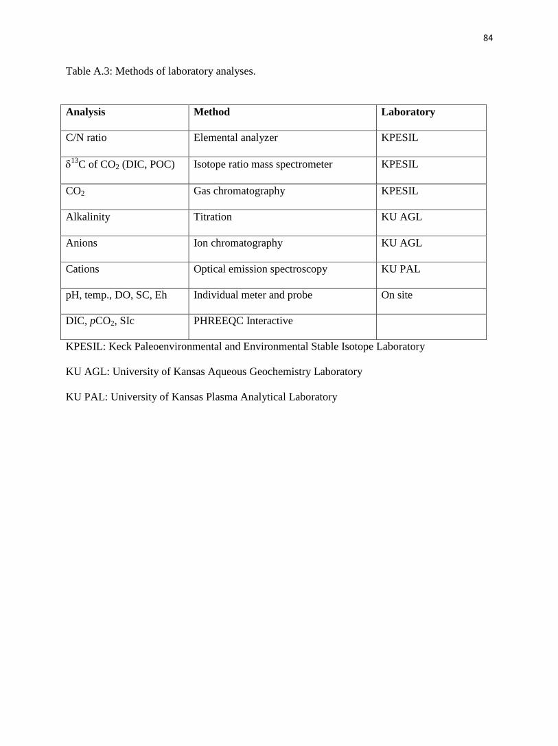
84
Table A.3: Methods of laboratory analyses.
KPESIL: Keck Paleoenvironmental and Environmental Stable Isotope Laboratory
KU AGL: University of Kansas Aqueous Geochemistry Laboratory
KU PAL: University of Kansas Plasma Analytical Laboratory
Analysis Method Laboratory
C/N ratio Elemental analyzer KPESIL
13
C of CO2 (DIC, POC) Isotope ratio mass spectrometer KPESIL
CO2 Gas chromatography KPESIL
Alkalinity Titration KU AGL
Anions Ion chromatography KU AGL
Cations Optical emission spectroscopy KU PAL
pH, temp., DO, SC, Eh Individual meter and probe On site
DIC, pCO2, SIc PHREEQC Interactive
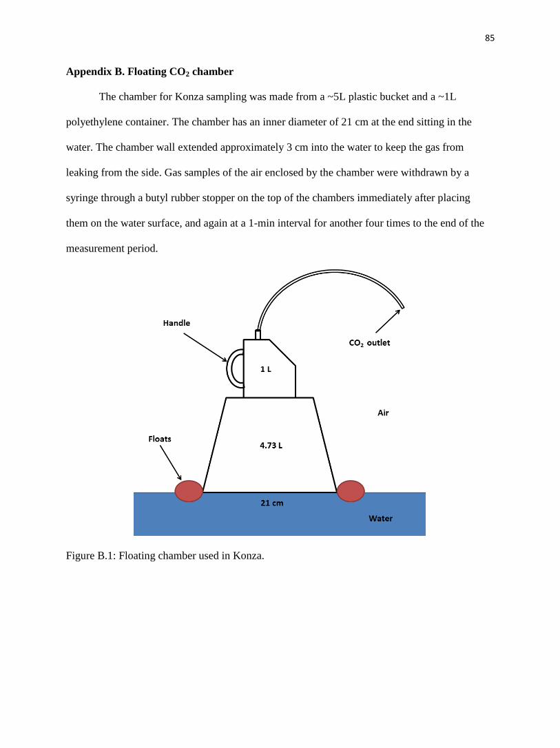
85
Appendix B. Floating CO2 chamber
The chamber for Konza sampling was made from a ~5L plastic bucket and a ~1L
polyethylene container. The chamber has an inner diameter of 21 cm at the end sitting in the
water. The chamber wall extended approximately 3 cm into the water to keep the gas from
leaking from the side. Gas samples of the air enclosed by the chamber were withdrawn by a
syringe through a butyl rubber stopper on the top of the chambers immediately after placing
them on the water surface, and again at a 1-min interval for another four times to the end of the
measurement period.
Figure B.1: Floating chamber used in Konza.
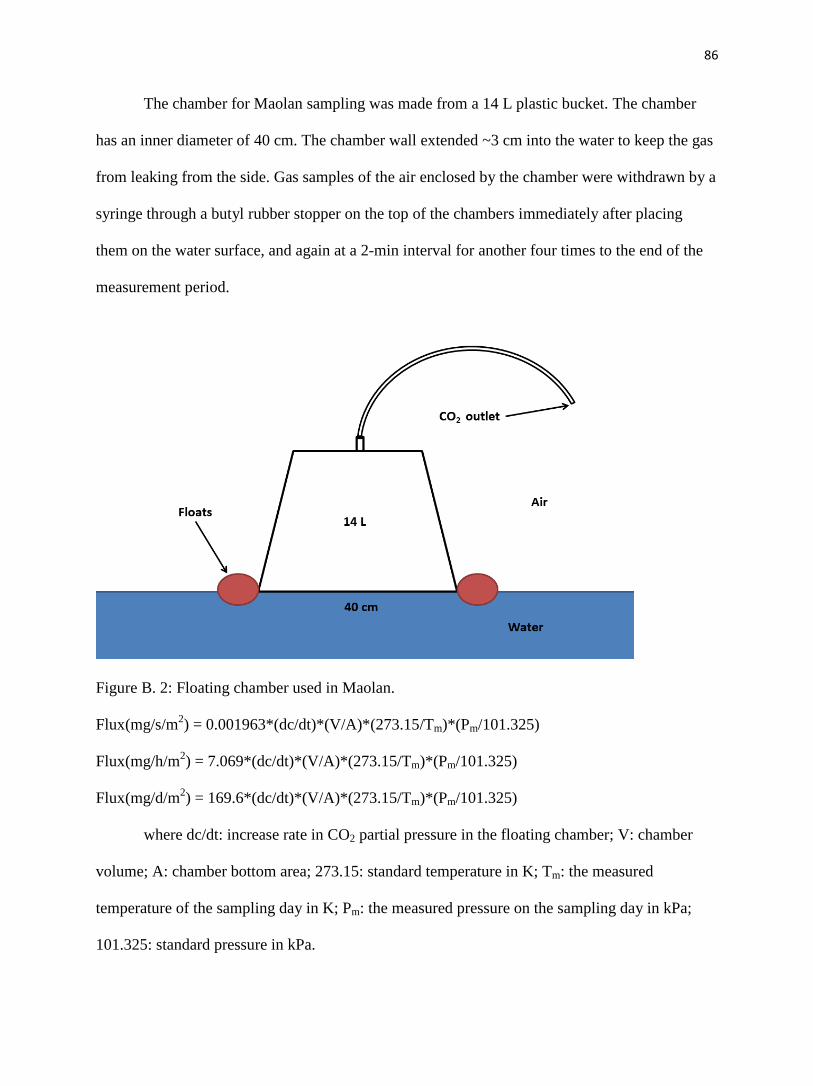
86
The chamber for Maolan sampling was made from a 14 L plastic bucket. The chamber
has an inner diameter of 40 cm. The chamber wall extended ~3 cm into the water to keep the gas
from leaking from the side. Gas samples of the air enclosed by the chamber were withdrawn by a
syringe through a butyl rubber stopper on the top of the chambers immediately after placing
them on the water surface, and again at a 2-min interval for another four times to the end of the
measurement period.
Figure B. 2: Floating chamber used in Maolan.
Flux(mg/s/m2) = 0.001963*(dc/dt)*(V/A)*(273.15/Tm)*(Pm/101.325)
Flux(mg/h/m2) = 7.069*(dc/dt)*(V/A)*(273.15/Tm)*(Pm/101.325)
Flux(mg/d/m2) = 169.6*(dc/dt)*(V/A)*(273.15/Tm)*(Pm/101.325)
where dc/dt: increase rate in CO2 partial pressure in the floating chamber; V: chamber
volume; A: chamber bottom area; 273.15: standard temperature in K; Tm: the measured
temperature of the sampling day in K; Pm: the measured pressure on the sampling day in kPa;
101.325: standard pressure in kPa.
87
Appendix C. Long-term data analysis of Konza Prairie
Summary
This study continues and expands the work of Macpherson et al., (2008), who proposed
several hypotheses clarifying the increasing trend of shallow groundwater pCO2 at the Konza
Prairie LTER Site. Approximately monthly data over 20 years at the Konza Prairie in
northeastern Kansas shows strong connection between the annual cycles of air temperature,
precipitation, atmosphere pCO2, and groundwater pCO2 trends.
The seasonal trend of groundwater pCO2 mimics the temperature annual cycle because
temperature governs soil CO2 (the main source of groundwater CO2) by controlling the terrestrial
vegetation photosynthesis and root respiration. Kings Creek discharge shows abrupt variation
with precipitation, while there is three months of lag-time between groundwater CO2 maximum
and precipitation. The delay may be the delivering time of soil CO2 to the groundwater initiated
by storm events. Analysis from SPSS shows that atmospheric temperature is the greatest factor
regulating groundwater CO2. NPP shows some fluctuation with precipitation and air temperature.
But it seems to be non-responsive to other parameters and shows no significant pattern over the
study period at the Konza Prairie. Results show that groundwater CO2 has increased about 29%
from 1990 to 2009 at Konza Prairie, which is greater than the 9% increase in atmospheric CO2
over the same time period, indicating that shallow groundwater is performing as a CO2 sink.
C.1. Introduction
The Konza Prairie Long-Term Ecological Research (LTER) Site and Biological Station
(Konza), located in the northeastern Kansas, is isolated from cities and agriculture croplands.
Thus, Konza is an ideal place to study natural grassland communities and ecosystems. Long-term
studies would serve to understand how the global change phenomena including land-use and
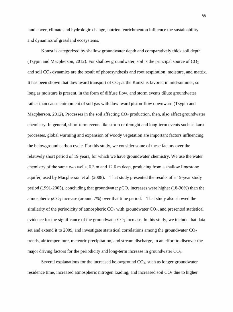
88
land cover, climate and hydrologic change, nutrient enrichmenton influence the sustainability
and dynamics of grassland ecosystems.
Konza is categorized by shallow groundwater depth and comparatively thick soil depth
(Tsypin and Macpherson, 2012). For shallow groundwater, soil is the principal source of CO2
and soil CO2 dynamics are the result of photosynthesis and root respiration, moisture, and matrix.
It has been shown that downward transport of CO2 at the Konza is favored in mid-summer, so
long as moisture is present, in the form of diffuse flow, and storm events dilute groundwater
rather than cause entrapment of soil gas with downward piston-flow downward (Tsypin and
Macpherson, 2012). Processes in the soil affecting CO2 production, then, also affect groundwater
chemistry. In general, short-term events like storm or drought and long-term events such as karst
processes, global warming and expansion of woody vegetation are important factors influencing
the belowground carbon cycle. For this study, we consider some of these factors over the
relatively short period of 19 years, for which we have groundwater chemistry. We use the water
chemistry of the same two wells, 6.3 m and 12.6 m deep, producing from a shallow limestone
aquifer, used by Macpherson et al. (2008). That study presented the results of a 15-year study
period (1991-2005), concluding that groundwater pCO2 increases were higher (18-36%) than the
atmospheric pCO2 increase (around 7%) over that time period. That study also showed the
similarity of the periodicity of atmospheric CO2 with groundwater CO2, and presented statistical
evidence for the significance of the groundwater CO2 increase. In this study, we include that data
set and extend it to 2009, and investigate statistical correlations among the groundwater CO2
trends, air temperature, meteoric precipitation, and stream discharge, in an effort to discover the
major driving factors for the periodicity and long-term increase in groundwater CO2.
Several explanations for the increased belowground CO2, such as longer groundwater
residence time, increased atmospheric nitrogen loading, and increased soil CO2 due to higher
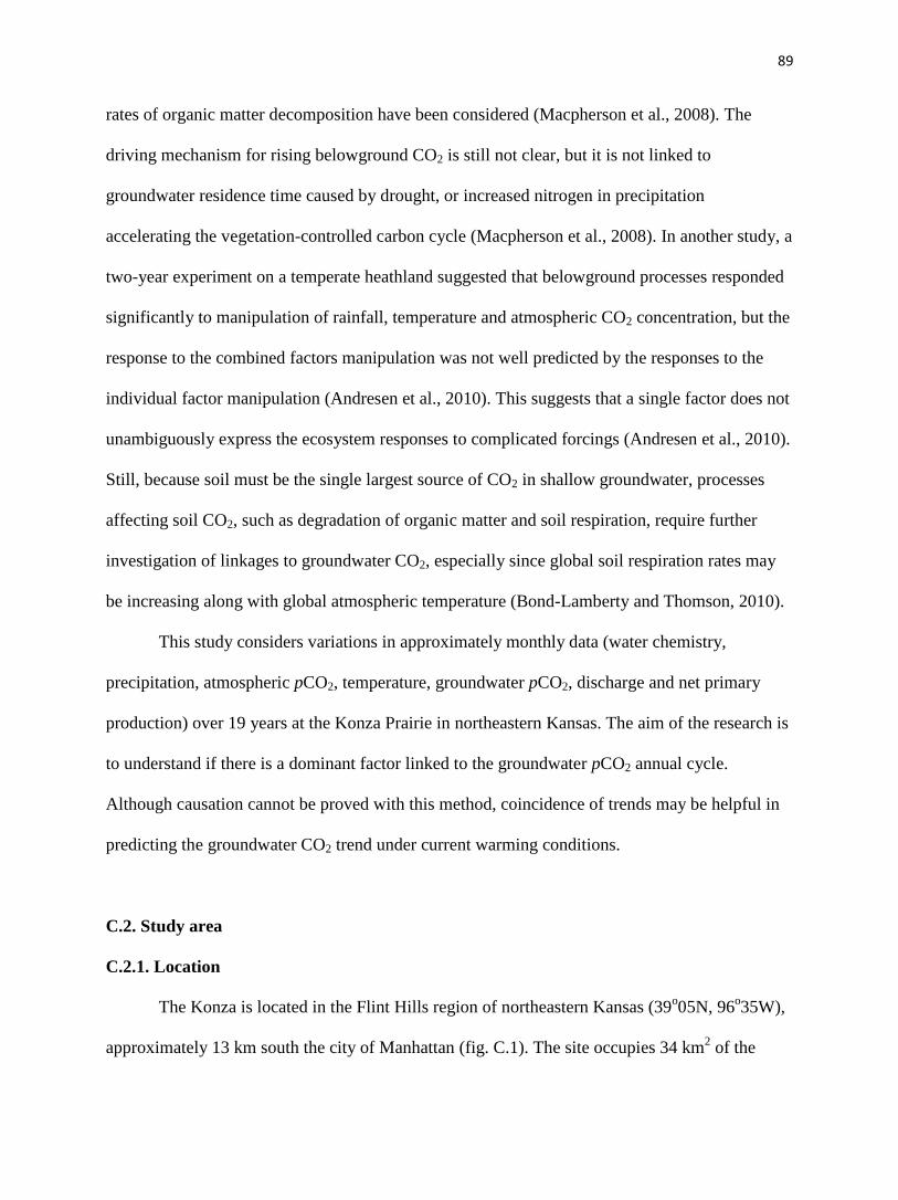
89
rates of organic matter decomposition have been considered (Macpherson et al., 2008). The
driving mechanism for rising belowground CO2 is still not clear, but it is not linked to
groundwater residence time caused by drought, or increased nitrogen in precipitation
accelerating the vegetation-controlled carbon cycle (Macpherson et al., 2008). In another study, a
two-year experiment on a temperate heathland suggested that belowground processes responded
significantly to manipulation of rainfall, temperature and atmospheric CO2 concentration, but the
response to the combined factors manipulation was not well predicted by the responses to the
individual factor manipulation (Andresen et al., 2010). This suggests that a single factor does not
unambiguously express the ecosystem responses to complicated forcings (Andresen et al., 2010).
Still, because soil must be the single largest source of CO2 in shallow groundwater, processes
affecting soil CO2, such as degradation of organic matter and soil respiration, require further
investigation of linkages to groundwater CO2, especially since global soil respiration rates may
be increasing along with global atmospheric temperature (Bond-Lamberty and Thomson, 2010).
This study considers variations in approximately monthly data (water chemistry,
precipitation, atmospheric pCO2, temperature, groundwater pCO2, discharge and net primary
production) over 19 years at the Konza Prairie in northeastern Kansas. The aim of the research is
to understand if there is a dominant factor linked to the groundwater pCO2 annual cycle.
Although causation cannot be proved with this method, coincidence of trends may be helpful in
predicting the groundwater CO2 trend under current warming conditions.
C.2. Study area
C.2.1. Location
The Konza is located in the Flint Hills region of northeastern Kansas (39o05N, 96
o35W),
approximately 13 km south the city of Manhattan (fig. C.1). The site occupies 34 km2 of the
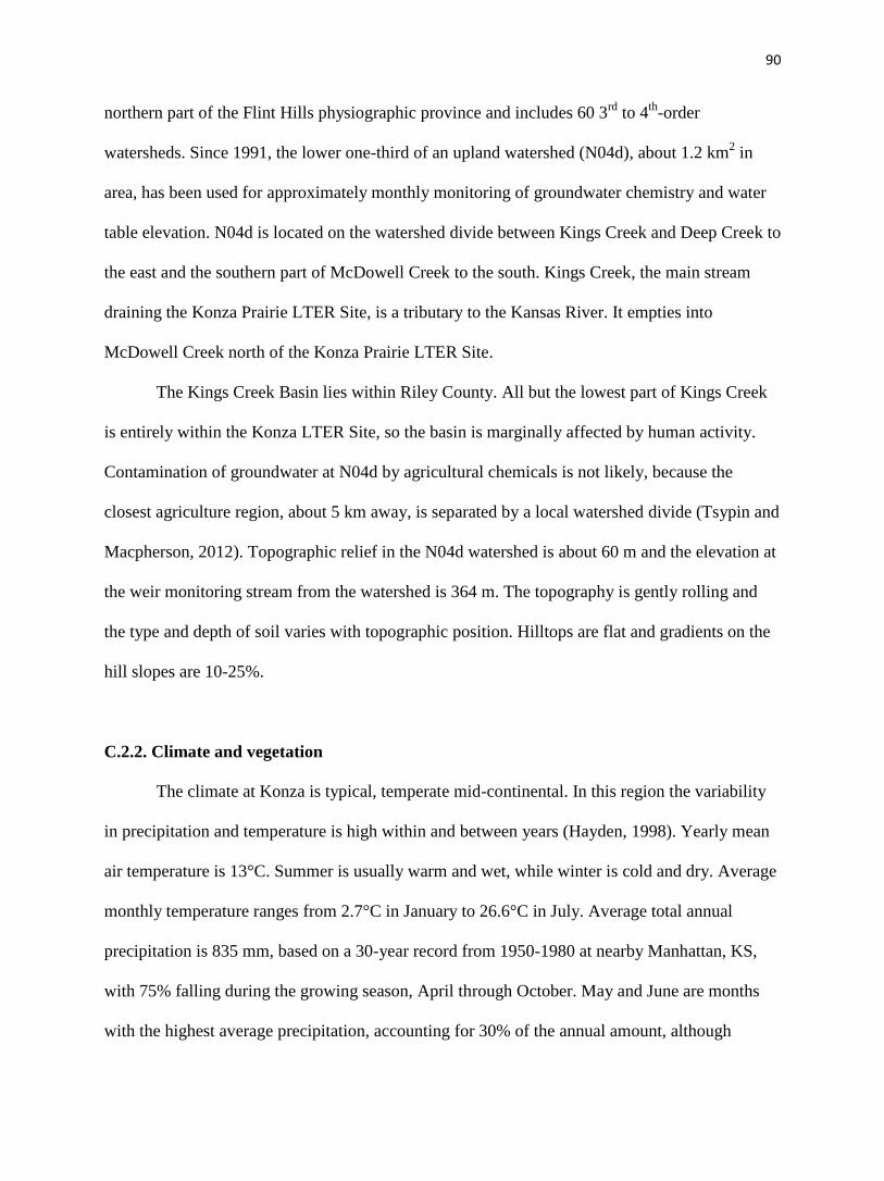
90
northern part of the Flint Hills physiographic province and includes 60 3rd
to 4th
-order
watersheds. Since 1991, the lower one-third of an upland watershed (N04d), about 1.2 km2 in
area, has been used for approximately monthly monitoring of groundwater chemistry and water
table elevation. N04d is located on the watershed divide between Kings Creek and Deep Creek to
the east and the southern part of McDowell Creek to the south. Kings Creek, the main stream
draining the Konza Prairie LTER Site, is a tributary to the Kansas River. It empties into
McDowell Creek north of the Konza Prairie LTER Site.
The Kings Creek Basin lies within Riley County. All but the lowest part of Kings Creek
is entirely within the Konza LTER Site, so the basin is marginally affected by human activity.
Contamination of groundwater at N04d by agricultural chemicals is not likely, because the
closest agriculture region, about 5 km away, is separated by a local watershed divide (Tsypin and
Macpherson, 2012). Topographic relief in the N04d watershed is about 60 m and the elevation at
the weir monitoring stream from the watershed is 364 m. The topography is gently rolling and
the type and depth of soil varies with topographic position. Hilltops are flat and gradients on the
hill slopes are 10-25%.
C.2.2. Climate and vegetation
The climate at Konza is typical, temperate mid-continental. In this region the variability
in precipitation and temperature is high within and between years (Hayden, 1998). Yearly mean
air temperature is 13°C. Summer is usually warm and wet, while winter is cold and dry. Average
monthly temperature ranges from 2.7°C in January to 26.6°C in July. Average total annual
precipitation is 835 mm, based on a 30-year record from 1950-1980 at nearby Manhattan, KS,
with 75% falling during the growing season, April through October. May and June are months
with the highest average precipitation, accounting for 30% of the annual amount, although
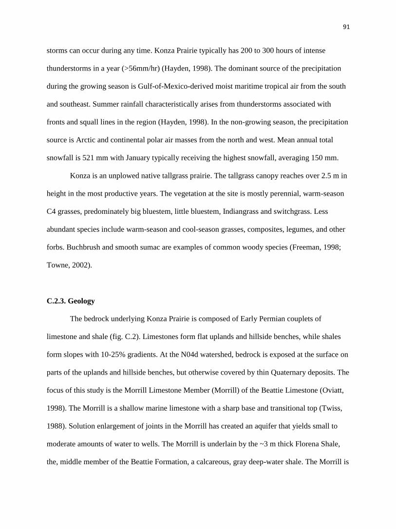
91
storms can occur during any time. Konza Prairie typically has 200 to 300 hours of intense
thunderstorms in a year (>56mm/hr) (Hayden, 1998). The dominant source of the precipitation
during the growing season is Gulf-of-Mexico-derived moist maritime tropical air from the south
and southeast. Summer rainfall characteristically arises from thunderstorms associated with
fronts and squall lines in the region (Hayden, 1998). In the non-growing season, the precipitation
source is Arctic and continental polar air masses from the north and west. Mean annual total
snowfall is 521 mm with January typically receiving the highest snowfall, averaging 150 mm.
Konza is an unplowed native tallgrass prairie. The tallgrass canopy reaches over 2.5 m in
height in the most productive years. The vegetation at the site is mostly perennial, warm-season
C4 grasses, predominately big bluestem, little bluestem, Indiangrass and switchgrass. Less
abundant species include warm-season and cool-season grasses, composites, legumes, and other
forbs. Buchbrush and smooth sumac are examples of common woody species (Freeman, 1998;
Towne, 2002).
C.2.3. Geology
The bedrock underlying Konza Prairie is composed of Early Permian couplets of
limestone and shale (fig. C.2). Limestones form flat uplands and hillside benches, while shales
form slopes with 10-25% gradients. At the N04d watershed, bedrock is exposed at the surface on
parts of the uplands and hillside benches, but otherwise covered by thin Quaternary deposits. The
focus of this study is the Morrill Limestone Member (Morrill) of the Beattie Limestone (Oviatt,
1998). The Morrill is a shallow marine limestone with a sharp base and transitional top (Twiss,
1988). Solution enlargement of joints in the Morrill has created an aquifer that yields small to
moderate amounts of water to wells. The Morrill is underlain by the ~3 m thick Florena Shale,
the, middle member of the Beattie Formation, a calcareous, gray deep-water shale. The Morrill is
92
overlain by the ~4.5 m thick Stearns Shale, a calcareous, terrigenous to marine shale (Zeller,
1968).
C.2.4. Soils
Soils of Konza are generally poor with carbonate and has low to moderate cation
exchange capacities (typically less than 40 meq/100g) (Ransom et al., 1998). The soils are less
than 1 m thick, evolving on loess, limestone and shale (Macpherson et al., 2008). Soils at N04d
watershed are relatively deep and temperately well-drained. The moderately permeable soils are
located on foot slopes and valley bottoms. The organic content declined with depth from 6% to
lower than 1%. The clay content ranges from 26 to 39%, silt from 37 to 57%, and sand from 7 to
40%. Soils commonly contain low amount of nutrients (3.5-6.0 ug/g available P, 265-285 ug/g
K, and 2.0-6.0 ug/g NO3-N) (Wehmueller et al., 2005).
C.2.5. Hydrogeology
The neo-karst aquifers include the Morrill Limestone Member of the Beattie Limstone
and the upper and lower portions of the Eiss Limestone Member of the Bader Limestone
(Macpherson, 1996). Thus, the aquifers are like sandwich (White, 1969). The aquifers in this
region are the 1-2 m thick limestone layers and the alluvial deposits, displaying secondary
porosity (Macpherson et al., 2008). The conductivities of the aquifers range from 10-8
to 10-3
m/s
(Pomes, 1995). The aquitards are the thicker shale layers.
The connection between surface water and groundwater is fairly rapid. Water level and
temperature change within a few hours after precipitation (Macpherson, 1996). During a single
sampling even in 1991, the tritium levels of groundwater are similar to meteoric precipitation
(Macpherson, 1992). Water level oscillates on a diel cycle with ~1 cm during prolonged dry
93
times in the growing season. Water level starts to decrease soon after sunrise, and rises again
within a few hours after sunset (Kissing and Macpherson, 2006).
The water chemistry of shallow groundwater (Ca2+
and HCO3- type) in the N04d
watershed is similar. Mg2+
is higher than in others in some units, with infrequent peaks of SO42-
.
The major control on groundwater pH and alkalinity is soil and bedrock carbonate weathering
(Macpherson, 1996).
C.3. Methods
The sampling took place in the northern part of the N04d watershed at Konza.
Observation wells are made of 5-cm diameter PVC casing with a 61-cm PVC slotted well screen
at the bottom. Steel well protectors protect the wells from controlled burning of the grassland
every four years and damage from bison. Two wells of the total of 35 wells in the watershed are
presented in this study. Well 4-6 Mor is 12.6 m deep, while well 3-5 is 6.3 m deep. Both wells
have been sampled continuously over the study period. We also present the relation between
stream samples collected at two locations nearest to the two wells. Sampling and chemical
analysis of groundwater and stream water occurred every four to six weeks. Details of sampling
and analysis methods are given in Macpherson et al. (2008).
C.3.1. Geochemical speciation modeling
Saturation index of carbonate minerals and dissolved inorganic carbon (DIC) species are
controlled by measured pH, alkalinity, and other dissolved species. Accurate pH measurements
are difficult at the study site because the limestones are low-yield aquifers and there is no power
available to run a pump. In this study, we follow the method in Macpherson et al. (2008). In brief,
pH was determined using the deliberate-degassing bottle technique (DDB pH; described in detail
94
in Macpherson, 2004) over a 1.67-year period to establish the annual cycle of calcite saturation.
This annual cycle was used, in all other years, to predict pH, pCO2 and other speciation with
PHREEQC Interactive 2.18.5570, applying the PHREEQC database (Parkhurst and Appelo,
1999). Headspace CO2 samples and field pH were determined in 2005 to investigate the validity
of using a repetitive SIc annual cycle. The measured results correspond well with predicted pCO2
and pH (Macpherson et al., 2008). The full chemical analysis and SIc are input in PHREEQC to
calculate the pH and the partial pressure of CO2.
C.3.2. Other data
Net primary production (NPP) data was acquired from the Konza LTER website
(www.konza.ksu.edu). At Konza, since 1989 aboveground NPP of Tallgrass Prairie has been
evaluated at maximum standing crop biomass on three watersheds (001d, 004b, 020b). Because
soils of N04d watershed are mostly Tully type, Tully soil was chosen as representative of the
N04d watershed. The NPP of live grass and forbs were combined for this study. Because the
NPP data of some of the months are missing and September is the only month for which NPP
data is available for all the years, only the NPP data for September is used here to represent the
value for each year.
C.3.3. Data analysis
In order to investigate the relationship between the parameters, it is necessary to examine
the lag time between two parameters (atmospheric CO2 and temperature; groundwater CO2 and
temperature; groundwater CO2 and atmospheric CO2, groundwater and meteoric precipitation).
We plot the data and correlate the peak values for each pair of parameters every year, and
estimate the lag time between the two peaks for each year. The average lag time each year for all
95
of the years is used as a lag time for those two parameters. Linear regression analysis in IBM
SPSS Statistics version 21 was used to evaluate the most significant parameters affecting
groundwater CO2. Groundwater CO2 was input as a dependent factor; air temperature,
atmospheric CO2 and meteoric precipitation were independent factors.
C.4. Results
C.4.1. Water chemistry
The study period for well 3-5 and well 4-6 is from 22 May 1990 to 7 July 2009. The
chemistry of water in the two wells is very similar. Total dissolved solids is composed primarily
of titration alkalinity, calcium and magnesium 82-94% (by weight). In well 3-5, alkalinity
occupies 87-99% of the total carbon. The pH ranges from 7.18 to 8.06 and TDS varies from 204
ppm to 388 ppm. For well 4-6, alkalinity makes up 84-99% of the total carbon, and pH fluctuates
between 7.03 and 8.01. TDS oscillates between 113 ppm to 375 ppm.
C.4.2. Atmospheric CO2
We use the time series of atmospheric CO2 recorded at the Mauna Loa Observatory
(MLO) situated on the island of Hawaii, because it was designed and has been continually
verified to capture the global average atmospheric CO2 trend. The atmospheric CO2 at MLO is
similar to that measured at Niwot Ridge, which is the nearest station to the Konza, but which has
a shorter record. The annual cycle of air CO2 at the MLO records the effects of photosynthesis
and respiration (Buermann et al., 2007) of the northern hemisphere biosphere, with a maximum
at the start of the growing season (April/May) and a minimum at the end of the growing season
(September/October) (fig. C.3).
96
C.4.3. Long-term trends
Fig. C.4 displays the long-term trends (year 1991 to 2009) of atmospheric pCO2,
groundwater pCO2 and alkalinity as HCO3- concentration for well 3-5. All of the parameters
increase at least 0.5% annually. Among them, groundwater pCO2 increases at the highest rate of
184 ppmv yearly, about 1.6%, while the atmospheric pCO2 increases at 1.84 ppmv annually
(0.5%). Alkalinity rises at a rate of 2.5 ppm/a. Atmospheric pCO2 increased by 9% from 1991 to
2009. Over the same time period, groundwater pCO2 increased by about 29%.
C.4.4. Groundwater pCO2 in relation to other physical parameters
Fig. C.3c shows that groundwater pCO2 fluctuates on an annual cycle, similar to the
atmospheric pCO2 cycle from year 1991 to 2009. However, there is about a 5 to 7-month lag
time between both their maxima and minima. The atmospheric pCO2 is normally the highest in
May, while the groundwater pCO2 usually reaches its maximum in September to October. The
atmospheric pCO2 decreases to its annual minimum in August to September, and groundwater
pCO2 decreases to its annual minimum in February to April.
Fig. C.3b displays that groundwater pCO2 corresponds very well with air temperature.
There is about two months lag time between the two parameters. Temperature increases to its
maximum value in July or August, and decreases to its lowest value in January.
Fig. C.5b shows that groundwater pCO2 and prairie precipitation follow similar annual
trends, with a time lag between them. The greatest amount of precipitation and discharge usually
occur in May to July. Generally, groundwater pCO2 increases with rising precipitation after
around three month.
97
C.4.5. Net primary production
Sala et al. (1988) estimated that annual aboveground NPP should average 510 g/m2 at
Konza. September is the month which NPP data are available in every year. The average NPP for
September is 420 g/m2, suggesting that NPP is normally the highest in early fall. NPP data for
September is used to represent the value for the year (fig. C.6). The NPP values range from 310
g/m2 to 538 g/m
2. There is no clear pattern of the NPP variation in relation to most of the
parameters, but the NPP commonly reaches its annual maximum after precipitation peaks (fig.
C.6b), and right after the air temperature peak (fig. C.6a). Aboveground NPP from 1991 to 2005
shows high variability and no statistically defensible trend.
C.5. Discussions
C.5.1. Implication from SPSS
Data of the three important factors (temperature, atmospheric CO2 and rainfall) that could
potentially influence the groundwater CO2 were input in SPSS to evaluate their significance. GW
CO2 is used as a dependent factor and the three parameters are as independent factors. “Enter
Method” in the Linear regression was chosen as the analytical method. After adjustment for the
lag time, we could generally correlate the data of each parameter to groundwater CO2. Results
show that rainfall has the highest sig. of 0.244, meaning it is the least influential factor, and
therefore should be excluded (normally if the sig. is less than 0.05 the effect is significant).
Temperature is the most dominant factor on groundwater CO2 with the lowest sig. (0.000),
followed by atmospheric CO2 (sig. 0.003)
98
C.5.2. Controlling factors on groundwater pCO2
C.5.2.1. Temperature and atmospheric pCO2
The oscillation of CO2 in the northern hemisphere reflects that photosynthesis uptaking
CO2 and respiration releasing CO2 are not simultaneous (Buermann et al., 2007). During the
summer, photosynthesis dominates over respiration in the northern hemisphere, resulting in
temporary storage of carbon in plant tissues along with a seasonal decline in atmospheric pCO2
levels. Therefore, the minimum atmospheric CO2 usually occurs in the early fall each year. On
the other hand, in winter, respiration by decomposers exceeds photosynthesis, because many
plants are dormant or leafless. Thus, atmospheric pCO2 returns to the highest levels. The
continuous CO2 increase in the atmosphere from 1991 to 2009 is mostly due to the burning of
fossil fuels, but a substantial portion has also resulted from the destruction of plant biomass. A
study points out that although fast-growing vegetation is found on most areas that are harvested,
the degree of carbon buildup does not match the rate of carbon loss during harvest, indicating a
net carbon transfer from biomass to atmosphere (Harmon et al., 1990). The increased
atmospheric pCO2 levels should not directly influence the groundwater pCO2, because
belowground pCO2 levels are normally one to two orders of magnitude higher than atmospheric
pCO2 (Macpherson et al., 2008). However, the groundwater pCO2 wave mimics the atmospheric
pCO2 and temperature cycles, and pCO2 build-up in the shallow aquifer is much faster than the
atmospheric pCO2 growth. Temperature and soil moisture are the main controls on terrestrial
vegetation photosynthesis (where light is not limiting) and root respiration. Therefore the
atmospheric pCO2 is related to air temperature, but only coincidentally related to groundwater
CO2 variation.
Belowground CO2 mostly derived from soil. PCO2 in the groundwater peaks during the
late fall, which is typical timing for shallow aquifers (Macpherson et al., 2008). Shallow soil
99
pCO2 peaks in the summer and there is a greater lag time to maximize CO2 with increasing soil
depth (Hendry et al., 1999; Tsypin and Macpherson, 2012). After the maximum, the soil CO2
declines due to moisture deficiency in the late summer and temperature drop beginning in the fall.
The CO2 begins decreasing earliest in the shallowest part of the soil and latest in the deepest part
(Tsypin and Macpherson, 2012). Groundwater pCO2 peaks in October, thus, the 2-3 months of
lag-time between the soil and groundwater CO2 may be the delivering time of soil CO2 to the
groundwater. This explains the out of phase between pCO2 in groundwater and temperature.
Temperature and soil moisture determine soil CO2 (the main source of groundwater CO2),
thus, the seasonal trend of temperature and groundwater pCO2 are similar (fig. C.3).
C.5.2.2. Prairie precipitation and Kings Creek discharge
The aqueous geochemistry in the aquifers is related to the history of precipitation events
(including magnitude) and temporal relation to earlier events (thus controlling groundwater
residence time). The connections between stream and groundwater at Konza Prairie are
complicated by sporadic and unevenly sized precipitation events (Gray et al., 1998).
At the Konza Prairie, Kings Creek discharge rate shows immediate variation, usually less
than a month, with precipitation (fig. C.5a). This rapid response has two implications. Firstly, it
suggests that the rain water travels quickly to the groundwater and discharges the stream as base
flow, which is a characteristic of karst systems. Secondly, intense precipitation events dominate
river and stream discharge when runoff is rapid (Milly et al., 2002). Therefore, groundwater
might be bypassed if intense precipitation events dominate stream discharge by rapid runoff.
Because rain water moves down from the large porous media, but most of the CO2 in the
soil is trapped in the small pores, thus, the CO2 downward movement is a lot slower than rain
water. Tsypin and Macpherson (2012) studied the extreme precipitation events at Konza Prairie
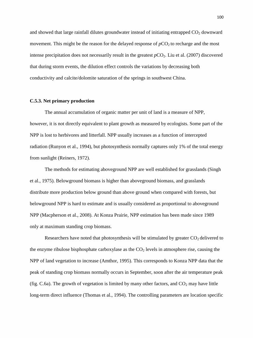
100
and showed that large rainfall dilutes groundwater instead of initiating entrapped CO2 downward
movement. This might be the reason for the delayed response of pCO2 to recharge and the most
intense precipitation does not necessarily result in the greatest pCO2. Liu et al. (2007) discovered
that during storm events, the dilution effect controls the variations by decreasing both
conductivity and calcite/dolomite saturation of the springs in southwest China.
C.5.3. Net primary production
The annual accumulation of organic matter per unit of land is a measure of NPP,
however, it is not directly equivalent to plant growth as measured by ecologists. Some part of the
NPP is lost to herbivores and litterfall. NPP usually increases as a function of intercepted
radiation (Runyon et al., 1994), but photosynthesis normally captures only 1% of the total energy
from sunlight (Reiners, 1972).
The methods for estimating aboveground NPP are well established for grasslands (Singh
et al., 1975). Belowground biomass is higher than aboveground biomass, and grasslands
distribute more production below ground than above ground when compared with forests, but
belowground NPP is hard to estimate and is usually considered as proportional to aboveground
NPP (Macpherson et al., 2008). At Konza Prairie, NPP estimation has been made since 1989
only at maximum standing crop biomass.
Researchers have noted that photosynthesis will be stimulated by greater CO2 delivered to
the enzyme ribulose bisphosphate carboxylase as the CO2 levels in atmosphere rise, causing the
NPP of land vegetation to increase (Amthor, 1995). This corresponds to Konza NPP data that the
peak of standing crop biomass normally occurs in September, soon after the air temperature peak
(fig. C.6a). The growth of vegetation is limited by many other factors, and CO2 may have little
long-term direct influence (Thomas et al., 1994). The controlling parameters are location specific
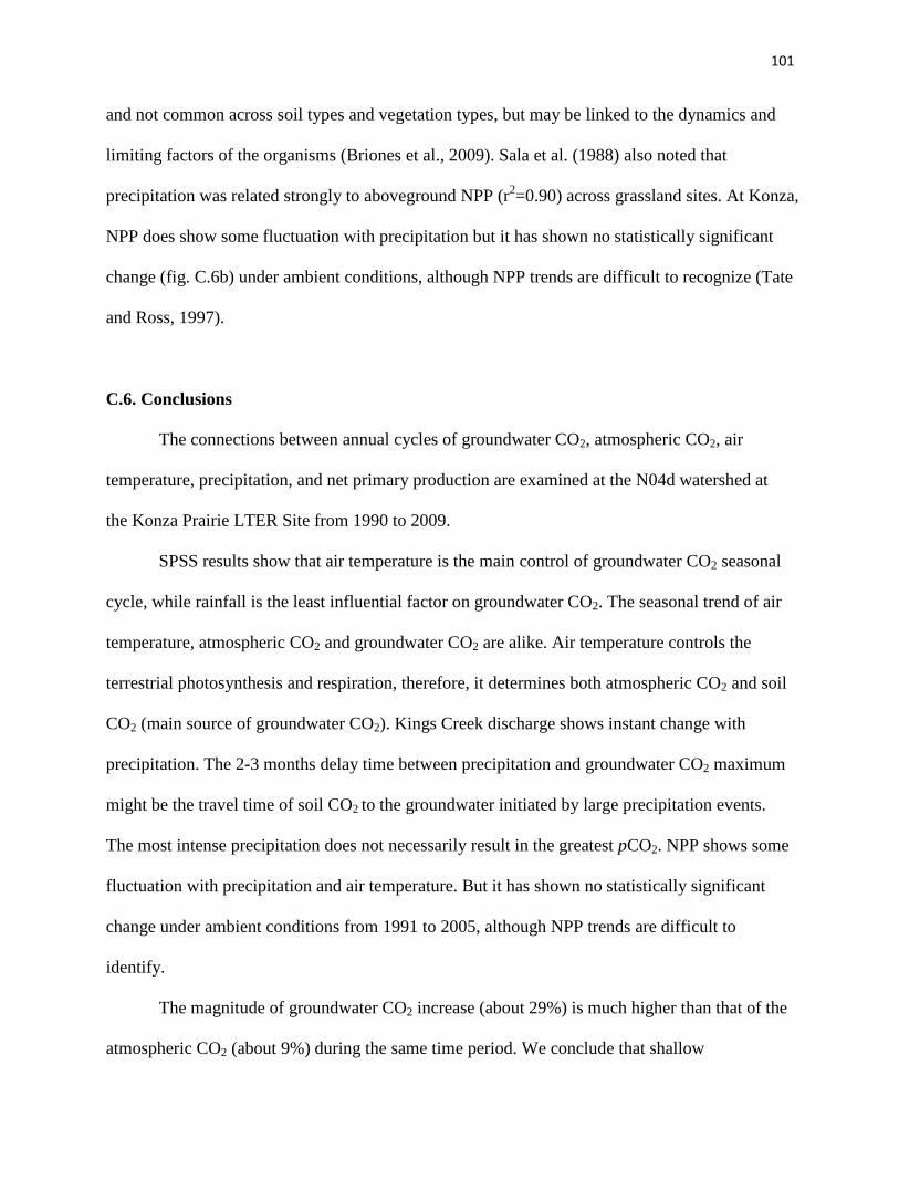
101
and not common across soil types and vegetation types, but may be linked to the dynamics and
limiting factors of the organisms (Briones et al., 2009). Sala et al. (1988) also noted that
precipitation was related strongly to aboveground NPP (r2=0.90) across grassland sites. At Konza,
NPP does show some fluctuation with precipitation but it has shown no statistically significant
change (fig. C.6b) under ambient conditions, although NPP trends are difficult to recognize (Tate
and Ross, 1997).
C.6. Conclusions
The connections between annual cycles of groundwater CO2, atmospheric CO2, air
temperature, precipitation, and net primary production are examined at the N04d watershed at
the Konza Prairie LTER Site from 1990 to 2009.
SPSS results show that air temperature is the main control of groundwater CO2 seasonal
cycle, while rainfall is the least influential factor on groundwater CO2. The seasonal trend of air
temperature, atmospheric CO2 and groundwater CO2 are alike. Air temperature controls the
terrestrial photosynthesis and respiration, therefore, it determines both atmospheric CO2 and soil
CO2 (main source of groundwater CO2). Kings Creek discharge shows instant change with
precipitation. The 2-3 months delay time between precipitation and groundwater CO2 maximum
might be the travel time of soil CO2 to the groundwater initiated by large precipitation events.
The most intense precipitation does not necessarily result in the greatest pCO2. NPP shows some
fluctuation with precipitation and air temperature. But it has shown no statistically significant
change under ambient conditions from 1991 to 2005, although NPP trends are difficult to
identify.
The magnitude of groundwater CO2 increase (about 29%) is much higher than that of the
atmospheric CO2 (about 9%) during the same time period. We conclude that shallow

102
groundwater is acting as a CO2 sink because CO2 build-up in the shallow aquifer is much faster
than the atmospheric CO2 growth.
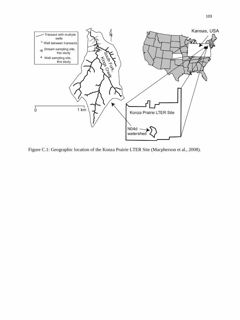
103
Figure C.1: Geographic location of the Konza Prairie LTER Site (Macpherson et al., 2008).
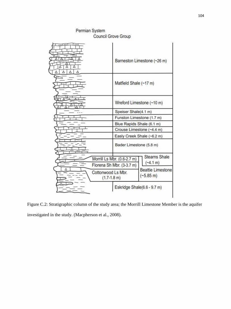
104
Figure C.2: Stratigraphic column of the study area; the Morrill Limestone Member is the aquifer
investigated in the study. (Macpherson et al., 2008).
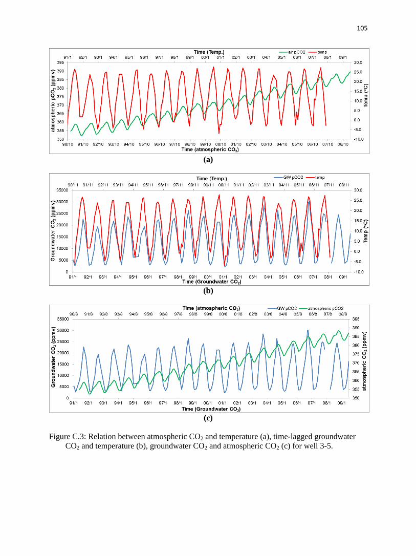
105
(a)
(b)
(c)
Figure C.3: Relation between atmospheric CO2 and temperature (a), time-lagged groundwater
CO2 and temperature (b), groundwater CO2 and atmospheric CO2 (c) for well 3-5.
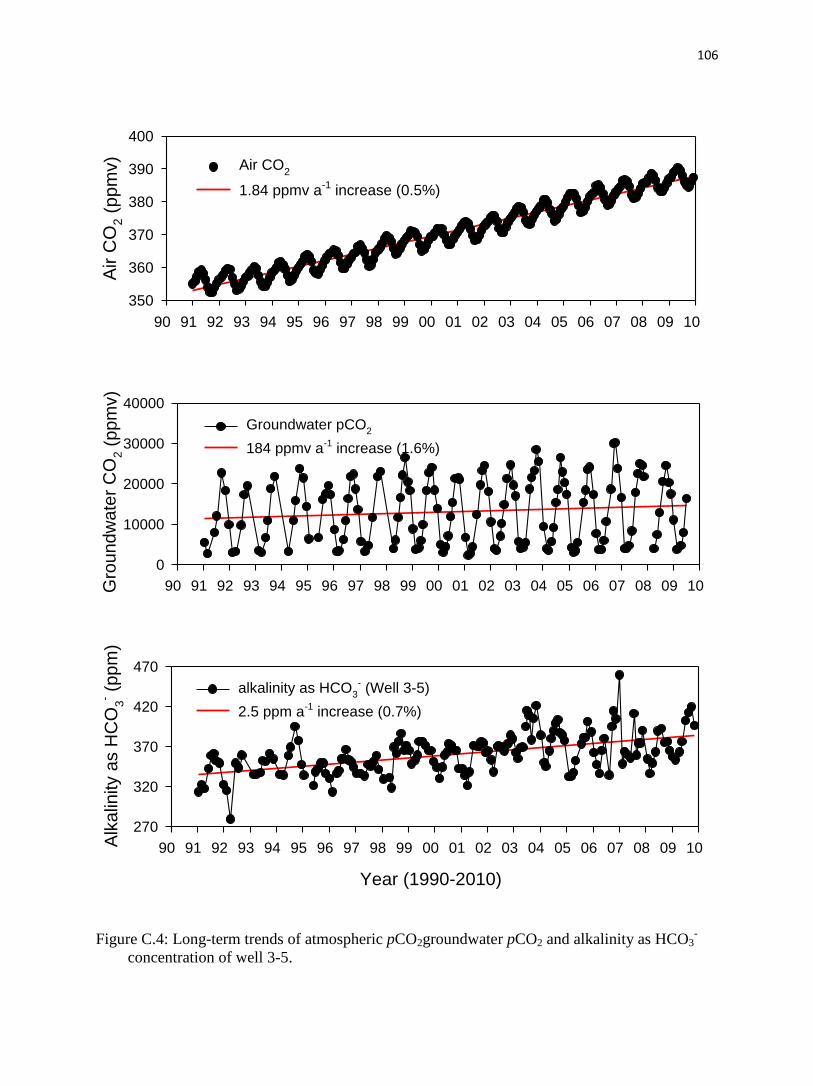
106
90 91 92 93 94 95 96 97 98 99 00 01 02 03 04 05 06 07 08 09 10
Air C
O2 (
pp
mv)
350
360
370
380
390
400
Air CO2
1.84 ppmv a-1 increase (0.5%)
90 91 92 93 94 95 96 97 98 99 00 01 02 03 04 05 06 07 08 09 10 Gro
und
wate
r C
O2 (
ppm
v)
0
10000
20000
30000
40000
Groundwater pCO2
184 ppmv a-1 increase (1.6%)
Year (1990-2010)
90 91 92 93 94 95 96 97 98 99 00 01 02 03 04 05 06 07 08 09 10 Alk
alin
ity a
s H
CO
3
- (ppm
)
270
320
370
420
470
alkalinity as HCO3
- (Well 3-5)
2.5 ppm a-1 increase (0.7%)
Figure C.4: Long-term trends of atmospheric pCO2groundwater pCO2 and alkalinity as HCO3-
concentration of well 3-5.
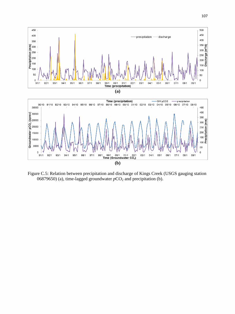
107
(a)
(b)
Figure C.5: Relation between precipitation and discharge of Kings Creek (USGS gauging station
06879650) (a), time-lagged groundwater pCO2 and precipitation (b).
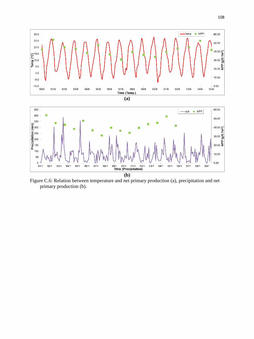
108
(a)
(b)
Figure C.6: Relation between temperature and net primary production (a), precipitation and net
primary production (b).
109
Appendix D. Geochemical speciation modeling results from PHREEQC
For Konza May sampling, pH, DO and temperature along with laboratory-determined
alkalinity, other anions, and cations were input in PHREEQC (Parkhurst and Appelo,1999) to
calculate CO2 partial pressure (pCO2) and the calcite saturation index (SIc) for each record.
For Maolan sampling, water temperature, pH, DO, estimated Ca2+
and HCO3-, with mean
monthly values of K+, Na
+, Mg
2+, Cl
– and SO4
2– (resolutions are 0.01 mg/L), were speciated
using PHREEQC to calculate pCO2 and the SIc for each data set.
For the Konza Prairie long-term data, the full chemical analysis and SIc of well 3-5 and
well 4-6 are input in PHREEQC to calculate the pH and the partial pressure of CO2.
110
References cited in all appendices
Amthor, J.S., 1995. Terrestrial higher-plant response to increasing atmospheric [CO2] in relation
to the global carbon cycle. Global Change Biology 1, 243-274.
Andresen, L.C., Michelsen, A., Ambus, P., Beier, C., 2010. Belowground heathland responses
after 2 years of combined warming, elevated CO2 and summer drought. Biogeochemistry
101, 27-42.
Bond-Lamberty, B., Thomson, A., 2010. Temperature-associated increases in the global soil
respiration record. Nature 464, 579–582.
Briones, M.J.I., Ostle, N.J., McNamara, N.P., Poskitt, J., 2009. Functional shifts of grassland soil
communities in response to soil warming. Soil Biol. Biochem. 41, 315–322.
Buchanan, D.L., Corcoran, B.J., 1959. Sealed tube combustions for the determination of
carbon-14 and total carbon. Anal. Chem. 31, 1635–1638
Buermann, W., Lintner, B.R., Koven, C.D., Angert, A., Pinzon, J.E., Tucker, C.J., Fung, I.Y.,
2007. The changing carbon cycle at Mauna Loa Observatory. PNAS Environ. Sci. 104,
4249–4254.
Dodds, W.K., Evans-White, M.A., Gerlanc, N.M., Gray, L., Gudder, D.A., Kemp, M.J., Lopez,
A.L., Stagliano, D., Strauss, E.A., Tank, J.L., Whiles, M.R., Wollheim, W.M., 2000.
Quantification of the nitrogen cycle in a prairie stream. Ecosystems 3, 574–589.
Freeman, C.C., 1998. The flora of Konza Prairie: a historical review and contemporary patterns.
In: Knapp, A.K., Briggs, J.M., Hartnett, D.C., Collins, S.L. (Eds.), Grassland Dynamics –
Long-Term Ecological Research in Tallgrass Prairie. Oxford University Press, New York,
69–80.
Gray, L.J., Macpherson, G.L., Koelliker, J.K., Dodds, W.K., 1998. Hydrology and aquatic
chemistry. In: Knapp, A.K., Briggs, J.M., Hartnett, D.C., Collins, S.L. (Eds.), Grassland
111
Dynamics – Long-Term Ecological Research in Tallgrass Prairie. Oxford University
Press, New York, 159–176.
Hayden, B., 1998. Regional climate and the distribution of tallgrass prairie. In: Knapp, A.K.,
Briggs, J.M., Hartnett, D.C., Collins, S.L. (Eds.), Grassland Dynamics –Long-Term
Ecological Research in Tallgrass Prairie. Oxford University Press, New York, 19–34.
Harmon, M.E., Ferrell, W.K., Franklin, J.F., 1990. Effects on carbon storage of conversion of
old-growth forests to young forests. Science 247, 699-702.
Hendry, M.J., Mendoza, C.A., Kirkland, R.A., Lawrence, J.R., 1999. Quantification of transient
CO2 production in a sandy unsaturated zone. Water Resour. Res. 35, 2189–2198.
Johnson, W.C., Willey, K.L, Macpherson, G.L., 2007. Carbon isotope variation in modern soils
of the tallgrass prairie: analogues for the interpretation of isotopic records derived from
paleosols. Quat. Int. 162, 3–20
Kissing, K. R., Macpherson, G. L., 2006. Short-term water-level fluctuations and long-term
water-level decline at the Konza Prairie—drought or vegetation?.Geol. Soc. Am. Absts.
Progs. 3835.
Liu, Z., Li, Q., Sun, H., Wang, J., 2007. Seasonal, diurnal and storm-scale hydrochemical
variations of typical epikarst spring in subtropical karst areas of SW China: soil CO2 and
dilution effects. J. Hydrol. 337, 207–223.
Macpherson, G. L.,1992. Ground-water chemistry under tallgrass prairie, central Kansas, USA.
In Proceedings of the 7th
International Symposium on Water–Rock Interaction, Park City,
Utah, USA(eds. Y. K. Kharak and A. S. Maest). A.A. Balkema, Brookfield, 809–812.
Macpherson, G. L., 1996. Hydrogeology of thin limestones–the Konza Prairie LTER Site. J.
Hydrol. 186, 191–228.
Macpherson G. L. (2004) Field vs. lab pH in remote wells, Konza Prairie LTER site, and
implications for limestone weathering. In Proceedings of the 11th International
112
Symposium on Water–Rock Interaction, Saratoga Springs, New York, USA(eds. R. B.
Wanty and R. R. Seal, II). A.A. Balkema, New York, 845–848.
Macpherson, G. L., Roberts J. A., Blair J. M., Townsend M. A., Fowle D. A., Beisner K. R.
2008. Increasing shallow groundwater CO2 and limestone weathering, Konza Prairie,
USA. Geochimica et Cosmochimica Acta, v. 72, i. 23, pp. 5581-5599.
Milly, P.C.D., Wetherald, T.R., Dunne, K.A., Delworth, T.L., 2002. Increasing risk of great
floods in a changing climate. Nature 415, 514 – 517.
Oviatt, C. G., 1998. Chapter 3 geomorphology of Konza Prairie. In Grassland Dynamics (eds. A.
K. Kn app, J. M. Briggs, D. C. Hartnett and S. L. Collins). Oxford Univ. Press, New
York, pp. 35–47.
Parkhurst, D., L., and Appelo, C., A., J., 1999. User’s guide to PHREEQC (Version 2)—a
computer program for speciation, batch-reaction, one-dimensional transport, and inverse
geochemical calculations.U.S. Geol. Surv. Wat.-Resour. Investigations Report 99-4259,
p. 312.
Pomes, M.L., 1995. A study of the aquatic humic substances and hydrogeology in a prairie
watershed, use of humic material as a tracer of recharge through soils. Ph.D. thesis, Univ.
Kansas
Ransom, M.D., Rice, C.W., Todd, T.C., Wehmueller, W.A., 1998. Soils and soil biota. In:
Knapp, A.K., Briggs, J.M., Hartnett, D.C., Collins, S.L. (Eds.), Grassland Dynamics –
Long-Term Ecological Research in Tallgrass Prairie. Oxford University Press, New
York, pp. 48–66.
Reiners, W.A., 1972. Structure and energetics of three Minnesota forests. Ecological
Monographs 42, 71-94.
113
Runyon, J., Waring, R.H., Goward, S.N., Welles, J.M., 1994. Environmental limits on net
primary production and light-use efficiency across the Oregon transect. Ecological
Applications 4, 226-237.
Sala, O.E., Parton, W.J., Joyce, L.A., Lauenroth, W.K., 1988. Primary production of the central
grassland region of the United States. Ecology 69, 40-45.
Schulte, P., Geldern, R., Freitag, H., Karim, A., 2011. Applications of stable water and carbon
isotopes in watershed research: Weathering, carbon cycling, and water balances.
Earth-Sci. Rev., 109, 20-31.
Singh, J.S., Lauenroth, W.K., Steinhorst, R.K., 1975. Review and assessment of various
techniques for estimating net aerial primary production in grasslands from harvest data.
Botanical Review 41, 181-232.
Tate, K. R., and Ross, D. J., 1997. Elevated CO2 and moisture effects on soil carbon storage and
cycling in temperature grasslands. Glob. Change Biol.3, 225–235.
Thomas, R.B., Lewis, J.D., and Strain, B.R., 1994. Effects of leaf nutrient status on
photosynthetic capacity in loblolly pine seedlings grown in elevated atmospheric CO2.
Tree Physiology 14, 947-960.
Towne, E.G., 2002. Vascular plants of Konza prairie biological station: an annotated checklist of
species in a Kansas tallgrass prairie. Sida 20, 269–294.
Tsypin, M., and Macpherson, G.L., 2012. The effect of precipitation events on inorganic carbon
in soil and shallow groundwater, Konza Prairie LTER Site, NE Kansas, USA. Applied
Geochemistry 27, 2356–2369.
Twiss, P.C., 1988. Beattie limestone (lower Permian) of eastern Kansas. In: Hayward, O.T.
(Ed.), G.S.A. Centennial Field Guide, vol. 4, South-Central Section of the Geological
Society of America. Geol. Soc. Am., 35–41.
114
Vinter, M. A. and I. C. Burke, 1997. Contingent effects of plant species on soils along a regional
moisture gradient in the Great Plains. Oecologia 110, 393-402.
Wehmueller, W.A., Campbell, H.V., Hamilton, V.L., Graber, S.P., 2005. Soil survey of Geary
County, Kansas. US Dept. of Agriculture, Natural Resources Conservation Service.
White, W. B., 1969. Conceptual models for carbonate aquifers. Ground Water 7, 15–21.
Zeller, D.E. (Ed.), 1968. The Stratigraphic Succession in Kansas. Kansas Geol. Survey Bull. 189.