INNOVATIVE SPARSE REPRESENTATION ALGORITHMS FOR ROBUST FACE

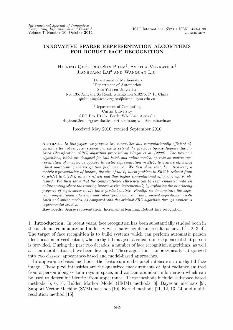
International Journal of InnovativeComputing, Information and Control ICIC International c⃝2011 ISSN 1349-4198Volume 7, Number 10, October 2011 pp. 5645–5667

INNOVATIVE SPARSE REPRESENTATION ALGORITHMSFOR ROBUST FACE RECOGNITION

Huining Qiu1, Duc-Son Pham2, Svetha Venkatesh2

Jianhuang Lai3 and Wanquan Liu2

1Department of Mathematics3Department of Automation

Sun Yat-sen UniversityNo. 135, Xingang Xi Road, Guangzhou 510275, P. R. China

[email protected]; [email protected]

2Department of ComputingCurtin University

GPO Box U1987, Perth, WA 6845, [email protected]; [email protected]; [email protected]

Received May 2010; revised September 2010

Abstract. In this paper, we propose two innovative and computationally efficient al-gorithms for robust face recognition, which extend the previous Sparse Representation-based Classification (SRC) algorithm proposed by Wright et al. (2009). The two newalgorithms, which are designed for both batch and online modes, operate on matrix rep-resentation of images, as opposed to vector representation in SRC, to achieve efficiencywhilst maintaining the recognition performance. We first show that, by introducing amatrix representation of images, the size of the ℓ1-norm problem in SRC is reduced fromO(whN) to O(rN), where r ≪ wh and thus higher computational efficiency can be ob-tained. We then show that the computational efficiency can be even enhanced with anonline setting where the training images arrive incrementally by exploiting the interlacingproperty of eigenvalues in the inner product matrix. Finally, we demonstrate the supe-rior computational efficiency and robust performance of the proposed algorithms in bothbatch and online modes, as compared with the original SRC algorithm through numerousexperimental studies.Keywords: Sparse representation, Incremental learning, Robust face recognition

1. Introduction. In recent years, face recognition has been substantially studied both inthe academic community and industry with many significant results achieved [1, 2, 3, 4].The target of face recognition is to build systems which can perform automatic personidentification or verification, when a digital image or a video frame sequence of that personis provided. During the past two decades, a number of face recognition algorithms, as wellas their modifications, have been developed. These algorithms can be typically categorizedinto two classes: appearance-based and model-based approaches.

In appearance-based methods, the features are the pixel intensities in a digital faceimage. These pixel intensities are the quantized measurements of light radiance emittedfrom a person along certain rays in space, and contain abundant information which canbe used to determine identity from appearance. These methods include: subspace-basedmethods [5, 6, 7], Hidden Markov Model (HMM) methods [8], Bayesian methods [9],Support Vector Machine (SVM) methods [10], Kernel methods [11, 12, 13, 14] and multi-resolution method [15].

5645

5646 H. QIU, D.-S. PHAM, S. VENKATESH, J. LAI AND W. LIU

For model-based approaches, general shape models of human faces are introduced,such as Elastic Bunch Graph Matching (EBGM) [16], Active Appearance Model (AAM)[17] and 3D Morphable Model method [18]. These methods employ general facial shapemodels as representations of faces, like face bunch graph, or model with landmark points,or model of 3D face shape and texture. The image pixels are treated as low level featureswhich need to be extracted into high level features before adapting to these models. Aface image of a person is assumed to be the output of the face model corresponding toinput parameters, and face recognition is transformed into a model matching problem.In the literature of face recognition, the appearance-based methods have been exten-

sively studied, among which only the subspace-based algorithms are reviewed here. Someof the subspace-based algorithms include: Eigenfaces and its variants [19, 20], Fisherfacesand its numerous modifications [21, 22], Laplacianfaces and its extensions [23, 24], ICA-based methods [25], NMF-based methods [26, 27], to name only a few. Most of thesetechniques depend on a representation of images in a vector space structure. Algorithmsthen adopt statistical techniques to analyze the distribution of the object image vectors,and find effective representations in a transformed vector space (feature space) accordingto various criteria. Once a test image is captured, the similarity between the test imageand the prototype training sets is then calculated in the feature space. Face recognitionin this category is in fact a learning process with optimization techniques.So far, face recognition in controlled environments has reached its maturity with high

performance. However, face recognition in less controlled or uncontrolled environmentsstill requires further study in order to be usable in practice. Recent standardized vendorface technology tests revealed that there are still major challenges in practical face recogni-tion applications [28, 29, 30, 31]. The main challenges are the potential large intra-subjectvariations in human face image appearance due to 3D head pose changes, illuminationvariants (including indoor/outdoor conditions), facial expressions, occlusions with otherobjects or accessories (e.g., sunglasses, scarfs), facial hair and aging. As these difficultiesexist in face recognition, more robust face recognition algorithms are still needed.Recently, Wright et al. [32] have developed a new face recognition framework for the

robust face recognition problem. Their work is based on a newly developed compressedsensing theory, and has shown its robust performance compared with traditional facerecognition techniques. Compressed sensing is a technique first developed in signal pro-cessing community for reconstructing a sparse signal by utilizing the prior knowledge ofits sparsity structure [33, 34]. Classical signal reconstruction method is to minimize theℓ2 norm, which is equivalent to minimizing the amount of energy in the system. The com-pressed sensing theory resolves to minimize the ℓ0 norm, which is equivalently relaxed tominimizing the ℓ1 norm under certain conditions. It yields attractive solutions which showtheir robust property against noises in many problems. Due to its mathematics founda-tion and effective framework, compressed sensing has already drawn immense attentionin areas of mathematics, optimization, information theory, statistical signal processing,high-dimensional data analysis [35, 36, 37]. A survey about compressed sensing and itsbroad applications can be found in [38].The idea of compressed sensing is adopted by Wright et al. in their new algorithm

for face recognition, namely Sparse Representation-based Classification (SRC) algorithm.This algorithm is robust in a sense that the sparse representation is less sensitive tooutliers in the face images such as occlusion or random pixel corruptions. However, themajor disadvantage of the SRC algorithm is its very expensive computational cost, whichlimits its current applicability. Due to its vector representation, the SRC needs to solvean ℓ1-regularized optimization problem whose size is the total number of pixels of theimages, which can be extremely large when high resolution images are used.

INNOVATIVE SR ALGORITHMS FOR ROBUST FACE RECOGNITION 5647

To overcome the computational issue, two approaches can be considered. First, di-mensionality reduction can be performed on the input images and then extracted featurevectors can be used instead of original pixel features. However, this approach might poten-tially lose beneficial information in the original images. Second, equivalent reformulationof the problem can be pursued to find the solution faster, and the optimization problemcan be solved with proper acceleration technique. In this paper, we follow the second al-ternative and aim to reduce computational complexity of the SRC algorithm by workingdirectly on 2D representation of images. Our method is accomplished by reformulatingthe 2D images sparse representation problem, and then solving it through the existingℓ1 optimization techniques. For convenience, hereinafter, we name the original SRC al-gorithm as 1D-SRC, and our new algorithm as 2D-SRC. Further, we consider applyingthe 2D-SRC algorithm in an incremental learning context, and propose an incremental2D-SRC learning procedure which has proved to be more efficient.

This paper is organized as follows: in Section 2, we review the SRC algorithm andpropose our 2D extension algorithm and the incremental computing procedure, followed bythe complexity analysis; then, in Section 3, we compare the performance of 1D-SRC with2D-SRC and the incremental algorithms on some benchmark datasets, and reveal thatthe proposed algorithms can speed up without decreasing the recognition performance;finally, we conclude the paper in Section 4.

2. SRC Algorithms and Their Computational Complexity. We first present theoriginal 1D-SRC algorithm and analyze its high computational cost problem, then wepropose an equivalent formulation and induce a 2D-SRC algorithm which can be solvedmuch faster. After that, we further extend the 2D-SRC algorithm into the incrementallearning context. At last, we discuss the computational complexity of the three algorithms.

2.1. The SRC algorithm. In this subsection, we briefly review the sparse representationface model and the SRC algorithm.

In face recognition research, it is generally conceived that there exists a face subspacewhich is formed by one person’s face images under different variations (e.g., pose, illumi-nation, expression). As a result, linear models can be used to approximate these “facesubspaces”. The recently proposed sparse representation-based face model is developedbased on this hypothesis, and it uses all known training sample images to span a facesubspace. For a test face image whose class label is unknown, one tries to reconstruct thetest image sparsely from the training samples.

The motivation of this model is that if given sufficient training samples of one person,then any new (test) sample for this person will approximately lie in the linear span of thetraining samples associated with this person. To be more precise, let us say, a databaseconsists of k classes denoted as:

A = {A1,1, . . . ,A1,n1 , . . . ,Ak,1, . . . ,Ak,nk}

where Ai,l is the l-th image belonging to class i, ni is number of samples for class i,i = 1, . . . , k. By stacking pixels of each image Ai,l into a column vector vi,l, one can buildup a matrix A to represent the training samples

A = [v1,1, . . . ,v1,n1 , . . . ,vk,1, . . . ,vk,nk] ∈ RL×N (1)

where L = hw is the number of pixels for a h× w image, N = n1 + . . . + nk is the totalnumber of samples for all classes.

For a new test image y, we then can represent it using linear combination of samplesfrom the database

y = Ax0. (2)


Most ideally, if y is from person i, then based on the assumption that person i’s facesubspace is sufficient to represent itself, so the coefficients x0 should have a form of

x0 = [0, . . . , 0, αi,1, αi,2, . . . , αi,ni, 0 . . . , 0] (3)

in other words, the solution x0 in linear Equation (2) should only have non-zero valuesat positions corresponding to the same person as the test image, therefore, it should bevery sparse. Thus, one can use “sparsity” as a heuristic principle for solving the linearEquation (2), even though not knowing the true identity of the test image. For thispurpose, one can set up an objective to measure the “sparsity” of the coefficients x. Fromthe compressed sensing theory one knows that a restriction of ℓ1-norm has an effect ofproducing sparse solutions. So, this leads to the following least ℓ1-norm problems:

(ℓ1) :x1 = arg min

x∥x∥1

s.t. Ax = y.(4)

and

(ℓs1) :x1 = arg min

x∥x∥1

s.t. ∥Ax− y∥2 ≤ ϵ.(5)

The above two models are both used in the SRC algorithm, and they are differentbecause (4) is a noise-free model and (5) is a model in the existence of noises. However,they can be solved using the same optimization technique.Now the SRC algorithm can be summarized as in Algorithm 1:

Algorithm 1 Sparse Representation-based Classification (1D-SRC byWright et al. [32])1: Input: a matrix of training samples for k classes

A = [v1,1, . . . ,v1,n1 , . . . ,vk,1, . . . ,vk,nk] ∈ R(wh)×N

(each column of A is a vectorization of training sample image Ai,il); the class labelsclass(p), p = 1, . . . , k; the corresponding class labels label(i) of each training samplevector A(:, i); a test sample y ∈ R(wh)×1; an optional error tolerance parameter ϵ > 0.

2: Normalize the columns of A to have unit ℓ2-norm.3: Solve the ℓ1-norm minimization problem

x = arg minx∥x∥1 s.t. Ax = y.

or alternatively solve the ℓ1-norm minimization problem

x = arg minx∥x∥1 s.t. ∥Ax− y∥2 ≤ ϵ.

4: Compute the per-class residuals

rp (y) = ∥y − Aδp (x) ∥2 for p = 1, . . . , k.

where δp (x), for p = 1, . . . , k is a new vector for the p-th class whose entries aredefined as:

for i = 1, . . . , N, δ(i)p (x) =

{xi, if label(i) is class(p)0, otherwise.

5: Output: identity(y) = class(p∗), p∗ = arg minp

rp (y) .

Based on the experimental results reported in [32], the SRC algorithm demonstratesrobust performance for face datasets with noises and occlusions, and can attain highrecognition rates.


2.2. The 2D-SRC algorithm. In this section, we are concerned with the computationalcost of the SRC algorithm. From Algorithm 1, we can find that the most time consumingstep of the SRC algorithm is Step 3, which needs to solve the ℓ1-norm minimizationproblem (4) or (5). Further, the problem size of the ℓ1-norm minimization is determinedby the size of matrix A. More precisely, it is proportionally increasing to size(A) = L×N ,where L is the image dimensionality, i.e., the total pixel counts L = wh, and N is thetraining sample size. So, if either the image dimensionality or the training sample sizeis very large, then the computation of solving the ℓ1-norm minimization problem willbecome very slow, or even failed. For example, a typical face database usually containsimages whose facial area can easily take up 90× 90 = 8100 pixels, which is an extremelyhigh dimensionality and can cause great computational costs. In this case, the SRCalgorithm does not work well because it cannot find the least ℓ1-norm solution effectively.To overcome this problem, the authors in [32] proposed to downsize the original imagesinto smaller images which can make the computation possible, and all their computationsthere are executed upon these smaller images. Although such downsampling of the imagescan reduce the problem size and enable to compute attractable solutions, it also leads toloss of discriminant information which are important for classification. Though thereexist other dimensionality reduction methods which can reduce the problem size of ℓ1-norm minimization, it is better to preserve the discriminant information by using theoriginal images directly. Next, we devote to developing a 2D-SRC algorithm for thispurpose.

We first analyze the 1D-SRC model before investigation of a 2D-SRC model. Accordingto Fuchs [39, 40] and Boyd [41], the linear programming problem (4) and the quadraticprogramming problem (5) can be equivalently transformed into the following ℓ1-normregularization problem

x1 = arg minx

λ∥x∥1 + ∥Ax− y∥22 for some λ. (6)

This transformation is equivalent provided the parameter λ is adequately chosen. Thusthis transformation can unify problems (4) and (5) with an aim of simplifying the pro-cess of the SRC algorithm. We start inducing a 2D-SRC model on basis of this newtransformation.

We notice that in (6) the matrix A is formed by stacking each h × w image Ai into along vector vi and then putting it to be a column of the matrix, thus A is a large matrixsince its row number is equal to the dimensionality of images. In order to overcome thedimensionality curse problem, we represent each image as a matrix instead of a vector, toderive a 2D sparse representation model that is similar to (6). For convenience, hereafterwe use the bold symbols Ai and A to denote the matrices of the training images andthe test image respectively. For a test image A, we suppose it can be represented by thewhole training images with a linear combination as follows:

A =N∑i=1

xiAi (7)

where xi (i = 1, . . . , N) are the coefficients need to be determined. Further, we canformulate the following ℓ1-norm regularization problem under the sparse representationassumption

x1 = arg minx

λ∥x∥1 +∥∥∥∥A− N∑

i=1

xiAi

∥∥∥∥2

F

(8)


where A is an h×w image matrix whose label is to be determined, Ai (i = 1, . . . , N) is aset of training image matrices whose class labels are already known, ∥·∥F is the Frobenius

matrix norm, x = [x1, . . . , xN ]T is the sparse coefficients, and λ is a regularization pa-

rameter that needs to be adequately chosen. Denote Kh×w the vector space containing allreal matrices with h rows and w columns, we can introduce the Frobenius inner productas follows:

⟨A,B⟩F =∑i

∑j

AijBij. (9)

The Frobenius inner product is related to the Frobenius matrix norm by the followingequation

⟨A,A⟩F =∑i

∑j

A2ij = ∥A∥2F . (10)

Accordingly, we can rewrite the reconstruction error term in 2D-SRC model (8) as:

∥A−∑i

xiAi∥2F (11)

=

⟨A−

∑i

xiAi,A−∑i

xiAi

⟩F

(12)

=∑i

∑j

xixj ⟨Ai,Aj⟩F − 2∑i

xi ⟨Ai,A⟩F + ∥A∥2F

= xTQx− 2bTx+ c (13)

where

Q =

⟨A1,A1⟩F . . . ⟨A1,AN⟩F...

. . ....

⟨AN ,A1⟩F · · · ⟨AN ,AN⟩F

∈ ℜN×N , (14)

b =

⟨A1,A⟩F⟨A2,A⟩F

...⟨AN ,A⟩F

∈ ℜN×1, (15)

c = ∥A∥2F . (16)

As we can see from (13) that the 2D-SRC model objective function is actually a qua-dratic form, and the problem size is only proportional to the number of input samplesN . As Q is symmetric and positive semidefinite, we can always find a matrix with fullcolumn rank P = [p1, . . . ,pr] such that

Q = PTP. (17)

Then we can rewrite the quadratic form (13) as:

(13) = (Px)T (Px)− 2bTx+ c (18)

if further we can find a vector z such that

PTz = b (19)


then (18) becomes

(18) = (Px)T (Px)− 2(PTz

)Tx+ c (20)

= (Px)T (Px)− 2zT (Px) + zTz− zTz+ c (21)

= ∥Px− z∥2 − zTz+ c. (22)

And finally, we are able to transform the original 2D-SRC problem equivalently to

x1 = arg minx

λ∥x∥1 + ∥A−∑i

xiAi∥2F for some λ, (23)

⇔ x1 = arg minx

λ∥x∥1 +(∥Px− z∥2 − zTz+ c

)for some λ, (24)

⇔ x1 = arg minx

λ∥x∥1 + ∥Px− z∥2 for some λ. (25)

Thus, the 2D-SRC model (8) can lead to a smaller size ℓ1-minimization problem (25).The problem size now becomes size(P) = r ×N , and is smaller than the problem size ofthe 1D-SRC model, which is L × N . We can prove r ≤ min(L,N) (see Lemma 1 in theAppendix).

The only question left is how to find feasible P and z that satisfy (17) and (19). Inorder to find a P , let the compact Singular Value Decomposition (SVD) of Q be

Q = USUT =(US1/2

) (US1/2

)T(26)

where S is a nonsingular diagonal matrix and U is a orthnormal matrix with full columnrank. By simply letting

P =(US1/2

)T(27)

one can obtain a desirable solution for P . Further, since the columns of U are orthogonal,one can easily solve PTz = b by

PTz = b (28)

⇒ PPTz = Pb (29)

⇒(US1/2

)T (US1/2

)z = Pb (30)

⇒ z = S−1Pb. (31)

Once P and z are obtained as above, the 2D-SRC model is established. This model canstill be solved by the optimization technique used in [32], but the size of the problem ismuch smaller.

Based on the original 1D-SRC algorithm, we can now describe the 2D-SRC algorithmas Algorithm 2.

2.3. The incremental 2D-SRC algorithm. In this section, we further extend the pro-posed 2D-SRC algorithm to an incremental learning context. Consider scenarios whentraining data samples are coming incrementally, it is beneficial to reuse previous compu-tational results rather than to compute each time from scratch. For the 2D-SRC problem,when the training image samples are coming incrementally, we devote to derive an incre-mental learning algorithm for classifier design. In this paper, we only consider adding oneimage into the training image set each time for simplicity.

Assume that the current training images set is An = {A1,A2, . . . ,An}, and a newimage An+1 is labeled and added to form An+1 = An ∪ {An+1}. For this new images setAn+1, the 2D-SRC algorithm can be readily applied. However, this implies that we needto do SVD on the new inner product matrix Qn+1 =

[⟨Ai,Aj⟩F

]i,j=1,...,n+1

. In this way,

we have dropped all our previous computed results, especially the SVD results on the


previous inner product matrix Qn =[⟨Ai,Aj⟩F

]i,j=1,...,n

. As we can observe that in the

2D-SRC algorithm, computing SVD of the Frobenius inner product matrix Q is a criticalstep. If we can reduce the cost of each SVD computation, then we can further improvethe 2D-SRC efficiency with incremental learning.

Algorithm 2 2D Sparse Representation-based Classification (2D-SRC)1: Input: a set of training sample images for k classes

{A1,1, . . . ,A1,n1 , . . . ,Ak,1, . . . ,Ak,nk} ⊂ ℜh×w

the corresponding class labels label(i) of each training sample image Ai, a test sampleA ∈ ℜh×w and a regularization parameter λ > 0.

2: Compute the Frobenius inner product matrix Q and vector b by (15).3: Apply SVD on Q to find the matrix P and vector z by (27) and (28).4: Solve the reduced ℓ1-minimization (1D-SRC) problem

x1 = arg minx

λ∥x∥1 + ∥Px− z∥22 for some λ. (32)

5: Compute the per-class residuals

rp (A) = ∥A−∑i

δ(i)p (x)Ai∥F for p = 1, . . . , k. (33)

where δp (x) , for p = 1, . . . , k is a vector for the p-th class whose entries are defined as:

for i = 1, . . . , N, δ(i)p (x) =

{xi, if label(i) is class(p)0, otherwise.

(34)

6: Output: identity(y) = class(p∗), p∗ = arg minp

rp (y).

First, we notice that for any n, Qn is an inner product matrix, so it is symmetric andpositive semidefinite. Therefore, computing the SVD of Qn is equivalent to computingthe Eigenvalue Decomposition (EVD) of Qn. What’s more favorable, all eigenvalues ofQn are non-negative (see Lemma 2 in Appendix). Consequently, we can focus on how tocompute the EVD of Qn+1 from the EVD of Qn. Mathematically, the problem can bestated as if given the EVD

Qn = UnΛnUTn (35)

and when a new sample An+1 is added, how can we compute the EVD

Qn+1 ≡[Qn bbT c

]= Un+1Λn+1U

Tn+1 (36)

efficiently, where b = [b1, b2, . . . , bn]T , bi = ⟨Ai,An+1⟩F (i = 1, . . . , n) and c =

⟨An+1,

An+1

⟩Fare the incremental inner products formed with the new sample.

This is actually a mathematical problem, and the following theorem provides us therelation between the eigenvalues and eigenvectors of Qn, Qn+1.

Theorem 2.1. (An Interlacing property of Eigenvalues [42]) Assume that the eigenvaluedecomposition (EVD) of Qn+1 is given by

Qn+1 ≡[Qn bbT c

]=

[UnΛnU

Tn b

bT c

]=

[Un 00 1

]Rn+1

[UT

n 00 1

](37)


where

Rn+1 ≡[

Λn UTnb

bTUn c

]≡

λ1 z1

. . ....

λn znz1 · · · zn c

(38)

has the property that its eigenvalues are exactly n+1 roots of the following equation w.r.t.variable d

z21d− λ1

+ · · ·+ z2nd− λn

= d− c. (39)

Moreover, if we let λ1 < λ2 < · · · < λn be sorted, and d1 < d2 · · · < dn < dn+1 be alln+ 1 sorted roots of (39), then the following interlacing relation holds

d1 < λ1 < d2 < λ2 < · · · < dn < λn < dn+1, (40)

and the eigenvector vi corresponding to its eigenvalue di can be obtained by solving theeigen-equation directly, which gives

vi =1Ti

[z1

di−λ1, · · · , zn

di−λn, 1], for i = 1, . . . , n+ 1 (41)

(Ti is a factor normalizing vi to be unit norm).

Finally, we have the EVDs

Vn+1 = [v1, . . . ,vn+1], Dn+1 = diag ([d1, . . . , dn+1]) (42)

Rn+1 = Vn+1Dn+1VTn+1 (43)

Un+1 =

([Un 00 1

]Vn+1

), Λn+1 = Dn+1 (44)

Qn+1 = Un+1Λn+1UTn+1. (45)

This gives the SVD of Qn+1.

In the above theorem, without losing generality we can assume all eigenvalues aredistinct and all zi = 0, and we leave intensive discussion about repeated eigenvalues orany zi = 0 for Lemma 3 in the Appendix. The properties of the matrix Rn+1 in Theorem2.1 are well studied in mathematics community [43, 44, 45, 46]. Based on the result inTheorem 2.1, we can design a binary search algorithm to find all n+1 eigenvalues of Qn+1

from (34) which is presented in Algorithm 3. Then we can compute the correspondingeigenvectors through (41)-(44). This makes the incrementally computing of the SVDpossible. Eventually, we can summarize the incremental learning procedure for the 2D-SRC algorithm in Algorithm 4.

Algorithm 3 Binary search for roots of Equation (39)1: Input: the current n eigenvalues λ1,. . . , λn, the values z1,. . . , zi and c, M = norm(Qn),convergent tolerance ϵ > 0.

2: For i = 1, . . . , n+ 1, binary search di in interval [λi−1, λi] (let λ0 = −M , λn+1 = M):let low = λi−1, high = λi

dodi = (λi−1 + λi);fval = (di − c)−

∑ni=1 z

2i / (di − λi);

if fval > 0 then low = mid, else high = di;while fabs(high− low) > ϵ

3: Output: the new n+ 1 eigenvalues d1, . . . , dn+1.


Algorithm 4 Incremental procedure for 2D-SRC1: Assume that we have established a 2D-SRC model (by Algorithm 2) for n trainingimages, and now a new (n+ 1)-th training image is added.

2: Given current training sample image set {A1, . . . ,An} ⊂ ℜh×w with their label set,a saved copy of SVD decomposition on current Frobenius inner product matrix Qn

= UnΣnUTn , a new labeled training sample image An+1 ∈ ℜh×w.

3: Compute the new formed Frobenius inner product matrix entries b = [b1, b2, . . . , bn]where bi = ⟨Ai,An+1⟩F (i = 1, . . . , n) and c = ⟨An+1,An+1⟩F .

4: Compute all eigenvalues Σn+1 = diag (d1, . . . , dn+1) by Algorithm 3.5: Compute all eigenvectors Un+1 by (41) – (44).6: This establishes a 2D-SRC model (Algorithm 2) with training image set{A1, . . . ,An,An+1}.

7: n← n+ 1, and turn to Step 2.

2.4. Complexity analysis. One can see from the Algorithm 2 that the complexity ofestablishing a 2D-SRC model consists of two parts, the transformation step for findingparameters P and z and then solving the reduced ℓ1-minimization problem. In fact, themain computational cost in recognition is in the optimization process for solving the ℓ1-minimization problem. One can observe that problem size of the ℓ1-minimization problemin 1D-SRC is L × N and the one for the 2D-SRC is r × N . In most of applications, wehave L ≫ N and r < N , and this indicates that the 2D-SRC algorithm can speed upsignificantly.It is noted importantly that our analysis is based on an assumption that the smaller

the input size of ℓ1-norm solver, the faster it runs. Under this assumption, we can reducethe computational complexity from O(LN) to O(rN). Our experimental shows that onaverage the 2D-SRC algorithm is 2 ∼ 3 times faster than 1D-SRC, more details can beseen in our experimental results.As for the incremental SVD based version, its complexity also consists of two parts: let

n = size(Qn), then the binary searching steps for eigenvalues are at most C × n loops,where C is the maximum possible searching steps, and each loop contains O(n) float-pointoperations (flops); and the eigenvector computing step takes up O(n2) flops on computingall eigenvectors and it also needs an extra O(n2+δ) step for matrix-to-matrix multiplication(herein 0 ≤ δ ≤ 1 has not been well determined in computational complexity theory, buta δ ≈ 0.807 . . . algorithm has been presented in [47]; however, a naive implementation ofmultiplying two matrices will take n3 operations for δ = 1). Thus, totally it takes O(n2+δ)flops and can be more efficient than an independent SVD which generally needs O(n3)flops. We summarize the complexity comparisons in Table 1.

Table 1. Complexity of algorithms

SVD flops ℓ1-norm problem size1D-SRC – O(LN)2D-SRC O(N3) O(rN)

2D-SRC-incremental O(N2+δ)∗ O(rN)∗ here 0 ≤ δ ≤ 1 is still not determined in theory.

3. Experiments. To evaluate the efficiency of the proposed algorithms in this paper,we compare their computational costs and recognition rates with the 1D-SRC algorithmon several face recognition tasks. By using several benchmark face databases, we showthat the proposed two algorithms (2D-SRC and 2D-SRC-incremental) are faster than


the 1D-SRC algorithm, and recognition accuracy is maintained. Next, we present ourexperimental results in detail.

3.1. Datasets and configurations. We have performed experiments on three face data-bases: ORL [48], Yale B plus Extended [49, 50] and AR face database [51]. For eachdatabase, alignments (e.g., fixing positions for the two eyes, cropping) are performed.

For the ORL face database, it contains 40 individuals, each with 10 face images, sototally 400 face images are available; the original image size of the database is 92× 112,and we have cropped it into the size of 90× 90.

For the Yale B plus Extended face database, it contains 38 individuals, each with manyvariants of poses and illuminations, but in our experiments we only adopted these imageswith pose of frontal view (corresponding to those with filenames as ‘∗ P00∗’) and allilluminations in subset 1 and 2. We crop and resize them into 90× 90.

For the AR face database, we choose 120 individuals, each with 26 images available.We also crop and resize them into 90× 90.

An important advantage claimed for 1D-SRC model is its robust performance, so wedesign our experiments containing two parts: one part uses image datasets without cor-ruptions both for training and testing, the other part uses corrupted image datasets fortesting but not in training.

Although many ℓ1-optimization solvers are publicly available (e.g., [52, 53, 54]), ℓ1-magic [52] is chosen in [32]. More than that, in our experiments we also choose anotherℓ1-optimization solver l1 ls to solve the ℓ1-norm minimization problem. The purpose is tomake broad comparisons and investigate the performance in diversity when the proposedalgorithms are collaborating with different ℓ1-optimization solvers.

All the results are obtained using MATLAB on a machine with Intel(R) Xeon(R) CPU2.33GHz, 16GB of RAM, Windows Server 2003 Standard x64 Edition.

3.2. 1D-SRC vs. 2D-SRC accuracy and speed. In this part, we compare two algo-rithms: the original 1D-SRC algorithm and the proposed 2D-SRC algorithm. We focuson two performance: the recognition accuracy R and the average computational time T ,and they are defined as

R =nc

n, (46)

T =

∑ni=1 tin

(47)

where n is the total number of testing samples, nc is the number of correctly recognizedtesting samples, ti is the computational time used for recognizing the ith test sample.

The experiments are performed as follows: given a database, we split it using a half-halftraining:testing ratio (i.e., 50% : 50%), and for each split, we choose 5 random repeats ofthe training/testing set and record the performance of these two algorithms, then averagethe 5 rounds performance as a final performance. To test the performance of 1D-SRCand 2D-SRC under different image sizes, we also repeat resizing the same split sets withvarying sizes, and we have chosen the image size sequence as 20×20, 30×30, . . . , 80×80.

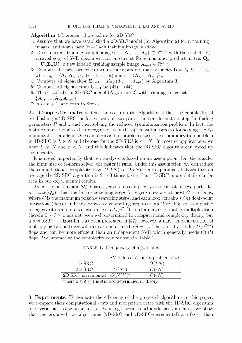
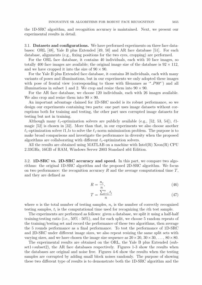
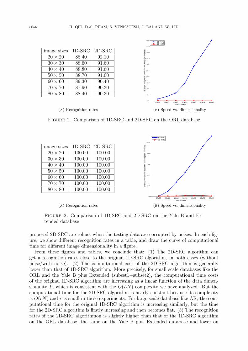
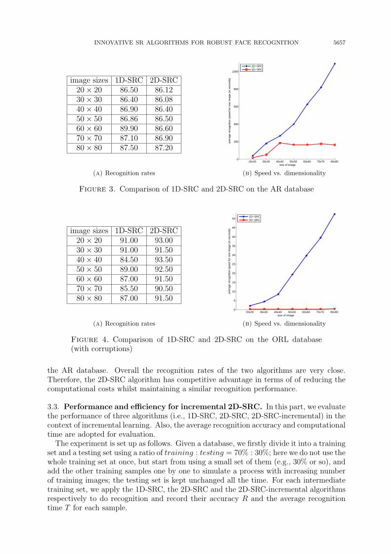
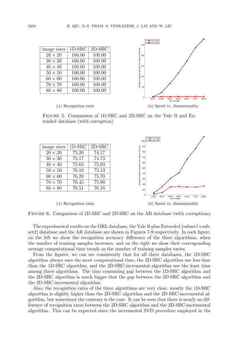
The experimental results are obtained on the ORL, the Yale B plus Extended (sub-set1+subset2), the AR face databases respectively. Figures 1-3 show the results whenthe databases are original and noise free. Figures 4-6 show the results when the testingsamples are corrupted by adding small block noises randomly. The purpose of showingthese two different type of results is to demonstrate both the 1D-SRC algorithm and the


image sizes 1D-SRC 2D-SRC20× 20 88.40 92.1030× 30 88.60 91.6040× 40 88.80 91.6050× 50 88.70 91.0060× 60 89.30 90.4070× 70 87.90 90.3080× 80 88.40 90.30

(a) Recognition rates

20x20 30x30 40x40 50x50 60x60 70x70 80x80 0

5

10

15

20

25

30

35

40

45

50

size of image

aver

age

reco

gniti

on s

peed

for

one

imag

e (in

sec

onds

)

1D−SRC2D−SRC

(b) Speed vs. dimensionality

Figure 1. Comparison of 1D-SRC and 2D-SRC on the ORL database



20x20 30x30 40x40 50x50 60x60 70x70 80x80 0

50

100

150

200

250

size of image

aver

age

reco

gniti

on s

peed

for

one

imag

e (in

sec

onds

)

1D−SRC2D−SRC


Figure 2. Comparison of 1D-SRC and 2D-SRC on the Yale B and Ex-tended database

proposed 2D-SRC are robust when the testing data are corrupted by noises. In each fig-ure, we show different recognition rates in a table, and draw the curve of computationaltime for different image dimensionality in a figure.From these figures and tables, we conclude that: (1) The 2D-SRC algorithm can

get a recognition rates close to the original 1D-SRC algorithm, in both cases (withoutnoise/with noise). (2) The computational cost of the 2D-SRC algorithm is generallylower than that of 1D-SRC algorithm. More precisely, for small scale databases like theORL and the Yale B plus Extended (subset1+subset2), the computational time costsof the original 1D-SRC algorithm are increasing as a linear function of the data dimen-sionality L, which is consistent with the O(LN) complexity we have analyzed. But thecomputational time for the 2D-SRC algorithm is nearly constant because its complexityis O(rN) and r is small in these experiments. For large-scale database like AR, the com-putational time for the original 1D-SRC algorithm is increasing similarly, but the timefor the 2D-SRC algorithm is firstly increasing and then becomes flat. (3) The recognitionrates of the 2D-SRC algorithmon is slightly higher than that of the 1D-SRC algorithmon the ORL database, the same on the Yale B plus Extended database and lower on




20x20 30x30 40x40 50x50 60x60 70x70 80x80 0

200

400

600

800

1000

size of image

aver

age

reco

gniti

on s

peed

for

one

imag

e (in

sec

onds

)

1D−SRC2D−SRC


Figure 3. Comparison of 1D-SRC and 2D-SRC on the AR database



20x20 30x30 40x40 50x50 60x60 70x70 80x80 0

5

10

15

20

25

30

35

40

45

50

size of image

aver

age

reco

gniti

on s

peed

for

one

imag

e (in

sec

onds

)

1D−SRC2D−SRC


Figure 4. Comparison of 1D-SRC and 2D-SRC on the ORL database(with corruptions)

the AR database. Overall the recognition rates of the two algorithms are very close.Therefore, the 2D-SRC algorithm has competitive advantage in terms of of reducing thecomputational costs whilst maintaining a similar recognition performance.

3.3. Performance and efficiency for incremental 2D-SRC. In this part, we evaluatethe performance of three algorithms (i.e., 1D-SRC, 2D-SRC, 2D-SRC-incremental) in thecontext of incremental learning. Also, the average recognition accuracy and computationaltime are adopted for evaluation.

The experiment is set up as follows. Given a database, we firstly divide it into a trainingset and a testing set using a ratio of training : testing = 70% : 30%; here we do not use thewhole training set at once, but start from using a small set of them (e.g., 30% or so), andadd the other training samples one by one to simulate a process with increasing numberof training images; the testing set is kept unchanged all the time. For each intermediatetraining set, we apply the 1D-SRC, the 2D-SRC and the 2D-SRC-incremental algorithmsrespectively to do recognition and record their accuracy R and the average recognitiontime T for each sample.




20x20 30x30 40x40 50x50 60x60 70x70 80x80 0

50

100

150

200

250

size of image

aver

age

reco

gniti

on s

peed

for

one

imag

e (in

sec

onds

)

1D−SRC2D−SRC


Figure 5. Comparison of 1D-SRC and 2D-SRC on the Yale B and Ex-tended database (with corruption)



20x20 30x30 40x40 50x50 60x60 70x70 80x80 0

100

200

300

400

500

600

700

800

900

1000

size of image

aver

age

reco

gniti

on s

peed

for

one

imag

e (in

sec

onds

)

1D−SRC2D−SRC


Figure 6. Comparison of 1D-SRC and 2D-SRC on the AR database (with corruptions)

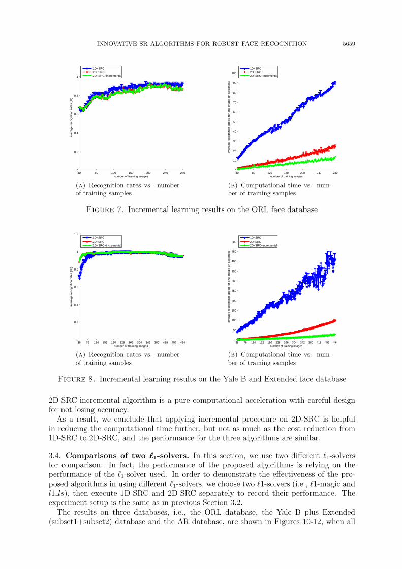
The experimental results on the ORL database, the Yale B plus Extended (subset1+sub-set2) database and the AR database are shown in Figures 7-9 respectively. In each figure,on the left we show the recognition accuracy difference of the three algorithms, whenthe number of training samples increases, and on the right we show their correspondingaverage computational time trends as the number of training samples varies.From the figures, we can see consistently that for all three databases, the 1D-SRC

algorithm always uses the most computational time, the 2D-SRC algorithm use less timethan the 1D-SRC algorithm, and the 2D-SRC-incremental algorithm use the least timeamong three algorithms. The time consuming gap between the 1D-SRC algorithm andthe 2D-SRC algorithm is much bigger that the gap between the 2D-SRC algorithm andthe 2D-SRC-incremental algorithm.Also, the recognition rates of the three algorithms are very close, mostly the 1D-SRC

algorithm is slightly higher than the 2D-SRC algorithm and the 2D-SRC-incremental al-gorithm, but sometimes the contrary is the case. It can be seen that there is nearly no dif-ference of recognition rates between the 2D-SRC algorithm and the 2D-SRC-incrementalalgorithm. This can be expected since the incremental SVD procedure employed in the


40 80 120 160 200 240 2800

0.2

0.4

0.6

0.8

1

number of training images

aver

age

reco

gniti

on r

ates

(%

)

1D−SRC2D−SRC2D−SRC−incremental

(a) Recognition rates vs. numberof training samples

40 80 120 160 200 240 2800

10

20

30

40

50

60

70

80

90

100


ave

rag

e r

eco

gn

itio

n s

pe

ed

fo

r o

ne

ima

ge

(in

se

con

ds)


(b) Computational time vs. num-ber of training samples

Figure 7. Incremental learning results on the ORL face database

38 76 114 152 190 228 266 304 342 380 418 456 4940

0.2

0.4

0.6

0.8

1

1.2


aver

age

reco

gniti

on r

ates

(%

)



38 76 114 152 190 228 266 304 342 380 418 456 4940

50

100

150

200

250

300

350

400

450

500


ave

rag

e r

eco

gn

itio

n s

pe

ed

fo

r o

ne

ima

ge

(in

se

con

ds)



Figure 8. Incremental learning results on the Yale B and Extended face database

2D-SRC-incremental algorithm is a pure computational acceleration with careful designfor not losing accuracy.

As a result, we conclude that applying incremental procedure on 2D-SRC is helpfulin reducing the computational time further, but not as much as the cost reduction from1D-SRC to 2D-SRC, and the performance for the three algorithms are similar.

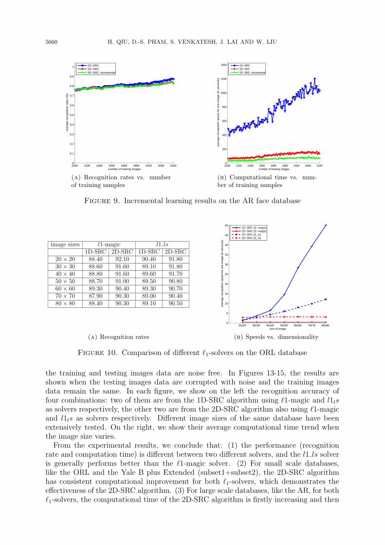
3.4. Comparisons of two ℓ1-solvers. In this section, we use two different ℓ1-solversfor comparison. In fact, the performance of the proposed algorithms is relying on theperformance of the ℓ1-solver used. In order to demonstrate the effectiveness of the pro-posed algorithms in using different ℓ1-solvers, we choose two ℓ1-solvers (i.e., ℓ1-magic andl1 ls), then execute 1D-SRC and 2D-SRC separately to record their performance. Theexperiment setup is the same as in previous Section 3.2.

The results on three databases, i.e., the ORL database, the Yale B plus Extended(subset1+subset2) database and the AR database, are shown in Figures 10-12, when all


1200 1320 1440 1560 1680 1800 1920 2040 21600

0.1

0.2

0.3

0.4

0.5

0.6

0.7

0.8

0.9

1


aver

age

reco

gniti

on r

ates

(%

)



1200 1320 1440 1560 1680 1800 1920 2040 21600

200

400

600

800

1000

1200

1400


ave

rag

e r

eco

gn

itio

n s

pe

ed

fo

r o

ne

ima

ge

(in

se

con

ds)



Figure 9. Incremental learning results on the AR face database

image sizes ℓ1-magic l1 ls1D-SRC 2D-SRC 1D-SRC 2D-SRC

20× 20 88.40 92.10 90.40 91.8030× 30 88.60 91.60 89.10 91.8040× 40 88.80 91.60 89.60 91.7050× 50 88.70 91.00 89.50 90.8060× 60 89.30 90.40 89.30 90.7070× 70 87.90 90.30 89.00 90.4080× 80 88.40 90.30 89.10 90.50


20x20 30x30 40x40 50x50 60x60 70x70 80x80 0

5

10

15

20

25

30

35

40

45

50

size of image

aver

age

reco

gniti

on s

peed

for

one

imag

e (in

sec

onds

)

1D−SRC (l1−magic)2D−SRC (l1−magic)1D−SRC (l1_ls)2D−SRC (l1_ls)

(b) Speeds vs. dimensionality

Figure 10. Comparison of different ℓ1-solvers on the ORL database

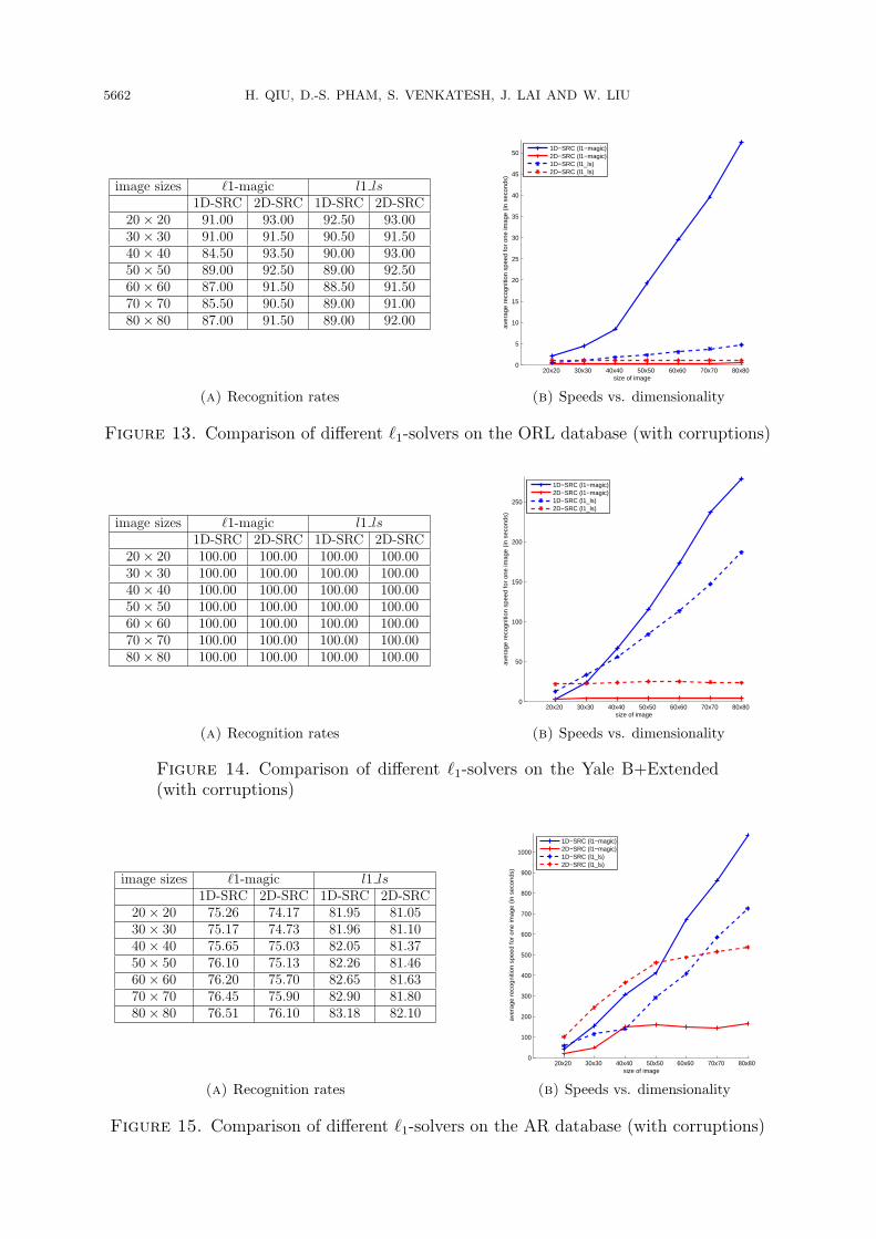
the training and testing images data are noise free. In Figures 13-15, the results areshown when the testing images data are corrupted with noise and the training imagesdata remain the same. In each figure, we show on the left the recognition accuracy offour combinations: two of them are from the 1D-SRC algorithm using ℓ1-magic and l1lsas solvers respectively, the other two are from the 2D-SRC algorithm also using ℓ1-magicand l1ls as solvers respectively. Different image sizes of the same database have beenextensively tested. On the right, we show their average computational time trend whenthe image size varies.From the experimental results, we conclude that: (1) the performance (recognition

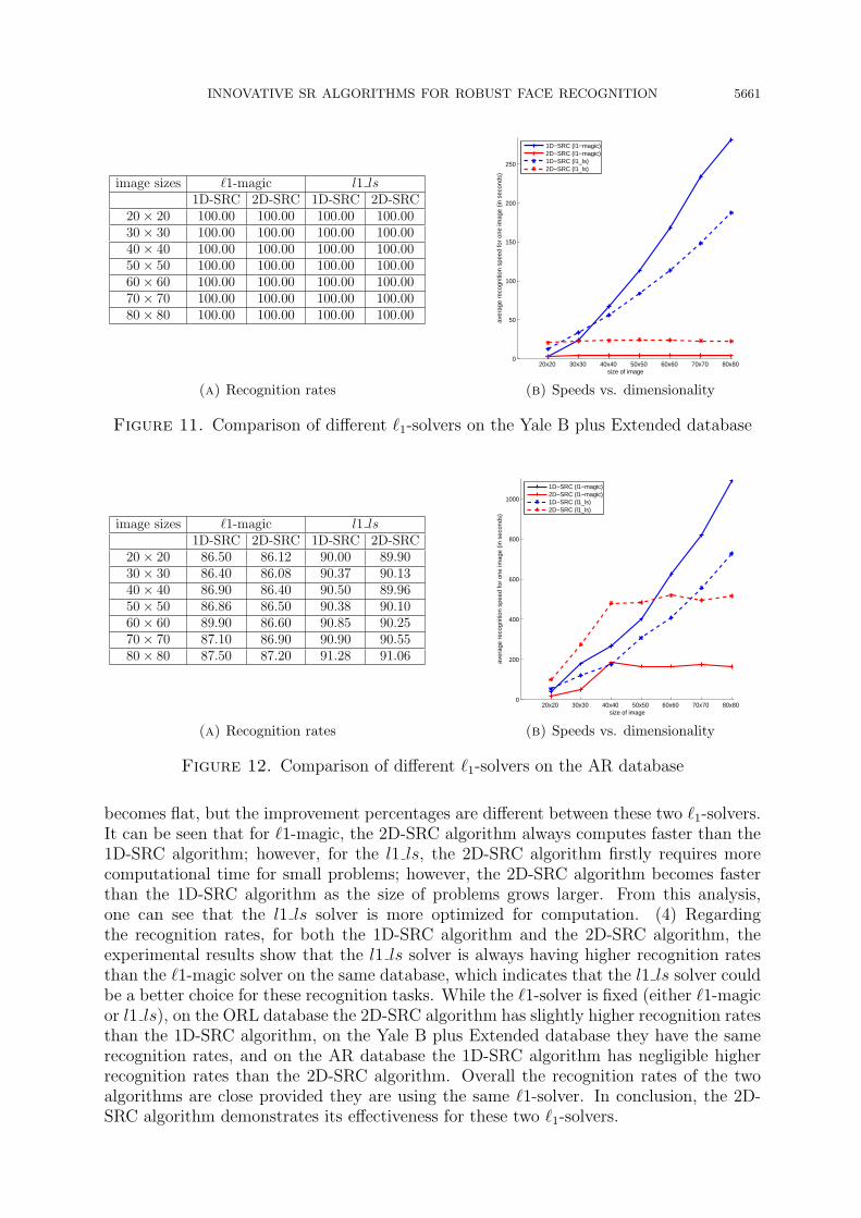
rate and computation time) is different between two different solvers, and the l1 ls solveris generally performs better than the ℓ1-magic solver. (2) For small scale databases,like the ORL and the Yale B plus Extended (subset1+subset2), the 2D-SRC algorithmhas consistent computational improvement for both ℓ1-solvers, which demonstrates theeffectiveness of the 2D-SRC algorithm. (3) For large scale databases, like the AR, for bothℓ1-solvers, the computational time of the 2D-SRC algorithm is firstly increasing and then



20× 20 100.00 100.00 100.00 100.0030× 30 100.00 100.00 100.00 100.0040× 40 100.00 100.00 100.00 100.0050× 50 100.00 100.00 100.00 100.0060× 60 100.00 100.00 100.00 100.0070× 70 100.00 100.00 100.00 100.0080× 80 100.00 100.00 100.00 100.00


20x20 30x30 40x40 50x50 60x60 70x70 80x80 0

50

100

150

200

250

size of image

aver

age

reco

gniti

on s

peed

for

one

imag

e (in

sec

onds

)



Figure 11. Comparison of different ℓ1-solvers on the Yale B plus Extended database


20× 20 86.50 86.12 90.00 89.9030× 30 86.40 86.08 90.37 90.1340× 40 86.90 86.40 90.50 89.9650× 50 86.86 86.50 90.38 90.1060× 60 89.90 86.60 90.85 90.2570× 70 87.10 86.90 90.90 90.5580× 80 87.50 87.20 91.28 91.06


20x20 30x30 40x40 50x50 60x60 70x70 80x80 0

200

400

600

800

1000

size of image

aver

age

reco

gniti

on s

peed

for

one

imag

e (in

sec

onds

)



Figure 12. Comparison of different ℓ1-solvers on the AR database

becomes flat, but the improvement percentages are different between these two ℓ1-solvers.It can be seen that for ℓ1-magic, the 2D-SRC algorithm always computes faster than the1D-SRC algorithm; however, for the l1 ls, the 2D-SRC algorithm firstly requires morecomputational time for small problems; however, the 2D-SRC algorithm becomes fasterthan the 1D-SRC algorithm as the size of problems grows larger. From this analysis,one can see that the l1 ls solver is more optimized for computation. (4) Regardingthe recognition rates, for both the 1D-SRC algorithm and the 2D-SRC algorithm, theexperimental results show that the l1 ls solver is always having higher recognition ratesthan the ℓ1-magic solver on the same database, which indicates that the l1 ls solver couldbe a better choice for these recognition tasks. While the ℓ1-solver is fixed (either ℓ1-magicor l1 ls), on the ORL database the 2D-SRC algorithm has slightly higher recognition ratesthan the 1D-SRC algorithm, on the Yale B plus Extended database they have the samerecognition rates, and on the AR database the 1D-SRC algorithm has negligible higherrecognition rates than the 2D-SRC algorithm. Overall the recognition rates of the twoalgorithms are close provided they are using the same ℓ1-solver. In conclusion, the 2D-SRC algorithm demonstrates its effectiveness for these two ℓ1-solvers.



20× 20 91.00 93.00 92.50 93.0030× 30 91.00 91.50 90.50 91.5040× 40 84.50 93.50 90.00 93.0050× 50 89.00 92.50 89.00 92.5060× 60 87.00 91.50 88.50 91.5070× 70 85.50 90.50 89.00 91.0080× 80 87.00 91.50 89.00 92.00


20x20 30x30 40x40 50x50 60x60 70x70 80x80 0

5

10

15

20

25

30

35

40

45

50

size of image

aver

age

reco

gniti

on s

peed

for

one

imag

e (in

sec

onds

)



Figure 13. Comparison of different ℓ1-solvers on the ORL database (with corruptions)


20× 20 100.00 100.00 100.00 100.0030× 30 100.00 100.00 100.00 100.0040× 40 100.00 100.00 100.00 100.0050× 50 100.00 100.00 100.00 100.0060× 60 100.00 100.00 100.00 100.0070× 70 100.00 100.00 100.00 100.0080× 80 100.00 100.00 100.00 100.00


20x20 30x30 40x40 50x50 60x60 70x70 80x80 0

50

100

150

200

250

size of image

aver

age

reco

gniti

on s

peed

for

one

imag

e (in

sec

onds

)



Figure 14. Comparison of different ℓ1-solvers on the Yale B+Extended(with corruptions)


20× 20 75.26 74.17 81.95 81.0530× 30 75.17 74.73 81.96 81.1040× 40 75.65 75.03 82.05 81.3750× 50 76.10 75.13 82.26 81.4660× 60 76.20 75.70 82.65 81.6370× 70 76.45 75.90 82.90 81.8080× 80 76.51 76.10 83.18 82.10


20x20 30x30 40x40 50x50 60x60 70x70 80x80 0

100

200

300

400

500

600

700

800

900

1000

size of image

aver

age

reco

gniti

on s

peed

for

one

imag

e (in

sec

onds

)



Figure 15. Comparison of different ℓ1-solvers on the AR database (with corruptions)


4. Conclusion. In this paper, we have proposed two fast sparse representation algo-rithms for robust face recognition. One is the 2D-SRC algorithm and the other is anincremental version of 2D-SRC. The main idea for these these two algorithms is basedon the inner product matrix computation, and such computation can be performed inan incremental manner. Experimental results on different benchmark datasets as well asdifferent ℓ1-optimization solvers show that the proposed methods are significantly fasterthan the original SRC algorithm whilst still maintain or even enhance the recognitionrate, especially for large datasets or high-resolution images.

This work is an extension of our previous conference paper in ICPR 2010 [55].

Acknowledgement. The authors thank the anonymous referees for their valuable sug-gestions and helpful comments which help improve the quality of the paper. This projectwas partly supported by the NSFC with grant number U0835005, 60803083, the Guang-dong Program with Grant No. 2009A090100025 and Australia Research Council.

REFERENCES

[1] W. Zhao, R. Chellappa, P. J. Phillips and A. Rosenfeld, Face recognition: A literature survey, ACMComputing Surveys, vol.35, no.4, pp.399-458, 2003.

[2] J. P. Phillips, H. Moon, S. A. Rizvi and P. J. Rauss, The FERET evaluation methodology for face-recognition algorithms, IEEE Transactions on Pattern Analysis and Machine Intelligence, vol.22,no.10, pp.1090-1104, 2000.

[3] A. J. O’Toole, P. J. Phillips and A. Narvekar, FRVT 2002 evaluation report, Technical Report 6965,NISTIR, 2003.

[4] P. J. Phillips, W. T. Scruggs, A. J. O’Toole, P. J. Flynn, K. W. Bowyer, C. L. Schott and M. Sharpe,FRVT 2006 and ice 2006 large-scale experimental results, IEEE Transactions on Pattern Analysisand Machine Intelligence, vol.32, no.5, pp.831-846, 2010.

[5] X. Wang and X. Tang, A unified framework for subspace face recognition, IEEE Transactions onPattern Analysis and Machine Intelligence, vol.26, no.9, pp.1222-1228, 2004.

[6] C.-Y. Chang and H.-R. Hsu, Application of principal component analysis to a radial-basis functioncommittee machine for face recognition, International Journal of Innovative Computing, Informationand Control, vol.5, no.11(B), pp.4145-4154, 2009.

[7] S. D. Lin, J.-H. Lin and C.-C. Chiang, Combining scale invariant feature transform with principalcomponent analysis in face recognition, ICIC Express Letters, vol.3, no.4(A), pp.927-932, 2009.

[8] A. V. Nefian and M. H. Hayess, Hidden markov models for face recognition, The InternationalConference on Acoustics, Speech and Signal Processing, Seattle, Washington, pp.2721-2724, 1998.

[9] B. Moghaddam, Bayesian face recognition, Pattern Recognition, vol.33, no.11, pp.1771-1782, 2000.[10] B. Heisele, P. Ho and T. Poggio, Face recognition with support vector machines: Global versus

component-based approach, The 8th IEEE International Conference on Computer Vision, vol.2,pp.688-694, 2001.

[11] M.-H. Yang, Face recognition using kernel methods, Advances in Neural Information ProcessingSystems, vol.14, pp.1457-1464, 2001.

[12] M.-H. Yang, Kernel eigenfaces vs. kernel fisherfaces: Face recognition using kernel methods, The 5thIEEE International Conference on Automatic Face and Gesture Recognition, Washington, pp.215-220, 2002.

[13] J. Lu, K. N. Plataniotis and A. N. Venetsanopoulos, Face recognition using kernel direct discriminantanalysis algorithms, IEEE Transactions on Neural Networks, vol.14, no.1, pp.117-126, 2003.

[14] J.-B. Li, Nonparametric kernel discriminant analysis for face recognition under varying lightingconditions, ICIC Express Letters, vol.4, no.3(B), pp.999-1004, 2010.

[15] I G. P. S. Wijaya, K. Uchimura and Z. Hu, Face recognition based on dominant frequency features andmultiresolution metric, International Journal of Innovative Computing, Information and Control,vol.5, no.3, pp.641-652, 2009.

[16] L. Wiskott, J. M. Fellous, N. Kuiger and C. von der Malsburg, Face recognition by elastic bunchgraph matching, IEEE Transactions on Pattern Analysis and Machine Intelligence, vol.19, no.7,pp.775-779, 1997.


[17] T. F. Cootes, K. Walker and C. J. Taylor, View-based active appearance models, The 4th IEEEInternational Conference on Automatic Face and Gesture Recognition, pp.227-232, 2000.

[18] V. Blanz and T. Vetter, Face recognition based on fitting a 3d morphable model, IEEE Transactionson Pattern Analysis and Machine Intelligence, vol.25, no.9, pp.1063-1074, 2003.

[19] M. Turk and A. Pentland, Eigenfaces for recognition, Journal of Cognitive Neuroscience, vol.3, no.1,pp.71-86, 1991.

[20] A. M. Martinez and A. C. Kak, PCA versus LDA, IEEE Transactions on Pattern Analysis andMachine Intelligence, vol.23, no.2, pp.228-233, 2001.

[21] P. N. Belhumeur, J. Hespanha and D. J. Kriegman, Eigenfaces vs. fisherfaces: Recognition usingclass specific linear projection, IEEE Transactions on Pattern Analysis and Machine Intelligence,vol.19, no.7, pp.711-720, 1997.

[22] J. Lu, K. N. Plataniotis and A. N. Venetsanopoulos, Face recognition using lda-based algorithms,IEEE Transactions on Neural Networks, vol.14, no.1, pp.195-200, 2003.

[23] X. He, S. Yan, Y. Hu, P. Niyogi and H. J. Zhang, Face recognition using Laplacianfaces, IEEETransactions on Pattern Analysis and Machine Intelligence, vol.27, no.3, pp.328-340, 2005.

[24] S. Yan, D. Xu, B. Zhang, H.-J. Zhang, Q. Yang and S. Lin, Graph embedding and extensions:A general framework for dimensionality reduction, IEEE Transactions on Pattern Analysis andMachine Intelligence, vol.29, no.1, pp.40-51, 2007.

[25] M. S. Bartlett, J. R. Movellan and T. J. Sejnowski, Face recognition by independent componentanalysis, IEEE Transactions on Neural Networks, vol.13, no.6, pp.1450-1464, 2002.

[26] D. D. Lee and H. S. Seung, Learning the parts of objects by non-negative matrix factorization,Nature, vol.401, no.6755, pp.788-791, 1999.

[27] S. Z. Li, X. W. Hou, H. J. Zhang and Q. S. Cheng, Learning spatially localized, parts-based repre-sentation, The IEEE Conference on Computer Vision and Pattern Recognition, vol.1, pp.I-207-I-212,2001.

[28] P. J. Phillips, P. J. Flynn, T. Scruggs, K. W. Bowyer, J. Chang, K. Hoffman, J. Marques, J. Min andW. Worek, Overview of the face recognition grand challenge, The IEEE Conference on ComputerVision and Pattern Recognition, vol.1, pp.947-954, 2005.

[29] P. J. Phillips, P. J. Flynn, T. Scruggs, K. W. Bowyer and W. Worek, Preliminary face recognitiongrand challenge results, The 7th International Conference on Automatic Face and Gesture Recogni-tion, pp.15-24, 2006.

[30] P. J. Phillips, W. T. Scruggs, A. J. O’toole, P. J. Flynn, W. Kevin, C. L. Schott and M. Sharpe,FRVT 2006 and ICE 2006 large-scale results, Technical Report, 2007.

[31] R. Chellappa, P. Sinha and P. J. Phillips, Face recognition by computers and humans, ComputingNow, 2010.

[32] J. Wright, A. Y. Yang, A. Ganesh, S. S. Sastry and Y. Ma, Robust face recognition via sparse rep-resentation, IEEE Transactions on Pattern Analysis and Machine Intelligence, vol.31, no.2, pp.210-227, 2009.

[33] E. J. Candes, J. Romberg and T. Tao, Robust uncertainty principles: Exact signal reconstructionfrom highly incomplete frequency information, IEEE Trans. on Information Theory, vol.52, no.2,pp.489-509, 2006.

[34] D. L. Donoho, Compressed sensing, IEEE Trans. on Information Theory, vol.52, no.4, pp.1289-1306,2006.

[35] H. Zou, T. Hastie and R. Tibshirani, Sparse principal component analysis, Journal of Computationaland Graphical Statistics, vol.15, no.2, 2006.

[36] J. Mairal, M. Elad and G. Sapiro, Sparse representation for color image restoration, IEEE Transac-tions on Image Processing, vol.17, no.1, pp.53-69, 2008.

[37] A. Pagnani, F. Tria and M. Weigt, Classification and sparse-signature extraction from gene-expression data, ArXiv Preprint, 2009.

[38] Rice University, Compressive Sensing Resources, http://dsp.rice.edu/cs.[39] J. J. Fuchs, On sparse representations in arbitrary redundant bases, IEEE Transactions on Infor-

mation Theory, vol.50, no.6, pp.1341-1344, 2004.[40] J.-J. Fuchs, Fast implementation of a ℓ1-ℓ1 regularized sparse representations algorithm, The IEEE

International Conference on Acoustics, Speech, and Signal Processing, pp.3329-3332, 2009.[41] S. Boyd and L. Vandenberghe, Convex Optimization, Cambridge University Press, 2004.[42] R. A. Horn and C. R. Johnson, Matrix Analysis, Cambridge University Press, 1990.[43] D. P. O’Leary and G. W. Stewart, Computing the eigenvalues and eigenvectors of symmetric arrow-

head matrices, Journal of Computational Physics, vol.90, no.2, pp.497-505, 1990.


[44] K. Dickson and T. Selee, Eigenvectors of arrowhead matrices via the adjugate, Preprint, 2007.[45] F. Diele, N. Mastronardi, M. van Barel and E. van Camp, On computing the spectral decomposition

of symmetric arrowhead matrices, Computational Science and Its Applications, LNCS, vol.3044,pp.932-941, 2004.

[46] L. Shen and B. W. Suter, Bounds for eigenvalues of arrowhead matrices and their applications tohub matrices and wireless communications, EURASIP Journal on Advances in Signal Processing,2009.

[47] V. Strassen, Gaussian elimination is not optimal, Numer. Math., vol.13, pp.354-356, 1969.[48] The ORL Database of Faces, AT&T Laboratories Cambridge.[49] A. S. Georghiades, D. J. Kriegman and P. N. Belhurneur, Illumination cones for recognition under

variable lighting: Faces, The IEEE Conference on Computer Vision and Pattern Recognition, pp.52-58, 1998.

[50] K.-C. Lee, J. Ho and D. J. Kriegman, Acquiring linear subspaces for face recognition under variablelighting, IEEE Transactions on Pattern Analysis and Machine Intelligence, vol.27, no.5, pp.684-698,2005.

[51] A. M. Martinez and R. Benavente, The AR face database, CVC Tech. Report #24, 1998.[52] E. Candes and J. Romberg, l1-magic Code, http://www.acm.caltech.edu/l1magic/.[53] S.-J. K. K. Koh and S. Boyd, l1 ls Code, http://www.stanford.edu/ boyd/l1 ls/.[54] S. B. J. Bobin and E. Cands, NESTA Code, http://www.acm.caltech.edu/ nesta/.[55] H. Qiu, D.-S. Pham, S. Venkatesh, W. Liu and J.-H. Lai, A fast extension for sparse representation

on robust face recognition, The 20th International Conference on Pattern Recognition, pp.1023-1027,2010.

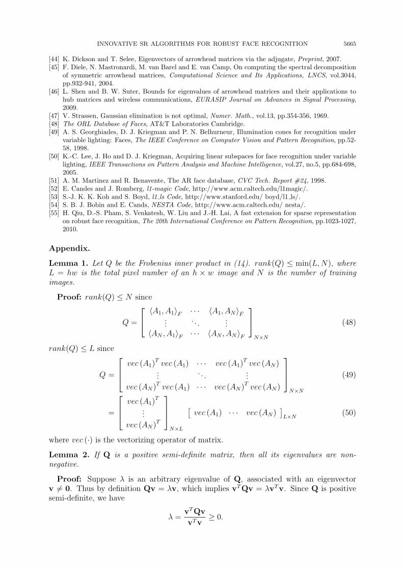
Appendix.

Lemma 1. Let Q be the Frobenius inner product in (14). rank(Q) ≤ min(L,N), whereL = hw is the total pixel number of an h × w image and N is the number of trainingimages.

Proof: rank(Q) ≤ N since

Q =

⟨A1, A1⟩F · · · ⟨A1, AN⟩F...

. . ....

⟨AN , A1⟩F · · · ⟨AN , AN⟩F

N×N

(48)

rank(Q) ≤ L since

Q =

vec (A1)T vec (A1) · · · vec (A1)

T vec (AN)...

. . ....

vec (AN)T vec (A1) · · · vec (AN)

T vec (AN)

N×N

(49)

=

vec (A1)T

...

vec (AN)T

N×L

[vec (A1) · · · vec (AN)

]L×N

(50)

where vec (·) is the vectorizing operator of matrix.

Lemma 2. If Q is a positive semi-definite matrix, then all its eigenvalues are non-negative.

Proof: Suppose λ is an arbitrary eigenvalue of Q, associated with an eigenvectorv = 0. Thus by definition Qv = λv, which implies vTQv = λvTv. Since Q is positivesemi-definite, we have

λ =vTQv

vTv≥ 0.


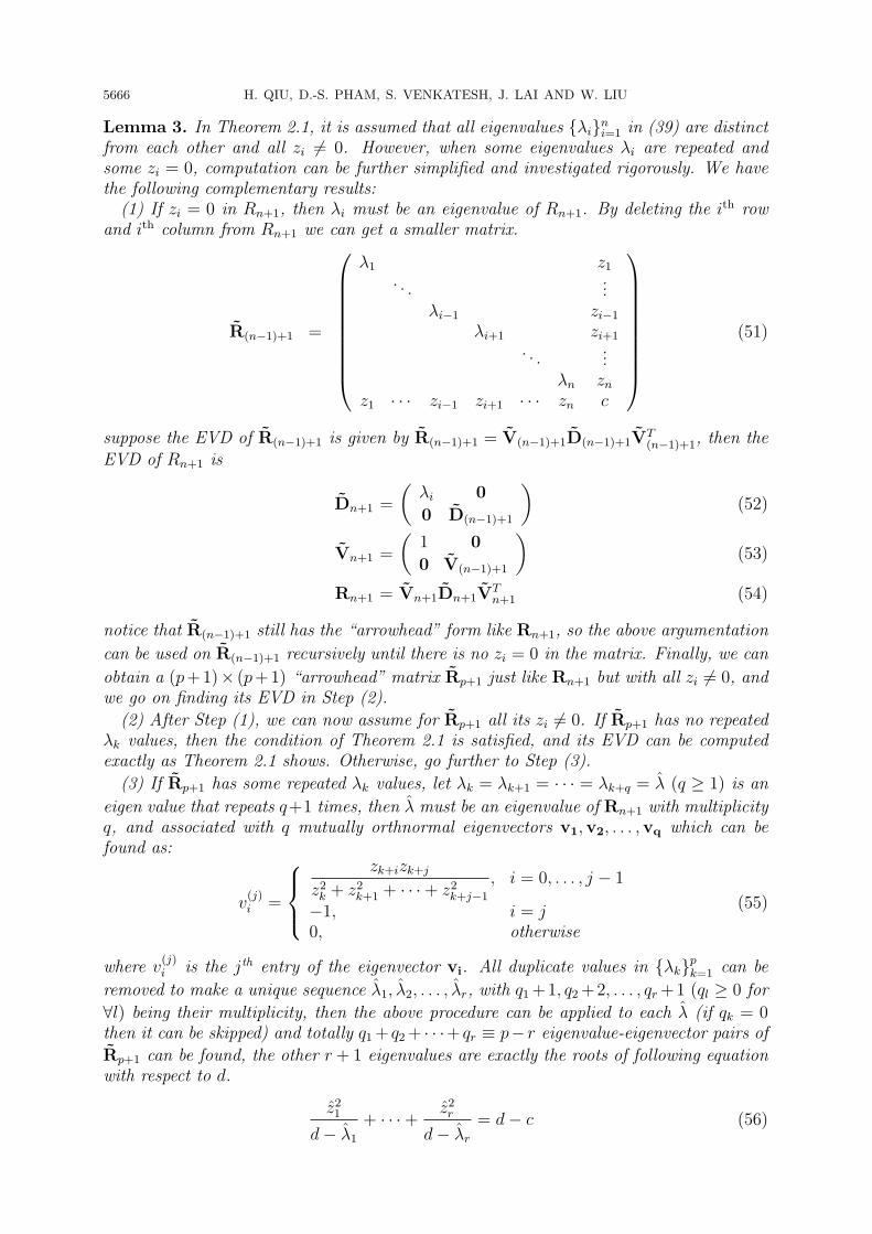
Lemma 3. In Theorem 2.1, it is assumed that all eigenvalues {λi}ni=1 in (39) are distinctfrom each other and all zi = 0. However, when some eigenvalues λi are repeated andsome zi = 0, computation can be further simplified and investigated rigorously. We havethe following complementary results:(1) If zi = 0 in Rn+1, then λi must be an eigenvalue of Rn+1. By deleting the ith row

and ith column from Rn+1 we can get a smaller matrix.

R(n−1)+1 =

λ1 z1. . .

...λi−1 zi−1

λi+1 zi+1

. . ....

λn znz1 · · · zi−1 zi+1 · · · zn c

(51)

suppose the EVD of R(n−1)+1 is given by R(n−1)+1 = V(n−1)+1D(n−1)+1VT(n−1)+1, then the

EVD of Rn+1 is

Dn+1 =

(λi 0

0 D(n−1)+1

)(52)

Vn+1 =

(1 0

0 V(n−1)+1

)(53)

Rn+1 = Vn+1Dn+1VTn+1 (54)

notice that R(n−1)+1 still has the “arrowhead” form like Rn+1, so the above argumentation

can be used on R(n−1)+1 recursively until there is no zi = 0 in the matrix. Finally, we can

obtain a (p+1)× (p+1) “arrowhead” matrix Rp+1 just like Rn+1 but with all zi = 0, andwe go on finding its EVD in Step (2).

(2) After Step (1), we can now assume for Rp+1 all its zi = 0. If Rp+1 has no repeatedλk values, then the condition of Theorem 2.1 is satisfied, and its EVD can be computedexactly as Theorem 2.1 shows. Otherwise, go further to Step (3).

(3) If Rp+1 has some repeated λk values, let λk = λk+1 = · · · = λk+q = λ (q ≥ 1) is an

eigen value that repeats q+1 times, then λ must be an eigenvalue of Rn+1 with multiplicityq, and associated with q mutually orthnormal eigenvectors v1,v2, . . . ,vq which can befound as:

v(j)i =

zk+izk+j

z2k + z2k+1 + · · ·+ z2k+j−1

, i = 0, . . . , j − 1

−1, i = j0, otherwise

(55)

where v(j)i is the jth entry of the eigenvector vi. All duplicate values in {λk}pk=1 can be

removed to make a unique sequence λ1, λ2, . . . , λr, with q1+1, q2+2, . . . , qr+1 (ql ≥ 0 for

∀l) being their multiplicity, then the above procedure can be applied to each λ (if qk = 0then it can be skipped) and totally q1+ q2+ · · ·+ qr ≡ p− r eigenvalue-eigenvector pairs of

Rp+1 can be found, the other r + 1 eigenvalues are exactly the roots of following equationwith respect to d.

z21

d− λ1

+ · · ·+ z2r

d− λr

= d− c (56)


where z2k =∑

ifλi==λk

z2i is the sum of all appearing z2i corresponding to the repeated value

λk. This equation can be solved just like (39) in Theorem 2.1 since it has r + 1 distinctroots d1, d2, . . . , dr. The eigenvector related to dk is the same one given by (41) in Theorem

2.1. So, all (p−r)+(r+1) = p+1 eigenvalues and eigenvectors of Rp+1 can be computednow, even if it has repeated eigenvalues.

(4) All the computations in (1)-(3) are explicitly done by explicit formulas, and theircomplexity is O(n) for computing one eigenvalue and one eigenvector. So, the complexityof finding all eigenvalue and eigenvectors will be O(n2).

Proof: We refer the reader for proving (1)-(3) in [45], and (4) is obvious by checkingeach computation.

Documents

INNOVATIVE SPARSE REPRESENTATION ALGORITHMS FOR ROBUST FACE