Innovative Approaches for Validation of Ultraviolet

1

photo

photo

photo

photo

EPA/600/R-20/094 | April 2020 | www.epa.gov/research

Innovative Approaches for Validation of Ultraviolet Disinfection Reactors for Drinking Water Systems

Office of Research and Development Center for Environmental Solutions and Emergency Response (CESER)

http://www.epa.gov/research

EPA/600/R-20/094

April 2020

ii

Innovative Approaches for Validation of Ultraviolet Disinfection Reactors

for Drinking Water Systems

Prepared by

The Cadmus Group LLC Carol lo Engineers

Under STREAMS Contract No. EP-C-11-039

Off ice of Research and Development Center for Environmental Solut ions and Emergency Response (CESER)

Cincinnat i , OH

iii

Disclaimer The U.S. Environmental Protection Agency, through its Office of Research and Development, funded and managed, or partially funded and collaborated in, the research described herein. It has been subjected to the Agency’s peer and administrative review and has been approved for publication. Any opinions expressed in this report are those of the author (s) and do not necessarily reflect the views of the Agency, therefore, no official endorsement should be inferred. Any mention of trade names or commercial products does not constitute endorsement or recommendation for use.

iv

Foreword The United States Environmental Protection Agency (EPA) is charged by Congress with protecting the Nation's land, air, and water resources. Under a mandate of national environmental laws, the Agency strives to formulate and implement actions leading to a compatible balance between human activities and the ability of natural systems to support and nurture life. To meet this mandate, the EPA's research program is providing data and technical support for solving environmental problems today and building a science knowledge base necessary to manage our ecological resources wisely, understand how pollutants affect our health, and prevent or reduce environmental risks in the future.

The Center for Environmental Solutions and Emergency Response (CESER) within the Office of Research and Development (ORD) conducts applied, stakeholder-driven research and provides responsive technical support to help solve the Nation’s environmental challenges. The Center’s research focuses on innovative approaches to address environmental challenges associated with the built environment. We develop technologies and decision-support tools to help safeguard public water systems and groundwater, guide sustainable materials management, remediate sites from traditional contamination sources and emerging environmental stressors, and address potential threats from terrorism and natural disasters. CESER collaborates with both public and private sector partners to foster technologies that improve the effectiveness and reduce the cost of compliance, while anticipating emerging problems. We provide technical support to EPA regions and programs, states, tribal nations, and federal partners, and serve as the interagency liaison for EPA in homeland security research and technology. The Center is a leader in providing scientific solutions to protect human health and the environment.

Public water systems (PWSs) implement ultraviolet (UV) disinfection for the inactivation of regulated pathogens in accordance with the requirements of the Long Term 2 Enhanced Surface Water Treatment Rule (LT2ESWTR) and the Ground Water Rule (GWR), and the guidance provided by the Ultraviolet Disinfection Guidance Manual (UVDGM). Recreational water facilities (RWFs) install UV systems to improve water sanitation and reduce the likelihood of waterborne diseases such as cryptosporidiosis and giardiasis. UV technologies also provide disinfection and advanced oxidation for potable reuse applications, and there is increased interest in UV technologies to meet the disinfection requirements of the Ground Water Rule (GWR).

Since the UVDGM was published in 2006, there has been considerable advancement in the understanding and application of UV technologies, particularly in the area of UV dose monitoring and validation. This document presents new approaches and procedures for monitoring and validation that leverage these advances, and may reduce the costs and improve the implementation and operation of UV systems for PWSs. The contents of this document meet the requirements of the LT2ESWTR and conform to the underlying principles of the UVDGM. The contents should not be construed as a replacement or revision to the 2006 UVDGM and do not change the UV dose requirements specified in the LT2ESWTR for pathogen inactivation. Validations conducted in accordance with the UVDGM do not need to be re-validated based upon the approaches and procedures presented in this document. These additional approaches and recommendations are presented for consideration when applying UV disinfection for the inactivation of Cryptosporidium, Giardia, and viruses.

v

Table of Contents 1.0 Introduction ...................................................................................................................................... 1

1.1 UV Disinfection Requirements of the LT2ESWTR .................................................................... 2

1.2 Guidance and Challenges with UV Monitoring and Validation .................................................. 2

1.2.1 UV Dose Monitoring .................................................................................................................. 3

1.2.2 RED Bias .................................................................................................................................... 4

1.2.3 Polychromatic Bias and ASCFs ................................................................................................. 7

1.3 Overview of New Approaches for UV monitoring ...................................................................... 8

1.4 Benefits for Regulators and Utilities .......................................................................................... 12

1.5 Document Organization ............................................................................................................. 14

2.0 UV Dose Monitoring Approaches ................................................................................................. 15

2.1 Calculated Dose Approach Using a Combined Variable and a UVT Monitor .......................... 16

2.1.1 Validation Test Plan ................................................................................................................. 17

2.1.2 Functional Testing .................................................................................................................... 20

2.1.3 Analysis of UV Sensor Data..................................................................................................... 21

2.1.4 Biodosimetric Testing .............................................................................................................. 22

2.1.5 Analysis of Biodosimetric Data................................................................................................ 22

2.1.6 Validation Equation QA/QC .................................................................................................... 24

2.1.7 Validated Range ....................................................................................................................... 27

2.1.8 Validation Report ..................................................................................................................... 37

2.2 Calculated Dose Approach Using a Combined Variable and No UVT Monitor ....................... 38

2.2.1 Test Plan ................................................................................................................................... 39

2.2.2 Functional Testing .................................................................................................................... 39

2.2.3 Analysis of UV Sensor Data..................................................................................................... 39


2.2.5 Analysis of Biodosimetric Data................................................................................................ 40

vi

2.2.6 Validated Range ....................................................................................................................... 42


2.3 Calculated Dose Approach with Low and High Wavelength UV Sensors and UVT Monitors 44

2.3.1 Low and High Wavelength Action Spectra Correction Factors ............................................... 46

2.3.2 UV Sensor Properties ............................................................................................................... 48

2.3.3 Test Plan ................................................................................................................................... 49

2.3.4 Functional Testing and Analysis .............................................................................................. 49


2.3.6 Analysis of Biodosimetry Data ................................................................................................ 51

2.3.7 Validated Range ....................................................................................................................... 52


2.4 Calculated Dose Approach with Low and High Wavelength UV Sensors and No UVT Monitors ...................................................................................................................... 55

2.4.1 Test Plan ................................................................................................................................... 56

2.4.2 Functional Testing and Analysis .............................................................................................. 56


2.4.4 Analysis of Biodosimetry Data ................................................................................................ 57

2.4.5 Validated Range ....................................................................................................................... 59


2.5 Hybrid Approaches Using Low and High Wavelength UV Sensors ......................................... 61

2.6 Validation Factors ...................................................................................................................... 61

2.7 UV Dose Requirements .............................................................................................................. 62

2.8 Implementation........................................................................................................................... 63

2.9 Checklists ................................................................................................................................... 66

2.10 Use of Alternate Lamps.............................................................................................................. 73

3.0 General UV Validation and Monitoring Procedures ..................................................................... 74

3.1 Determining UV Dose Response using a Collimated Beam ...................................................... 74

vii

3.2 Test Conditions for the UV Intensity Setpoint Approach .......................................................... 75

3.3 Linear Scaling of Log Inactivation by UV Sensor Readings ..................................................... 76

3.4 Selecting and Applying the RED bias ........................................................................................ 77

3.5 Calculating UDR ........................................................................................................................ 78

3.6 Applying Action Spectra Correction Factors ............................................................................. 82

3.7 Duty UV Sensor Calibration ...................................................................................................... 85

3.8 Online UVT Monitor QA/QC Criteria ....................................................................................... 86

3.9 Lamp-to-Lamp Variability ......................................................................................................... 86

3.10 t-Statistics ................................................................................................................................... 86

3.11 UV Reactors with Enhanced Reflection..................................................................................... 87

3.12 Role of CFD-based UV Dose Models ........................................................................................ 87

4.0 Microbial Methods ......................................................................................................................... 90

4.1 Selecting Challenge Microorganisms......................................................................................... 90

4.2 Preparation of Concentrated Bacteriophage ............................................................................... 91

4.3 Enumeration of Bacteriophage ................................................................................................... 93

4.4 Preparation of Concentrated B. pumilus Spores ........................................................................ 95

4.5 Enumeration of B. pumilus Spores ............................................................................................ 95

4.6 UV Dose Response QA/QC ....................................................................................................... 96

5.0 Future Research Needs ................................................................................................................ 100

6.0 References .................................................................................................................................... 102

Appendix A. Background on Methods ................................................................................................... 106

A.1 UV Dose Distributions and Scaling ......................................................................................... 106

A.2 Evidence to Support the Scaling of the UV Dose Distribution ................................................ 107

A.3 UV Dose Monitoring Using the Combined Variable and a UVT Monitor .............................. 111

A.4 Demonstrating the Combined Variable Approach Using Validation Data .............................. 119

A.5 UV Dose Monitoring Using the Combined Variable and No UVT Monitor ........................... 130

viii

A.6 UV Dose Monitoring with MP UV Systems ............................................................................ 135

A.7 UV Dose Monitoring with MP Systems Using Low and High Wavelength UV Sensors ....... 138

Appendix B. Demonstration Study using an LPHO UV Reactor ........................................................... 147

B.1 TrojanUVSwift™SC D03 ........................................................................................................ 147

B.2 Re-analysis of Validation Data Using the Combined Variable Approach ............................... 148

B.3 Test Bed Treatment Study ........................................................................................................ 151

B.3.1 UV Sensor Equation ......................................................................................................... 152

B.3.2 Collimated Beam Testing ................................................................................................. 154

B.3.3 Biodosimetry Data Analysis ............................................................................................. 157

B.3.3.1 Calculated Dose Approach Using a Combined Variable and a UVT Monitor ............. 157

B.3.3.2 Calculated Dose Approach Using a Combined Variable and No UVT Monitor .......... 161

B.4 Discussion ................................................................................................................................ 163

Appendix C. Demonstration Study using a MP UV Reactor.................................................................. 165

C.1 Xylem-WEDECO Quadron 100............................................................................................... 165

C.2 Test Bed Treatment Study ........................................................................................................ 165

C.2.1 Action Spectra Correction Factors .......................................................................................... 167

C.2.2 Low Wavelength UV Sensors ................................................................................................... 170

C.2.3 UV Sensor Equations ............................................................................................................... 173

C.2.4 UV Sensor QA/QC .................................................................................................................... 179

C.2.5 Collimated Beam Testing ................................................................................................. 182

C.2.6 Biodosimetry Data Analysis .................................................................................................... 185

C.2.6.1 Calculated Dose Approach Using Low and High Wavelength UV Sensors and UVT Monitors 185

ix

Tables Table 1.1: UV Dose Requirements [40 CFR 141.720(d)(1)] ......................................................................2

Table 2.1: Test Plan UVTs for Example 2.1 ..............................................................................................18

Table 2.3: Low and High Wavelength ASCF Values Relative to MS2 Phage .........................................47

Table 2.4: UV Dose (mJ/cm2) for 0.5 to 6.0 log Inactivation of Cryptosporidium, Giardia, and Adenovirus ...............................................................................................................................63

Table 2.5: Coefficients for the Linear Interpolation of UV Sensitivity Based on the UV Dose Values given in Table 2.4 ........................................................................................................64

Table 3.1: MS2 phage UV dose-response data set ....................................................................................80

Table 3.2: UV dose-response uncertainty as a function of log inactivation ..............................................81

Table 3.3: T-statistics for Analyzing Uncertainty with UV Validation Data ............................................87

Table 4.1: Bacteriophage and Hosts for Stock Solution Preparation.........................................................93

Table 4.2: Bacteriophage Stock Propagation Conditions ..........................................................................93

Table 4.3: Bacteriophage and Hosts for Enumeration ...............................................................................94

Table 4.4. Summary of UV Dose-Response Data Used to Define 95th and 99.7th Percentile Prediction Intervals ..................................................................................................................97

Table 4.5. Coefficients for the 95th and 99.7th Percentile Prediction Intervals for the UV Dose- Response of MS2 Phage ..........................................................................................................98

Table 4.6. Coefficients for the 95th and 99.7th Percentile Prediction Intervals for the UV Dose- response of T1UV Phage .........................................................................................................98

Table 4.7 Coefficients for the 95th and 99.7th Percentile Prediction Intervals for the UV Dose- response of T7 Phage ...............................................................................................................98

Table A.1: Evaluation of the Scalability of UV Dose Distributions using CFD-based UV Dose Models where the CFD was Conducted at One Flow ............................................................111

Table A.2: Quality of UV Dose Monitoring Fit to Validation Data Measured with LPHO Lamps ........118

Table A.3: Quality of UV Dose Monitoring Fit to Validation Data Measured with MP Lamps ............119

Table A.4: Low and High Wavelength ASCF Values Relative to MS2 Phage ...................................141

x

Figures Figure 2.1. Comparison of predicted log inactivation. ..............................................................................25

Figure 2.2. Comparison of predicted log inactivation for example 2.2. ....................................................26

Figure 2.3. Validated range of the predicted log inactivation plotted as a function of UVT (Example 1). .............................................................................................................................28

Figure 2.4. Validated range of the predicted log inactivation plotted as a function of UVT (Example 2). .............................................................................................................................29

Figure 2.5. Validated range of the base 10 logarithm of the combined variable, log(CV), plotted as a function of UVT (Example 1). ..........................................................................................30

Figure 2.6. Validated range of the base 10 logarithm of the combined variable, log(CV), plotted as a function of UVT (Example 2). ..........................................................................................31

Figure 2.7. Comparison of the log inactivation calculated using the maximum limit of the combined variable to the maximum limit of predicted log inactivation (Example 1). .............................32

Figure 2.8. Comparison of the log inactivation calculated using the maximum limit of the combined variable to the maximum limit of predicted log inactivation (Example 2). ............33

Figure 2.9. Validated range of the predicted log inactivation plotted as a function of the number of rows of lamps.......................................................................................................................35

Figure 3.1. UVDGM RED Bias Factors for Cryptosporidium Inactivation Credit and a Challenge Microbe UV Sensitivity of 18 to 20 mJ/cm2 per log inactivation............................................78

Figure 3.2. Wavelength response of MS2 phage, T1UV phage, Cryptosporidium, and Adenovirus........83

Figure 3.3. MP lamp output (Linden et al., 2015) and the wavelength response of a UV sensor. ............83

Figure 4.1. 95th and 99.7th percentile prediction intervals for the UV dose response of MS2 phage. .......98

Figure 4.2. 95th and 99.7th Percentile prediction intervals for the UV dose response of T1UV phage. ....99

Figure 4.3. 95th and 99.7th percentile prediction intervals for the UV dose response of T7 phage. ..........99

Figure A.1. Example of a UV dose distribution delivered by a UV reactor predicted using CFD-based UV dose models. .................................................................................................106

Figure A.2. Diagram illustrating the UV intensity model described by Jacob and Dranof (1970). ........108

Figure A.3. Ordered UV dose at various flow rates plotted against ordered UV dose at 5 mgd with a 5 Lamp UV reactor operating at 70 percent UVT and 100 percent lamp power. .......109

Figure A.4. Ordered UV dose at various flow rates plotted against ordered UV dose at 5 mgd with a 5 lamp UV reactor operating at 98 percent UVT and 100 percent lamp power. ........109

Figure A.5. Comparison of observed slopes with Figures A.3 and A.4 with slopes expected with ideal scaling. ..................................................................................................................110

Figure A.6. Relationship between measured log inactivation and log inactivation predicted using CFD-based UV dose models using microbe trajectories predicted at 3 mgd...............111

Figure A.7. Relationship between log inactivation and the combined variable (S/S0)/(Q DL) predicted with CFD-Based UV dose models. ........................................................................113

Figure A.8. Dependence of coefficients A' and B' of Equation A.9 on the UV absorption coefficient. .114

xi

Figure A.9. Relationship between log inactivation predicted by Equation A.12 (x-axis) and the log inactivation predicted using the CFD-Based UV dose model (y-axis) and shown in Figure A.7 ..............................................................................................................................114

Figure A.10. Example showing Equation A.21 providing a better fit than Equation A.9 to the relation between log inactivation and the combined variable (CV) with a UV reactor with a wide dose distribution. ...........................................................................................................116

Figure A.11. Relationship between log inactivation measured with a LPHO UV reactor validation and log inactivation predicted using Equation A.22 (PI = 95th percentile prediction interval). .................................................................................................................................117

Figure A.12. Relationship between log inactivation measured with a LPHO UV reactor validation and log inactivation predicted using Equation A.23 (PI = 95th percentile prediction interval) .................................................................................................................................117

Figure A.13. UV dose response of MS2, T1UV, and T7 phage and A. brasiliensis used to validate the LPHO reactor represented in Figure A.12. .........................................................120

Figure A.14. Measured versus predicted log inactivation by Equation A.23 calibrated using Only MS2, T1UV, and T7 data (PI = 95th percentile prediction interval). .....................................121

Figure A.15. Measured versus predicted log inactivation by Equation A.23 calibrated using only T1UV data where the predictions are limited to the validated range of (S/S0)/(Q DL) with the T1UV data (PI = 95th percentile prediction interval). .............................................121

Figure A.16. Difference between measured and predicted log Inactivation of A. brasiliensis spores as a function of UVT for the combined variable equation fitted to only MS2, T1UV, and T7 validation data. ..............................................................................................123

Figure A.17. Average UV intensity as a function of UVT for the UV reactor represented by Figure A.16. ...........................................................................................................................123

Figure A.18. Comparisons of measured and predicted log inactivation with two commercial LPHO reactors where the validation equation uses a combined variable, (S/S0)/(Q DL) and was fitted to MS2, T1UV, and T7 validation data. .........................................................124

Figure A.19. Comparisons of measured and predicted log inactivation with a commercial MP UV Reactor where the validation equation uses a combined variable, (S/S0)/(Q DL) and was fitted to the validation data measured with S/S0 > 0.8 and used to predict data with S/S0 ranging from 0.3 to 0.8. ..........................................................125

Figure A.20. Comparison of measured and predicted MS2 and T1UV Inactivation by a MP reactor equipped with F240 sleeves where the validation equation uses the combined variable, (S/S0)/(Q DL) (Equation A.12) was fitted to the MS2 validation data. ...................126

Figure A.21. Comparison of measured and predicted MS2 and T1UV inactivation by a MP reactor equipped with F240 sleeves where the validation equation uses the combined variable, (S/S0)/(Q DL), (Equation A.12) and was fitted to the T1UV validation data. ........................126

Figure A.22. Comparison of measured and predicted MS2 and T1UV inactivation by a MP reactor equipped with F240 sleeves where the validation equation uses the combined variable, (S/S0)/(Q DL) (Equation A.12) and was fitted to the validation data with S/S0 less than 0.82.................................................................................................................................................127

Figure A.23. Comparison of measured and predicted MS2 and T1UV inactivation by a MP reactor equipped with F240 sleeves where the validation equation uses the combined variable,

xii

(S/S0)/(Q DL) (Equation A.12) and was fitted to the validation data with S/S0 greater than 0.82.........................................................................................................................................127

Figure A.24. Comparison of log inactivation predicted by the combined variable equation calibrated using T1UV Data (y-axis) to that predicted by the equation calibrated using MS2 data for a MP UV Reactor where 98.29 percent of the predictions are within the 95 th percentile prediction interval. .........................................................................................128

Figure A.25. Comparison of log inactivation predicted by the combined variable equation calibrated using T1UV and T7 Data (y-axis) to that predicted by the equation calibrated using MS2 data for a LPHO UV reactor where all predictions are within the 95 th percentile prediction interval. .................................................................................................................129

Figure A.26. Comparison of log inactivation predicted by the combined variable equation calibrated using T1UV and T7 Data (y-axis) to that predicted by the equation calibrated using MS2 data for a LPHO UV reactor where all predictions are within the 95 th percentile prediction interval. .................................................................................................................129

Figure A.27. Comparison of log inactivation predicted by the combined variable equation calibrated using T1UV and T7 Data (y-axis) to that predicted by the equation calibrated using MS2 data for a MP UV reactor where all predictions are within the 95 th percentile prediction interval. .................................................................................................................130

Figure A.28. Comparison of log inactivation predicted by the combined variable equation calibrated using T1UV and T7 Data (y-axis) to that predicted by the equation calibrated using MS2 data for a MP UV reactor where 98.17 percent of predictions are within the 95 th percentile prediction interval. .........................................................................................130

Figure A.29. Relationship between UV dose and intensity for a UV sensor located (a) at the “Ideal Position,” (b) Close to the Lamp, and (c) far from the lamp. .....................................132

Figure A.30. Relationship between log inactivation and the combined variable S/(Q DL) at various UVTs for different UV sensor to lamp water layer distances with a LPHO reactor. ...........133

Figure A.31. Relationship between measured MS2 REDs and UV sensor divided by flow at various UVTs measured with a MP UV reactor. ...................................................................134

Figure A.32. UV output of a medium pressure UV lamp....................................................................135

Figure A.33. Action spectra of MS2 phage, T1UV phage, Cryptosporidium, and adenovirus. ..........136

Figure A.34. UV transmittance of three quartz sleeve types used by MP UV systems. .....................137

Figure A.35. UV absorption coefficient spectra of five validation test waters with a UVT of 80 percent at 254 nm. .............................................................................................................137

Figure A.36. Spectral response of current commercial UV sensors. ...................................................138

Figure A.37. Comparison of MS2 log inactivation predicted by Equation A.38 (x-axis) to that predicted by CFD-based UV dose models (y-axis) for CFD-predicted validation data with three quartz sleeve types and five validation water types. .............................................142

Figure A.38. Spectral response of low and high wavelength UV sensors used with the analysis Figure A.37. ...........................................................................................................................142

Figure A.39. Comparison of MS2, T1UV, Cryptosporidium, and adenovirus log inactivation predicted by Equation A.38 (x-axis) to that predicted by CFD-based UV dose models

xiii

(y-axis) - Equation A.38 uses low and high wavelength ASCF values given in Table A.4 and was calibrated using the MS2 and T1UV data. ..............................................143

Figure A.40. Comparison of MS2, T1UV, Cryptosporidium, and adenovirus log inactivation predicted by Equation A.38 (x-axis) to that predicted by CFD-based UV Dose Models (y-axis) - Equation A.38 Uses low and high wavelength ASCF values for Cryptosporidium and Giardia Set to 1.0................................................................................144

Figure A.41. Comparison of measured and predicted MS2 and T1UV inactivation by a MP reactor equipped with F240 sleeves where the validation equation uses the combined variable, (S/S0)/(Q DL ASCFH) (Equation A.41) and was fitted to the MS2 validation data. ..............145

Figure A.42. Comparison of measured and predicted MS2 and T1UV inactivation by a MP reactor equipped with F240 sleeves where the validation equation uses the combined variable, (S/S0)/(Q DL ASCFH) (Equation A.41) and was fitted to the T1UV validation data. ............145

Figure A.43. Comparison of measured and predicted MS2 and T1UV inactivation by a MP reactor equipped with F240 sleeves where the validation equation uses the combined variable, (S/S0)/(Q DL ASCFH) (Equation A.41) and was fitted to the validation data with S/S0 less than 0.82. .........................................................................................................................146

Figure A.44. Comparison of measured and predicted MS2 and T1UV inactivation by a MP reactor equipped with F240 sleeves where the validation equation uses the combined variable, (S/S0)/(Q DL ASCFH) (Equation A.41) and was fitted to the validation data with S/S0 greater than 0.82.....................................................................................................................146

Figure B.1. TrojanUVSwift™SC D03 UV reactor. ...........................................................................147

Figure B.2. Measured versus predicted log inactivation using Equation B.1. ..................................148

Figure B.3. Relationship between measured log inactivation and (S/S0)/(Q DL). ................................149

Figure B.4. Measured log inactivation versus predicted log inactivation using Equation B.5 calibrated using the full validation dataset............................................................................149

Figure B.5. Measured log inactivation versus log inactivation by Equation B.5 calibrated using only MS2, T1UV, and T7 data. ....................................................................................150

Figure B.6. UV Dose-response of MS2, T1UV, and T7 phage, A. brasiliensis, and adenovirus .....150

Figure B.7. Measured log inactivation versus predicted log inactivation by Equation B.5 calibrated using only T1UV data. ..........................................................................................151

Figure B.8. UV sensor and adjustable sensor port. ...........................................................................152

Figure B.9. Relationship between the measured and predicted UV intensities at a fixed water layer of 34 mm. ......................................................................................................................153

Figure B.10. Relationship between the measured and predicted UV intensities for all water layers (30 to 59 mm). .............................................................................................................154

Figure B.11. UV Dose-Response of MS2 Phage ...............................................................................155

Figure B.12. UV Dose-Response of B. pumilus Spores .....................................................................156

Figure B.13. UV Dose-Response of Adenovirus ................................................................................156

Figure B.14. Comparison of MS2 UV Dose Response to QA/QC Bounds .............................................157

Figure B.15. Measured vs. predicted log removal with Equation B.14 fitted to MS2 data. ..............160

xiv

Figure B.16. Measured vs. predicted log removal with Equation B.14 fitted to the combined MS2 and B. pumilus data. ......................................................................................................160

Figure B.17. Relationships between measured log I of MS2 phage and S/(Q DL) at water layers of 30, 40, 50, and 60 mm. ...........................................................................................162

Figure B.18. Comparison of log inactivation predicted by Equation B.19 to Measured MS2, B. pumilus, and adenovirus log inactivation. .........................................................................162

Figure C.1. Xylem-Wedeco Quadron 100 UV reactor. .....................................................................165

Figure C.2. UV transmittance for Type 219 and synthetic quartz sleeves. ......................................166

Figure C.3. Comparison of UV dose-response of MS2 phage measured using a collimated beam apparatus equipped with LP and MP lamps. MP UV dose calculated using low and high wavelength ASCF values from Table C.2. ......................................................169

Figure C.4. Comparison of UV dose-response of B. pumilus Spores measured using a collimated beam apparatus equipped with LP and MP lamps. MP UV dose calculated using low and high wavelength ASCF values from Table C.2. .............................................169

Figure C.5a. Comparison of UV dose-response of adenovirus measured using a collimated beam apparatus equipped with LP and MP Lamps. MP UV dose calculated using low and high wavelength ASCF values from Table C.2. ......................................................170

Figure C.5b. Comparison of UV dose-response of adenovirus measured using a collimated beam apparatus equipped with LP and MP lamps. MP UV dose calculated using low and high wavelength ASCF values from Table C.1 .......................................................170

Figure C.6. Spectral response of low wavelength UV sensors. ...........................................................171

Figure C.7. Low wavelength UV sensors have secondary peaks. .......................................................172

Figure C.8. Contribution of different wavelengths to low wavelength UV sensors 1 and 2 readings predicted using UV intensity models. .....................................................................172

Figure C.9. Relationship between the measured and predicted UV intensities for the high wavelength UV sensor. ..........................................................................................................174

Figure C.10. Relationship between the measured and predicted UV intensities for the low wavelength UV Sensor 1. ......................................................................................................174

Figure C.11. Relationship between the measured and predicted UV intensities for the low wavelength UV Sensor 2. ......................................................................................................175

Figure C.12. Relationship between the measured and predicted UV intensities for the high wavelength UV Sensor over various water layers. ................................................................176

Figure C.13. Relationship between the measured and predicted UV Intensities for the low wavelength UV Sensor 2 with synthetic sleeves, sand gravel aquifer as the source water, and super hume as the UV absorber............................................................................178

Figure C.14. Relationship between the measured and predicted UV intensities for the low wavelength UV Sensor 2 with Type 219 Sleeves, Blue Lake Aquifer as the source water, and LSA as the UV absorber.......................................................................................179

Figure C.15a. Relationship between reference and duty high wavelength UV sensor measurements using the synthetic quartz sleeve. ...................................................................180

xv

Figure C.15b. Relationship between reference and duty high wavelength UV sensor measurements using the Type 219 sleeve. .............................................................................180

Figure C.16a. Relationship between Reference and Duty Low Wavelength UV Sensor 1 Measurements using the Synthetic Quartz Sleeve. ................................................................181

Figure C.16b. Relationship between Reference and Duty Low Wavelength UV Sensor 1 Measurements using the Type 219 Sleeve. ............................................................................181

Figure C.17. UV dose-response of MS2 phage (GAP lab). ................................................................183

Figure C.18a. UV dose-response of B. pumilus spores (GAP lab). ...................................................183

Figure C.18b. UV dose-response of B. pumilus Spores (EPA lab). ..................................................184

Figure C.19a. UV dose-response of adenovirus (EPA lab) ...............................................................184

Figure C.19b. UV dose-response of adenovirus (Corona lab). ..........................................................185

Figure C.20. Measured vs predicted log inactivation using Equation C.16 fit to the MS2 data. Equation C.16 used the UVA at 220 nm. Data shown as black triangles likely data outliers. ...........................................................................................................................191

Figure C.21. Measured vs Predicted Log Inactivation using Equation C.16 fit to the MS2 data. Equation C.16 used the UVA at 230 nm. Data shown as black triangles likely data outliers. ...........................................................................................................................192

Figure C.22. Measured vs Predicted Log Inactivation using Equation C.16 fit to the combined MS2 and B. pumilus (GAP lab) data. Equation C.16 used UVA at 220 nm. Data shown as black triangles likely data outliers. ................................................................192

Figure C.23. Measured vs predicted log inactivation using Equation C.16 fit to the MS2 and B. pumilus (EPA lab) data. Equation C.16 used UVA at 220 nm..........................................193

Figure C.24. Measured adenovirus log inactivation from the EPA and corona labs. .........................193

Figure C.25. Comparison of measured and predicted high wavelength UV sensor readings. ................194

Figure C.26. Comparison of measured and predicted low wavelength UV Sensor 2 readings. ..............195

Figure C.27. Linearity of low wavelength UV Sensor 2 readings. ..........................................................196

Figure C.28. Comparison of measured and CFD-predicted MS2 log inactivation. .................................197

Figure C.29. Comparison of measured and CFD-predicted Adenovirus log Inactivation with the Corona lab. .......................................................................................................................198

Figure C.30. Comparison of measured and CFD-predicted Adenovirus log Inactivation with the EPA lab ............................................................................................................................198

Figure C.31. Comparison of measured and CFD-predicted B. pumilus log Inactivation with the GAP lab. ...........................................................................................................................199

Figure C.32. Comparison of measured and CFD-predicted B. pumilus log Inactivation with the EPA lab. ...........................................................................................................................199

Figure C.33. Fraction of log Inactivation Due to Low wavelengths Predicted by Equation C.16 fit to the measured MS2 data (fit includes suspect MS2 data). .............................................200

Figure C.34. Fraction of log inactivation due to Low wavelengths predicted by Equation C.16 fit to the measured MS2 and B. pumilus data (fit excludes suspect MS2 data). ....................200

xvi

Figure C.35. Fraction of log inactivation due to low wavelengths predicted by Equation C.16 fit to the CFD-predicted MS2 data. Equation C.16 predicted log inactivation using low wavelength UV sensor 2 readings calculated using the spectral response from 200 to 240 nm that excluded secondary peaks.......................................................................201

Figure C.36. Comparison of CFD-predicted log inactivation with log inactivation predicted by Equation C.16 fitted to the CFD-predicted MS2 log inactivation. Equation C.16 predicted log inactivation using low wavelength UV sensor 2 readings calculated using the spectral response from 200 to 400 nm including secondary peaks. .......................202

Figure C.38. Spectra response of two hypothetical low wavelength UV sensors with peak response at 228 and 238 nm. ..................................................................................................203

Figure C.39. Comparison of CFD-predicted log inactivation with log inactivation predicted by Equation C.16 fitted to the CFD-predicted MS2 log inactivation. Equation C.16 predicted log inactivation using a low wavelength UV sensor with a peak response at 228 nm................................................................................................................................203

Figure C.40. Comparison of CFD-predicted log inactivation with log inactivation predicted by Equation C.16 fitted to the CFD-predicted MS2 log inactivation. Equation C.16 predicted log inactivation using a low wavelength UV sensor with a peak response at 238 nm................................................................................................................................204

Figure C.41. High Wavelength Component of MS2 Log Inactivation Predicted Using Equation C.16 as a Function of the High Wavelength Combined Variable at Various Water Layers and UVTs at 254 nm. Closed symbols = 219 sleeves, open symbols = synthetic sleeves. ...205

Figure C.42. High wavelength component of B. pumilus log inactivation predicted using Equation C.16 as a function of the high wavelength combined variable at a 45 mm Water Layer. Closed symbols = 219 sleeves, open symbols = synthetic sleeves. .................206

Figure C.43. High wavelength component of adenovirus log inactivation predicted using Equation C.16 as a function of the high wavelength combined variable at a 45 mm Water Layer. Closed symbols = 219 sleeves, open symbols = synthetic sleeves. .................206

Figure C.44. Low wavelength component of MS2 log inactivation predicted using Equation C.16 as a function of the low wavelength combined variable at various water layers and UVTs at 220 nm. Closed symbols = 219 sleeves, open symbols = synthetic sleeves. ..........208

Figure C.45. Low wavelength component of B. pumilus log inactivation predicted using Equation C.16 as a function of the low wavelength combined variable at a 90 mm water layer. closed symbols = 219 sleeves, open symbols = synthetic sleeves. ....................209

Figure C.46. Low wavelength component of adenovirus log inactivation predicted using Equation C.16 as a function of the low wavelength combined variable at a 90 mm water layer. closed symbols = 219 sleeves, open symbols = synthetic sleeves. ..............................209

Figure C.47. Low wavelength Component of Log Inactivation as a Function of the Low Wavelength Combined Variable at a 40 mm Water Layer. Log Inactivation and 228 nm Peak UV Sensor Readings Predicted Using CFD-Based UV Dose Models. Closed symbols = 219 sleeves, open symbols = synthetic sleeves. .......................................210

Figure C.48. Low wavelength Component of Log Inactivation as a Function of the Low Wavelength Combined Variable at a 40 mm Water Layer. Log Inactivation and 238 nm Peak UV Sensor Readings Predicted Using CFD-Based UV Dose Models. Closed symbols = 219 sleeves, open symbols = synthetic sleeves. .......................................211

xvii

xviii

Acronyms and Abbreviations

ASCF Action spectra correction factor ATCC American Type Culture Collection BLA Blue Lake Aquifer CAF Combined Aging and Fouling CESER Center for Environmental Solutions and Emergency Response CFD Computational fluid dynamics CFU Colony forming units CV Combined variable DVGW Deutscher Verein des Gas- und Wasserfaches EPA United States Environmental Protection Agency GWR Ground Water Rule HER Félix d'Hérelle Reference Center ICC-qPCR Integrated Cell Culture Quantitative Polymerase Chain Reaction IUVA International UV Association Log I Log inactivation LP Low pressure LPHO Low pressure high output LSA Lignin sulfonic acid LT2ESWTR Long-Term 2 Enhanced Surface Water Treatment Rule MP Medium pressure NIST National Institute of Standards and Technology NWRI National Water Research Institute ÖNORM Osterreichisches Normungsinstitut QA/QC Quality assurance/quality control PFU Plaque forming unit PLC Programmable logic controller PTB Physikalisch-Technische Bundesanstalt PTFE Polytetrafluorethylene PWS Public Water System RED Reduction equivalent dose RWF Recreational water facility SGA Sand and Gravel Aquifer STREAMS Scientific, Technical, Research, Engineering, and Modeling Support TNTC Too numerous to count TSA Tryptic soy agar TSB Tryptic soy broth TTC Triphenyl tetrazolium chloride TYGA Tryptone Yeast Extract Glucose Agar UV Ultraviolet UVA UV Absorption UVDGM UV Disinfection Guidance Manual UVT UV Transmittance WRF Water Research Foundation WTP Water Treatment Plant WWTP Wastewater Treatment Plant

https://www.ptb.de/cms/en.html

xix

Authors and Contributors Authors

• Harold Wright, Carollo Engineers • Traci Brooks, Carollo Engineers • Mark Heath, Carollo Engineers

Project Managers

• Jeff Adams, US EPA Office of Research and Development • Sam Hayes, US EPA Office of Research and Development • Sally Gutierrez, US EPA Office of Research and Development • Thomas Speth, US EPA Office of Research and Development • Linda Hills, The Cadmus Group LLC • Mark Heath, Carollo Engineers

Contributors and Reviewers

• Karl Linden, University of Colorado • James Malley, University of New Hampshire • Laura Dufresne, The Cadmus Group LLC • Thomas Hargy, Corona Environmental Consulting • Charles Gerba, University of Arizona • Bryan Townsend, Black & Veatch • Jim Bolton, Bolton Photosciences Inc. • Chengyue Shen, HDR, Inc. • Michael Finn, US EPA Office of Water • Derek Losh, US EPA Office of Water • Keith Bircher, Calgon Carbon Corporation • Christian Bokermann, Xylem-WEDECO • Yuri Lawryshyn, University of Toronto • John D. Paccione, New York State Department of Health and the University at Albany • Ronald Gehr, McGill University • Ian Mayor-Smith, University of Brighton • Gord Knight, Trojan Technologies • Steve McDermid, Trojan Technologies • Mike Sasges, Trojan Technologies • Greg Warkentin, Trojan Technologies • Stewart Hayes, Trojan Technologies • Ted Mao, Trojan Technologies • Linda Gowman, Trojan Technologies • Steve Via, American Water Works Association • Phyllis Posy - Atlantium Technologies • Alice Fullmer - Water Research Foundation • Eva Nieminski - Utah Department of Environmental Quality

xx

Laboratory Contributors

• Laura Boczek, US EPA Office of Research and Development • Hodon Ryu, US EPA Office of Research and Development • Eric Rhodes, US EPA Office of Research and Development • Jill Hoelle, US EPA Office of Research and Development • Jonathan Popovicci, US EPA Office of Research and Development • Jennifer Cashdollar, US EPA Office of Research and Development • Emma Huff, US EPA Office of Research and Development • Mark Rodgers, US EPA Office of Research and Development • Ann Grimm, US EPA Office of Research and Development • GAP EnviroMicrobial Services Ltd. • TetraTech, Inc. • Analytical Services, Inc.

UV Reactor Manufacturers

• Xylem-WEDECO • Trojan Technologies

The authors wish to acknowledge and thank the International Ultraviolet Association (IUVA) for leading and managing the technical review for this report.

xxi

Executive Summary

Public water systems (PWSs) implement ultraviolet (UV) disinfection for the inactivation of regulated pathogens in accordance with the requirements of the Long Term 2 Enhanced Surface Water Treatment Rule (LT2ESWTR) and the Ground Water Rule (GWR), and the guidance provided by the Ultraviolet Disinfection Guidance Manual (UVDGM). Recreational water facilities (RWFs) install UV systems to improve water sanitation and reduce the likelihood of waterborne diseases such as cryptosporidiosis and giardiasis. UV technologies also provide disinfection and advanced oxidation for potable reuse applications, and there is increased interest in UV technologies to meet the disinfection requirements of the Ground Water Rule (GWR).

Since the UVDGM was published in 2006, there has been considerable advancement in the understanding and application of UV technologies, particularly in the area of UV dose monitoring and validation. This document presents new approaches and procedures for monitoring and validation that leverage these advances. These approaches and procedures include:

• Microbial methods and dose-response QA/QC bounds for commonly used microbial surrogates in UV reactor validation;

• Approaches for the development of calculated UV dose monitoring algorithms with improved accuracy that eliminate the need for RED bias factors;

• Approaches for the development of UV dose monitoring algorithms that do not require an online UV transmittance monitor for simplified UV system operations;

• For UV reactors equipped with medium pressure UV lamps, implementation of “low wavelength” UV sensors and approaches for the development of UV dose monitoring algorithms that account for the disinfection associated with wavelengths below 240 nm;

• Criteria for the development of a robust validation test matrix, monitoring algorithm goodness of fit and QA/QC requirements, and standardized approaches for defining the validated range of UV reactors;

• Target UV doses for 4.5, 5.0, 5.5 and 6.0 log inactivation of Cryptosporidium, Giardia and virus for UV applications requiring higher levels of disinfection than the maximum 4.0 log provided by the UVDGM;

• General validation and data analysis procedures that are commonly implemented in UV reactor validation but are not explicitly documented in the UVDGM;

• Modifications to the operating recommendations of the UVDGM to improve the accuracy of UV dose-monitoring with the water treatment application.

xxii

The contents of this document meet the requirements of the LT2ESWTR and conform to the underlying principles of the UVDGM. The contents should not be construed as a replacement or revision to the 2006 UVDGM and do not change the UV dose requirements specified in the LT2ESWTR for pathogen inactivation. Validations conducted in accordance with the UVDGM do not need to be re-validated based upon the approaches and procedures presented in this document. These additional approaches and recommendations are presented for consideration when applying UV disinfection for the inactivation of Cryptosporidium, Giardia, and viruses. A detailed description regarding the development of these additional approaches is presented in Appendix A. Case studies evaluating these approaches with UV systems that use low pressure high output (LPHO) and medium pressure (MP) UV lamps are presented in Appendices B and C, respectively. Lessons learned from the case studies were used to refine the approaches described in Sections 2, 3, and 4 of this document. For a thorough understanding of this report’s content, a review of these appendices is highly recommended.

The audience for this document includes UV system manufacturers, validators, consultants, utilities, and regulators. Detailed information is presented for defining, validating, and implementing four new calculated dose monitoring algorithms. These approaches may provide utilities with more cost-effective and robust implementation of UV disinfection. In addition, checklists and validation report outlines are presented to assist Regulators in approving UV systems. This document also provides recommendations on general procedures and reference documentation that support approaches currently being used but not documented in the UVDGM for validating and operating a UV system.

The 2006 UVDGM describes two approaches for UV dose monitoring, namely the UV intensity setpoint approach and the calculated dose approach. While the UV intensity setpoint and its validation were well-defined when the UVDGM was published, there was less information and experience on how to implement the calculated dose approach. This knowledge gap has since been addressed through projects funded through the Water Research Foundation (WRF) as well as extensive experience with validation testing conducted by UV system manufacturers.

With the calculated dose approach, data collected during UV validation testing are analyzed to define an equation that predicts microbe inactivation and the associated reduction equivalent dose (RED) as a function of the flow rate through the reactor (Q), the UV transmittance (UVT) of the water,1 and the UV output of the lamps (S/S0) determined using UV sensor readings (S). To account for the uncertainty of monitoring algorithms developed through UV validation testing, the RED is divided by a validation factor to define the validated UV dose. The validated UV dose is compared to the UV dose requirements of the LT2ESWTR to define pathogen inactivation credit.

This document describes four methods for implementing the calculated dose approach. The first method predicts microbe log inactivation as a function of UVT and a combined variable that is defined as (S/S0)/(Q DL) where DL is the UV dose per log inactivation of the microbe whose log inactivation is being predicted. The use of the combined variable is the primary advancement that has a number of benefits for PWSs and state regulators. By setting the value of DL with the

1 Unless otherwise noted, UVT is at 254 nanometers (nm).

xxiii

combined variable to that of the target pathogen, the RED bias factor specified by the UVDGM and included within the validation factor can be set to a value of 1.0, which simplifies UV dose monitoring and provides more cost-effective selection and implementation of UV technologies.

In concept, the equation can be calibrated using validation data obtained using one challenge microorganism, such as MS2 phage, and then used to directly predict the log inactivation of the regulated pathogens, namely Cryptosporidium, Giardia, and viruses. In practice, this document recommends calibrating the equation using a validation dataset collected using two or more challenge microorganisms with different UV dose-response, such as MS2 and T1UV phage. The validation report should provide an analysis that shows that the equation calibrated using MS2 phage predicts T1UV log inactivation and vice versa. This analysis will provide confidence that the calculated dose approach using the combined variable can directly predict the log inactivation of the targeted or regulated pathogen effectively. While using multiple microbes whose UV dose-response curves bracket the UV dose-response curve of the target pathogen is not discouraged, the studies conducted for this research demonstrate that bracketing is not necessary with calculated dose approaches that use the combined variable.

The second calculated dose approach method predicts microbe log inactivation as a function of a combined variable defined as S/(Q DL) where S is the UV intensity measured by the UV sensor. This approach does not employ an online UVT monitor and provides effective monitoring if the UV sensor is optimally located within the reactor. This document provides recommendations on how to determine that location through validation testing.2 Though this method does not use UVT to determine UV dose delivery by the UV reactor, utilities using UV disinfection should regularly monitor the UVT of their water and take actions as needed to keep the UVT above the value used as the design criterion for their UV system.

These two methods can be used with UV reactors equipped with LP, LPHO, and MP UV lamps. The third and fourth methods, described in the following paragraphs, are focused only on MP lamp systems.

Compared to LP and LPHO lamps that emit UV light at one wavelength, namely 253.7 nm, MP UV lamps emit germicidal UV light at wavelengths from 200 to 300 nm. The UVDGM3 states that the validation factor for UV systems using MP lamps should include action spectra correction factors (ASCFs) to account for differences in the wavelength response of the challenge microorganisms used to validate the UV reactor and the target pathogens (Linden et al., 2015). Since the UVDGM was published, research has shown important differences between the wavelength response of challenge microorganisms and target pathogens at wavelengths below 240 nm. If the validation factor did not include an ASCF to account for these differences, the UV dose monitoring equation may overestimate the inactivation of Cryptosporidium and Giardia and under- or overestimate the inactivation of adenovirus (Linden et al., 2015).

The method of determining the value of the ASCF in the UVDGM is conservative for many UV reactors, thereby increasing the costs for installing UV disinfection. To address this issue, the WRF sponsored Project 4376 entitled "Guidance for Implementing Action Spectra Correction

2 See Section 2.2 of this document. 3 See Section D.4.1 of the UVDGM.

xxiv

with Medium Pressure UV Disinfection" (Linden et al., 2015). This project developed tables of ASCF values that could be broadly applied to MP UV reactors and developed guidance for using UV dose models based on computational fluid dynamics (CFD) to calculate ASCF values specific to a UV reactor and its validation. However, because commercial MP UV reactors use UV sensors that do not monitor wavelengths below 240 nm, the approach used by Linden et al. (2015) to determine ASCFs does not allocate credit for any pathogen inactivation below 240 nm.

For UV systems using MP UV lamps, this document describes a third calculated dose approach method that uses both low and high wavelength UV sensors4 to monitor the contribution to UV dose delivery by wavelengths below and above 240 nm, respectively. With this approach, the microbe log inactivation is predicted as the sum of low wavelength (i.e., wavelengths < 240 nm) and high wavelength (i.e., wavelengths > 240 nm) log inactivation contributions. The high wavelength component is predicted as a function of UVT at 254 nm and a high wavelength combined variable defined as (SH/S0H)/(Q DL ASCFH) where SH/S0H is the lamp output defined by a high wavelength UV sensor and ASCFH is a high wavelength ASCF. Similarly, the low wavelength component is predicted as a function of a low wavelength UVT and a low wavelength combined variable defined as (SL/S0L)/(Q DL ASCFL) where SL/S0L is the lamp output defined by a low wavelength UV sensor and ASCFL is a low wavelength ASCF. The low and high wavelength ASCF values are fixed values calculated using the UV output of the lamp and the action spectra of the challenge microorganism and the target pathogen, or determined experimentally using a collimated beam apparatus equipped with MP lamps. While this approach requires a low wavelength UV sensor and UVT monitor, thereby increasing the complexity of UV dose monitoring and validation, it has the advantage of accounting for target pathogen inactivation at wavelengths below 240 nm, which can reduce the capital and operating costs of UV disinfection. In particular, PWSs could realize a significant reduction in lamp and power costs when MP UV systems are used for adenovirus inactivation credit. The approach also simplifies the application of ASCF values since CFD-based UV dose models are not required to determine low and high wavelength ASCFs.

For the fourth calculated dose approach method, if the low and high wavelength UV sensors are both optimally located, the low and high wavelength components of log inactivation, respectively, can be predicted as a function of a low wavelength combined variable SL/(Q DL ASCFL) and a high wavelength combined variable SH/(Q DL ASCFH). With this method, online UVT monitors are not employed. A hybrid method5 can also be defined where the high wavelength component is defined as a function of the UVT at 254 nm and the high wavelength combined variable (SH/S0H)/(Q DL ASCFH) and the low wavelength component is defined as a function of the low wavelength combined variable SL/(Q DL ASCFL) using an optimally placed low wavelength UV sensor. This hybrid method eliminates the need for an online UVT monitor for low wavelengths.

This document also provides recommendations on general procedures and reference documentation that support approaches currently being used but not documented in the UVDGM

4 A low wavelength UV sensor has a peak response below 240 nm while the high wavelength UV sensor has a peak response near 260 nm. 5 See Section 2.5 of this document.

xxv

for validating and operating a UV system, including: improved approaches for analyzing challenge microorganism UV dose response data measured using a collimated beam apparatus; UV dose values for up to 6-log inactivation of Cryptosporidium, Giardia and adenovirus; clarifications on determining the validation factor; improved quality control for UV sensors and UVT monitors when the UV system operates at the PWS; methods for using challenge microorganisms other than MS2 phage for UV validation; and the provision of Quality Assurance/Quality Control (QA/QC) bounds for the UV dose-response of MS2, T1UV, and T7 phage.

1

1.0 Introduction Since the discovery that ultraviolet (UV) light inactivates Cryptosporidium and Giardia at relatively low UV doses (Bukhari et al., 1999; Craik et al., 2000), over 300 public water systems (PWSs) in North America have implemented UV disinfection at flows up to 2,200 million gallons per day (MGD) (Wright et al., 2012). Many of those UV systems were implemented in accordance with the requirements of the Long Term 2 Enhanced Surface Water Treatment Rule (LT2ESWTR) and the guidance provided by the Ultraviolet Disinfection Guidance Manual (UVDGM) (USEPA, 2006). Recreational water facilities (RWFs) have also implemented UV disinfection in response to epidemiological studies that have shown that cryptosporidiosis represents a disproportionately large fraction of all recreational water illnesses (Paccione et al., 2017). UV technologies also provide disinfection and advanced oxidation for potable reuse applications, and there is increased interest in UV technologies to meet the disinfection requirements of the Ground Water Rule (GWR).

Since the UVDGM was published in 2006, there has been considerable advancement in the understanding and application of UV technologies, particularly in the area of UV dose monitoring and validation. This document presents new methods for UV dose monitoring and validation that leverage these advances, and may reduce the costs and improve the implementation and operation of UV systems for PWSs. The contents of this document meet the requirements of the LT2ESWTR and conform to the underlying principles of the UVDGM. The contents should not be construed as a replacement or revision to the 2006 UVDGM and do not change the UV dose requirements specified in the LT2ESWTR for pathogen inactivation. Validations conducted in accordance with the UVDGM do not need to be re-validated based upon the approaches and procedures presented in this document. These additional approaches and recommendations are presented for consideration when applying UV disinfection for the inactivation of Cryptosporidium, Giardia, and viruses. A detailed description regarding the development of these additional approaches is presented in Appendix A. Case studies evaluating these approaches with UV systems that use LPHO and MP UV lamps are presented in Appendices B and C, respectively. Lessons learned from the case studies were used to refine the approaches described in Sections 2, 3, and 4 of this document. For a thorough understanding of this report’s content, a review of these appendices is highly recommended.

The audience for this document includes UV system manufacturers, validators, consultants, utilities, and regulators. Detailed information is presented for defining, validating, and implementing four new calculated dose monitoring algorithms. These algorithms may provide utilities with more cost-effective and robust implementation of UV disinfection. In addition, checklists and validation report outlines are presented to aid Regulators in approving systems. Chapter 3 of this document also provides general recommendations for UV dose monitoring and validation that build on the recommendations provided by the UVDGM.

This chapter covers:

1.1 UV Disinfection Requirements of the LT2ESWTR;

1.2 Guidance and Challenges with UV Monitoring and Validation;

1.3 Overview and Benefits of New Approaches for UV Monitoring; and

1.4 Document Organization.

2

1.1 UV Disinfection Requirements of the LT2ESWTR

The United States Environmental Protection Agency (EPA) developed the LT2ESWTR to further improve and protect the microbiological quality of drinking water. The rule provides UV dose requirements for 0.5 to 4.0 log inactivation of Cryptosporidium, Giardia, and viruses (Table 1.1) applicable for unfiltered systems as well as post-filter applications of UV disinfection with filtered systems. The UV dose requirements for viruses are based on the UV dose-response of adenovirus, recognized as the most UV-resistant waterborne viral pathogen. Adenovirus is resistant to UV light because UV-induced DNA damage in the virus is repaired by host cell mechanisms (Arnold and Rainbow, 1996).

The LT2ESWTR requires that PWSs use UV reactors that have undergone validation testing. UV validation must involve testing of a full-scale UV reactor that conforms uniformly to the UV reactors used by the PWS in terms of wetted dimensions and optical properties that impact UV dose delivery and monitoring. The validation must demonstrate inactivation by the UV reactor of a test microorganism whose dose-response characteristics have been quantified with a LP mercury vapor lamp. The validation testing must determine the operating conditions under which the reactor delivers the required UV dose for treatment credit [40 CFR 141.720(d)(2)]. These operating conditions must include flow rate, UV intensity as measured by a UV sensor, and UV lamp status, and must account for the UV absorption coefficient of the water, lamp fouling and aging, measurement uncertainty of online sensors, UV dose distributions arising from the velocity profiles through the reactor, failure of UV lamps or other critical system components, and inlet and outlet piping or channel configurations of the UV reactor.

The LT2ESWTR requires PWSs to monitor their UV reactors to demonstrate that they are operating within the range of conditions that were validated for the required UV dose [40 CFR 141.720(d)(3)(i)]. At a minimum, PWSs must monitor each reactor for flow rate, lamp status, UV intensity as measured by a UV sensor, and any other parameters required by the state. UV transmittance (UVT) should also be measured when it is used in a UV dose-monitoring strategy. PWSs must verify the calibration of UV sensors and recalibrate sensors in accordance with a protocol that the state approves. To receive disinfection credit for UV, both filtered and unfiltered PWSs must treat at least 95 percent of the water delivered to the public during each month by UV reactors operating within validated conditions for the required UV dose [40 CFR 141.720(d)(3)(ii)]. The PWS must provide initial reporting to the state on validation test results as well as routine reporting on UV dose monitoring [40 CFR 141.721(f)(15)].

Table 1.1: UV Dose Requirements [40 CFR 141.720(d)(1)] UV dose (mJ/cm2) for an inactivation of:

0.5 log 1.0 log 1.5 log 2.0 log 2.5 log 3.0 log 3.5 log 4.0 log

Cryptosporidium 1.6 2.5 3.9 5.8 8.5 12 15 22

Giardia lamblia 1.5 2.1 3.0 5.2 7.7 11 15 22

Virus 39 58 79 100 121 143 163 186

1.2 Guidance and Challenges with UV Monitoring and Validation

To support the implementation of UV disinfection in accordance with the LT2ESWTR, the EPA developed the UVDGM (USEPA, 2006). The UVDGM provides an overview of UV disinfection and guidance for UV system planning, design, validation, startup, and operation. It is recommended that those who are considering the new concepts, protocols, and enhanced procedures described in this report should understand the requirements of the LT2ESWTR and the recommendations of the UVDGM.

3

Documentation in this report provides clarifications on approaches provided by the UVDGM and enhanced procedures for consideration, based on the advances achieved in the UV industry that occurred after the UVDGM was published. The contents of this document should not be construed as a replacement or revision to the 2006 UVDGM, but rather additional approaches and procedures for consideration when applying UV disinfection for the inactivation of Cryptosporidium, Giardia, and viruses.

Chapter 5 of the UVDGM provides a recommended validation protocol. With UV validation, a manufacturer installs a UV reactor representative of a product line into a test train. The reactor is operated over a range of flow rates, water UVT, and lamp power settings. At each test condition, a challenge microorganism is injected into the flow upstream of the reactor and the log inactivation of that challenge microorganism by the reactor is measured. In parallel, the UV dose-response of the challenge microorganism is measured using a collimated beam apparatus. The UV dose response is then used to relate the log inactivation of the challenge microorganism to a UV dose value, referred to as the reduction equivalent dose (RED). The resulting dataset is analyzed to define a UV dose monitoring algorithm for the UV reactor.

1.2.1 UV Dose Monitoring

The UVDGM describes two approaches for UV dose monitoring: the UV intensity setpoint approach and the calculated dose approach.

The UV intensity setpoint approach is based on the monitoring approach specified by the German (DVGW, 2006) and Austrian (ÖNORM, 2001; ÖNORM. 2003) UV regulations and guidance developed in the 1990s. As such, the approach and its validation are well-defined. With the UV intensity setpoint approach, the UV reactor delivers a required UV dose when the UV intensity measured by the UV sensor is greater than or equal to a setpoint value that is defined as a function of the flow rate through the UV reactor.

With the calculated dose approach, validation test data is used to develop an equation that predicts the RED delivered by the reactor as a function of the flow rate through the reactor, the UVT of the water being treated, and the UV intensity measured by UV sensors.

When the UVDGM was being prepared, there had not been much experience developing equations for the calculated dose approach using validation data. The UVDGM states that the following empirical equation can provide a good fit to validation data:

𝑅𝑅𝑅𝑅𝐷𝐷 = 10𝑎𝑎 × 𝐴𝐴254𝑏𝑏 × �𝑆𝑆 𝑆𝑆0� �𝑐𝑐

× �1𝑄𝑄� �

𝑑𝑑× 𝐵𝐵𝑒𝑒 Equation 1.1

where:

RED = Reduction equivalent dose calculated with the dose-monitoring equation

A254 = UV absorption coefficient at 254 nm (cm-1, m-1)

S = Measured UV sensor value (mW/cm2, W/m2)

So = UV sensor value at 100 percent lamp power with new lamps and clean sleeves, typically expressed as a function of UVT (mW/cm2, W/m2)

Q = Flow rate (mgd, gpm, MLD, m3/s, etc.)

B = Number of operating banks of lamps within the UV reactor

4

a, b, c, d, e = Model coefficients obtained by fitting the equation to the data However, the UVDGM provides no rationale for why this equation should provide a good fit to the relationships between RED and the independent variables of flow rate, UV absorption coefficient, UV sensor readings, and banks of lamps; the equation is empirical.

1.2.1.1 Validation Factor The UVDGM states that the validated dose delivered by the reactor is defined as:

𝑉𝑉𝑉𝑉𝑉𝑉𝑉𝑉𝑉𝑉𝑉𝑉𝑡𝑡𝑡𝑡𝑉𝑉 𝐷𝐷𝐷𝐷𝐷𝐷𝑡𝑡 = 𝑅𝑅𝑅𝑅𝐷𝐷𝑉𝑉𝑉𝑉� Equation 1.2

where:

VF = Validation factor The validated dose is compared to the UV dose requirements (Table 1.1) for defining disinfection credit achieved by the UV reactor.

The validation factor accounts for uncertainties and biases that occur when experimental testing is used to define the validated dose delivered by the reactor. The UVDGM states that the validation factor is defined as:

𝑉𝑉𝑉𝑉 = 𝐵𝐵𝑅𝑅𝑅𝑅𝑅𝑅 × 𝐵𝐵𝑃𝑃𝑃𝑃𝑃𝑃𝑃𝑃 × �1 + 𝑉𝑉𝑉𝑉𝑉𝑉100

� 𝑈𝑈 Equation 1.3

where:

BRED = RED bias factor

BPoly = Polychromatic bias factor

UVal = Uncertainty of validation expressed as a percentage of the RED

1.2.2 RED Bias

Because UV reactors deliver a UV dose distribution, the RED depends on the UV dose-response of the microorganism being inactivated (Cabaj et al., 1996). The RED bias is defined as the ratio of the RED measured using the challenge microorganism used to validate the reactor and the RED that would have been delivered to the target pathogen. If the challenge microorganism has the same UV dose-response as the target pathogen, as defined by the UV dose-requirements of the LT2ESWTR, the RED bias is 1.0. If the challenge microorganism is more resistant to UV light than the target pathogen, the RED bias is greater than 1.0. If the challenge microorganism is more sensitive to UV light than the target pathogen, the RED bias is less than 1.0. The RED bias factor is a correction factor that accounts for the difference in the UV dose-response of the target pathogen and the challenge microorganism at 254 nm when the challenge microorganism is more resistant to UV light than the target pathogen, as is the case when MS2 phage is used to validate a UV reactor for Cryptosporidium or Giardia inactivation credit.

When the UVDGM was prepared, the EPA used UV dose models based on computational fluid dynamics (CFD) to quantify the RED bias with a range of commercial UV reactors. The deviation of the RED bias from a value of 1.0 was found to be greater with UV reactors that had a relatively wide dose distribution and near a value of 1.00 with UV reactors that had a narrow UV dose distribution. With a given UV reactor, the deviation increased with lower UVT because the UV dose distribution was wider

5

at lower UVTs. Because the RED bias varied from reactor to reactor, the EPA conservatively used results from a UV reactor with a relatively wide dose distribution to define RED bias factors. Those values are tabulated in Appendix G of the UVDGM. If the RED predicted by the UV dose algorithm is based on a challenge microorganism that is more resistant to UV light than the target pathogen, the UVDGM states that the RED bias factor from Appendix G should be used within Equation 1.3 to define the validation factor, as is the case when an RED based on MS2 phage is used to define the validated dose for Cryptosporidium or Giardia inactivation credit. If the RED predicted by the UV dose algorithm is based on a challenge microorganism that is more sensitive to UV light than the target pathogen, the UVDGM states that the RED bias factor is conservatively set to a value of 1.0, as is the case when an RED based on MS2 phage is used to define the validated dose for virus inactivation credit.

Because the RED bias factors tabulated in Appendix G of the UVDGM were based on a UV reactor with a relatively wide UV dose distribution, they are conservative for UV reactors with narrow dose distributions. As such, the application of RED bias factors has a disproportionate impact on the selection and implementation of UV reactors and does not lead to the most efficient application of UV technologies.

The RED bias factors have also complicated the implementation of UV disinfection. The RED bias factors in Appendix G of the UVDGM are provided as a function of the UVT of the water, increasing in value at lower UVTs. While an RED bias factor could be selected at a conservative UVT to define disinfection credit with a given application, this approach would lead to over dosing at higher UVTs and inefficient application of UV disinfection. To prevent this, many UV system manufacturers have programmed the dependence of the RED bias factor on UVT within their UV reactor's operating system. This has resulted in a target RED for disinfection credit that varies with UVT, and more complicated reporting to the state.

The UVDGM addresses these issues by stating that validation can be conducted using challenge microorganisms whose UV dose-response best matches that of the target pathogen. In that case, the deviation of the RED bias from a value of 1.0 is minimized. To support this approach, Appendix G of the UVDGM tabulated RED bias factors as a function of the UV sensitivity of the challenge microorganism. In response to this approach, UV system manufacturers have conducted validation using challenge microorganisms such as Qβ, T1UV, and T7 phage that have a UV sensitivity that matches that of Cryptosporidium and Giardia better than that of MS2 phage. However, state regulators have been reluctant to accept UV systems implemented based on validations conducted using these challenge microorganisms because (1) the UVDGM only provides protocols for the growth and enumeration of MS2 phage and B. subtilis spores, (2) there were no published Quality Assurance/Quality Control (QA/QC) bounds for the UV dose response of these microorganisms, and (3) there were no published action spectra (i.e., wavelength response).

The UVDGM also states that validation done with two challenge microorganisms that have a UV dose-response that brackets that of the target pathogen can be interpolated as a function of the UV sensitivity to define the RED delivered to the target pathogens, thereby providing a means of setting the RED bias factor to 1.0. With this approach, the REDs with the two challenge microorganisms are determined and interpolated for each validation test condition of flow, UVT, and lamp output. In practice, this approach is infeasible because the more UV sensitive challenge microorganisms are inactivated to below the detection limit of the enumeration assay with many of the validation test conditions. As an alternate to this approach, validation data can be analyzed using equations that use a combined variable that incorporates the UV sensitivity of the microbe (Bircher and Wright, 2007). By setting the value of the UV sensitivity to that of the target pathogen, the equations provide a direct prediction of pathogen log inactivation and RED, and the RED bias factor can be set to a value of 1.0.

7

1.2.3 Polychromatic Bias and ASCFs

The polychromatic bias only occurs with UV systems that use polychromatic UV lamps, such as MP UV lamps. Polychromatic bias occurs when the spectral properties at UV wavelengths (i.e., 200 to 320 nm) that influence UV dose monitoring at the PWS differ from spectral properties at the time of validation. The following spectral properties can differ:

1. Action spectra of the challenge microorganism and of the target pathogen;

2. UV absorption coefficient of the water;

3. UV output of the lamps due to lamp aging; and

4. UV transmittance of the sleeves due to aging and fouling.

Appendix D of the UVDGM provides guidance for addressing each of these sources of polychromatic bias. In particular, the UVDGM states that an action spectra correction factor (ASCF) should be applied to the UV reactor’s dose monitoring algorithm to account for differences in the wavelength response of the challenge microorganism and the target pathogen. The UVDGM states that the ASCF can be determined as the ratio of the germicidal output of the lamp calculated using the wavelength response of the challenge microorganism to that calculated using the wavelength response of the pathogen. The germicidal output is calculated using:

𝑃𝑃𝐺𝐺 = ∑ 𝑃𝑃(𝜆𝜆) × 𝐺𝐺(𝜆𝜆) × ∆𝜆𝜆320𝜆𝜆=200 𝑛𝑛𝑛𝑛 Equation 1.4

where PG is the germicidal output (W), P(λ) is the spectral output of the lamp as a function of wavelength (W/nm), and G(λ) is the wavelength response of the microbe (unit less).

The UVDGM states that the action spectra of MS2 and Cryptosporidium are sufficiently similar that no ASCF is required with the UV dose-monitoring algorithm. However, the analysis supporting that conclusion assumed a MP lamp with minimal output at wavelengths below 240 nm. In contrast, MP lamps used by commercial UV systems have a significant broad peak at wavelengths below 240 nm (Linden et al., 2015). While the action spectra of MS2 and Cryptosporidium are similar at wavelengths above 254 nm, the action spectrum of MS2 is much greater than that of Cryptosporidium at wavelengths less than 240 nm (Linden et al., 2015). Using the EPA approach with these lamps, the ASCF for MS2 relative to Cryptosporidium would range from 1.7 to 2.0 with many current commercial MP UV systems, increasing UV system capital and operation and maintenance (O&M) costs by 70 to 100 percent (Linden et al., 2015).

Because the recommended approach for determining the ASCF in the UVDGM does not account for the impact of the sleeve UV transmittance and the UV absorption coefficient of the water during validation, it often overstates the value of the ASCF with a given UV reactor and its validation. To address this issue, the Water Research Foundation (WRF) sponsored three projects to develop guidance for using CFD-based UV dose models to determine ASCF values. The final report for WRF project 4376 (Linden et al., 2015) provides tables of ASCF values for general applications with MP systems, guidance for using CFD-based UV dose models to determine validation or site-specific ASCF values, and action spectra for challenge microorganisms such as MS2, T1UV, T7, and Qβ phage as well as the regulated pathogens Cryptosporidium, Giardia, and adenovirus. The action spectra determined with this work address the regulatory concern that there are no action spectra for challenge microorganisms other than for MS2 phage and B. Subtilis spores.

8

Linden et al. (2015) states that the ASCF value is calculated as:

𝐴𝐴𝑆𝑆𝐴𝐴𝑉𝑉 = 𝑅𝑅𝑅𝑅𝑅𝑅𝑉𝑉𝑉𝑉𝑉𝑉𝑉𝑉𝑉𝑉𝑉𝑉𝑉𝑉𝑉𝑉𝑉𝑉𝑉𝑉𝑅𝑅𝑅𝑅𝑅𝑅𝑃𝑃𝑉𝑉𝑉𝑉ℎ𝑉𝑉𝑜𝑜𝑜𝑜𝑉𝑉

Equation 1.5

where REDValidation is the RED calculated using the UV dose-response at 254 nm and action spectrum of the challenge microorganism and REDPathogen is the RED calculated using the UV dose-response at 254 nm of the challenge microorganism and the action spectrum of the target pathogen. Because current commercial UV sensors used with UV systems have a peak response near 260 nm and little response below 240 nm, they do not provide adequate monitoring of UV dose delivery at wavelengths below 240 nm. As such, contributions to UV dose delivery at wavelengths below 240 nm realized during UV validation may not be present with the application of the UV reactor at the treatment plant because of fouling, lamp aging, or changing water UV absorption spectra, and the UV sensors will not properly measure those changes. For this reason, Linden et al. (2015) recommends calculating the value of REDPathogen using the action spectrum of the pathogen set to zero from 200 to 240 nm, thereby eliminating the contribution of those wavelengths with the calculated value of REDPathogen.

Setting the action spectrum of the pathogen to zero below 240 nm increases the value of the ASCF. The increase is modest with Cryptosporidium and Giardia but significant with adenovirus because the action spectrum of adenovirus is much greater than that of challenge microorganisms at wavelengths below 240 nm. If UV reactors could provide UV dose monitoring at wavelengths below 240 nm, the benefits of low wavelength inactivation can be realized thereby reducing the number of MP lamps required to achieve virus inactivation credit. The magnitude of the benefit will depend on the sleeve type used by the reactor and the UV absorption spectra of the water being treated.

The guidance for calculating and implementing ASCFs in Linden et al. (2015) can complicate the application of MP UV disinfection. Similar to the RED bias factor tables in the UVDGM, the ASCF tables in Linden et al. (2015) are conservative for many UV reactors, thereby increasing the costs of UV implementation. As such, many manufacturers are determining validation- or site-specific ASCF values using CFD-based UV dose models. Those values are often modeled as a function of flow rate, UVT, and UV sensor readings using an equation, which then is programmed into the reactor’s operating system. This provides two challenges for state regulators. They need to review a third-party ASCF report for compliance with the recommendations in Linden et al. (2015) and verify proper implementation of the ASCF equation within the operating system.

1.3 Overview of New Approaches for UV monitoring

This section provides background and an overview of four new calculated dose approaches for UV reactors:

1. Using a high wavelength combined variable and UVT monitoring (LP and MP systems)

2. Using a high wavelength combined variable and no UVT monitor (LP and MP systems)

3. Using low and high wavelength UV sensors and UVT monitor (MP systems only)

4. Using low and high wavelength UV sensors and no UVT monitor (MP systems only)

Since the UVDGM was published, there has been considerable research on UV dose monitoring and validation. WRF has sponsored projects that used CFD-based UV dose models to better understand how flow rate, UVT, and UV sensor readings impact the log inactivation and RED delivered by closed vessel UV reactors (Wright et al., 2007; Wright et al., 2009). This work shows that log inactivation at a given

9

UVT can be expressed as a function of a combined variable, (S/S0)/(Q DL), often using an equation of the form:

𝑉𝑉𝐷𝐷𝑙𝑙 𝐼𝐼 = 𝐴𝐴′ × �𝑆𝑆𝑆𝑆0�

𝑄𝑄×𝑅𝑅𝐿𝐿�𝐵𝐵′

Equation 1.6

where A' and B' are constants that depend on UVT. The validation data can be analyzed to define the dependence of the constants on UVT resulting in a UV dose monitoring algorithm that best fits the dataset. For example, log inactivation by a UV reactor could be modeled using:

𝑉𝑉𝐷𝐷𝑙𝑙 𝐼𝐼 = 10𝐴𝐴 × 𝑈𝑈𝑉𝑉𝐴𝐴𝐵𝐵×𝑈𝑈𝑈𝑈𝐴𝐴 × �𝑆𝑆𝑆𝑆0�

𝑄𝑄×𝑅𝑅𝐿𝐿�𝐶𝐶+𝑅𝑅×𝑈𝑈𝑈𝑈𝐴𝐴+𝑅𝑅×𝑈𝑈𝑈𝑈𝐴𝐴2

Equation 1.7

where UVA is the UV absorbance coefficient calculated using the UVT. The RED can be predicted using:

𝑅𝑅𝑅𝑅𝐷𝐷 = 𝐷𝐷𝐿𝐿 × 𝑉𝑉𝐷𝐷𝑙𝑙 𝐼𝐼 Equation 1.8

This approach for analyzing validation data was developed in 2007 (Bircher and Wright, 2007) and has since been applied to over 35 closed vessel UV reactor product lines. The approach also works with open channel UV reactors provided that the water depth through the reactor does not vary significantly with flow rate.

Equation 1.7 indicates that the log inactivation predicted at a given UVT for a given value of the combined variable is fixed and does not vary with the magnitude of the contributing quantities of S/S0, Q, and DL. In other words, if one halves the flow rate, Q, and halves the relative lamp output, S/S0, the measured log inactivation with a given test microbe at a given UVT should be the same. It also means that if validation testing observed a specific log inactivation of a validation test microbe with a DL of 20 mJ/cm2 per log inactivation at defined values of flow, relative lamp output, and UVT, the same log inactivation of a pathogen with a DL of 40 mJ/cm2 would occur at a flow that is half the flow tested or a relative lamp output that is double the relative lamp output tested.

In concept, Equation 1.7 can be calibrated using validation conducted using one challenge microorganism, such as MS2 phage, and then used to directly predict the log inactivation of the target pathogen by setting the value of DL to that of the target pathogen. In practice, this document recommends calibrating the equation using a validation dataset collected using two or more challenge microorganisms with different UV dose-response, such as MS2 and T1UV phage. The ability of the equation to predict the log inactivation of target pathogens using the DL of those pathogens can be tested by showing that the equation calibrated using MS2 phage predicts the log inactivation of T1UV phage and vice versa. Using the equation to directly predict the log inactivation of the target pathogen means that the RED bias can be set to 1.0, which simplifies application of the validation factor and facilitates the most cost-effective selection and application of UV technologies.

When used for UV reactor validation, MS2 and T1UV phage do not provide bracketing of the UV dose-response of Cryptosporidium, Giardia, and adenovirus. While conducting validation with challenge microorganisms that do provide bracketing is not discouraged, the studies conducted for this research demonstrate that bracketing is not necessary when the calculated dose approach uses the combined variable. Furthermore, the UV dose-response of certain challenge microorganisms used for bracketing, such as B. pumilus spores, can have experimental variability greater than that of MS2 and T1UV phage,

10

and that variability can reduce the accuracy of UV dose monitoring algorithms developed through UV validation.

The validation data analysis can also be used to define a calculated dose approach that does not require a UVT monitor. Section D.2.1 of the UVDGM states that if the UV sensor is optimally located within the UV reactor, the relationships between RED of a given microbe and the UV sensor reading at different UVTs will overlap, and a single relation between RED and the UV sensor reading can be used to define a UV dose monitoring algorithm that does not require a UVT monitor. Similarly, with an optimally placed UV sensor, the relationships between log inactivation and the combined variable S/(Q DL) will also overlap and a single relationship between log inactivation and the combined variable S/(Q DL) can be used to define a UV dose monitoring equation that does not require a UVT monitor (Wright et al., 2009). This protocol document describes an approach for identifying the optimal placement of the UV sensor within the UV reactor and defining a UV monitoring equation that predicts log inactivation and RED as a function of the combined variable S/(Q DL) with the UV sensor at this location. The important benefit of this approach is that utilities do not need to purchase and maintain an online UVT monitor as an input for their UV dose monitoring algorithm. However, systems using this approach should still regularly measure the UVT of their water using grab samples and a UV spectrophotometer to confirm the UVT is above the design criteria used to size the UV system.

The monitoring approaches described above can be used with UV systems equipped with LP, LPHO, and MP lamps and monitoring by a UV sensor with a peak response near 260 nm. With MP UV systems, the validation factor would need to include an ASCF value calculated in accordance with the recommendations in Linden et al. (2015).

As an alternative monitoring approach with MP UV systems, this protocol document describes a calculated dose approach that uses low and high wavelength UV sensors to monitor the contribution to UV dose delivery by wavelengths below and above 240 nm, respectively.

CFD-based UV dose models show that log inactivation by a MP UV reactor can be modeled as:

𝑉𝑉𝐷𝐷𝑙𝑙 𝐼𝐼 = 𝑉𝑉𝐷𝐷𝑙𝑙 𝐼𝐼𝐻𝐻 + 𝑉𝑉𝐷𝐷𝑙𝑙 𝐼𝐼𝐿𝐿 Equation 1.9

where log IH is the log inactivation caused by high wavelengths above 240 nm and log IL is the log inactivation caused by low wavelengths below 240 nm. The high wavelength component of log inactivation can be modeled as a function of UVT at 254 nm and a high wavelength combined variable:

𝑆𝑆𝐻𝐻𝑆𝑆0𝐻𝐻�

𝑄𝑄 × 𝐷𝐷𝐿𝐿 × 𝐴𝐴𝑆𝑆𝐴𝐴𝑉𝑉𝐻𝐻

where SH is the high wavelength UV sensor reading, S0H is the high wavelength UV sensor reading expected at 100% lamp power with new lamps within unfouled sleeves, and ASCFH is the high wavelength ASCF. In a similar fashion, the low wavelength log inactivation can be modeled as a function of a low wavelength UVT (e.g., at 220 nm) and a low wavelength combined variable:

𝑆𝑆𝐿𝐿𝑆𝑆0𝐿𝐿�

𝑄𝑄 × 𝐷𝐷𝐿𝐿 × 𝐴𝐴𝑆𝑆𝐴𝐴𝑉𝑉𝐿𝐿

where SL is the low wavelength UV sensor reading, S0L is the low wavelength UV sensor reading expected at 100% lamp power with new lamps within unfouled sleeves, and ASCFL is the low

11

wavelength ASCF. Appendix C of this protocol document provides a demonstration of this approach using a MP UV reactor where the log inactivation was modeled using:

𝑉𝑉𝐷𝐷𝑙𝑙 𝐼𝐼 = 10𝐴𝐴 × 𝑈𝑈𝑉𝑉𝐴𝐴254𝐵𝐵×𝑈𝑈𝑈𝑈𝐴𝐴254 × �


𝑄𝑄 × 𝐷𝐷𝐿𝐿 × 𝐴𝐴𝑆𝑆𝐴𝐴𝑉𝑉𝐻𝐻�

𝐶𝐶+𝑅𝑅×𝑈𝑈𝑈𝑈𝐴𝐴254+𝑅𝑅×𝑈𝑈𝑈𝑈𝐴𝐴2542

+10𝐹𝐹 × 𝑈𝑈𝑉𝑉𝐴𝐴220𝐺𝐺×𝑈𝑈𝑈𝑈𝐴𝐴220 × �


𝑄𝑄 × 𝐷𝐷𝐿𝐿 × 𝐴𝐴𝑆𝑆𝐴𝐴𝑉𝑉𝐿𝐿�

𝐻𝐻+𝐼𝐼×𝑈𝑈𝑈𝑈𝐴𝐴220+𝐽𝐽×𝑈𝑈𝑈𝑈𝐴𝐴2202

Equation 1.10

where UVA220 is the UV absorption coefficient at 220 nm.

With this approach, the low and high wavelength ASCFs are fixed values calculated using:

𝐴𝐴𝑆𝑆𝐴𝐴𝑉𝑉𝐿𝐿 = ∑ 𝑃𝑃(𝜆𝜆)×𝐺𝐺𝑀𝑀𝑀𝑀2(𝜆𝜆)×∆𝜆𝜆240𝜆𝜆=200 𝑉𝑉𝑛𝑛∑ 𝑃𝑃(𝜆𝜆)×𝐺𝐺𝑥𝑥(𝜆𝜆)×∆𝜆𝜆240𝜆𝜆=200 𝑉𝑉𝑛𝑛

Equation 1.11

and

𝐴𝐴𝑆𝑆𝐴𝐴𝑉𝑉𝐻𝐻 = ∑ 𝑃𝑃(𝜆𝜆)×𝐺𝐺𝑀𝑀𝑀𝑀2(𝜆𝜆)×∆𝜆𝜆300𝜆𝜆=240 𝑉𝑉𝑛𝑛∑ 𝑃𝑃(𝜆𝜆)×𝐺𝐺𝑥𝑥(𝜆𝜆)×∆𝜆𝜆300𝜆𝜆=240 𝑉𝑉𝑛𝑛

Equation 1.12

where P(λ) is the spectral UV output of the lamp at wavelength λ, GMS2(λ) is the action spectrum of MS2 phage, and Gx(λ) is the action spectrum of the target pathogen (e.g., adenovirus), and Δλ is the wavelength increment of 1 nm.

The calculated dose approach using low and high wavelength UV sensors and UVT monitors is more complex than an approach that only uses a high wavelength UV sensor and a UVT monitor. However, the approach has several benefits. Because the approach uses a low wavelength UV sensor, the UV reactor can receive pathogen inactivation credit for UV dose delivery at wavelengths below 240 nm, which can be significant with adenovirus inactivation. Moreover, unlike the recommendations in Linden et al. (2015), CFD-based UV dose models are not required to determine the low and high wavelength ASCF values. Instead, the low and high ASCF values are calculated using the lamp output and the action spectra of the microbes.

If the low wavelength UV sensor is optimally located within the UV reactor, the relationship between the low wavelength component of log inactivation and the low wavelength combined variable:

𝑆𝑆𝐿𝐿𝑄𝑄 × 𝐷𝐷𝐿𝐿 × 𝐴𝐴𝑆𝑆𝐴𝐴𝑉𝑉𝐿𝐿

will tend to overlap. Similarly, if the high wavelength UV sensor is optimally located within the UV reactor, the relationship between the high wavelength component of log inactivation and the high wavelength combined variable:

𝑆𝑆𝐻𝐻𝑄𝑄 × 𝐷𝐷𝐿𝐿 × 𝐴𝐴𝑆𝑆𝐴𝐴𝑉𝑉𝐻𝐻

12

will tend to overlap. Under these conditions, the relationship between the low and high wavelength log inactivation and the combined variables can be used to define a calculated dose approach that does not require online UVT monitors.

1.4 Benefits for Regulators and Utilities

The approaches described in this document are intended to improve the application of UV disinfection systems for the inactivation of Cryptosporidium, Giardia and viruses. The document provides a reference for new and enhanced validation methods developed since the publication of the UVDGM. These methods promote standardization and enhanced accuracy for UV dose monitoring, and in many cases, will simplify the application of UV disinfection. Specific details on these benefits are as follows:

1) The current UVDGM only provides microbial methods for MS2 phage and B. subtilis spores. This document provides microbial methods for alternate bacteriophage, including T1UV and T7 phage, which are currently used with a majority of validations conducted per the UVDGM, as well as B. Pumilus spores, currently used to validate UV reactors for high dose applications. These methods can be referenced in validation reports by microbial labs conducting UV validation testing. See Sections 4.2 to 4.5.

2) While Figure A.1 of the UVDGM presents the 90th percentile predictions bounds for the reported UV dose-response of MS2 phage, those bounds are wide and not suitable as QA/QC criteria for the UV dose-response measured during validation. This document provides QA/QC bounds for the UV dose-response of MS2, T1UV, and T7 phage commonly used for validation. Using these QA/QC bounds provides confidence that the validation test microbes are behaving properly and that the measured RED with the reactor is accurate. See Section 4.6.

3) Section 5.8.3 of the UVDGM describes how to develop a UV dose monitoring equation using validation data and provides an example equation. The UVDGM states that this equation is empirical and other equations may provide a better fit. This document provides details on other equations that better fit UV validation data and provide UV dose monitoring with a higher accuracy. In particular, these equations use a combined variable, defined as the UV sensor reading divided by the flow through the UV reactor and the UV sensitivity of the microbe of interest. See Sections 2.1, 2.2, 2.3, and 2.4 and the rational provided in Appendix A.3.

4) The UVDGM specifies that an RED bias factor should be applied to the validation if the UV dose-response of the validation test microbe differs from that of the target pathogen, as in the case when validation conducted using MS2 phage is used to define inactivation credit for Cryptosporidium. Appendix G of the UVDGM provides tables of RED bias factors that can be used. The application of those RED bias factors is complex because they depend of the target pathogen, the UV sensitivity of the validation test microbe, and the UVT of the water. This document describes how UV dose monitoring algorithms that use the combined variable can be used to provide direct predictions of pathogen inactivation, thereby eliminating the need to apply the RED bias factor, considerably simplifying the application of UV disinfection. See Section 2.8.

5) This document describes a calculated dose approach that does not require an on-line UVT monitor. With this new approach, log inactivation and RED by the reactor is calculated using UV sensor readings, flow through the reactor, and UV sensitivity of the microbe whose log inactivation and

13

RED is predicted. Like the UV intensity setpoint approach described in the UVDGM, this approach uses an optimally placed UV sensor to account for both lamp output and UVT of the water. Because the approach includes the UV sensitivity of the microbe, it can be used to directly predict pathogen inactivation, eliminating the need to apply an RED bias factor. The approach can also incorporate the validation factor within the monitoring equation, further simplifying UV dose monitoring. See Section 2.2. This approach is ideal for small systems that may wish to avoid the costs and maintenance of an online UVT monitor.

6) Section D.4 of the UVDGM states that an ASCF and a Polychromatic Bias factor should be evaluated with UV reactors that use polychromatic lamps, such as MP mercury vapor lamps. While the UVDGM indicates that an ASCF is not needed for UV reactors used for Cryptosporidium credit, recent research published by the WRF shows important differences between the wavelength response of validation tests microbes and regulated pathogens. In particular, WRF project 4376 provides approaches for calculating and applying ASCFs to address this issue (Discussed in Section 3.5 of this document). As an alternate to these approaches, this document describes a monitoring approach for MP UV reactors that uses low and high wavelength UV sensors. Use of low and high wavelength UV sensors considerably simplifies the application of ASCFs and eliminates the need to apply a Polychromatic Bias factor. See Sections 2.3 and 2.4.

7) Chapter 2 of this document provides recommendations on criteria to assess the robustness of a validation test plan, validation equation QA/QC and goodness-of-fit criteria, and criteria for defining and applying the validated range. Chapter 2 also provides templates for validation reports for each of the four monitoring approaches described.

8) Many utilities are looking at using UV technologies to provide 6-log pathogen inactivation for potable reuse applications. However, the LT2ESWTR only provides UV dose values for up to 4-log inactivation credit. Using the data originally used to develop the UV dose requirements for the LT2ESWTR, this document provides UV dose values for up to 6-log inactivation of Cryptosporidium, Giardia, and viruses. See Section 2.7.

9) Chapter 3 of this report serves as a reference for general validation procedures that are currently in use but not explicitly documented in the UVDGM, as well as recommendations for UV system operation at the water treatment plant (WTP) that improve the accuracy of UV dose monitoring. Chapter 3 includes:

a) Section 3.1. Analysis of UV dose-response data measured using a collimated beam apparatus.

b) Section 3.2. Additional validation test points for the for the UV intensity setpoint approach.

c) Section 3.3. Linear scaling of log inactivation or RED using UV sensor readings.

d) Section 3.4. Selecting and applying RED bias factors from the UVDGM.

e) Section 3.5. Calculating the uncertainty of the UV dose-response, UDR, using statistical approaches.

f) Section 3.6. Applying ASCFs per WRF project 4376.

14

g) Section 3.7. Field calibration of duty UV sensors at the WTP using reference UV sensors.

h) Section 3.8. Recommendations for the accuracy of online UVT monitors.

i) Section 3.9. Addressing lamp-to-lamp variability with UV systems that use one UV sensor to monitor more than one lamp.

j) Section 3.10. Use of t-statistics to calculate the uncertainty of interpolation and the uncertainty UV dose-response.

k) Section 3.11. Validating UV reactors with enhanced reflection.

l) Section 3.12. Using CFD-based UV dose models for UV system implementation.

1.5 Document Organization

This document consists of five chapters, references, and three appendices:

• Chapter 1 - Introduction. Describes UV disinfection requirements of the LT2ESWTR, summarizes guidance and challenges UV dose monitoring described by the UVDGM, and summarizes new approaches given in this document.

• Chapter 2 - UV Dose Monitoring Approaches. Describes four UV dose monitoring approaches and their validation.

• Chapter 3 - General UV Validation and Monitoring Procedures. Provides clarification on the approaches currently provided by the UVDGM for UV validation and monitoring.

• Chapter 4 - Microbial Methods. Provides recommendations for the selection, preparation, and enumeration of challenge microorganisms, and the determination of the UV dose-response of those microbes with QA/QC criteria.

• Chapter 5 - Further Research Needs. Describes areas for future research associated with the approaches described in this document.

• Chapter 6 - References. Provides references to published literature used for this work.

• Appendix A - Background on New Methods. Provides data and analysis that support the UV dose monitoring approaches given in Chapter 2.

• Appendix B - LP UV Reactor Demonstration Testing. Describes demonstration testing of the new approaches with a UV reactor equipped with LPHO lamps.

• Appendix C - MP UV Reactor Demonstration Testing. Describes demonstration testing of the new approaches with a UV reactor equipped with MP lamps.

15

2.0 UV Dose Monitoring Approaches This chapter provides details on the validation and application of the calculated dose approach that use a combined variable, either with or without an online UVT monitor (Sections 2.1 and 2.2, respectively). These approaches can be used with LP or LPHO systems and MP systems equipped with high wavelength UV sensors. For MP systems equipped with both low and high wavelength UV sensors, this chapter also provides details on the validation and application of a calculated dose approach that uses low and high wavelength combined variables to account for UV dose delivery below and above 240 nm. This approach can also be implemented with or without online UVT monitors (Sections 2.3 and 2.4, respectively).

The description of each approach includes sections that cover validation test plan development, functional and biodosimetric testing, data analysis, defining the validated range, QA/QC, and reporting. Many of the recommendations provided in these sections, such as target UVTs and flows for validation, are based on experience conducting validation by the authors and reviewers. Background to these approaches is provided in Appendix A of this document.

In all cases, the validation is conducted using two or more challenge microorganisms. The UV dose monitoring algorithm for the UV reactor is determined by fitting the algorithm to the full validation dataset measured with all challenge microorganisms, as opposed to fitting the equation to data obtained with one challenge microorganism.


2.1. Calculated Dose Approach Using a Combined Variable and a UVT Monitor;

2.2. Calculated Dose Approach Using a Combined Variable and No UVT Monitor;

2.3. Calculated Dose Approach with Low and High Wavelength UV Sensors and UVT Monitors;

2.4. Calculated Dose Approach with Low and High Wavelength UV Sensors and No UVT Monitors;

2.5. Hybrid Approaches Using Low and High Wavelength UV Sensors;

2.6. Validation Factors;

2.7 UV Dose Requirements;

2.8. Implementation;

2.9. Checklists; and

2.10 Use of Alternate Lamps.

16

2.1 Calculated Dose Approach Using a Combined Variable and a UVT Monitor

This section describes the validation and application of a calculated dose approach that predicts log inactivation and RED as a function of the UVT at 254 nm of the water, the relative lamp output as defined by UV sensor readings, the flow rate through the reactor, the UV sensitivity of the microbe whose log inactivation is predicted, and, if relevant, the number of operating banks in series. This approach can be used with UV systems equipped with LP or LPHO lamps as well as UV systems equipped with MP UV lamps and monitoring by high wavelength UV sensors as defined by Section 5.4.8 of the UVDGM. These UV sensors have a peak response between 250 and 280 nm and less than 10 percent of their total response is due to UV light above 300 nm when used within the UV reactor. With UV systems equipped with MP lamps, the validation factor would need to include an ASCF value calculated in accordance with the recommendations of Linden et al. (2015), as described in Section 3.6 of this document. Existing validation datasets can be re-analyzed using this approach if they meet the recommendations of this section.

As described in Appendix A (Section A.3), CFD-based UV dose models and validation data show that log inactivation (log I) by a UV reactor at a given UVT can be expressed using a single relation as a function of a combined variable (S/S0)/(Q DL) where:

S/S0 is the relative lamp output defined by the measured UV sensor reading S divided by the UV sensor reading S0 expected at 100% lamp power with new lamps within unfouled sleeves. The value of S0 is predicted using the UV sensor equation developed through UV validation.

Q is the flow rate (mgd, gpm, MLD, m3/s, etc.) through the reactor. DL is the UV dose (mJ/cm2, J/m2) per log inactivation of the microbe whose log

inactivation is being predicted.

With many validation data sets, the relation between log inactivation and the combined variable at a given UVT is modeled well using:



Equation 2.1

where

A' and B' are coefficients that depend on UVA or UVT.

The validation data can be analyzed to identify equations that best fit A' and B' as a function of UVA or UVT. For example, many validation datasets have been modelled using:

𝐴𝐴′ = 10𝐴𝐴 × 𝑈𝑈𝑉𝑉𝐴𝐴𝐵𝐵×𝑈𝑈𝑈𝑈𝐴𝐴 Equation 2.2

and

𝐵𝐵′ = 𝐴𝐴 + 𝐷𝐷 × 𝑈𝑈𝑉𝑉𝐴𝐴 + 𝑅𝑅 × 𝑈𝑈𝑉𝑉𝐴𝐴2 Equation 2.3

where A through E are constants.

17

Substitution of these equations for A' and B' into Equation 2.1 gives an equation for UV dose monitoring, such as:



Equation 2.4

The RED is then calculated as the log inactivation multiplied by the UV sensitivity:

𝑅𝑅𝑅𝑅𝐷𝐷 = 𝐷𝐷𝐿𝐿 × 𝑉𝑉𝐷𝐷𝑙𝑙 𝐼𝐼 = 𝐷𝐷𝐿𝐿 × 10𝐴𝐴 × 𝑈𝑈𝑉𝑉𝐴𝐴𝐵𝐵×𝑈𝑈𝑈𝑈𝐴𝐴 × �𝑆𝑆𝑆𝑆0�


Equation 2.5

Equations with functional relationships different from Equations 2.2 and 2.3 may be used to define coefficients A' and B'. If the reactor is configured as banks of lamps in series, the equation may include a banks term. Appendix A (Section A.3) gives examples of other functional relationships and equations that can be used.

2.1.1 Validation Test Plan

The validation test plan defines the test conditions of flow rate, UVT, and lamp output as well as the expected log inactivation of the challenge microorganism. The validation test plan can be developed using CFD-based UV dose models, biodosimetry data collected on the reactor of interest, or by scaling validation data developed using similar reactors.

When defining the test plan, the combined variable (S/S0)/(Q DL) can be treated as a single parameter. At a given UVT, the test plan should include values of the combined variable that result in target log inactivations that are evenly spaced between the minimum and maximum log inactivation. At least three target log inactivations should be included at each UVT with a recommended minimum log inactivation of 1 log and a maximum increment of 1 log between consecutive target log inactivations. For example, if the reactor is being validated to achieve a calculated log inactivation from 0 to 5 log, the test matrix at a given UVT would include values of the combined variable that target 1, 2, 3, 4, and 5 log inactivation.

With all test conditions, the concentration of microbes injected upstream of the UV reactor should be sufficient to obtain measurable concentrations downstream of the reactor that are above the detection limit of the microbial assay used to measure the concentrations. Section 4 of this document provides microbial methods for preparing stock solutions of commonly used validation test microbes and measuring the concentration of those microbes in water samples collected during UV validation testing.

The UVT values should range from the minimum to the maximum values that are practical given the efficiency and the design of the reactor. For example, some reactors are designed for relatively high UVT applications and the practical range may be from 80 to 98 percent UVT. In contrast, some reactors are designed to operate relatively efficiently at lower UVTs and the practical range might be from 30 to 90 percent UVT. It is recommended that the test plan include test conditions at the minimum and maximum UVTs plus intermediate UVTs defined using a geometric series:

18

𝑈𝑈𝑉𝑉𝐴𝐴𝑛𝑛 = 𝑈𝑈𝑉𝑉𝐴𝐴𝑀𝑀𝑀𝑀𝑛𝑛 × 𝛽𝛽𝑛𝑛−1 Equation 2.6

where

UVAn is the nth UV absorption coefficient to be tested (𝑈𝑈𝑉𝑉𝑈𝑈𝑛𝑛 = 100 × 10−𝑈𝑈𝑈𝑈𝐴𝐴𝑉𝑉), UVAMin is the minimum UV absorption coefficient to be tested calculated from the

maximum UVT to be tested, β is a constant with a recommended value between 2.0 and 2.5, and n is the UV absorption coefficient test number.

Example 2.1. Determining UVT Conditions for Validation Testing. A UV reactor using the calculated dose approach will be validated from 30 to 98 percent UVT for drinking water and reuse applications. Table 2.1 compares test plan UVTs using β = 2.0 and 2.5.

Table 2.1: Test Plan UVTs for Example 2.1 β = 2.0 β = 2.5

n UVA (cm-1) UVT (%) UVA (cm-1) UVT (%)

1 0.00877 98 0.00877 98

2 0.0175 96 0.0219 95

3 0.0351 92 0.0548 88

4 0.0702 85 0.137 73

5 0.140 72 0.343 45

6 0.281 52 0.523 30

7 0.523 30 - - The values of flow and lamp output used to define the combined variable should also span the minimum and maximum values. The maximum flow is usually limited by head loss through the reactor or by resonant sleeve vibration that may lead to lamp and sleeve failure. As stated in the UVDGM, intermediate flow rates can be selected using:

𝑄𝑄𝑛𝑛 = 𝑄𝑄𝑀𝑀𝑎𝑎𝑀𝑀 × 𝛽𝛽1−𝑛𝑛 Equation 2.7

where β is a constant with a recommended value between 2.0 and 2.5. At least three flow rates should be evaluated.

The minimum and maximum lamp output of a UV reactor is often defined by the operating range of the ballast. If the reactor normally operates with a fixed power ballast, it is recommended that during validation, a variable power ballast be used that has sufficient turndown to provide relative lamp outputs that span the range of the combined lamp aging and fouling factor that would be used to size the reactor for an application. The values of the relative lamp output should be selected to achieve the target log inactivation, and include minimum, maximum, and intermediate levels.

Chapter 4 of this protocol document provides guidance on selecting challenge microorganisms for validation testing. For the calculated dose approaches that use a combined variable, the recommended challenge microorganisms are MS2 and T1UV phage. The test plan should include a similar number of tests with MS2 and T1UV. Because T1UV is more sensitive to UV light than MS2, T1UV tests will tend towards conditions of higher flow, lower UVT, and lower lamp output that result in lower UV doses

19

whereas MS2 tests will tend towards conditions of lower flow, higher UVT, and higher lamp output that lead to higher UV doses. Depending on the reactor's design and turndown capacity, the number of test conditions with MS2 may be higher than with T1UV or vice versa.

The test plan may also include additional test conditions that meet the UV dose requirements of other protocols. For example, MS2 test conditions may be added that target an MS2 RED of 40 mJ/cm2 for those applications that call for that dose or MS2 REDs of 50, 80, or 100 mJ/cm2 for UV systems being validated per the National Water Research Institute (NWRI) UV Guidelines (NWRI and WRF, 2012).

Past validations have included test points using microbes such as T7, B. pumilus spores, and/or A. brasiliensis spores, in addition to the test points using MS2 and T1UV, with the objective of bracketing the UV dose response of Cryptosporidium, Giardia, and/or adenovirus.6 Validation data measured with T7 and B. pumilus spores can have a relatively high degree of variability compared to data measured using MS2 and T1UV phage. The high degree of variability can reduce the accuracy of a UV dose monitoring equation developed using the validation data. Furthermore, as shown in Appendix A.4, validation equations using the combined variable and calibrated using MS2 or T1UV phage alone can directly predict the inactivation of the other microorganisms with a notably different UV dose-response. Hence, bracketing using challenge microorganisms such as T7, B. pumilus spores, and/or A. brasiliensis spores does not provide a more accurate prediction of pathogen log inactivation and RED if the monitoring equation uses a combined variable as described in this document. However, using microbes that are resistant to UV light, such as B. pumilus spores or A. brasiliensis spores, can extend the validated range of the UV reactor to lower flows.

If the reactor operates with banks in series and the validation equation includes a term for the number of banks, the test conditions should include the minimum and maximum number of banks, plus intermediate numbers of banks. With a multi-bank reactor, testing with a given number of banks may be achieved using different combinations of banks. For example, with a ten-bank reactor, 2-bank operation may be achieved with banks 1 and 2, banks 9 and 10, or some other combination. Because of flow patterns through the reactor, one combination of banks may give lower log inactivation than other combinations. For example, if a UV reactor is tested with a ninety degree bend on the inlet, the first two banks may be more impacted by the jetting of flow caused by the bend resulting in lower log inactivation compared to other downstream combinations of two banks. To provide flexibility in the operation of the reactor, the validation testing should use combinations of banks that lead to a conservative UV dose algorithm, and the validation test plan should include test conditions that demonstrate this. For example, with the previously mentioned ten-bank reactor, the test plan could include test conditions with banks 1 and 2 and test conditions with banks 9 and 10, both measured at the same flow, UVT, and relative lamp output. If the log inactivation with banks 1 and 2 is lower than the log inactivation with banks 9 and 10, then the data with banks 1 and 2 should be used to develop the UV dose algorithm, which can then be applied with any combination of banks that gives 2-bank operation. If the log inactivation is equivalent, then the UV dose algorithm can be developed using the data from both tested combinations. If this comparison of bank operation is not done during validation, the UV reactor operation should be restricted to the combinations of banks tested during validation.

If the reactor operates with different combinations of lamps on, but those combinations are not banks in series, the validation equation needs to be developed for each combination. For example, if a UV reactor

6 With bracketing, the validation is conducted with two microbes where one microbe is more resistant to UV light than the target pathogen and the second is more sensitive. For example, the UV dose-response relations of T1UV and T7 phage bracket the UV dose-response relations of Cryptosporidium and Giardia, as defined by the UV dose requirements of the LT2ESWTR, and the UV dose-response relations of MS2 phage and B. Pumilus spores bracket the UV dose-response of adenovirus.

20

can operate with 1, 2, or 3 lamps on, and those lamps are not in series, a unique validation equation is needed for each lamp combination, which in turn requires developing a test matrix specific to each lamp combination.

In some cases, a UV reactor with multiple banks of lamps may be applied at the WTP with fewer numbers of banks. For example, a reactor validated with nine banks may be installed with 5 banks. To support that approach, validation data should be collected that shows that a 5-bank UV reactor operating with 5 banks of lamps and sleeves provides equivalent log inactivation as a 9-bank reactor operating with 5 banks of lamps and sleeves.

2.1.2 Functional Testing

Functional testing should be conducted to define:

1. Equations that describe the pressure drop (head loss) across the reactor as a function of flow rate,

2. Ballast and UV reactor power consumption as a function of the number of operating lamps and ballast power settings, and

3. UV sensor readings as a function of UVT and ballast power setting.

The UV sensor readings should be measured with new lamps, and clean sleeves and UV sensor ports. If the UV reactor can operate with different numbers of lamps on, the impact of the number of operating lamps on the UV sensor readings should be quantified during functional testing.

The UV sensors should provide a linear response to the UV light incident on the sensor over the range of UV sensor readings obtained with the test conditions. If the UV sensors used during validation do not provide linear response over the range of measured readings, low and high range UV sensors should be used to address the issue. The low and high range UV sensors should agree with each other over the range where the readings overlap, and validation testing should demonstrate the agreement. Details on the UV sensor's linearity should be provided in the manufacturer's documentation. Because UV sensors often show a non-linear response at low readings (Wright et al., 2009), the documentation should state a lower limit for the UV sensor's working range below which the UV sensor should not be used.

At least three reference sensors with calibration traceable to a national standard should be used to verify the accuracy of the duty sensors over their working range. National standards for the calibration of UV sensors have been established in the United States by the National Institute of Standards and Technology (NIST) and in Germany by the Physikalisch-Technische Bundesanstalt (PTB). The standards may consist of a UV sensor with a known absolute calibration or a UV lamp with a known UV output. These standards should be used by UV sensor manufacturers for calibrating the UV sensors that are used with UV reactors.

While the UVDGM recommends using at least two reference UV sensors, a third reference UV sensor significantly reduces the uncertainty of the verification process and provides quality assurance for the accuracy of the reference UV sensors. The verification should be carried out at low and high UVTs and low and high ballast power settings. At least one check under one of these conditions should be done on each day of validation testing.

The UV reactor and the test train should be physically inspected during validation. The inspection should measure and record the wetted dimensions of the reactor including reactor shell dimensions,

21

sleeve outside diameter and location, UV sensor port dimensions and location relative to the lamps, and, if applicable, baffle plate and wiper dimensions and locations. The inspection should also measure and record the sleeve inner diameter, and lamp arc length and position within the sleeve. All reactor dimensions should match the drawings for the reactor provided by the manufacturer, within the tolerance for those dimensions given in the drawings. The wetted dimension of the test train should be measured and recorded for ten pipe diameters upstream of the reactor and five pipe diameters downstream. The validation report should tabulate measured dimensions and identify and address any discrepancies from the manufacturer's documentation.

2.1.3 Analysis of UV Sensor Data

The UV sensor data collected during functional testing should be analyzed to define an equation that predicts the UV sensor readings as a function of UVT and lamp power setting. As an example, the measured UV sensor readings may be modeled using:

𝑆𝑆 = 10𝑎𝑎′ × 𝑃𝑃𝑏𝑏′ × 𝑡𝑡𝑒𝑒𝑒𝑒(𝑐𝑐′ × 𝑈𝑈𝑉𝑉𝑈𝑈) Equation 2.8

where S is the UV sensor reading, P is the ballast power setting, UVT is the UVT at 254 nm, and a', b' and c' are coefficients determined by fitting the equation using regression analysis to the UV sensor data. Ideally, the equation can be linearized by taking the log transform and the coefficients determined using linear regression. If the equation cannot be linearized, the coefficients can be determined using non-linear regression. In that case, the regression analysis should minimize the sum of the squares of the percent differences between the measured and predicted UV sensor readings, as opposed to the absolute differences. This ensures that the fit provides a similar relative accuracy predicting the UV sensor reading over the full working range of the UV sensor, which may extend for more than one order of magnitude. The coefficients with the UV sensor equation should be statistically significant at a 95th percent confidence level (i.e., p-stat < 0.05).

While the UVDGM does not have specific recommendations for the number of UV sensors used by UV reactors with multiple lamps, UV reactors using LP or LPHO UV lamps typically use one UV sensor per reactor or one UV sensor per row or bank of lamps, and UV reactors using MP UV lamps typically use one UV sensor per lamp. If the UV reactor operates by turning on and off rows or banks of lamps or operates by turning on and off individual lamps, the UV sensor equation should include terms that account for the contribution of adjacent rows or banks of lamps or individual lamps on the measured UV sensor reading, if the contribution is significant. These contributions are often negligible at low UVTs but can become significant at high UVTs. The magnitude of the contributions can be determined during functional testing by operating the reactor with varying numbers of rows/banks or individual lamps.

With MP lamps, the UV output may vary about the circumference of the lamps, with more output in the upwards direction and less output in the downwards direction (Wright et al., 2007). If a UV reactor using MP lamps uses UV sensors that view the lamps from different angular directions, the UV sensor equation should account for these effects. For example, a UV sensor equation may need to be defined for UV sensors that view MP lamps from above and a second equation for UV sensors that view MP lamps from below. Alternately, the viewing angle of the UV sensor may be incorporated into the UV sensor equation. Typically, the dependence of the UV sensor readings on viewing angle may be modeled using a sine or cosine relation.

UV reactors that use MP UV lamps may be validated with the flow passing horizontally through the reactor but may be installed such that the flow passes in a vertical direction. If the UV output from the MP lamps varies about the circumference of the lamps, with more output in the upwards direction and

22

less output in the downwards direction, the orientation of the reactor will impact UV sensor readings and UV dose delivery. The impact on UV sensor readings should be evaluated using measured values while the impact on UV dose delivery may be evaluated using CFD-based UV dose modeling. The impact on the UV sensor readings may already be defined during validation if the UV sensor equation was defined as a function of the viewing angle. The CFD-based UV dose models used for the evaluation should be validated per the recommendations of Linden et al. (2015). If the log inactivation predicted with the installation for a given flow, UVT, and relative lamp output is greater than the log inactivation predicted with the validation, the equation predicting log inactivation developed through validation may be used with the application. If log inactivation predicted with the installation is lower than that predicted with the validation but within the uncertainty of interpolation as defined by Equation 2.51, the log inactivation equation developed through validation may be used provided that the log inactivation predicted by the equation is multiplied by a factor defined as the smallest value of the ratio of the installation log inactivation divided by the validation log inactivation observed with the CFD-based UV dose model predictions. If the log inactivation with the installation is lower than the validation by more than the uncertainty of interpolation, the validation equations should not be used for the installation.

2.1.4 Biodosimetric Testing

Biodosimetric testing should be conducted in accordance with the validation protocol of the UVDGM. As QA/QC, the UV sensor readings with each test condition should be compared with those measured during functional tests to verify that the lamps have not significantly degraded and the sleeves and UV sensor port windows have not significantly fouled. The lamps should be replaced and the quartz sleeves and UV sensor windows should be cleaned as needed to obtain expected UV sensor readings based on functional testing.

The validation dataset used to develop the dose-monitoring algorithm should be developed from a robust test matrix. Due to uncertainty in knowing the true performance of the reactor, the measured log inactivation may differ from those expected with the test plan. Furthermore, some target test conditions included in the test plan may not be part of the final dataset due to compromised samples, test microbe inactivation below detection limits of the microbial assay, or statistical eliminations during algorithm development. Differences between measured and expected log inactivation and the loss of test conditions at a given UVT may not necessarily compromise the integrity of the overall validation dataset. Considering these practical limitations in UV reactor validation, it is preferred that the maximum increment between measured log inactivation at each UVT is limited to 1.5 log. However, larger spacing is acceptable if the validation dataset is shown to be robust. Furthermore, for the maximum and minimum UVTs, the relation between the log inactivation and the combined variable should be defined using at least three data points. Additional testing should be conducted as needed to provide a robust dataset for development of the dose monitoring algorithm.

2.1.5 Analysis of Biodosimetric Data

The biodosimetric dataset should be analyzed to identify the relationships that best fit log inactivation as a function of the independent variables (e.g., UVA, S/S0, Q, and DL). The log inactivation at a given UVT and lamp combination is plotted as a function of the combined variable (e.g., Figure A.7). The relationship is typically fitted well using a power relationship as described in Equation 2.1. The analysis then identifies the functional relationship between coefficients of that relationship and UVT or UVA, such as the examples given by Equations 2.2 and 2.3 as well as Figure A.8. The result of the analysis is an equation that appropriately describes the dependence of the measured log inactivation on UVT and the combined variable. If the UV reactor operates with rows or banks of lamps in series, the equation may include a term for the number of operating rows or banks of lamps.

23

Ideally, the equation can be linearized by taking the log transform. For example, the log transform of Equation 2.4 is:

𝑉𝑉𝐷𝐷𝑙𝑙(𝑉𝑉𝐷𝐷𝑙𝑙 𝐼𝐼) = 𝐴𝐴 + 𝐵𝐵 × 𝑈𝑈𝑉𝑉𝐴𝐴 × 𝑉𝑉𝐷𝐷𝑙𝑙(𝑈𝑈𝑉𝑉𝐴𝐴) + (𝐴𝐴 + 𝐷𝐷 × 𝑈𝑈𝑉𝑉𝐴𝐴 + 𝑅𝑅 × 𝑈𝑈𝑉𝑉𝐴𝐴2) × 𝑉𝑉𝐷𝐷𝑙𝑙�𝑆𝑆𝑆𝑆0�

𝑄𝑄 × 𝐷𝐷𝐿𝐿�

Equation 2.9

The linear form of the equation can be fit to the validation dataset using linear regression. Any coefficients that are not statistically significant at a 95th percent confidence level (i.e., p-statistic > 0.05) should be removed from the equation starting with the coefficient with the highest p-value. The regression analysis should be repeated in a stepwise fashion after each coefficient is removed. The final equation with statistically significant coefficients should then be fitted to the validation dataset using non-linear regression that minimizes the sum of the squares of the differences between the measured and predicted log inactivation. The non-linear regression should use the results of the linear regression as starting values. Any outliers should be identified using a Grubb's test (NIST/SEMATECH, 2012) and removed starting with the most significant outlier. The analysis should be repeated in stepwise fashion, removing each outlier until no more outliers are identified.

The value of DL for a given validation test microbe is calculated using the microbe's UV dose-response curve measured using the collimated beam apparatus as:

𝐷𝐷𝐿𝐿 = 𝑈𝑈𝑈𝑈 𝑅𝑅𝑃𝑃𝐷𝐷𝑒𝑒log 𝐼𝐼

Equation 2.10

If the UV dose-response curve shows first order kinetics, the value of DL is fixed and does not vary with UV dose. However, if the dose-response shows non-first order kinetics, the value of DL depends on the UV dose and associated log inactivation. For example, with MS2 phage, the value of DL increases with increasing UV dose because the UV dose-response has curvature (see Section 4.6). If the validation microbe UV dose-response curve shows curvature, the log inactivation predicted by Equation 2.4 should be solved iteratively. With this approach, the measured log inactivation is used to provide the first value of DL. The first value of DL is then used within Equation 2.4 to provide the first prediction of log inactivation, which in turn is used to provide the second value of DL. This process is repeated until the predicted value of log inactivation converges to a fixed value, which typically occurs to four or more significant figures within four iterations. This approach should be used with the regression analysis when fitting Equation 2.4 to the validation dataset.

The fit of the equation to the data should be constrained so that the derivative of the predicted log inactivation with respect to the combined variable is positive (i.e., the log inactivation increases as the combined variable increases) and the derivative of the predicted log inactivation with respect to the UV absorption coefficient is negative (i.e., the log inactivation decreases as the UV absorption coefficient increases). If this constraint cannot be met with the functional relations used by the equation, alternative forms of the equation should be explored. Section A.3 describes how alternate forms of the equation may be more appropriate with a given validation dataset.

The final equation should be evaluated by plotting measured log inactivation as a function of predicted log inactivation. The relationship should be fitted with a linear relation forced through the origin. The linear relationship should have a slope within 2 percent of a one-to-one relationship. With the MS2 and T1UV data, the linear relationship should have an R-squared greater than 0.95.

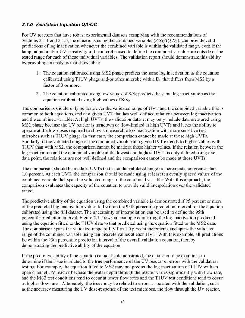
24

2.1.6 Validation Equation QA/QC

For UV reactors that have robust experimental datasets complying with the recommendations of Sections 2.1.1 and 2.1.5, the equations using the combined variable, (S/S0)/(Q DL), can provide valid predictions of log inactivation whenever the combined variable is within the validated range, even if the lamp output and/or UV sensitivity of the microbe used to define the combined variable are outside of the tested range for each of those individual variables. The validation report should demonstrate this ability by providing an analysis that shows that:

1. The equation calibrated using MS2 phage predicts the same log inactivation as the equation calibrated using T1UV phage and/or other microbe with a DL that differs from MS2 by a factor of 3 or more.

2. The equation calibrated using low values of S/S0 predicts the same log inactivation as the equation calibrated using high values of S/S0.

The comparisons should only be done over the validated range of UVT and the combined variable that is common to both equations, and at a given UVT that has well-defined relations between log inactivation and the combined variable. At high UVTs, the validation dataset may only include data measured using MS2 phage because the UV reactor is turndown or flow-limited at high UVTs and lacks the ability to operate at the low doses required to show a measurable log inactivation with more sensitive test microbes such as T1UV phage. In that case, the comparison cannot be made at those high UVTs. Similarly, if the validated range of the combined variable at a given UVT extends to higher values with T1UV than with MS2, the comparison cannot be made at those higher values. If the relation between the log inactivation and the combined variable at the lowest and highest UVTs is only defined using one data point, the relations are not well defined and the comparison cannot be made at those UVTs.

The comparison should be made at UVTs that span the validated range in increments not greater than 1.0 percent. At each UVT, the comparison should be made using at least ten evenly spaced values of the combined variable that span the validated range of the combined variable. With this approach, the comparison evaluates the capacity of the equation to provide valid interpolation over the validated range.

The predictive ability of the equation using the combined variable is demonstrated if 95 percent or more of the predicted log inactivation values fall within the 95th percentile prediction interval for the equation calibrated using the full dataset. The uncertainty of interpolation can be used to define the 95th percentile prediction interval. Figure 2.1 shows an example comparing the log inactivation predicted using the equation fitted to the T1UV data to that predicted using the equation fitted to the MS2 data. The comparison spans the validated range of UVT in 1.0 percent increments and spans the validated range of the combined variable using ten discrete values at each UVT. With this example, all predictions lie within the 95th percentile prediction interval of the overall validation equation, thereby demonstrating the predictive ability of the equation.

If the predictive ability of the equation cannot be demonstrated, the data should be examined to determine if the issue is related to the true performance of the UV reactor or errors with the validation testing. For example, the equation fitted to MS2 may not predict the log inactivation of T1UV with an open channel UV reactor because the water depth through the reactor varies significantly with flow rate, and the MS2 test conditions tend to occur at lower flow rates and the T1UV test conditions tend to occur as higher flow rates. Alternately, the issue may be related to errors associated with the validation, such as the accuracy measuring the UV dose-response of the test microbes, the flow through the UV reactor,

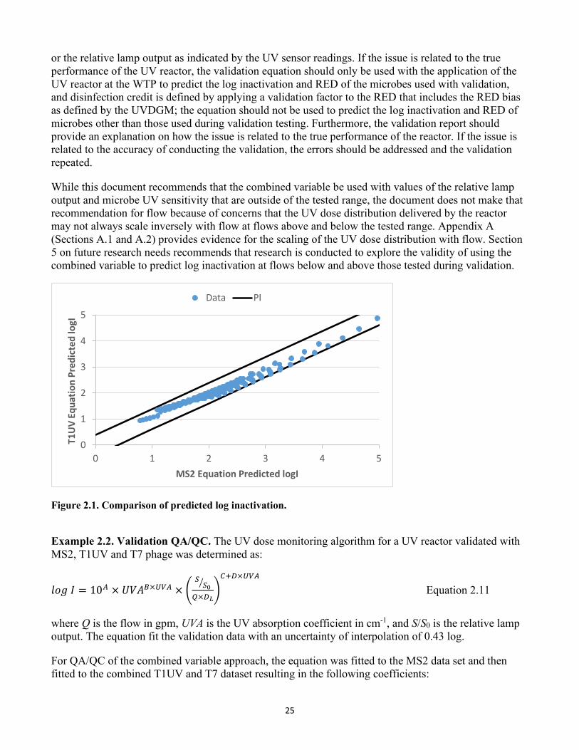
25

or the relative lamp output as indicated by the UV sensor readings. If the issue is related to the true performance of the UV reactor, the validation equation should only be used with the application of the UV reactor at the WTP to predict the log inactivation and RED of the microbes used with validation, and disinfection credit is defined by applying a validation factor to the RED that includes the RED bias as defined by the UVDGM; the equation should not be used to predict the log inactivation and RED of microbes other than those used during validation testing. Furthermore, the validation report should provide an explanation on how the issue is related to the true performance of the reactor. If the issue is related to the accuracy of conducting the validation, the errors should be addressed and the validation repeated.

While this document recommends that the combined variable be used with values of the relative lamp output and microbe UV sensitivity that are outside of the tested range, the document does not make that recommendation for flow because of concerns that the UV dose distribution delivered by the reactor may not always scale inversely with flow at flows above and below the tested range. Appendix A (Sections A.1 and A.2) provides evidence for the scaling of the UV dose distribution with flow. Section 5 on future research needs recommends that research is conducted to explore the validity of using the combined variable to predict log inactivation at flows below and above those tested during validation.

0

1

2

3

4

5

0 1 2 3 4 5

T1U

V Eq

uatio

n Pr

edic

ted

logI

MS2 Equation Predicted logI

Data PI

Figure 2.1. Comparison of predicted log inactivation.

Example 2.2. Validation QA/QC. The UV dose monitoring algorithm for a UV reactor validated with MS2, T1UV and T7 phage was determined as:


𝑄𝑄×𝑅𝑅𝐿𝐿�𝐶𝐶+𝑅𝑅×𝑈𝑈𝑈𝑈𝐴𝐴

Equation 2.11

where Q is the flow in gpm, UVA is the UV absorption coefficient in cm-1, and S/S0 is the relative lamp output. The equation fit the validation data with an uncertainty of interpolation of 0.43 log.

For QA/QC of the combined variable approach, the equation was fitted to the MS2 data set and then fitted to the combined T1UV and T7 dataset resulting in the following coefficients:

26

MS2 T1UV/T7

A 4.35 4.23

B 30.9 27.3

C 0.994 0.979

D -5.14 -3.51

Using the two sets of coefficients, the equation was used to calculate the log inactivation at UVTs and values of the combined variable that overlap. The log inactivation was calculated at UVTs ranging from 75 to 90 percent in 1 percent increments. At each UVT, log inactivation was calculated at ten values of the combined variable spanning the validated range of the combined variable at that UVT. Table 2.2 gives results at 80 and 81 percent UVT. Figure 2.2 shows that the results at 80 and 81 percent UVT lie within the 95th percentile prediction interval of the equation defined using the uncertainty of interpolation of 0.43 log.

Table 2.2: Comparison of log inactivation calculated using the validation equation fitted to the MS2 data to log inactivation calculated using the validation equation fitted to the combined T1UV and T7 data

UVT = 80 percent UVT = 81 percent Combined Variable

MS2 Equation log I

T1UV/T7 Equation log I

Combined Variable

MS2 Equation log I

T1UV/T7 Equation log I

0.001 0.67 0.43 0.001 0.70 0.46 0.005 1.49 1.20 0.005 1.62 1.32 0.01 2.10 1.86 0.01 2.32 2.09 0.014 2.49 2.31 0.014 2.77 2.61 0.019 2.89 2.81 0.018 3.16 3.07 0.023 3.18 3.17 0.023 3.59 3.61 0.028 3.50 3.60 0.027 3.91 4.01 0.032 3.74 3.92 0.031 4.20 4.40 0.037 4.02 4.30 0.036 4.54 4.85 0.041 4.23 4.59 0.04 4.80 5.20

Figure 2.2. Comparison of predicted log inactivation for example 2.2.

00.5

11.5

22.5

33.5

44.5

5

0 1 2 3 4 5

T1U

V/T7

Equ

atio

n lo

gI

MS2 Equation logI

27

2.1.7 Validated Range

If the predictive ability of the equation is demonstrated as per Section 2.1.6, the validated range can be defined using:

1. The minimum and maximum flow rates.

2. The minimum and maximum UVTs.

3. The minimum and maximum predicted log inactivation interpolated as a function of UVT using linear or cubic spline interpolation (examples in Figure 2.3 and Figure 2.4).

4. The minimum and maximum base 10 logarithm of the combined variable [i.e., log(CV)] interpolated as a function of UVT using linear or cubic spline interpolation (examples in Figure 2.5 and Figure 2.6).

5. If the equation includes a term for the number of banks of lamps, the minimum and maximum number of banks.

6. If the equation includes a term for the number of banks of lamps, the minimum and maximum predicted log inactivation interpolated as a function of the number of operating banks (example in Figure 2.9).

The validated limits of the predicted log inactivation and log(CV) are developed by connecting the validated test conditions to create a “validation envelope.” Additional details on the development of the validation envelopes for predicted log inactivation as a function of UVT, log(CV) as a function of UVT, and log inactivation as a function of banks are provided in the following sections.

2.1.7.1 Log Inactivation as a Function of UVT The minimum and maximum validated limits for the predicted log inactivation as a function of UVT should be developed using a minimum of three points, including:

1. Minimum validated UVT,

2. Maximum validated UVT, and

3. One or more intermediate UVT(s).

a. The minimum and maximum validated limits should be developed using a minimum of one intermediate UVT that falls within the 25th to 75th percentile of the validated UVT range (i.e. does not fall within the first or last quarter of the validated UVT range). For example, if a UV reactor is validated between 70 and 98 percent UVT, at least one intermediate UVT used to define the minimum validated limits should fall within 77 and 91 percent UVT.

b. The maximum validated limits should be developed from validation data where the maximum UVT spacing is no greater than 20 percent UVT units.

If the minimum predicted log inactivation interpolated as a function of UVT has a value of 1.0 or less, the validated range can be extended down to zero log inactivation.

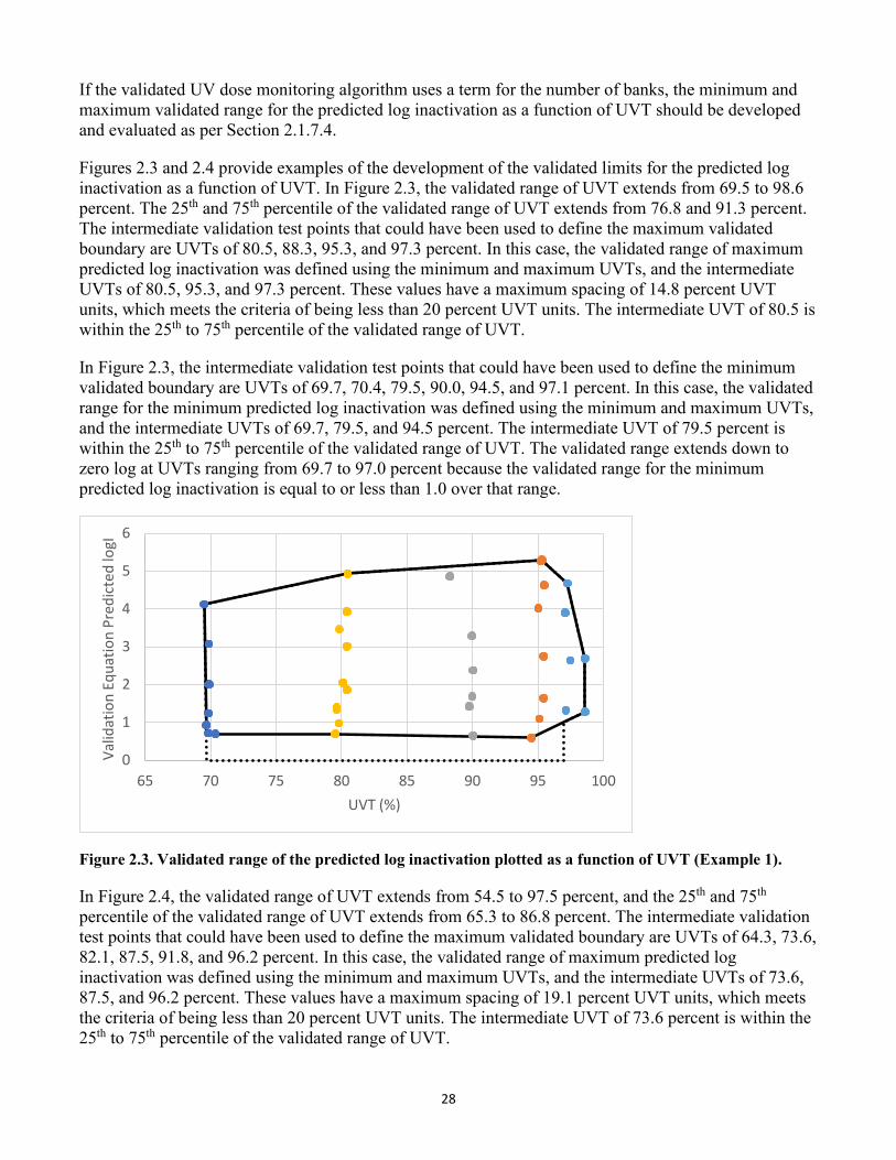
28

If the validated UV dose monitoring algorithm uses a term for the number of banks, the minimum and maximum validated range for the predicted log inactivation as a function of UVT should be developed and evaluated as per Section 2.1.7.4.

Figures 2.3 and 2.4 provide examples of the development of the validated limits for the predicted log inactivation as a function of UVT. In Figure 2.3, the validated range of UVT extends from 69.5 to 98.6 percent. The 25th and 75th percentile of the validated range of UVT extends from 76.8 and 91.3 percent. The intermediate validation test points that could have been used to define the maximum validated boundary are UVTs of 80.5, 88.3, 95.3, and 97.3 percent. In this case, the validated range of maximum predicted log inactivation was defined using the minimum and maximum UVTs, and the intermediate UVTs of 80.5, 95.3, and 97.3 percent. These values have a maximum spacing of 14.8 percent UVT units, which meets the criteria of being less than 20 percent UVT units. The intermediate UVT of 80.5 is within the 25th to 75th percentile of the validated range of UVT.

In Figure 2.3, the intermediate validation test points that could have been used to define the minimum validated boundary are UVTs of 69.7, 70.4, 79.5, 90.0, 94.5, and 97.1 percent. In this case, the validated range for the minimum predicted log inactivation was defined using the minimum and maximum UVTs, and the intermediate UVTs of 69.7, 79.5, and 94.5 percent. The intermediate UVT of 79.5 percent is within the 25th to 75th percentile of the validated range of UVT. The validated range extends down to zero log at UVTs ranging from 69.7 to 97.0 percent because the validated range for the minimum predicted log inactivation is equal to or less than 1.0 over that range.

Figure 2.3. Validated range of the predicted log inactivation plotted as a function of UVT (Example 1).

In Figure 2.4, the validated range of UVT extends from 54.5 to 97.5 percent, and the 25th and 75th percentile of the validated range of UVT extends from 65.3 to 86.8 percent. The intermediate validation test points that could have been used to define the maximum validated boundary are UVTs of 64.3, 73.6, 82.1, 87.5, 91.8, and 96.2 percent. In this case, the validated range of maximum predicted log inactivation was defined using the minimum and maximum UVTs, and the intermediate UVTs of 73.6, 87.5, and 96.2 percent. These values have a maximum spacing of 19.1 percent UVT units, which meets the criteria of being less than 20 percent UVT units. The intermediate UVT of 73.6 percent is within the 25th to 75th percentile of the validated range of UVT.

0

1

2

3

4

5

6

65 70 75 80 85 90 95 100

Valid

atio

n Eq

uatio

n Pr

edic

ted

logI

UVT (%)

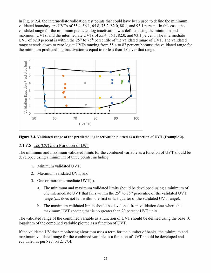
29

In Figure 2.4, the intermediate validation test points that could have been used to define the minimum validated boundary are UVTs of 55.4, 56.1, 65.8, 75.2, 82.0, 88.1, and 93.1 percent. In this case, the validated range for the minimum predicted log inactivation was defined using the minimum and maximum UVTs, and the intermediate UVTs of 55.4, 56.1, 82.0, and 93.1 percent. The intermediate UVT of 82.0 percent is within the 25th to 75th percentile of the validated range of UVT. The validated range extends down to zero log at UVTs ranging from 55.4 to 87 percent because the validated range for the minimum predicted log inactivation is equal to or less than 1.0 over that range.

0

1

2

3

4

5

6

7

50 60 70 80 90 100

Valid

atio

n Eq

uatio

n Pr

edic

ted

logI

UVT (%)

Figure 2.4. Validated range of the predicted log inactivation plotted as a function of UVT (Example 2).

2.1.7.2 Log(CV) as a Function of UVT The minimum and maximum validated limits for the combined variable as a function of UVT should be developed using a minimum of three points, including:

1. Minimum validated UVT,

2. Maximum validated UVT, and

3. One or more intermediate UVT(s).

a. The minimum and maximum validated limits should be developed using a minimum of one intermediate UVT that falls within the 25th to 75th percentile of the validated UVT range (i.e. does not fall within the first or last quarter of the validated UVT range).

b. The maximum validated limits should be developed from validation data where the maximum UVT spacing that is no greater than 20 percent UVT units.

The validated range of the combined variable as a function of UVT should be defined using the base 10 logarithm of the combined variable plotted as a function of UVT.

If the validated UV dose monitoring algorithm uses a term for the number of banks, the minimum and maximum validated range for the combined variable as a function of UVT should be developed and evaluated as per Section 2.1.7.4.

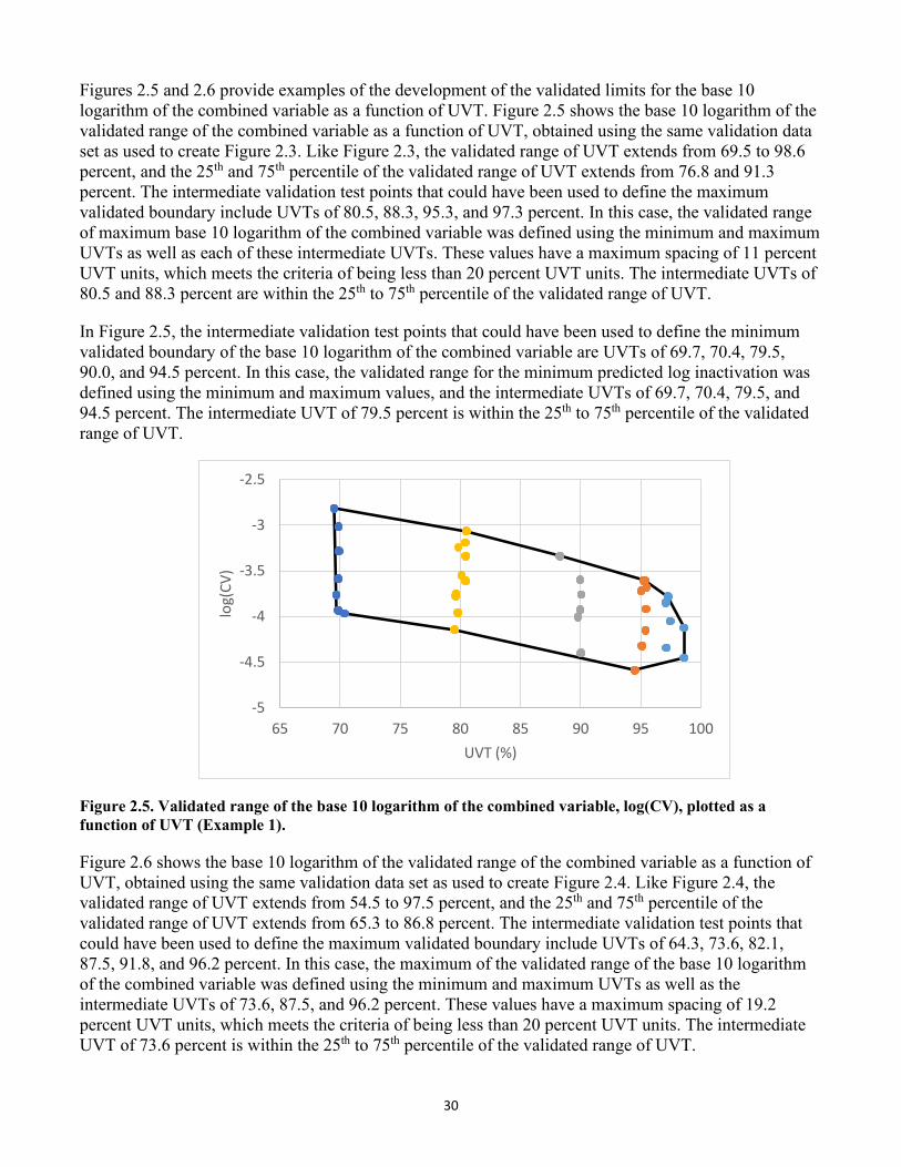
30

Figures 2.5 and 2.6 provide examples of the development of the validated limits for the base 10 logarithm of the combined variable as a function of UVT. Figure 2.5 shows the base 10 logarithm of the validated range of the combined variable as a function of UVT, obtained using the same validation data set as used to create Figure 2.3. Like Figure 2.3, the validated range of UVT extends from 69.5 to 98.6 percent, and the 25th and 75th percentile of the validated range of UVT extends from 76.8 and 91.3 percent. The intermediate validation test points that could have been used to define the maximum validated boundary include UVTs of 80.5, 88.3, 95.3, and 97.3 percent. In this case, the validated range of maximum base 10 logarithm of the combined variable was defined using the minimum and maximum UVTs as well as each of these intermediate UVTs. These values have a maximum spacing of 11 percent UVT units, which meets the criteria of being less than 20 percent UVT units. The intermediate UVTs of 80.5 and 88.3 percent are within the 25th to 75th percentile of the validated range of UVT.

In Figure 2.5, the intermediate validation test points that could have been used to define the minimum validated boundary of the base 10 logarithm of the combined variable are UVTs of 69.7, 70.4, 79.5, 90.0, and 94.5 percent. In this case, the validated range for the minimum predicted log inactivation was defined using the minimum and maximum values, and the intermediate UVTs of 69.7, 70.4, 79.5, and 94.5 percent. The intermediate UVT of 79.5 percent is within the 25th to 75th percentile of the validated range of UVT.

-5

-4.5

-4

-3.5

-3

-2.5

65 70 75 80 85 90 95 100

log(

CV)

UVT (%)

Figure 2.5. Validated range of the base 10 logarithm of the combined variable, log(CV), plotted as a function of UVT (Example 1).

Figure 2.6 shows the base 10 logarithm of the validated range of the combined variable as a function of UVT, obtained using the same validation data set as used to create Figure 2.4. Like Figure 2.4, the validated range of UVT extends from 54.5 to 97.5 percent, and the 25th and 75th percentile of the validated range of UVT extends from 65.3 to 86.8 percent. The intermediate validation test points that could have been used to define the maximum validated boundary include UVTs of 64.3, 73.6, 82.1, 87.5, 91.8, and 96.2 percent. In this case, the maximum of the validated range of the base 10 logarithm of the combined variable was defined using the minimum and maximum UVTs as well as the intermediate UVTs of 73.6, 87.5, and 96.2 percent. These values have a maximum spacing of 19.2 percent UVT units, which meets the criteria of being less than 20 percent UVT units. The intermediate UVT of 73.6 percent is within the 25th to 75th percentile of the validated range of UVT.

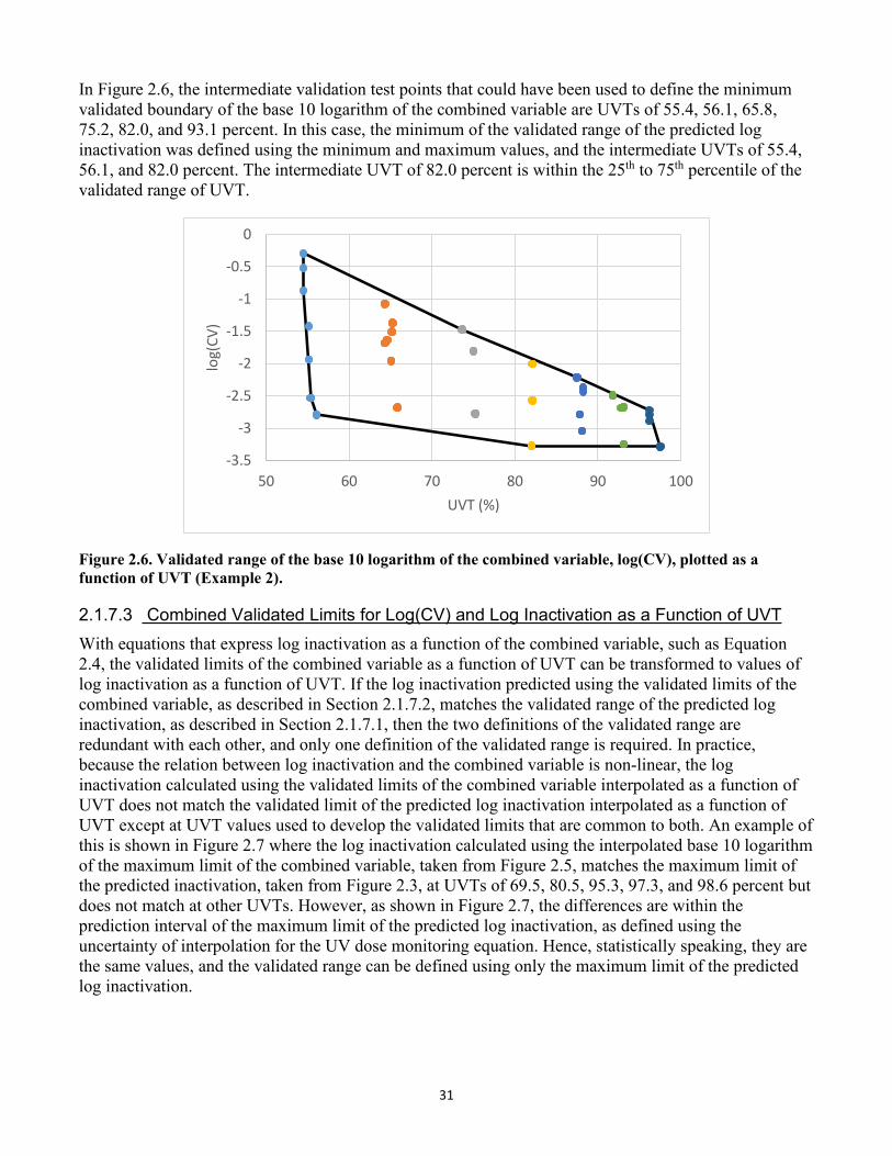
31

In Figure 2.6, the intermediate validation test points that could have been used to define the minimum validated boundary of the base 10 logarithm of the combined variable are UVTs of 55.4, 56.1, 65.8, 75.2, 82.0, and 93.1 percent. In this case, the minimum of the validated range of the predicted log inactivation was defined using the minimum and maximum values, and the intermediate UVTs of 55.4, 56.1, and 82.0 percent. The intermediate UVT of 82.0 percent is within the 25th to 75th percentile of the validated range of UVT.

-3.5

-3

-2.5

-2

-1.5

-1

-0.5

0

50 60 70 80 90 100

log(

CV)

UVT (%)

Figure 2.6. Validated range of the base 10 logarithm of the combined variable, log(CV), plotted as a function of UVT (Example 2).

2.1.7.3 Combined Validated Limits for Log(CV) and Log Inactivation as a Function of UVT With equations that express log inactivation as a function of the combined variable, such as Equation 2.4, the validated limits of the combined variable as a function of UVT can be transformed to values of log inactivation as a function of UVT. If the log inactivation predicted using the validated limits of the combined variable, as described in Section 2.1.7.2, matches the validated range of the predicted log inactivation, as described in Section 2.1.7.1, then the two definitions of the validated range are redundant with each other, and only one definition of the validated range is required. In practice, because the relation between log inactivation and the combined variable is non-linear, the log inactivation calculated using the validated limits of the combined variable interpolated as a function of UVT does not match the validated limit of the predicted log inactivation interpolated as a function of UVT except at UVT values used to develop the validated limits that are common to both. An example of this is shown in Figure 2.7 where the log inactivation calculated using the interpolated base 10 logarithm of the maximum limit of the combined variable, taken from Figure 2.5, matches the maximum limit of the predicted inactivation, taken from Figure 2.3, at UVTs of 69.5, 80.5, 95.3, 97.3, and 98.6 percent but does not match at other UVTs. However, as shown in Figure 2.7, the differences are within the prediction interval of the maximum limit of the predicted log inactivation, as defined using the uncertainty of interpolation for the UV dose monitoring equation. Hence, statistically speaking, they are the same values, and the validated range can be defined using only the maximum limit of the predicted log inactivation.

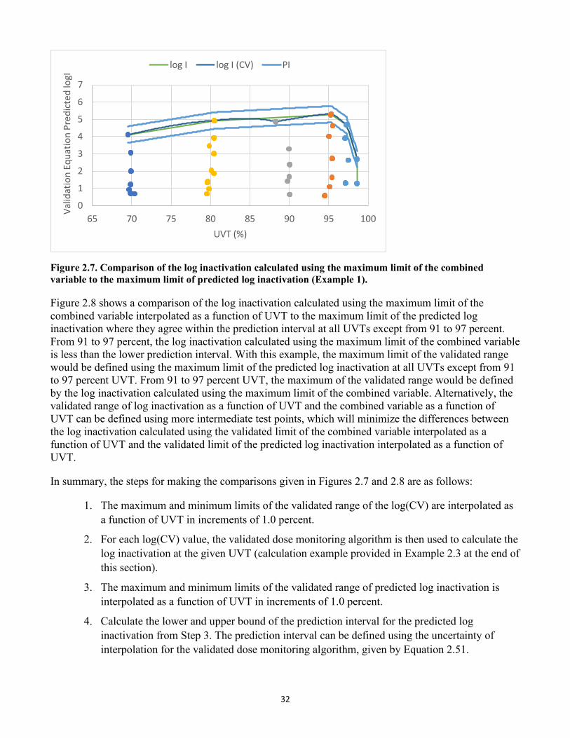
32

0

1

2

3

4

5

6

7

65 70 75 80 85 90 95 100

Valid

atio

n Eq

uatio

n Pr

edic

ted

logI

UVT (%)

log I log I (CV) PI

Figure 2.7. Comparison of the log inactivation calculated using the maximum limit of the combined variable to the maximum limit of predicted log inactivation (Example 1).

Figure 2.8 shows a comparison of the log inactivation calculated using the maximum limit of the combined variable interpolated as a function of UVT to the maximum limit of the predicted log inactivation where they agree within the prediction interval at all UVTs except from 91 to 97 percent. From 91 to 97 percent, the log inactivation calculated using the maximum limit of the combined variable is less than the lower prediction interval. With this example, the maximum limit of the validated range would be defined using the maximum limit of the predicted log inactivation at all UVTs except from 91 to 97 percent UVT. From 91 to 97 percent UVT, the maximum of the validated range would be defined by the log inactivation calculated using the maximum limit of the combined variable. Alternatively, the validated range of log inactivation as a function of UVT and the combined variable as a function of UVT can be defined using more intermediate test points, which will minimize the differences between the log inactivation calculated using the validated limit of the combined variable interpolated as a function of UVT and the validated limit of the predicted log inactivation interpolated as a function of UVT.

In summary, the steps for making the comparisons given in Figures 2.7 and 2.8 are as follows:

1. The maximum and minimum limits of the validated range of the log(CV) are interpolated as a function of UVT in increments of 1.0 percent.

2. For each log(CV) value, the validated dose monitoring algorithm is then used to calculate the log inactivation at the given UVT (calculation example provided in Example 2.3 at the end of this section).

3. The maximum and minimum limits of the validated range of predicted log inactivation is interpolated as a function of UVT in increments of 1.0 percent.

4. Calculate the lower and upper bound of the prediction interval for the predicted log inactivation from Step 3. The prediction interval can be defined using the uncertainty of interpolation for the validated dose monitoring algorithm, given by Equation 2.51.

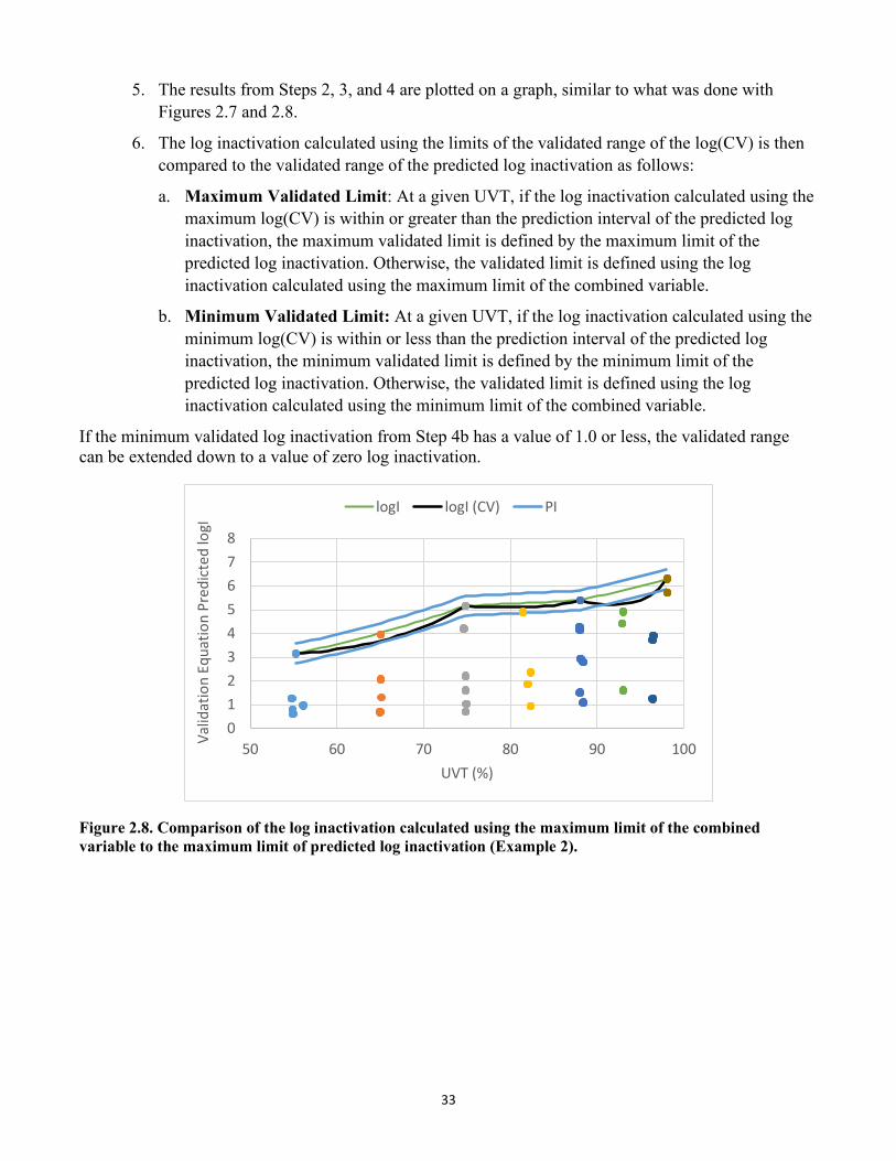
33

5. The results from Steps 2, 3, and 4 are plotted on a graph, similar to what was done with Figures 2.7 and 2.8.

6. The log inactivation calculated using the limits of the validated range of the log(CV) is then compared to the validated range of the predicted log inactivation as follows:

a. Maximum Validated Limit: At a given UVT, if the log inactivation calculated using the maximum log(CV) is within or greater than the prediction interval of the predicted log inactivation, the maximum validated limit is defined by the maximum limit of the predicted log inactivation. Otherwise, the validated limit is defined using the log inactivation calculated using the maximum limit of the combined variable.

b. Minimum Validated Limit: At a given UVT, if the log inactivation calculated using the minimum log(CV) is within or less than the prediction interval of the predicted log inactivation, the minimum validated limit is defined by the minimum limit of the predicted log inactivation. Otherwise, the validated limit is defined using the log inactivation calculated using the minimum limit of the combined variable.

If the minimum validated log inactivation from Step 4b has a value of 1.0 or less, the validated range can be extended down to a value of zero log inactivation.

012345678

50 60 70 80 90 100Valid

atio

n Eq

uatio

n Pr

edic

ted

logI

UVT (%)

logI logI (CV) PI

Figure 2.8. Comparison of the log inactivation calculated using the maximum limit of the combined variable to the maximum limit of predicted log inactivation (Example 2).

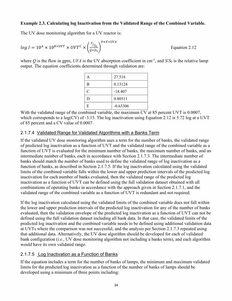
34

Example 2.3. Calculating log Inactivation from the Validated Range of the Combined Variable.

The UV dose monitoring algorithm for a UV reactor is:

𝑉𝑉𝐷𝐷𝑙𝑙 𝐼𝐼 = 10𝐴𝐴 × 10𝐵𝐵×𝑈𝑈𝑈𝑈𝑈𝑈 × 𝑈𝑈𝑉𝑉𝑈𝑈𝐶𝐶 × �𝑆𝑆𝑆𝑆0�

𝑄𝑄×𝑅𝑅𝐿𝐿�𝑅𝑅+𝑅𝑅×𝑈𝑈𝑈𝑈𝐴𝐴

Equation 2.12

where Q is the flow in gpm, UVA is the UV absorption coefficient in cm-1, and S/S0 is the relative lamp output. The equation coefficients determined through validation are:

A 27.516

B 0.13124

C -18.407

D 0.80511

E -0.63306 With the validated range of the combined variable, the maximum CV at 85 percent UVT is 0.0007, which corresponds to a log(CV) of -3.15. The log inactivation using Equation 2.12 is 5.72 log at a UVT of 85 percent and a CV value of 0.0007.

2.1.7.4 Validated Range for Validated Algorithms with a Banks Term If the validated UV dose monitoring algorithm uses a term for the number of banks, the validated range of predicted log inactivation as a function of UVT and the validated range of the combined variable as a function of UVT is evaluated for the minimum number of banks, the maximum number of banks, and an intermediate number of banks, each in accordance with Section 2.1.7.3. The intermediate number of banks should match the number of banks used to define the validated range of log inactivation as a function of banks, as described in Section 2.1.7.5. If the log inactivation calculated using the validated limits of the combined variable falls within the lower and upper prediction intervals of the predicted log inactivation for each number of banks evaluated, then the validated range of the predicted log inactivation as a function of UVT can be defined using the full validation dataset obtained with all combinations of operating banks in accordance with the approach given in Section 2.1.7.1, and the validated range of the combined variable as a function of UVT is redundant and not required.

If the log inactivation calculated using the validated limits of the combined variable does not fall within the lower and upper prediction intervals of the predicted log inactivation for any of the number of banks evaluated, then the validation envelope of the predicted log inactivation as a function of UVT can not be defined using the full validation dataset including all bank data. In that case, the validated limits of the predicted log inactivation and the combined variable needs to be defined using additional validation data at UVTs where the comparison was not successful, and the analysis per Section 2.1.7.3 repeated using that additional data. Alternatively, the UV dose algorithm should be developed for each of validated bank configuration (i.e., UV dose monitoring algorithm not including a banks term), and each algorithm would have its own validated range.

2.1.7.5 Log Inactivation as a Function of Banks If the equation includes a term for the number of banks of lamps, the minimum and maximum validated limits for the predicted log inactivation as a function of the number of banks of lamps should be developed using a minimum of three points including:

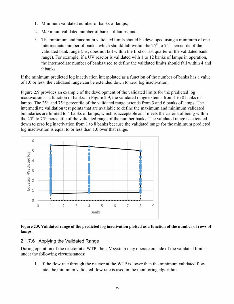
35

1. Minimum validated number of banks of lamps,

2. Maximum validated number of banks of lamps, and

3. The minimum and maximum validated limits should be developed using a minimum of one intermediate number of banks, which should fall within the 25th to 75th percentile of the validated bank range (i.e., does not fall within the first or last quarter of the validated bank range). For example, if a UV reactor is validated with 1 to 12 banks of lamps in operation, the intermediate number of banks used to define the validated limits should fall within 4 and 9 banks.

If the minimum predicted log inactivation interpolated as a function of the number of banks has a value of 1.0 or less, the validated range can be extended down to zero log inactivation.

Figure 2.9 provides an example of the development of the validated limits for the predicted log inactivation as a function of banks. In Figure 2.9, the validated range extends from 1 to 8 banks of lamps. The 25th and 75th percentile of the validated range extends from 3 and 6 banks of lamps. The intermediate validation test points that are available to define the maximum and minimum validated boundaries are limited to 4 banks of lamps, which is acceptable as it meets the criteria of being within the 25th to 75th percentile of the validated range of the number banks. The validated range is extended down to zero log inactivation from 1 to 8 banks because the validated range for the minimum predicted log inactivation is equal to or less than 1.0 over that range.

0

1

2

3

4

5

6

0 1 2 3 4 5 6 7 8 9

Equa

tion-

Pred

icte

d lo

gI

Banks

Figure 2.9. Validated range of the predicted log inactivation plotted as a function of the number of rows of lamps.

2.1.7.6 Applying the Validated Range During operation of the reactor at a WTP, the UV system may operate outside of the validated limits under the following circumstances:

1. If the flow rate through the reactor at the WTP is lower than the minimum validated flow rate, the minimum validated flow rate is used in the monitoring algorithm.

36

2. If the UVT at the WTP is greater than the maximum validated UVT, the maximum validated UVT is used in the monitoring algorithm.

3. If the number of operating banks at the WTP is greater than the maximum validated number of banks, the maximum validated number of banks is used in the monitoring algorithm.

4. If the predicted log inactivation at the WTP is greater than the maximum limit of the validated range, the maximum validated log inactivation should be used for calculating inactivation credit by the reactor.

5. If the maximum validated base 10 logarithm of the combined variable, log(CV), defined as a function of UVT, is used to define the validated range, and if the log(CV) at the WTP is greater than the maximum validated log(CV), the maximum validated log(CV) is used in the monitoring algorithm.

6. There may be situations where the minimum predicted log inactivation at a given UVT is greater than 1.0 log and the minimum validated range does not extend to zero log inactivation (e.g., Figure 2.4 above 87 percent UVT). This often occurs at high UVTs because the reactor is turndown or flow-limited and lacks the ability to operate at the low doses required to show low log inactivation. If this situation occurs, the log inactivation can be linearly interpolated down to zero from the minimum predicted log inactivation. This approach provides a conservative prediction of log inactivation because the relation between log inactivation and the combined variable is always concave downward (i.e., the slope decreases with higher values of the combined variable), as shown in Figure A.7.

With these approaches, the monitoring algorithm will provide a conservative estimate of the log inactivation and RED achieved by the UV reactor.

The UV reactor is off-spec if:

1. The flow is greater than the maximum validated flow.

2. The UVT is lower than the minimum validated UVT.

3. The number of operating banks of lamps is lower than the minimum validated number of banks.

4. If the predicted log inactivation is lower than the minimum limit of the validated range. Alternately, the log inactivation can be linearly interpolated down to zero from the minimum predicted log inactivation as described in item (6) listed above.

5. If the minimum validated base 10 logarithm of the combined variable, log(CV), defined as a function of UVT, is used to define the validated range, and if the CV is less than the minimum validated CV. Alternatively, the log inactivation calculated using the minimum validated CV can be linearly interpolated down to zero as described in item (6) listed above.

6. The validated UV dose is less than the required UV dose.

7. The reactor is operating with a non-validated configuration of lamps.

8. The reactor is operating with UV sensors or an on-line UVT monitor that is not in compliance with the calibration requirements of Section 6.4.1.1 and Section 6.4.1.2 of the UVDGM, respectively.

37

9. The reactor is operating with UV sensors that are reading below their working range, and potentially providing a non-linear response.

As shown in Figure 2.3, the validated range of predicted log inactivation extends to higher log inactivation values at a UVT of 95 percent than at UVTs greater than 95 percent. If the reactor was operating at UVTs greater than 95 percent, it would be acceptable to set UVT to 95 percent with the monitoring algorithm to allow for predictions at those higher log inactivations.

While this report provides detailed approaches for the development of the validated range, future research may support the application of alternative approaches. Chapter 5 of this document describes future research needs, including 1) the use of the combined variable at flows below and above the validated range, and 2) using bank additivity to predict the performance of a UV reactor with banks in series that is operated with a greater number of banks than were validated. CFD-based UV dose models are a powerful tool that can be used to evaluate both of these scenarios. For example, Section A.2 provides two approaches for showing that the UV dose distributions delivered by a UV reactor scale inversely with flow. CFD-based UV dose models can also be used to evaluate bank additivity. With both of these approaches, the CFD-based UV dose models should be proven by the comparison with validation data, in accordance with the recommendations of Linden et al. (2015).

2.1.8 Validation Report

The validation report should include the following sections:

1. Executive Summary - includes the UV sensor and UV dose monitoring equations, validated range, validation factors, and required REDs for disinfection credit, compliance to UVDGM checklists, and description of any significant deviations and performance implications.

2. UV Reactor Documentation - describes the wetted dimensions of the reactor and optical properties of the lamps, sleeves, UV sensors, and UV sensor ports that impact UV dose delivery and monitoring.

3. Validation Methods – includes:

a. Description of the test train.

b. UV reactor inlet and outlet piping with dimensions.

c. Challenge microorganism stock solution preparation.

d. Challenge microorganism enumeration.

e. Third party oversight as defined in Section 5.2.3 of the UVDGM.

f. Water quality measurement methods (UVT, chlorine, etc.).

g. Functional test methods (head loss, power, UV sensor reference checks, and UV sensor equation development).

h. Biodosimetry methods.

i. QA/QC (Accuracy of instrumentation, microbial, lamp output, mixing, etc.).

4. Validation Results – includes:

a. Water quality measurements (e.g., UVT, chlorine, temperature, etc.).

38

b. Head loss vs. flow curves.

c. Lamp output ranking and positioning if the number of UV sensors is less than the number of lamps.

d. Power consumption vs. power setting curves.

e. Results of duty UV sensor checks using reference UV sensors.

f. Analysis describing development of UV sensor equations with tabulated coefficients and plots of measured vs. predicted UV sensor readings.

g. Challenge microorganism UV dose response curves with fits and QA/QC bounds.

h. Analysis describing development of UV dose monitoring algorithm with tabulated coefficients and plots of measured vs. predicted log inactivation and RED.

i. Analysis and plots showing that MS2 predicts T1UV and vice versa.

j. Plots and tabulated data showing the validated range, and any analysis that shows the validated range of the combined variable as a function of UVT is not required.

k. Example calculations using UV dose monitoring algorithms.

5. Validation Factor Analysis – includes:

a. RED bias.

b. Polychromatic bias, if applicable.

c. Uncertainty of validation.

d. Tables showing validation factors and required REDs for disinfection credit.

6. Compliance to UVDGM Checklists, and descriptions of deviations and potential performance and operational implications.

7. Appendices, including:

a. Functional and biodosimetric data.

b. QA/QC results (microbial, UVT monitors, mixing, etc.).

c. Calibration certificates for UV sensors, UVT monitors, flowmeters, radiometers, and power meters.

d. Microbial methods.

2.2 Calculated Dose Approach Using a Combined Variable and No UVT Monitor

This section describes the validation and application of a calculated dose approach that predicts log inactivation and RED as a function of the flow rate through the reactor, UV sensor readings, and the UV dose per log inactivation of the microbe whose log inactivation is predicted. This approach does not require UVT as an input to the monitoring algorithm.

As described in Appendix A, CFD-based UV dose models and validation data with UV reactors using monochromatic LP or LPHO lamps show that log inactivation by a UV reactor operating with a given number of lamps at a fixed UVT lies along a single relationship defined as a function of the combined

39

variable, S/(Q DL). If the UV sensor is optimally positioned, the relationships between the log inactivation and the combined variable at different UVTs tend to align on top of each other. If this is the case, a single relationship between log inactivation and the combined variable can be used for efficient UV dose monitoring that does not require an online UVT monitor (see Section A.5 for more detail on this approach).

This approach can be used with UV systems equipped with LP or LPHO lamps as well as UV systems equipped with MP UV lamps and monitoring by a UV sensor with a high wavelength UV sensor as defined by Section 5.4.8 of the UVDGM. With UV systems equipped with MP lamps, the validation factor would need to include an ASCF value calculated in accordance with the recommendations of Linden et al. (2015), as described in Section 3.5 of this document. Existing validation datasets can be re-analyzed using this approach if they meet the recommendations of this section. If needed, UV sensor data can be measured at different water layer distances from the UV sensor to the lamp, as detailed in Section 2.2.2, to support the re-analysis.

2.2.1 Test Plan

The test plan is the same as outlined in Section 2.1.1 with the additional requirement that the relationships between log inactivation and the combined variable [S/(Q DL)] should be evaluated over at least four UVT values. The four UVT values provide sufficient information to define the optimal UV sensor location, as will be described in the analysis section for this approach.

2.2.2 Functional Testing

The functional testing is the same as outlined in Section 2.1.2 with the additional requirement that the dependence of the UV sensor reading on UVT and lamp power settings should be measured at four or more distinct water layer distances. To achieve this, the UV reactor is equipped with a UV sensor port with an adjustable water layer distance between the UV sensor port window and the UV lamp. The water layer distance is adjusted by moving the UV sensor port closer or farther from the lamp. The movable UV sensor port should have a means of accurately measuring the distance from the UV sensor port window to the quartz sleeve housing of the lamp.

The UV reactor would not be implemented at the PWS with an adjustable water layer distance. Instead, the water layer distance would be fixed at the optimal location as determined in Section 2.2.5.

2.2.3 Analysis of UV Sensor Data

At each water layer distance, an equation that predicts the UV sensor readings as a function of UVT and ballast power setting should be identified. As an example, the measured UV sensor readings at each water layer may be well-modeled using:

𝑆𝑆 = 10𝑎𝑎′ × 𝑃𝑃𝑏𝑏′ × 𝑡𝑡𝑒𝑒𝑒𝑒(𝑐𝑐′ × 𝑈𝑈𝑉𝑉𝑈𝑈) Equation 2.13

where S is the UV sensor reading, P is the ballast power setting, UVT is the UVT at 254 nm, and a', b' and c' are coefficients determined by fitting the equation using regression analysis to the UV sensor data. Ideally, the equation can be linearized by taking the log transform and the coefficients can be determined using linear regression. If the equation cannot be linearized, the coefficients can be determined using non-linear regression. In that case, the regression analysis should minimize the sum of the squares of the percent differences between the measured and predicted UV sensor readings, as opposed to the absolute differences. This ensures that the fit provides a similar relative accuracy

40

predicting the UV sensor reading over the full working range of the UV sensor, which may extend for more than one order of magnitude. The coefficients with the UV sensor equation should be statistically significant at a 95th percent confidence level (i.e., p-stat < 0.05).

The equation used to model the UV sensor readings with each water layer should have the same functional relationships and the same number of coefficients. Model the dependence of the coefficients of the UV sensor equation on the water layer. For example, the coefficients of Equation 2.13 could be modeled using quadratic equations:

𝑉𝑉′ = 𝑉𝑉1′ + 𝑉𝑉2′ × 𝑤𝑤𝑉𝑉 + 𝑉𝑉3′ × 𝑤𝑤𝑉𝑉2 Equation 2.14

𝑏𝑏′ = 𝑏𝑏1′ + 𝑏𝑏2′ × 𝑤𝑤𝑉𝑉 + 𝑏𝑏3′ × 𝑤𝑤𝑉𝑉2 Equation 2.15

𝑐𝑐′ = 𝑐𝑐1′ + 𝑐𝑐2′ × 𝑤𝑤𝑉𝑉 + 𝑐𝑐3′ × 𝑤𝑤𝑉𝑉2 Equation 2.16

where wl is the water layer distance and a'1 to a'3, b'1 to b'3, and c'1 to c'3 are constants determined using regression analysis. Use non-linear regression to further refine the coefficients that predict the dependence of UV sensor readings on the water layer. The non-linear regression should minimize the sum of squares of the percent differences between the measured and predicted UV sensor readings, as opposed to the absolute differences.

The quality of the equation predicting the UV sensor readings as a function of UVT, ballast power setting, and water layer should be evaluated by plotting the measured UV sensor readings as a function of the predicted UV sensor readings. The slope should be within 5 percent of a one-to-one relationship and the R-squared value should be above 0.98.

Appendix B (Section B.3.1) provides an example where a UV sensor equation was developed that predicts UV sensor readings as a function of UVT, lamp power, and water layer.


Biodosimetric testing should be conducted in accordance with the validation protocol of the UVDGM. During testing, it is recommended that the UV sensor is located at an intermediate water layer distance. With many UV reactors, the water layer distance used by the UV sensor has a small impact on the flow patterns in the reactor, and as such, a minor impact on the log inactivation. If needed, CFD-based UV dose models or biodosimetric testing can be conducted to show that the UV sensor water layer can be adjusted without a significant impact on log inactivation by the reactor (i.e., the impact is within the uncertainty of interpolation calculated per Equation 2.51).

2.2.5 Analysis of Biodosimetric Data

The analysis of the biodosimetry data should identify the optimum location for the UV sensors and result in a UV dose monitoring algorithm that does not require UVT as an input. This begins by analyzing the biodosimetry data as outlined in Section 2.1.5 to develop an equation that predicts log inactivation as a function of UVT and the combined variable (S/S0)/(Q DL).

To identify the optimal UV sensor location, the equation derived from analyzing the biodosimetry data is used to predict log inactivation as a function of the combined variable (S/S0)/(Q DL) at a minimum of

41

six discrete UVTs that span the tested range.7 For example, if the UV reactor was tested at UVTs ranging from 85 to 98 percent, the equation would be used to predict log inactivation at UVTs of 85, 88, 91, 94, 96, and 98 percent. The values of (S/S0)/(Q DL) should be selected to span the validated range of (S/S0)/(Q DL) at each UVT, as defined in Section 2.1.7.2. The UV sensor equation, derived from analyzing the functional test data as outlined in Section 2.2.3, is then used to predict the UV sensor readings at different water layers, which in turn are used to calculate values of S/(Q DL) associated with each predicted value of log inactivation. The optimal water layer is then identified as the UV sensor position where the relationships between log inactivation and the combined variable S/(Q DL) at different UVTs tend to line up with each other. Figures A.30 and A.31 of Appendix A show examples of this approach.

If the UV reactor delivers a narrow UV dose distribution, the relations between log inactivation and the combined variable at a given UVT will be linear. If the UV reactor delivers a wide UV dose distribution, the relations between log inactivation and the combined variable will show curvature (e.g., Figure A.7). That curvature becomes more pronounced with a wider UV dose distribution which tends to occur at lower UVT values. If the relations at different UVTs have different curvature, one cannot identify a water layer where those relations will exactly lie on top of each other. Hence, at the "ideal" UV sensor location, at a given value of the combined variable S/(Q DL), the relations at some UVT will give the lowest log inactivation. In many cases, a plot of log inactivation as a function of UVT at a given value of the combined variable S/(Q DL) is parabolic with a minimum value of log inactivation at an intermediate UVT. If an intermediate UVT is used to define the lowest log inactivation, then a UVT monitor is not required because UVTs lower and higher than that intermediate UVT will give higher values of log inactivation with a given value of the combined variable, S/(Q DL).

With the water layer that gives the best overlap of the relations between log inactivation and the combined variable S/(Q DL), the minimum log inactivation as a function of the combined variable S/(Q DL) should be identified. The relation between the minimum log inactivation and the combined variable should be fitted to define the monitoring algorithm. For example, the relation may be fitted by a quadratic function:

𝑉𝑉𝐷𝐷𝑙𝑙 𝐼𝐼 = 𝐴𝐴" × � 𝑆𝑆𝑄𝑄×𝑅𝑅𝐿𝐿

� + 𝐵𝐵" × � 𝑆𝑆𝑄𝑄×𝑅𝑅𝐿𝐿

�2 Equation 2.17

where A" and B" are coefficients obtained by fitting the equation to the minimum log inactivation as a function of the combined variable, S/(Q DL). With this approach, the manufacturer may wish to define algorithms for different water layers where one algorithm provides more efficient sizing and operation for high UVT applications while a second algorithm provides more efficient sizing and operation for low UVT applications.

7 While the test plan may evaluate log inactivation at four UVTs, the equation developed using the validation data can predict log inactivation at multiple UVTs, which is recommended to identify the optimal UV sensor location.

42

The algorithm can also be developed specific for a target pathogen by setting the value of DL to that of the target pathogen during the analysis and incorporating the validation factor. In that case, the equation could be defined as:

𝑉𝑉𝐷𝐷𝑙𝑙 𝐼𝐼 = 𝐴𝐴" × �𝑆𝑆𝑄𝑄�+ 𝐵𝐵" × �𝑆𝑆

𝑄𝑄�2 Equation 2.18

or

𝐷𝐷𝑈𝑈𝑎𝑎𝑃𝑃 = 𝐴𝐴" × �𝑆𝑆𝑄𝑄� + 𝐵𝐵" × �𝑆𝑆

𝑄𝑄� 2

Equation 2.19

where log I is the pathogen inactivation credit and Dval is the validated dose. With this analysis, the optimum location with Equation 2.18 is identified by plotting log inactivation as a function of S/Q and the optimum location with Equation 2.19 is identified by plotting Dval as a function of S/Q. The values of DL for the pathogen would be calculated by interpolating the UV dose requirements defined by the LT2ESWTR, as described in Sections 2.7 and 2.8. As such, the values of DL will vary depending on the predicted log inactivation. The validation factor would be calculated per the UVDGM as described in Section 2.6. ASCF values would be incorporated into the analysis with MP systems, as defined in Section 3.6. The main benefit of incorporating the value of DL and the validation factor into the UV dose monitoring equation is that it simplifies the programing of the UV reactor's programmable logic controller (PLC); the PLC does not need to calculate the values of DL and the validation factor.


The equation using the combined variable, S/(Q DL), can provide valid predictions of log inactivation whenever the combined variable is within the validated range, even if the UV dose per log inactivation (DL) used to define the combined variable is outside of the tested range. As described in Section 2.1.6, the validation report should demonstrate this ability by providing an analysis that shows that the equation developed per Section 2.1.5 when calibrated using MS2 phage, predicts T1UV log inactivation, and vice versa.

If the predictive capacity of the equation is demonstrated, the validated range for the equation developed per Section 2.2.5 can be defined using:

1. The minimum and maximum validated flow rates.

2. The minimum and maximum predicted log inactivation in the case of Equation 2.17 or 2.18 or the minimum and maximum predicted validated dose in the case of Equation 2.19. The validated range of log inactivation or validated dose can be extended to zero if the minimum predicted log inactivation is equal to or less than 1.0.

With this combined variable approach, during operation of the reactor at a WTP, the UV system may operate outside of the validated limits under the following circumstances:

1. If the flow is less than the minimum validated flow, the minimum validated flow is used in the monitoring algorithm.

2. If the predicted log inactivation is greater than the maximum predicted log inactivation or the predicted validated dose is greater than the maximum validated dose, the maximum value should be used for defining the inactivation credit by the reactor.

43




2. If the predicted log inactivation or validated dose is less than the validated range of those values.

3. The UV dose is less than the required UV dose


5. The reactor is operating with UV sensors that are not in compliance with the calibration requirements of Section 6.4.1.1 of the UVDGM.

6. The reactor is operating with UV sensors that are reading below their working range, and potentially providing a non-linear response.

If the water layer is selected such that an intermediate UVT defines the minimum log inactivation, then the algorithm will provide valid predictions of log inactivation at lower and higher UVTs, even if those UVTs were not evaluated during biodosimetric testing. However, if the water layer is selected such that the minimum tested UVT defines the minimum log inactivation, one cannot say if a lower UVT would have given a lower log inactivation. In that case, reactor performance would be treated as off-spec if the UVT dropped below that minimum tested UVT. In a similar way, if the water layer is selected such that the maximum tested UVT defines the minimum log inactivation, one cannot say if a higher UVT would have given a lower low inactivation. In that case, reactor performance would be treated as off-spec if the UVT was greater than that maximum tested UVT. For these reasons, a UV dose monitoring algorithm that does not require a UVT monitor should use a water layer where the intermediate UVT defines the lowest log inactivation.


The validation report should include the sections described in Section 2.1.8, as well as:

1. A description how the water layer distance was adjusted during functional testing.

2. Functional test data giving UV sensor readings as a function of water layer, UVT, and lamp power.

3. An analysis showing the development of the equation predicting UV sensor readings as a function of the water layer distance. The plot of measured versus predicted UV sensor readings should be based on the final equation that includes a term for the water layer.

4. Plots showing log inactivation or validated dose as a function of the combined variable [S/(Q DL) or S/Q] at the optimal position. The plot should include the final relationship predicting log inactivation as a function of the combined variable (e.g., Equations 2.17, 2.18, or 2.19).

5. If the dependence of the UV sensor readings on the water layer distance was determined for a UV reactor with a pre-existing validation dataset, the analysis should address any differences in the lamp output observed with the original UV validation and with the evaluation of the dependence of UV sensor readings on the water layer.

44

2.3 Calculated Dose Approach with Low and High Wavelength UV Sensors and UVT Monitors

This section describes the validation and application of a calculated dose approach for UV systems using MP lamps that predicts log inactivation and RED as the sum contribution of the log inactivations achieved by wavelengths below and above 240 nm. The high wavelength component of log inactivation is predicted as a function of the flow rate through the reactor, the UVT of the water at 254 nm, the high wavelength lamp output as defined by a high wavelength UV sensor, the UV dose per log inactivation of the microbe whose log inactivation is predicted, and a high wavelength ASCF. Similarly, the low wavelength component of log inactivation is predicted as a function of the flow rate through the reactor, the UVT of the water at a low wavelength (such as 220 nm), the low wavelength lamp output as defined by a low wavelength UV sensor, the UV dose per log inactivation of the microbe whose log inactivation is predicted, and a low wavelength ASCF. If the reactor is configured as banks of lamps in series, the calculated dose equation would include a term for the number of operating banks in series. Because the equation uses a low and high wavelength ASCF, the validation factor does not need to include an ASCF value calculated in accordance with the recommendations of Linden et al. (2015). Existing validation datasets that only use a high wavelength UV sensor cannot be re-analyzed using this approach.

Spectral radiometers can be used as a low wavelength UV sensor. The readings should be used to define an integrated reading from 200 to 240 nm, weighted by a spectral response that peaks between 220 to 230 nm and drops to zero at 200 and 240 nm, such as the spectral response shown in Figure A.38.

With this UV dose monitoring approach, the log inactivation by the reactor is defined as:

𝑉𝑉𝐷𝐷𝑙𝑙 𝐼𝐼 = 𝑉𝑉𝐷𝐷𝑙𝑙 𝐼𝐼𝐻𝐻 + 𝑉𝑉𝐷𝐷𝑙𝑙 𝐼𝐼𝐿𝐿 Equation 2.20

where log IH is the log inactivation caused by high wavelengths above 240 nm and log IL is the log inactivation caused by low wavelengths below 240 nm.

The high wavelength log inactivation is predicted as a function of the high wavelength combined variable:



where SH is the high wavelength UV sensor reading, S0H is the high wavelength UV sensor reading expected at 100% lamp power with new lamps within unfouled sleeves, and ASCFH is the high wavelength ASCF. The relationship between the high wavelength log inactivation and the high wavelength combined variable can be modeled using a power function:

𝑉𝑉𝐷𝐷𝑙𝑙 𝐼𝐼𝐻𝐻 = 𝐴𝐴′ × �𝑆𝑆𝐻𝐻

𝑆𝑆0𝐻𝐻�

𝑄𝑄×𝑅𝑅𝐿𝐿×𝐴𝐴𝑆𝑆𝐶𝐶𝐹𝐹𝐻𝐻�𝐵𝐵′

Equation 2.21

where A' and B' are coefficients that depend on the UVT at 254 nm. The relationships with A' and B' can be modelled using functions such as:

45

𝐴𝐴′ = 10𝐴𝐴 × 𝑈𝑈𝑉𝑉𝐴𝐴254𝐵𝐵×𝑈𝑈𝑈𝑈𝐴𝐴254 Equation 2.22

and

𝐵𝐵′ = 𝐴𝐴 + 𝐷𝐷 × 𝑈𝑈𝑉𝑉𝐴𝐴254 + 𝑅𝑅 × 𝑈𝑈𝑉𝑉𝐴𝐴2542 Equation 2.23

Substitution of the equations for A' and B' into Equation 2.21 gives an equation for UV dose monitoring for the high wavelength component of log inactivation. For example, substitution of Equations 2.22 and 2.23 into 2.21 gives:

𝑉𝑉𝐷𝐷𝑙𝑙 𝐼𝐼𝐻𝐻 = 10𝐴𝐴 × 𝑈𝑈𝑉𝑉𝐴𝐴254𝐵𝐵×𝑈𝑈𝑈𝑈𝐴𝐴254 × �


𝑄𝑄×𝑅𝑅𝐿𝐿×𝐴𝐴𝑆𝑆𝐶𝐶𝐹𝐹𝐻𝐻�𝐶𝐶+𝑅𝑅×𝑈𝑈𝑈𝑈𝐴𝐴254+𝑅𝑅×𝑈𝑈𝑈𝑈𝐴𝐴2542

Equation 2.24

In a similar fashion, the low wavelength log inactivation can be modeled as a function of the low wavelength combined variable:



where SL is the low wavelength UV sensor reading, S0L is the low wavelength UV sensor reading expected at 100% lamp power with new lamps within unfouled sleeves, and ASCFL is the low wavelength ASCF. The relationship between the low wavelength log inactivation and the low wavelength combined variable can be modeled using a power function:

𝑉𝑉𝐷𝐷𝑙𝑙 𝐼𝐼𝐿𝐿 = 𝐴𝐴′ × �𝑆𝑆𝐿𝐿

𝑆𝑆0𝐿𝐿�

𝑄𝑄×𝑅𝑅𝐿𝐿×𝐴𝐴𝑆𝑆𝐶𝐶𝐹𝐹𝐿𝐿�𝑅𝑅′

Equation 2.25

where C' and D' are coefficients that depend on the UVT at low wavelengths below 240 nm. The relationships with C' and D' can be modelled using functions such as:

𝐴𝐴′ = 10𝐹𝐹 × 𝑈𝑈𝑉𝑉𝐴𝐴220𝐺𝐺×𝑈𝑈𝑈𝑈𝐴𝐴220 Equation 2.26

and

𝐷𝐷′ = 𝐻𝐻 + 𝐼𝐼 × 𝑈𝑈𝑉𝑉𝐴𝐴220 + 𝐽𝐽 × 𝑈𝑈𝑉𝑉𝐴𝐴2202 Equation 2.27

where UVA220 is the UV absorption coefficient at 220 nm. Substitution of the equations for C' and D' into Equation 2.25 gives an equation for UV dose monitoring for the low wavelength component of log inactivation. For example, substitution of Equations 2.26 and 2.27 into Equation 2.25 gives:

𝑉𝑉𝐷𝐷𝑙𝑙 𝐼𝐼𝐿𝐿 = 10𝐹𝐹 × 𝑈𝑈𝑉𝑉𝐴𝐴220𝐺𝐺×𝑈𝑈𝑈𝑈𝐴𝐴220 × �


𝑄𝑄×𝑅𝑅𝐿𝐿×𝐴𝐴𝑆𝑆𝐶𝐶𝐹𝐹𝐿𝐿�𝐻𝐻+𝐼𝐼×𝑈𝑈𝑈𝑈𝐴𝐴220+𝐽𝐽×𝑈𝑈𝑈𝑈𝐴𝐴2202

Equation 2.28

Substitution of Equations 2.24 and 2.28 into Equation 2.20 gives:





46




Equation 2.29

With Equation 2.29, the RED is predicted using:

𝑅𝑅𝑅𝑅𝐷𝐷 = 𝐷𝐷𝐿𝐿 × 𝑉𝑉𝐷𝐷𝑙𝑙 𝐼𝐼 = 𝐷𝐷𝐿𝐿 × 10𝐴𝐴 × 𝑈𝑈𝑉𝑉𝐴𝐴254𝐵𝐵×𝑈𝑈𝑈𝑈𝐴𝐴254 × �



+𝐷𝐷𝐿𝐿 × 10𝐹𝐹 × 𝑈𝑈𝑉𝑉𝐴𝐴220𝐺𝐺×𝑈𝑈𝑈𝑈𝐴𝐴220 × �


𝑄𝑄×𝑅𝑅𝐿𝐿×𝐴𝐴𝑆𝑆𝐶𝐶𝐹𝐹𝐿𝐿�𝐻𝐻+𝐼𝐼×𝑈𝑈𝑈𝑈𝐴𝐴220+𝐽𝐽×𝑈𝑈𝑈𝑈𝐴𝐴222 0

Equation 2.30

Equations with functional relationships different from Equation 2.29 may be used, similar to those presented in Section A.3. If the reactor is configured as banks of lamps in series, the equation may include a banks term.

If the reactor is equipped with sleeves that block wavelengths below 240 nm (e.g., Type 219 quartz sleeves), the log inactivation by the reactor can be modeled using just the high wavelength component of log inactivation as:




Equation 2.31

This approach is similar to the approach given in Section 2.1 except that the equation uses the high wavelength ASCF instead of ASCF values determined using the approaches given in Linden et al. (2015).

2.3.1 Low and High Wavelength Action Spectra Correction Factors

With this approach, low and high wavelength ASCFs account for the difference between the action spectrum of MS2 phage and that of another microbe, whether it is another challenge microorganism or a target pathogen. The low wavelength ASCF accounts for differences at wavelengths below 240 nm while the high wavelength ASCFs account for differences above 240 nm. The low and high wavelength ASCFs may be determined using two approaches.

With the first approach, the low and high wavelength ASCFs are calculated using:


Equation 2.32

and


Equation 2.33

where P (λ) is the spectral UV output of the lamp at wavelength λ, GMS2 (λ) is the action spectrum of MS2 phage, Gx(λ) is the action spectrum of the other microbe of interest (e.g., adenovirus), and Δλ is the wavelength increment of 1 nm. With these equations, the lamp output is the measured spectral output of a 100-hour burned-in MP lamp used by the reactor from 200 to 300 nm in one-nanometer increments.

47

The lamp output can be provided by the UV reactor or lamp manufacturer or measured by an optics laboratory during UV validation. With the exception of B. Pumilus spores, the action spectra for MS2 phage, other challenge microorganisms, and target pathogens should be taken from Linden et al. (2015). While Linden et al. (2015) provides an action spectrum for B. Pumilus spores, the UV dose-response of B. pumilus spores depends on the preparation of the stock solutions (Rochelle et al., 2010) and the low and high wavelength ASCFs should be determined using a MP collimated beam as described below.

Table 2.3 gives low and high wavelength ASCF values for various challenge microorganism and target pathogens calculated using Equations 2.32 and 2.33. The calculations use the standardized MP lamp output and action spectra given in Linden et al. (2015). The values for MS2 phage are equal to 1.000 because the values are calculated relative to the action spectrum of MS2 phage. The values of Giardia are the same as those of Cryptosporidium based on Linden et al. (2015); both pathogens have similar action spectra.

Table 2.3: Low and High Wavelength ASCF Values Relative to MS2 Phage Microbe ASCFL ASCFH

Cryptosporidium 3.444 0.950

Giardia 3.444 0.950

Adenovirus 0.211 0.869

MS2 1.000 1.000

T1UV Phage 1.185 0.916

T7 Phage 2.028 0.892

Qβ Phage 1.060 0.992

T7m Phage 1.780 1.043

With B. pumilus spores and microbes not listed in Table 2.3, the low and high wavelength ASCF values can be determined experimentally using a MP collimated beam apparatus that can be equipped with a synthetic or a Type 219 quartz window. This approach is summarized as follows:

1. Prepare a solution of the test microbe at a concentration that provides measurable log inactivation up to the maximum value demonstrated with the UV validation. The UV absorption coefficient of the water should be relatively flat as a function of wavelength from 200 to 300 nm.

2. Measure the UV dose-response of the microbe using a MP collimated beam apparatus equipped with a synthetic quartz window to maximize low wavelengths and a Type 219 window to block low wavelengths.

3. Calculate UV dose delivery by the MP lamp from 200 to 240 nm and from 240 to 300 nm using the action spectrum of MS2 phage developed in Linden et al. (2015) and the calculations defined by Bolton and Linden (2003):

𝐷𝐷𝐿𝐿,𝑀𝑀𝑆𝑆2 = ∑ 𝐼𝐼𝐴𝐴𝑈𝑈𝐺𝐺(𝜆𝜆) × 𝐺𝐺𝑀𝑀𝑆𝑆2(𝜆𝜆) × 𝑡𝑡240𝜆𝜆=200 𝑛𝑛𝑛𝑛 Equation 2.34

and

𝐷𝐷𝐻𝐻,𝑀𝑀𝑆𝑆2 = ∑ 𝐼𝐼𝐴𝐴𝑈𝑈𝐺𝐺(𝜆𝜆) × 𝐺𝐺𝑀𝑀𝑆𝑆2(𝜆𝜆) × 𝑡𝑡300𝜆𝜆=240 𝑛𝑛𝑛𝑛 Equation 2.35

48

where DL,MS2 is the UV dose integrated from 200 to 240 nm, DH,MS2 is the UV dose integrated from 240 to 300 nm, Iavg(λ) is the average UV intensity at wavelength λ, GMS2(λ) is the action spectrum of MS2 at wavelength λ, and t is the exposure time. The average UV intensity at wavelength λ is calculated using:

𝐼𝐼𝐴𝐴𝐴𝐴𝐴𝐴(𝜆𝜆) = 𝐼𝐼0(𝜆𝜆) × 1−10−𝑈𝑈𝑉𝑉𝑈𝑈(𝜆𝜆)×𝑉𝑉

𝑃𝑃𝑛𝑛(10)×𝑈𝑈𝑈𝑈𝐴𝐴(𝜆𝜆)×𝑑𝑑 Equation 2.36

where UVA(λ) is the UV absorption coefficient of the sample at that wavelength, d is the sample depth, and I0(λ) is the incident UV intensity at the surface of the suspension. The incident intensity is calculated using:

𝐼𝐼0(𝜆𝜆) = 𝑅𝑅𝑆𝑆 × 𝑃𝑃𝑓𝑓 × (1 − 𝑅𝑅) × 𝐿𝐿𝑑𝑑+𝐿𝐿

× 𝑃𝑃(𝜆𝜆)∑ 𝑃𝑃(𝜆𝜆)×𝑆𝑆𝑅𝑅𝑉𝑉𝑉𝑉(𝜆𝜆)400𝜆𝜆=200

Equation 2.37

where ES is the UV intensity measured by a radiometer, Pf is the Petri factor, R is the reflectance factor, L is the distance from the lamp to the surface of the suspension, P(λ) is the spectral output of the lamp, and SRad(λ) is the spectral sensitivity of the radiometer normalized to 1.0 at 254 nm.

4. Define the total UV dose as the sum of the UV dose from 200 to 240 nm divided by the low wavelength ASCF and the UV dose from 240 to 300 nm divided by the high wavelength ASCF as follows:

𝐷𝐷 = 𝑅𝑅𝐿𝐿,𝑀𝑀𝑀𝑀2𝐴𝐴𝑆𝑆𝐶𝐶𝐹𝐹𝐿𝐿

+ 𝑅𝑅𝐻𝐻,𝑀𝑀𝑀𝑀2𝐴𝐴𝑆𝑆𝐶𝐶𝐹𝐹𝐻𝐻

Equation 2.38

5. The high wavelength ASCF is defined as the value that results in the MP UV dose-response measured with Type 219 sleeves matching the UV dose-response measured with a LP UV lamp.

6. Using the high wavelength ASCF derived from Step 5, the low wavelength ASCF is defined as the value that results in the MP UV dose-response measured with synthetic sleeves matching the UV dose-response measured with a LP UV lamp.

2.3.2 UV Sensor Properties

The UV system manufacturer should document the properties of the low and high wavelength UV sensors, including spectral response from 200 to 400 nm, angular response, linearity over the working range, and temperature sensitivity from 0 to 30ºC. Both low and high wavelength UV sensors should have calibrations traceable to a national standard. They should also provide a linear response over the working range as defined by the validation.

With low wavelength UV sensors, the spectral response should quantify the presence of any secondary peaks that occur at wavelengths above the main peak. For a UV sensor with a peak response below 240 nm, secondary peaks can occur at wavelengths from 300 to 350 nm and have a peak response that ranges from 0.1 to 1.0 percent of that of the main peak. Ideally, the low wavelength UV sensor is selected such that secondary peaks occur at wavelengths that do not correspond to peak outputs from the MP lamp. Above 300 nm, MP lamps have significant peak outputs at 302, 313, 334, 365 and 405 nm.

During validation and operation of the UV reactor at the WTP, the low wavelength UV sensor readings should be set to zero if the UV sensor non-linearity deviates by more than 10 percent from a one-to-one

49

relationship or the contribution of wavelengths above 240 nm due to the primary or secondary peaks is greater than 10 percent of the UV sensor reading. The manufacturer should state the UV sensor reading below which this criterion is met, and that value should be provided in the validation report. During operation of the UV reactor at the WTP, reference UV sensors should be used to check the accuracy of the duty low wavelength UV sensors at least once per month. If the differences between the duty and reference UV sensors exceed 20 percent, the duty sensor shall be replaced, or a correction factor shall be applied as per Section 3.7 of this document.

Mayor-Smith and Templeton (2014) reported that the UV output from a horizontally aligned MP lamp at wavelengths below 240 nm varies about the circumference of the lamp with more UV output in the upwards direction and less in the downwards direction. UV system manufacturers should consider these effects when locating their low wavelength UV sensor within the UV reactor.

Low wavelength UV sensor measurements should be conducted at a frequency of at least once every four hours. The 4-hour interval is based on the UVDGM recommendation that UVT measurements are made every four hours and manually entered into the UV reactor's operating system for UV dose monitoring in the event that the online UVT monitor fails.

2.3.3 Test Plan

The test plan is the same as in Section 2.1.1 except that it includes validation test conditions that minimize and maximize the contribution of wavelengths below 240 nm, as well as test conditions that provide an intermediate contribution. The contribution of wavelengths below 240 nm is maximized by using synthetic quartz sleeves, and water types and UV absorbers (e.g., SuperHume®) that have a relatively flat UV absorption coefficient from 200 to 300 nm. The contribution of wavelengths below 240 nm is minimized by using quartz sleeves that block wavelengths below 240 nm, such as a Type 219 quartz, and water types and UV absorbers with a high UV absorption coefficient at 220 nm compared to the UV absorption coefficient at 254 nm (e.g., lignin sulfonate). Intermediate contributions of wavelengths below 240 nm are obtained using synthetic quartz sleeves and a blend of the water types and UV absorbers.

The number of test conditions minimizing the contribution of low wavelengths should be approximately equal to the number of test conditions maximizing the contributions of low wavelengths, and the number of test conditions with intermediate contributions should be at least half the number. Those conditions minimizing and maximizing the contributions at low wavelengths should span the same range of UVT at 254 nm and provide a similar range of log inactivation.

2.3.4 Functional Testing and Analysis

Functional testing and analysis should be done as outlined in Sections 2.1.2 and 2.1.3. The low and high wavelength UV sensor readings should be measured as a function of UVT and power setting using the combinations of sleeves and water types that minimize and maximize the contributions of low wavelengths below 240 nm. With the combinations of sleeves and water types that maximize the contributions at low wavelengths, the UV absorber should be added such that the low wavelength UVT (e.g., UVT at 220 nm) spans the full range of values expected with the biodosimetric test plan using water types that minimize and maximize low wavelength UV dose delivery.

With the combinations of sleeves and water types that maximize low wavelength UV dose delivery, identify an equation that predicts the high wavelength UV sensor readings as a function of UVT at 254 nm and ballast power setting, and an equation that predicts the low wavelength UV sensor readings as a

50

function of a low wavelength UVT and ballast power setting. For example, the high wavelength UV sensor readings could be modeled well using:

𝑆𝑆𝐻𝐻 = 10𝑎𝑎′ × 𝑃𝑃𝑏𝑏′ × 𝑡𝑡𝑒𝑒𝑒𝑒(𝑐𝑐′ × 𝑈𝑈𝑉𝑉𝑈𝑈254) Equation 2.39

and the low wavelength UV sensor readings could be modeled well using:

𝑆𝑆𝐿𝐿 = 10𝑑𝑑′ × 𝑃𝑃𝑒𝑒′ × 𝑡𝑡𝑒𝑒𝑒𝑒(𝑓𝑓′ × 𝑈𝑈𝑉𝑉𝑈𝑈𝐿𝐿𝑃𝑃𝐿𝐿) Equation 2.40

where P is the lamp power setting, UVT254 is the UVT at 254 nm, UVTLow is the UVT at some wavelength below 240 nm that provides a good fit to the measured data, and a' to f' are coefficients obtained by fitting the equations to UV sensor data using regression analysis. The analysis should evaluate at which wavelength UVTLow provides the best prediction of SL. For example, analysis may show UVT at 220 nm is a better predictor of the low wavelength UV sensor readings than UVT at 230 nm. Repeat the analysis to develop equations that predict low and high wavelength UV sensor readings with the combinations of sleeves and water types that minimize the contributions at low wavelengths.

The low and high wavelength UV sensor equations developed using the combinations of sleeves and water types that maximize the low wavelength contributions will be used to define the values of S0L and S0H given in Equation 2.29. All four equations can be used to quantify the degree of lamp aging and fouling during biodosimetry testing.


Biodosimetric testing should be conducted in accordance with the validation protocol of the UVDGM. It is recommended that the spectral UVT from 200 to 400 nm be measured with each test condition. A 1 cm cuvette should be used to provide accurate readings at lower UVTs (typically < 90%), while a 4 or 5 cm cuvette should be used to provide accurate readings at higher UVTs. With water types that minimize UV dose delivery below 240 nm, both cuvettes may be needed to provide accurate readings over the full range of wavelengths.

As QA/QC, the UV sensor readings with each test condition should be compared with those measured during functional tests to verify that the lamps have not significantly degraded or the sleeves and UV sensor port windows have not significantly fouled. The lamps should be replaced and the reactor cleaned as needed to provide measured UV sensor readings that match predicted readings within the uncertainty of the UV sensor equation.

The validation dataset used to develop the dose-monitoring algorithm should be developed from a robust test matrix. Due to uncertainty in knowing the true performance of the reactor, the measured log inactivations may differ from those expected with the test plan. Furthermore, some target test conditions included in the test plan may not be part of the final dataset due to compromised samples or statistical eliminations during algorithm development. Differences between measured and expected log inactivation and the loss of test conditions at a given UVT may not necessarily compromise the integrity of the overall validation dataset. Considering these practical limitations in UV reactor validation, it is preferred that the maximum increment between measured log inactivation at each UVT is limited to 1.5 log. However, larger spacing is acceptable if the validation dataset is shown to be robust. Additional testing should be conducted as needed to provide a robust dataset for development of the dose monitoring algorithm.

51

2.3.6 Analysis of Biodosimetry Data

The biodosimetric dataset should be analyzed to identify the functional relationships that best fit log inactivation as a function of the independent variables. With the validation test conditions employing sleeves and water types to minimize low wavelength dose delivery, plot log inactivation measured at a given UVT at 254 nm as a function of the high wavelength combined variable:



The relationship at each UVT at 254 nm between the log inactivation and the high wavelength combined variable should be fitted using a mathematical function, such as the power function described in Equation 2.21. The analysis then identifies the dependence of the coefficients of that function on UVT254 or UVA254. The end product of the analysis is an equation, such as Equation 2.24, that appropriately describes the dependence of the measured log inactivation on the UVT254 (or UVA254) and the high wavelength combined variable for the validation tests conditions that minimize wavelengths below 240 nm. If applicable, the equation can include a term for the number of operating banks in series.

Ideally, the equation that predicts the log inactivation as a function of the UVT254 (or UVA254) and the high wavelength combined variable can be linearized by taking the log transform. For example, the log transform of Equation 2.24 is:

𝑉𝑉𝐷𝐷𝑙𝑙(𝑉𝑉𝐷𝐷𝑙𝑙 𝐼𝐼𝐻𝐻) = 𝐴𝐴 + 𝐵𝐵 × 𝑈𝑈𝑉𝑉𝐴𝐴254 × 𝑈𝑈𝑉𝑉𝐴𝐴254 + (𝐴𝐴 + 𝐷𝐷 × 𝑈𝑈𝑉𝑉𝐴𝐴254 + 𝑅𝑅 × 𝑈𝑈𝑉𝑉𝐴𝐴2542 ) × 𝑉𝑉𝐷𝐷𝑙𝑙 �𝑆𝑆𝐻𝐻


𝑄𝑄×𝑅𝑅𝐿𝐿×𝐴𝐴𝑆𝑆𝐶𝐶𝐹𝐹𝐻𝐻�

Equation 2.41

Using linear regression, fit the linear form of the equation to the validation test conditions obtained using sleeves and water types that minimized wavelengths below 240 nm. Any coefficients that are not statistically significant at a 95th percent confidence level (i.e., p-statistic > 0.05) should be removed from the equation starting with the coefficient with the highest p-value. The regression analysis should be repeated in a stepwise fashion after each coefficient is removed.

With the validation test conditions that used sleeves and water types to maximize low wavelength dose delivery, calculate the low wavelength component of log inactivation as the measured log inactivation minus the high wavelength component predicted using the equation developed above. Plot the low wavelength component of log inactivation at a given low wavelength UVT (e.g., at 220 nm) as a function of the low wavelength combined variable:



The relations at each low wavelength UVT between the low wavelength log inactivation and the low wavelength combined variable should be fitted using a mathematical function, such as the power function described in Equation 2.25. The analysis then identifies the dependence of the coefficients of that function on the low wavelength UVT or UVA. The end product of the analysis is an equation, such as Equation 2.28, that appropriately describes the dependence of the low wavelength component of log inactivation on low wavelength UVT and the low wavelength combined variable for the validation test conditions that maximize wavelengths below 240 nm. If applicable, the equation can include a term for the number of operating banks in series.

52

The equation for the overall log inactivation by the reactor can be defined as the sum of two equations predicting the low and high wavelength log inactivations, similar to the development of Equation 2.29. Using non-linear regression, the equation should be fitted to the validation test conditions that minimized low wavelengths adjusting only the coefficients that predict the high wavelength component of log inactivation. The non-linear regression minimizes the sum of the squares of the differences between the measured and predicted log inactivation. Using non-linear regression, a second time, the equation should be fitted to the validation test conditions that maximized low wavelengths, adjusting only the coefficients that predict the low wavelength component of log inactivation. Last, using non-linear regression, the equation should be fitted to all validation test conditions, adjusting all coefficients. This three-step procedure for defining the final coefficients is done to improve convergence of the coefficients to a valid solution.

The fit of the equation to the data should be constrained so that the derivative of the predicted low wavelength log inactivation with respect to the low wavelength combined variable is positive and the derivative of the predicted high wavelength log inactivation with respect to the high wavelength combined variable is positive (i.e., the log inactivation increases as the combined variable increases). The fit should also be constrained so that the derivative of the predicted low wavelength log inactivation with respect to the low wavelength UV absorption coefficient is negative and the derivative of the predicted high wavelength log inactivation with respect to the UV absorption coefficient at 254 nm is negative (i.e., the log inactivation decreases as the UV absorption coefficient increases). If this constraint cannot be met with the functional relations used by the equation, alternative forms of the equation should be explored. Section A.3 describes how alternate forms of the equation may be more appropriate with a given validation dataset.

The quality of the fit should be evaluated by plotting the measured log inactivation versus the predicted log inactivation. The relationship between measured and predicted log inactivation with validation test conditions that minimized low wavelengths should have a similar slope as the relationship with conditions that maximized low wavelengths. Any outliers with the relationships should be identified using a Grubb's test (NIST/SEMATECH, 2012) and removed starting with the most significant outlier. The analysis should be repeated in stepwise fashion, removing each outlier until no more outliers are identified.

With this analysis, the low wavelength UV sensor readings should be set to zero if the UV sensor non-linearity deviates by more than 10 percent from a one-to-one relationship or the contribution of wavelengths above 240 nm due to the primary or secondary peaks is greater than 10 percent of the UV sensor reading.

The final equation should be evaluated by plotting measured log inactivation as a function of predicted log inactivation. The relationship should be fitted with a linear relation forced through the origin. The linear relationship should have a slope within two percent of a one-to-one relationship (i.e., slope ranges from 0.98 to 1.02). With the MS2 and T1UV data, the linear relationship should have an R-squared greater than 0.90.


For UV reactors having a robust experimental dataset complying with the recommendations of Sections 2.3.3 and 2.3.6, the equations using the low and high wavelength combined variables, (SL/S0L)/(Q DL ASCFL) and (SH/S0H)/(Q DL ASCFH), can provide valid predictions of log inactivation when each of the combined variables are within their respective validated ranges, even if the low and high wavelength relative lamp outputs defined by the low and high wavelength UV sensor readings, and/or the UV dose

53

per log inactivation of the microbe, DL, are outside of the tested range for each of those individual variables. As described in Section 2.1.6, the validation report should demonstrate this ability by providing an analysis that shows that the equation developed per Section 2.3.6, when calibrated using MS2 phage predicts T1UV log inactivation, and vice versa.

If the predictive ability of the equation is demonstrated, the validated range can be defined using:


2. The minimum and maximum low and high wavelength UVTs.

3. The minimum and maximum predicted low wavelength component of log inactivation defined as a function of the low wavelength UVT using linear or cubic spline interpolation.

4. The minimum and maximum predicted high wavelength component of log inactivation defined as a function of the UVT at 254 nm using linear or cubic spline interpolation.

5. The minimum and maximum base 10 logarithm of the low wavelength combined variable [i.e., log(CV)] defined as a function of the low wavelength UVT using linear or cubic spline interpolation.

6. The minimum and maximum base 10 logarithm of the high wavelength combined variable defined as a function of the high wavelength UVT using linear or cubic spline interpolation.

7. If the equation includes a term for the number of banks of lamps, the minimum and maximum number of banks.

8. If the equation includes a term for the number of banks of lamps, the minimum and maximum predicted low wavelength log inactivation as a function of the number of operating banks.

9. If the equation includes a term for the number of banks of lamps, the minimum and maximum predicted high wavelength log inactivation as a function of the number of operating banks.

10. If the equation includes a term for the number of banks of lamps, the minimum and maximum base 10 logarithm of the low wavelength combined variables as a function of the number of operating banks.

11. If the equation includes a term for the number of banks of lamps, the minimum and maximum base 10 logarithm of the high wavelength combined variables as a function of the number of operating banks.

For a UV reactor that uses LPHO lamps or MP lamps without a dedicated low wavelength UV sensor, Section 2.1.7 describes various approaches for defining the validated range using the minimum and maximum predicted log inactivation as a function of UVT, the minimum and maximum log(CV) as a function of UVT, and the minimum and maximum predicted log inactivation as a function of the number of operating banks of lamps. The same approaches can be used when evaluating the validated range for the predicted high wavelength component of log inactivation and the high wavelength combined variable as a function of the UVT at 254 nm and the number of operating banks. Likewise, those approaches can also be used when evaluating the validated range for the predicted low wavelength component of log inactivation and the low wavelength combined variable as a function of the low wavelength UVT and the number of operating banks.

54

With this combined variable approach, during operation of the reactor at a WTP, the UV system may operate outside of the validated limits under the following circumstances:

1. If the flow is lower than the minimum validated flow, the minimum validated flow is used in the monitoring algorithm.

2. If the low or the high wavelength UVT is greater than the maximum validated low or high wavelength UVT, respectively, the maximum validated low or high wavelength UVT is used in the monitoring algorithm.

3. If the low wavelength UVT is lower than the minimum validated low wavelength UVT, the low wavelength component of log inactivation is set to zero.

4. If the low wavelength UV sensors are reading below their working range, and potentially providing a non-linear response, or the contribution of wavelengths above 240 nm arising from the primary or secondary peaks is greater than 10 percent of the UV sensor reading, the low wavelength component of log inactivation is set to zero.

5. If the low wavelength UV sensors read 20 percent more than the low wavelength reference UV sensor or the low wavelength UVT monitor does not meet accuracy criteria when compared to a bench top spectrophotometer, the low wavelength component of log inactivation is set to zero.

6. If the number of operating banks is greater than the maximum validated number of banks, the maximum validated number of banks is used in the monitoring algorithm.

7. If the predicted low or high wavelength component of log inactivation is greater than the maximum limit of the validated range, the maximum validated low or high wavelength component of log inactivation, respectively, should be used for calculating inactivation credit by the reactor.

8. If the validated range includes the low or the high wavelength combined variable defined as a function of UVT, if the low or high wavelength combined variable is greater than the maximum validated low or high wavelength combined variable, respectively, the maximum validated low or high wavelength combined variable is used in the monitoring algorithm.




2. The UVT at 254 nm is lower than the minimum validated UVT at 254 nm.

3. The number of operating banks of lamps is lower than the minimum validated number of banks.

4. The validated UV dose is less than the required UV dose.


55

6. The reactor is operating with high wavelength UV sensors or an on-line UVT monitor at 254 nm that is not in compliance with the calibration requirements of Section 6.4.1.1 and Section 6.4.1.2 of the UVDGM, respectively.

7. The reactor is operating with high wavelength UV sensors that are reading below their working range, potentially providing a non-linear response.


The validation report should include the items described in Section 2.1.8 as well as:

1. The report should provide analysis for the calculation of the low and high wavelength ASCFs for challenge microorganisms as well as target pathogens as per Section 2.3.1.

2. The report should describe the properties of the low wavelength UV sensors as per Section 2.3.2 and state the UV sensor value below which the UV sensor non-linearity deviates by more than 10 percent from a one-to-one relationship or the contribution of wavelengths above 240 nm arising from the primary or secondary peaks is greater than 10 percent of the UV sensor reading.

2.4 Calculated Dose Approach with Low and High Wavelength UV Sensors and No UVT Monitors

This section describes the validation and application of a calculated dose approach for MP UV systems that does not use online UVT monitors and predicts log inactivation and RED as the sum contribution of log inactivation achieved by wavelengths below and above 240 nm. The high wavelength component of log inactivation (i.e., wavelengths > 240 nm) is predicted as a function of the flow rate through the reactor, the high wavelength UV sensor readings, the UV dose per log inactivation of the microbe whose log inactivation is predicted, and a high wavelength ASCF. Similarly, the low wavelength component of log inactivation (i.e., wavelengths < 240 nm) is predicted as a function of the flow rate through the reactor, the low wavelength UV sensor readings, the UV dose per log inactivation of the microbe whose log inactivation is predicted, and a low wavelength ASCF. Because the equation uses low and high wavelength ASCFs, the validation factor does not need to include an ASCF value calculated in accordance with the recommendations of Linden et al. (2015). Existing validation datasets that only use a high wavelength UV sensor cannot be re-analyzed using this approach.

With MP UV reactors, the low wavelength component of log inactivation at a given low wavelength UVT lies along a single relation as a function of a low wavelength combined variable defined as:


and the high wavelength component of log inactivation at a given UVT at 254 nm lies along a single relation as a function of a high wavelength combined variable defined as:


If the low and high wavelength UV sensors are each optimally positioned, the relations with the low wavelength log inactivation at different low wavelength UVTs tend to align on top of each other and the

56

relations with the high wavelength log inactivation at different UVTs at 254 nm tend to align on top of each other. In that case, a single relation between the low wavelength log inactivation and the low wavelength combined variable as well as a single relation between the high wavelength log inactivation and the high wavelength combined variable can be defined and used for efficient UV dose monitoring that does not require online UVT monitors.

2.4.1 Test Plan

The test plan is the same as in Section 2.3.3 except that the relationships between the low wavelength component of log inactivation and the combined variable, SL/(Q DL ASCFL), should be evaluated for at least four levels of the low wavelength UVT, and the relationships between the high wavelength component of log inactivation and the combined variable, SH/(Q DL ASCFH), should each be evaluated for at least four levels of UVT at 254 nm. This should be done using combinations of sleeves and water types that maximize and minimize the contribution of low wavelength UV light. The four UVT levels provide sufficient information to define the optimal locations for the low and high wavelength UV sensors.

2.4.2 Functional Testing and Analysis

The functional testing is the same as outlined in Section 2.3.4 with the additional requirement that the dependence of the low and high wavelength UV sensor readings on UVT and lamp power settings should be measured at four or more distinct water layer distances with each combination of sleeve and water type used to minimize or maximize low wavelength contributions. To achieve this, the UV reactor is equipped with low and high wavelength UV sensor ports with an adjustable water layer distance between the UV sensor port windows and the UV lamp. The water layer distance is adjusted by moving the UV sensor port closer to or farther from the lamp. The movable UV sensor port should have a means of accurately measuring the distance from the UV sensor port window to the quartz sleeve housing the lamp.

The UV reactor would not be implemented at the PWS with an adjustable water layer distance. Instead, the water layer distance for the low and high wavelength UV sensors would be fixed at the optimal locations as determined in Section 2.4.4.

As described in Section 2.2.3, with each water layer distance, an equation that predicts the UV sensor readings as a function of UVT and ballast power setting should be identified, such as Equations 2.39 and 2.40. With a given UV sensor, sleeve, and water type combination, the dependence of the equation coefficients on the water layer should be modeled, such as described with Equations 2.14, 2.15 and 2.16. Non-linear regression should be used to further refine the coefficients that predict the dependence of UV sensor readings on the water layer. The non-linear regression should minimize the sum of the squares of the percent differences between the measured and predicted UV sensor readings.

With each UV sensor and sleeve/water combination, the quality of the equation predicting the UV sensor readings as a function of UVT, ballast power setting, and water layer should be evaluated by plotting the measured UV sensor readings as a function of the predicted UV sensor readings.


Biodosimetric testing is conducted as per Section 2.3.5. During testing, it is recommended that the low and high wavelength UV sensors are located at intermediate water layers. The water layer used by the UV sensor should have a minor impact on the log inactivation by the reactor. If needed, CFD-based UV

57

dose models or biodosimetric testing can be conducted to show that the UV sensor water layer can be adjusted without a significant impact on log inactivation by the reactor (i.e., the impact is within the uncertainty of interpolation calculated per Equation 2.51).

2.4.4 Analysis of Biodosimetry Data

The analysis of the biodosimetry data should identify the optimum location for the low and high wavelength UV sensors and result in a UV dose monitoring algorithm that does not require low and high wavelength UVTs as inputs. This begins by analyzing the biodosimetry data as outlined in Section 2.3.6 to develop equations that predict the low wavelength component of log inactivation as a function of low wavelength UVT and the low wavelength combined variable (SL/S0L)/(Q DL ASCFL) and the high wavelength component of log inactivation as a function of the UVT at 254 nm and the high wavelength combined variable (SH/S0H)/(Q DL ASCFH).

To identify the optimal location for the high wavelength UV sensor, the equation derived from analyzing the biodosimetry data is used to predict the high wavelength component of log inactivation as a function of the high wavelength combined variable (SH/S0H)/(Q DL ASCFH) at a minimum of six discrete values of UVT at 254 nm that span the tested range. For example, if the UV reactor was tested at UVTs at 254 nm ranging from 85 to 98 percent, the equation would be used to predict log inactivation at UVTs at 254 nm of 85, 88, 91, 94, 96, and 98 percent. The values of (SH/S0H)/(Q DL ASCFH) should be selected to span the validated range of (SH/S0H)/(Q DL ASCFH) at each UVT at 254 nm. The UV sensor equation, derived from analyzing the functional test data as outlined in Section 2.4.2, is then used to predict the UV sensor readings at different water layers, which in turn are used to calculate values of SH/(Q DL ASCFH) associated with each predicted value of the high wavelength component of log inactivation. The optimal water layer for the high wavelength UV sensor is then identified as the UV sensor position where the relationships between the high wavelength component of log inactivation and the high wavelength combined variable SH/(Q DL ASCFH) at different UVTs at 254 nm tend to line up with each other.

Because the relationships between the high wavelength component of log inactivation and the combined variable SH/(Q DL ASCFH) can show curvature which varies with UVT, one often cannot identify a water layer where the relationships at different UVTs at 254 nm lie exactly on top of each other. In that case, select the water layer such that an intermediate value of the UVT at 254 nm gives the lowest log inactivation at a given value of the combined variable SH/(Q DL ASCFH). Fit the relationship between the minimum log inactivation and the combined variable. For example, the relationship may be defined by a quadratic function:

𝑉𝑉𝐷𝐷𝑙𝑙 𝐼𝐼𝐻𝐻 = 𝐴𝐴" × � 𝑆𝑆𝐻𝐻𝑄𝑄×𝑅𝑅𝐿𝐿×𝐴𝐴𝑆𝑆𝐶𝐶𝐹𝐹𝐻𝐻

� + 𝐵𝐵" × � 𝑆𝑆𝐻𝐻𝑄𝑄×𝑅𝑅𝐿𝐿×𝐴𝐴𝑆𝑆𝐶𝐶𝐹𝐹𝐻𝐻

�2 Equation 2.42

where A" and B" are coefficients obtained by fitting the equation to the minimum log inactivation values. With this approach, the manufacturer may wish to define algorithms for different water layers where one algorithm provides more efficient sizing and operation for high UVT applications while a second algorithm provides more efficient sizing and operation for low UVT applications.

Repeat the analysis using the low wavelength component of log inactivation and the low wavelength combined variable. Identify a water layer distance with the low wavelength UV sensor such that the relationships between the low wavelength component of log inactivation and the combined variable SL/(Q DL ASCFL) at different values of the low wavelength UVT tend to line up with each other. If the relationships do not exactly line up, select the

58

water layer such that an intermediate value of the low wavelength UVT gives the minimum log inactivation. Fit the relationship between the minimum log inactivation and the combined variable. Similar to Equation 2.42, the relationship may be fitted using a quadratic function:

𝑉𝑉𝐷𝐷𝑙𝑙 𝐼𝐼𝐿𝐿 = 𝐴𝐴" × � 𝑆𝑆𝐿𝐿𝑄𝑄×𝑅𝑅𝐿𝐿×𝐴𝐴𝑆𝑆𝐶𝐶𝐹𝐹𝐿𝐿

� + 𝐷𝐷" × � 𝑆𝑆𝐿𝐿𝑄𝑄×𝑅𝑅𝐿𝐿×𝐴𝐴𝑆𝑆𝐶𝐶𝐹𝐹𝐿𝐿

�2 Equation 2.43

With this approach, the optimal water layer distance for the low and high wavelength UV sensors may differ. If the UV system manufacturer prefers to locate the low and high wavelength UV sensor at the same water layer distance, they should consider the hybrid approach discussed in Section 2.5 where both UV sensors are located at the water layer distance that is optimal for the low wavelength UV sensor.

Define the equation for the overall log inactivation by the reactor as the sum of two equations predicting the low and high wavelength components of log inactivation. For example, using Equations 2.42 and 2.43, the log inactivation is predicted using:

𝑉𝑉𝐷𝐷𝑙𝑙 𝐼𝐼 = 𝐴𝐴"× �SH

Q×DL×ASCFH�+B" × �


�2

+ 𝐴𝐴" × �𝑆𝑆𝐿𝐿

𝑄𝑄 × 𝐷𝐷𝐿𝐿 × 𝐴𝐴𝑆𝑆𝐴𝐴𝑉𝑉𝐿𝐿�

+ 𝐷𝐷" × �𝑆𝑆𝐿𝐿

𝑄𝑄 × 𝐷𝐷𝐿𝐿 × 𝐴𝐴𝑆𝑆𝐴𝐴𝑉𝑉𝐿𝐿�2

Equation 2.44

With this approach, the low wavelength UV sensor reading should be set to zero if the UV sensor non-linearity deviates by more than 10 percent from a one-to-one relationship or the contribution of wavelengths above 240 nm due to the primary or secondary peaks is greater than 10 percent of the UV sensor reading.

The algorithm can also be developed specific for a target pathogen by setting the values of DL and the low and high wavelength ASCFs to that of the target pathogen during the analysis, resulting in the equation defined as:

𝑉𝑉𝐷𝐷𝑙𝑙 𝐼𝐼 = 𝐴𝐴"× �SHQ�+B" × �𝑆𝑆𝐻𝐻

𝑄𝑄�2

+ 𝐴𝐴" × �𝑆𝑆𝐿𝐿𝑄𝑄� + 𝐷𝐷" × �𝑆𝑆𝐿𝐿


where log I is the pathogen log activation. The validation factor could also be incorporated into the analysis, resulting in the equation defined as:

𝐷𝐷𝑈𝑈𝑎𝑎𝑃𝑃 = 𝐴𝐴"× �SHQ�+B" × �𝑆𝑆𝐻𝐻

𝑄𝑄�2

+ 𝐴𝐴" × �𝑆𝑆𝐿𝐿𝑄𝑄� + 𝐷𝐷" × �𝑆𝑆𝐿𝐿


where Dval is the validated dose. With Equation 2.45, the optimum location of the high wavelength UV sensor is identified by plotting the high wavelength component of the pathogen log inactivation as a function of SH/Q and the optimum location for the low wavelength UV sensor is identified by plotting the low wavelength component of the pathogen log inactivation as a function of SL/Q. With Equation 2.46, the optimum location of the high wavelength UV sensor is identified by plotting the high wavelength component of the validated dose as a function of SH/Q and the optimum location for the low wavelength UV sensor is identified by plotting the low wavelength component of the validated dose as a function of SL/Q. With both analyses, the values of DL for the pathogen would be calculated by interpolating the UV dose requirements defined by the LT2ESWTR, as described in Sections 2.7 and

59

2.8. As such, the values of DL will vary depending on the predicted log inactivation. The validation factor would be calculated per the UVDGM as described in Section 2.6. The main benefit of incorporating the value of DL and the validation factor into the equation is that it simplifies the programing of the UV reactor's PLC; the PLC does not need to calculate the values of DL and the validation factor.


The equations using the low and high wavelength combined variables provide valid predictions of the low and high wavelength components of log inactivation, respectively, whenever the combined variables are within the validated range, even if the UV sensitivity used to define the combined variable is outside of the tested range. As described in Section 2.1.6, the validation report should demonstrate this ability by providing an analysis that shows the equation calibrated using MS2 phage predicts T1UV log inactivation and vice versa.

If the predictive capacity of the equation is demonstrated, the validated range for the equation developed per Section 2.4.4 can be defined using:


2. The minimum and maximum predicted low wavelength component of log inactivation in the case of Equation 2.44 or 2.45 or the minimum and maximum predicted low wavelength validated dose in the case of Equation 2.46. The validated range of the predicted low wavelength component of log inactivation can be extended to zero if the minimum predicted low wavelength component of log inactivation is equal to or less than 1.0.

3. The minimum and maximum predicted high wavelength component of log inactivation in the case of Equation 2.44 or 2.45 or the minimum and maximum predicted high wavelength validated dose in the case of Equation 2.46. The validated range of the predicted high wavelength component of log inactivation can be extended to zero if the minimum predicted high wavelength component of log inactivation is equal to or less than 1.0.

With this combined variable approach, during operation of the reactor at a WTP, the UV system may operate outside of the validated limits under the following conditions:

1. If the flow is less than the minimum validated flow, the minimum validated flow is used in the monitoring algorithm.

2. If the predicted low wavelength component of log inactivation is greater than the upper limit of the validated range, that upper limit should be used for defining the inactivation credit by the reactor.

3. If the predicted high wavelength component of log inactivation is greater than the upper limit of the validated range, that upper limit should be used for defining the inactivation credit by the reactor.

4. If the predicted low wavelength component of log inactivation is less than the lower limit of the validated range, the low wavelength component of log inactivation is set to zero.

5. If the low wavelength UV sensors are reading below their working range, and potentially providing a non-linear response, or the contribution of wavelengths above 240 nm arising

60

from the primary or secondary peaks is greater than 10 percent of the UV sensor reading, the low wavelength component of log inactivation is set to zero.

6. If the low wavelength UV sensors read 20 percent more than the low wavelength reference UV sensor, the low wavelength component of log inactivation is set to zero.

7. If the number of operating banks is greater than the maximum validated number of lamps, the maximum validated number of banks is used in the monitoring algorithm.




2. The UV dose is less than the required UV dose.

3. The predicted high wavelength component of log inactivation is less than the validated range.


5. The reactor is operating with high wavelength UV sensors that are not in compliance with the calibration requirements of Section 6.4.1.1 of the UVDGM.

6. The reactor is operating with high wavelength UV sensors that are reading below their working range, and potentially providing a non-linear response.

If the water layer is selected such that an intermediate UVT at 254 nm defines the minimum high wavelength component of log inactivation or an intermediate low wavelength UVT defines the minimum low wavelength component of log inactivation, then the algorithm will provide valid predictions of log inactivation at lower and higher UVTs, even if those UVTs were not evaluated during biodosimetric testing. However, if the water layer is selected such that the minimum tested UVT at 254 nm or the minimum low wavelength UVT defines the minimum high and low wavelength components of log inactivation, respectively, one cannot say if a lower UVT would have given a lower log inactivation. In that case, reactor performance would be treated as off-spec if the UVT dropped below that minimum UVT. In a similar way, if the water layer is selected such that the maximum tested UVT at 254 nm or the maximum tested low wavelength UVT defines the minimum log inactivation, one cannot say if a higher UVT would have given a lower log inactivation. In that case, reactor performance would be treated as off-spec if the UVT was greater than that maximum tested UVT. For these reasons, a UV dose monitoring algorithm that does not require UVT monitors should use water layers where the intermediate UVT at 254 nm and the intermediate low wavelength UVT define the lowest log inactivation.


The validation report should include the items described in Section 2.3.8 as well as:

1. A description how the water layer distance was adjusted during functional testing.

2. Functional test data giving UV sensor readings as a function of the water layer, UVT, and lamp power.

61

3. An analysis showing the development of the equation predicting UV sensor readings as a function of the water layer distance. The plot of measured versus predicted UV sensor readings should be based on the final equation that includes the water layer.

4. Plots showing the high wavelength component of log inactivation as a function of the high wavelength combined variable, SH/(Q DL ASCFH), and the low wavelength component of log inactivation as a function of the low wavelength combined variable, SL/(Q DL ASCFL). Both plots should be provided for the optimal UV sensor positions. The plot should include the final relationship predicting the low and high wavelength components of log inactivation as a function of the combined variable (i.e., low and high wavelength components of Equations 2.44, 2.45 or 2.46).

2.5 Hybrid Approaches Using Low and High Wavelength UV Sensors

A hybrid approach can be used with UV reactors equipped with MP lamps and low and high wavelength UV sensors where the high wavelength component of log inactivation is predicted as a function of the UVT at 254 nm and the combined variable:



and the low wavelength component of log inactivation would be predicted as a function of the low wavelength combined variable:


Because the equation uses a low and high wavelength ASCF, the validation factor does not need to include an ASCF value calculated in accordance with the recommendations of Linden et al. (2015).

With this approach, the equation predicting the high wavelength component of log inactivation would be developed as per Section 2.3 and the equation predicting the low wavelength component of log inactivation would be developed as per Section 2.4. The benefit with this approach is that it does not require a low wavelength UVT monitor. Furthermore, both the low and high wavelength UV sensor can be located using the same water layer. This provides the opportunity of using a single UV sensor body that houses both the low and high wavelength UV sensor elements.

2.6 Validation Factors

Section 5.10 of the UVDGM states the validated dose is calculated as:

𝑉𝑉𝑉𝑉𝑉𝑉𝑉𝑉𝑉𝑉𝑉𝑉𝑡𝑡𝑡𝑡𝑉𝑉 𝐷𝐷𝐷𝐷𝐷𝐷𝑡𝑡 = 𝑅𝑅𝑅𝑅𝐷𝐷𝑉𝑉𝑉𝑉� Equation 2.47

where VF is the validation factor. Section 5.9 of the UVDGM states the validation factor is calculated as:

𝑉𝑉𝑉𝑉 = 𝐵𝐵𝑅𝑅𝑅𝑅𝑅𝑅 × �1 + 𝑈𝑈𝑈𝑈𝑎𝑎𝑃𝑃100� � Equation 2.48

62

where BRED is the RED bias factor and Uval is the uncertainty of validation. For the calculated dose monitoring approach, Section 5.9.2 of the UVDGM states that the uncertainty of validation is calculated as:

𝑈𝑈𝑈𝑈𝑎𝑎𝑃𝑃 = �𝑈𝑈𝐼𝐼𝐼𝐼2 + 𝑈𝑈𝑅𝑅𝑅𝑅2 + 𝑈𝑈𝑆𝑆2 Equation 2.49

where UIN is the uncertainty of interpolation, UDR is the uncertainty of the UV dose-response, and US is the uncertainty of the UV sensors during validation.

Section 5.9.2.1 of the UVDGM states the uncertainty of interpolation is calculated using:

𝑈𝑈𝐼𝐼𝐼𝐼 = 𝑡𝑡×𝑆𝑆𝑅𝑅𝑅𝑅𝑅𝑅𝑅𝑅

× 100% Equation 2.50

where SD is the standard deviation of the differences between the RED measured during validation with each replicate sample and the RED calculated using the UV dose monitoring equation, t is a t-statistic at a 95th percentile confidence level for the sample size equal to the number of test condition replicates used to define the UV dose monitoring equation, and RED is the RED predicted using the UV dose monitoring equation.

An underlying assumption of Equation 2.50 is that the UV dose monitoring equation is derived by fitting the equation to the REDs measured during the validation data. With an equation that is derived by fitting the equation to the log inactivation measured during validation, such as Equations 2.4 or 2.29, the uncertainty of interpolation should be defined as:

𝑈𝑈𝐼𝐼𝐼𝐼′ = 𝑡𝑡 × 𝑆𝑆𝐷𝐷′ Equation 2.51

where U'IN is the standard deviation of the differences between measured and predicted log inactivations. The uncertainty of interpolation for use in Equation 2.49 can be calculated as:

𝑈𝑈𝐼𝐼𝐼𝐼 = 𝑡𝑡×𝑆𝑆𝑅𝑅′×𝑅𝑅𝐿𝐿𝑅𝑅𝑅𝑅𝑅𝑅


where DL is the UV dose per log inactivation associated with the RED.

Section 5.9.2 of the UVDGM states that if the values of US and UDR are less than 10 and 15 percent, respectively, the values of US and UDR used in Equation 2.49 can be set to zero. To simplify application of the validation factor for defining disinfection credit, if the UV dose monitoring algorithm uses the DL of the pathogen to predict the pathogen log inactivation (i.e., the RED bias is set to 1.00) and the values of US and UDR can be set to zero, the log inactivation credit for the pathogen can be defined as:

𝑉𝑉𝑉𝑉𝑉𝑉𝑉𝑉𝑉𝑉𝑉𝑉𝑡𝑡𝑡𝑡𝑉𝑉 𝑉𝑉𝐷𝐷𝑙𝑙 𝐼𝐼 = 𝑉𝑉𝐷𝐷𝑙𝑙 𝐼𝐼 − 𝑈𝑈𝐼𝐼𝐼𝐼′ Equation 2.53

The validated dose can then be defined by interpolation of the UV dose requirements given by the LT2ESWTR.

2.7 UV Dose Requirements

The LT2ESWTR gives UV dose requirements for up to 4-log inactivation of Cryptosporidium, Giardia, and adenovirus. The UV dose-requirements were developed by analyzing published UV dose-response data for those pathogens measured using a collimated beam apparatus equipped with a LP UV lamp (USEPA, 2003; Qian et al., 2004). The requirements were determined as a lower bound of the 95th

63

percentile credible interval determined using a Bayesian analysis. While not provided in the LT2ESWTR, the analysis provided UV dose values for up to 6 log inactivation. Table 2.4 presents the UV dose values specified by the LT2ESWR for log inactivation up to 4-log as well UV dose values for 4.5, 5.0, 5.5, and 6.0 log inactivation based on the above cited analysis. The UV dose values for log inactivation greater than 4-log are presented herein for informational purposes only and do not imply new regulatory requirements. While other sources cite lower UV doses for 4 log inactivation of adenovirus using MP UV lamps (e.g., USPHS/FDA, 2015), the UV dose values in Table 2.4 are applicable to all UV reactors regardless of lamp type.

Table 2.4: UV Dose (mJ/cm2) for 0.5 to 6.0 log Inactivation of Cryptosporidium, Giardia, and Adenovirus 0.5 1.0 1.5 2.0 2.5 3.0 3.5 4.0 4.5 5.0 5.5 6.0

Cryptosporidium 1.6 2.5 3.9 5.8 8.5 12 15 22 30 45 64 85

Giardia 1.5 2.1 3.0 5.2 7.7 11 15 22 28 42 60 84

Adenovirus 39 58 79 100 121 143 163 186 208 231 253 276 Source: USEPA, 2003; Qian et al., 2004

2.8 Implementation

Equations using the combined variable, such as Equations 2.4 and 2.5, may be used to predict the log inactivation and RED of the challenge microorganisms by setting the value of DL to the value expected with those microbes. Alternatively, these equations may be used to predict the log inactivation and RED of the target pathogen (e.g., Cryptosporidium) by setting the value of DL to the value expected with that pathogen. For UV dose monitoring at the WTP, this document recommends that the equations use the UV sensitivity of the pathogen to provide a direct prediction of the log inactivation of the pathogen of interest. Using this approach, the RED bias factor can be set to 1.0, simplifying the calculation of the validation factor.

The UV sensitivity of Cryptosporidium, Giardia, and adenovirus is calculated using:

𝐷𝐷𝐿𝐿 = 𝐷𝐷𝑉𝑉𝐷𝐷𝑙𝑙𝐼𝐼� Equation 2.54

where D is the UV dose requirement specified by the LT2ESWTR for a log inactivation credit of log I. The UV sensitivity calculated using Equation 2.54 can be interpolated as a function of UV dose using:

𝐷𝐷𝐿𝐿 = 𝑚𝑚 × 𝐷𝐷+b Equation 2.55

where m and b are coefficients tabulated in Table 2.5.

As an alternate, the UV dose requirements can be interpolated as a function of log inactivation and the interpolated UV dose value can be used to define the value of DL using Equation 2.54. Both methods predict a log inactivation and RED that differ by only a few percent.

The equations using the combined variable can use a varying value of the DL based on the predicted log inactivation or use a fixed value of the DL based on the required log inactivation target pathogen.

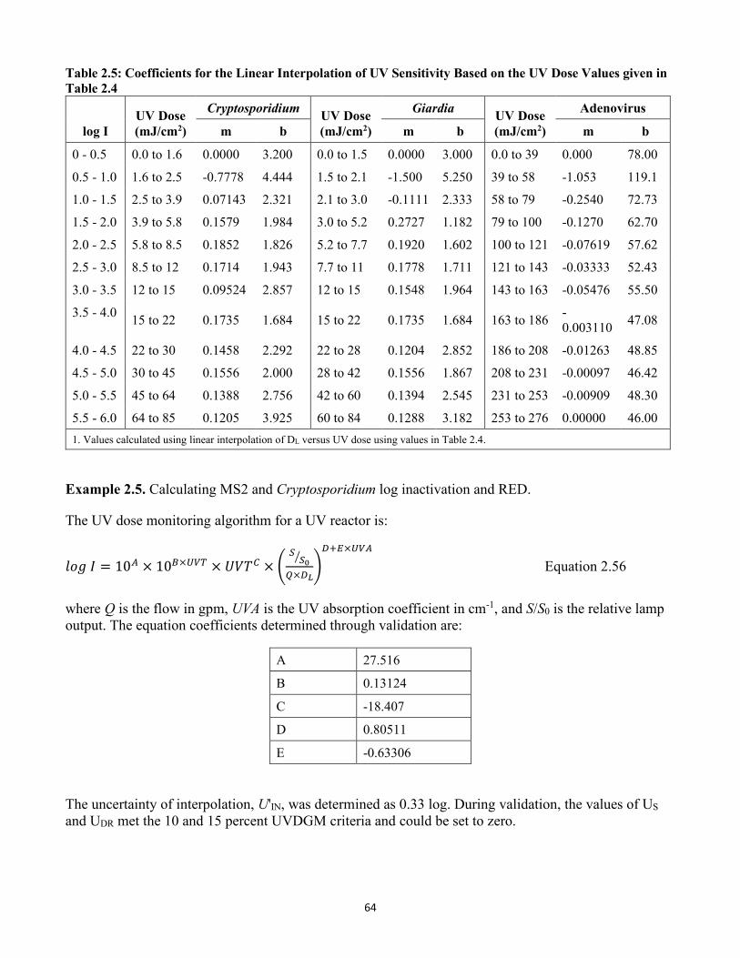
64

Table 2.5: Coefficients for the Linear Interpolation of UV Sensitivity Based on the UV Dose Values given in Table 2.4

log I UV Dose (mJ/cm2)

Cryptosporidium UV Dose (mJ/cm2)

Giardia UV Dose (mJ/cm2)

Adenovirus

m b m b m b

0 - 0.5 0.0 to 1.6 0.0000 3.200 0.0 to 1.5 0.0000 3.000 0.0 to 39 0.000 78.00

0.5 - 1.0 1.6 to 2.5 -0.7778 4.444 1.5 to 2.1 -1.500 5.250 39 to 58 -1.053 119.1

1.0 - 1.5 2.5 to 3.9 0.07143 2.321 2.1 to 3.0 -0.1111 2.333 58 to 79 -0.2540 72.73

1.5 - 2.0 3.9 to 5.8 0.1579 1.984 3.0 to 5.2 0.2727 1.182 79 to 100 -0.1270 62.70

2.0 - 2.5 5.8 to 8.5 0.1852 1.826 5.2 to 7.7 0.1920 1.602 100 to 121 -0.07619 57.62

2.5 - 3.0 8.5 to 12 0.1714 1.943 7.7 to 11 0.1778 1.711 121 to 143 -0.03333 52.43

3.0 - 3.5 12 to 15 0.09524 2.857 12 to 15 0.1548 1.964 143 to 163 -0.05476 55.50

3.5 - 4.0 15 to 22 0.1735 1.684 15 to 22 0.1735 1.684 163 to 186 -0.003110 47.08

4.0 - 4.5 22 to 30 0.1458 2.292 22 to 28 0.1204 2.852 186 to 208 -0.01263 48.85

4.5 - 5.0 30 to 45 0.1556 2.000 28 to 42 0.1556 1.867 208 to 231 -0.00097 46.42

5.0 - 5.5 45 to 64 0.1388 2.756 42 to 60 0.1394 2.545 231 to 253 -0.00909 48.30

5.5 - 6.0 64 to 85 0.1205 3.925 60 to 84 0.1288 3.182 253 to 276 0.00000 46.00 1. Values calculated using linear interpolation of DL versus UV dose using values in Table 2.4.

Example 2.5. Calculating MS2 and Cryptosporidium log inactivation and RED.

The UV dose monitoring algorithm for a UV reactor is:

𝑉𝑉𝐷𝐷𝑙𝑙 𝐼𝐼 = 10𝐴𝐴 × 10𝐵𝐵×𝑈𝑈𝑈𝑈𝑈𝑈 × 𝑈𝑈𝑉𝑉𝑈𝑈𝐶𝐶 × �𝑆𝑆𝑆𝑆0�

𝑄𝑄×𝑅𝑅𝐿𝐿�𝑅𝑅+𝑅𝑅×𝑈𝑈𝑈𝑈𝐴𝐴

Equation 2.56

where Q is the flow in gpm, UVA is the UV absorption coefficient in cm-1, and S/S0 is the relative lamp output. The equation coefficients determined through validation are:

A 27.516

B 0.13124

C -18.407

D 0.80511

E -0.63306

The uncertainty of interpolation, U'IN, was determined as 0.33 log. During validation, the values of US and UDR met the 10 and 15 percent UVDGM criteria and could be set to zero.

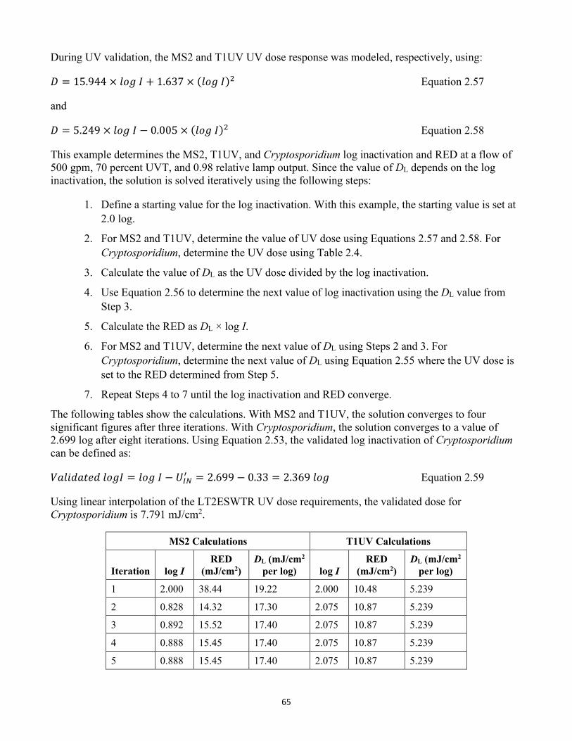
65

During UV validation, the MS2 and T1UV UV dose response was modeled, respectively, using:

𝐷𝐷 = 15.944 × 𝑉𝑉𝐷𝐷𝑙𝑙 𝐼𝐼 + 1.637 × (𝑉𝑉𝐷𝐷𝑙𝑙 𝐼𝐼)2 Equation 2.57

and

𝐷𝐷 = 5.249 × 𝑉𝑉𝐷𝐷𝑙𝑙 𝐼𝐼 − 0.005 × (𝑉𝑉𝐷𝐷𝑙𝑙 𝐼𝐼)2 Equation 2.58

This example determines the MS2, T1UV, and Cryptosporidium log inactivation and RED at a flow of 500 gpm, 70 percent UVT, and 0.98 relative lamp output. Since the value of DL depends on the log inactivation, the solution is solved iteratively using the following steps:

1. Define a starting value for the log inactivation. With this example, the starting value is set at 2.0 log.

2. For MS2 and T1UV, determine the value of UV dose using Equations 2.57 and 2.58. For Cryptosporidium, determine the UV dose using Table 2.4.

3. Calculate the value of DL as the UV dose divided by the log inactivation.

4. Use Equation 2.56 to determine the next value of log inactivation using the DL value from Step 3.

5. Calculate the RED as DL × log I.

6. For MS2 and T1UV, determine the next value of DL using Steps 2 and 3. For Cryptosporidium, determine the next value of DL using Equation 2.55 where the UV dose is set to the RED determined from Step 5.

7. Repeat Steps 4 to 7 until the log inactivation and RED converge.

The following tables show the calculations. With MS2 and T1UV, the solution converges to four significant figures after three iterations. With Cryptosporidium, the solution converges to a value of 2.699 log after eight iterations. Using Equation 2.53, the validated log inactivation of Cryptosporidium can be defined as:

𝑉𝑉𝑉𝑉𝑉𝑉𝑉𝑉𝑉𝑉𝑉𝑉𝑡𝑡𝑡𝑡𝑉𝑉 𝑉𝑉𝐷𝐷𝑙𝑙𝐼𝐼 = 𝑉𝑉𝐷𝐷𝑙𝑙 𝐼𝐼 − 𝑈𝑈𝐼𝐼𝐼𝐼′ = 2.699 − 0.33 = 2.369 𝑉𝑉𝐷𝐷𝑙𝑙 Equation 2.59

Using linear interpolation of the LT2ESWTR UV dose requirements, the validated dose for Cryptosporidium is 7.791 mJ/cm2.

MS2 Calculations T1UV Calculations

Iteration log I RED

(mJ/cm2) DL (mJ/cm2

per log) log I RED

(mJ/cm2) DL (mJ/cm2

per log)

1 2.000 38.44 19.22 2.000 10.48 5.239

2 0.828 14.32 17.30 2.075 10.87 5.239

3 0.892 15.52 17.40 2.075 10.87 5.239

4 0.888 15.45 17.40 2.075 10.87 5.239

5 0.888 15.45 17.40 2.075 10.87 5.239

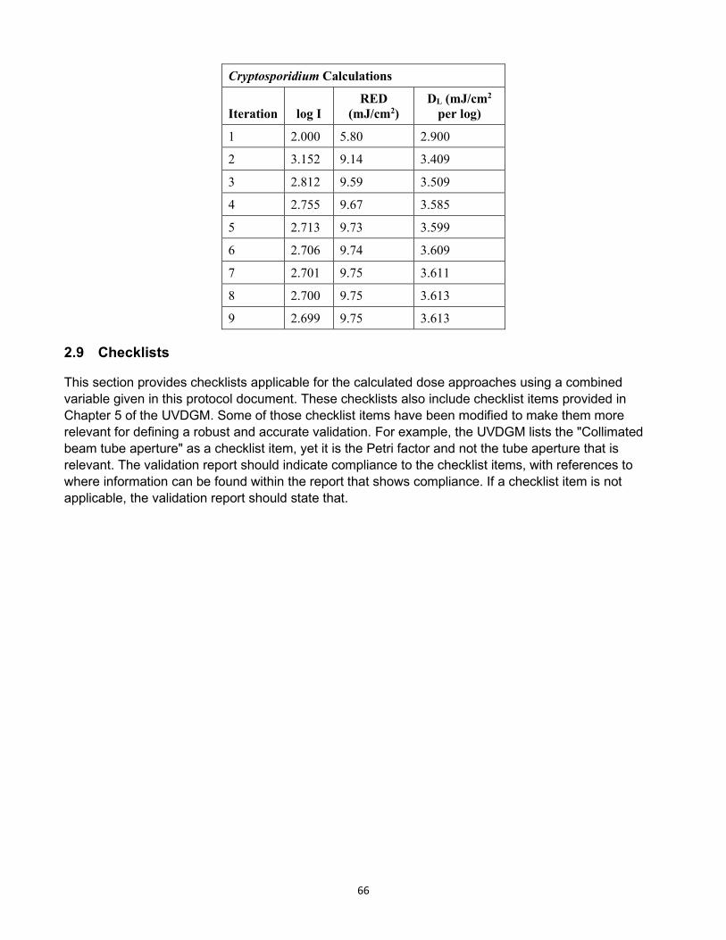
66

Cryptosporidium Calculations

Iteration log I RED

(mJ/cm2) DL (mJ/cm2

per log)

1 2.000 5.80 2.900

2 3.152 9.14 3.409

3 2.812 9.59 3.509

4 2.755 9.67 3.585

5 2.713 9.73 3.599

6 2.706 9.74 3.609

7 2.701 9.75 3.611

8 2.700 9.75 3.613

9 2.699 9.75 3.613

2.9 Checklists

This section provides checklists applicable for the calculated dose approaches using a combined variable given in this protocol document. These checklists also include checklist items provided in Chapter 5 of the UVDGM. Some of those checklist items have been modified to make them more relevant for defining a robust and accurate validation. For example, the UVDGM lists the "Collimated beam tube aperture" as a checklist item, yet it is the Petri factor and not the tube aperture that is relevant. The validation report should indicate compliance to the checklist items, with references to where information can be found within the report that shows compliance. If a checklist item is not applicable, the validation report should state that.

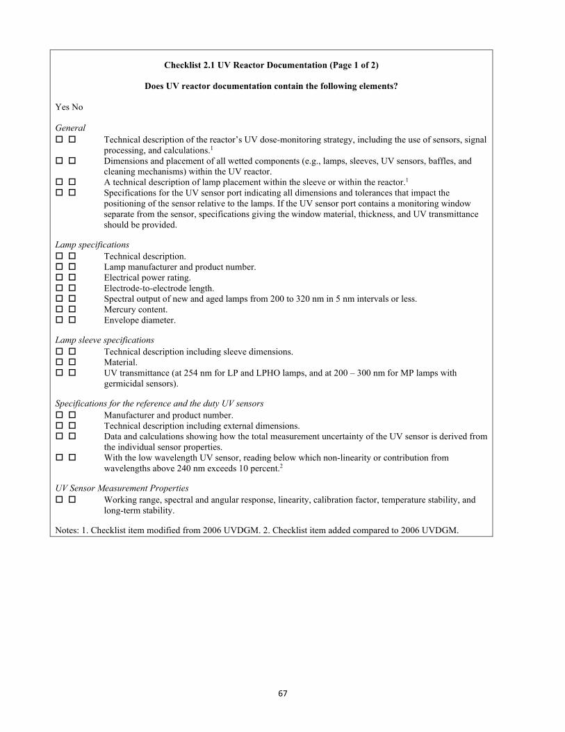
67

Checklist 2.1 UV Reactor Documentation (Page 1 of 2)

Does UV reactor documentation contain the following elements?

Yes No

General Technical description of the reactor’s UV dose-monitoring strategy, including the use of sensors, signal

processing, and calculations.1

Dimensions and placement of all wetted components (e.g., lamps, sleeves, UV sensors, baffles, and cleaning mechanisms) within the UV reactor.

A technical description of lamp placement within the sleeve or within the reactor.1

Specifications for the UV sensor port indicating all dimensions and tolerances that impact the positioning of the sensor relative to the lamps. If the UV sensor port contains a monitoring window separate from the sensor, specifications giving the window material, thickness, and UV transmittance should be provided.

Lamp specifications Technical description. Lamp manufacturer and product number. Electrical power rating. Electrode-to-electrode length. Spectral output of new and aged lamps from 200 to 320 nm in 5 nm intervals or less. Mercury content. Envelope diameter.

Lamp sleeve specifications Technical description including sleeve dimensions. Material. UV transmittance (at 254 nm for LP and LPHO lamps, and at 200 – 300 nm for MP lamps with

germicidal sensors).

Specifications for the reference and the duty UV sensors Manufacturer and product number. Technical description including external dimensions. Data and calculations showing how the total measurement uncertainty of the UV sensor is derived from

the individual sensor properties. With the low wavelength UV sensor, reading below which non-linearity or contribution from

wavelengths above 240 nm exceeds 10 percent.2

UV Sensor Measurement Properties Working range, spectral and angular response, linearity, calibration factor, temperature stability, and

long-term stability.

Notes: 1. Checklist item modified from 2006 UVDGM. 2. Checklist item added compared to 2006 UVDGM.

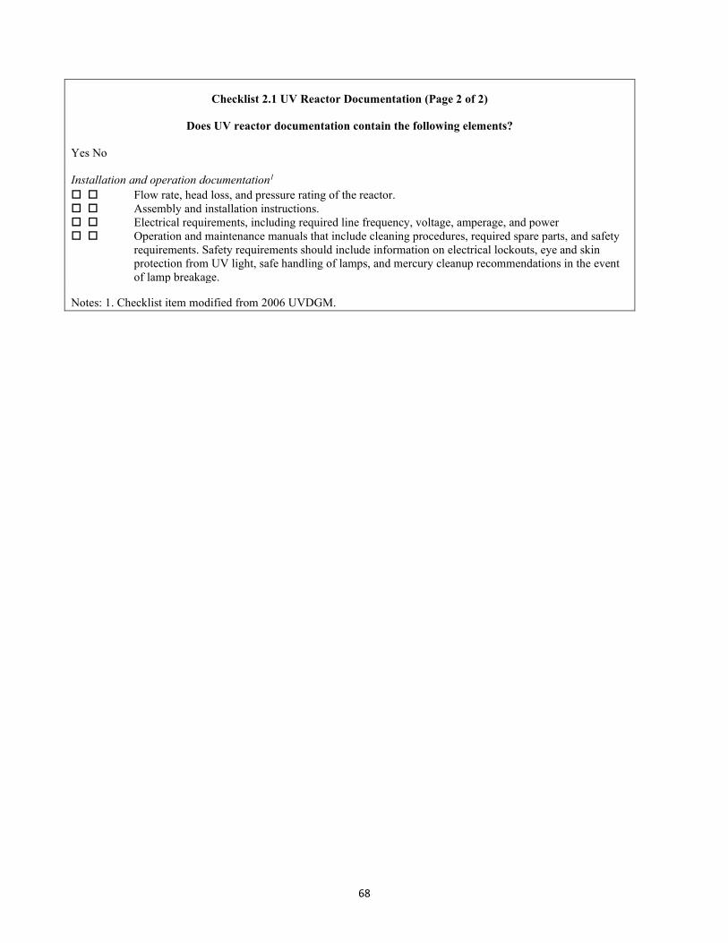
68

Checklist 2.1 UV Reactor Documentation (Page 2 of 2)

Does UV reactor documentation contain the following elements?

Yes No

Installation and operation documentation1

Flow rate, head loss, and pressure rating of the reactor. Assembly and installation instructions. Electrical requirements, including required line frequency, voltage, amperage, and power Operation and maintenance manuals that include cleaning procedures, required spare parts, and safety

requirements. Safety requirements should include information on electrical lockouts, eye and skin protection from UV light, safe handling of lamps, and mercury cleanup recommendations in the event of lamp breakage.

Notes: 1. Checklist item modified from 2006 UVDGM.

69

Checklist 2.2 Key Elements of the Validation Test Plan (Page 1 of 1)

Does the validation test plan contain the following elements?

Yes No

General Purpose of Validation Testing. General description of why the tests are being done and how the data

will be used. Roles and Responsibilities. Key personnel overseeing and performing the full-scale reactor testing and

collimated beam testing, including their qualifications. This section should include contact names and telephone numbers.

Locations and Schedule. Location for conducting full-scale reactor testing and collimated beam testing. Planned schedule for conducting the tests and performing the data analyses.

Challenge Microorganism. Protocols for growth and enumeration, expected UV dose-response, and suitability for use in validation testing.1

Plan for state review (if applicable).

Design of the Biodosimetry Test Stand/On-site Testing Facilities1

Inlet/outlet piping design from a location 5 pipe diameters upstream of the inlet injection point to a location downstream of the effluent sampling port.1

Mixing of injected UV absorbers and challenge microorganisms.1 Sample ports. UV absorber and challenge microorganisms feed pumps.1 Additives (Material Safety Data Sheets for UV-absorbing chemical, quenching agent).

Collimated Beam Testing Apparatus 1

Lamp type. Petri factor.1

Distance from light source to sample surface. Radiometer make, model, and calibration certificate.

Monitoring Equipment Specifications and Verification of Equipment Accuracy for the following:1

Flow meters. UVT analyzers (if used). UV Spectrophotometers. Power meters.1 Duty and reference UV sensors.1 Radiometer make, model, and calibration certificates

Experimental Test Conditions including, but not limited to: Number of tests, UVT, flow rate, lamp power, and lamp status for each test condition. Use of new and/or aged lamps.1

Influent concentration of challenge microorganisms for each test condition. QA/QC Plan. Notes: 1. Checklist item modified from 2006 UVDGM.

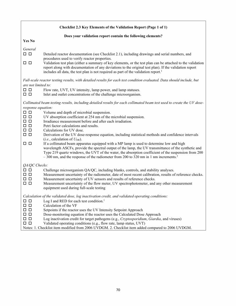
70

Checklist 2.3 Key Elements of the Validation Report (Page 1 of 1)

Does your validation report contain the following elements? Yes No

General Detailed reactor documentation (see Checklist 2.1), including drawings and serial numbers, and

procedures used to verify reactor properties. Validation test plan (either a summary of key elements, or the test plan can be attached to the validation

report along with documentation of any deviations to the original test plan). If the validation report includes all data, the test plan is not required as part of the validation report.1

Full-scale reactor testing results, with detailed results for each test condition evaluated. Data should include, but are not limited to: Flow rate, UVT, UV intensity, lamp power, and lamp statuses. Inlet and outlet concentrations of the challenge microorganism.

Collimated beam testing results, including detailed results for each collimated beam test used to create the UV dose-response equation: Volume and depth of microbial suspension. UV absorption coefficient at 254 nm of the microbial suspension. Irradiance measurement before and after each irradiation. Petri factor calculations and results. Calculations for UV dose. Derivation of the UV dose-response equation, including statistical methods and confidence intervals

(i.e., calculation of UDR). If a collimated beam apparatus equipped with a MP lamp is used to determine low and high

wavelength ASCFs, provide the spectral output of the lamp, the UV transmittance of the synthetic and Type 219 quartz windows, the UVT of the water, the absorption coefficient of the suspension from 200 – 300 nm, and the response of the radiometer from 200 to 320 nm in 1 nm increments.2

QA/QC Checks: Challenge microorganism QA/QC, including blanks, controls, and stability analyses. Measurement uncertainty of the radiometer, date of most recent calibration, results of reference checks. Measurement uncertainty of UV sensors and results of reference checks. Measurement uncertainty of the flow meter, UV spectrophotometer, and any other measurement

equipment used during full-scale testing

Calculation of the validated dose, log inactivation credit, and validated operating conditions: Log I and RED for each test condition.1

Calculation of the VF Setpoints if the reactor uses the UV Intensity Setpoint Approach Dose-monitoring equation if the reactor uses the Calculated Dose Approach Log inactivation credit for target pathogens (e.g., Cryptosporidium, Giardia, and viruses) Validated operating conditions (e.g., flow rate, lamp status, UVT) Notes: 1. Checklist item modified from 2006 UVDGM. 2. Checklist item added compared to 2006 UVDGM.

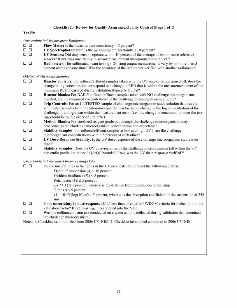
71

Checklist 2.4 Review for Quality Assurance/Quality Control (Page 1 of 1) Yes No

Uncertainty in Measurement Equipment Flow Meter: Is the measurement uncertainty < 5 percent? UV Spectrophotometer: Is the measurement uncertainty < 10 percent? UV Sensors: Did duty sensors operate within 10 percent of the average of two or more reference

sensors? If not, was uncertainty in sensor measurement incorporated into the VF? Radiometer: (for collimated beam testing). Do lamp output measurements vary by no more than 5

percent over exposure time? Was the accuracy of the radiometer verified with another radiometer?

QA/QC of Microbial Samples Reactor controls: For influent/effluent samples taken with the UV reactor lamps turned off, does the

change in log concentration correspond to a change in RED that is within the measurement error of the minimum RED measured during validation (typically ≤ 3 %)?

Reactor blanks: For DAILY influent/effluent samples taken with NO challenge microorganisms injected, are the measured concentrations of the challenge microorganism negligible?

Trip Controls: For an UNTESTED sample of challenge microorganism stock solution that travels with tested samples from the laboratory and the reactor, is the change in the log concentration of the challenge microorganism within the measurement error. (i.e., the change in concentration over the test run should be on the order of 3 to 5 %.)

Method Blanks: For sterilized reagent grade put through the challenge microorganism assay procedure, is the challenge microorganism concentration non-detectable?

Stability Samples: For influent/effluent samples at low and high UVT, are the challenge microorganism concentrations within 5 percent of each other?

UV Dose-Response Stability: Is the UV dose-response of the challenge microorganism stable over time?2

Stability Samples: Does the UV dose-response of the challenge microorganism fall within the 95th percentile prediction interval QA/QC bounds? If not, was the UV dose-response verified?2

Uncertainty in Collimated Beam Testing Data Do the uncertainties in the terms in the UV dose calculation meet the following criteria:

Depth of suspension (d) ≤ 10 percent Incident irradiance (Es) ≤ 8 percent Petri factor (Pf) ≤ 5 percent L/(d + L) ≤ 1 percent, where L is the distance from the solution to the lamp Time (t) ≤ 5 percent (1 – 10-ad)/(log(10)ad) ≤ 5 percent, where a is the absorption coefficient of the suspension at 254 nm

Is the uncertainty in dose-response (UDR) less than or equal to UVDGM criteria for inclusion into the validation factor? If not, was UDR incorporated into the VF?

Was the collimated beam test conducted on a water sample collected during validation that contained the challenge microorganism?1


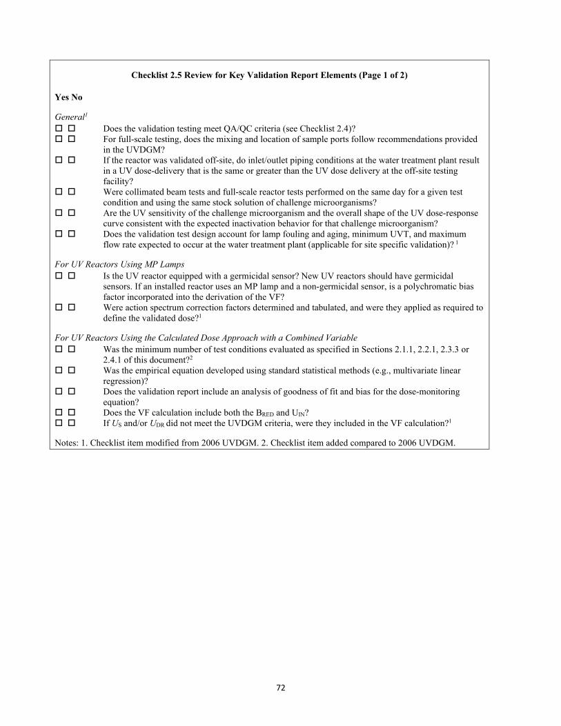
72

Checklist 2.5 Review for Key Validation Report Elements (Page 1 of 2) Yes No

General1

Does the validation testing meet QA/QC criteria (see Checklist 2.4)? For full-scale testing, does the mixing and location of sample ports follow recommendations provided

in the UVDGM? If the reactor was validated off-site, do inlet/outlet piping conditions at the water treatment plant result

in a UV dose-delivery that is the same or greater than the UV dose delivery at the off-site testing facility?

Were collimated beam tests and full-scale reactor tests performed on the same day for a given test condition and using the same stock solution of challenge microorganisms?

Are the UV sensitivity of the challenge microorganism and the overall shape of the UV dose-response curve consistent with the expected inactivation behavior for that challenge microorganism?

Does the validation test design account for lamp fouling and aging, minimum UVT, and maximum flow rate expected to occur at the water treatment plant (applicable for site specific validation)? 1

For UV Reactors Using MP Lamps Is the UV reactor equipped with a germicidal sensor? New UV reactors should have germicidal

sensors. If an installed reactor uses an MP lamp and a non-germicidal sensor, is a polychromatic bias factor incorporated into the derivation of the VF?

Were action spectrum correction factors determined and tabulated, and were they applied as required to define the validated dose?1

For UV Reactors Using the Calculated Dose Approach with a Combined Variable Was the minimum number of test conditions evaluated as specified in Sections 2.1.1, 2.2.1, 2.3.3 or

2.4.1 of this document?2

Was the empirical equation developed using standard statistical methods (e.g., multivariate linear regression)?

Does the validation report include an analysis of goodness of fit and bias for the dose-monitoring equation?

Does the VF calculation include both the BRED and UIN? If US and/or UDR did not meet the UVDGM criteria, were they included in the VF calculation?1


73

2.10 Use of Alternate Lamps

The UV system manufacturer may modify the lamp or ballast used by the UV system to improve lamp output and improve reliability. While the UV dose monitoring algorithm developed in accordance with Section 2.1, 2.2, 2.3, or 2.4 may be used with the UV reactor equipped with modified lamps and/or ballasts, the validity of the algorithm should be evaluated on a case-by-case basis by the validator who will provide an addendum for the validation report describing the results of the evaluation. While the UV dose monitoring algorithm may be used with a modified lamp and/or ballast that provides greater UV output, the algorithm can only be used within the validated range; greater UV output does not extend the validated range of log inactivation.

The new lamp should have the same arc length and envelope diameter as the original lamp, and should have the same relative lamp output (uniformity) along the length and about the circumference of the lamp. MP lamps may have a non-uniform output about their circumference and amalgam LPHO lamps may have a non-uniform output along their length (Wright et al., 2007). With MP lamps, the new lamp should also have the same relative spectral output. The spectral output can be evaluated by comparing the germicidal output defined as:

( ) ( ) λλλλ

∆= ∑ 2MSG GPP Equation 2.60

where PG is the germicidal output, P(λ) is the measured UV output of the lamp defined as a function of wavelength, GMS2(λ) is the action spectra of MS2 phage defined as a function of wavelength, and Δλ is a wavelength increment no greater than 5 nm.

UV intensity models and CFD-based UV dose models can be used to quantify the impact of the two lamp types on UV dose delivery and UV sensor readings. If CFD-based UV dose models are used, they should be validated per the recommendations of Linden et al. (2015). The comparison of UV dose delivery with the new lamp is done for the same relative lamp output (i.e., S/S0). If the log inactivation predicted with the new lamp is greater than the log inactivation predicted with the validation, the equation predicting log inactivation developed through validation may be used for UV dose monitoring with the new lamp. If log inactivation predicted with the new lamp is lower than with the validation but within the uncertainty of interpolation as defined by Equation 2.51, the log inactivation equations developed through validation may be used provided that the log inactivation predicted by the equation is multiplied by a factor defined as the smallest value of the ratio of the log inactivation with the new lamp divided by the log inactivation with the validation lamp observed with the CFD-based UV dose model predictions. If the log inactivation with the new lamp is lower than the validation by more than the uncertainty of interpolation, the validation equations cannot be used for the installation.

The addendum should also provide a comparison of the measured UV sensor readings as a function of ballast power for the original and new lamp and/or ballast. The data should be used to define the lamp output used for sizing the UV system equipped with the new lamp and/or ballast.

If the UV dose monitoring algorithm was developed in accordance with Sections 2.2 or 2.4 and the new lamp has a greater UV output at 100 percent power compared to the original lamp, the optimal UV sensor position should be re-analyzed per Section 2.2.5 or 2.4.4, respectively.

74

3.0 General UV Validation and Monitoring Procedures This chapter provides recommendations on UV validation and monitoring procedures.


3.1. Determining UV Dose Response Using a Collimated Beam.

3.2. Test Conditions for the UV Intensity Setpoint Approach.

3.3. Linear Scaling of Log Inactivation by UV Sensor Readings.

3.4. Selecting and Applying the RED Bias.

3.5. Calculating the Uncertainty of the UV Dose Response, UDR.

3.6. Applying Action Spectrum Correction Factors Based on Linden et al. (2015).

3.7. Duty UV Sensor Calibration.

3.8. Online UVT Monitor QA/QC Criteria.

3.9. Lamp-To-Lamp Variability.

3.10. t-Statistics.

3.11 UV Reactors with Enhanced Reflection.

3.12 Role of CFD-based UV Dose Models.

3.1 Determining UV Dose Response using a Collimated Beam

Appendix C of the UVDGM describes the determination of the challenge microorganism's UV dose-response using a collimated beam apparatus. The following approaches are recommended to improve the accuracy of the measured UV dose-response:

1. The UVDGM recommends that the value of log N0, the log concentration of the challenge microorganism measured with zero UV dose, is obtained using the fit to the dose-response expressed as log N versus UV dose. With UV dose-response that shows curvature, the estimates of log N0 using this approach can be biased low or high. If these biases occur, log N0 should be calculated as the average value of the data measured with a zero UV dose.

2. The UVDGM recommends that the UV dose-response be modeled using a linear or quadratic equation. Other equations are acceptable if they account for any shoulders or curvature in the UV dose-response such that the differences between the measured and predicted dose-response are not biased.

75

3. The accuracy of the UV dose-response measured using the collimated beam apparatus is dependent on the accuracy of the radiometer used to measure the UV intensity used in the UV dose calculation. Because radiometer calibration can have a significant error that biases the UV dose calculations, the UV intensity should be measured using at least three radiometers, including at least one from a different manufacturer, and those radiometers should have NIST-traceable calibration or equivalent completed within the past year prior to use. If multiple radiometers from one manufacturer are used, the calibrations of those radiometers should be staggered over time as opposed to being done at the same time to prevent the same calibration error biasing all radiometers. Actinometry can also be used to check the calibration of the radiometers. Control charts should be used to evaluate how the radiometer calibration changes over time and inspected after each calibration to identify any significant change in the calibration process. The average UV intensity made by multiple radiometers should be used to calculate the UV dose delivered by the collimated beam apparatus.

4. With the collimated beam irradiations, if the height of the glass dish holding the water sample is greater than the sample depth, UV light will be reflected off the inside walls of the dish and into the sample, thereby increasing the UV dose delivered to the sample (Verhoeven et al., 2011). The UV dose calculation for the collimated beam device provided in the UVDGM does not account for this effect. To address this issue, the contribution of reflected UV light from the side walls of the dish into the water sample should be minimized by using a vessel height that does not significantly exceed the suspension depth. Note that if this issue were to occur, the outcome would be conservative since the RED assigned to the UV reactor would be lower than would have been assigned otherwise.

5. The UVDGM states that the concentration of the challenge microorganisms in the validation samples should be stable over time but does not address the stability of the UV dose-response. The UV dose-response of the challenge microorganisms should be stable over time and unaffected by the water matrix.

6. The UV dose-response should be measured on a sample containing the challenge microorganisms collected during validation testing. This water sample can be spiked with the challenge microorganism at the time of collection to extend the range of log inactivation with the UV dose-response to higher values that may have been measured through the UV reactor during validation testing. However, tests should be done to verify that the UV dose-response of the spiked and unspiked samples are the same.

3.2 Test Conditions for the UV Intensity Setpoint Approach

With the UV intensity setpoint approach, the UV reactor delivers a required UV dose or greater when the UV sensor reads above a target value. The validation testing of the UV intensity setpoint approach involves two test conditions for each flow rate evaluated:

1. High UVT and lamp power lowered until the UV sensor reads at the setpoint value

2. 100 percent power and UVT lowered until the UV sensor reads at the setpoint value

The reactor is rated at the lower of the two REDs measured with the two test conditions. Which test condition gives the lowest RED depends on the distance between the UV sensor and the lamps. If the

76

UV sensor is located relatively far from the lamps, test 1 gives the lowest RED. If the UV sensor is located close to the lamps, test 2 gives the lowest RED. To provide the most cost-efficient application of UV light, UV system manufacturers using the UV intensity setpoint approach place their UV sensor at an intermediate position to minimize RED differences between the two test conditions. This UV sensor location is referred to in the UVDGM as the “optimal” UV sensor position for setpoint monitoring. An underlying assumption of this approach is that the RED delivered at intermediate UVTs with the reactor operating at the setpoint will lie between the two measured UVTs.

As shown in Appendix A (Section A.5), with the UV sensor at the optimal location, the log inactivation and associated RED delivered at intermediate UVTs can be lower than the REDs measured with the two validation test conditions. As such, it is recommended that the UV intensity setpoint approach include test points measured at intermediate UVTs with the ballast power lowered until the UV sensor reads at the setpoint value. Those intermediate UVTs can be defined using the approach described in Section 2.1.1 that uses Equation 2.6.

The German Deutscher Verein des Gas- und Wasserfaches (DVGW) and the Austrian Osterreichisches Normungsinstitut (ÖNORM) protocols validate UV systems for a B. subtilis RED of 40 mJ/cm2 using the UV intensity setpoint approach. Many of those validations have used two test conditions as described above. Section 5.2.2 of the UVDGM states that UV reactors certified by DVGW and ÖNORM for a B. subtilis RED of 40 mJ/cm2 should be granted 3-log Cryptosporidium and 3-log Giardia inactivation credit. Wright (2007) provides analysis that shows the validated dose for Cryptosporidium and Giardia inactivation credit expected with a B. subtilis RED of 40 mJ/cm2 after applying a validation factor calculated per the UVDGM. The analysis shows that a B. subtilis RED of 40 mJ/cm2 conservatively achieves 3-log inactivation credit with Cryptosporidium and Giardia for UVTs ranging from 70 to 98 percent. Based on this analysis, a UV system designed and operated to deliver a B. subtilis or MS2 RED of 40 mJ/cm2 based on the UV intensity setpoint approach per the UVDGM can still be considered to achieve 3-log inactivation credit with Cryptosporidium and Giardia. However, UV systems designed and operated to deliver B. subtilis or MS2 REDs that are lower than 40 mJ/cm2, based on the UV intensity setpoint per the UVDGM, should be evaluated on a case-by-case basis by the validation facility for disinfection credit, addressing the issues raised in this section.

3.3 Linear Scaling of Log Inactivation by UV Sensor Readings

As shown in Figure A.7, the relation between log inactivation and the combined variable is always concave downward (i.e., the slope decreases with higher values of the combined variable). For a given flow, UVT and microbe, this is also true for the relation between log inactivation and the UV sensor readings or the relative lamp output. For this reason, the log inactivation or RED can be linearly interpolated as a function of UV sensor readings or the relative lamp output down to a zero. This interpolation down to zero will be conservative because the relation between log inactivation and UV sensor readings is always concave downward.

Linear extrapolation to higher UV sensor readings or relative lamp outputs should not be done because the extrapolation will not be conservative.

Linear interpolation of log inactivation or RED as a function of UV sensor readings is useful if validation was limited by ballast power settings (e.g., the lamps could only operate at 100 percent power).

77

3.4 Selecting and Applying the RED bias

Appendix G of the UVDGM tabulates recommended values for the RED bias factor as a function of log inactivation credit of the target pathogen, the UV sensitivity of the challenge microorganism, and the UVT of the water. The UV sensitivity of the challenge microorganism is obtained from the UV dose-response curve measured using the collimated beam apparatus and calculated using:

𝐷𝐷𝐿𝐿 = 𝐷𝐷𝑉𝑉𝐷𝐷𝑙𝑙 𝐼𝐼� Equation 3.1

where D is the UV dose and log I is the log inactivation of the challenge microorganism expected with a given UV dose.

Section 5.9.1 of the UVDGM recommends determining the RED bias using the maximum value of DL observed with the test condition replicate conducted at the lowest UVT. However, the UV dose-responses of the challenge microorganisms do not depend on UVT, the UV dose-response curve is not necessarily measured at the lowest UVT for a given day of testing, and the RED measured at the lowest UVT could be a low number or a high number depending on other variables such as flow and ballast power. As an alternative to this approach, this document recommends determining the RED bias using the value of DL observed with the challenge microorganism's UV dose-response measured during validation. If the UV dose-response curve of the challenge microorganism shows curvature, as is the case with MS2 phage, the value of DL will vary with the UV dose or RED, increasing in value at higher UV doses or REDs. If the UV dose-monitoring algorithm uses DL as an input to the algorithm, the value of DL used within the algorithm should be used to determine the RED bias.

The UVDGM currently provides values for the RED bias factor for 0.5 to 4.0 log inactivation credit of Cryptosporidium and Giardia at UVTs that range from 65 to 98 percent. As shown in Figure 3.1, for UVTs from 65 to 85 percent, the RED bias factors in the UVDGM are described well using a linear function. As such, for UVTs less than 65 percent, the RED bias factors may be estimated using a linear extrapolation of the UVDGM values tabulated at 65 and 75 percent UVT. Furthermore, Figure 3.1 shows that the RED bias factors in the UVDGM at a given UVT and UV dose per log inactivation decrease with increased log inactivation credit. Hence, the RED bias factors for 4.0 log inactivation credit can be conservatively used for log inactivation greater than 4.0 log.

If the UV dose monitoring algorithm developed using the validation data accounts for the UV dose per log reduction of the microbe (i.e., DL), the estimated RED bias factor from the UVDGM can be compared to the actual RED bias of the UV reactor calculated using the algorithm. The comparison can be used to justify use of the estimated value.

Example 3.1. Comparison of a UV reactor's actual RED Bias to UVDGM RED bias factors.

With Example 2.5, the UV dose monitoring algorithm given by Equation 2.56 was used to predict MS2 and Cryptosporidium REDs of 15.45 and 9.75 mJ/cm2, respectively, at a UVT of 70 percent. The MS2 DL was 17.40 mJ/cm2 per log. The UV reactor's actual RED bias for MS2 relative to Cryptosporidium is 15.45/9.75 = 1.584. The RED bias factor at 70 percent UVT, taken from Table G.4 of the UVDGM, is ~2.72. As shown, the RED bias factors given in the UVDGM are conservative for this particular UV reactor.

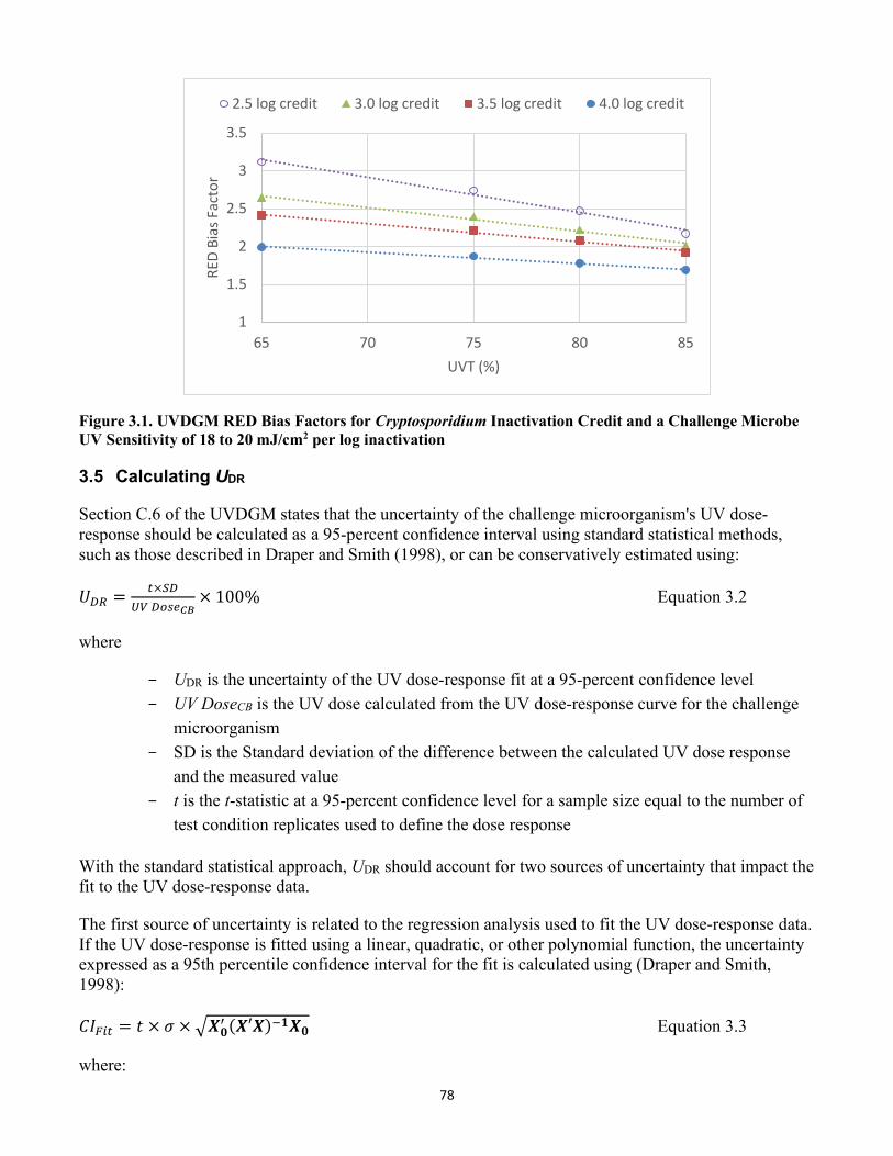
78

1

1.5

2

2.5

3

3.5

65 70 75 80 85

RED

Bias

Fac

tor

UVT (%)

2.5 log credit 3.0 log credit 3.5 log credit 4.0 log credit

Figure 3.1. UVDGM RED Bias Factors for Cryptosporidium Inactivation Credit and a Challenge Microbe UV Sensitivity of 18 to 20 mJ/cm2 per log inactivation

3.5 Calculating UDR

Section C.6 of the UVDGM states that the uncertainty of the challenge microorganism's UV dose-response should be calculated as a 95-percent confidence interval using standard statistical methods, such as those described in Draper and Smith (1998), or can be conservatively estimated using:

𝑈𝑈𝑅𝑅𝑅𝑅 = 𝑡𝑡×𝑆𝑆𝑅𝑅𝑈𝑈𝑈𝑈 𝑅𝑅𝑃𝑃𝐷𝐷𝑒𝑒𝐶𝐶𝐶𝐶


where

UDR is the uncertainty of the UV dose-response fit at a 95-percent confidence level UV DoseCB is the UV dose calculated from the UV dose-response curve for the challenge

microorganism SD is the Standard deviation of the difference between the calculated UV dose response

and the measured value t is the t-statistic at a 95-percent confidence level for a sample size equal to the number of

test condition replicates used to define the dose response

With the standard statistical approach, UDR should account for two sources of uncertainty that impact the fit to the UV dose-response data.

The first source of uncertainty is related to the regression analysis used to fit the UV dose-response data. If the UV dose-response is fitted using a linear, quadratic, or other polynomial function, the uncertainty expressed as a 95th percentile confidence interval for the fit is calculated using (Draper and Smith, 1998):

𝐴𝐴𝐼𝐼𝐹𝐹𝑀𝑀𝑡𝑡 = 𝑡𝑡 × 𝜎𝜎 × �𝑿𝑿𝟎𝟎′ (𝑿𝑿′𝑿𝑿)−𝟏𝟏𝑿𝑿𝟎𝟎 Equation 3.3

where:

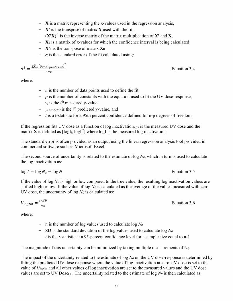
79

X is a matrix representing the x-values used in the regression analysis, X' is the transpose of matrix X used with the fit, (X'X)-1 is the inverse matrix of the matrix multiplication of X' and X, X0 is a matrix of x-values for which the confidence interval is being calculated X'0 is the transpose of matrix X0 σ is the standard error of the fit calculated using:

𝜎𝜎2 =∑ �𝑃𝑃𝑉𝑉−𝑃𝑃𝑉𝑉,𝑝𝑝𝑝𝑝𝑜𝑜𝑉𝑉𝑉𝑉𝑝𝑝𝑉𝑉𝑜𝑜𝑉𝑉�

2𝑉𝑉𝑉𝑉=1

𝑛𝑛−𝑝𝑝 Equation 3.4

where:

n is the number of data points used to define the fit p is the number of constants with the equation used to fit the UV dose-response, yi is the ith measured y-value yi,predicted is the ith predicted y-value, and t is a t-statistic for a 95th percent confidence defined for n-p degrees of freedom.

If the regression fits UV dose as a function of log inactivation, yi is the measured UV dose and the matrix X is defined as [logIi, logIi

2] where logI is the measured log inactivation.

The standard error is often provided as an output using the linear regression analysis tool provided in commercial software such as Microsoft Excel.

The second source of uncertainty is related to the estimate of log N0, which in turn is used to calculate the log inactivation as:

log 𝐼𝐼 = log𝑁𝑁0 − log𝑁𝑁 Equation 3.5

If the value of log N0 is high or low compared to the true value, the resulting log inactivation values are shifted high or low. If the value of log N0 is calculated as the average of the values measured with zero UV dose, the uncertainty of log N0 is calculated as:

𝑈𝑈𝑃𝑃𝑃𝑃𝐴𝐴𝐼𝐼0 = 𝑡𝑡×𝑆𝑆𝑅𝑅√𝑛𝑛

Equation 3.6

where:

n is the number of log values used to calculate log N0 SD is the standard deviation of the log values used to calculate log N0 t is the t-statistic at a 95-percent confidence level for a sample size equal to n-1

The magnitude of this uncertainty can be minimized by taking multiple measurements of N0.

The impact of the uncertainty related to the estimate of log N0 on the UV dose-response is determined by fitting the predicted UV dose response where the value of log inactivation at zero UV dose is set to the value of UlogNo and all other values of log inactivation are set to the measured values and the UV dose values are set to UV DoseCB. The uncertainty related to the estimate of log N0 is then calculated as:

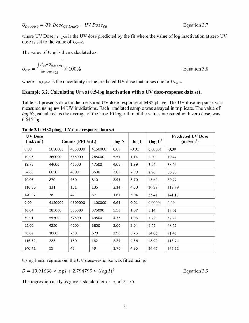
80

𝑈𝑈𝑅𝑅,𝑃𝑃𝑃𝑃𝐴𝐴𝐼𝐼0 = 𝑈𝑈𝑉𝑉 𝐷𝐷𝐷𝐷𝐷𝐷𝑡𝑡𝐶𝐶𝐵𝐵,𝑃𝑃𝑃𝑃𝐴𝐴𝐼𝐼0 − 𝑈𝑈𝑉𝑉 𝐷𝐷𝐷𝐷𝐷𝐷𝑡𝑡𝐶𝐶𝐵𝐵 Equation 3.7

where UV DoseCB,logN0 is the UV dose predicted by the fit where the value of log inactivation at zero UV dose is set to the value of UlogNo.

The value of UDR is then calculated as:

𝑈𝑈𝑅𝑅𝑅𝑅 =�𝑈𝑈𝐹𝐹𝑉𝑉𝑉𝑉

2 +𝑈𝑈𝐷𝐷,𝑉𝑉𝑉𝑉𝑜𝑜𝑙𝑙02

𝑈𝑈𝑈𝑈 𝑅𝑅𝑃𝑃𝐷𝐷𝑒𝑒𝐶𝐶𝐶𝐶× 100% Equation 3.8

where UD,logN0 is the uncertainty in the predicted UV dose that arises due to UlogNo.

Example 3.2. Calculating UDR at 0.5-log inactivation with a UV dose-response data set.

Table 3.1 presents data on the measured UV dose-response of MS2 phage. The UV dose-response was measured using n= 14 UV irradiations. Each irradiated sample was assayed in triplicate. The value of log N0, calculated as the average of the base 10 logarithm of the values measured with zero dose, was 6.645 log.

Table 3.1: MS2 phage UV dose-response data set UV Dose (mJ/cm2) Counts (PFU/mL) log N log I (log I)2

Predicted UV Dose (mJ/cm2)

0.00 5050000 4350000 4150000 6.65 -0.01 0.00004 -0.09

19.96 360000 365000 245000 5.51 1.14 1.30 19.47

39.75 44000 46500 47500 4.66 1.99 3.94 38.65

64.88 6050 4000 3500 3.65 2.99 8.96 66.70

90.03 870 980 810 2.95 3.70 13.69 89.77

116.55 131 151 136 2.14 4.50 20.29 119.39

140.07 38 47 37 1.61 5.04 25.41 141.17

0.00 4150000 4900000 4100000 6.64 0.01 0.00004 0.09

20.04 385000 385000 375000 5.58 1.07 1.14 18.02

39.91 55500 52500 49500 4.72 1.93 3.72 37.22

65.06 4250 4000 3800 3.60 3.04 9.27 68.27

90.02 1000 710 670 2.90 3.75 14.05 91.45

116.52 223 180 182 2.29 4.36 18.99 113.74

140.41 55 47 49 1.70 4.95 24.47 137.22 Using linear regression, the UV dose-response was fitted using:

𝐷𝐷 = 13.91666 × log 𝐼𝐼 + 2.794799 × (𝑉𝑉𝐷𝐷𝑙𝑙 𝐼𝐼)2 Equation 3.9

The regression analysis gave a standard error, σ, of 2.155.

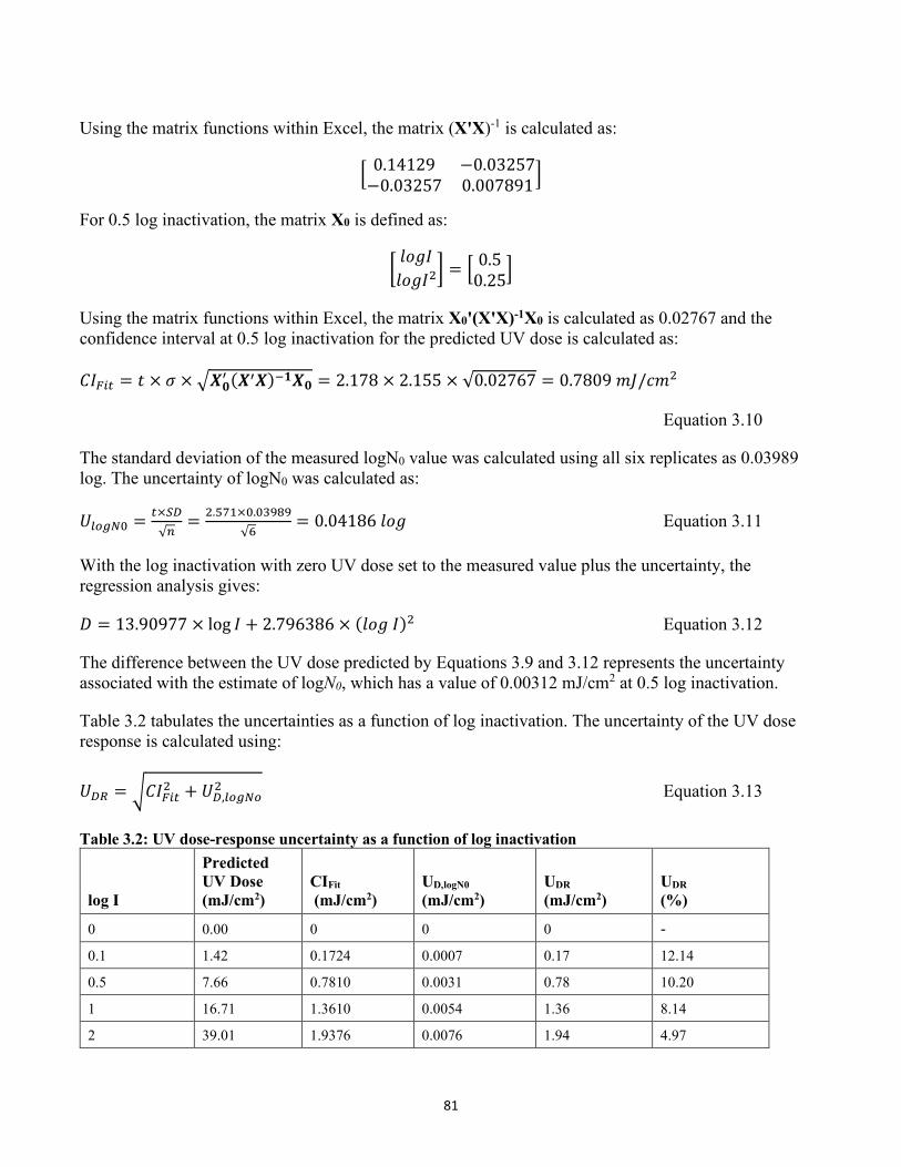
81

Using the matrix functions within Excel, the matrix (X'X)-1 is calculated as:

� 0.14129 −0.03257−0.03257 0.007891�

For 0.5 log inactivation, the matrix X0 is defined as:

�𝑉𝑉𝐷𝐷𝑙𝑙𝐼𝐼𝑉𝑉𝐷𝐷𝑙𝑙𝐼𝐼2� = � 0.5

0.25�

Using the matrix functions within Excel, the matrix X0'(X'X)-1X0 is calculated as 0.02767 and the confidence interval at 0.5 log inactivation for the predicted UV dose is calculated as:

𝐴𝐴𝐼𝐼𝐹𝐹𝑀𝑀𝑡𝑡 = 𝑡𝑡 × 𝜎𝜎 × �𝑿𝑿𝟎𝟎′ (𝑿𝑿′𝑿𝑿)−𝟏𝟏𝑿𝑿𝟎𝟎 = 2.178 × 2.155 × √0.02767 = 0.7809 𝑚𝑚𝐽𝐽/𝑐𝑐𝑚𝑚2

Equation 3.10

The standard deviation of the measured logN0 value was calculated using all six replicates as 0.03989 log. The uncertainty of logN0 was calculated as:

𝑈𝑈𝑃𝑃𝑃𝑃𝐴𝐴𝐼𝐼0 = 𝑡𝑡×𝑆𝑆𝑅𝑅√𝑛𝑛

= 2.571×0.03989√6

= 0.04186 𝑉𝑉𝐷𝐷𝑙𝑙 Equation 3.11

With the log inactivation with zero UV dose set to the measured value plus the uncertainty, the regression analysis gives:

𝐷𝐷 = 13.90977 × log 𝐼𝐼 + 2.796386 × (𝑉𝑉𝐷𝐷𝑙𝑙 𝐼𝐼)2 Equation 3.12

The difference between the UV dose predicted by Equations 3.9 and 3.12 represents the uncertainty associated with the estimate of logN0, which has a value of 0.00312 mJ/cm2 at 0.5 log inactivation.

Table 3.2 tabulates the uncertainties as a function of log inactivation. The uncertainty of the UV dose response is calculated using:

𝑈𝑈𝑅𝑅𝑅𝑅 = �𝐴𝐴𝐼𝐼𝐹𝐹𝑀𝑀𝑡𝑡2 + 𝑈𝑈𝑅𝑅,𝑃𝑃𝑃𝑃𝐴𝐴𝐼𝐼𝑃𝑃2 Equation 3.13

Table 3.2: UV dose-response uncertainty as a function of log inactivation

log I

Predicted UV Dose (mJ/cm2)

CIFit (mJ/cm2)

UD,logN0 (mJ/cm2)

UDR (mJ/cm2)

UDR (%)

0 0.00 0 0 0 - 0.1 1.42 0.1724 0.0007 0.17 12.14 0.5 7.66 0.7810 0.0031 0.78 10.20 1 16.71 1.3610 0.0054 1.36 8.14 2 39.01 1.9376 0.0076 1.94 4.97

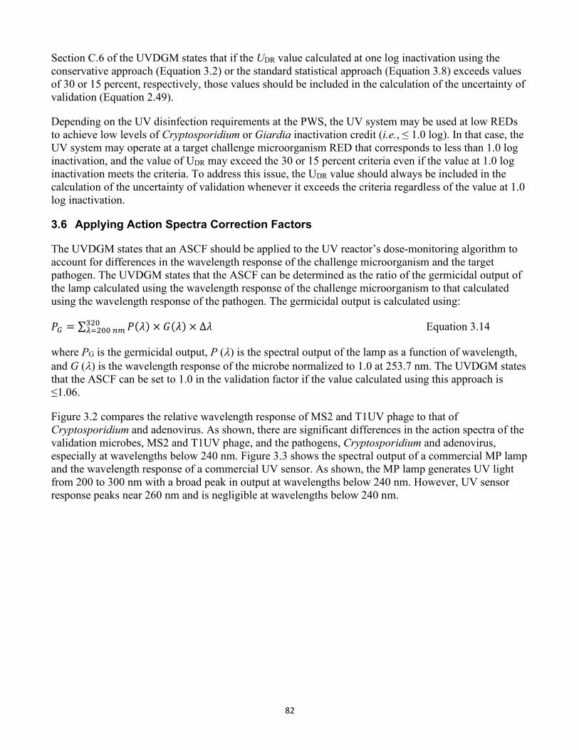
82

Section C.6 of the UVDGM states that if the UDR value calculated at one log inactivation using the conservative approach (Equation 3.2) or the standard statistical approach (Equation 3.8) exceeds values of 30 or 15 percent, respectively, those values should be included in the calculation of the uncertainty of validation (Equation 2.49).

Depending on the UV disinfection requirements at the PWS, the UV system may be used at low REDs to achieve low levels of Cryptosporidium or Giardia inactivation credit (i.e., ≤ 1.0 log). In that case, the UV system may operate at a target challenge microorganism RED that corresponds to less than 1.0 log inactivation, and the value of UDR may exceed the 30 or 15 percent criteria even if the value at 1.0 log inactivation meets the criteria. To address this issue, the UDR value should always be included in the calculation of the uncertainty of validation whenever it exceeds the criteria regardless of the value at 1.0 log inactivation.

3.6 Applying Action Spectra Correction Factors

The UVDGM states that an ASCF should be applied to the UV reactor’s dose-monitoring algorithm to account for differences in the wavelength response of the challenge microorganism and the target pathogen. The UVDGM states that the ASCF can be determined as the ratio of the germicidal output of the lamp calculated using the wavelength response of the challenge microorganism to that calculated using the wavelength response of the pathogen. The germicidal output is calculated using:

𝑃𝑃𝐺𝐺 = ∑ 𝑃𝑃(𝜆𝜆) × 𝐺𝐺(𝜆𝜆) × ∆𝜆𝜆320𝜆𝜆=200 𝑛𝑛𝑛𝑛 Equation 3.14

where PG is the germicidal output, P (λ) is the spectral output of the lamp as a function of wavelength, and G (λ) is the wavelength response of the microbe normalized to 1.0 at 253.7 nm. The UVDGM states that the ASCF can be set to 1.0 in the validation factor if the value calculated using this approach is ≤1.06.

Figure 3.2 compares the relative wavelength response of MS2 and T1UV phage to that of Cryptosporidium and adenovirus. As shown, there are significant differences in the action spectra of the validation microbes, MS2 and T1UV phage, and the pathogens, Cryptosporidium and adenovirus, especially at wavelengths below 240 nm. Figure 3.3 shows the spectral output of a commercial MP lamp and the wavelength response of a commercial UV sensor. As shown, the MP lamp generates UV light from 200 to 300 nm with a broad peak in output at wavelengths below 240 nm. However, UV sensor response peaks near 260 nm and is negligible at wavelengths below 240 nm.

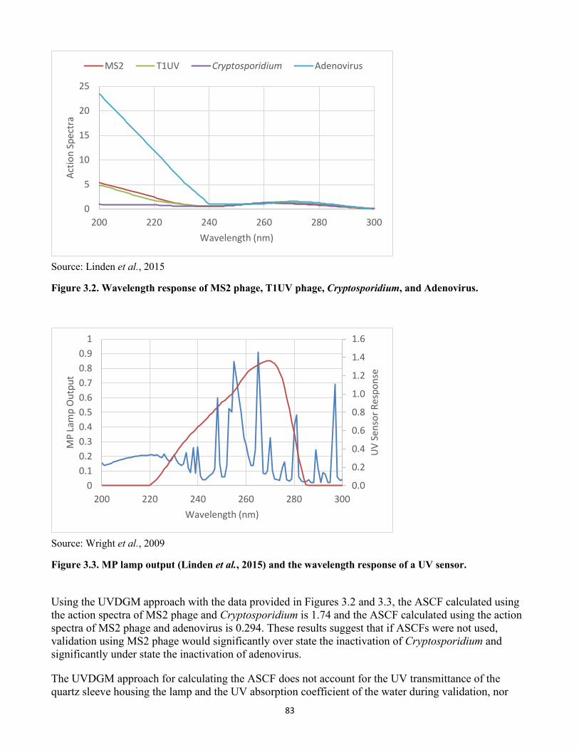
83

0

5

10

15

20

25

200 220 240 260 280 300

Actio

n Sp

ectr

a

Wavelength (nm)

MS2 T1UV Cryptosporidium Adenovirus

Source: Linden et al., 2015

Figure 3.2. Wavelength response of MS2 phage, T1UV phage, Cryptosporidium, and Adenovirus.

0.0

0.2

0.4

0.6

0.8

1.0

1.2

1.4

1.6

00.10.20.30.40.50.60.70.80.9

1

200 220 240 260 280 300

UV

Sens

or R

espo

nse

MP

Lam

p O

utpu

t

Wavelength (nm)

Source: Wright et al., 2009

Figure 3.3. MP lamp output (Linden et al., 2015) and the wavelength response of a UV sensor.

Using the UVDGM approach with the data provided in Figures 3.2 and 3.3, the ASCF calculated using the action spectra of MS2 phage and Cryptosporidium is 1.74 and the ASCF calculated using the action spectra of MS2 phage and adenovirus is 0.294. These results suggest that if ASCFs were not used, validation using MS2 phage would significantly over state the inactivation of Cryptosporidium and significantly under state the inactivation of adenovirus.

The UVDGM approach for calculating the ASCF does not account for the UV transmittance of the quartz sleeve housing the lamp and the UV absorption coefficient of the water during validation, nor

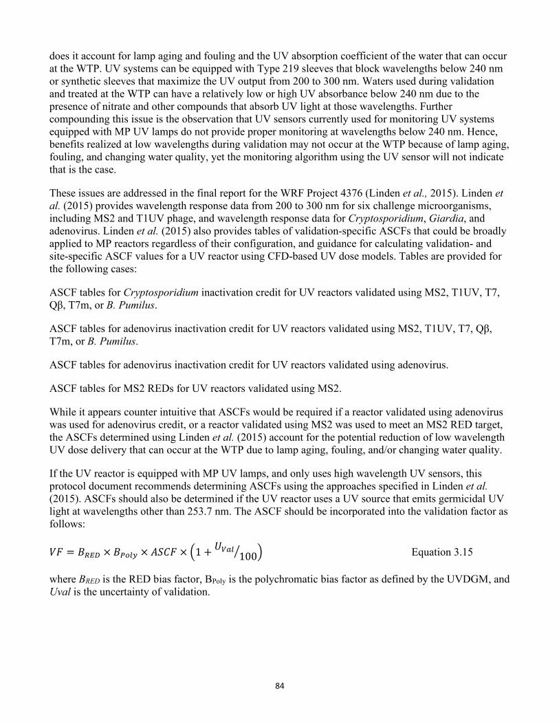
84

does it account for lamp aging and fouling and the UV absorption coefficient of the water that can occur at the WTP. UV systems can be equipped with Type 219 sleeves that block wavelengths below 240 nm or synthetic sleeves that maximize the UV output from 200 to 300 nm. Waters used during validation and treated at the WTP can have a relatively low or high UV absorbance below 240 nm due to the presence of nitrate and other compounds that absorb UV light at those wavelengths. Further compounding this issue is the observation that UV sensors currently used for monitoring UV systems equipped with MP UV lamps do not provide proper monitoring at wavelengths below 240 nm. Hence, benefits realized at low wavelengths during validation may not occur at the WTP because of lamp aging, fouling, and changing water quality, yet the monitoring algorithm using the UV sensor will not indicate that is the case.

These issues are addressed in the final report for the WRF Project 4376 (Linden et al., 2015). Linden et al. (2015) provides wavelength response data from 200 to 300 nm for six challenge microorganisms, including MS2 and T1UV phage, and wavelength response data for Cryptosporidium, Giardia, and adenovirus. Linden et al. (2015) also provides tables of validation-specific ASCFs that could be broadly applied to MP reactors regardless of their configuration, and guidance for calculating validation- and site-specific ASCF values for a UV reactor using CFD-based UV dose models. Tables are provided for the following cases:

ASCF tables for Cryptosporidium inactivation credit for UV reactors validated using MS2, T1UV, T7, Qβ, T7m, or B. Pumilus.

ASCF tables for adenovirus inactivation credit for UV reactors validated using MS2, T1UV, T7, Qβ, T7m, or B. Pumilus.

ASCF tables for adenovirus inactivation credit for UV reactors validated using adenovirus.

ASCF tables for MS2 REDs for UV reactors validated using MS2.

While it appears counter intuitive that ASCFs would be required if a reactor validated using adenovirus was used for adenovirus credit, or a reactor validated using MS2 was used to meet an MS2 RED target, the ASCFs determined using Linden et al. (2015) account for the potential reduction of low wavelength UV dose delivery that can occur at the WTP due to lamp aging, fouling, and/or changing water quality.

If the UV reactor is equipped with MP UV lamps, and only uses high wavelength UV sensors, this protocol document recommends determining ASCFs using the approaches specified in Linden et al. (2015). ASCFs should also be determined if the UV reactor uses a UV source that emits germicidal UV light at wavelengths other than 253.7 nm. The ASCF should be incorporated into the validation factor as follows:

𝑉𝑉𝑉𝑉 = 𝐵𝐵𝑅𝑅𝑅𝑅𝑅𝑅 × 𝐵𝐵𝑃𝑃𝑃𝑃𝑃𝑃𝑃𝑃 × 𝐴𝐴𝑆𝑆𝐴𝐴𝑉𝑉 × �1 + 𝑈𝑈𝑈𝑈𝑎𝑎𝑃𝑃100� � Equation 3.15

where BRED is the RED bias factor, BPoly is the polychromatic bias factor as defined by the UVDGM, and Uval is the uncertainty of validation.

85

3.7 Duty UV Sensor Calibration

Section 6.4.1.1 of the UVDGM describes the use of reference UV sensors to check the calibration of duty UV sensors used by the UV reactor. The checks are done at least once per month. The UVDGM states that the duty UV sensor should be replaced if the ratio of the duty UV sensor reading to the reference UV sensor readings exceeds 1.20. The UVDGM also states that if a replacement duty UV sensor is not available, a UV sensor correction factor should be applied to the target dose setpoint used by the UV system. The UVDGM states that the UV sensor correction factor is calculated as:

𝑈𝑈𝑉𝑉 𝑆𝑆𝑡𝑡𝑆𝑆𝐷𝐷𝐷𝐷𝑠𝑠 𝐴𝐴𝑉𝑉 = 𝑆𝑆𝐷𝐷𝐷𝐷𝑉𝑉𝐷𝐷𝑆𝑆𝑅𝑅𝑜𝑜𝑅𝑅

− 0.2 Equation 3.16

Implicit in the definition of the correction factor is that the UV system can under dose by 20%, which is a significant error.

To prevent under dosing, this document recommends that the UV sensor correction factor be defined as:

𝑈𝑈𝑉𝑉 𝑆𝑆𝑡𝑡𝑆𝑆𝐷𝐷𝐷𝐷𝑠𝑠 𝐴𝐴𝑉𝑉 = 𝑆𝑆𝐷𝐷𝐷𝐷𝑉𝑉𝐷𝐷𝑆𝑆𝑅𝑅𝑜𝑜𝑅𝑅

Equation 3.17

Typically, the duty UV sensor generates 4 to 20 mA or a voltage output that is proportional to the UV intensity measured by the UV sensor. The UV system PLC is programmed with a UV sensor scaling factor that converts the UV sensor's mA or voltage output to a UV intensity in W/m2 or mW/cm2. As an alternate to applying the UV sensor correction factor to the required UV dose, this protocol document recommends adjusting the UV sensor scaling factor using:

𝑓𝑓′ = 𝑓𝑓 × 𝑆𝑆𝑅𝑅𝑜𝑜𝑅𝑅𝑆𝑆𝐷𝐷𝐷𝐷𝑉𝑉𝐷𝐷

Equation 3.18

where f is the scaling factor used by the PLC prior to checking the duty UV sensors, and f' is the new scaling factor based on the comparison of the reference and duty UV sensor readings.

This approach provides a field calibration of the duty UV sensors based on the reference UV sensors, as recommended by Wright et al. (2009). To provide accurate UV dose monitoring, the scaling factor can be adjusted with each comparison of the duty UV sensor with the reference UV sensor, and should be adjusted if the duty sensor signal differs from the reference sensor signal by the UVDGM criteria of >20%.. Adjustments should be performed by qualified personnel only, and should be documented, including the date, the measured values of the duty UV sensor before and after the adjustment, the reference UV sensor values, and the deviation from the nominal manufacturer scaling factor after adjustment.

This on-site adjustment of the scaling factor assumes no significant changes in the spectral response, angular response, or linearity of the UV sensor. To prevent the use of duty UV sensors with large errors related to these changes, the duty UV sensor should be replaced if the adjusted scaling factor deviates by more than 30 percent from the original factory scaling factor for the duty sensor, as recommended by Wright et al. (2009).

86

3.8 Online UVT Monitor QA/QC Criteria

Section 6.4.1.2 of the UVDGM states that the on-line UVT monitors should be evaluated at least once per week by comparing the online UVT measurements to UVT measurements using a bench-top or handheld spectrophotometer. The UVT monitors should be calibrated if the differences between the two measurements exceed two percent.

An error in the online UVT reading has two impacts on UV dose monitoring using the calculated dose approach. First, the error impacts the UVT or UVA used in the UV dose monitoring equation. Second, the error impacts the calculation of S0 used to define the relative lamp output, which in turn is used in the UV dose monitoring equation. The magnitude of the error depends on the reactor and the UVT, and can be determined using the UV dose monitoring algorithm. With some reactors, the error in UV dose monitoring associated with a 2 percent UVT error is on the order of a few percent and can be ignored. With other reactors, the error in UV dose monitoring at high UVTs can range up to 50 percent. As such, the magnitude of the error should be quantified over the validated range of UVT using the UV dose monitoring algorithm given in the validation report. The evaluation should be used to define criteria for the UVT monitor that limits the UV dose monitoring error to at most 10 percent. The accuracy of online UVT monitors at high UVTs can be minimized by using an online monitor with a long optical path length.

3.9 Lamp-to-Lamp Variability

Section 6.3.2.2 of the UVDGM recommends that if the UV reactor used at a WTP does not use one UV sensor per lamp (i.e., the reactor is equipped with more lamps than UV sensors), the WTP should evaluate lamp variability every 2 months with MP UV systems and every 3 months with LP or LPHO systems, and place the lamp with the lowest output with a given group of lamps closest to the UV sensor monitoring that group of lamps. The UVDGM states that if the lamps in a group being monitored by a single UV sensor are close in age (i.e., their age varies by less than 20 percent), it is not necessary to check the lamp output variability. In this case, the oldest lamp should be placed in the position nearest the UV sensor. However, because lamp output decreases with lamp age, if the oldest lamp within a bank of lamps is being monitored, it is not necessary to check the lamp output variability even though the lamp age within that group of lamps varies by 20 percent or more.

3.10 T-Statistics

Sections 5.9.2.1, 5.9.2.2, and B.1.4.1 of the UVDGM give approaches for calculating the uncertainty of the UV intensity setpoint (USP), the uncertainty of interpolation (UIN), and the uncertainty of the UV dose-response (UDR), respectively. The uncertainties are calculated at a 95-percent confidence interval using t-statistics that are provided in the UVDGM as a function of the number of samples. The t-statistics should be defined as a function of the number of samples minus the degrees of freedom. With the uncertainty of the UV intensity setpoint, the degrees of freedom equal 1.0. With the uncertainty of interpolation, the degrees of freedom equal the number of coefficients used in the algorithm used to predict the log inactivation and RED. For example, with Equation 2.56, the degrees of freedom equal 5. With the uncertainty of the UV dose-response, the degrees of freedom equal the number of coefficients in the equation used to fit the UV dose-response of the challenge microorganism. Table 3.3 tabulates the t-statistics as a function of the sample size minus the degrees of freedom.

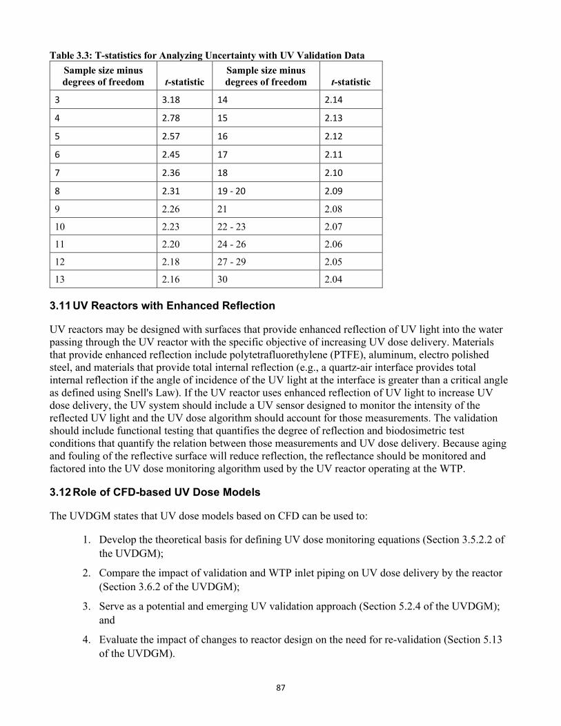
87

Table 3.3: T-statistics for Analyzing Uncertainty with UV Validation Data Sample size minus degrees of freedom t-statistic

Sample size minus degrees of freedom t-statistic

3 3.18 14 2.14

4 2.78 15 2.13

5 2.57 16 2.12

6 2.45 17 2.11

7 2.36 18 2.10

8 2.31 19 - 20 2.09

9 2.26 21 2.08

10 2.23 22 - 23 2.07

11 2.20 24 - 26 2.06

12 2.18 27 - 29 2.05

13 2.16 30 2.04

3.11 UV Reactors with Enhanced Reflection

UV reactors may be designed with surfaces that provide enhanced reflection of UV light into the water passing through the UV reactor with the specific objective of increasing UV dose delivery. Materials that provide enhanced reflection include polytetrafluorethylene (PTFE), aluminum, electro polished steel, and materials that provide total internal reflection (e.g., a quartz-air interface provides total internal reflection if the angle of incidence of the UV light at the interface is greater than a critical angle as defined using Snell's Law). If the UV reactor uses enhanced reflection of UV light to increase UV dose delivery, the UV system should include a UV sensor designed to monitor the intensity of the reflected UV light and the UV dose algorithm should account for those measurements. The validation should include functional testing that quantifies the degree of reflection and biodosimetric test conditions that quantify the relation between those measurements and UV dose delivery. Because aging and fouling of the reflective surface will reduce reflection, the reflectance should be monitored and factored into the UV dose monitoring algorithm used by the UV reactor operating at the WTP.

3.12 Role of CFD-based UV Dose Models

The UVDGM states that UV dose models based on CFD can be used to:

1. Develop the theoretical basis for defining UV dose monitoring equations (Section 3.5.2.2 of the UVDGM);

2. Compare the impact of validation and WTP inlet piping on UV dose delivery by the reactor (Section 3.6.2 of the UVDGM);

3. Serve as a potential and emerging UV validation approach (Section 5.2.4 of the UVDGM); and

4. Evaluate the impact of changes to reactor design on the need for re-validation (Section 5.13 of the UVDGM).

88

Section D.6 of the UVDGM provides approaches and guidelines for developing and using CFD-based UV dose models.

Since the UVDGM was published, the WRF has funded several projects that have developed and used CFD-based UV dose models as a tool for assessing UV reactor performance. Linden et al. (2015) provides guidance for using CFD-based UV dose models to determine ASCFs, and provides an approach for model validation. Important guidance for model validation includes:

1. Develop a geometric model for the reactor including all wetted dimensions of reactor, upstream piping for at least 10 pipe diameters, and downstream piping for at least 5 pipe diameters.

2. Using CFD software, predict the hydraulics and trajectories of virtual microbes through the UV reactor.

3. Calibrate the lamp output used in the UV intensity model by adjusting lamp UV output to give a one-to-one relationship between UV sensor readings measured during validation of the UV reactor and UV sensor readings predicted by the model.

4. Predict log inactivation and RED for each validation test condition using the predicted microbe trajectories, germicidal UV intensity fields, and microbe inactivation kinetics.

5. As QA/QC, verify that the predicted log inactivation or RED is independent of the mesh density used with the geometric model, independent of the convergence of the hydraulic model and the number of particle trajectories.

6. Validate the model by comparing log inactivation or RED predicted by validation to log inactivation or RED predicted by the CFD-based UV dose model. With the lamp output calibrated by comparison of measured and predicted UV sensor readings, the model should predict the full validation dataset (log I or RED) with a slope within 20 percent of 1.0.

7. If the validated model meets the QA/QC criteria in Step 6, fine tune model calibration by adjusting lamp output to give a one-to-one relationship between validation and CFD predicted log inactivation or RED. The final model should predict the full validation dataset (log I or RED) with a slope within 5 percent of 1.00 and an R-squared within 5 percent of the R-squared for the UV dose monitoring algorithm developed through validation.

WRF Project 4478 (Wright and Linden, 2017), entitled "Validation and Site Specific Action Spectra Correction Factors for Medium Pressure Ultraviolet Disinfection Systems," compared log inactivation predicted using CFD-based UV dose models to log inactivation measured during UV validation with six commercial UV reactors equipped with MP UV lamps. Because several of the reactors operated with different numbers of lamps, 19 lamp configurations were modeled. With the model calibrated based on UV sensor readings, the slopes of the relationships between measured and predicted log inactivation ranged from 0.85 to 1.26. However, the R-squared values of the relationships were greater than 0.95 with 14 configurations and greater than 0.92 with 18 of the configurations.

The analysis suggests that the accuracy of CFD-based UV dose models calibrated using UV sensor readings can be ± 26 percent. The cause of these differences was not identified. The analysis suggests that CFD-based UV dose models should not be used as a replacement for biodosimetric validation. However, the high R-squared values suggest that CFD-based UV dose models are a good tool for

89

predicting the relative impacts of flow, water and sleeve UV transmittance, and lamp output. In summary, this protocol document recommends using CFD-based UV dose models to:

1. Develop validation test plans.

2. Evaluate the spectral response of a low wavelength UV sensor within a UV dose algorithm.

3. Evaluate the impact of inlet piping on UV dose delivery.

4. Evaluate minor changes in reactor design on UV dose delivery.

5. Develop ASCF values specific to the UV reactor and its validation.

90

4.0 Microbial Methods Appendix A of the UVDGM gives methods for preparing stock solutions of MS2 phage and B. subtilis spores and enumerating their concentration in water samples collected during UV validation. This section provides methods for preparing stock solutions of alternate UV challenge microorganisms, including numerous phage and B. pumilus spores, and enumerating their concentration in water samples collected during UV validation. The section also provides recommendations for selecting challenge microorganisms, measuring the UV dose-response, and QA/QC bounds for the UV dose-response of MS2 and T1UV phage.


4.1. Selecting Challenge Microorganisms.

4.2. Preparation of Concentrated Bacteriophage.

4.3. Enumeration of Bacteriophage.

4.4. Preparation of Concentrated B. pumilus Spores.

4.5. Enumeration of B. pumilus Spores.

4.6. UV Dose Response QA/QC.

4.1 Selecting Challenge Microorganisms

The UVDGM states that the ideal challenge microorganism has the same UV dose-response and action spectrum as the target pathogen. In practice, the UV dose-response and action spectra of commonly used challenge microorganisms, such as MS2 and B. subtilis spores, differ from that of the target pathogen. To address these differences, the UVDGM recommends applying RED bias factors to account for differences in UV dose response at 254 nm, and, with MP UV reactor, ASCFs to account for differences in wavelength response.

Appendix G of the UVDGM provides RED bias factors as a function of the target pathogen log inactivation, the challenge microorganism UV sensitivity, and the UVT of the water. These factors were determined by analyzing the UV dose delivery of a range of commercial UV reactors using CFD-based UV dose models. The RED bias factors were defined by the analysis on the commercial UV reactor that gave the highest values. With many commercial UV reactors, the true RED bias factors are lower than the values given in the UVDGM, while with a few reactors, the values are somewhat higher. To provide the most efficient application of UV technologies, utilities should use approaches that eliminate or minimize RED bias factors.

The UVDGM promotes the use of challenge microorganisms that minimize the RED bias factor by providing a list of potential challenge microorganisms with UV sensitivities that match that of Cryptosporidium and Giardia better than MS2 phage and B. subtilis spores. The UVDGM also provides RED bias factors for those microbes in Appendix G. However, state regulators have been reluctant to accept UV systems implemented based on validation conducted using these challenge microorganisms. They are reluctant because the UVDGM only provides protocols for the growth and enumeration of

91

MS2 phage and B. subtilis spores, there were no published QA/QC bounds for the UV dose response of those microorganisms, and there were no published action spectra.

The UVDGM also states that validation done with two challenge microorganisms that have a UV dose-response that brackets that of the target pathogen can be interpolated as a function of the UV sensitivity to define the RED delivered to the target pathogens, thereby providing a means of setting the RED bias factor to 1.0. In practice, this approach is not feasible with many validations because conditions of flow, UVT, and lamp output that lead to a measureable inactivation of one microbe will lead to inactivation below the detection limit with a second microbe.

Since the UVDGM was published, UV system manufacturers have conducted validation using challenge microorganisms such as Qβ, T1UV, T1, T7, and T7m phage that have a UV sensitivity that matches that of Cryptosporidium and Giardia better than that of MS2 phage. They have also conducted validation using B. pumilus, A. brasiliensis spores and adenovirus that have a UV sensitivity that can demonstrate high UV doses for virus credit and can provide bracketing of the virus UV dose-response. UV system validators have also developed UV dose algorithms that include the UV sensitivity of the challenge microorganism as a variable (Bircher and Wright, 2007), thereby providing a practical approach for interpolating validation data conducted using multiple microbes as a function of the UV sensitivity.

This protocol document recommends using UV dose algorithms that predict log I and RED as a function of the UV dose per log inactivation of the microbe (DL), to provide direct predictions of pathogen log inactivation and RED as opposed to predicting a validation microbe RED and applying a validation factor. As an alternative to directly predicting the log inactivation of the pathogen, this protocol document recommends using challenge microorganisms such as T1UV phage over MS2 phage for showing Cryptosporidium and/or Giardia inactivation credit, because RED bias factors with these microorganisms are notably lower than RED bias factors with MS2 phage.

If the UV dose algorithm uses a combined variable as described in Section 2, bracketing is not required. While bracketing with multiple microbes is not discouraged, the studies conducted for this research demonstrate that bracketing is not necessary with calculated dose approaches that use the combined variable. With this approach, validation conducted with MS2 and T1UV phage can be used to develop UV dose algorithms that directly predict the log inactivation and RED of the target pathogen without the need to apply an RED bias factor.

Challenge microorganisms, such as T7 phage and B. pumilus spores, are often used during validation with MS2 and T1UV phage to bracket the UV dose-response of the target pathogens. These challenge microorganisms can have a UV dose-response that shows greater variability than MS2 and T1UV phage. The variability can increase the uncertainty of validation with the UV dose monitoring algorithm. If the UV dose algorithm uses a combined variable as described in Section 2, these challenge microorganisms are not required.

4.2 Preparation of Concentrated Bacteriophage

This section gives the approach for preparing bacteriophage stock solutions using the bacteriophage and hosts listed in Table 4.1. The stock solutions are expected to have a concentration ranging from 1 × 1010 plaque forming units (PFU)/mL to 2 × 1012 PFU/mL. To prevent cross contamination, the preparation of stock solution should be separated in time and space from the enumeration of water samples collected during UV validation.

92

Procedure:

1. Inoculate 50 mL of sterile tryptic soy broth (TSB) with host bacteria transferred from a colony grown on a nutrient agar plate. Incubate the culture with constant stirring at 35 to 37°C for 18 to 24 hours.

2. Prepare 1 L of sterile TSB in a sterile 4 L flask. Add 0.3 g calcium chloride dihydrate and 1 g of glucose prepared in 10 mL of de-ionized water.

3. Transfer 10 mL of the host bacterial culture to the 1 L of sterile TSB and incubate at 35°C with continuous shaking at approximately 100 Hertz.

4. Prepare a 1 mL volume of phage in tri-buffered saline (pH 7.3) to the titer given in Table 4.2.

5. After the 1 L host bacterial culture has incubated for the time needed to obtain a culture in its log growth phase (given in Table 4.2), transfer the 1 mL volume of phage to the 1 L host bacterial culture. Continue to incubate at 35°C for 18 to 24 hours.

6. Centrifuge the phage-host culture at 3,000×G (G = 9.82 m/s2) for 30 minutes at 4°C to remove cellular debris.

7. With phage smaller than 0.05 µm (MS2, ɸX174, Qβ, and T7), filter the supernatant through a 0.45 µm cartridge filter followed by a 0.2 µm cartridge filter. For phage greater than 0.05 µm, filter the supernatant through a 1.2 µm cartridge filter.

8. If multiple volumes of phage stock solution are prepared, combined the volumes to form a single stock solution volume.

9. Assay the concentration of the phage stock solution and measure the UV dose-response. The UV dose-response should fall within expected bounds established by the microbial laboratory.

10. Refrigerate the stock solutions at 4°C and use within six months. Steps 6 to 7 may be repeated to prolong storage.

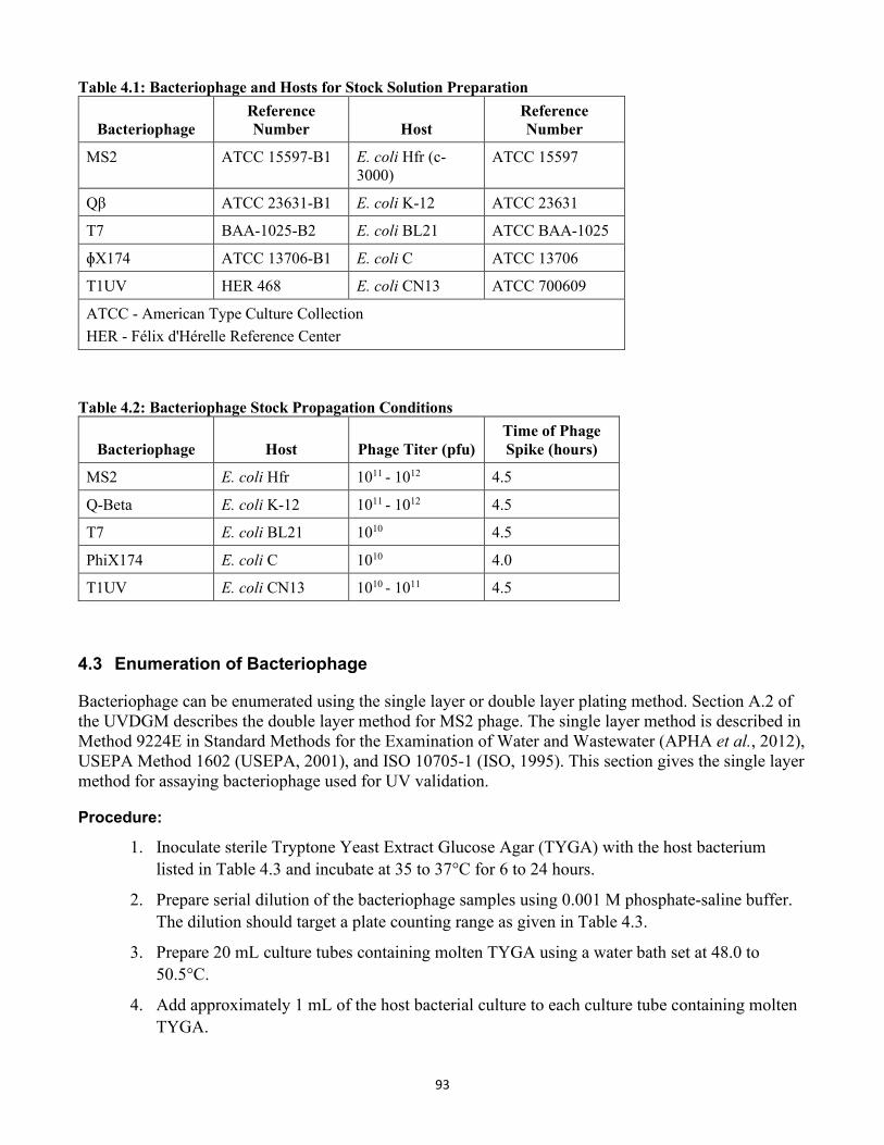
93

Table 4.1: Bacteriophage and Hosts for Stock Solution Preparation

Bacteriophage Reference Number Host

Reference Number

MS2 ATCC 15597-B1 E. coli Hfr (c-3000)

ATCC 15597

Qβ ATCC 23631-B1 E. coli K-12 ATCC 23631

T7 BAA-1025-B2 E. coli BL21 ATCC BAA-1025

ɸX174 ATCC 13706-B1 E. coli C ATCC 13706

T1UV HER 468 E. coli CN13 ATCC 700609

ATCC - American Type Culture Collection HER - Félix d'Hérelle Reference Center

Table 4.2: Bacteriophage Stock Propagation Conditions

Bacteriophage Host Phage Titer (pfu) Time of Phage Spike (hours)

MS2 E. coli Hfr 1011 - 1012 4.5

Q-Beta E. coli K-12 1011 - 1012 4.5

T7 E. coli BL21 1010 4.5

PhiX174 E. coli C 1010 4.0

T1UV E. coli CN13 1010 - 1011 4.5

4.3 Enumeration of Bacteriophage

Bacteriophage can be enumerated using the single layer or double layer plating method. Section A.2 of the UVDGM describes the double layer method for MS2 phage. The single layer method is described in Method 9224E in Standard Methods for the Examination of Water and Wastewater (APHA et al., 2012), USEPA Method 1602 (USEPA, 2001), and ISO 10705-1 (ISO, 1995). This section gives the single layer method for assaying bacteriophage used for UV validation.

Procedure:

1. Inoculate sterile Tryptone Yeast Extract Glucose Agar (TYGA) with the host bacterium listed in Table 4.3 and incubate at 35 to 37°C for 6 to 24 hours.

2. Prepare serial dilution of the bacteriophage samples using 0.001 M phosphate-saline buffer. The dilution should target a plate counting range as given in Table 4.3.

3. Prepare 20 mL culture tubes containing molten TYGA using a water bath set at 48.0 to 50.5°C.

4. Add approximately 1 mL of the host bacterial culture to each culture tube containing molten TYGA.

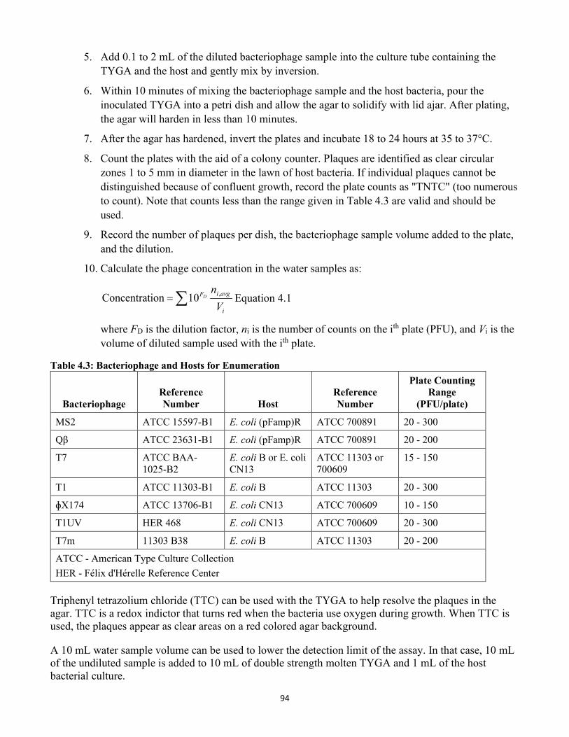
94

5. Add 0.1 to 2 mL of the diluted bacteriophage sample into the culture tube containing the TYGA and the host and gently mix by inversion.

6. Within 10 minutes of mixing the bacteriophage sample and the host bacteria, pour the inoculated TYGA into a petri dish and allow the agar to solidify with lid ajar. After plating, the agar will harden in less than 10 minutes.

7. After the agar has hardened, invert the plates and incubate 18 to 24 hours at 35 to 37°C.

8. Count the plates with the aid of a colony counter. Plaques are identified as clear circular zones 1 to 5 mm in diameter in the lawn of host bacteria. If individual plaques cannot be distinguished because of confluent growth, record the plate counts as "TNTC" (too numerous to count). Note that counts less than the range given in Table 4.3 are valid and should be used.

9. Record the number of plaques per dish, the bacteriophage sample volume added to the plate, and the dilution.

10. Calculate the phage concentration in the water samples as:

∑=i

avgiF

Vn

D ,10ionConcentrat Equation 4.1

where FD is the dilution factor, ni is the number of counts on the ith plate (PFU), and Vi is the volume of diluted sample used with the ith plate.

Table 4.3: Bacteriophage and Hosts for Enumeration

Bacteriophage Reference Number Host

Reference Number

Plate Counting Range

(PFU/plate)

MS2 ATCC 15597-B1 E. coli (pFamp)R ATCC 700891 20 - 300

Qβ ATCC 23631-B1 E. coli (pFamp)R ATCC 700891 20 - 200

T7 ATCC BAA-1025-B2

E. coli B or E. coli CN13

ATCC 11303 or 700609

15 - 150

T1 ATCC 11303-B1 E. coli B ATCC 11303 20 - 300

ɸX174 ATCC 13706-B1 E. coli CN13 ATCC 700609 10 - 150

T1UV HER 468 E. coli CN13 ATCC 700609 20 - 300

T7m 11303 B38 E. coli B ATCC 11303 20 - 200

ATCC - American Type Culture Collection HER - Félix d'Hérelle Reference Center

Triphenyl tetrazolium chloride (TTC) can be used with the TYGA to help resolve the plaques in the agar. TTC is a redox indictor that turns red when the bacteria use oxygen during growth. When TTC is used, the plaques appear as clear areas on a red colored agar background.

A 10 mL water sample volume can be used to lower the detection limit of the assay. In that case, 10 mL of the undiluted sample is added to 10 mL of double strength molten TYGA and 1 mL of the host bacterial culture.

95

Care should be taken to prevent cross contamination of samples. Negative and positive controls should be used as QA/QC.

4.4 Preparation of Concentrated B. pumilus Spores

This section gives the approach for preparing B. pumilus spore stock solutions. To avoid cross contamination, the preparation of stock solution should be separated from the enumeration of water samples collected during UV validation. The UV dose-response of the resulting spores will depend on how the spores are prepared (Rochelle et al., 2010).

Procedure:

1. Prepare 1 liter (L) of tryptic soy agar (TSA) and adjust the pH to 7.3 ± 0.2. Autoclave for 15 minutes at 121°C.

2. Prepare 4 L of Nutrient Agar and supplement with 0.1 mM of MnSO4·H2O. Adjust pH to 6.8 ± 0.2 and autoclave for 15 min at 121°C. Pour into Petri dishes. The MnSO4·H2O concentration can be adjusted to produce spores with a desired sensitivity to UV irradiation.

3. Inoculate Tryptic Soy Agar (Step 1) plates with three smears of B. pumilus and incubate for 24 hours at 37°C.

4. Scrape the B. pumilus cells off the surface of the Tryptic Soy Agar plate and re-suspend in 100mL of Butterfield’s Buffer.

5. Inoculate the Nutrient Agar plates (Step 2) with 100-500 µL of the B. pumilus cell suspension onto each plate.

6. Incubate the inoculated plates for 72 hours at 37°C.

7. Scrape the cells off the surface of the Nutrient Agar plates and filter through cheese cloth to remove any agar that may have been scraped off the plates with the cells. Dilute the filtered cells with phosphate buffered saline to 1 liter (L).

8. Wash the cells by centrifuging the diluted cells at 3,000 × G for 30 minutes at 4°C.

9. Discard supernatant and re-suspend in fresh phosphate buffered saline.

10. Repeat Steps 8 and 9 for two additional wash cycles and re-suspend the cells in 200mL of Butterfield’s Buffer after the final centrifuge cycle.

11. Inactivate the vegetative B. pumilus by heating at 80 ºC for 10 minutes.

12. Collect the resulting stock solution and assay the B. pumilus spore concentration.

13. Refrigerate at 4°C and use within six months.

4.5 Enumeration of B. pumilus Spores

The concentration of B. pumilus spores in water samples can be assayed using plate count agar.

Procedure:

1. Prepare 1 L of TSA with 2.5% NaCl supplemented to the media. Adjust the pH to 7.3 ± 0.2 and autoclave for 15 minutes at 121 º C.

96

2. Obtain serial dilutions of the B. pumilus spore sample using 0.001-M phosphate-saline buffer.

3. Vacuum filter up to 100 mL of diluted or undiluted sample through a 47-mm 0.45-μm membrane filter.

4. Place the filter on a petri dish containing hardened agar and cover plates.

5. Incubate plates un-humidified at 24 ± 2 hours at 37 ± 1 ºC.

6. Count the number of colonies formed with the aid of a colony counter. If individual colonies cannot be distinguished because of confluent growth, record the plate counts as TNTC. The ideal counting range is 20-80 colony forming units (CFU). Counts up to 200 CFU are acceptable.

7. Record the number of colonies per dish, and the B. pumilus spore sample volume and dilution.

8. Calculate the B. pumilus spore concentration in the original samples in units of CFU/mL using:

𝐴𝐴𝐷𝐷𝑆𝑆𝑐𝑐𝑡𝑡𝑆𝑆𝑡𝑡𝑠𝑠𝑉𝑉𝑡𝑡𝑉𝑉𝐷𝐷𝑆𝑆 = ∑10𝐹𝐹𝐷𝐷 × 𝑛𝑛𝑉𝑉,𝑉𝑉𝑎𝑎𝑜𝑜Equation 4.2 𝑈𝑈𝑉𝑉

where FD is the dilution factor, ni is the number of counts on the ith plate (CFU), and Vi is the volume of diluted sample used with the ith plate.

4.6 UV Dose Response QA/QC

Sections A.1 and A.3 of the UVDGM provide figures for the UV dose-response of MS2 and B. subtilis spores as reported in the literature, along with 90th percentile prediction intervals for that dose-response. Those prediction intervals are not meant to be treated as QA/QC criteria because the range of log inactivation with a given UV dose is relatively wide. Instead, Section C.2.4 provides QA/QC criteria for the calculation of UV dose delivered by the collimated beam and Section 5.6.4 of the UVDGM provides criteria for stability of microbial samples collected during validation. An underlying assumption of this approach is that if the microbial samples are stable and the UV dose delivered by the collimated beam apparatus is accurate, the measured UV dose-response will be accurate. However, the UV dose-response of challenge microorganisms, such as MS2 phage, can be impacted by the water matrix and vary over time.

Wright (2018) observed that the UV dose-response of MS2 phage in a collimated beam samples collected during validation can show instability over time and differ from the UV dose-response of the reactor samples passing through the UV reactor. Verhoeven et al. (2017) reported different UV dose-responses with MS2 phage with validation conducted using LSA and SuperHume®. Fallon et al. (2007) reported a degradation of MS2 concentrations with LSA but no degradation with SuperHume®. Thompson and Yates (1999) reports that phage degradation depends on the hydrophobicity of the phage, the ionic strength and concentration of surface active compounds in the solution, and the presence of a dynamic air-water-solid interface where the solid is hydrophobic (such as a container). For these reasons, QA/QC bounds are needed for UV dose-response challenge microorganisms such as the MS2 and T1UV phage.

UV dose-response data for MS2, T1UV, and T7 phage was obtained from a microbial laboratory that specializes in UV validation. Table 4.4 summarizes the number of UV dose-response curves and the

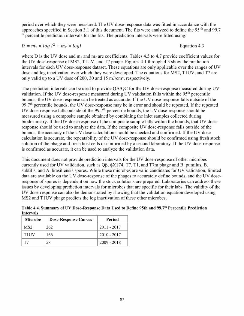
97

period over which they were measured. The UV dose-response data was fitted in accordance with the approaches specified in Section 3.1 of this document. The fits were analyzed to define the 95 th and 99.7

th percentile prediction intervals for the fits. The prediction intervals were fitted using:

𝐷𝐷 = 𝑚𝑚1 × 𝑉𝑉𝐷𝐷𝑙𝑙 𝐼𝐼2 + 𝑚𝑚2 × 𝑉𝑉𝐷𝐷𝑙𝑙𝐼𝐼 Equation 4.3

where D is the UV dose and m1 and m2 are coefficients. Tables 4.5 to 4.7 provide coefficient values for the UV dose-response of MS2, T1UV, and T7 phage. Figures 4.1 through 4.3 show the prediction intervals for each UV dose-response dataset. These equations are only applicable over the ranges of UV dose and log inactivation over which they were developed. The equations for MS2, T1UV, and T7 are only valid up to a UV dose of 200, 30 and 15 mJ/cm2, respectively.

The prediction intervals can be used to provide QA/QC for the UV dose-response measured during UV validation. If the UV dose-response measured during UV validation falls within the 95th percentile bounds, the UV dose-response can be treated as accurate. If the UV dose-response falls outside of the 99.7th percentile bounds, the UV dose-response may be in error and should be repeated. If the repeated UV dose-response falls outside of the 99.7th percentile bounds, the UV dose-response should be measured using a composite sample obtained by combining the inlet samples collected during biodosimetry. If the UV dose-response of the composite sample falls within the bounds, that UV dose-response should be used to analyze the data. If the composite UV dose-response falls outside of the bounds, the accuracy of the UV dose calculation should be checked and confirmed. If the UV dose calculation is accurate, the repeatability of the UV dose-response should be confirmed using fresh stock solution of the phage and fresh host cells or confirmed by a second laboratory. If the UV dose-response is confirmed as accurate, it can be used to analyze the validation data.

This document does not provide prediction intervals for the UV dose-response of other microbes currently used for UV validation, such as Qβ, ɸX174, T7, T1, and T7m phage and B. pumilus, B. subtilis, and A. brasiliensis spores. While these microbes are valid candidates for UV validation, limited data are available on the UV dose-response of the phages to accurately define bounds, and the UV dose-response of spores is dependent on how the stock solutions are prepared. Laboratories can address these issues by developing prediction intervals for microbes that are specific for their labs. The validity of the UV dose-response can also be demonstrated by showing that the validation equation developed using MS2 and T1UV phage predicts the log inactivation of these other microbes.

Table 4.4. Summary of UV Dose-Response Data Used to Define 95th and 99.7th Percentile Prediction Intervals

Microbe Dose-Response Curves Period

MS2 262 2011 - 2017

T1UV 166 2010 - 2017

T7 58 2009 - 2018

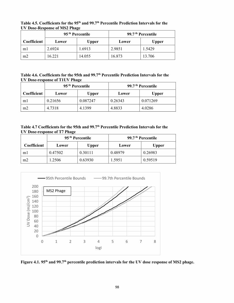
98

Table 4.5. Coefficients for the 95th and 99.7th Percentile Prediction Intervals for the UV Dose-Response of MS2 Phage

Coefficient

95 th Percentile 99.7 th Percentile

Lower Upper Lower Upper

m1 2.6924 1.6913 2.9851 1.5429

m2 16.221 14.055 16.873 13.706

Table 4.6. Coefficients for the 95th and 99.7th Percentile Prediction Intervals for the UV Dose-response of T1UV Phage

Coefficient



m1 0.21656 0.087247 0.26343 0.071269

m2 4.7318 4.1399 4.8833 4.0286

Table 4.7 Coefficients for the 95th and 99.7th Percentile Prediction Intervals for the UV Dose-response of T7 Phage

Coefficient



m1 0.47502 0.30111 0.48979 0.26983

m2 1.2506 0.63930 1.5951 0.59519

Figure 4.1. 95th and 99.7th percentile prediction intervals for the UV dose response of MS2 phage.

020406080

100120140160180200

0 1 2 3 4 5 6 7 8

UV

Dose

(mJ/

cm2 )

logI

95th Percentile Bounds 99.7th Percentile Bounds

MS2 Phage

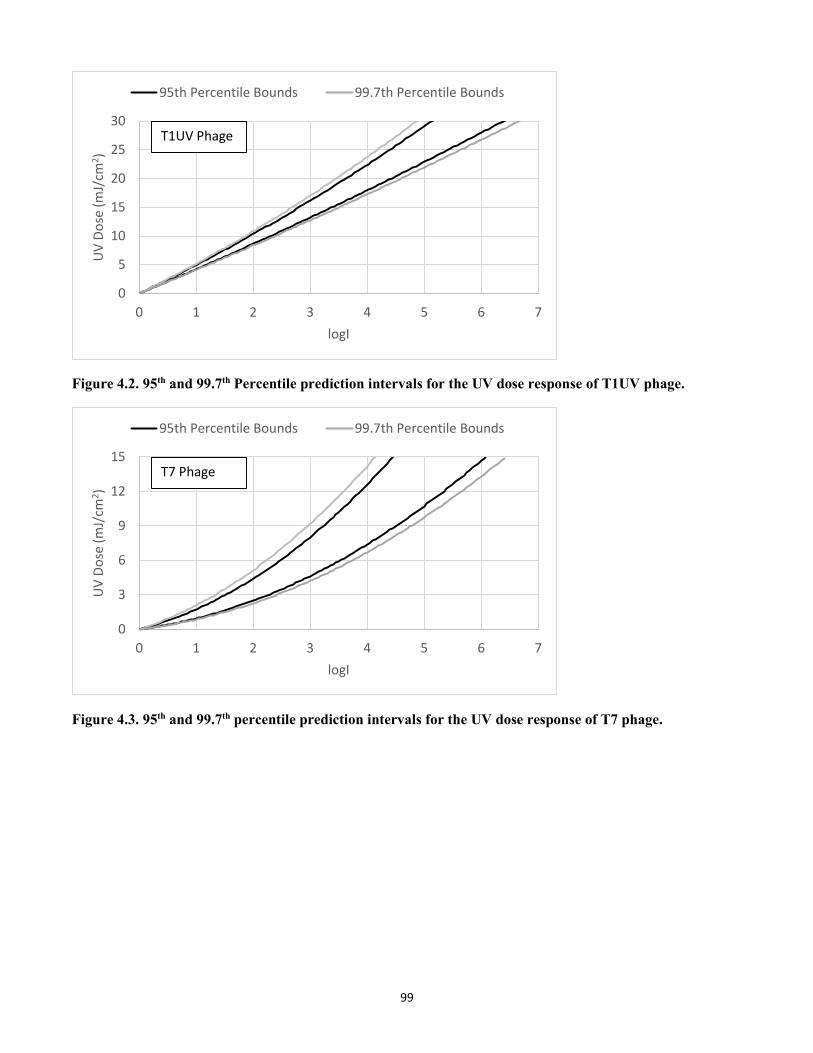
99

0

5

10

15

20

25

30

0 1 2 3 4 5 6 7

UV

Dose

(mJ/

cm2 )

logI


T1UV Phage

Figure 4.2. 95th and 99.7th Percentile prediction intervals for the UV dose response of T1UV phage.

0

3

6

9

12

15

0 1 2 3 4 5 6 7

UV

Dose

(mJ/

cm2 )

logI


T7 Phage

Figure 4.3. 95th and 99.7th percentile prediction intervals for the UV dose response of T7 phage.

100

5.0 Future Research Needs The purpose of this section is to highlight areas for future research associated with the advances presented in this document. Specifically, it identifies seven topics as follows:

1. Reactor/Bank Additivity. While the theory of reactor/bank additivity is well understood from an RED perspective, the implications associated with imperfect mixing between reactor/banks and the impact this has on the combined variable approach needs further investigation, including instances in which multiple banks are added as distinct reactors or are virtually separated within a common shell. Furthermore, in very high-dose applications such as achievement of 6-log virus credit, practical considerations regarding system validation are an issue, especially when the test organisms have relatively low DL values, such as T1 and MS2. Thus, the objective associated with the research would be to enhance the theory of reactor/bank additivity in the context of the combined variable approach and to use the theory to determine appropriate validation guidelines so that validated UV reactor systems can achieve the required 4 to 6 log virus credit. In the future, guidelines need to be developed to address the addition of repeating banks within a single expanded shell beyond the originally validated shell.

2. Using CFD to Complement UV Validation Data. CFD has played an important role in the development of UV reactor performance theory, and was utilized to develop RED bias factors of the UVDGM, as well as to determine ASCF values (Linden et al., 2015). The UVDGM specifically cites that the role of CFD to “serve as a potential and emerging UV validation approach” (Section 5.2.4 of the UVDGM)” and the WRF has funded several projects that have developed and used CFD-based UV dose models as a tool for assessing UV reactor performance (e.g., Ho et al., 2011; Linden et al., 2015). Conclusions from some of these studies suggest that CFD-based models lack the accuracy necessary to be used in place of bioassay validation. Given the cost implications associated with bioassay validation, there is an opportunity to use CFD to complement bioassay data to develop appropriate sizing and monitoring equations. Thus, the objective of this study would be to develop protocols using CFD and bioassay data to provide guidance on how CFD can be used to reduce the full bioassay validation protocol with the specific goal of reducing validation costs, while maintaining the integrity of the sizing and monitoring equations.

3. Extrapolating the Combined Variable Approach on Flow Rate. Currently, no extrapolation on flow rate is allowed when using the combined variable approach. This requirement constrains validated ranges, particularly for achieving high log virus credit at low flow rates (4 or 6 logs). Extrapolation of the flow rate is not recommended because flow patterns through the UV reactor at different flow rates may change significantly outside the validated flow range. The objective of this study would be to investigate the validity of flow rate extrapolation.

4. Polychromatic Sensitivity and Calibration. Research is needed to better define the spectral response of low wavelength UV sensors, define standards for calibration, and understand the long-term performance of these UV sensors. Thus, the objective of this study would be to better define the spectral response of low-wavelength UV sensors, determine appropriate

101

uncertainty bounds for polychromatic systems, and develop and recommend appropriate UV sensor calibration protocols.

5. Surrogates for High UV Doses. UV technologies are an important component of potable reuse trains, being required to obtain 6-log pathogen reduction through disinfection, NDMA reduction through photolysis, and micro pollutant reduction through advanced oxidation. These applications typically involve adenovirus REDs that range upwards of 300 mJ/cm2, and NDMA REDs that range upwards of 600 mJ/cm2. Research is needed to identify surrogates, microbial or otherwise, that can be used to demonstrate these high UV doses.

6. Issues with Reflection. UV light reflection from the walls and other surfaces of a UV reactor can significantly increase UV dose delivery by the reactor, most notably at high UVTs (e.g., greater than 95%). However, the reflection can be reduced over time due to fouling and aging of the reflecting surface. Thus, there is a concern that UV dose algorithms determined during validation could over predict reactor performance in the field. The objective of this study would be to quantify the effect of reactor reflection using both numerical and experimental methods and provide appropriate recommendations for monitoring and validation to address this issue.

7. UV Dose Monitoring and Validation with LEDs. UV reactors that use light emitting diodes (LEDs) as a UV light sources are emerging as a viable option for UV disinfection. Research is needed to define and demonstrate UV dose monitoring and validation for these UV reactors.

102

6.0 References Arnold, W.R. and A.J. Rainbow. 1996. Host cell reactivation of irradiated adenovirus in UV-sensitive

Chinese hamster ovary cell mutants. Mutagenesis, 11(1):89-94.

APHA-AWWA-WEF. 2012. Standard Methods for the Examination of Water and Wastewater, 20th ed. Washington, DC. American Public Health Association, American Water Works Association, Water Environment Federation.

Bircher, K. and H. Wright. 2007. Who needs RED? An empirical method for validating log-inactivation. Presented at the 2007 Water Quality Technology Conference, Charlotte, NC, November 4 to 8, 2007.

Blatchley, E.R., C. Shen, Z. Naunovic, L. Lin, D.A. Lyn, J.P. Robinson, K. Ragheb, G. Grégori, D.E. Bergstrom, S. Fang, Y. Guan, K. Jennings, and N. Gunaratna. 2005. Dyed microspheres for quantification of UV dose distributions: Photochemical reactor characterization by Lagrangian actinometry. Proc. of Disinfection 2005, Sharing Disinfection Technologies: Water, Wastewater, and Biosolids, Mesa, AZ, February 6 to 9, 2005.

Bolton, J.R. 2000. Calculation of ultraviolet fluence rate distributions in an annular reactor: Significance of refraction and reflection. Water Research, 34:3315–3324.

Bolton, J.R. and K.G. Linden. 2003. Standardization of Methods for Fluence (UV Dose) Determination in Bench-Scale UV Experiments. Journal of Environmental Engineering, 129(3):209-216.

Bukhari, Z., T.M. Hargy, J.R. Bolton, B. Dussert, and J.L. Clancy. 1999. Medium Pressure UV Light for Oocyst Inactivation. J. AWWA, 91:86-94.

Cabaj, A., R. Sommer, and D. Schoenen. 1996. Biodosimetry: model calculations for U.V. water disinfection devices with regard to dose distributions. Wat. Res., 30(4):1003-1009.

Craik, S.A., G.R. Finch, J.R. Bolton, and M. Belosevic. 2000. Inactivation of Giardia muris cysts using medium-pressure ultraviolet radiation in filtered drinking water. Water Research, 34(18):4325-4332.

Draper, N., and H. Smith. 1998. Applied Regression Analysis, Third Edition. New York: Wiley.

DVGW. 2006. UV Disinfection Devices for Drinking Water Supply––Requirements and Testing. DVGW W294-1, -2, and -3. German Gas and Water Management Union (DVGW), Bonn, Germany.

Fallon, K.S., T.M. Hargy, E.D. Mackey, H.B. Wright, and J.L. Clancy. 2007. Development and characterization of nonpathogenic surrogates for UV reactor validation. J. Am. Water Works. Assoc., 93(3):73-82.

103

Gerrity, D., H. Ryu, J. Crittenden and M. Abbaszadegan. 2008. UV inactivation of Adenovirus Type 4 measured by integrated cell culture qPCR. Journal of Environmental Science and Health, Part A: Toxic/Hazardous Substances and Environmental Engineering, 43(14):1628-1638.

Ho, C.K., S.S. Khalsa, H.B. Wright, and E. Wicklein. 2011. Computational Fluid Dynamics Based Models for Assessing UV Reactor Design and Installation. Water Research Foundation, Denver, CO.

ISO. 1995. Water quality -- Detection and enumeration of bacteriophages -- Part 1: Enumeration of F-specific RNA bacteriophages. ISO 10705-1:1995. International Organization for Standardization, Geneva, Switzerland.

Jacob, S.M. and J.S. Dranoff. 1970. Light intensity profiles in a perfectly mixed photoreactor. AIChE Journal, 16(3):359-363.

Linden, K.G., H. Wright, J. Collins, C. Cotton, and S.E. Beck. 2015. Guidance for Implementing Action Spectra Correction with Medium Pressure UV Disinfection. Water Research Foundation, Denver, CO.

Mayor-Smith, I. and M.R. Templeton. 2014. Methodological considerations when conducting bench scale polychromatic ultraviolet irradiation of water. Water Science & Technology: Water Supply, 14(2): 291-298.

NIST/SEMATECH. 2012. e-Handbook of Statistical Methods, http://www.itl.nist.gov/div898/handbook/

NWRI and WRF. 2012. Ultraviolet Disinfection Guidelines for Drinking Water and Water Reuse. Third Edition. National Water Research Institute, Fountain Valley, CA, in collaboration with American Water Works Association Research Foundation.

ÖNORM. 2001. Plants for the disinfection of water using ultraviolet radiation—Requirements and testing—Part 1: Low pressure mercury lamp plants. ÖNORM M 5873-1. Osterreichisches Normungsinstitut, Vienna, Austria.

ÖNORM. 2003. Plants for the disinfection of water using ultraviolet radiation—Requirements and testing—Part 2: Medium pressure mercury lamp plants. ÖNORM M 5873-2. Osterreichisches Normungsinstitut, Vienna, Austria.

Paccione J.D., D.M. Dziewulski, and P.L. Young. 2017. Development of recreational water spray ground design regulations in New York State, an engineering approach. J Water Health, 15(5):718-728.

Qian, S.S., M. Donnelly, D.C. Schmelling, M. Messner, K.L. Linden, and C. Cotton. 2004. Ultraviolet light inactivation of protozoa in drinking water: a Bayesian meta-analysis, Wat. Res., 38(2):317-326.

Taylor-Edmonds, L., T. Lichi, A. Rotstein-Mayer and H. Mamane. 2015. The impact of dose, irradiance and growth conditions on Aspergillus niger (renamed A. brasiliensis) spores low-pressure (LP) UV inactivation. J Environ Sci Health A Tox Hazard Subst Environ Eng. 50(4):341-7.

104

Rochelle, P.A., E.R. Blatchley, P.-S. Chan, O.K. Scheible, C. Shen. 2010. Challenge Organisms for Inactivation of Viruses by Ultraviolet Treatment. American Water Works Association Research Foundation, Denver, CO.

Thompson, S.S and M.V. Yates. 1999. Bacteriophage inactivation at the air-water-solid interface in dynamic batch systems. Appl. Environ. Microbiol., 65(3):1186-1190.

USEPA. 2001. Method 1602: Male-specific (F+) and Somatic Coliphage in Water by Single Agar Layer (SAL) Procedure. EPA 821-R-01-029. Office of Water, Washington, DC

USEPA. 2003. Ultraviolet Disinfection Guidance Manual. EPA 815-D-03-007. U.S. Environmental Protection Agency, Office of Groundwater and Drinking Water, Washington, DC.

USEPA. 2006. Ultraviolet Disinfection Guidance Manual for The Final Long Term 2 Enhanced Surface Water Treatment Rule. EPA 815-R-06-007. U.S. Environmental Protection Agency, Office of Groundwater and Drinking Water, Washington, DC.

USPHS/FDA. 2015. Grade “A” Pasteurized Milk Ordinance. U.S. Department of Health and Human Services, Public Health Service, and Food and Drug Administration.

Verhoeven, S. and H. Wright, C. Odegaard, J. Shaw, and K. Bircher. 2011. Reflections cause measureable error when calculating UV dose in a collimated beam apparatus. Proceedings of the IUVA World Congress, May 23 to 27, 2011, Paris, France.

Verhoeven, S., L. Sealey, J. Patterson, and C. Odegaard. 2017. Not all water is created equal: The effects of water characteristics on MS2 stability. Presented at the 2017 IUVA Americas Conference, February 5-8, Austin, Texas.

Wright, H., E.D. Mackey, D. Gaithuma, C. Fonseca, L. Baumberger, T. Dzurny, J. Clancy, T. Hargy, K. Fallon, A. Cabaj, A. Schmalweiser, A. Beirman, and C. Gribbin. 2007. Optimization of UV Disinfection. American Water Works Association Research Foundation, Denver, CO.

Wright, H., D. Gaithuma, T. Dzurny, C. Schulz, K. McCurdy, T. Bogan, A. Cabaj, A. Schmalweisser, Y. Ohno, and T. Larason. 2009. Design and Performance Guidelines for UV Sensor Systems. Water Research Foundation, Denver, CO.

Wright, H., M. Heath, and J. Bandy. 2011a. Yikes! What the UVDGM does not address on UV disinfection. Proceedings of the IUVA World Congress, May 23 to 27, 2011, Paris, France.

Wright, H., M. Heath, J. Bandy, C. Bokermann, and R. Bemus. 2011b. Impact of low wavelength UV light on UV dose monitoring with medium pressure UV systems. Proceedings of the Water Quality Technology Conference and Exposition, November 13 to 17, 2011, Phoenix, Arizona.

Wright, H., D. Gaithuma, M. Heath, C. Schulz, T. Bogan, A. Cabaj, A. Schmalweiser, M. Schmelzer, and J. Finegan-Kelly. 2012. UV Disinfection Knowledge Base. Water Research Foundation, Denver, CO.

Wright, H. (2018). Personnel Communication regarding observed UV dose response at the Portland UV Validation Test Facility.

105

Wright, H and Linden, K.G. 2018. Validation and Site Specific Action Spectra Correction Factors for Medium Pressure UV Disinfection Systems. Water Research Foundation, Denver, CO.

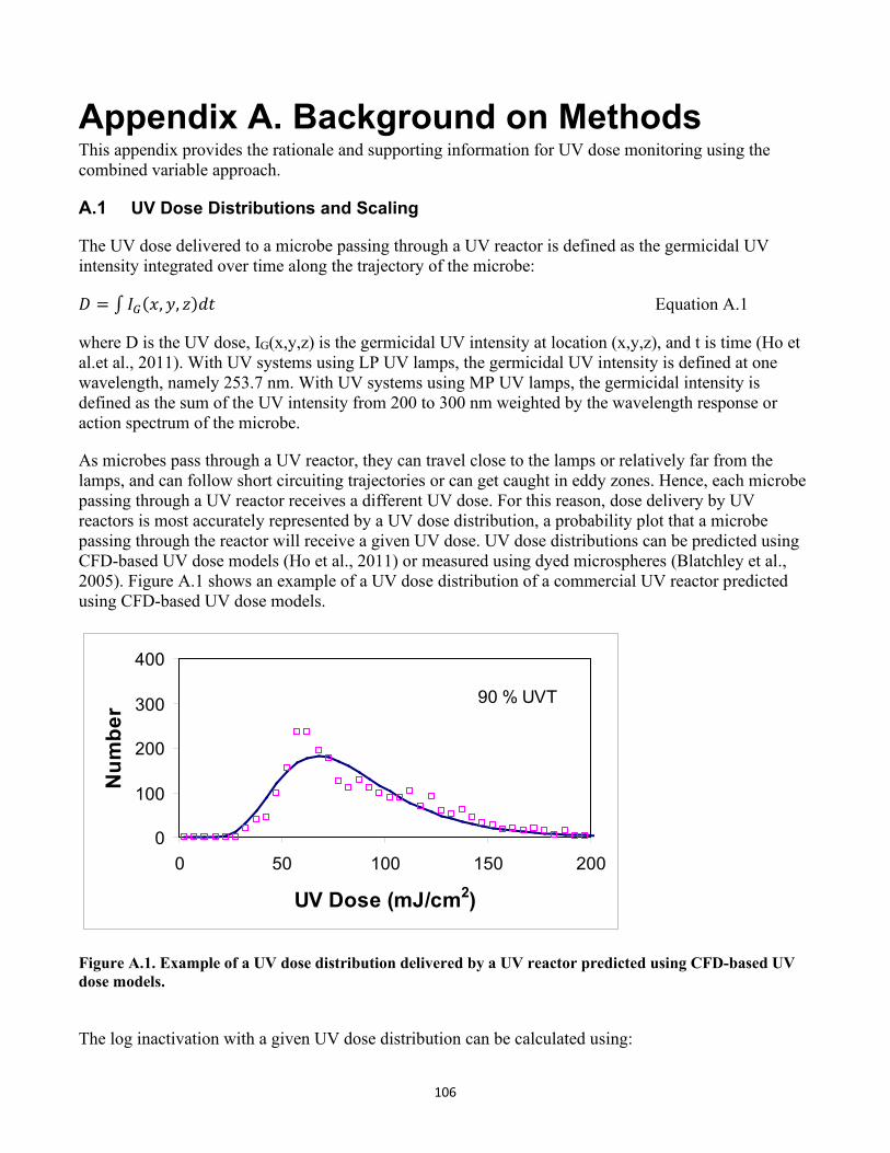
106

Appendix A. Background on Methods This appendix provides the rationale and supporting information for UV dose monitoring using the combined variable approach.

A.1 UV Dose Distributions and Scaling

The UV dose delivered to a microbe passing through a UV reactor is defined as the germicidal UV intensity integrated over time along the trajectory of the microbe:

𝐷𝐷 = ∫ 𝐼𝐼𝐺𝐺(𝑒𝑒,𝑦𝑦, 𝑧𝑧)𝑉𝑉𝑡𝑡 Equation A.1

where D is the UV dose, IG(x,y,z) is the germicidal UV intensity at location (x,y,z), and t is time (Ho et al.et al., 2011). With UV systems using LP UV lamps, the germicidal UV intensity is defined at one wavelength, namely 253.7 nm. With UV systems using MP UV lamps, the germicidal intensity is defined as the sum of the UV intensity from 200 to 300 nm weighted by the wavelength response or action spectrum of the microbe.

As microbes pass through a UV reactor, they can travel close to the lamps or relatively far from the lamps, and can follow short circuiting trajectories or can get caught in eddy zones. Hence, each microbe passing through a UV reactor receives a different UV dose. For this reason, dose delivery by UV reactors is most accurately represented by a UV dose distribution, a probability plot that a microbe passing through the reactor will receive a given UV dose. UV dose distributions can be predicted using CFD-based UV dose models (Ho et al., 2011) or measured using dyed microspheres (Blatchley et al., 2005). Figure A.1 shows an example of a UV dose distribution of a commercial UV reactor predicted using CFD-based UV dose models.

Figure A.1. Example of a UV dose distribution delivered by a UV reactor predicted using CFD-based UV dose models.

The log inactivation with a given UV dose distribution can be calculated using:

0

100

200

300

400

0 50 100 150 200

UV Dose (mJ/cm2)

Num

ber 90 % UVT

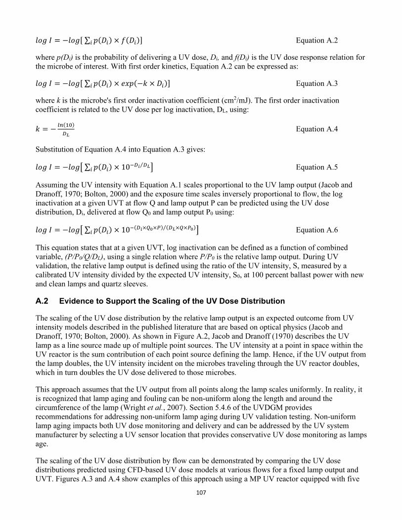
107

𝑉𝑉𝐷𝐷𝑙𝑙 𝐼𝐼 = −𝑉𝑉𝐷𝐷𝑙𝑙[ ∑ 𝑒𝑒(𝐷𝐷𝑀𝑀) × 𝑓𝑓(𝐷𝐷𝑀𝑀)𝑀𝑀 ] Equation A.2

where p(Di) is the probability of delivering a UV dose, Di, and f(Di) is the UV dose response relation for the microbe of interest. With first order kinetics, Equation A.2 can be expressed as:

𝑉𝑉𝐷𝐷𝑙𝑙 𝐼𝐼 = −𝑉𝑉𝐷𝐷𝑙𝑙[ ∑ 𝑒𝑒(𝐷𝐷𝑀𝑀) × 𝑡𝑡𝑒𝑒𝑒𝑒(−𝑘𝑘 × 𝐷𝐷𝑀𝑀)𝑀𝑀 ] Equation A.3

where k is the microbe's first order inactivation coefficient (cm2/mJ). The first order inactivation coefficient is related to the UV dose per log inactivation, DL, using:

𝑘𝑘 = − 𝑃𝑃𝑛𝑛(10)𝑅𝑅𝐿𝐿

Equation A.4

Substitution of Equation A.4 into Equation A.3 gives:

𝑉𝑉𝐷𝐷𝑙𝑙 𝐼𝐼 = −𝑉𝑉𝐷𝐷𝑙𝑙� ∑ 𝑒𝑒(𝐷𝐷𝑀𝑀) × 10−𝑅𝑅𝑉𝑉 𝑅𝑅𝐿𝐿⁄𝑀𝑀 � Equation A.5

Assuming the UV intensity with Equation A.1 scales proportional to the UV lamp output (Jacob and Dranoff, 1970; Bolton, 2000) and the exposure time scales inversely proportional to flow, the log inactivation at a given UVT at flow Q and lamp output P can be predicted using the UV dose distribution, Di, delivered at flow Q0 and lamp output P0 using:

𝑉𝑉𝐷𝐷𝑙𝑙 𝐼𝐼 = −𝑉𝑉𝐷𝐷𝑙𝑙� ∑ 𝑒𝑒(𝐷𝐷𝑀𝑀) × 10−(𝑅𝑅𝑉𝑉×𝑄𝑄0×𝑃𝑃) (𝑅𝑅𝐿𝐿×𝑄𝑄×𝑃𝑃0)⁄𝑀𝑀 � Equation A.6

This equation states that at a given UVT, log inactivation can be defined as a function of combined variable, (P/P0/Q/DL), using a single relation where P/P0 is the relative lamp output. During UV validation, the relative lamp output is defined using the ratio of the UV intensity, S, measured by a calibrated UV intensity divided by the expected UV intensity, S0, at 100 percent ballast power with new and clean lamps and quartz sleeves.

A.2 Evidence to Support the Scaling of the UV Dose Distribution

The scaling of the UV dose distribution by the relative lamp output is an expected outcome from UV intensity models described in the published literature that are based on optical physics (Jacob and Dranoff, 1970; Bolton, 2000). As shown in Figure A.2, Jacob and Dranoff (1970) describes the UV lamp as a line source made up of multiple point sources. The UV intensity at a point in space within the UV reactor is the sum contribution of each point source defining the lamp. Hence, if the UV output from the lamp doubles, the UV intensity incident on the microbes traveling through the UV reactor doubles, which in turn doubles the UV dose delivered to those microbes.

This approach assumes that the UV output from all points along the lamp scales uniformly. In reality, it is recognized that lamp aging and fouling can be non-uniform along the length and around the circumference of the lamp (Wright et al., 2007). Section 5.4.6 of the UVDGM provides recommendations for addressing non-uniform lamp aging during UV validation testing. Non-uniform lamp aging impacts both UV dose monitoring and delivery and can be addressed by the UV system manufacturer by selecting a UV sensor location that provides conservative UV dose monitoring as lamps age.

The scaling of the UV dose distribution by flow can be demonstrated by comparing the UV dose distributions predicted using CFD-based UV dose models at various flows for a fixed lamp output and UVT. Figures A.3 and A.4 show examples of this approach using a MP UV reactor equipped with five

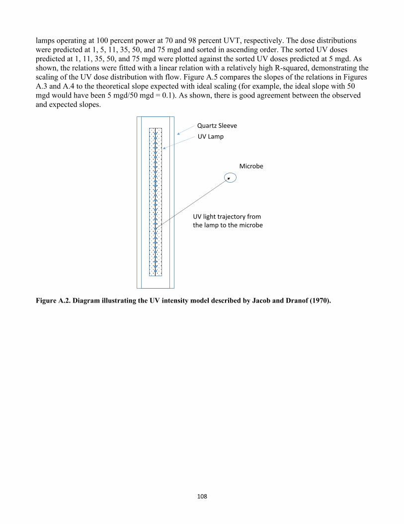
108

lamps operating at 100 percent power at 70 and 98 percent UVT, respectively. The dose distributions were predicted at 1, 5, 11, 35, 50, and 75 mgd and sorted in ascending order. The sorted UV doses predicted at 1, 11, 35, 50, and 75 mgd were plotted against the sorted UV doses predicted at 5 mgd. As shown, the relations were fitted with a linear relation with a relatively high R-squared, demonstrating the scaling of the UV dose distribution with flow. Figure A.5 compares the slopes of the relations in Figures A.3 and A.4 to the theoretical slope expected with ideal scaling (for example, the ideal slope with 50 mgd would have been 5 mgd/50 mgd = 0.1). As shown, there is good agreement between the observed and expected slopes.

Microbe

Quartz SleeveUV Lamp

UV light trajectory fromthe lamp to the microbe

Figure A.2. Diagram illustrating the UV intensity model described by Jacob and Dranof (1970).

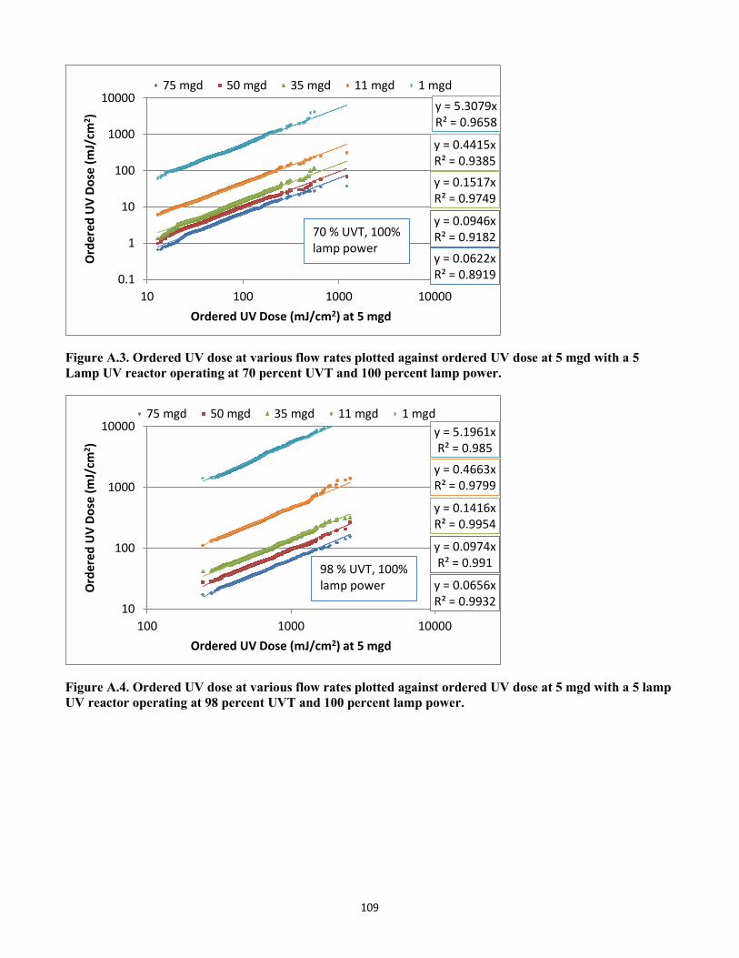
109

y = 0.0622xR² = 0.8919

y = 0.0946xR² = 0.9182

y = 0.1517xR² = 0.9749

y = 0.4415xR² = 0.9385

y = 5.3079xR² = 0.9658

0.1

1

10

100

1000

10000

10 100 1000 10000

Ord

ered

UV

Dose

(mJ/

cm2 )

Ordered UV Dose (mJ/cm2) at 5 mgd

75 mgd 50 mgd 35 mgd 11 mgd 1 mgd

70 % UVT, 100% lamp power

Figure A.3. Ordered UV dose at various flow rates plotted against ordered UV dose at 5 mgd with a 5 Lamp UV reactor operating at 70 percent UVT and 100 percent lamp power.

y = 0.0656xR² = 0.9932

y = 0.0974xR² = 0.991

y = 0.1416xR² = 0.9954

y = 0.4663xR² = 0.9799

y = 5.1961xR² = 0.985

10

100

1000

10000

100 1000 10000

Ord

ered

UV

Dose

(mJ/

cm2 )

Ordered UV Dose (mJ/cm2) at 5 mgd

75 mgd 50 mgd 35 mgd 11 mgd 1 mgd

98 % UVT, 100% lamp power

Figure A.4. Ordered UV dose at various flow rates plotted against ordered UV dose at 5 mgd with a 5 lamp UV reactor operating at 98 percent UVT and 100 percent lamp power.

110

0.01

0.10

1.00

10.00

0.01 0.10 1.00 10.00

Obs

erve

d Sl

ope

Theoretical Slope

98 percent UVT 70 percent UVT 1:1 Relation

Figure A.5. Comparison of observed slopes with Figures A.3 and A.4 with slopes expected with ideal scaling.

The scaling of the UV dose distribution with a given UV reactor can also be demonstrated by comparing the log inactivation measured during validation to that predicted using CFD-based UV dose models where the CFD model is run at one flow rate and used to predict the UV dose distributions at the various UVTs evaluated during validation. Those UV dose distributions are then scaled to the flows and relative lamp outputs used with the validation, and then used to predict the log inactivation using the microbe's UV dose response.

Using this approach, Figure A.6 compares the measured and predicted log inactivation with a MP UV reactor where the UV dose distributions, defined by 1,983 microbe trajectories predicted at 3 mgd, were used to predict log inactivation measured from 3 to 50 mgd at UVTs from 75 to 98 percent and relative lamp outputs from 0.3 to 1.0. As shown by the R-squared value of 0.9813, a single set of microbe trajectories predicted at one flow rate accurately predicted log inactivation over the full validated range of flow and relative lamp output demonstrating that UV dose distributions scale proportionally to the lamp output and inversely proportional to flow. For comparison purposes, the R-squared of the equation used to fit the validation data was 0.9878.

Table A.1 provides further comparisons of log inactivation measured during validation to log inactivation predicted using CFD-based UV dose models where the CFD was run at one flow rate. The comparisons are made with 11 reactor configurations. With a given configuration, the flow rates during validation varied by a factor of 18 to 20 and the relative lamp output varied by a factor of 3.1 to 3.7. The R-squared for the linear relation between measured and CFD-predicted log inactivation ranged from 0.9307 to 0.9869 and was comparable to the range of R-squared for the linear relation between measured and validation equation-predicted log inactivation of 0.9479 to 0.9900. The analysis provides further evidence demonstrating that UV dose distributions scale proportionally to the lamp output and inversely proportional to flow.

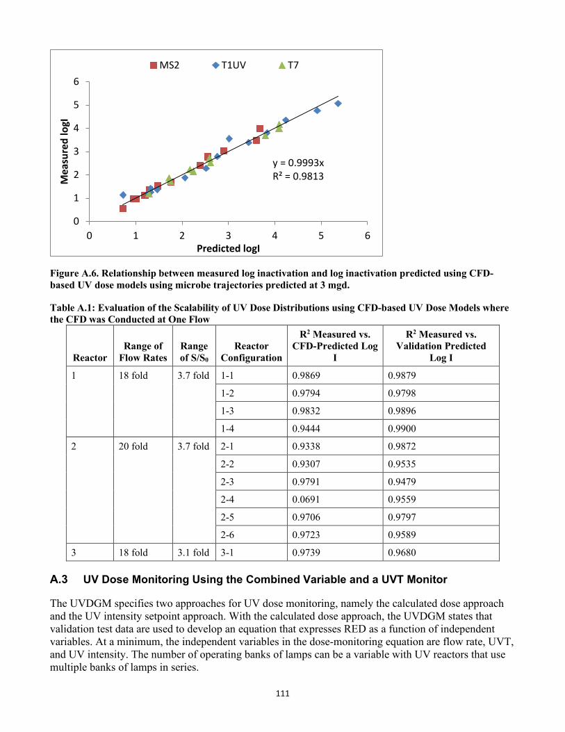
111

y = 0.9993xR² = 0.9813

0

1

2

3

4

5

6

0 1 2 3 4 5 6

Mea

sure

d lo

gI

Predicted logI

MS2 T1UV T7

Figure A.6. Relationship between measured log inactivation and log inactivation predicted using CFD-based UV dose models using microbe trajectories predicted at 3 mgd.

Table A.1: Evaluation of the Scalability of UV Dose Distributions using CFD-based UV Dose Models where the CFD was Conducted at One Flow

Reactor Range of

Flow Rates Range of S/S0

Reactor Configuration

R2 Measured vs. CFD-Predicted Log

I

R2 Measured vs. Validation Predicted

Log I

1 18 fold 3.7 fold 1-1 0.9869 0.9879

1-2 0.9794 0.9798

1-3 0.9832 0.9896

1-4 0.9444 0.9900

2 20 fold 3.7 fold 2-1 0.9338 0.9872

2-2 0.9307 0.9535

2-3 0.9791 0.9479

2-4 0.0691 0.9559

2-5 0.9706 0.9797

2-6 0.9723 0.9589

3 18 fold 3.1 fold 3-1 0.9739 0.9680

A.3 UV Dose Monitoring Using the Combined Variable and a UVT Monitor

The UVDGM specifies two approaches for UV dose monitoring, namely the calculated dose approach and the UV intensity setpoint approach. With the calculated dose approach, the UVDGM states that validation test data are used to develop an equation that expresses RED as a function of independent variables. At a minimum, the independent variables in the dose-monitoring equation are flow rate, UVT, and UV intensity. The number of operating banks of lamps can be a variable with UV reactors that use multiple banks of lamps in series.

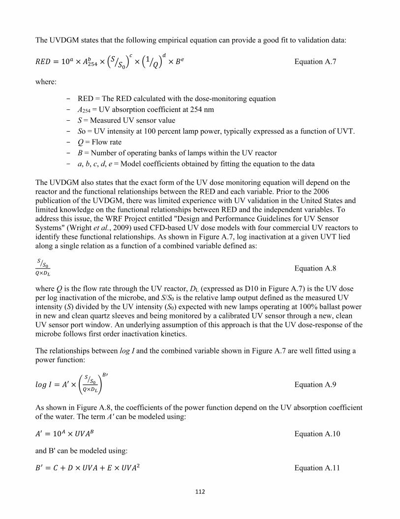
112

The UVDGM states that the following empirical equation can provide a good fit to validation data:

𝑅𝑅𝑅𝑅𝐷𝐷 = 10𝑎𝑎 × 𝐴𝐴254𝑏𝑏 × �𝑆𝑆 𝑆𝑆0� �𝑐𝑐

× �1𝑄𝑄� �

𝑑𝑑× 𝐵𝐵𝑒𝑒

where:

Equation A.7

RED = The RED calculated with the dose-monitoring equation A254 = UV absorption coefficient at 254 nm S = Measured UV sensor value So = UV intensity at 100 percent lamp power, typically expressed as a function of UVT. Q = Flow rate B = Number of operating banks of lamps within the UV reactor a, b, c, d, e = Model coefficients obtained by fitting the equation to the data

The UVDGM also states that the exact form of the UV dose monitoring equation will depend on the reactor and the functional relationships between the RED and each variable. Prior to the 2006 publication of the UVDGM, there was limited experience with UV validation in the United States and limited knowledge on the functional relationships between RED and the independent variables. To address this issue, the WRF Project entitled "Design and Performance Guidelines for UV Sensor Systems" (Wright et al., 2009) used CFD-based UV dose models with four commercial UV reactors to identify these functional relationships. As shown in Figure A.7, log inactivation at a given UVT lied along a single relation as a function of a combined variable defined as:

𝑆𝑆𝑆𝑆0�

𝑄𝑄×𝑅𝑅𝐿𝐿 Equation A.8

where Q is the flow rate through the UV reactor, DL (expressed as D10 in Figure A.7) is the UV dose per log inactivation of the microbe, and S/S0 is the relative lamp output defined as the measured UV intensity (S) divided by the UV intensity (S0) expected with new lamps operating at 100% ballast power in new and clean quartz sleeves and being monitored by a calibrated UV sensor through a new, clean UV sensor port window. An underlying assumption of this approach is that the UV dose-response of the microbe follows first order inactivation kinetics.

The relationships between log I and the combined variable shown in Figure A.7 are well fitted using a power function:



Equation A.9

As shown in Figure A.8, the coefficients of the power function depend on the UV absorption coefficient of the water. The term A' can be modeled using:

𝐴𝐴′ = 10𝐴𝐴 × 𝑈𝑈𝑉𝑉𝐴𝐴𝐵𝐵 Equation A.10

and B' can be modeled using:

𝐵𝐵′ = 𝐴𝐴 + 𝐷𝐷 × 𝑈𝑈𝑉𝑉𝐴𝐴 + 𝑅𝑅 × 𝑈𝑈𝑉𝑉𝐴𝐴2 Equation A.11

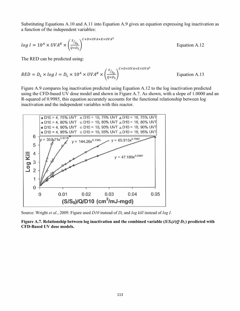
113

Substituting Equations A.10 and A.11 into Equation A.9 gives an equation expressing log inactivation as a function of the independent variables:

𝑉𝑉𝐷𝐷𝑙𝑙 𝐼𝐼 = 10𝐴𝐴 × 𝑈𝑈𝑉𝑉𝐴𝐴𝐵𝐵 × �𝑆𝑆𝑆𝑆0�


Equation A.12

The RED can be predicted using:

𝑅𝑅𝑅𝑅𝐷𝐷 = 𝐷𝐷𝐿𝐿 × 𝑉𝑉𝐷𝐷𝑙𝑙 𝐼𝐼 = 𝐷𝐷𝐿𝐿 × 10𝐴𝐴 × 𝑈𝑈𝑉𝑉𝐴𝐴𝐵𝐵 × �𝑆𝑆𝑆𝑆0�


Equation A.13

Figure A.9 compares log inactivation predicted using Equation A.12 to the log inactivation predicted using the CFD-based UV dose model and shown in Figure A.7. As shown, with a slope of 1.0000 and an R-squared of 0.9985, this equation accurately accounts for the functional relationship between log inactivation and the independent variables with this reactor.

Source: Wright et al., 2009. Figure used D10 instead of DL and log kill instead of log I.

Figure A.7. Relationship between log inactivation and the combined variable (S/S0)/(Q DL) predicted with CFD-Based UV dose models.

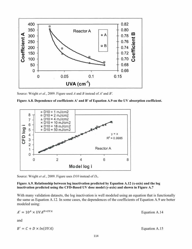
114

Source: Wright et al., 2009. Figure used A and B instead of A' and B'.

Figure A.8. Dependence of coefficients A' and B' of Equation A.9 on the UV absorption coefficient.

Source: Wright et al., 2009. Figure uses D10 instead of DL.

Figure A.9. Relationship between log inactivation predicted by Equation A.12 (x-axis) and the log inactivation predicted using the CFD-Based UV dose model (y-axis) and shown in Figure A.7

With many validation datasets, the log inactivation is well modeled using an equation that is functionally the same as Equation A.12. In some cases, the dependences of the coefficients of Equation A.9 are better modeled using:

𝐴𝐴′ = 10𝐴𝐴 × 𝑈𝑈𝑉𝑉𝐴𝐴𝐵𝐵×𝑈𝑈𝑈𝑈𝐴𝐴 Equation A.14

and

𝐵𝐵′ = 𝐴𝐴 + 𝐷𝐷 × 𝑉𝑉𝑆𝑆(𝑈𝑈𝑉𝑉𝐴𝐴) Equation A.15

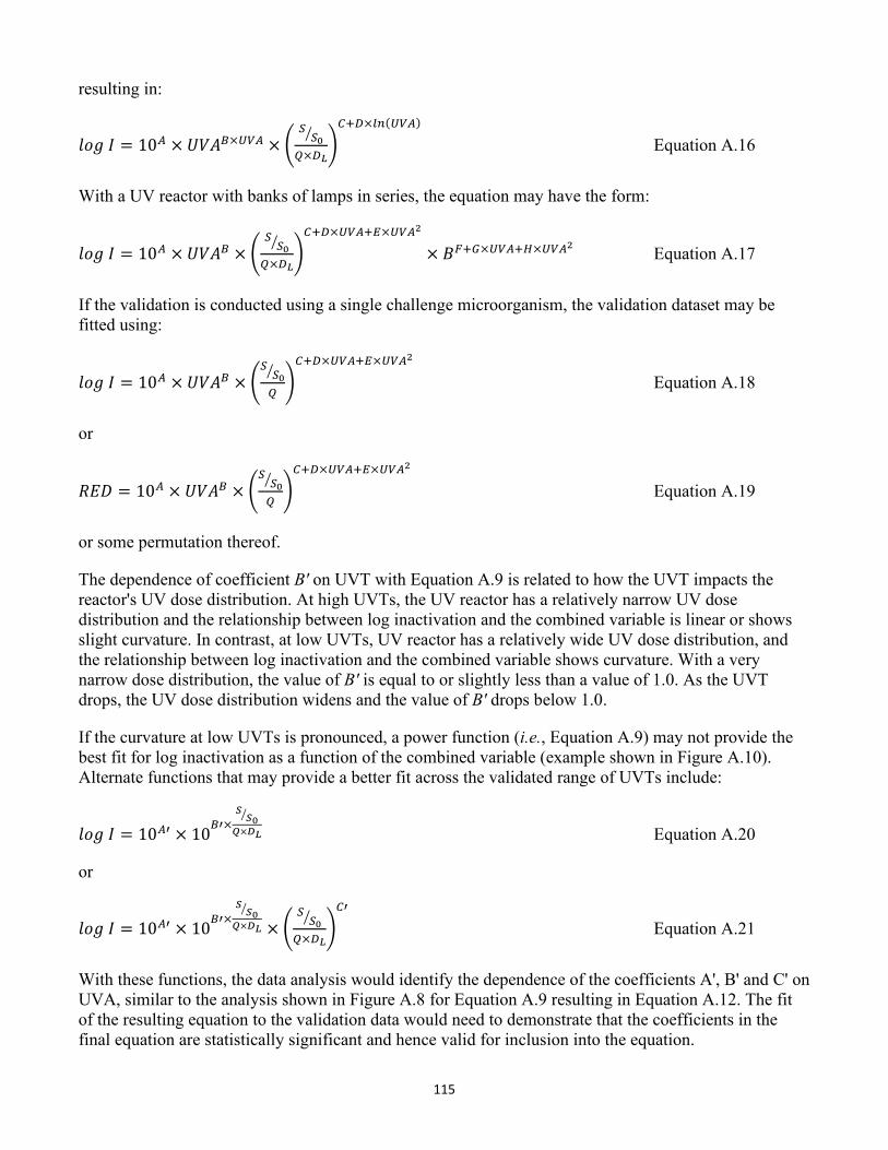
115

resulting in:


𝑄𝑄×𝑅𝑅𝐿𝐿�𝐶𝐶+𝑅𝑅×𝑃𝑃𝑛𝑛(𝑈𝑈𝑈𝑈𝐴𝐴)

Equation A.16

With a UV reactor with banks of lamps in series, the equation may have the form:



× 𝐵𝐵𝐹𝐹+𝐺𝐺×𝑈𝑈𝑈𝑈𝐴𝐴+𝐻𝐻×𝑈𝑈𝑈𝑈𝐴𝐴2 Equation A.17

If the validation is conducted using a single challenge microorganism, the validation dataset may be fitted using:


𝑄𝑄�𝐶𝐶+𝑅𝑅×𝑈𝑈𝑈𝑈𝐴𝐴+𝑅𝑅×𝑈𝑈𝑈𝑈𝐴𝐴2

Equation A.18

or

𝑅𝑅𝑅𝑅𝐷𝐷 = 10𝐴𝐴 × 𝑈𝑈𝑉𝑉𝐴𝐴𝐵𝐵 × �𝑆𝑆𝑆𝑆0�

𝑄𝑄�𝐶𝐶+𝑅𝑅×𝑈𝑈𝑈𝑈𝐴𝐴+𝑅𝑅×𝑈𝑈𝑈𝑈𝐴𝐴2

Equation A.19

or some permutation thereof.

The dependence of coefficient B' on UVT with Equation A.9 is related to how the UVT impacts the reactor's UV dose distribution. At high UVTs, the UV reactor has a relatively narrow UV dose distribution and the relationship between log inactivation and the combined variable is linear or shows slight curvature. In contrast, at low UVTs, UV reactor has a relatively wide UV dose distribution, and the relationship between log inactivation and the combined variable shows curvature. With a very narrow dose distribution, the value of B' is equal to or slightly less than a value of 1.0. As the UVT drops, the UV dose distribution widens and the value of B' drops below 1.0.

If the curvature at low UVTs is pronounced, a power function (i.e., Equation A.9) may not provide the best fit for log inactivation as a function of the combined variable (example shown in Figure A.10). Alternate functions that may provide a better fit across the validated range of UVTs include:

𝑉𝑉𝐷𝐷𝑙𝑙 𝐼𝐼 = 10𝐴𝐴′ × 10𝐵𝐵′×𝑀𝑀𝑀𝑀0�

𝑄𝑄×𝐷𝐷𝐿𝐿

or

Equation A.20

𝑉𝑉𝐷𝐷𝑙𝑙 𝐼𝐼 = 10𝐴𝐴′ × 10𝐵𝐵′×𝑀𝑀𝑀𝑀0�

𝑄𝑄×𝐷𝐷𝐿𝐿 × �𝑆𝑆𝑆𝑆0�

𝑄𝑄×𝑅𝑅𝐿𝐿�𝐶𝐶′

Equation A.21

With these functions, the data analysis would identify the dependence of the coefficients A', B' and C' on UVA, similar to the analysis shown in Figure A.8 for Equation A.9 resulting in Equation A.12. The fit of the resulting equation to the validation data would need to demonstrate that the coefficients in the final equation are statistically significant and hence valid for inclusion into the equation.

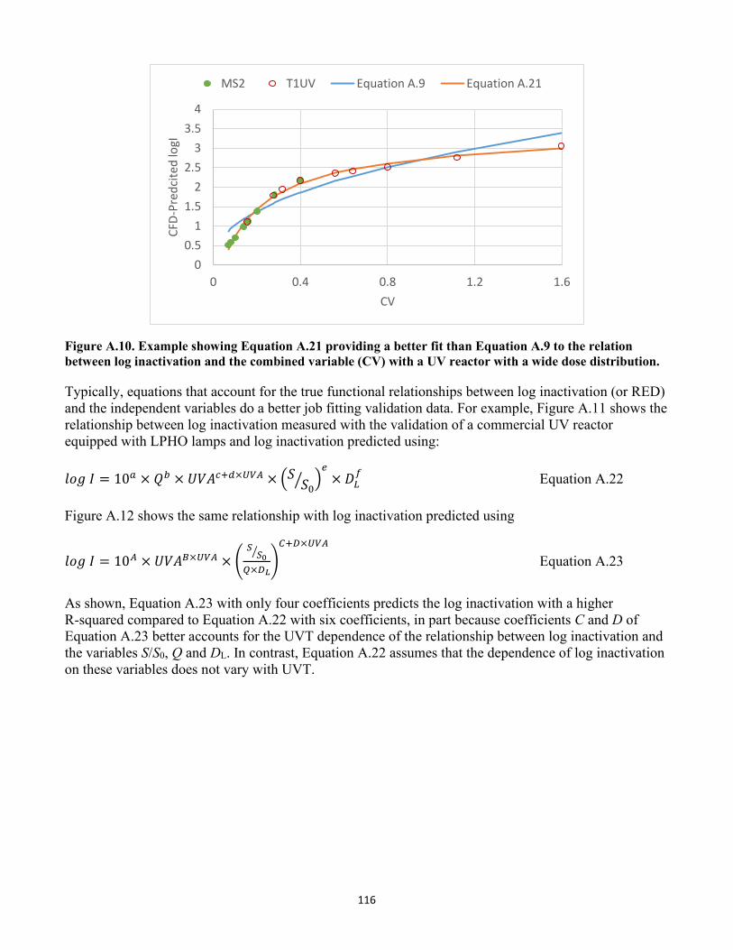
116

00.5

11.5

22.5

33.5

4

0 0.4 0.8 1.2 1.6

CFD-

Pred

cite

d lo

gI

CV

MS2 T1UV Equation A.9 Equation A.21

Figure A.10. Example showing Equation A.21 providing a better fit than Equation A.9 to the relation between log inactivation and the combined variable (CV) with a UV reactor with a wide dose distribution.

Typically, equations that account for the true functional relationships between log inactivation (or RED) and the independent variables do a better job fitting validation data. For example, Figure A.11 shows the relationship between log inactivation measured with the validation of a commercial UV reactor equipped with LPHO lamps and log inactivation predicted using:

𝑉𝑉𝐷𝐷𝑙𝑙 𝐼𝐼 = 10𝑎𝑎 × 𝑄𝑄𝑏𝑏 × 𝑈𝑈𝑉𝑉𝐴𝐴𝑐𝑐+𝑑𝑑×𝑈𝑈𝑈𝑈𝐴𝐴 × �𝑆𝑆 𝑆𝑆0� �𝑒𝑒

× 𝐷𝐷𝐿𝐿𝑓𝑓 Equation A.22

Figure A.12 shows the same relationship with log inactivation predicted using



Equation A.23

As shown, Equation A.23 with only four coefficients predicts the log inactivation with a higher R-squared compared to Equation A.22 with six coefficients, in part because coefficients C and D of Equation A.23 better accounts for the UVT dependence of the relationship between log inactivation and the variables S/S0, Q and DL. In contrast, Equation A.22 assumes that the dependence of log inactivation on these variables does not vary with UVT.

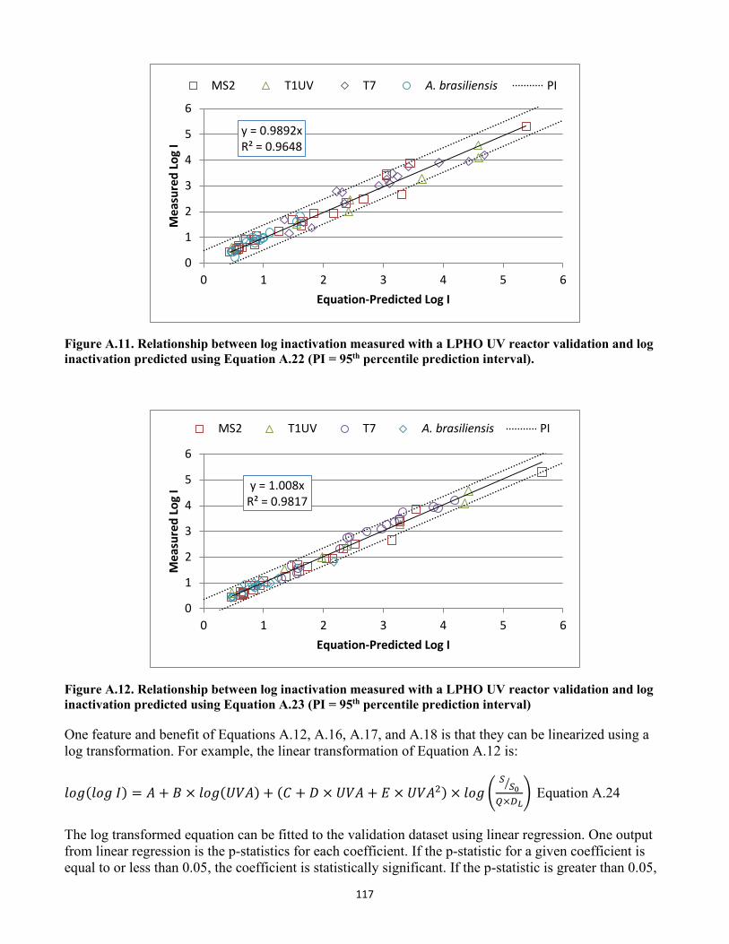
117

y = 0.9892xR² = 0.9648

0

1

2

3

4

5

6

0 1 2 3 4 5 6

Mea

sure

d Lo

g I

Equation-Predicted Log I

MS2 T1UV T7 A. brasiliensis PI

Figure A.11. Relationship between log inactivation measured with a LPHO UV reactor validation and log inactivation predicted using Equation A.22 (PI = 95th percentile prediction interval).

y = 1.008xR² = 0.9817

0

1

2

3

4

5

6

0 1 2 3 4 5 6

Mea

sure

d Lo

g I



Figure A.12. Relationship between log inactivation measured with a LPHO UV reactor validation and log inactivation predicted using Equation A.23 (PI = 95th percentile prediction interval)

One feature and benefit of Equations A.12, A.16, A.17, and A.18 is that they can be linearized using a log transformation. For example, the linear transformation of Equation A.12 is:

𝑉𝑉𝐷𝐷𝑙𝑙(𝑉𝑉𝐷𝐷𝑙𝑙 𝐼𝐼) = 𝐴𝐴 + 𝐵𝐵 × 𝑉𝑉𝐷𝐷𝑙𝑙(𝑈𝑈𝑉𝑉𝐴𝐴) + (𝐴𝐴 + 𝐷𝐷 × 𝑈𝑈𝑉𝑉𝐴𝐴 + 𝑅𝑅 × 𝑈𝑈𝑉𝑉𝐴𝐴2) × 𝑉𝑉𝐷𝐷𝑙𝑙 �𝑆𝑆𝑆𝑆0�

𝑄𝑄×𝑅𝑅𝐿𝐿� Equation A.24

The log transformed equation can be fitted to the validation dataset using linear regression. One output from linear regression is the p-statistics for each coefficient. If the p-statistic for a given coefficient is equal to or less than 0.05, the coefficient is statistically significant. If the p-statistic is greater than 0.05,

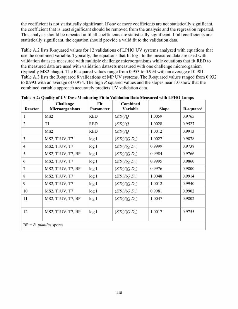
118

the coefficient is not statistically significant. If one or more coefficients are not statistically significant, the coefficient that is least significant should be removed from the analysis and the regression repeated. This analysis should be repeated until all coefficients are statistically significant. If all coefficients are statistically significant, the equation should provide a valid fit to the validation data.

Table A.2 lists R-squared values for 12 validations of LPHO UV systems analyzed with equations that use the combined variable. Typically, the equations that fit log I to the measured data are used with validation datasets measured with multiple challenge microorganisms while equations that fit RED to the measured data are used with validation datasets measured with one challenge microorganism (typically MS2 phage). The R-squared values range from 0.953 to 0.994 with an average of 0.981. Table A.3 lists the R-squared 8 validations of MP UV systems. The R-squared values ranged from 0.932 to 0.993 with an average of 0.974. The high R squared values and the slopes near 1.0 show that the combined variable approach accurately predicts UV validation data.

Table A.2: Quality of UV Dose Monitoring Fit to Validation Data Measured with LPHO Lamps

Reactor Challenge

Microorganisms Fit

Parameter Combined Variable Slope R-squared

1 MS2 RED (S/S0)/Q 1.0059 0.9765

2 T1 RED (S/S0)/Q 1.0028 0.9527

MS2 RED (S/S0)/Q 1.0012 0.9913

3 MS2, T1UV, T7 log I (S/S0)/(Q DL) 1.0027 0.9878


5 MS2, T1UV, T7, BP log I (S/S0)/(Q DL) 0.9984 0.9766








BP = B. pumilus spores

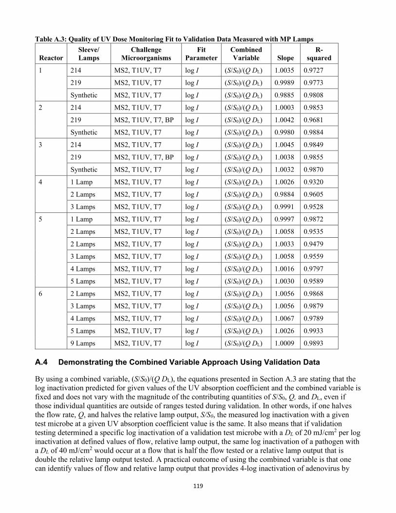
119

Table A.3: Quality of UV Dose Monitoring Fit to Validation Data Measured with MP Lamps

Reactor Sleeve/ Lamps

Challenge Microorganisms

Fit Parameter

Combined Variable Slope

R-squared

1 214 MS2, T1UV, T7 log I (S/S0)/(Q DL) 1.0035 0.9727


Synthetic MS2, T1UV, T7 log I (S/S0)/(Q DL) 0.9885 0.9808







4 1 Lamp MS2, T1UV, T7 log I (S/S0)/(Q DL) 1.0026 0.9320

2 Lamps MS2, T1UV, T7 log I (S/S0)/(Q DL) 0.9884 0.9605


5 1 Lamp MS2, T1UV, T7 log I (S/S0)/(Q DL) 0.9997 0.9872






6 2 Lamps MS2, T1UV, T7 log I (S/S0)/(Q DL) 1.0056 0.9868





A.4 Demonstrating the Combined Variable Approach Using Validation Data

By using a combined variable, (S/S0)/(Q DL), the equations presented in Section A.3 are stating that the log inactivation predicted for given values of the UV absorption coefficient and the combined variable is fixed and does not vary with the magnitude of the contributing quantities of S/S0, Q, and DL, even if those individual quantities are outside of ranges tested during validation. In other words, if one halves the flow rate, Q, and halves the relative lamp output, S/S0, the measured log inactivation with a given test microbe at a given UV absorption coefficient value is the same. It also means that if validation testing determined a specific log inactivation of a validation test microbe with a DL of 20 mJ/cm2 per log inactivation at defined values of flow, relative lamp output, the same log inactivation of a pathogen with a DL of 40 mJ/cm2 would occur at a flow that is half the flow tested or a relative lamp output that is double the relative lamp output tested. A practical outcome of using the combined variable is that one can identify values of flow and relative lamp output that provides 4-log inactivation of adenovirus by

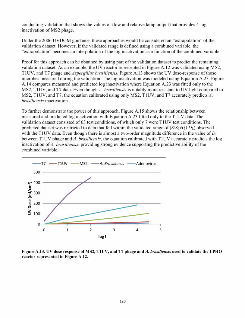
120

conducting validation that shows the values of flow and relative lamp output that provides 4-log inactivation of MS2 phage.

Under the 2006 UVDGM guidance, these approaches would be considered an “extrapolation” of the validation dataset. However, if the validated range is defined using a combined variable, the “extrapolation” becomes an interpolation of the log inactivation as a function of the combined variable.

Proof for this approach can be obtained by using part of the validation dataset to predict the remaining validation dataset. As an example, the UV reactor represented in Figure A.12 was validated using MS2, T1UV, and T7 phage and Aspergillus brasiliensis. Figure A.13 shows the UV dose-response of those microbes measured during the validation. The log inactivation was modeled using Equation A.23. Figure A.14 compares measured and predicted log inactivation where Equation A.23 was fitted only to the MS2, T1UV, and T7 data. Even though A. brasiliensis is notably more resistant to UV light compared to MS2, T1UV, and T7, the equation calibrated using only MS2, T1UV, and T7 accurately predicts A. brasiliensis inactivation.

To further demonstrate the power of this approach, Figure A.15 shows the relationship between measured and predicted log inactivation with Equation A.23 fitted only to the T1UV data. The validation dataset consisted of 63 test conditions, of which only 7 were T1UV test conditions. The predicted dataset was restricted to data that fell within the validated range of (S/S0)/(Q DL) observed with the T1UV data. Even though there is almost a two-order magnitude difference in the value of DL between T1UV phage and A. brasiliensis, the equation calibrated with T1UV accurately predicts the log inactivation of A. brasiliensis, providing strong evidence supporting the predictive ability of the combined variable.

0

100

200

300

400

500

0 1 2 3 4 5

UV

Dose

(mJ/

cm2 )

log I

T7 T1UV MS2 A. Brasiliensis Adenovirus

Figure A.13. UV dose response of MS2, T1UV, and T7 phage and A. brasiliensis used to validate the LPHO reactor represented in Figure A.12.

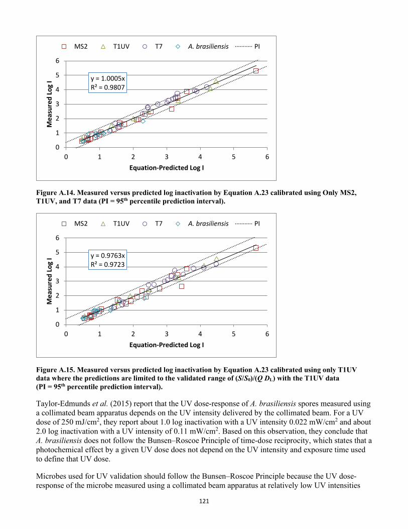
121

y = 1.0005xR² = 0.9807

0

1

2

3

4

5

6

0 1 2 3 4 5 6

Mea

sure

d Lo

g I



Figure A.14. Measured versus predicted log inactivation by Equation A.23 calibrated using Only MS2, T1UV, and T7 data (PI = 95th percentile prediction interval).

y = 0.9763xR² = 0.9723

0

1

2

3

4

5

6

0 1 2 3 4 5 6

Mea

sure

d Lo

g I



Figure A.15. Measured versus predicted log inactivation by Equation A.23 calibrated using only T1UV data where the predictions are limited to the validated range of (S/S0)/(Q DL) with the T1UV data (PI = 95th percentile prediction interval).

Taylor-Edmunds et al. (2015) report that the UV dose-response of A. brasiliensis spores measured using a collimated beam apparatus depends on the UV intensity delivered by the collimated beam. For a UV dose of 250 mJ/cm2, they report about 1.0 log inactivation with a UV intensity 0.022 mW/cm2 and about 2.0 log inactivation with a UV intensity of 0.11 mW/cm2. Based on this observation, they conclude that A. brasiliensis does not follow the Bunsen–Roscoe Principle of time-dose reciprocity, which states that a photochemical effect by a given UV dose does not depend on the UV intensity and exposure time used to define that UV dose.

Microbes used for UV validation should follow the Bunsen–Roscoe Principle because the UV dose-response of the microbe measured using a collimated beam apparatus at relatively low UV intensities

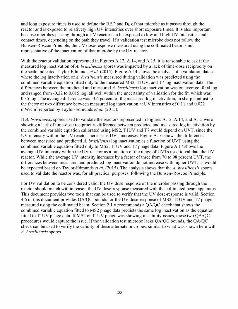
122

and long exposure times is used to define the RED and DL of that microbe as it passes through the reactor and is exposed to relatively high UV intensities over short exposure times. It is also important because microbes passing through a UV reactor can be exposed to low and high UV intensities and contact times, depending on the path they travel. If a validation test microbe does not follow the Bunsen–Roscoe Principle, the UV dose-response measured using the collimated beam is not representative of the inactivation of that microbe by the UV reactor.

With the reactor validation represented in Figures A.12, A.14, and A.15, it is reasonable to ask if the measured log inactivation of A. brasiliensis spores was impacted by a lack of time-dose reciprocity on the scale indicated Taylor-Edmunds et al. (2015). Figure A.14 shows the analysis of a validation dataset where the log inactivation of A. brasiliensis measured during validation was predicted using the combined variable equation fitted only to the measured MS2, T1UV, and T7 log inactivation data. The differences between the predicted and measured A. brasiliensis log inactivation was on average -0.04 log and ranged from -0.22 to 0.015 log, all well within the uncertainty of validation for the fit, which was 0.35 log. The average difference was -3.6 percent of the measured log inactivation, in sharp contrast to the factor of two difference between measured log inactivation at UV intensities of 0.11 and 0.022 mW/cm2 reported by Taylor-Edmunds et al. (2015).

If A. brasiliensis spores used to validate the reactors represented in Figures A.12, A.14, and A.15 were showing a lack of time-dose reciprocity, difference between predicted and measured log inactivation by the combined variable equation calibrated using MS2, T1UV and T7 would depend on UVT, since the UV intensity within the UV reactor increase as UVT increases. Figure A.16 shows the differences between measured and predicted A. brasiliensis log inactivation as a function of UVT using the combined variable equation fitted only to MS2, T1UV and T7 phage data. Figure A.17 shows the average UV intensity within the UV reactor as a function of the range of UVTs used to validate the UV reactor. While the average UV intensity increases by a factor of three from 70 to 98 percent UVT, the differences between measured and predicted log inactivation do not increase with higher UVT, as would be expected based on Taylor-Edmunds et al. (2015). The analysis shows that the A. brasiliensis spores used to validate the reactor was, for all practical purposes, following the Bunsen–Roscoe Principle.

For UV validation to be considered valid, the UV dose response of the microbe passing through the reactor should match within reason the UV dose-response measured with the collimated beam apparatus. This document provides two tools that can be used to verify that the UV dose-response is valid. Section 4.6 of this document provides QA/QC bounds for the UV dose-response of MS2, T1UV and T7 phage measured using the collimated beam. Section 2.1.6 recommends a QA/QC check that shows the combined variable equation fitted to MS2 phage data predicts the same log inactivation as the equation fitted to T1UV phage data. If MS2 or T1UV phage was showing instability issues, these two QA/QC procedures would capture the issue. If the validation test microbe lacks QA/QC bounds, the QA/QC check can be used to verify the validity of these alternate microbes, similar to what was shown here with A. brasiliensis spores.

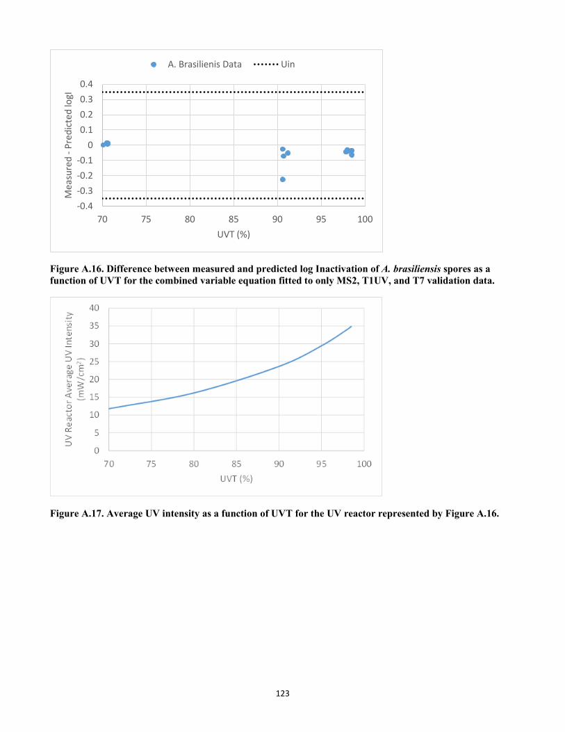
123

-0.4-0.3-0.2-0.1

00.10.20.30.4

70 75 80 85 90 95 100

Mea

sure

d -P

redi

cted

logI

UVT (%)

A. Brasilienis Data Uin

Figure A.16. Difference between measured and predicted log Inactivation of A. brasiliensis spores as a function of UVT for the combined variable equation fitted to only MS2, T1UV, and T7 validation data.

Figure A.17. Average UV intensity as a function of UVT for the UV reactor represented by Figure A.16.

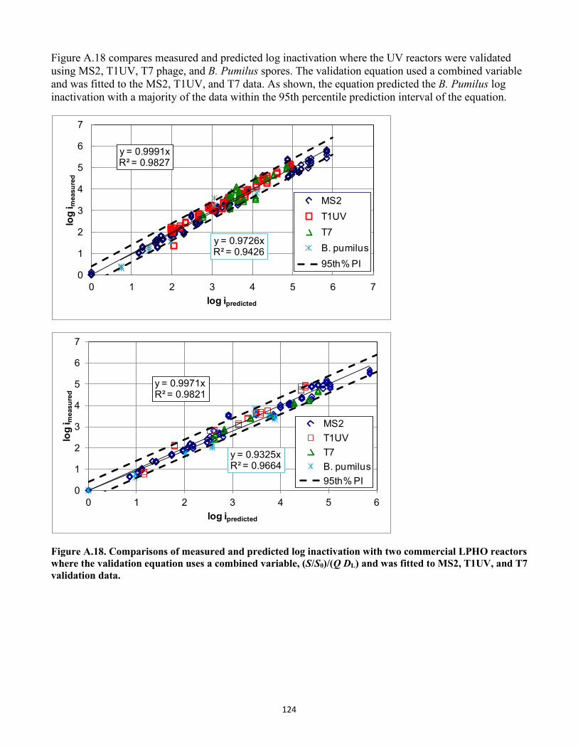
124

Figure A.18 compares measured and predicted log inactivation where the UV reactors were validated using MS2, T1UV, T7 phage, and B. Pumilus spores. The validation equation used a combined variable and was fitted to the MS2, T1UV, and T7 data. As shown, the equation predicted the B. Pumilus log inactivation with a majority of the data within the 95th percentile prediction interval of the equation.

y = 0.9991xR² = 0.9827

y = 0.9726xR² = 0.9426

0

1

2

3

4

5

6

7

0 1 2 3 4 5 6 7

log

i mea

sure

d

log ipredicted

MS2T1UVT7B. pumilus95th% PI

y = 0.9971xR² = 0.9821

y = 0.9325xR² = 0.9664

0

1

2

3

4

5

6

7

0 1 2 3 4 5 6

log

i mea

sure

d

log ipredicted

MS2T1UVT7B. pumilus95th% PI

Figure A.18. Comparisons of measured and predicted log inactivation with two commercial LPHO reactors where the validation equation uses a combined variable, (S/S0)/(Q DL) and was fitted to MS2, T1UV, and T7 validation data.

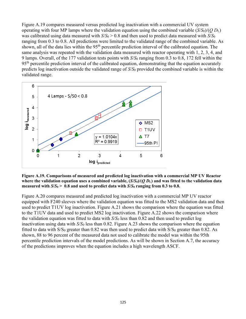
125

Figure A.19 compares measured versus predicted log inactivation with a commercial UV system operating with four MP lamps where the validation equation using the combined variable (S/S0)/(Q DL) was calibrated using data measured with S/S0 > 0.8 and then used to predict data measured with S/S0 ranging from 0.3 to 0.8. All predictions were limited to the validated range of the combined variable. As shown, all of the data lies within the 95th percentile prediction interval of the calibrated equation. The same analysis was repeated with the validation data measured with reactor operating with 1, 2, 3, 4, and 9 lamps. Overall, of the 177 validation tests points with S/S0 ranging from 0.3 to 0.8, 172 fell within the 95th percentile prediction interval of the calibrated equation, demonstrating that the equation accurately predicts log inactivation outside the validated range of S/S0 provided the combined variable is within the validated range.

Figure A.19. Comparisons of measured and predicted log inactivation with a commercial MP UV Reactor where the validation equation uses a combined variable, (S/S0)/(Q DL) and was fitted to the validation data measured with S/S0 > 0.8 and used to predict data with S/S0 ranging from 0.3 to 0.8.

Figure A.20 compares measured and predicted log inactivation with a commercial MP UV reactor equipped with F240 sleeves where the validation equation was fitted to the MS2 validation data and then used to predict T1UV log inactivation. Figure A.21 shows the comparison where the equation was fitted to the T1UV data and used to predict MS2 log inactivation. Figure A.22 shows the comparison where the validation equation was fitted to data with S/S0 less than 0.82 and then used to predict log inactivation using data with S/S0 less than 0.82. Figure A.23 shows the comparison where the equation fitted to data with S/S0 greater than 0.82 was then used to predict data with S/S0 greater than 0.82. As shown, 88 to 96 percent of the measured data not used to calibrate the model was within the 95th percentile prediction intervals of the model predictions. As will be shown in Section A.7, the accuracy of the predictions improves when the equation includes a high wavelength ASCF.

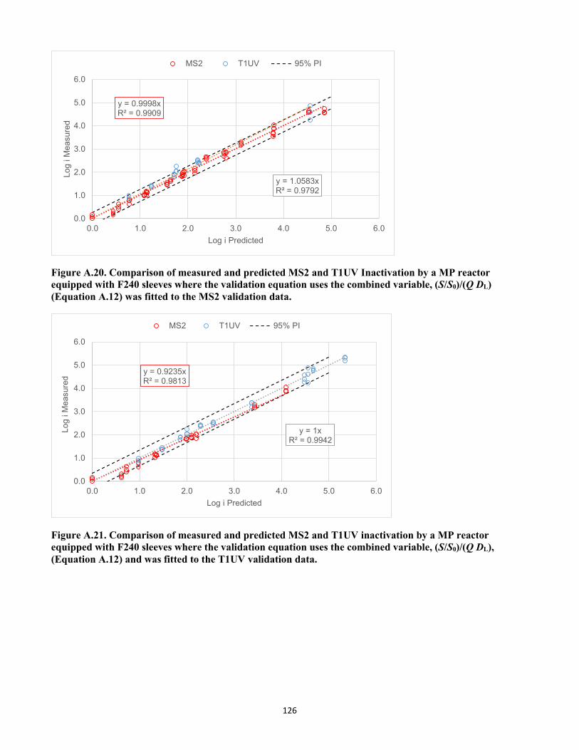
126

y = 0.9998xR² = 0.9909

y = 1.0583xR² = 0.9792

0.0

1.0

2.0

3.0

4.0

5.0

6.0

0.0 1.0 2.0 3.0 4.0 5.0 6.0

Log

i Mea

sure

d

Log i Predicted

MS2 T1UV 95% PI

Figure A.20. Comparison of measured and predicted MS2 and T1UV Inactivation by a MP reactor equipped with F240 sleeves where the validation equation uses the combined variable, (S/S0)/(Q DL) (Equation A.12) was fitted to the MS2 validation data.

y = 0.9235xR² = 0.9813

y = 1xR² = 0.9942

0.0

1.0

2.0

3.0

4.0

5.0

6.0

0.0 1.0 2.0 3.0 4.0 5.0 6.0

Log

i Mea

sure

d

Log i Predicted

MS2 T1UV 95% PI

Figure A.21. Comparison of measured and predicted MS2 and T1UV inactivation by a MP reactor equipped with F240 sleeves where the validation equation uses the combined variable, (S/S0)/(Q DL), (Equation A.12) and was fitted to the T1UV validation data.

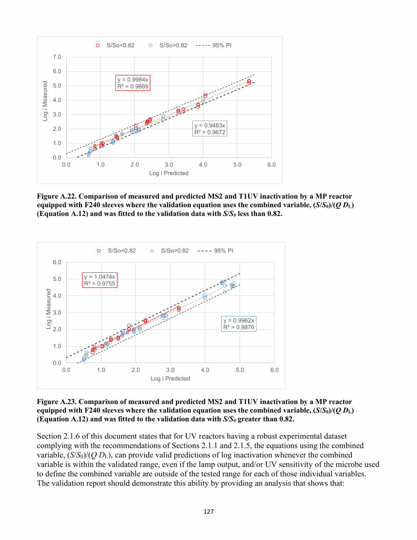
127

y = 0.9984xR² = 0.9889

y = 0.9483xR² = 0.9672

0.0

1.0

2.0

3.0

4.0

5.0

6.0

7.0

0.0 1.0 2.0 3.0 4.0 5.0 6.0

Log

i Mea

sure

d

Log i Predicted

S/So<0.82 S/So>0.82 95% PI

Figure A.22. Comparison of measured and predicted MS2 and T1UV inactivation by a MP reactor equipped with F240 sleeves where the validation equation uses the combined variable, (S/S0)/(Q DL) (Equation A.12) and was fitted to the validation data with S/S0 less than 0.82.

y = 1.0474xR² = 0.9755

y = 0.9962xR² = 0.9876

0.0

1.0

2.0

3.0

4.0

5.0

6.0

0.0 1.0 2.0 3.0 4.0 5.0 6.0

Log

i Mea

sure

d

Log i Predicted

S/So<0.82 S/So>0.82 95% PI

Figure A.23. Comparison of measured and predicted MS2 and T1UV inactivation by a MP reactor equipped with F240 sleeves where the validation equation uses the combined variable, (S/S0)/(Q DL) (Equation A.12) and was fitted to the validation data with S/S0 greater than 0.82.

Section 2.1.6 of this document states that for UV reactors having a robust experimental dataset complying with the recommendations of Sections 2.1.1 and 2.1.5, the equations using the combined variable, (S/S0)/(Q DL), can provide valid predictions of log inactivation whenever the combined variable is within the validated range, even if the lamp output, and/or UV sensitivity of the microbe used to define the combined variable are outside of the tested range for each of those individual variables. The validation report should demonstrate this ability by providing an analysis that shows that:

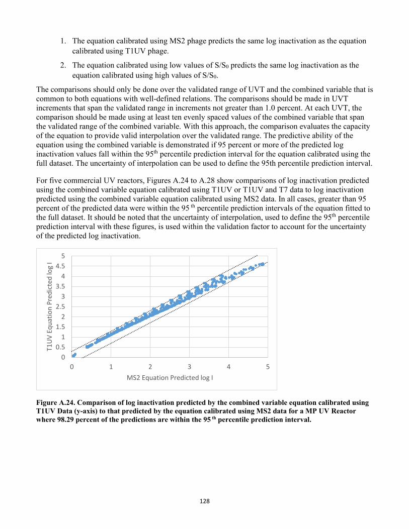
128

1. The equation calibrated using MS2 phage predicts the same log inactivation as the equation calibrated using T1UV phage.

2. The equation calibrated using low values of S/S0 predicts the same log inactivation as the equation calibrated using high values of S/S0.

The comparisons should only be done over the validated range of UVT and the combined variable that is common to both equations with well-defined relations. The comparisons should be made in UVT increments that span the validated range in increments not greater than 1.0 percent. At each UVT, the comparison should be made using at least ten evenly spaced values of the combined variable that span the validated range of the combined variable. With this approach, the comparison evaluates the capacity of the equation to provide valid interpolation over the validated range. The predictive ability of the equation using the combined variable is demonstrated if 95 percent or more of the predicted log inactivation values fall within the 95th percentile prediction interval for the equation calibrated using the full dataset. The uncertainty of interpolation can be used to define the 95th percentile prediction interval.

For five commercial UV reactors, Figures A.24 to A.28 show comparisons of log inactivation predicted using the combined variable equation calibrated using T1UV or T1UV and T7 data to log inactivation predicted using the combined variable equation calibrated using MS2 data. In all cases, greater than 95 percent of the predicted data were within the 95 th percentile prediction intervals of the equation fitted to the full dataset. It should be noted that the uncertainty of interpolation, used to define the 95th percentile prediction interval with these figures, is used within the validation factor to account for the uncertainty of the predicted log inactivation.

00.5

11.5

22.5

33.5

44.5

5

0 1 2 3 4 5

T1U

V Eq

uatio

n Pr

edic

ted

log

I

MS2 Equation Predicted log I

Figure A.24. Comparison of log inactivation predicted by the combined variable equation calibrated using T1UV Data (y-axis) to that predicted by the equation calibrated using MS2 data for a MP UV Reactor where 98.29 percent of the predictions are within the 95 th percentile prediction interval.

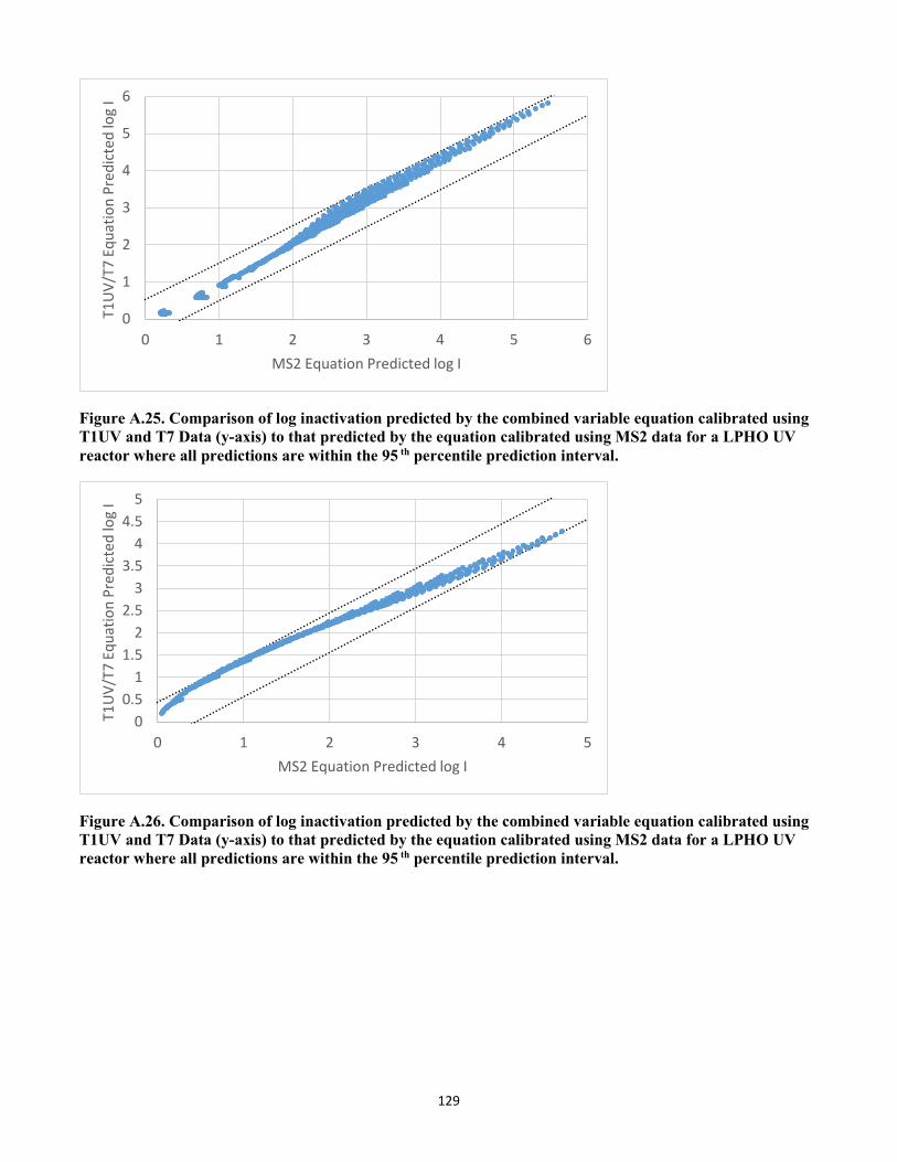
129

0

1

2

3

4

5

6

0 1 2 3 4 5 6

T1U

V/T7

Equ

atio

n Pr

edic

ted

log

I


Figure A.25. Comparison of log inactivation predicted by the combined variable equation calibrated using T1UV and T7 Data (y-axis) to that predicted by the equation calibrated using MS2 data for a LPHO UV reactor where all predictions are within the 95 th percentile prediction interval.

00.5

11.5

22.5

33.5

44.5

5

0 1 2 3 4 5

T1U

V/T7

Equ

atio

n Pr

edic

ted

log

I


Figure A.26. Comparison of log inactivation predicted by the combined variable equation calibrated using T1UV and T7 Data (y-axis) to that predicted by the equation calibrated using MS2 data for a LPHO UV reactor where all predictions are within the 95 th percentile prediction interval.

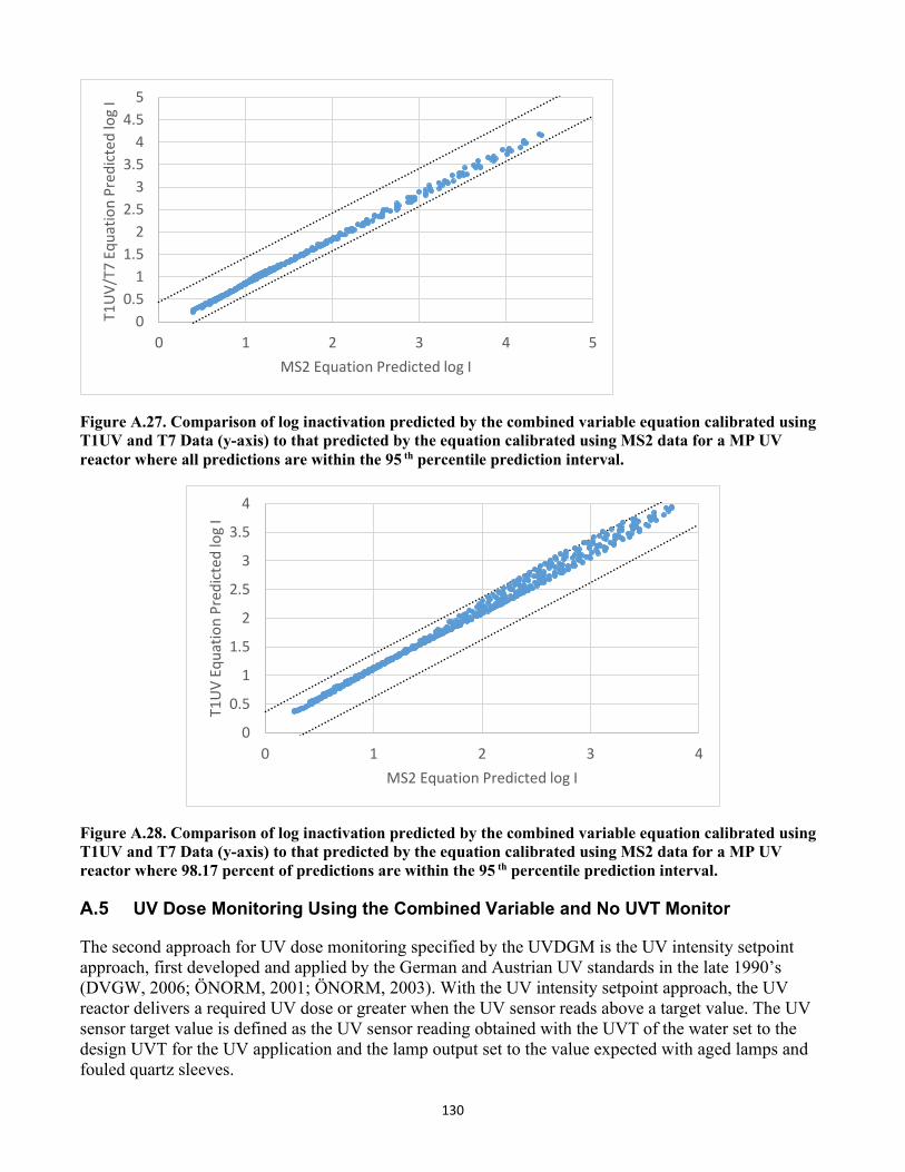
130

00.5

11.5

22.5

33.5

44.5

5

0 1 2 3 4 5

T1U

V/T7

Equ

atio

n Pr

edic

ted

log

I


Figure A.27. Comparison of log inactivation predicted by the combined variable equation calibrated using T1UV and T7 Data (y-axis) to that predicted by the equation calibrated using MS2 data for a MP UV reactor where all predictions are within the 95 th percentile prediction interval.

0

0.5

1

1.5

2

2.5

3

3.5

4

0 1 2 3 4

T1U

V Eq

uatio

n Pr

edic

ted

log

I


Figure A.28. Comparison of log inactivation predicted by the combined variable equation calibrated using T1UV and T7 Data (y-axis) to that predicted by the equation calibrated using MS2 data for a MP UV reactor where 98.17 percent of predictions are within the 95 th percentile prediction interval.

A.5 UV Dose Monitoring Using the Combined Variable and No UVT Monitor

The second approach for UV dose monitoring specified by the UVDGM is the UV intensity setpoint approach, first developed and applied by the German and Austrian UV standards in the late 1990’s (DVGW, 2006; ÖNORM, 2001; ÖNORM, 2003). With the UV intensity setpoint approach, the UV reactor delivers a required UV dose or greater when the UV sensor reads above a target value. The UV sensor target value is defined as the UV sensor reading obtained with the UVT of the water set to the design UVT for the UV application and the lamp output set to the value expected with aged lamps and fouled quartz sleeves.

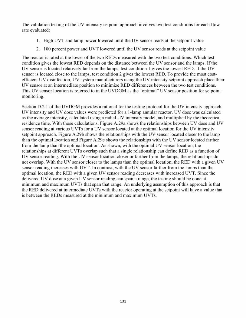
131

The validation testing of the UV intensity setpoint approach involves two test conditions for each flow rate evaluated:

1. High UVT and lamp power lowered until the UV sensor reads at the setpoint value

2. 100 percent power and UVT lowered until the UV sensor reads at the setpoint value

The reactor is rated at the lower of the two REDs measured with the two test conditions. Which test condition gives the lowest RED depends on the distance between the UV sensor and the lamps. If the UV sensor is located relatively far from the lamps, test condition 1 gives the lowest RED. If the UV sensor is located close to the lamps, test condition 2 gives the lowest RED. To provide the most cost-efficient UV disinfection, UV system manufacturers using the UV intensity setpoint approach place their UV sensor at an intermediate position to minimize RED differences between the two test conditions. This UV sensor location is referred to in the UVDGM as the “optimal” UV sensor position for setpoint monitoring.

Section D.2.1 of the UVDGM provides a rational for the testing protocol for the UV intensity approach. UV intensity and UV dose values were predicted for a 1-lamp annular reactor. UV dose was calculated as the average intensity, calculated using a radial UV intensity model, and multiplied by the theoretical residence time. With those calculations, Figure A.29a shows the relationships between UV dose and UV sensor reading at various UVTs for a UV sensor located at the optimal location for the UV intensity setpoint approach. Figure A.29b shows the relationships with the UV sensor located closer to the lamp than the optimal location and Figure A.29c shows the relationships with the UV sensor located farther from the lamp than the optimal location. As shown, with the optimal UV sensor location, the relationships at different UVTs overlap such that a single relationship can define RED as a function of UV sensor reading. With the UV sensor location closer or farther from the lamps, the relationships do not overlap. With the UV sensor closer to the lamps than the optimal location, the RED with a given UV sensor reading increases with UVT. In contrast, with the UV sensor farther from the lamps than the optimal location, the RED with a given UV sensor reading decreases with increased UVT. Since the delivered UV dose at a given UV sensor reading can span a range, the testing should be done at minimum and maximum UVTs that span that range. An underlying assumption of this approach is that the RED delivered at intermediate UVTs with the reactor operating at the setpoint will have a value that is between the REDs measured at the minimum and maximum UVTs.

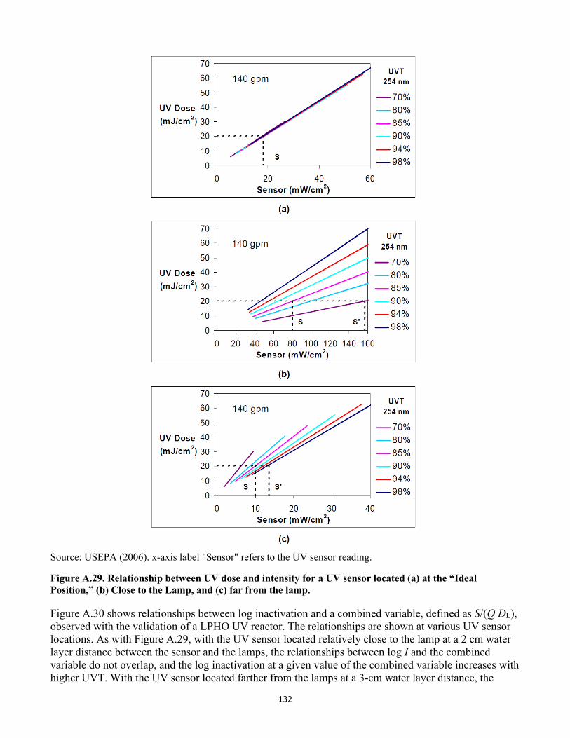
132

Source: USEPA (2006). x-axis label "Sensor" refers to the UV sensor reading.

Figure A.29. Relationship between UV dose and intensity for a UV sensor located (a) at the “Ideal Position,” (b) Close to the Lamp, and (c) far from the lamp.

Figure A.30 shows relationships between log inactivation and a combined variable, defined as S/(Q DL), observed with the validation of a LPHO UV reactor. The relationships are shown at various UV sensor locations. As with Figure A.29, with the UV sensor located relatively close to the lamp at a 2 cm water layer distance between the sensor and the lamps, the relationships between log I and the combined variable do not overlap, and the log inactivation at a given value of the combined variable increases with higher UVT. With the UV sensor located farther from the lamps at a 3-cm water layer distance, the

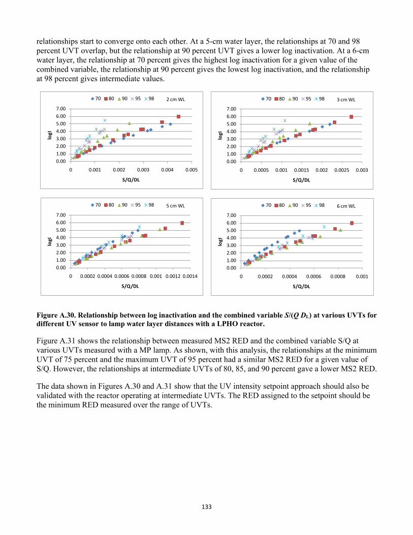
133

relationships start to converge onto each other. At a 5-cm water layer, the relationships at 70 and 98 percent UVT overlap, but the relationship at 90 percent UVT gives a lower log inactivation. At a 6-cm water layer, the relationship at 70 percent gives the highest log inactivation for a given value of the combined variable, the relationship at 90 percent gives the lowest log inactivation, and the relationship at 98 percent gives intermediate values.

0.001.002.003.004.005.006.007.00

0 0.001 0.002 0.003 0.004 0.005

logI

S/Q/DL

70 80 90 95 98 2 cm WL

0.001.002.003.004.005.006.007.00

0 0.0002 0.0004 0.0006 0.0008 0.001 0.0012 0.0014

logI

S/Q/DL

70 80 90 95 98 5 cm WL

0.001.002.003.004.005.006.007.00

0 0.0005 0.001 0.0015 0.002 0.0025 0.003

logI

S/Q/DL

70 80 90 95 98 3 cm WL

0.001.002.003.004.005.006.007.00

0 0.0002 0.0004 0.0006 0.0008 0.001

logI

S/Q/DL

70 80 90 95 98 6 cm WL

Figure A.30. Relationship between log inactivation and the combined variable S/(Q DL) at various UVTs for different UV sensor to lamp water layer distances with a LPHO reactor.

Figure A.31 shows the relationship between measured MS2 RED and the combined variable S/Q at various UVTs measured with a MP lamp. As shown, with this analysis, the relationships at the minimum UVT of 75 percent and the maximum UVT of 95 percent had a similar MS2 RED for a given value of S/Q. However, the relationships at intermediate UVTs of 80, 85, and 90 percent gave a lower MS2 RED.

The data shown in Figures A.30 and A.31 show that the UV intensity setpoint approach should also be validated with the reactor operating at intermediate UVTs. The RED assigned to the setpoint should be the minimum RED measured over the range of UVTs.

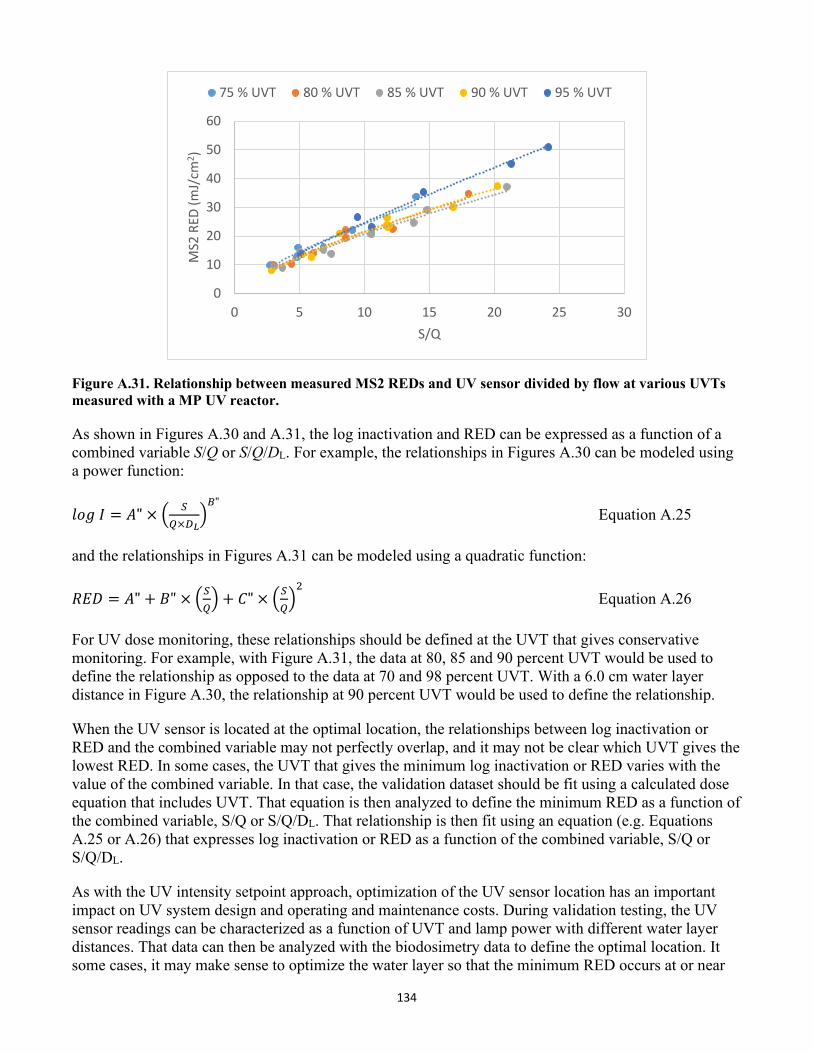
134

0

10

20

30

40

50

60

0 5 10 15 20 25 30

MS2

RED

(mJ/

cm2 )

S/Q

75 % UVT 80 % UVT 85 % UVT 90 % UVT 95 % UVT

Figure A.31. Relationship between measured MS2 REDs and UV sensor divided by flow at various UVTs measured with a MP UV reactor.

As shown in Figures A.30 and A.31, the log inactivation and RED can be expressed as a function of a combined variable S/Q or S/Q/DL. For example, the relationships in Figures A.30 can be modeled using a power function:

𝑉𝑉𝐷𝐷𝑙𝑙 𝐼𝐼 = 𝐴𝐴" × � 𝑆𝑆𝑄𝑄×𝑅𝑅𝐿𝐿

�𝐵𝐵"

Equation A.25

and the relationships in Figures A.31 can be modeled using a quadratic function:

𝑅𝑅𝑅𝑅𝐷𝐷 = 𝐴𝐴" + 𝐵𝐵" × �𝑆𝑆𝑄𝑄� + 𝐴𝐴" × �𝑆𝑆

𝑄𝑄�2 Equation A.26

For UV dose monitoring, these relationships should be defined at the UVT that gives conservative monitoring. For example, with Figure A.31, the data at 80, 85 and 90 percent UVT would be used to define the relationship as opposed to the data at 70 and 98 percent UVT. With a 6.0 cm water layer distance in Figure A.30, the relationship at 90 percent UVT would be used to define the relationship.

When the UV sensor is located at the optimal location, the relationships between log inactivation or RED and the combined variable may not perfectly overlap, and it may not be clear which UVT gives the lowest RED. In some cases, the UVT that gives the minimum log inactivation or RED varies with the value of the combined variable. In that case, the validation dataset should be fit using a calculated dose equation that includes UVT. That equation is then analyzed to define the minimum RED as a function of the combined variable, S/Q or S/Q/DL. That relationship is then fit using an equation (e.g. Equations A.25 or A.26) that expresses log inactivation or RED as a function of the combined variable, S/Q or S/Q/DL.

As with the UV intensity setpoint approach, optimization of the UV sensor location has an important impact on UV system design and operating and maintenance costs. During validation testing, the UV sensor readings can be characterized as a function of UVT and lamp power with different water layer distances. That data can then be analyzed with the biodosimetry data to define the optimal location. It some cases, it may make sense to optimize the water layer so that the minimum RED occurs at or near

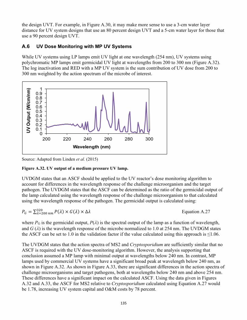
135

the design UVT. For example, in Figure A.30, it may make more sense to use a 3-cm water layer distance for UV system designs that use an 80 percent design UVT and a 5-cm water layer for those that use a 90 percent design UVT.

A.6 UV Dose Monitoring with MP UV Systems

While UV systems using LP lamps emit UV light at one wavelength (254 nm), UV systems using polychromatic MP lamps emit germicidal UV light at wavelengths from 200 to 300 nm (Figure A.32). The log inactivation and RED with a MP UV system is the sum contribution of UV dose from 200 to 300 nm weighted by the action spectrum of the microbe of interest.

00.10.20.30.40.50.60.70.80.9

1

200 220 240 260 280 300

UV O

utpu

t (W

/cm

/nm

)

Wavelength (nm)

Source: Adapted from Linden et al. (2015)

Figure A.32. UV output of a medium pressure UV lamp.

UVDGM states that an ASCF should be applied to the UV reactor’s dose monitoring algorithm to account for differences in the wavelength response of the challenge microorganism and the target pathogen. The UVDGM states that the ASCF can be determined as the ratio of the germicidal output of the lamp calculated using the wavelength response of the challenge microorganism to that calculated using the wavelength response of the pathogen. The germicidal output is calculated using:

𝑃𝑃𝐺𝐺 = ∑ 𝑃𝑃(𝜆𝜆) × 𝐺𝐺(𝜆𝜆) × ∆𝜆𝜆320𝜆𝜆=200 𝑛𝑛𝑛𝑛 Equation A.27

where PG is the germicidal output, P(λ) is the spectral output of the lamp as a function of wavelength, and G (λ) is the wavelength response of the microbe normalized to 1.0 at 254 nm. The UVDGM states the ASCF can be set to 1.0 in the validation factor if the value calculated using this approach is ≤1.06.

The UVDGM states that the action spectra of MS2 and Cryptosporidium are sufficiently similar that no ASCF is required with the UV dose-monitoring algorithm. However, the analysis supporting that conclusion assumed a MP lamp with minimal output at wavelengths below 240 nm. In contrast, MP lamps used by commercial UV systems have a significant broad peak at wavelength below 240 nm, as shown in Figure A.32. As shown in Figure A.33, there are significant differences in the action spectra of challenge microorganisms and target pathogens, both at wavelengths below 240 nm and above 254 nm. These differences have a significant impact on the calculated ASCF. Using the data given in Figures A.32 and A.33, the ASCF for MS2 relative to Cryptosporidium calculated using Equation A.27 would be 1.78, increasing UV system capital and O&M costs by 78 percent.

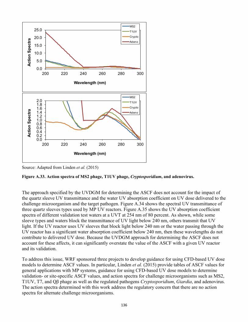
136

0.0

5.0

10.0

15.0

20.0

25.0

200 220 240 260 280 300

Actio

n Sp

ectra

Wavelength (nm)

MS2

T1UV

Crypto

Adeno

0.00.20.40.60.81.01.21.41.61.82.0

200 220 240 260 280 300

Actio

n Sp

ectra

Wavelength (nm)

MS2

T1UV

Crypto

Adeno


Figure A.33. Action spectra of MS2 phage, T1UV phage, Cryptosporidium, and adenovirus.

The approach specified by the UVDGM for determining the ASCF does not account for the impact of the quartz sleeve UV transmittance and the water UV absorption coefficient on UV dose delivered to the challenge microorganism and the target pathogen. Figure A.34 shows the spectral UV transmittance of three quartz sleeves types used by MP UV reactors. Figure A.35 shows the UV absorption coefficient spectra of different validation test waters at a UVT at 254 nm of 80 percent. As shown, while some sleeve types and waters block the transmittance of UV light below 240 nm, others transmit that UV light. If the UV reactor uses UV sleeves that block light below 240 nm or the water passing through the UV reactor has a significant water absorption coefficient below 240 nm, then these wavelengths do not contribute to delivered UV dose. Because the UVDGM approach for determining the ASCF does not account for these affects, it can significantly overstate the value of the ASCF with a given UV reactor and its validation.

To address this issue, WRF sponsored three projects to develop guidance for using CFD-based UV dose models to determine ASCF values. In particular, Linden et al. (2015) provide tables of ASCF values for general applications with MP systems, guidance for using CFD-based UV dose models to determine validation- or site-specific ASCF values, and action spectra for challenge microorganisms such as MS2, T1UV, T7, and Qβ phage as well as the regulated pathogens Cryptosporidium, Giardia, and adenovirus. The action spectra determined with this work address the regulatory concern that there are no action spectra for alternate challenge microorganisms.

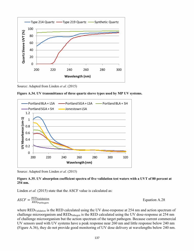
137

0

20

40

60

80

100

200 220 240 260 280 300

Qua

rtz S

leev

e UV

T (%

)

Wavelength (nm)

Type 214 Quartz Type 219 Quartz Synthetic Quartz


Figure A.34. UV transmittance of three quartz sleeve types used by MP UV systems.

0

0.2

0.4

0.6

0.8

1

1.2

200 220 240 260 280 300 320

UV

Abso

rban

ce (c

m-1

)

Wavelength (nm)

Portland BLA + LSA Portland SGA + LSA Portland BLA + SHPortland SGA + SH Jonestown LSA


Figure A.35. UV absorption coefficient spectra of five validation test waters with a UVT of 80 percent at 254 nm.

Linden et al. (2015) state that the ASCF value is calculated as:

𝐴𝐴𝑆𝑆𝐴𝐴𝑉𝑉 = 𝑅𝑅𝑅𝑅𝑅𝑅𝑉𝑉𝑉𝑉𝑉𝑉𝑉𝑉𝑉𝑉𝑉𝑉𝑉𝑉𝑉𝑉𝑉𝑉𝑉𝑉𝑅𝑅𝑅𝑅𝑅𝑅𝑃𝑃𝑉𝑉𝑉𝑉ℎ𝑉𝑉𝑜𝑜𝑜𝑜𝑉𝑉

Equation A.28

where REDValidation is the RED calculated using the UV dose-response at 254 nm and action spectrum of challenge microorganism and REDPathogen is the RED calculated using the UV dose-response at 254 nm of challenge microorganism but the action spectrum of the target pathogen. Because current commercial UV sensors used with UV systems have a peak response near 260 nm and little response below 240 nm (Figure A.36), they do not provide good monitoring of UV dose delivery at wavelengths below 240 nm.

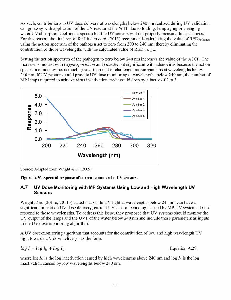
138

As such, contributions to UV dose delivery at wavelengths below 240 nm realized during UV validation can go away with application of the UV reactor at the WTP due to fouling, lamp aging or changing water UV absorption coefficient spectra but the UV sensors will not properly measure those changes. For this reason, the final report for Linden et al. (2015) recommends calculating the value of REDPathogen using the action spectrum of the pathogen set to zero from 200 to 240 nm, thereby eliminating the contribution of those wavelengths with the calculated value of REDPathogen.

Setting the action spectrum of the pathogen to zero below 240 nm increases the value of the ASCF. The increase is modest with Cryptosporidium and Giardia but significant with adenovirus because the action spectrum of adenovirus is much greater than that of challenge microorganisms at wavelengths below 240 nm. If UV reactors could provide UV dose monitoring at wavelengths below 240 nm, the number of MP lamps required to achieve virus inactivation credit could drop by a factor of 2 to 3.

0.01.02.03.04.05.0

200 220 240 260 280 300 320

Res

pons

e

Wavelength (nm)

MS2 4376

Vendor 1

Vendor 2

Vendor 3

Vendor 4

Source: Adapted from Wright et al. (2009)

Figure A.36. Spectral response of current commercial UV sensors.

A.7 UV Dose Monitoring with MP Systems Using Low and High Wavelength UV Sensors

Wright et al. (2011a, 2011b) stated that while UV light at wavelengths below 240 nm can have a significant impact on UV dose delivery, current UV sensor technologies used by MP UV systems do not respond to those wavelengths. To address this issue, they proposed that UV systems should monitor the UV output of the lamps and the UVT of the water below 240 nm and include those parameters as inputs to the UV dose monitoring algorithm.

A UV dose-monitoring algorithm that accounts for the contribution of low and high wavelength UV light towards UV dose delivery has the form:

𝑉𝑉𝐷𝐷𝑙𝑙 𝐼𝐼 = 𝑉𝑉𝐷𝐷𝑙𝑙 𝐼𝐼𝐻𝐻 + 𝑉𝑉𝐷𝐷𝑙𝑙 𝐼𝐼𝐿𝐿 Equation A.29

where log IH is the log inactivation caused by high wavelengths above 240 nm and log IL is the log inactivation caused by low wavelengths below 240 nm.

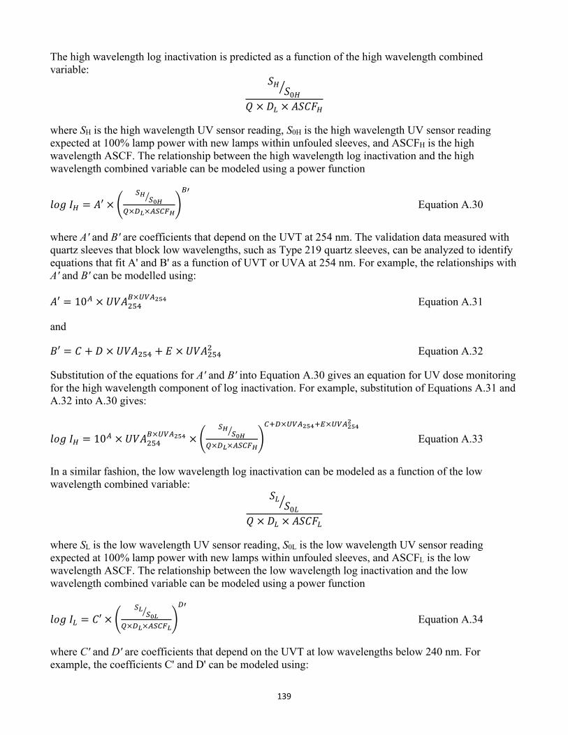
139

The high wavelength log inactivation is predicted as a function of the high wavelength combined variable:



where SH is the high wavelength UV sensor reading, S0H is the high wavelength UV sensor reading expected at 100% lamp power with new lamps within unfouled sleeves, and ASCFH is the high wavelength ASCF. The relationship between the high wavelength log inactivation and the high wavelength combined variable can be modeled using a power function

𝑉𝑉𝐷𝐷𝑙𝑙 𝐼𝐼𝐻𝐻 = 𝐴𝐴′ × �𝑆𝑆𝐻𝐻


𝑄𝑄×𝑅𝑅𝐿𝐿×𝐴𝐴𝑆𝑆𝐶𝐶𝐹𝐹𝐻𝐻�𝐵𝐵′

Equation A.30

where A' and B' are coefficients that depend on the UVT at 254 nm. The validation data measured with quartz sleeves that block low wavelengths, such as Type 219 quartz sleeves, can be analyzed to identify equations that fit A' and B' as a function of UVT or UVA at 254 nm. For example, the relationships with A' and B' can be modelled using:

𝐴𝐴′ = 10𝐴𝐴 × 𝑈𝑈𝑉𝑉𝐴𝐴254𝐵𝐵×𝑈𝑈𝑈𝑈𝐴𝐴254 Equation A.31

and

𝐵𝐵′ = 𝐴𝐴 + 𝐷𝐷 × 𝑈𝑈𝑉𝑉𝐴𝐴254 + 𝑅𝑅 × 𝑈𝑈𝑉𝑉𝐴𝐴2542 Equation A.32

Substitution of the equations for A' and B' into Equation A.30 gives an equation for UV dose monitoring for the high wavelength component of log inactivation. For example, substitution of Equations A.31 and A.32 into A.30 gives:

𝑉𝑉𝐷𝐷𝑙𝑙 𝐼𝐼𝐻𝐻 = 10𝐴𝐴 × 𝑈𝑈𝑉𝑉𝐴𝐴254𝐵𝐵×𝑈𝑈𝑈𝑈𝐴𝐴254 × �



Equation A.33

In a similar fashion, the low wavelength log inactivation can be modeled as a function of the low wavelength combined variable:



where SL is the low wavelength UV sensor reading, S0L is the low wavelength UV sensor reading expected at 100% lamp power with new lamps within unfouled sleeves, and ASCFL is the low wavelength ASCF. The relationship between the low wavelength log inactivation and the low wavelength combined variable can be modeled using a power function

𝑉𝑉𝐷𝐷𝑙𝑙 𝐼𝐼𝐿𝐿 = 𝐴𝐴′ × �𝑆𝑆𝐿𝐿


𝑄𝑄×𝑅𝑅𝐿𝐿×𝐴𝐴𝑆𝑆𝐶𝐶𝐹𝐹𝐿𝐿�𝑅𝑅′

Equation A.34

where C' and D' are coefficients that depend on the UVT at low wavelengths below 240 nm. For example, the coefficients C' and D' can be modeled using:

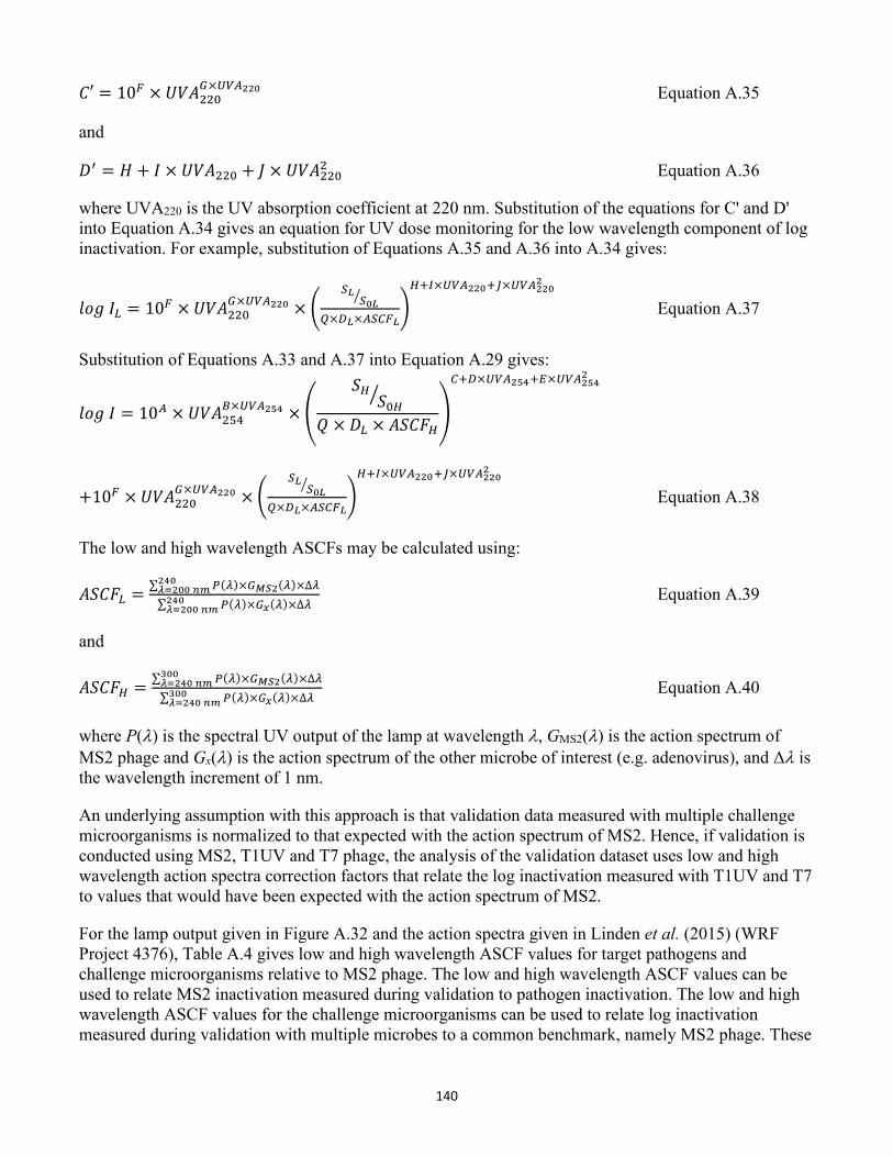
140

𝐴𝐴′ = 10𝐹𝐹 × 𝑈𝑈𝑉𝑉𝐴𝐴220𝐺𝐺×𝑈𝑈𝑈𝑈𝐴𝐴220 Equation A.35

and

𝐷𝐷′ = 𝐻𝐻 + 𝐼𝐼 × 𝑈𝑈𝑉𝑉𝐴𝐴220 + 𝐽𝐽 × 𝑈𝑈𝑉𝑉𝐴𝐴2202 Equation A.36

where UVA220 is the UV absorption coefficient at 220 nm. Substitution of the equations for C' and D' into Equation A.34 gives an equation for UV dose monitoring for the low wavelength component of log inactivation. For example, substitution of Equations A.35 and A.36 into A.34 gives:

𝑉𝑉𝐷𝐷𝑙𝑙 𝐼𝐼𝐿𝐿 = 10𝐹𝐹 × 𝑈𝑈𝑉𝑉𝐴𝐴220𝐺𝐺×𝑈𝑈𝑈𝑈𝐴𝐴220 × �



Equation A.37

Substitution of Equations A.33 and A.37 into Equation A.29 gives:








Equation A.38

The low and high wavelength ASCFs may be calculated using:


Equation A.39

and


Equation A.40

where P(λ) is the spectral UV output of the lamp at wavelength λ, GMS2(λ) is the action spectrum of MS2 phage and Gx(λ) is the action spectrum of the other microbe of interest (e.g. adenovirus), and Δλ is the wavelength increment of 1 nm.

An underlying assumption with this approach is that validation data measured with multiple challenge microorganisms is normalized to that expected with the action spectrum of MS2. Hence, if validation is conducted using MS2, T1UV and T7 phage, the analysis of the validation dataset uses low and high wavelength action spectra correction factors that relate the log inactivation measured with T1UV and T7 to values that would have been expected with the action spectrum of MS2.

For the lamp output given in Figure A.32 and the action spectra given in Linden et al. (2015) (WRF Project 4376), Table A.4 gives low and high wavelength ASCF values for target pathogens and challenge microorganisms relative to MS2 phage. The low and high wavelength ASCF values can be used to relate MS2 inactivation measured during validation to pathogen inactivation. The low and high wavelength ASCF values for the challenge microorganisms can be used to relate log inactivation measured during validation with multiple microbes to a common benchmark, namely MS2 phage. These

141

factors should be universally applicable to all MP UV systems that have a similar relative spectral output.

Table A.4: Low and High Wavelength ASCF Values Relative to MS2 Phage Microbe ASCFL ASCFH

Cryptosporidium/Giardia 3.444 0.950


MS2 1.000 1.000

T1UV Phage 1.185 0.916

T7 Phage 2.028 0.892

Qβ Phage 1.060 0.992

T7m Phage 1.780 1.043

One advantage of using low and high wavelength ASCF values is that they simplify the application of ASCF values relative to the approaches recommended by Linden et al. (2015) for use with MP UV systems that only use high wavelength UV sensors. Used within UV dose algorithms that use low and high wavelength UV sensors, the low and high wavelength ASCF values let utilities take disinfection credit for low wavelength UV light.

For a commercial UV reactor equipped with MP lamps, Figure A.37 compares the MS2 log I predicted by Equation A.38 to the MS2 log I predicted by CFD-based models. The CFD models were run to simulate UV validation conducted with the three quartz sleeve types shown in Figure A34 and the validation test waters shown in Figure A.35, thereby varying the relative contributions of low and high wavelength UV dose delivery. Figure A.38 shows the low and high wavelength UV sensor response used with the CFD-based UV dose model. The coefficients A to J of Equation A.38 were obtained by fitting the equation to the CFD data using multivariate regression. As shown, Equation A.38 predicts the CFD dataset with a slope of 1.005 and an R-squared of 0.9937. The standard deviation of the differences is 0.06 log. The analysis shows that Equation A.38 accurately predicts the log inactivation of the challenge microorganism accounting for both low and high wavelength UV dose delivery.

142

y = 1.0049xR² = 0.9937

0

2

4

6

0 1 2 3 4 5

CFD

Pred

icte

d M

S2 lo

gI

Model Predicted MS2 logI

BLA-LSA 214 BLA-LSA 219 BLA-LSA SynBLA-SH 214 BLA-SH 219 BLA-SH SynHY-LSA 214 HY-LSA 219 HY-LSA SynSGA-LSA 214 SGA-LSA 219 SGA-LSA SynSGA-SH 214 SGA-SH 219 SGA-SH Syn

Figure A.37. Comparison of MS2 log inactivation predicted by Equation A.38 (x-axis) to that predicted by CFD-based UV dose models (y-axis) for CFD-predicted validation data with three quartz sleeve types and five validation water types.

0.01.02.03.04.05.0

200 220 240 260 280 300 320

Res

pons

e

Wavelength (nm)

MS2 4376

Hypothetical Low Wavelength Sensor

Vendor 1 UV Sensor

Figure A.38. Spectral response of low and high wavelength UV sensors used with the analysis in Figure A.37.

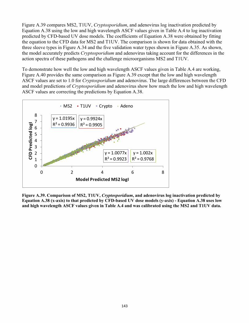
143

Figure A.39 compares MS2, T1UV, Cryptosporidium, and adenovirus log inactivation predicted by Equation A.38 using the low and high wavelength ASCF values given in Table A.4 to log inactivation predicted by CFD-based UV dose models. The coefficients of Equation A.38 were obtained by fitting the equation to the CFD data for MS2 and T1UV. The comparison is shown for data obtained with the three sleeve types in Figure A.34 and the five validation water types shown in Figure A.35. As shown, the model accurately predicts Cryptosporidium and adenovirus taking account for the differences in the action spectra of these pathogens and the challenge microorganisms MS2 and T1UV.

To demonstrate how well the low and high wavelength ASCF values given in Table A.4 are working, Figure A.40 provides the same comparison as Figure A.39 except that the low and high wavelength ASCF values are set to 1.0 for Cryptosporidium and adenovirus. The large differences between the CFD and model predictions of Cryptosporidium and adenovirus show how much the low and high wavelength ASCF values are correcting the predictions by Equation A.38.

y = 1.0195xR² = 0.9936

y = 0.9924xR² = 0.9905

y = 1.0077xR² = 0.9923

y = 1.002xR² = 0.9768

012345678

0 2 4 6 8

CFD

Pred

icte

d lo

gI


MS2 T1UV Crypto Adeno

Figure A.39. Comparison of MS2, T1UV, Cryptosporidium, and adenovirus log inactivation predicted by Equation A.38 (x-axis) to that predicted by CFD-based UV dose models (y-axis) - Equation A.38 uses low and high wavelength ASCF values given in Table A.4 and was calibrated using the MS2 and T1UV data.

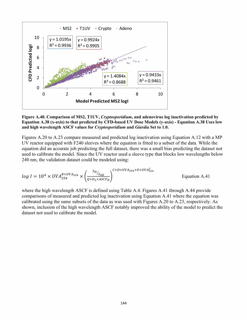
144

y = 1.0195xR² = 0.9936

y = 0.9924xR² = 0.9905

y = 0.9433xR² = 0.9461

y = 1.4084xR² = 0.8688

0

2

4

6

8

10

0 2 4 6 8 10

CFD

Pred

icte

d lo

gI


MS2 T1UV Crypto Adeno

Figure A.40. Comparison of MS2, T1UV, Cryptosporidium, and adenovirus log inactivation predicted by Equation A.38 (x-axis) to that predicted by CFD-based UV Dose Models (y-axis) - Equation A.38 Uses low and high wavelength ASCF values for Cryptosporidium and Giardia Set to 1.0.

Figures A.20 to A.23 compare measured and predicted log inactivation using Equation A.12 with a MP UV reactor equipped with F240 sleeves where the equation is fitted to a subset of the data. While the equation did an accurate job predicting the full dataset, there was a small bias predicting the dataset not used to calibrate the model. Since the UV reactor used a sleeve type that blocks low wavelengths below 240 nm, the validation dataset could be modeled using:




Equation A.41

where the high wavelength ASCF is defined using Table A.4. Figures A.41 through A.44 provide comparisons of measured and predicted log inactivation using Equation A.41 where the equation was calibrated using the same subsets of the data as was used with Figures A.20 to A.23, respectively. As shown, inclusion of the high wavelength ASCF notably improved the ability of the model to predict the dataset not used to calibrate the model.

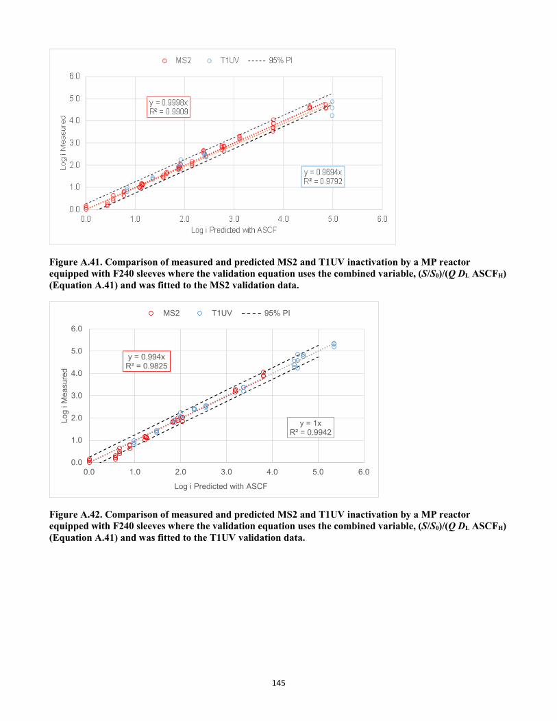
145

Figure A.41. Comparison of measured and predicted MS2 and T1UV inactivation by a MP reactor equipped with F240 sleeves where the validation equation uses the combined variable, (S/S0)/(Q DL ASCFH) (Equation A.41) and was fitted to the MS2 validation data.

y = 0.994xR² = 0.9825

y = 1xR² = 0.9942

0.0

1.0

2.0

3.0

4.0

5.0

6.0

0.0 1.0 2.0 3.0 4.0 5.0 6.0

Log

i Mea

sure

d

Log i Predicted with ASCF

MS2 T1UV 95% PI

Figure A.42. Comparison of measured and predicted MS2 and T1UV inactivation by a MP reactor equipped with F240 sleeves where the validation equation uses the combined variable, (S/S0)/(Q DL ASCFH) (Equation A.41) and was fitted to the T1UV validation data.

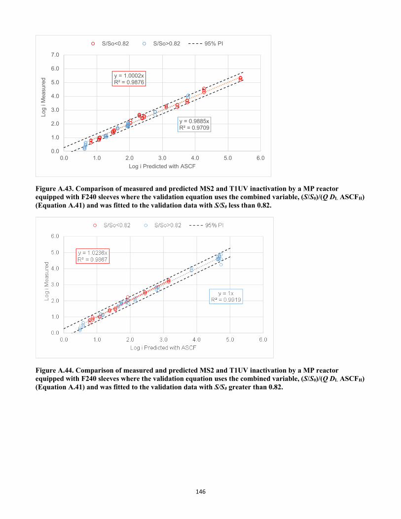
146

y = 1.0002xR² = 0.9876

y = 0.9885xR² = 0.9709

0.0

1.0

2.0

3.0

4.0

5.0

6.0

7.0

0.0 1.0 2.0 3.0 4.0 5.0 6.0

Log

i Mea

sure

d

Log i Predicted with ASCF

S/So<0.82 S/So>0.82 95% PI

Figure A.43. Comparison of measured and predicted MS2 and T1UV inactivation by a MP reactor equipped with F240 sleeves where the validation equation uses the combined variable, (S/S0)/(Q DL ASCFH) (Equation A.41) and was fitted to the validation data with S/S0 less than 0.82.

Figure A.44. Comparison of measured and predicted MS2 and T1UV inactivation by a MP reactor equipped with F240 sleeves where the validation equation uses the combined variable, (S/S0)/(Q DL ASCFH) (Equation A.41) and was fitted to the validation data with S/S0 greater than 0.82.

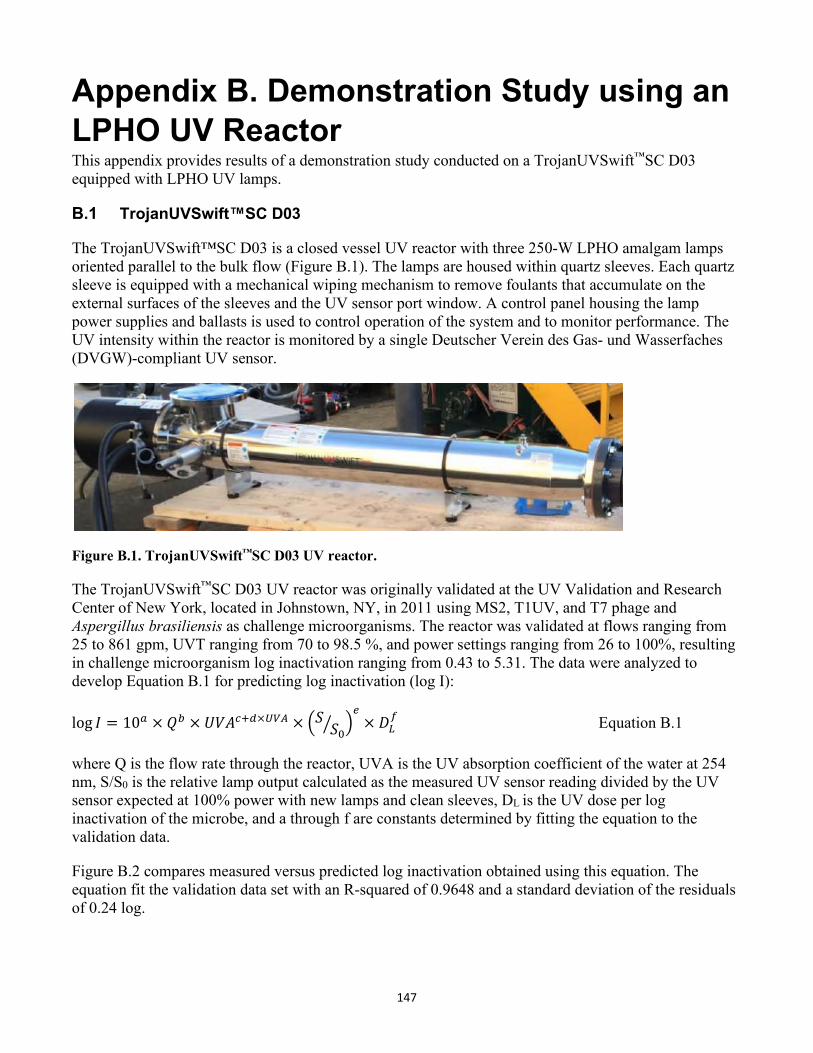
147

Appendix B. Demonstration Study using an LPHO UV Reactor This appendix provides results of a demonstration study conducted on a TrojanUVSwift™SC D03 equipped with LPHO UV lamps.

B.1 TrojanUVSwift™SC D03

The TrojanUVSwift™SC D03 is a closed vessel UV reactor with three 250-W LPHO amalgam lamps oriented parallel to the bulk flow (Figure B.1). The lamps are housed within quartz sleeves. Each quartz sleeve is equipped with a mechanical wiping mechanism to remove foulants that accumulate on the external surfaces of the sleeves and the UV sensor port window. A control panel housing the lamp power supplies and ballasts is used to control operation of the system and to monitor performance. The UV intensity within the reactor is monitored by a single Deutscher Verein des Gas- und Wasserfaches (DVGW)-compliant UV sensor.

Figure B.1. TrojanUVSwift™SC D03 UV reactor.

The TrojanUVSwift™SC D03 UV reactor was originally validated at the UV Validation and Research Center of New York, located in Johnstown, NY, in 2011 using MS2, T1UV, and T7 phage and Aspergillus brasiliensis as challenge microorganisms. The reactor was validated at flows ranging from 25 to 861 gpm, UVT ranging from 70 to 98.5 %, and power settings ranging from 26 to 100%, resulting in challenge microorganism log inactivation ranging from 0.43 to 5.31. The data were analyzed to develop Equation B.1 for predicting log inactivation (log I):

log 𝐼𝐼 = 10𝑎𝑎 × 𝑄𝑄𝑏𝑏 × 𝑈𝑈𝑉𝑉𝐴𝐴𝑐𝑐+𝑑𝑑×𝑈𝑈𝑈𝑈𝐴𝐴 × �𝑆𝑆 𝑆𝑆0� �𝑒𝑒

× 𝐷𝐷𝐿𝐿𝑓𝑓 Equation B.1

where Q is the flow rate through the reactor, UVA is the UV absorption coefficient of the water at 254 nm, S/S0 is the relative lamp output calculated as the measured UV sensor reading divided by the UV sensor expected at 100% power with new lamps and clean sleeves, DL is the UV dose per log inactivation of the microbe, and a through f are constants determined by fitting the equation to the validation data.

Figure B.2 compares measured versus predicted log inactivation obtained using this equation. The equation fit the validation data set with an R-squared of 0.9648 and a standard deviation of the residuals of 0.24 log.

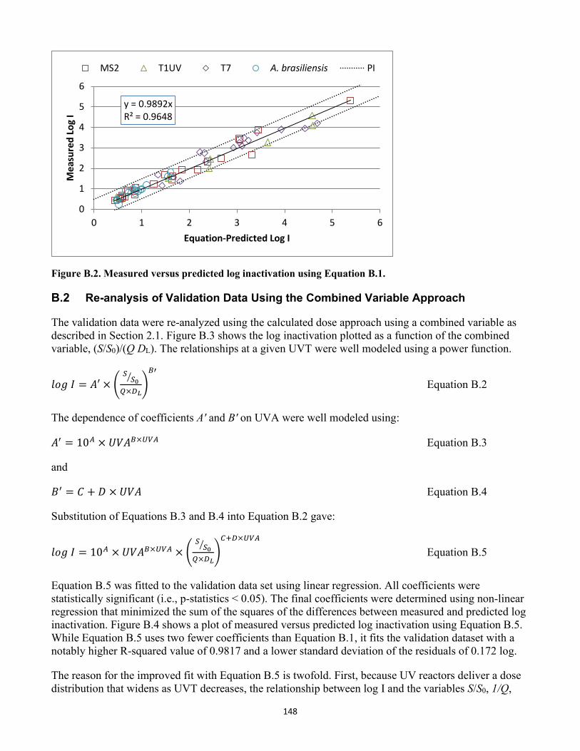
148

y = 0.9892xR² = 0.9648

0

1

2

3

4

5

6

0 1 2 3 4 5 6

Mea

sure

d Lo

g I



Figure B.2. Measured versus predicted log inactivation using Equation B.1.

B.2 Re-analysis of Validation Data Using the Combined Variable Approach

The validation data were re-analyzed using the calculated dose approach using a combined variable as described in Section 2.1. Figure B.3 shows the log inactivation plotted as a function of the combined variable, (S/S0)/(Q DL). The relationships at a given UVT were well modeled using a power function.



Equation B.2

The dependence of coefficients A' and B' on UVA were well modeled using:

𝐴𝐴′ = 10𝐴𝐴 × 𝑈𝑈𝑉𝑉𝐴𝐴𝐵𝐵×𝑈𝑈𝑈𝑈𝐴𝐴 Equation B.3

and

𝐵𝐵′ = 𝐴𝐴 + 𝐷𝐷 × 𝑈𝑈𝑉𝑉𝐴𝐴 Equation B.4

Substitution of Equations B.3 and B.4 into Equation B.2 gave:



Equation B.5

Equation B.5 was fitted to the validation data set using linear regression. All coefficients were statistically significant (i.e., p-statistics < 0.05). The final coefficients were determined using non-linear regression that minimized the sum of the squares of the differences between measured and predicted log inactivation. Figure B.4 shows a plot of measured versus predicted log inactivation using Equation B.5. While Equation B.5 uses two fewer coefficients than Equation B.1, it fits the validation dataset with a notably higher R-squared value of 0.9817 and a lower standard deviation of the residuals of 0.172 log.

The reason for the improved fit with Equation B.5 is twofold. First, because UV reactors deliver a dose distribution that widens as UVT decreases, the relationship between log I and the variables S/S0, 1/Q,

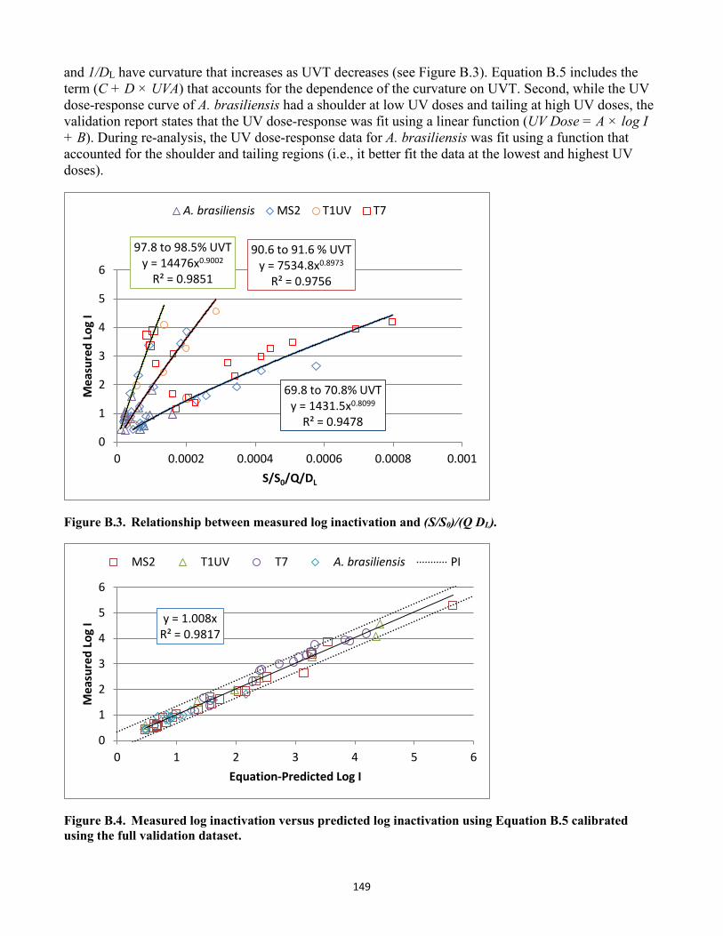
149

and 1/DL have curvature that increases as UVT decreases (see Figure B.3). Equation B.5 includes the term (C + D × UVA) that accounts for the dependence of the curvature on UVT. Second, while the UV dose-response curve of A. brasiliensis had a shoulder at low UV doses and tailing at high UV doses, the validation report states that the UV dose-response was fit using a linear function (UV Dose = A × log I + B). During re-analysis, the UV dose-response data for A. brasiliensis was fit using a function thataccounted for the shoulder and tailing regions (i.e., it better fit the data at the lowest and highest UVdoses).

69.8 to 70.8% UVTy = 1431.5x0.8099

R² = 0.9478

90.6 to 91.6 % UVTy = 7534.8x0.8973

R² = 0.9756

97.8 to 98.5% UVTy = 14476x0.9002

R² = 0.9851

0

1

2

3

4

5

6

0 0.0002 0.0004 0.0006 0.0008 0.001

Mea

sure

d Lo

g I

S/S0/Q/DL

A. brasiliensis MS2 T1UV T7

Figure B.3. Relationship between measured log inactivation and (S/S0)/(Q DL).

y = 1.008xR² = 0.9817

0

1

2

3

4

5

6

0 1 2 3 4 5 6

Mea

sure

d Lo

g I



Figure B.4. Measured log inactivation versus predicted log inactivation using Equation B.5 calibrated using the full validation dataset.

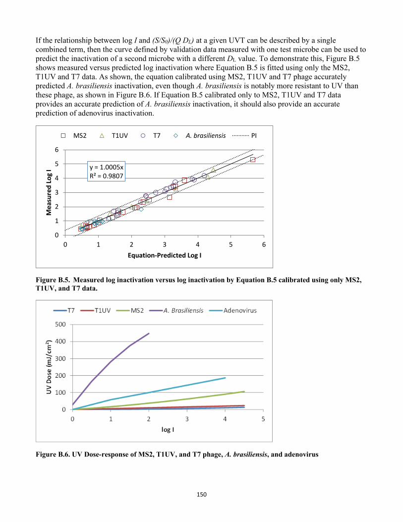
150

If the relationship between log I and (S/S0)/(Q DL) at a given UVT can be described by a single combined term, then the curve defined by validation data measured with one test microbe can be used to predict the inactivation of a second microbe with a different DL value. To demonstrate this, Figure B.5 shows measured versus predicted log inactivation where Equation B.5 is fitted using only the MS2, T1UV and T7 data. As shown, the equation calibrated using MS2, T1UV and T7 phage accurately predicted A. brasiliensis inactivation, even though A. brasiliensis is notably more resistant to UV than these phage, as shown in Figure B.6. If Equation B.5 calibrated only to MS2, T1UV and T7 data provides an accurate prediction of A. brasiliensis inactivation, it should also provide an accurate prediction of adenovirus inactivation.

y = 1.0005xR² = 0.9807

0

1

2

3

4

5

6

0 1 2 3 4 5 6

Mea

sure

d Lo

g I



Figure B.5. Measured log inactivation versus log inactivation by Equation B.5 calibrated using only MS2, T1UV, and T7 data.

Figure B.6. UV Dose-response of MS2, T1UV, and T7 phage, A. brasiliensis, and adenovirus

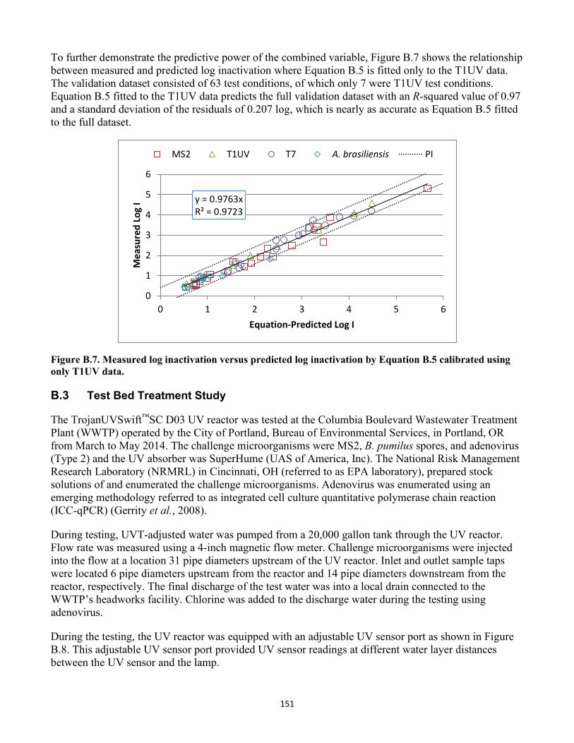
151

To further demonstrate the predictive power of the combined variable, Figure B.7 shows the relationship between measured and predicted log inactivation where Equation B.5 is fitted only to the T1UV data. The validation dataset consisted of 63 test conditions, of which only 7 were T1UV test conditions. Equation B.5 fitted to the T1UV data predicts the full validation dataset with an R-squared value of 0.97 and a standard deviation of the residuals of 0.207 log, which is nearly as accurate as Equation B.5 fitted to the full dataset.

y = 0.9763xR² = 0.9723

0

1

2

3

4

5

6

0 1 2 3 4 5 6

Mea

sure

d Lo

g I



Figure B.7. Measured log inactivation versus predicted log inactivation by Equation B.5 calibrated using only T1UV data.

B.3 Test Bed Treatment Study

The TrojanUVSwift™SC D03 UV reactor was tested at the Columbia Boulevard Wastewater Treatment Plant (WWTP) operated by the City of Portland, Bureau of Environmental Services, in Portland, OR from March to May 2014. The challenge microorganisms were MS2, B. pumilus spores, and adenovirus (Type 2) and the UV absorber was SuperHume (UAS of America, Inc). The National Risk Management Research Laboratory (NRMRL) in Cincinnati, OH (referred to as EPA laboratory), prepared stock solutions of and enumerated the challenge microorganisms. Adenovirus was enumerated using an emerging methodology referred to as integrated cell culture quantitative polymerase chain reaction (ICC-qPCR) (Gerrity et al., 2008).

During testing, UVT-adjusted water was pumped from a 20,000 gallon tank through the UV reactor. Flow rate was measured using a 4-inch magnetic flow meter. Challenge microorganisms were injected into the flow at a location 31 pipe diameters upstream of the UV reactor. Inlet and outlet sample taps were located 6 pipe diameters upstream from the reactor and 14 pipe diameters downstream from the reactor, respectively. The final discharge of the test water was into a local drain connected to the WWTP’s headworks facility. Chlorine was added to the discharge water during the testing using adenovirus.

During the testing, the UV reactor was equipped with an adjustable UV sensor port as shown in Figure B.8. This adjustable UV sensor port provided UV sensor readings at different water layer distances between the UV sensor and the lamp.

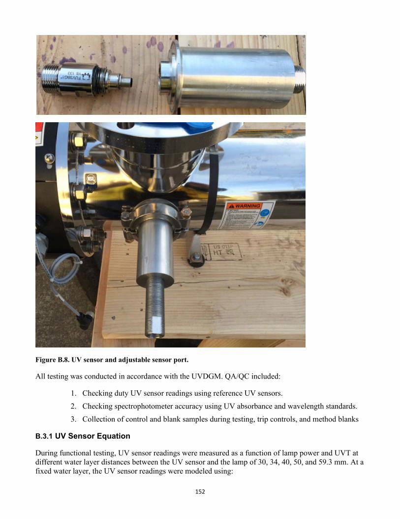
152

Figure B.8. UV sensor and adjustable sensor port.

All testing was conducted in accordance with the UVDGM. QA/QC included:

1. Checking duty UV sensor readings using reference UV sensors.2. Checking spectrophotometer accuracy using UV absorbance and wavelength standards.3. Collection of control and blank samples during testing, trip controls, and method blanks

B.3.1 UV Sensor Equation

During functional testing, UV sensor readings were measured as a function of lamp power and UVT at different water layer distances between the UV sensor and the lamp of 30, 34, 40, 50, and 59.3 mm. At a fixed water layer, the UV sensor readings were modeled using:

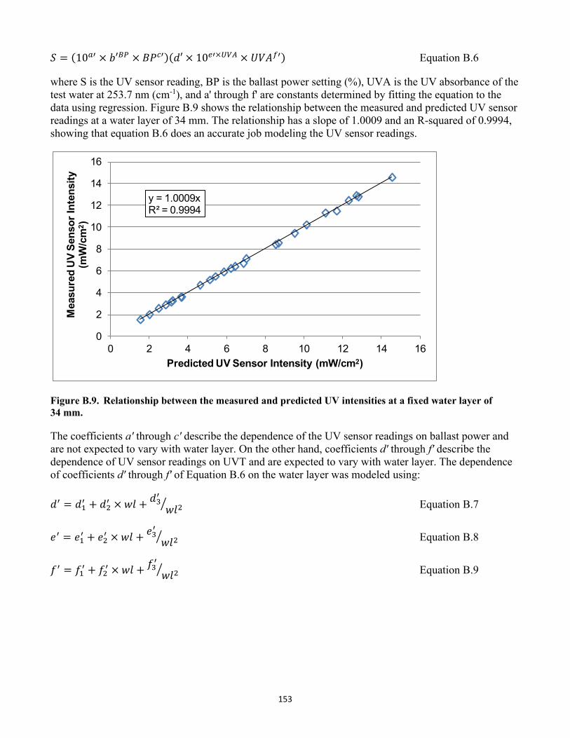
153

𝑆𝑆 = (10𝑎𝑎′ × 𝑏𝑏′𝐵𝐵𝑃𝑃 × 𝐵𝐵𝑃𝑃𝑐𝑐′)(𝑉𝑉′ × 10𝑒𝑒′×𝑈𝑈𝑈𝑈𝐴𝐴 × 𝑈𝑈𝑉𝑉𝐴𝐴𝑓𝑓′) Equation B.6

where S is the UV sensor reading, BP is the ballast power setting (%), UVA is the UV absorbance of the test water at 253.7 nm (cm-1), and a' through f' are constants determined by fitting the equation to the data using regression. Figure B.9 shows the relationship between the measured and predicted UV sensor readings at a water layer of 34 mm. The relationship has a slope of 1.0009 and an R-squared of 0.9994, showing that equation B.6 does an accurate job modeling the UV sensor readings.

y = 1.0009xR² = 0.9994

0

2

4

6

8

10

12

14

16

0 2 4 6 8 10 12 14 16

Mea

sure

d U

V Se

nsor

Inte

nsity

(m

W/c

m2 )

Predicted UV Sensor Intensity (mW/cm2)

Figure B.9. Relationship between the measured and predicted UV intensities at a fixed water layer of 34 mm.

The coefficients a' through c' describe the dependence of the UV sensor readings on ballast power and are not expected to vary with water layer. On the other hand, coefficients d' through f' describe the dependence of UV sensor readings on UVT and are expected to vary with water layer. The dependence of coefficients d' through f' of Equation B.6 on the water layer was modeled using:

𝑉𝑉′ = 𝑉𝑉1′ + 𝑉𝑉2′ × 𝑤𝑤𝑉𝑉 + 𝑉𝑉3′𝑤𝑤𝑉𝑉2� Equation B.7

𝑡𝑡′ = 𝑡𝑡1′ + 𝑡𝑡2′ × 𝑤𝑤𝑉𝑉 + 𝑡𝑡3′𝑤𝑤𝑉𝑉2� Equation B.8

𝑓𝑓′ = 𝑓𝑓1′ + 𝑓𝑓2′ × 𝑤𝑤𝑉𝑉 + 𝑓𝑓3′𝑤𝑤𝑉𝑉2� Equation B.9

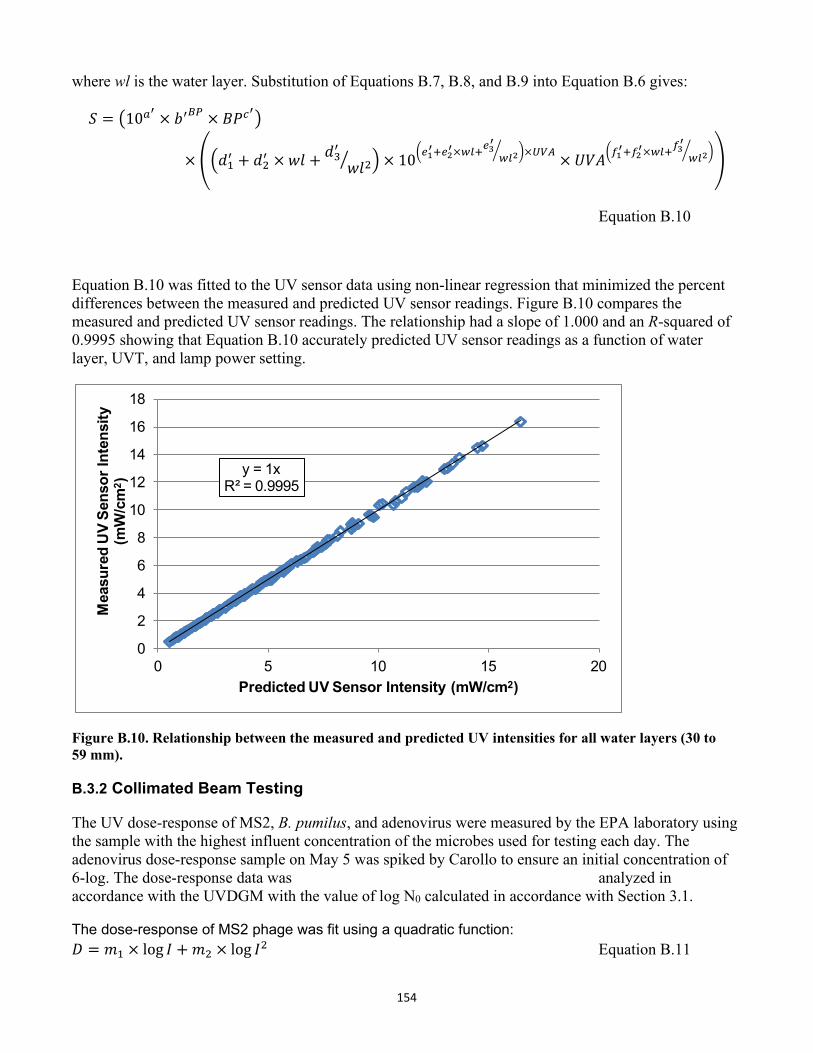
154

where wl is the water layer. Substitution of Equations B.7, B.8, and B.9 into Equation B.6 gives:

𝑆𝑆 = �10𝑎𝑎′ × 𝑏𝑏′𝐵𝐵𝑃𝑃 × 𝐵𝐵𝑃𝑃𝑐𝑐′�

× ��𝑉𝑉1′ + 𝑉𝑉2′ × 𝑤𝑤𝑉𝑉 + 𝑉𝑉3′𝑤𝑤𝑉𝑉2� � × 10�𝑒𝑒1

′+𝑒𝑒2′×𝐿𝐿𝑃𝑃+𝑒𝑒3′

𝐿𝐿𝑃𝑃2� �×𝑈𝑈𝑈𝑈𝐴𝐴 × 𝑈𝑈𝑉𝑉𝐴𝐴�𝑓𝑓1

′+𝑓𝑓2′×𝐿𝐿𝑃𝑃+𝑓𝑓3′

𝐿𝐿𝑃𝑃2� ��

Equation B.10

Equation B.10 was fitted to the UV sensor data using non-linear regression that minimized the percent differences between the measured and predicted UV sensor readings. Figure B.10 compares the measured and predicted UV sensor readings. The relationship had a slope of 1.000 and an R-squared of 0.9995 showing that Equation B.10 accurately predicted UV sensor readings as a function of water layer, UVT, and lamp power setting.

y = 1xR² = 0.9995

0

2

4

6

8

10

12

14

16

18

0 5 10 15 20

Mea

sure

d U

V Se

nsor

Inte

nsity

(m

W/c

m2 )

Predicted UV Sensor Intensity (mW/cm2)

Figure B.10. Relationship between the measured and predicted UV intensities for all water layers (30 to 59 mm).

B.3.2 Collimated Beam Testing

The UV dose-response of MS2, B. pumilus, and adenovirus were measured by the EPA laboratory using the sample with the highest influent concentration of the microbes used for testing each day. The adenovirus dose-response sample on May 5 was spiked by Carollo to ensure an initial concentration of 6-log. The dose-response data was analyzed in accordance with the UVDGM with the value of log N0 calculated in accordance with Section 3.1.

The dose-response of MS2 phage was fit using a quadratic function: 𝐷𝐷 = 𝑚𝑚1 × log 𝐼𝐼 + 𝑚𝑚2 × log 𝐼𝐼2 Equation B.11

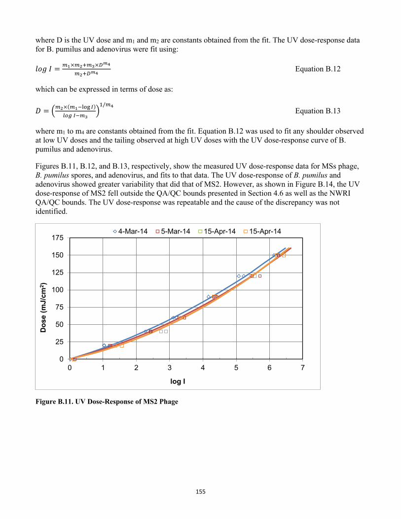
155

where D is the UV dose and m1 and m2 are constants obtained from the fit. The UV dose-response data for B. pumilus and adenovirus were fit using:

𝑉𝑉𝐷𝐷𝑙𝑙 𝐼𝐼 = 𝑛𝑛1×𝑛𝑛2+𝑛𝑛3×𝑅𝑅𝑛𝑛4

𝑛𝑛2+𝑅𝑅𝑛𝑛4Equation B.12

which can be expressed in terms of dose as:

𝐷𝐷 = �𝑛𝑛2×(𝑛𝑛1−log 𝐼𝐼)𝑃𝑃𝑃𝑃𝐴𝐴 𝐼𝐼−𝑛𝑛3

�1/𝑛𝑛4

Equation B.13

where m1 to m4 are constants obtained from the fit. Equation B.12 was used to fit any shoulder observed at low UV doses and the tailing observed at high UV doses with the UV dose-response curve of B. pumilus and adenovirus.

Figures B.11, B.12, and B.13, respectively, show the measured UV dose-response data for MSs phage, B. pumilus spores, and adenovirus, and fits to that data. The UV dose-response of B. pumilus andadenovirus showed greater variability that did that of MS2. However, as shown in Figure B.14, the UVdose-response of MS2 fell outside the QA/QC bounds presented in Section 4.6 as well as the NWRIQA/QC bounds. The UV dose-response was repeatable and the cause of the discrepancy was notidentified.

0

25

50

75

100

125

150

175

0 1 2 3 4 5 6 7

Dose

(mJ/

cm2 )

log I

4-Mar-14 5-Mar-14 15-Apr-14 15-Apr-14

Figure B.11. UV Dose-Response of MS2 Phage

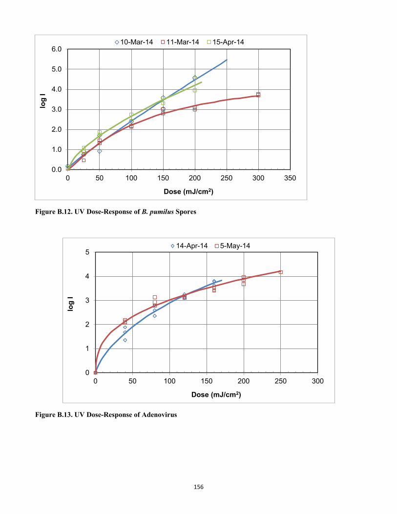
156

0.0

1.0

2.0

3.0

4.0

5.0

6.0

0 50 100 150 200 250 300 350

log

I

Dose (mJ/cm2)

10-Mar-14 11-Mar-14 15-Apr-14

Figure B.12. UV Dose-Response of B. pumilus Spores

0

1

2

3

4

5

0 50 100 150 200 250 300

log

I

Dose (mJ/cm2)

14-Apr-14 5-May-14

Figure B.13. UV Dose-Response of Adenovirus

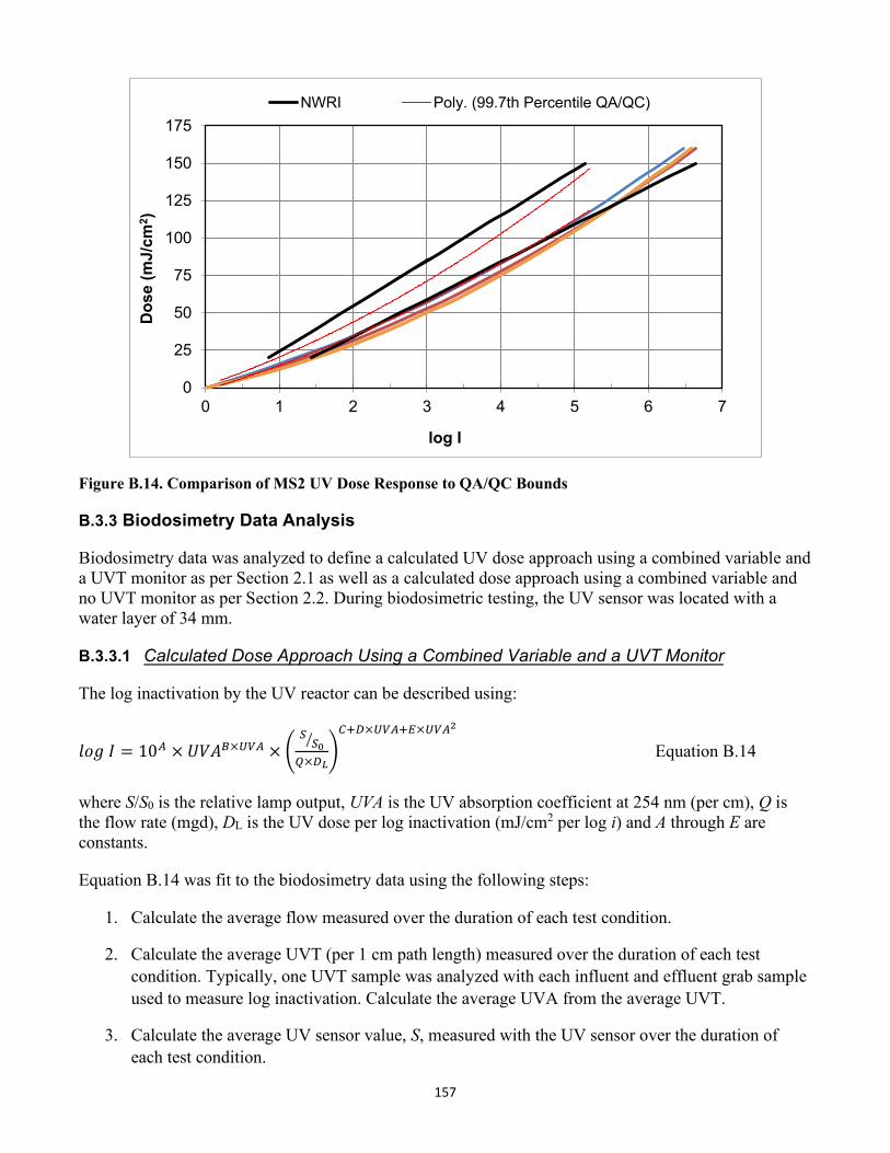
157

0

25

50

75

100

125

150

175

0 1 2 3 4 5 6 7

Dose

(mJ/

cm2 )

log I

NWRI Poly. (99.7th Percentile QA/QC)

Figure B.14. Comparison of MS2 UV Dose Response to QA/QC Bounds

B.3.3 Biodosimetry Data Analysis

Biodosimetry data was analyzed to define a calculated UV dose approach using a combined variable and a UVT monitor as per Section 2.1 as well as a calculated dose approach using a combined variable and no UVT monitor as per Section 2.2. During biodosimetric testing, the UV sensor was located with a water layer of 34 mm.

B.3.3.1 Calculated Dose Approach Using a Combined Variable and a UVT Monitor

The log inactivation by the UV reactor can be described using:



Equation B.14

where S/S0 is the relative lamp output, UVA is the UV absorption coefficient at 254 nm (per cm), Q is the flow rate (mgd), DL is the UV dose per log inactivation (mJ/cm2 per log i) and A through E are constants.

Equation B.14 was fit to the biodosimetry data using the following steps:

1. Calculate the average flow measured over the duration of each test condition.

2. Calculate the average UVT (per 1 cm path length) measured over the duration of each testcondition. Typically, one UVT sample was analyzed with each influent and effluent grab sampleused to measure log inactivation. Calculate the average UVA from the average UVT.

3. Calculate the average UV sensor value, S, measured with the UV sensor over the duration ofeach test condition.

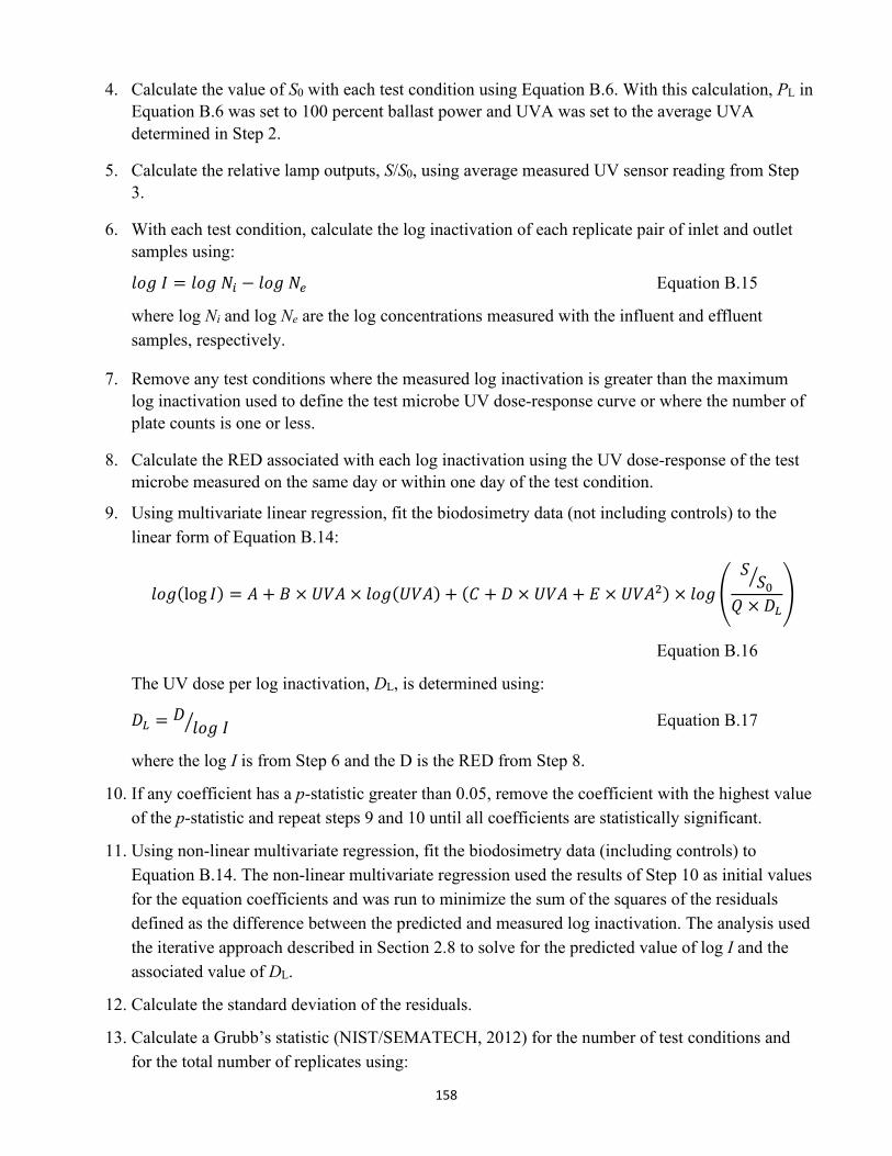
158

4. Calculate the value of S0 with each test condition using Equation B.6. With this calculation, PL inEquation B.6 was set to 100 percent ballast power and UVA was set to the average UVAdetermined in Step 2.

5. Calculate the relative lamp outputs, S/S0, using average measured UV sensor reading from Step3.

6. With each test condition, calculate the log inactivation of each replicate pair of inlet and outletsamples using:

𝑉𝑉𝐷𝐷𝑙𝑙 𝐼𝐼 = 𝑉𝑉𝐷𝐷𝑙𝑙 𝑁𝑁𝑀𝑀 − 𝑉𝑉𝐷𝐷𝑙𝑙 𝑁𝑁𝑒𝑒 Equation B.15

where log Ni and log Ne are the log concentrations measured with the influent and effluentsamples, respectively.

7. Remove any test conditions where the measured log inactivation is greater than the maximumlog inactivation used to define the test microbe UV dose-response curve or where the number ofplate counts is one or less.

8. Calculate the RED associated with each log inactivation using the UV dose-response of the testmicrobe measured on the same day or within one day of the test condition.

9. Using multivariate linear regression, fit the biodosimetry data (not including controls) to thelinear form of Equation B.14:

𝑉𝑉𝐷𝐷𝑙𝑙(log 𝐼𝐼) = 𝐴𝐴 + 𝐵𝐵 × 𝑈𝑈𝑉𝑉𝐴𝐴 × 𝑉𝑉𝐷𝐷𝑙𝑙(𝑈𝑈𝑉𝑉𝐴𝐴) + (𝐴𝐴 + 𝐷𝐷 × 𝑈𝑈𝑉𝑉𝐴𝐴 + 𝑅𝑅 × 𝑈𝑈𝑉𝑉𝐴𝐴2) × 𝑉𝑉𝐷𝐷𝑙𝑙 �𝑆𝑆𝑆𝑆0�

𝑄𝑄 × 𝐷𝐷𝐿𝐿�

Equation B.16

The UV dose per log inactivation, DL, is determined using:

𝐷𝐷𝐿𝐿 = 𝐷𝐷𝑉𝑉𝐷𝐷𝑙𝑙 𝐼𝐼� Equation B.17

where the log I is from Step 6 and the D is the RED from Step 8.

10. If any coefficient has a p-statistic greater than 0.05, remove the coefficient with the highest valueof the p-statistic and repeat steps 9 and 10 until all coefficients are statistically significant.

11. Using non-linear multivariate regression, fit the biodosimetry data (including controls) toEquation B.14. The non-linear multivariate regression used the results of Step 10 as initial valuesfor the equation coefficients and was run to minimize the sum of the squares of the residualsdefined as the difference between the predicted and measured log inactivation. The analysis usedthe iterative approach described in Section 2.8 to solve for the predicted value of log I and theassociated value of DL.

12. Calculate the standard deviation of the residuals.

13. Calculate a Grubb’s statistic (NIST/SEMATECH, 2012) for the number of test conditions andfor the total number of replicates using:

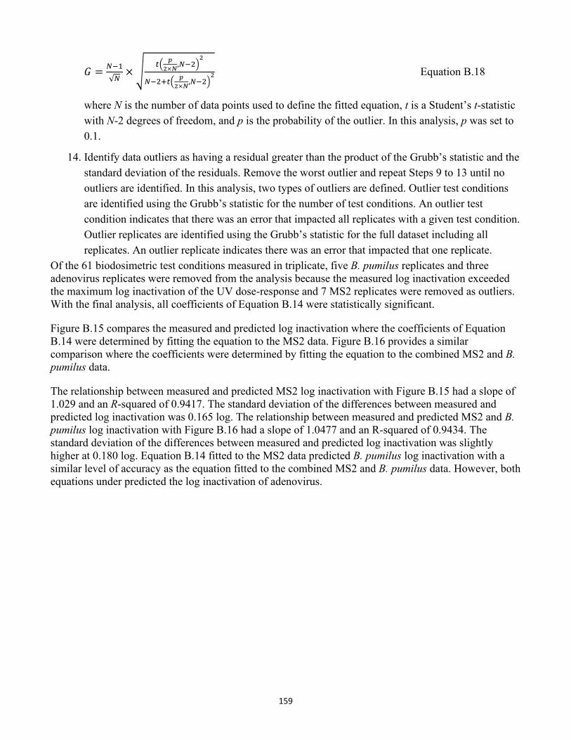
159

𝐺𝐺 = 𝐼𝐼−1√𝐼𝐼

× �𝑡𝑡� 𝑝𝑝2×𝑙𝑙,𝐼𝐼−2�

2

𝐼𝐼−2+𝑡𝑡� 𝑝𝑝2×𝑙𝑙,𝐼𝐼−2�

2 Equation B.18

where N is the number of data points used to define the fitted equation, t is a Student’s t-statistic with N-2 degrees of freedom, and p is the probability of the outlier. In this analysis, p was set to 0.1.

14. Identify data outliers as having a residual greater than the product of the Grubb’s statistic and thestandard deviation of the residuals. Remove the worst outlier and repeat Steps 9 to 13 until nooutliers are identified. In this analysis, two types of outliers are defined. Outlier test conditionsare identified using the Grubb’s statistic for the number of test conditions. An outlier testcondition indicates that there was an error that impacted all replicates with a given test condition.Outlier replicates are identified using the Grubb’s statistic for the full dataset including allreplicates. An outlier replicate indicates there was an error that impacted that one replicate.

Of the 61 biodosimetric test conditions measured in triplicate, five B. pumilus replicates and three adenovirus replicates were removed from the analysis because the measured log inactivation exceeded the maximum log inactivation of the UV dose-response and 7 MS2 replicates were removed as outliers. With the final analysis, all coefficients of Equation B.14 were statistically significant.

Figure B.15 compares the measured and predicted log inactivation where the coefficients of Equation B.14 were determined by fitting the equation to the MS2 data. Figure B.16 provides a similarcomparison where the coefficients were determined by fitting the equation to the combined MS2 and B.pumilus data.

The relationship between measured and predicted MS2 log inactivation with Figure B.15 had a slope of 1.029 and an R-squared of 0.9417. The standard deviation of the differences between measured and predicted log inactivation was 0.165 log. The relationship between measured and predicted MS2 and B. pumilus log inactivation with Figure B.16 had a slope of 1.0477 and an R-squared of 0.9434. The standard deviation of the differences between measured and predicted log inactivation was slightly higher at 0.180 log. Equation B.14 fitted to the MS2 data predicted B. pumilus log inactivation with a similar level of accuracy as the equation fitted to the combined MS2 and B. pumilus data. However, both equations under predicted the log inactivation of adenovirus.

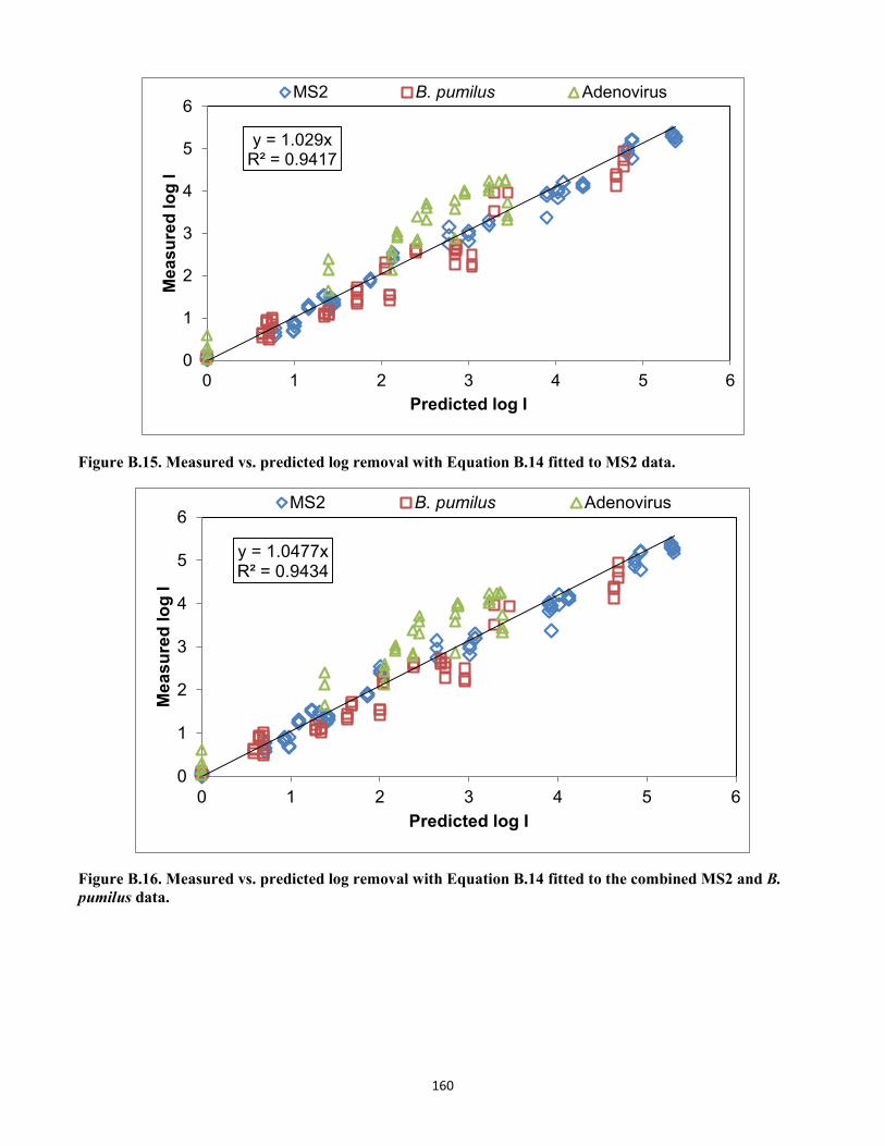
160

y = 1.029xR² = 0.9417

0

1

2

3

4

5

6

0 1 2 3 4 5 6

Mea

sure

d lo

g I

Predicted log I

MS2 B. pumilus Adenovirus

Figure B.15. Measured vs. predicted log removal with Equation B.14 fitted to MS2 data.

y = 1.0477xR² = 0.9434

0

1

2

3

4

5

6

0 1 2 3 4 5 6

Mea

sure

d lo

g I

Predicted log I

MS2 B. pumilus Adenovirus

Figure B.16. Measured vs. predicted log removal with Equation B.14 fitted to the combined MS2 and B. pumilus data.

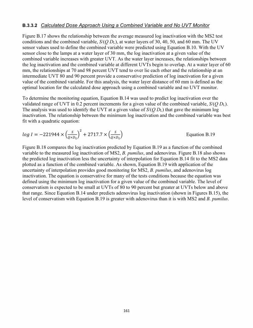
161

B.3.3.2 Calculated Dose Approach Using a Combined Variable and No UVT Monitor

Figure B.17 shows the relationship between the average measured log inactivation with the MS2 test conditions and the combined variable, S/(Q DL), at water layers of 30, 40, 50, and 60 mm. The UV sensor values used to define the combined variable were predicted using Equation B.10. With the UV sensor close to the lamps at a water layer of 30 mm, the log inactivation at a given value of the combined variable increases with greater UVT. As the water layer increases, the relationships between the log inactivation and the combined variable at different UVTs begin to overlap. At a water layer of 60 mm, the relationships at 70 and 98 percent UVT tend to over lie each other and the relationship at an intermediate UVT 80 and 90 percent provide a conservative prediction of log inactivation for a given value of the combined variable. For this analysis, the water layer distance of 60 mm is defined as the optimal location for the calculated dose approach using a combined variable and no UVT monitor.

To determine the monitoring equation, Equation B.14 was used to predict log inactivation over the validated range of UVT in 0.2 percent increments for a given value of the combined variable, S/(Q DL). The analysis was used to identify the UVT at a given value of S/(Q DL) that gave the minimum log inactivation. The relationship between the minimum log inactivation and the combined variable was best fit with a quadratic equation:

𝑉𝑉𝐷𝐷𝑙𝑙 𝐼𝐼 = −221944 × � 𝑆𝑆𝑄𝑄×𝑅𝑅𝐿𝐿

�2

+ 2717.7 × � 𝑆𝑆𝑄𝑄×𝑅𝑅𝐿𝐿

� Equation B.19

Figure B.18 compares the log inactivation predicted by Equation B.19 as a function of the combined variable to the measured log inactivation of MS2, B. pumilus, and adenovirus. Figure B.18 also shows the predicted log inactivation less the uncertainty of interpolation for Equation B.14 fit to the MS2 data plotted as a function of the combined variable. As shown, Equation B.19 with application of the uncertainty of interpolation provides good monitoring for MS2, B. pumilus, and adenovirus log inactivation. The equation is conservative for many of the tests conditions because the equation was defined using the minimum log inactivation for a given value of the combined variable. The level of conservatism is expected to be small at UVTs of 80 to 90 percent but greater at UVTs below and above that range. Since Equation B.14 under predicts adenovirus log inactivation (shown in Figures B.15), the level of conservatism with Equation B.19 is greater with adenovirus than it is with MS2 and B. pumilus.

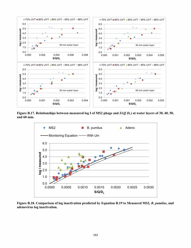
162

0.0

1.0

2.0

3.0

4.0

5.0

6.0

0.000 0.002 0.004 0.006 0.008

log

i mea

sure

d

S/Q/DL

70% UVT 80% UVT 90% UVT 95% UVT 98% UVT

30 mm water layer

0.0

1.0

2.0

3.0

4.0

5.0

6.0

0.000 0.001 0.002 0.003 0.004

log

i mea

sure

d

S/Q/DL


50 mm water layer

0.0

1.0

2.0

3.0

4.0

5.0

6.0

0.000 0.001 0.002 0.003 0.004 0.005

log

i mea

sure

d

S/Q/DL


40 mm water layer

0.0

1.0

2.0

3.0

4.0

5.0

6.0

0.000 0.001 0.001 0.002 0.002 0.003lo

g i m

easu

red

S/Q/DL


60 mm water layer

Figure B.17. Relationships between measured log I of MS2 phage and S/(Q DL) at water layers of 30, 40, 50, and 60 mm.

0.0

1.0

2.0

3.0

4.0

5.0

6.0

0.0000 0.0005 0.0010 0.0015 0.0020 0.0025 0.0030

log

i mea

sure

d

S/Q/DL

MS2 B. pumilus Adeno

Monitoring Equation With Uin

Figure B.18. Comparison of log inactivation predicted by Equation B.19 to Measured MS2, B. pumilus, and adenovirus log inactivation.

163

B.4 Discussion

One of the main objectives of this demonstration study was to show that using the combined variable approach, validation using MS2 alone can be used to predict the log inactivation of other microbes such as adenovirus, provided that they are within the validated range of the combined variable (S/S0)/(Q DL). This was initially demonstrated in Section B.2 with the analysis of the original validation data. In Section B.2, Equation B.5 fitted to T1UV log inactivation was able to accurately predict the log inactivation of A. brasiliensis despite the two order of magnitude difference between the UV sensitivities of those two microbes. This was again demonstrated during this demonstration study where MS2 log inactivation with a combined variable analysis was able to predict the log inactivation of B. pumilus despite the difference in sensitivities shown in Figures B.11 and B.12. This test bed study also showed that the combined variable approach calibrated using MS2 phage under predicted adenovirus inactivation. As shown in Figures B.16 and B.17, the measured log inactivation for adenovirus was approximately 0.5 logs greater than what is predicted through the model.

The differences in the measured and predicted log inactivation of adenovirus may be related to the integrated cell culture quantitative PCR (ICC-qPCR) technique used to enumerate adenovirus during this study. This is a new technique for the quantification of adenovirus that delivers results more quickly than traditional cell culture and could provide significant benefit to the industry. However, additional tests by the EPA lab have shown the results can be dependent on the initial concentration of the sample, which differed between the test conditions used to quantify log inactivation through the UV reactor and used to measure the UV dose-response using the collimated beam apparatus.

Analysis of biodosimetry data showed that the inclusion of B. pumilus does not help to improve the prediction of adenovirus. This observation supports the premise that using two challenge microorganisms whose UV dose response brackets that of the target pathogen is not required if the validation data is analyzed using the combined variable approach.

Last, the study demonstrates the development of a calculated dose approach that uses a combined variable without a UVT monitor. This approach is ideal for small systems because it eliminates the need to maintain an online UVT monitor.

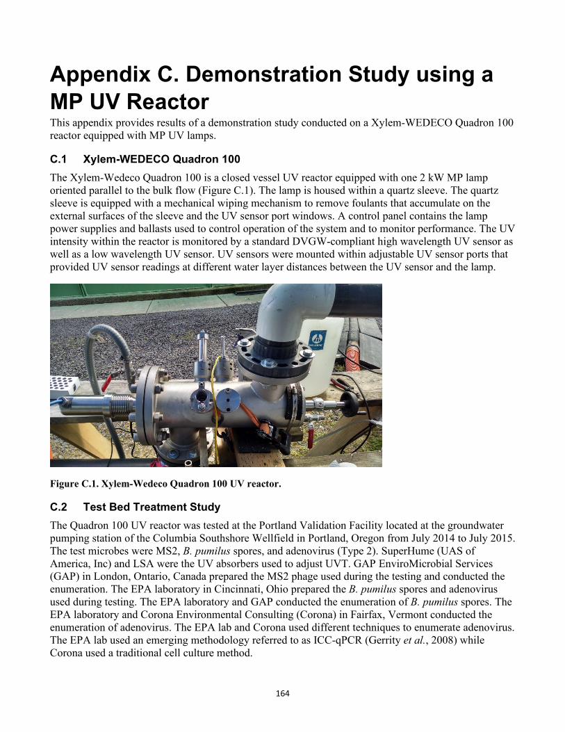
164

Appendix C. Demonstration Study using a MP UV Reactor This appendix provides results of a demonstration study conducted on a Xylem-WEDECO Quadron 100 reactor equipped with MP UV lamps.

C.1 Xylem-WEDECO Quadron 100The Xylem-Wedeco Quadron 100 is a closed vessel UV reactor equipped with one 2 kW MP lamp oriented parallel to the bulk flow (Figure C.1). The lamp is housed within a quartz sleeve. The quartz sleeve is equipped with a mechanical wiping mechanism to remove foulants that accumulate on the external surfaces of the sleeve and the UV sensor port windows. A control panel contains the lamp power supplies and ballasts used to control operation of the system and to monitor performance. The UV intensity within the reactor is monitored by a standard DVGW-compliant high wavelength UV sensor as well as a low wavelength UV sensor. UV sensors were mounted within adjustable UV sensor ports that provided UV sensor readings at different water layer distances between the UV sensor and the lamp.

Figure C.1. Xylem-Wedeco Quadron 100 UV reactor.

C.2 Test Bed Treatment StudyThe Quadron 100 UV reactor was tested at the Portland Validation Facility located at the groundwater pumping station of the Columbia Southshore Wellfield in Portland, Oregon from July 2014 to July 2015. The test microbes were MS2, B. pumilus spores, and adenovirus (Type 2). SuperHume (UAS of America, Inc) and LSA were the UV absorbers used to adjust UVT. GAP EnviroMicrobial Services (GAP) in London, Ontario, Canada prepared the MS2 phage used during the testing and conducted the enumeration. The EPA laboratory in Cincinnati, Ohio prepared the B. pumilus spores and adenovirus used during testing. The EPA laboratory and GAP conducted the enumeration of B. pumilus spores. The EPA laboratory and Corona Environmental Consulting (Corona) in Fairfax, Vermont conducted the enumeration of adenovirus. The EPA lab and Corona used different techniques to enumerate adenovirus. The EPA lab used an emerging methodology referred to as ICC-qPCR (Gerrity et al., 2008) while Corona used a traditional cell culture method.

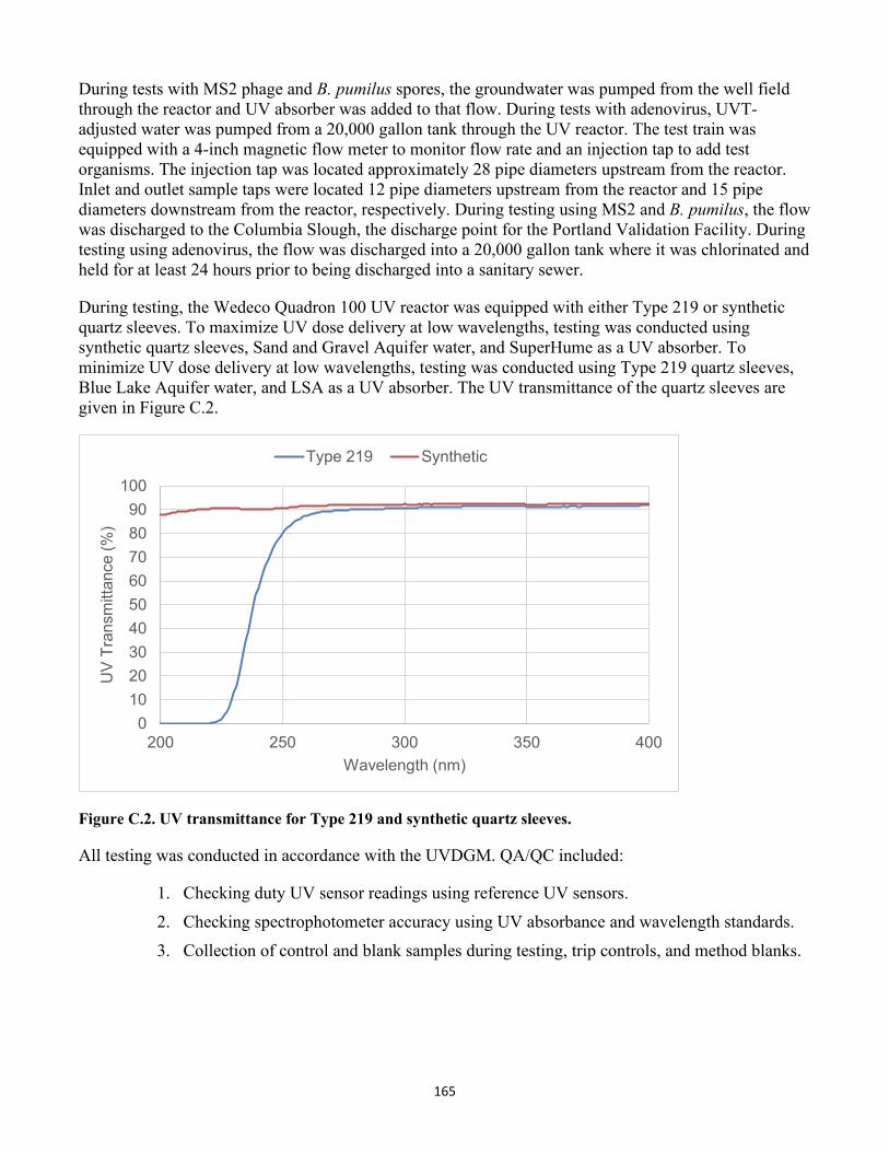
165

During tests with MS2 phage and B. pumilus spores, the groundwater was pumped from the well field through the reactor and UV absorber was added to that flow. During tests with adenovirus, UVT-adjusted water was pumped from a 20,000 gallon tank through the UV reactor. The test train was equipped with a 4-inch magnetic flow meter to monitor flow rate and an injection tap to add test organisms. The injection tap was located approximately 28 pipe diameters upstream from the reactor. Inlet and outlet sample taps were located 12 pipe diameters upstream from the reactor and 15 pipe diameters downstream from the reactor, respectively. During testing using MS2 and B. pumilus, the flow was discharged to the Columbia Slough, the discharge point for the Portland Validation Facility. During testing using adenovirus, the flow was discharged into a 20,000 gallon tank where it was chlorinated and held for at least 24 hours prior to being discharged into a sanitary sewer.

During testing, the Wedeco Quadron 100 UV reactor was equipped with either Type 219 or synthetic quartz sleeves. To maximize UV dose delivery at low wavelengths, testing was conducted using synthetic quartz sleeves, Sand and Gravel Aquifer water, and SuperHume as a UV absorber. To minimize UV dose delivery at low wavelengths, testing was conducted using Type 219 quartz sleeves, Blue Lake Aquifer water, and LSA as a UV absorber. The UV transmittance of the quartz sleeves are given in Figure C.2.

0102030405060708090

100

200 250 300 350 400

UV

Tran

smitt

ance

(%)

Wavelength (nm)

Type 219 Synthetic

Figure C.2. UV transmittance for Type 219 and synthetic quartz sleeves.

All testing was conducted in accordance with the UVDGM. QA/QC included:

1. Checking duty UV sensor readings using reference UV sensors.2. Checking spectrophotometer accuracy using UV absorbance and wavelength standards.3. Collection of control and blank samples during testing, trip controls, and method blanks.

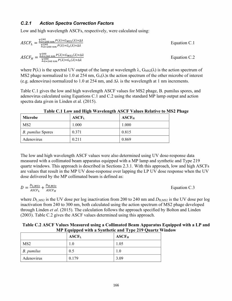
166

C.2.1 Action Spectra Correction FactorsLow and high wavelength ASCFs, respectively, were calculated using:



Equation C.1

Equation C.2

where P(λ) is the spectral UV output of the lamp at wavelength λ, GMS2(λ) is the action spectrum of MS2 phage normalized to 1.0 at 254 nm, Gx(λ)s the action spectrum of the other microbe of interest (e.g. adenovirus) normalized to 1.0 at 254 nm, and ∆λ is the wavelength at 1 nm increments.

Table C.1 gives the low and high wavelength ASCF values for MS2 phage, B. pumilus spores, and adenovirus calculated using Equations C.1 and C.2 using the standard MP lamp output and action spectra data given in Linden et al. (2015).

Table C.1 Low and High Wavelength ASCF Values Relative to MS2 Phage Microbe ASCFL ASCFH

MS2 1.000 1.000

B. pumilus Spores 0.371 0.815


The low and high wavelength ASCF values were also determined using UV dose-response data measured with a collimated beam apparatus equipped with a MP lamp and synthetic and Type 219 quartz windows. This approach is described in Sections 2.3.1. With this approach, low and high ASCFs are values that result in the MP UV dose-response over lapping the LP UV dose response when the UV dose delivered by the MP collimated beam is defined as:

𝐷𝐷 = 𝑅𝑅𝐿𝐿,𝑀𝑀𝑀𝑀2𝐴𝐴𝑆𝑆𝐶𝐶𝐹𝐹𝐿𝐿

+ 𝑅𝑅𝐻𝐻,𝑀𝑀𝑀𝑀2𝐴𝐴𝑆𝑆𝐶𝐶𝐹𝐹𝐻𝐻

Equation C.3

where DL,MS2 is the UV dose per log inactivation from 200 to 240 nm and DH,MS2 is the UV dose per log inactivation from 240 to 300 nm, both calculated using the action spectrum of MS2 phage developed through Linden et al. (2015). The calculation follows the approach specified by Bolton and Linden (2003). Table C.2 gives the ASCF values determined using this approach.

Table C.2 ASCF Values Measured using a Collimated Beam Apparatus Equipped with a LP and MP Equipped with a Synthetic and Type 219 Quartz Window

ASCFL ASCFH

MS2 1.0 1.05

B. pumilus 0.5 1.0


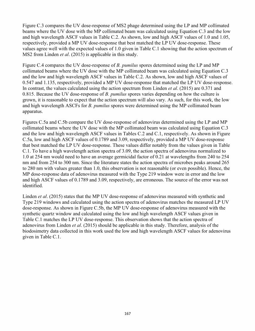
167

Figure C.3 compares the UV dose-response of MS2 phage determined using the LP and MP collimated beams where the UV dose with the MP collimated beam was calculated using Equation C.3 and the low and high wavelength ASCF values in Table C.2. As shown, low and high ASCF values of 1.0 and 1.05, respectively, provided a MP UV dose-response that best matched the LP UV dose-response. These values agree well with the expected values of 1.0 given in Table C.1 showing that the action spectrum of MS2 from Linden et al. (2015) is applicable in this study.

Figure C.4 compares the UV dose-response of B. pumilus spores determined using the LP and MP collimated beams where the UV dose with the MP collimated beam was calculated using Equation C.3 and the low and high wavelength ASCF values in Table C.2. As shown, low and high ASCF values of 0.547 and 1.135, respectively, provided a MP UV dose-response that matched the LP UV dose-response. In contrast, the values calculated using the action spectrum from Linden et al. (2015) are 0.371 and 0.815. Because the UV dose-response of B. pumilus spores varies depending on how the culture is grown, it is reasonable to expect that the action spectrum will also vary. As such, for this work, the low and high wavelength ASCFs for B. pumilus spores were determined using the MP collimated beam apparatus.

Figures C.5a and C.5b compare the UV dose-response of adenovirus determined using the LP and MP collimated beams where the UV dose with the MP collimated beam was calculated using Equation C.3 and the low and high wavelength ASCF values in Tables C.2 and C.1, respectively. As shown in Figure C.5a, low and high ASCF values of 0.1789 and 3.09, respectively, provided a MP UV dose-responsethat best matched the LP UV dose-response. These values differ notably from the values given in TableC.1. To have a high wavelength action spectra of 3.09, the action spectra of adenovirus normalized to1.0 at 254 nm would need to have an average germicidal factor of 0.21 at wavelengths from 240 to 254nm and from 254 to 300 nm. Since the literature states the action spectra of microbes peaks around 265to 280 nm with values greater than 1.0, this observation is not reasonable (or even possible). Hence, theMP dose-response data of adenovirus measured with the Type 219 window were in error and the lowand high ASCF values of 0.1789 and 3.09, respectively, are erroneous. The source of the error was notidentified.

Linden et al. (2015) states that the MP UV dose-response of adenovirus measured with synthetic and Type 219 windows and calculated using the action spectra of adenovirus matches the measured LP UV dose-response. As shown in Figure C.5b, the MP UV dose-response of adenovirus measured with the synthetic quartz window and calculated using the low and high wavelength ASCF values given in Table C.1 matches the LP UV dose-response. This observation shows that the action spectra of adenovirus from Linden et al. (2015) should be applicable in this study. Therefore, analysis of the biodosimetry data collected in this work used the low and high wavelength ASCF values for adenovirus given in Table C.1.

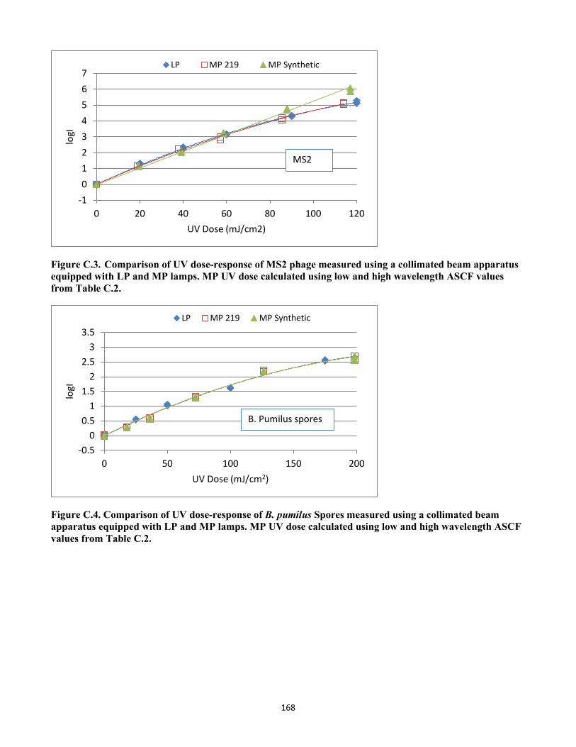
168

-101234567

0 20 40 60 80 100 120

logI

UV Dose (mJ/cm2)

LP MP 219 MP Synthetic

MS2

Figure C.3. Comparison of UV dose-response of MS2 phage measured using a collimated beam apparatus equipped with LP and MP lamps. MP UV dose calculated using low and high wavelength ASCF values from Table C.2.

-0.50

0.51

1.52

2.53

3.5

0 50 100 150 200

logI

UV Dose (mJ/cm2)


B. Pumilus spores

Figure C.4. Comparison of UV dose-response of B. pumilus Spores measured using a collimated beam apparatus equipped with LP and MP lamps. MP UV dose calculated using low and high wavelength ASCF values from Table C.2.

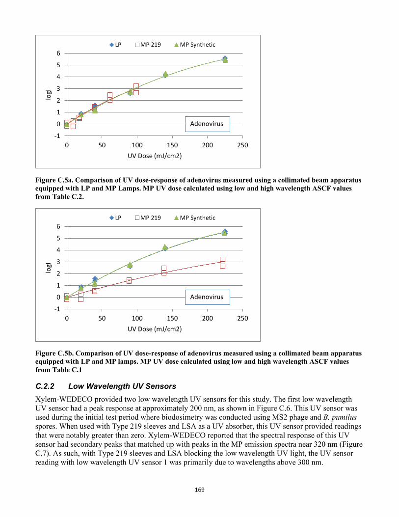
169

-1

0

1

2

3

4

5

6

0 50 100 150 200 250

logI

UV Dose (mJ/cm2)


Adenovirus

Figure C.5a. Comparison of UV dose-response of adenovirus measured using a collimated beam apparatus equipped with LP and MP Lamps. MP UV dose calculated using low and high wavelength ASCF values from Table C.2.

-1

0

1

2

3

4

5

6

0 50 100 150 200 250

logI

UV Dose (mJ/cm2)


Adenovirus

Figure C.5b. Comparison of UV dose-response of adenovirus measured using a collimated beam apparatus equipped with LP and MP lamps. MP UV dose calculated using low and high wavelength ASCF values from Table C.1

C.2.2 Low Wavelength UV SensorsXylem-WEDECO provided two low wavelength UV sensors for this study. The first low wavelength UV sensor had a peak response at approximately 200 nm, as shown in Figure C.6. This UV sensor was used during the initial test period where biodosimetry was conducted using MS2 phage and B. pumilus spores. When used with Type 219 sleeves and LSA as a UV absorber, this UV sensor provided readings that were notably greater than zero. Xylem-WEDECO reported that the spectral response of this UV sensor had secondary peaks that matched up with peaks in the MP emission spectra near 320 nm (Figure C.7). As such, with Type 219 sleeves and LSA blocking the low wavelength UV light, the UV sensorreading with low wavelength UV sensor 1 was primarily due to wavelengths above 300 nm.

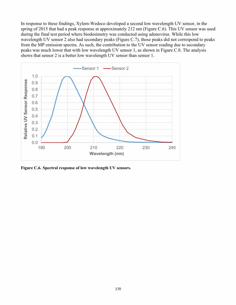
170

In response to these findings, Xylem-Wedeco developed a second low wavelength UV sensor, in the spring of 2015 that had a peak response at approximately 212 nm (Figure C.6). This UV sensor was used during the final test period where biodosimetry was conducted using adenovirus. While this low wavelength UV sensor 2 also had secondary peaks (Figure C.7), those peaks did not correspond to peaks from the MP emission spectra. As such, the contribution to the UV sensor reading due to secondary peaks was much lower that with low wavelength UV sensor 1, as shown in Figure C.8. The analysis shows that sensor 2 is a better low wavelength UV sensor than sensor 1.

0.00.10.20.30.40.50.60.70.80.91.0

190 200 210 220 230 240

Rel

ativ

e U

V Se

nsor

Res

pons

e

Wavelength (nm)

Sensor 1 Sensor 2

Figure C.6. Spectral response of low wavelength UV sensors.

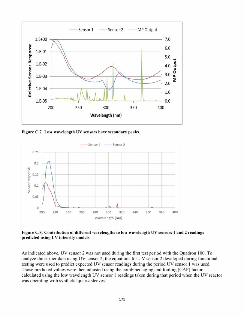
171

0.0

1.0

2.0

3.0

4.0

5.0

6.0

7.0

1.E-05

1.E-04

1.E-03

1.E-02

1.E-01

1.E+00

200 250 300 350 400

MP

Out

put

Rel

etiv

e Se

nsor

Res

pons

e

Wavelength (nm)

Sensor 1 Sensor 2 MP Output

Figure C.7. Low wavelength UV sensors have secondary peaks.

0

0.05

0.1

0.15

0.2

0.25

200 220 240 260 280 300 320 340 360 380 400

Sens

or re

spon

se

Wavelength (nm)

Sensor 1 Sensor 2

Figure C.8. Contribution of different wavelengths to low wavelength UV sensors 1 and 2 readings predicted using UV intensity models.

As indicated above, UV sensor 2 was not used during the first test period with the Quadron 100. To analyze the earlier data using UV sensor 2, the equations for UV sensor 2 developed during functional testing were used to predict expected UV sensor readings during the period UV sensor 1 was used. Those predicted values were then adjusted using the combined aging and fouling (CAF) factor calculated using the low wavelength UV sensor 1 readings taken during that period when the UV reactor was operating with synthetic quartz sleeves.

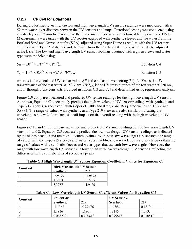
172

C.2.3 UV Sensor EquationsDuring biodosimetric testing, the low and high wavelength UV sensors readings were measured with a 52 mm water layer distance between the UV sensors and lamps. Functional testing was conducted using a water layer of 52 mm to characterize the UV sensor response as a function of lamp power and UVT. Measurements were taken with the UV reactor equipped with synthetic sleeves and the water from the Portland Sand and Gravel Aquifer (SGA) adjusted using Super Hume as well as with the UV reactor equipped with Type 219 sleeves and the water from the Portland Blue Lake Aquifer (BLA) adjusted using LSA. The low and high wavelength UV sensor readings obtained with a given sleeve and water type were modeled using:

𝑆𝑆𝐻𝐻 = 10𝑎𝑎′ × 𝐵𝐵𝑃𝑃𝑏𝑏′ × 𝑈𝑈𝑉𝑉𝑈𝑈254𝑐𝑐′ Equation C.4

𝑆𝑆𝐿𝐿 = 10𝑎𝑎′ × 𝐵𝐵𝑃𝑃𝑏𝑏′ × 𝑡𝑡𝑒𝑒𝑒𝑒(𝑐𝑐′ × 𝑈𝑈𝑉𝑉𝑈𝑈220) Equation C.5

where S is the calculated UV sensor value, BP is the ballast power setting (%), UVT254 is the UV transmittance of the test water at 253.7 nm, UVT220 is the UV transmittance of the test water at 220 nm, and a' through c' are constants provided in Tables C.3 and C.4 and determined using regression analysis.

Figure C.9 compares measured and predicted UV sensor readings for the high wavelength UV sensor. As shown, Equation C.4 accurately predicts the high wavelength UV sensor readings with synthetic and Type 219 sleeves, respectively, with slopes of 1.008 and 0.9977 and R-squared values of 0.9966 and 0.9884. The range of values with synthetic and Type 219 sleeves are also similar, indicating that wavelengths below 240 nm have a small impact on the overall reading with the high wavelength UV sensor.

Figures C.10 and C.11 compare measured and predicted UV sensor readings for the low wavelength UV sensors 1 and 2. Equation C.5 accurately predicts the low wavelength UV sensor readings, as indicated by the slopes near 1.0 and the high R-squared values. With both low wavelength UV sensors, the range of values with the Type 219 sleeves and water types that block low wavelengths are much lower than the range of values with a synthetic sleeves and water types that transmit low wavelengths. However, the range with low wavelength UV sensor 2 is lower than with low wavelength UV sensor 1 reflecting the differences in the contributions of secondary peaks.

Table C.3 High Wavelength UV Sensor Equation Coefficient Values for Equation C.4

Constant High Wavelength UV Sensor Synthetic 219

a -7.9199 -7.0392b 1.3503 1.2755 c 5.3767 4.9426

Table C.4 Low Wavelength UV Sensor Coefficient Values for Equation C.5

Constant UV Sensor 1 UV Sensor 2 Synthetic 219 Synthetic 219

a -1.1362 -0.27476 -1.1362 0.18194 b 1.1926 1.0861 1.2145 1.0533 c 0.065279 0.020813 0.075845 0.010512

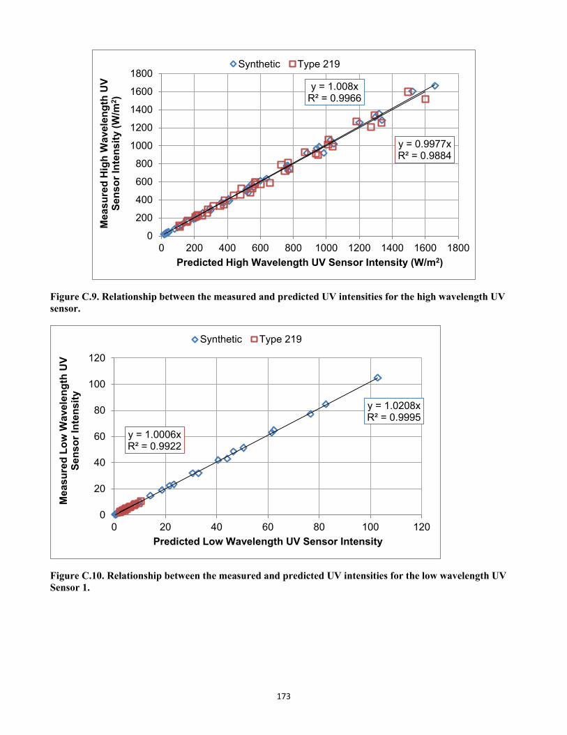
173

y = 1.008xR² = 0.9966

y = 0.9977xR² = 0.9884

0

200

400

600

800

1000

1200

1400

1600

1800

0 200 400 600 800 1000 1200 1400 1600 1800

Mea

sure

d H

igh

Wav

elen

gth

UV

Sens

or In

tens

ity (W

/m2 )

Predicted High Wavelength UV Sensor Intensity (W/m2)

Synthetic Type 219

Figure C.9. Relationship between the measured and predicted UV intensities for the high wavelength UV sensor.

y = 1.0208xR² = 0.9995

y = 1.0006xR² = 0.9922

0

20

40

60

80

100

120

0 20 40 60 80 100 120

Mea

sure

d Lo

w W

avel

engt

h UV

Se

nsor

Inte

nsity

Predicted Low Wavelength UV Sensor Intensity

Synthetic Type 219

Figure C.10. Relationship between the measured and predicted UV intensities for the low wavelength UV Sensor 1.

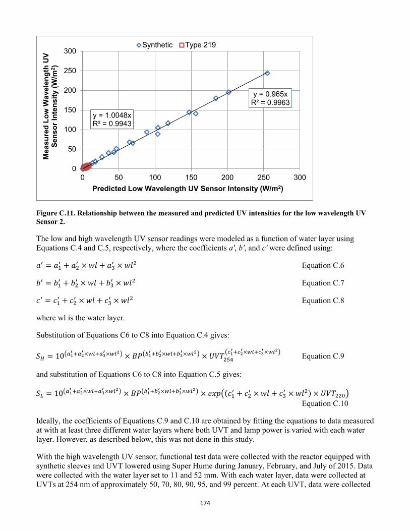
174

y = 0.965xR² = 0.9963

y = 1.0048xR² = 0.9943

0

50

100

150

200

250

300

0 50 100 150 200 250 300

Mea

sure

d Lo

w W

avel

engt

h UV

Sens

or In

tens

ity(W

/m2 )

Predicted Low Wavelength UV Sensor Intensity (W/m2)

Synthetic Type 219

Figure C.11. Relationship between the measured and predicted UV intensities for the low wavelength UV Sensor 2.

The low and high wavelength UV sensor readings were modeled as a function of water layer using Equations C.4 and C.5, respectively, where the coefficients a', b', and c' were defined using:

𝑉𝑉′ = 𝑉𝑉1′ + 𝑉𝑉2′ × 𝑤𝑤𝑉𝑉 + 𝑉𝑉3′ × 𝑤𝑤𝑉𝑉2 Equation C.6

𝑏𝑏′ = 𝑏𝑏1′ + 𝑏𝑏2′ × 𝑤𝑤𝑉𝑉 + 𝑏𝑏3′ × 𝑤𝑤𝑉𝑉2 Equation C.7

𝑐𝑐′ = 𝑐𝑐1′ + 𝑐𝑐2′ × 𝑤𝑤𝑉𝑉 + 𝑐𝑐3′ × 𝑤𝑤𝑉𝑉2 Equation C.8

where wl is the water layer.

Substitution of Equations C6 to C8 into Equation C.4 gives:

𝑆𝑆𝐻𝐻 = 10�𝑎𝑎1′+𝑎𝑎2′×𝐿𝐿𝑃𝑃+𝑎𝑎3′×𝐿𝐿𝑃𝑃2� × 𝐵𝐵𝑃𝑃�𝑏𝑏1′+𝑏𝑏2′×𝐿𝐿𝑃𝑃+𝑏𝑏3′×𝐿𝐿𝑃𝑃2� × 𝑈𝑈𝑉𝑉𝑈𝑈254�𝑐𝑐1′+𝑐𝑐2′×𝐿𝐿𝑃𝑃+𝑐𝑐3′×𝐿𝐿𝑃𝑃2� Equation C.9

and substitution of Equations C6 to C8 into Equation C.5 gives:

𝑆𝑆𝐿𝐿 = 10�𝑎𝑎1′+𝑎𝑎2′×𝐿𝐿𝑃𝑃+𝑎𝑎3′×𝐿𝐿𝑃𝑃2� × 𝐵𝐵𝑃𝑃�𝑏𝑏1′+𝑏𝑏2′×𝐿𝐿𝑃𝑃+𝑏𝑏3′×𝐿𝐿𝑃𝑃2� × 𝑡𝑡𝑒𝑒𝑒𝑒�(𝑐𝑐1′ + 𝑐𝑐2′ × 𝑤𝑤𝑉𝑉 + 𝑐𝑐3′ × 𝑤𝑤𝑉𝑉2) × 𝑈𝑈𝑉𝑉𝑈𝑈220�Equation C.10

Ideally, the coefficients of Equations C.9 and C.10 are obtained by fitting the equations to data measured at with at least three different water layers where both UVT and lamp power is varied with each water layer. However, as described below, this was not done in this study.

With the high wavelength UV sensor, functional test data were collected with the reactor equipped with synthetic sleeves and UVT lowered using Super Hume during January, February, and July of 2015. Data were collected with the water layer set to 11 and 52 mm. With each water layer, data were collected at UVTs at 254 nm of approximately 50, 70, 80, 90, 95, and 99 percent. At each UVT, data were collected

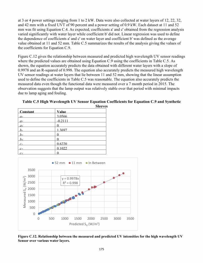
175

at 3 or 4 power settings ranging from 1 to 2 kW. Data were also collected at water layers of 12, 22, 32, and 42 mm with a fixed UVT of 90 percent and a power setting of 0.9 kW. Each dataset at 11 and 52 mm was fit using Equation C.4. As expected, coefficients a' and c' obtained from the regression analysis varied significantly with water layer while coefficient b' did not. Linear regression was used to define the dependence of coefficients a' and c' on water layer and coefficient b' was defined as the average value obtained at 11 and 52 mm. Table C.5 summarizes the results of the analysis giving the values of the coefficients for Equation C.9.

Figure C.12 gives the relationship between measured and predicted high wavelength UV sensor readings where the predicted values are obtained using Equation C.9 using the coefficients in Table C.5. As shown, the equation accurately predicts the data obtained with different water layers with a slope of 0.9978 and an R-squared of 0.998. The equation also accurately predicts the measured high wavelength UV sensor readings at water layers that lie between 11 and 52 mm, showing that the linear assumption used to define the coefficients in Table C.5 was reasonable. The equation also accurately predicts the measured data even though the functional data were measured over a 7 month period in 2015. The observation suggests that the lamp output was relatively stable over that period with minimal impacts due to lamp aging and fouling.

Table C.5 High Wavelength UV Sensor Equation Coefficients for Equation C.9 and Synthetic Sleeves

Constant Valuea1 3.0566a2 -0.2111a3 0b1 1.3697b2 0b3 0c1 0.6220c2 0.1022c3 0

Figure C.12. Relationship between the measured and predicted UV intensities for the high wavelength UV Sensor over various water layers.

y = 0.9978xR² = 0.998

0

500

1000

1500

2000

2500

3000

3500

0 500 1000 1500 2000 2500 3000 3500

Mer

asur

ed S

H(W

/m2 )

Predicted SH (W/m2)

52 mm 11 mm In Between

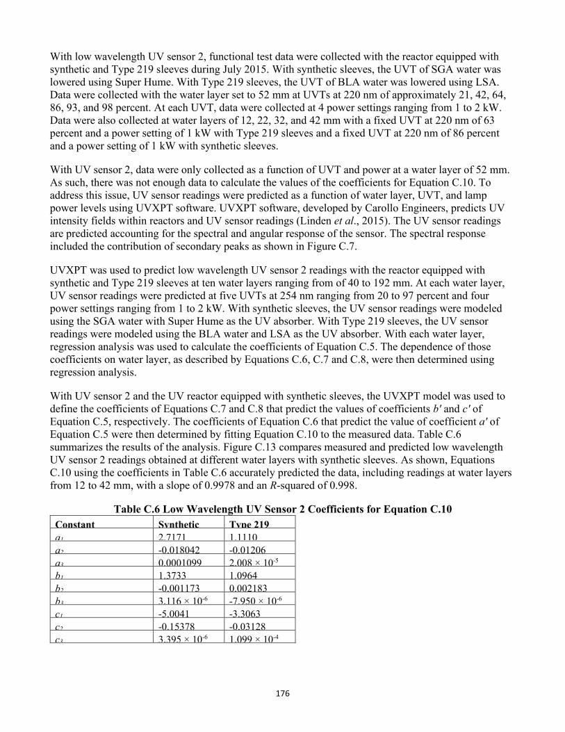
176

With low wavelength UV sensor 2, functional test data were collected with the reactor equipped with synthetic and Type 219 sleeves during July 2015. With synthetic sleeves, the UVT of SGA water was lowered using Super Hume. With Type 219 sleeves, the UVT of BLA water was lowered using LSA. Data were collected with the water layer set to 52 mm at UVTs at 220 nm of approximately 21, 42, 64, 86, 93, and 98 percent. At each UVT, data were collected at 4 power settings ranging from 1 to 2 kW. Data were also collected at water layers of 12, 22, 32, and 42 mm with a fixed UVT at 220 nm of 63 percent and a power setting of 1 kW with Type 219 sleeves and a fixed UVT at 220 nm of 86 percent and a power setting of 1 kW with synthetic sleeves.

With UV sensor 2, data were only collected as a function of UVT and power at a water layer of 52 mm. As such, there was not enough data to calculate the values of the coefficients for Equation C.10. To address this issue, UV sensor readings were predicted as a function of water layer, UVT, and lamp power levels using UVXPT software. UVXPT software, developed by Carollo Engineers, predicts UV intensity fields within reactors and UV sensor readings (Linden et al., 2015). The UV sensor readings are predicted accounting for the spectral and angular response of the sensor. The spectral response included the contribution of secondary peaks as shown in Figure C.7.

UVXPT was used to predict low wavelength UV sensor 2 readings with the reactor equipped with synthetic and Type 219 sleeves at ten water layers ranging from of 40 to 192 mm. At each water layer, UV sensor readings were predicted at five UVTs at 254 nm ranging from 20 to 97 percent and four power settings ranging from 1 to 2 kW. With synthetic sleeves, the UV sensor readings were modeled using the SGA water with Super Hume as the UV absorber. With Type 219 sleeves, the UV sensor readings were modeled using the BLA water and LSA as the UV absorber. With each water layer, regression analysis was used to calculate the coefficients of Equation C.5. The dependence of those coefficients on water layer, as described by Equations C.6, C.7 and C.8, were then determined using regression analysis.

With UV sensor 2 and the UV reactor equipped with synthetic sleeves, the UVXPT model was used to define the coefficients of Equations C.7 and C.8 that predict the values of coefficients b' and c' of Equation C.5, respectively. The coefficients of Equation C.6 that predict the value of coefficient a' of Equation C.5 were then determined by fitting Equation C.10 to the measured data. Table C.6 summarizes the results of the analysis. Figure C.13 compares measured and predicted low wavelength UV sensor 2 readings obtained at different water layers with synthetic sleeves. As shown, Equations C.10 using the coefficients in Table C.6 accurately predicted the data, including readings at water layers from 12 to 42 mm, with a slope of 0.9978 and an R-squared of 0.998.

Table C.6 Low Wavelength UV Sensor 2 Coefficients for Equation C.10 Constant Synthetic Type 219 a1 2.7171 1.1110 a2 -0.018042 -0.01206 a3 0.0001099 2.008 × 10-5 b1 1.3733 1.0964 b2 -0.001173 0.002183 b3 3.116 × 10-6 -7.950 × 10-6 c1 -5.0041 -3.3063 c2 -0.15378 -0.03128 c3 3.395 × 10-6 1.099 × 10-4

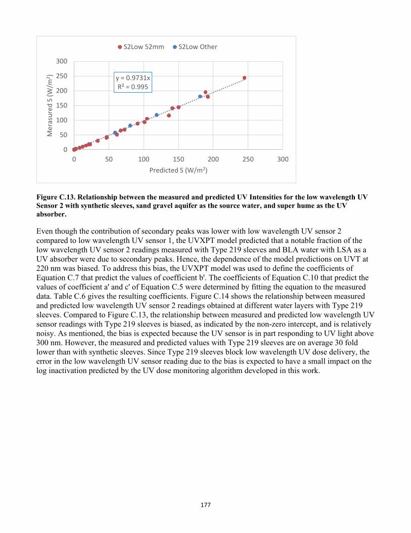
177

y = 0.9731xR² = 0.995

0

50

100

150

200

250

300

0 50 100 150 200 250 300

Mer

asur

ed S

(W/m

2 )

Predicted S (W/m2)

S2Low 52mm S2Low Other

Figure C.13. Relationship between the measured and predicted UV Intensities for the low wavelength UV Sensor 2 with synthetic sleeves, sand gravel aquifer as the source water, and super hume as the UV absorber.

Even though the contribution of secondary peaks was lower with low wavelength UV sensor 2 compared to low wavelength UV sensor 1, the UVXPT model predicted that a notable fraction of the low wavelength UV sensor 2 readings measured with Type 219 sleeves and BLA water with LSA as a UV absorber were due to secondary peaks. Hence, the dependence of the model predictions on UVT at 220 nm was biased. To address this bias, the UVXPT model was used to define the coefficients of Equation C.7 that predict the values of coefficient b'. The coefficients of Equation C.10 that predict the values of coefficient a' and c' of Equation C.5 were determined by fitting the equation to the measured data. Table C.6 gives the resulting coefficients. Figure C.14 shows the relationship between measured and predicted low wavelength UV sensor 2 readings obtained at different water layers with Type 219 sleeves. Compared to Figure C.13, the relationship between measured and predicted low wavelength UV sensor readings with Type 219 sleeves is biased, as indicated by the non-zero intercept, and is relatively noisy. As mentioned, the bias is expected because the UV sensor is in part responding to UV light above 300 nm. However, the measured and predicted values with Type 219 sleeves are on average 30 fold lower than with synthetic sleeves. Since Type 219 sleeves block low wavelength UV dose delivery, the error in the low wavelength UV sensor reading due to the bias is expected to have a small impact on the log inactivation predicted by the UV dose monitoring algorithm developed in this work.

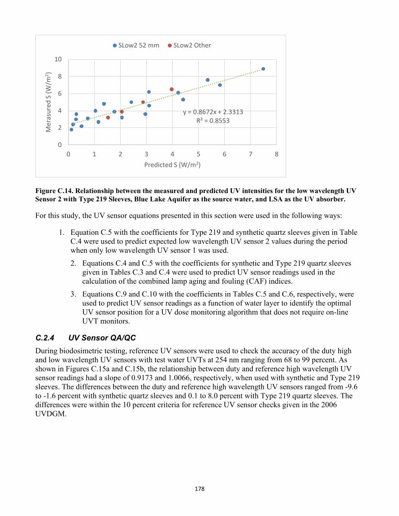
178

y = 0.8672x + 2.3313R² = 0.8553

0

2

4

6

8

10

0 1 2 3 4 5 6 7 8

Mer

asur

ed S

(W/m

2 )

Predicted S (W/m2)

SLow2 52 mm SLow2 Other

Figure C.14. Relationship between the measured and predicted UV intensities for the low wavelength UV Sensor 2 with Type 219 Sleeves, Blue Lake Aquifer as the source water, and LSA as the UV absorber.

For this study, the UV sensor equations presented in this section were used in the following ways:

1. Equation C.5 with the coefficients for Type 219 and synthetic quartz sleeves given in Table C.4 were used to predict expected low wavelength UV sensor 2 values during the period when only low wavelength UV sensor 1 was used. 2. Equations C.4 and C.5 with the coefficients for synthetic and Type 219 quartz sleeves

given in Tables C.3 and C.4 were used to predict UV sensor readings used in the calculation of the combined lamp aging and fouling (CAF) indices.

3. Equations C.9 and C.10 with the coefficients in Tables C.5 and C.6, respectively, were used to predict UV sensor readings as a function of water layer to identify the optimal UV sensor position for a UV dose monitoring algorithm that does not require on-line UVT monitors.

C.2.4 UV Sensor QA/QC During biodosimetric testing, reference UV sensors were used to check the accuracy of the duty high and low wavelength UV sensors with test water UVTs at 254 nm ranging from 68 to 99 percent. As shown in Figures C.15a and C.15b, the relationship between duty and reference high wavelength UV sensor readings had a slope of 0.9173 and 1.0066, respectively, when used with synthetic and Type 219 sleeves. The differences between the duty and reference high wavelength UV sensors ranged from -9.6 to -1.6 percent with synthetic quartz sleeves and 0.1 to 8.0 percent with Type 219 quartz sleeves. The differences were within the 10 percent criteria for reference UV sensor checks given in the 2006 UVDGM.

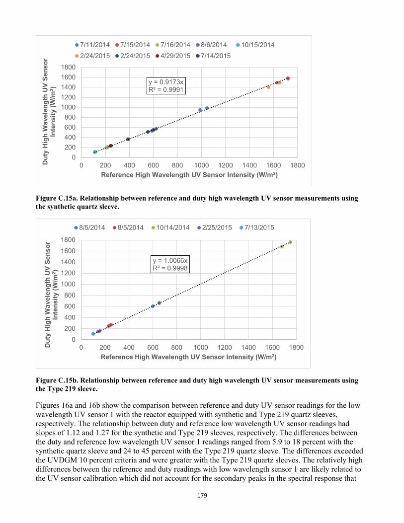
179

y = 0.9173xR² = 0.9991

0200400600800

10001200140016001800

0 200 400 600 800 1000 1200 1400 1600 1800Dut

y H

igh

Wav

elen

gth

UV

Sens

or

Inte

nsity

(W/m

2 )

Reference High Wavelength UV Sensor Intensity (W/m2)

7/11/2014 7/15/2014 7/16/2014 8/6/2014 10/15/20142/24/2015 2/24/2015 4/29/2015 7/14/2015

Figure C.15a. Relationship between reference and duty high wavelength UV sensor measurements using the synthetic quartz sleeve.

y = 1.0066xR² = 0.9998

0200400600800

10001200140016001800

0 200 400 600 800 1000 1200 1400 1600 1800Dut

y H

igh

Wav

elen

gth

UV

Sens

or

Inte

nsity

(W/m

2 )

Reference High Wavelength UV Sensor Intensity (W/m2)

8/5/2014 8/5/2014 10/14/2014 2/25/2015 7/13/2015

Figure C.15b. Relationship between reference and duty high wavelength UV sensor measurements using the Type 219 sleeve.

Figures 16a and 16b show the comparison between reference and duty UV sensor readings for the low wavelength UV sensor 1 with the reactor equipped with synthetic and Type 219 quartz sleeves, respectively. The relationship between duty and reference low wavelength UV sensor readings had slopes of 1.12 and 1.27 for the synthetic and Type 219 sleeves, respectively. The differences between the duty and reference low wavelength UV sensor 1 readings ranged from 5.9 to 18 percent with the synthetic quartz sleeve and 24 to 45 percent with the Type 219 quartz sleeve. The differences exceeded the UVDGM 10 percent criteria and were greater with the Type 219 quartz sleeves. The relatively high differences between the reference and duty readings with low wavelength sensor 1 are likely related to the UV sensor calibration which did not account for the secondary peaks in the spectral response that

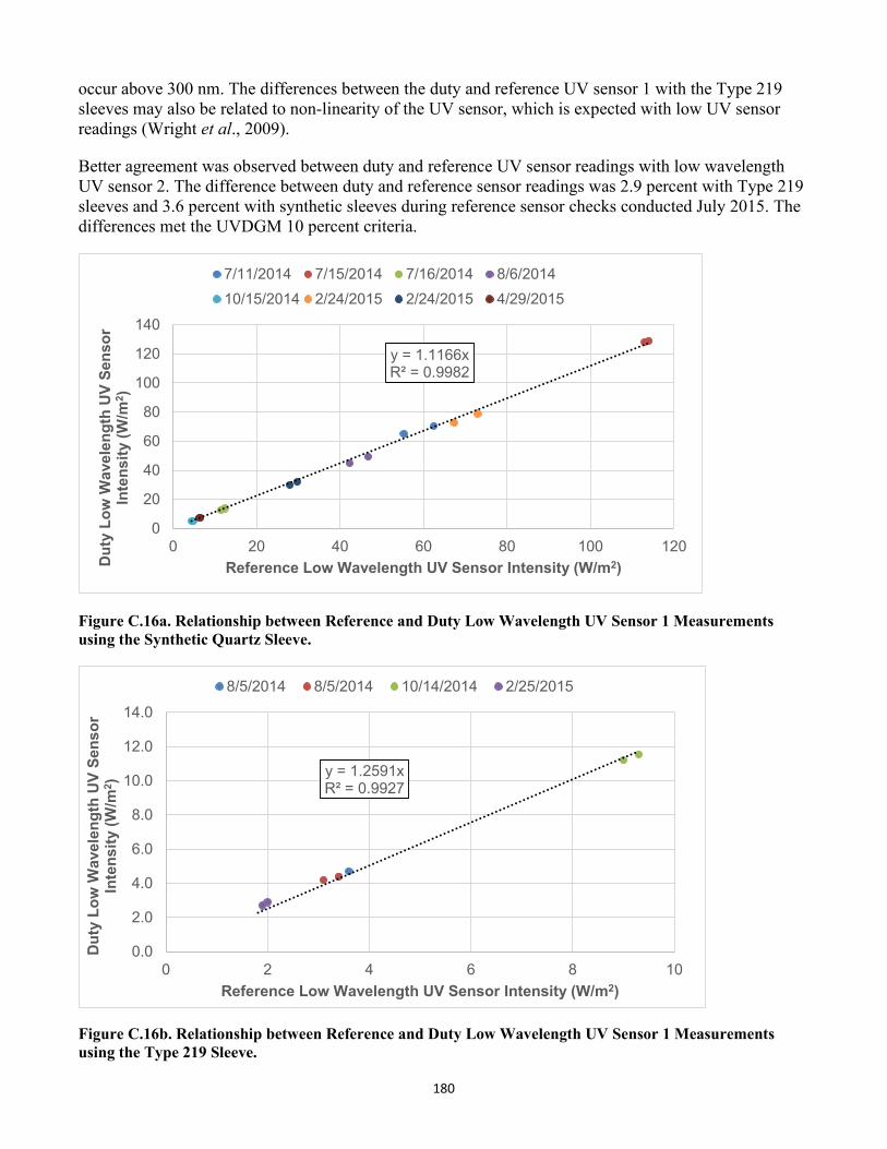
180

occur above 300 nm. The differences between the duty and reference UV sensor 1 with the Type 219 sleeves may also be related to non-linearity of the UV sensor, which is expected with low UV sensor readings (Wright et al., 2009).

Better agreement was observed between duty and reference UV sensor readings with low wavelength UV sensor 2. The difference between duty and reference sensor readings was 2.9 percent with Type 219 sleeves and 3.6 percent with synthetic sleeves during reference sensor checks conducted July 2015. The differences met the UVDGM 10 percent criteria.

y = 1.1166xR² = 0.9982

0

20

40

60

80

100

120

140

0 20 40 60 80 100 120

Dut

y Lo

w W

avel

engt

h U

V Se

nsor

In

tens

ity (W

/m2 )

Reference Low Wavelength UV Sensor Intensity (W/m2)

7/11/2014 7/15/2014 7/16/2014 8/6/201410/15/2014 2/24/2015 2/24/2015 4/29/2015

Figure C.16a. Relationship between Reference and Duty Low Wavelength UV Sensor 1 Measurements using the Synthetic Quartz Sleeve.

y = 1.2591xR² = 0.9927

0.0

2.0

4.0

6.0

8.0

10.0

12.0

14.0

0 2 4 6 8 10

Dut

y Lo

w W

avel

engt

h U

V Se

nsor

In

tens

ity (W

/m2 )

Reference Low Wavelength UV Sensor Intensity (W/m2)

8/5/2014 8/5/2014 10/14/2014 2/25/2015

Figure C.16b. Relationship between Reference and Duty Low Wavelength UV Sensor 1 Measurements using the Type 219 Sleeve.

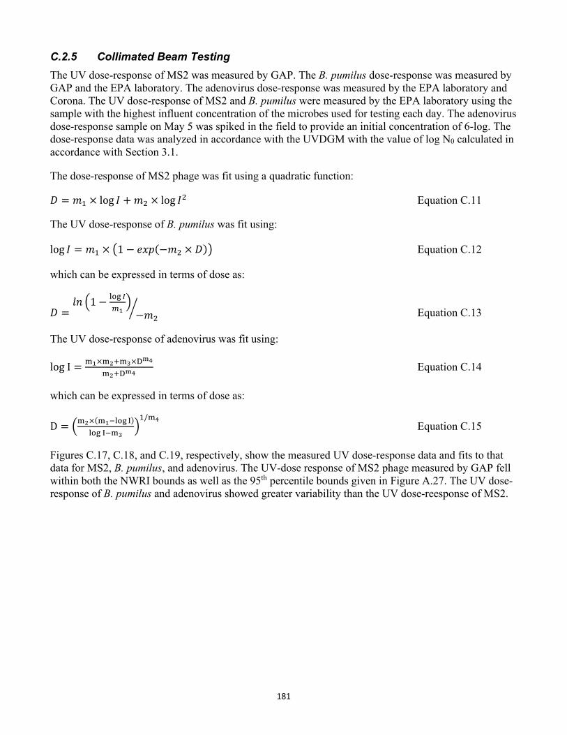
181

C.2.5 Collimated Beam Testing The UV dose-response of MS2 was measured by GAP. The B. pumilus dose-response was measured by GAP and the EPA laboratory. The adenovirus dose-response was measured by the EPA laboratory and Corona. The UV dose-response of MS2 and B. pumilus were measured by the EPA laboratory using the sample with the highest influent concentration of the microbes used for testing each day. The adenovirus dose-response sample on May 5 was spiked in the field to provide an initial concentration of 6-log. The dose-response data was analyzed in accordance with the UVDGM with the value of log N0 calculated in accordance with Section 3.1.

The dose-response of MS2 phage was fit using a quadratic function:

𝐷𝐷 = 𝑚𝑚1 × log 𝐼𝐼 + 𝑚𝑚2 × log 𝐼𝐼2 Equation C.11

The UV dose-response of B. pumilus was fit using:

log 𝐼𝐼 = 𝑚𝑚1 × �1 − 𝑡𝑡𝑒𝑒𝑒𝑒(−𝑚𝑚2 × 𝐷𝐷)� Equation C.12


𝐷𝐷 =𝑉𝑉𝑆𝑆 �1 − log 𝐼𝐼

𝑛𝑛1�−𝑚𝑚2� Equation C.13

The UV dose-response of adenovirus was fit using:

log I = m1×m2+m3×Dm4

m2+Dm4 Equation C.14


D = �m2×(m1−log I)log I−m3

�1/m4

Equation C.15

Figures C.17, C.18, and C.19, respectively, show the measured UV dose-response data and fits to that data for MS2, B. pumilus, and adenovirus. The UV-dose response of MS2 phage measured by GAP fell within both the NWRI bounds as well as the 95th percentile bounds given in Figure A.27. The UV dose-response of B. pumilus and adenovirus showed greater variability than the UV dose-reesponse of MS2.

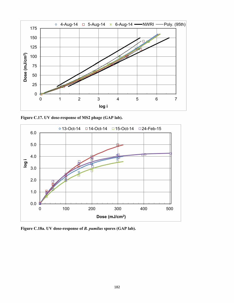
182

0

25

50

75

100

125

150

175

0 1 2 3 4 5 6 7

Dose

(mJ/

cm2 )

log i

4-Aug-14 5-Aug-14 6-Aug-14 NWRI Poly. (95th)

Figure C.17. UV dose-response of MS2 phage (GAP lab).

0.0

1.0

2.0

3.0

4.0

5.0

6.0

0 100 200 300 400 500

log

i

Dose (mJ/cm2)

13-Oct-14 14-Oct-14 15-Oct-14 24-Feb-15

Figure C.18a. UV dose-response of B. pumilus spores (GAP lab).

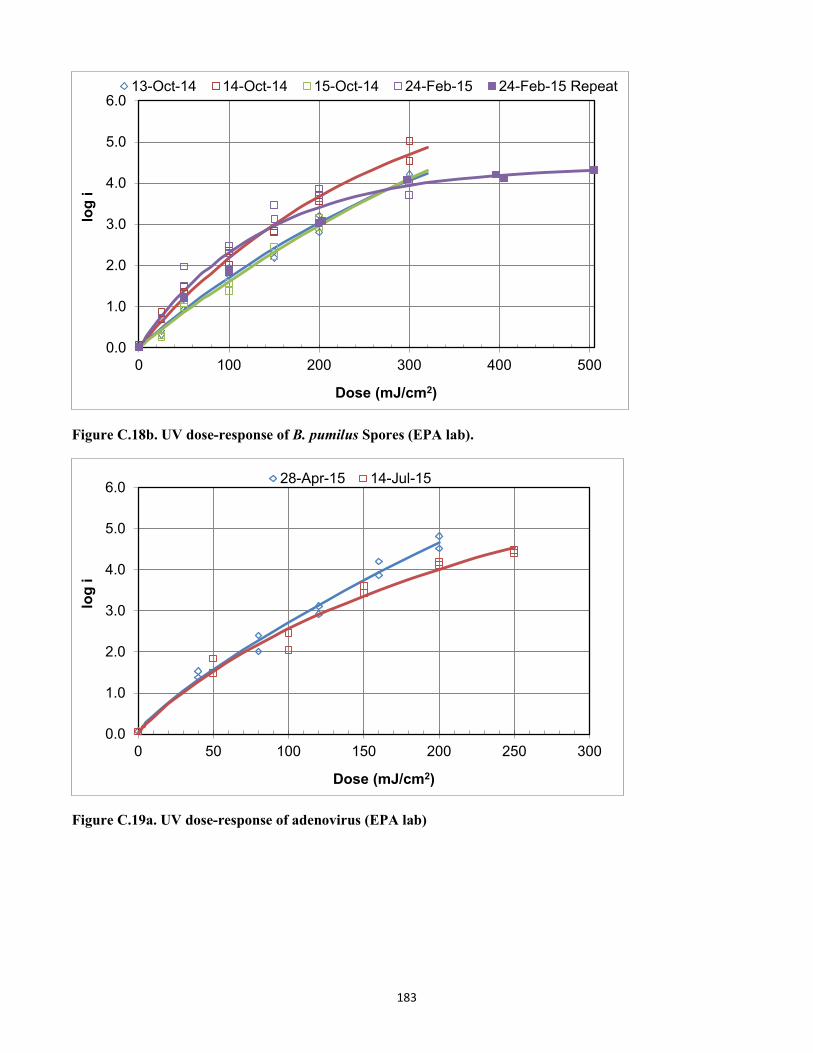
183

0.0

1.0

2.0

3.0

4.0

5.0

6.0

0 100 200 300 400 500

log

i

Dose (mJ/cm2)

13-Oct-14 14-Oct-14 15-Oct-14 24-Feb-15 24-Feb-15 Repeat

Figure C.18b. UV dose-response of B. pumilus Spores (EPA lab).

0.0

1.0

2.0

3.0

4.0

5.0

6.0

0 50 100 150 200 250 300

log

i

Dose (mJ/cm2)

28-Apr-15 14-Jul-15

Figure C.19a. UV dose-response of adenovirus (EPA lab)

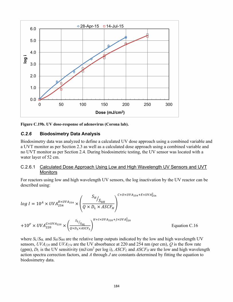
184

0.0

1.0

2.0

3.0

4.0

5.0

6.0

0 50 100 150 200 250 300

log

i

Dose (mJ/cm2)

28-Apr-15 14-Jul-15

Figure C.19b. UV dose-response of adenovirus (Corona lab).

C.2.6 Biodosimetry Data Analysis Biodosimetry data was analyzed to define a calculated UV dose approach using a combined variable and a UVT monitor as per Section 2.3 as well as a calculated dose approach using a combined variable and no UVT monitor as per Section 2.4. During biodosimetric testing, the UV sensor was located with a water layer of 52 cm.

C.2.6.1 Calculated Dose Approach Using Low and High Wavelength UV Sensors and UVT Monitors

For reactors using low and high wavelength UV sensors, the log inactivation by the UV reactor can be described using:








Equation C.16

where SL/S0L and SH/S0H are the relative lamp outputs indicated by the low and high wavelength UV sensors, UVA220 and UVA254 are the UV absorbance at 220 and 254 nm (per cm), Q is the flow rate (gpm), DL is the UV sensitivity (mJ/cm2 per log i), ASCFL and ASCFH are the low and high wavelength action spectra correction factors, and A through J are constants determined by fitting the equation to biodosimetry data.

185

Equation C.16 was fit to the biodosimetry data using the following steps:

1. Calculate the average flow measured over the duration of each test condition. 2. Calculate the average UVT220 and UVT254 measured over the duration of each test

condition. Typically, one UVT sample was analyzed with each influent and effluent grab sample used to measure log inactivation. Calculate the average UVA220 and average UVA254 using the average UVT values.

3. With each test condition, calculate the average high wavelength UV sensor value, SH, using the measured data.

4. With each test condition done using low wavelength UV sensor 1, calculate the average low wavelength UV sensor 1 value, SL, using the measured data.

5. With each test condition done using low wavelength UV sensor 2, calculate the average low wavelength UV sensor 2 value, SL, using the measured data.

6. With each test condition, use Equation C.4 with the coefficients in Table C.3 to predict the high wavelength UV sensor readings.

7. With each test condition, use Equation C.5 with the coefficients in Table C.4 to predict the low wavelength UV sensor readings for UV sensors 1 and 2.

8. With each test condition and UV sensor used, calculate the CAF index as the ratio of the average measured UV sensor value (step 3, 4 or 5) divided by the predicted value (step 6 or 7).

9. With each test condition where UV sensor 2 was not used, adjust the UV sensor 2 value from Step 7 by the average CAF index for that day of testing calculated for UV sensor 1 when used with the reactor operating with synthetic sleeves. With synthetic sleeves, low wavelength UV sensor 1 acts primarily as a low wavelength sensor with minimal impact from spectral response above 300 nm. The results of this step are predicted UV sensor 2 values adjusted for lamp aging and fouling. An underlying assumption of this approach is that the lamp aging and fouling at low wavelengths has a similar impact on both UV sensor 1 and 2.

10. With each test condition, calculate the value of S0 for the high wavelength UV sensor using Equation C.4 and the synthetic sleeve coefficients given in Table C.3. For this calculation, PL in Equation C.4 was set to 100 percent ballast power and UVT254 was set to the average UVT254 determined in Step 2.

11. With each test condition, calculate the value of S0 for low wavelength UV sensor 2 using Equation C.5 and the coefficients for the synthetic sleeve given in Table C.4. For this calculation, PL in Equation C.5 was set to 100 percent ballast power and UVT220 was set to the average UVT220 determined in Step 2.

12. With each test condition, calculate the relative lamp output, S/S0, for the high wavelength UV sensor using average measured UV sensor readings from Step 3 and the S0 values calculated in Step 10.

13. With each test condition, calculate the relative lamp output, S/S0, for low wavelength UV sensor 2 using the predicted values from Step 9 and the S0 values calculated in Step 11.

14. With each influent sample, calculate the average of the replicate plate counts (Ni) and take its log transformation.

186

15. With each effluent sample, calculate the average of the replicate plate counts (Ne) and take its log transformation. If any replicate had zero plate counts, calculate the log transform of the average of the plate counts with all replicates. If all replicates had zero plate counts, discard the data.

16. With each test condition, calculate the log inactivation of each replicate pair of inlet and outlet samples using:

𝑉𝑉𝐷𝐷𝑙𝑙 𝐼𝐼 = 𝑉𝑉𝐷𝐷𝑙𝑙 𝑁𝑁𝑀𝑀 − 𝑉𝑉𝐷𝐷𝑙𝑙 𝑁𝑁𝑒𝑒Equation C.17

where log Ni and log Ne are the influent and effluent log concentrations calculated, respectively, from Steps 14 and 15.

17. Remove any test conditions where the measured log inactivation is greater than the maximum log inactivation used to define the test microbe UV dose-response curve or where the number of plate counts is one or less.

18. Calculate the reduction equivalent dose (RED) associated with each log inactivation using the UV dose-response of the test microbe measured on the same day of the test condition (i.e., use Equation C.11, C.13, or C.15).

19. With each test condition replicate, calculate the value of DL as the RED from Step 18 divided by the log inactivation from Step 16.

20. Using multivariate linear regression, fit the MS2 data measured with Type 219 sleeves to:

𝑉𝑉𝐷𝐷𝑙𝑙(log 𝐼𝐼𝐻𝐻) = 𝐴𝐴 + 𝐵𝐵 × 𝑈𝑈𝑉𝑉𝐴𝐴254 × 𝑉𝑉𝐷𝐷𝑙𝑙(𝑈𝑈𝑉𝑉𝐴𝐴254) + �𝐴𝐴 + 𝐷𝐷 × 𝑈𝑈𝑉𝑉𝐴𝐴254 + 𝑅𝑅 × 𝑈𝑈𝑉𝑉𝐴𝐴2542� ×

𝑉𝑉𝐷𝐷𝑙𝑙 �𝑆𝑆𝐻𝐻


𝑄𝑄×𝑅𝑅𝐿𝐿×𝐴𝐴𝑆𝑆𝐶𝐶𝐹𝐹𝐻𝐻�Equation C.18a

The linear regression did not include the controls. The results from this linear regression provided initial estimates for the coefficients A through E.

21. With the MS2 data measured with synthetric sleeves, calculate the difference in the measured log inactivation and the log inactivation predicted using Equation C.18a.

22. Using multivariate linear regression,fit the difference from Step 21 to:

𝑉𝑉𝐷𝐷𝑙𝑙(log 𝐼𝐼𝐿𝐿) = 𝑉𝑉 + 𝐺𝐺 × 𝑈𝑈𝑉𝑉𝐴𝐴220 × 𝑉𝑉𝐷𝐷𝑙𝑙(𝑈𝑈𝑉𝑉𝐴𝐴220) + �𝐻𝐻 + 𝐼𝐼 × 𝑈𝑈𝑉𝑉𝐴𝐴220 + 𝐽𝐽 × 𝑈𝑈𝑉𝑉𝐴𝐴2202� ×

𝑉𝑉𝐷𝐷𝑙𝑙 �𝑆𝑆𝐿𝐿


𝑄𝑄×𝑅𝑅𝐿𝐿×𝐴𝐴𝑆𝑆𝐶𝐶𝐹𝐹𝐿𝐿�Equation C.18b

The linear regression did not include the controls. The results from this linear regression provided initial estimates for the coefficients F through J.

23. If any coefficient has a p-statistic greater than 0.05, remove the coefficient with the highest value of the p-statistic and repeat steps 20 and 22 until all coefficients are statistically significant.

24. Using non-linear multivariate regression, fit the biodosimetry data (including controls) to Equation C.16. The non-linear multivariate regression uses the results from Steps 20 and 22 as initial values for the equation coefficients and is run to minimize the sum of the squares of the residuals defined as the difference between the predicted and measured log inactivation. The high wavelength coefficients A to E are solved first by minimizing the sum of the squares of the residuals of the Type 219 data. Then the low wavelength coefficients F to J are

187

solved by minimizing the sum of the squares of the synthetic data holding the values of coefficients A to E constant. Finally, the model is fine-tuned by solving for all the coefficients.

25. In this step, the UV sensitivity is defined as:

𝐷𝐷𝐿𝐿 = 𝐷𝐷𝑉𝑉𝐷𝐷𝑙𝑙 � 𝐼𝐼Equation C.19

where log I is the predicted log I obtained using Equation C.16 and RED is the UV dose determined using Equation C.11. Since the value of DL depends on the predicted log I, the analysis iteratively determined the predicted value of log I and DL. The iteration used a starting log I value of 3.0, which was used to calculate a starting value of DL. The next value of log I was then determined using Equation C.16, the result of which was used to determine the next value of DL. The iteration was repeated nine times resulting in an absolute difference between log IN+1 and log IN was less than 0.001.

26. Calculate the standard deviation of the differences between the measured and predicted log inactivations.

27. Calculate a Grubbs statistic (NIST/SEMATECH, 2012) for the number of test conditions and for the total number of replicates using:

𝐺𝐺 = 𝐼𝐼−1√𝐼𝐼

× �𝑡𝑡� 𝑝𝑝2×𝑙𝑙,𝐼𝐼−2�

2

𝐼𝐼−2+𝑡𝑡� 𝑝𝑝2×𝑙𝑙,𝐼𝐼−2�

2Equation C.20

where N is the number of data points used to define the fitted equation, t is a Student’s t-statistic with N-2 degrees of freedom, and p is the probability of the outlier. In this analysis, p was set to 0.1.

28. Identify data outliers as values with a residual greater than the product of the Grubbs statistic and the standard deviation of the residuals. Remove the worst outlier and repeat steps 20 to 24 until no outliers are identified. The initial analysis fitted Equation C.16 to the MS2 data and used the resulting equation to predict the log inactivation of B. pumilus and adenovirus. The second analysis used the UVA at 230 nm instead of the UVA at 220 nm. The third analysis fitted Equation C.16 to the combined MS2 and B. pumilus data and used the resulting equation to predict the log inactivation of adenovirus. With MS2 and B. pumilus, Equation C.16 used the low and high ASCF values given in Table C.2. With adenovirus, Equation C.16 used the low and high ASCF values given in Table C.1.

Table C.7 summarizes the number of test conditions with each challenge microorganism and the number removed from the analysis because the log inactivation exceeded the maximum with the UV dose response, because the plates had zero counts, or because of a lab error. Two MS2 replicates were removed when Equation C.16 was fit to the MS2 data but none were removed as outliers when the equation was fit to the combined data set of MS2 and EPA or GAP B. pumilus.

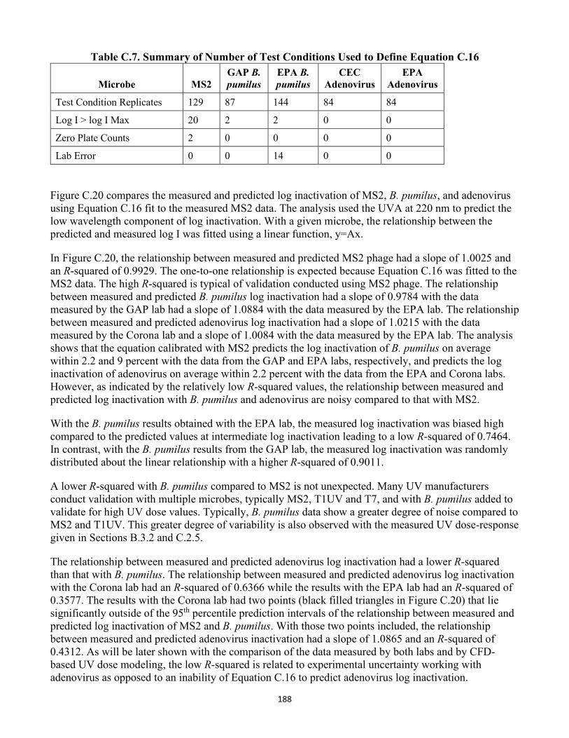
188

Table C.7. Summary of Number of Test Conditions Used to Define Equation C.16

Microbe MS2 GAP B. pumilus

EPA B. pumilus

CEC Adenovirus

EPA Adenovirus

Test Condition Replicates 129 87 144 84 84

Log I > log I Max 20 2 2 0 0

Zero Plate Counts 2 0 0 0 0

Lab Error 0 0 14 0 0

Figure C.20 compares the measured and predicted log inactivation of MS2, B. pumilus, and adenovirus using Equation C.16 fit to the measured MS2 data. The analysis used the UVA at 220 nm to predict the low wavelength component of log inactivation. With a given microbe, the relationship between the predicted and measured log I was fitted using a linear function, y=Ax.

In Figure C.20, the relationship between measured and predicted MS2 phage had a slope of 1.0025 and an R-squared of 0.9929. The one-to-one relationship is expected because Equation C.16 was fitted to the MS2 data. The high R-squared is typical of validation conducted using MS2 phage. The relationship between measured and predicted B. pumilus log inactivation had a slope of 0.9784 with the data measured by the GAP lab had a slope of 1.0884 with the data measured by the EPA lab. The relationship between measured and predicted adenovirus log inactivation had a slope of 1.0215 with the data measured by the Corona lab and a slope of 1.0084 with the data measured by the EPA lab. The analysis shows that the equation calibrated with MS2 predicts the log inactivation of B. pumilus on average within 2.2 and 9 percent with the data from the GAP and EPA labs, respectively, and predicts the log inactivation of adenovirus on average within 2.2 percent with the data from the EPA and Corona labs. However, as indicated by the relatively low R-squared values, the relationship between measured and predicted log inactivation with B. pumilus and adenovirus are noisy compared to that with MS2.

With the B. pumilus results obtained with the EPA lab, the measured log inactivation was biased high compared to the predicted values at intermediate log inactivation leading to a low R-squared of 0.7464. In contrast, with the B. pumilus results from the GAP lab, the measured log inactivation was randomly distributed about the linear relationship with a higher R-squared of 0.9011.

A lower R-squared with B. pumilus compared to MS2 is not unexpected. Many UV manufacturers conduct validation with multiple microbes, typically MS2, T1UV and T7, and with B. pumilus added to validate for high UV dose values. Typically, B. pumilus data show a greater degree of noise compared to MS2 and T1UV. This greater degree of variability is also observed with the measured UV dose-response given in Sections B.3.2 and C.2.5.

The relationship between measured and predicted adenovirus log inactivation had a lower R-squared than that with B. pumilus. The relationship between measured and predicted adenovirus log inactivation with the Corona lab had an R-squared of 0.6366 while the results with the EPA lab had an R-squared of 0.3577. The results with the Corona lab had two points (black filled triangles in Figure C.20) that lie significantly outside of the 95th percentile prediction intervals of the relationship between measured and predicted log inactivation of MS2 and B. pumilus. With those two points included, the relationship between measured and predicted adenovirus inactivation had a slope of 1.0865 and an R-squared of 0.4312. As will be later shown with the comparison of the data measured by both labs and by CFD-based UV dose modeling, the low R-squared is related to experimental uncertainty working with adenovirus as opposed to an inability of Equation C.16 to predict adenovirus log inactivation.

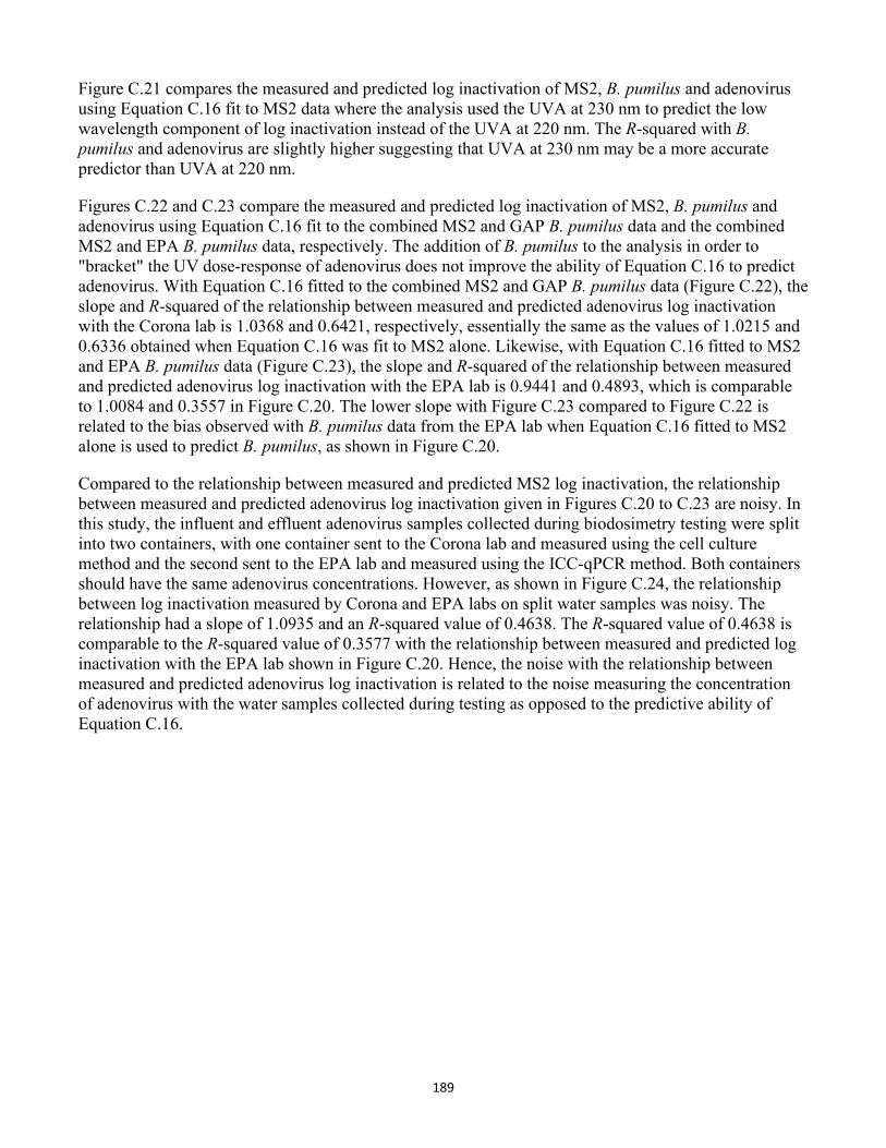
189

Figure C.21 compares the measured and predicted log inactivation of MS2, B. pumilus and adenovirus using Equation C.16 fit to MS2 data where the analysis used the UVA at 230 nm to predict the low wavelength component of log inactivation instead of the UVA at 220 nm. The R-squared with B. pumilus and adenovirus are slightly higher suggesting that UVA at 230 nm may be a more accurate predictor than UVA at 220 nm.

Figures C.22 and C.23 compare the measured and predicted log inactivation of MS2, B. pumilus and adenovirus using Equation C.16 fit to the combined MS2 and GAP B. pumilus data and the combined MS2 and EPA B. pumilus data, respectively. The addition of B. pumilus to the analysis in order to "bracket" the UV dose-response of adenovirus does not improve the ability of Equation C.16 to predict adenovirus. With Equation C.16 fitted to the combined MS2 and GAP B. pumilus data (Figure C.22), the slope and R-squared of the relationship between measured and predicted adenovirus log inactivation with the Corona lab is 1.0368 and 0.6421, respectively, essentially the same as the values of 1.0215 and 0.6336 obtained when Equation C.16 was fit to MS2 alone. Likewise, with Equation C.16 fitted to MS2 and EPA B. pumilus data (Figure C.23), the slope and R-squared of the relationship between measured and predicted adenovirus log inactivation with the EPA lab is 0.9441 and 0.4893, which is comparable to 1.0084 and 0.3557 in Figure C.20. The lower slope with Figure C.23 compared to Figure C.22 is related to the bias observed with B. pumilus data from the EPA lab when Equation C.16 fitted to MS2 alone is used to predict B. pumilus, as shown in Figure C.20.

Compared to the relationship between measured and predicted MS2 log inactivation, the relationship between measured and predicted adenovirus log inactivation given in Figures C.20 to C.23 are noisy. In this study, the influent and effluent adenovirus samples collected during biodosimetry testing were split into two containers, with one container sent to the Corona lab and measured using the cell culture method and the second sent to the EPA lab and measured using the ICC-qPCR method. Both containers should have the same adenovirus concentrations. However, as shown in Figure C.24, the relationship between log inactivation measured by Corona and EPA labs on split water samples was noisy. The relationship had a slope of 1.0935 and an R-squared value of 0.4638. The R-squared value of 0.4638 is comparable to the R-squared value of 0.3577 with the relationship between measured and predicted log inactivation with the EPA lab shown in Figure C.20. Hence, the noise with the relationship between measured and predicted adenovirus log inactivation is related to the noise measuring the concentration of adenovirus with the water samples collected during testing as opposed to the predictive ability of Equation C.16.

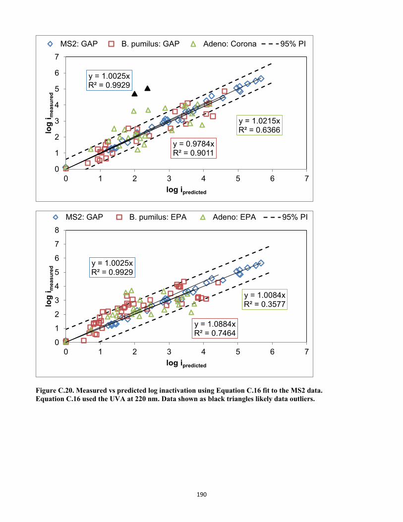
190

y = 1.0025xR² = 0.9929

y = 0.9784xR² = 0.9011

y = 1.0215xR² = 0.6366

0

1

2

3

4

5

6

7

0 1 2 3 4 5 6 7

log

i mea

sure

d

log ipredicted

MS2: GAP B. pumilus: GAP Adeno: Corona 95% PI

y = 1.0025xR² = 0.9929

y = 1.0884xR² = 0.7464

y = 1.0084xR² = 0.3577

0

1

2

3

4

5

6

7

8

0 1 2 3 4 5 6 7

log

i mea

sure

d

log ipredicted

MS2: GAP B. pumilus: EPA Adeno: EPA 95% PI

Figure C.20. Measured vs predicted log inactivation using Equation C.16 fit to the MS2 data. Equation C.16 used the UVA at 220 nm. Data shown as black triangles likely data outliers.

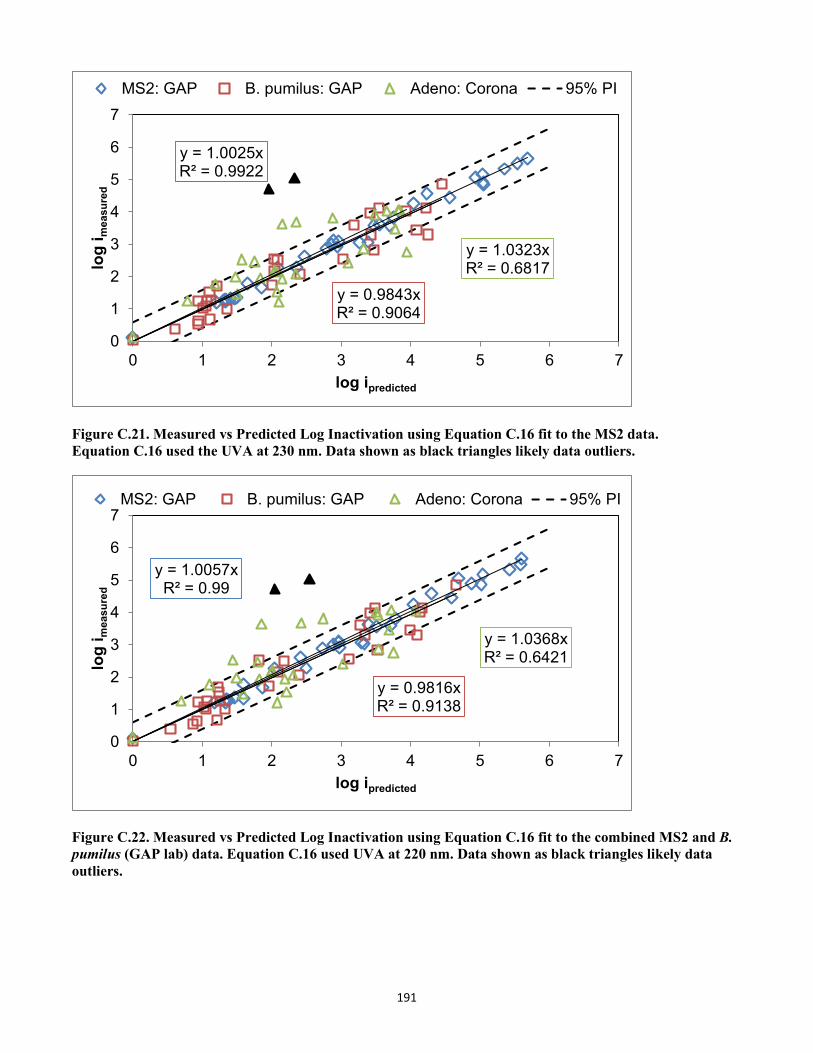
191

y = 1.0025xR² = 0.9922

y = 0.9843xR² = 0.9064

y = 1.0323xR² = 0.6817

0

1

2

3

4

5

6

7

0 1 2 3 4 5 6 7

log

i mea

sure

d

log ipredicted


Figure C.21. Measured vs Predicted Log Inactivation using Equation C.16 fit to the MS2 data. Equation C.16 used the UVA at 230 nm. Data shown as black triangles likely data outliers.

y = 1.0057xR² = 0.99

y = 0.9816xR² = 0.9138

y = 1.0368xR² = 0.6421

0

1

2

3

4

5

6

7

0 1 2 3 4 5 6 7

log

i mea

sure

d

log ipredicted


Figure C.22. Measured vs Predicted Log Inactivation using Equation C.16 fit to the combined MS2 and B. pumilus (GAP lab) data. Equation C.16 used UVA at 220 nm. Data shown as black triangles likely data outliers.

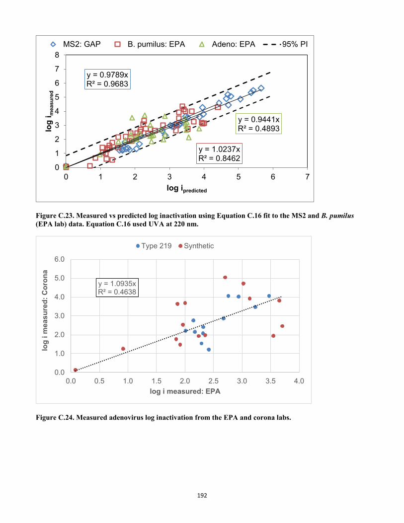
192

y = 0.9789xR² = 0.9683

y = 1.0237xR² = 0.8462

y = 0.9441xR² = 0.4893

0

1

2

3

4

5

6

7

8

0 1 2 3 4 5 6 7

log

i mea

sure

d

log ipredicted

MS2: GAP B. pumilus: EPA Adeno: EPA 95% PI

Figure C.23. Measured vs predicted log inactivation using Equation C.16 fit to the MS2 and B. pumilus (EPA lab) data. Equation C.16 used UVA at 220 nm.

y = 1.0935xR² = 0.4638

0.0

1.0

2.0

3.0

4.0

5.0

6.0

0.0 0.5 1.0 1.5 2.0 2.5 3.0 3.5 4.0

log

i mea

sure

d: C

oron

a

log i measured: EPA

Type 219 Synthetic

Figure C.24. Measured adenovirus log inactivation from the EPA and corona labs.

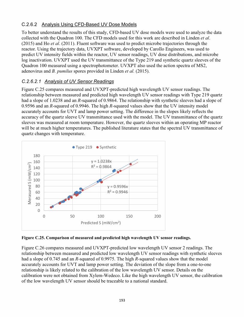
193

C.2.6.2 Analysis Using CFD-Based UV Dose Models To better understand the results of this study, CFD-based UV dose models were used to analyze the data collected with the Quadron 100. The CFD models used for this work are described in Linden et al. (2015) and Ho et al. (2011). Fluent software was used to predict microbe trajectories through the reactor. Using the trajectory data, UVXPT software, developed by Carollo Engineers, was used to predict UV intensity fields within the reactor, UV sensor readings, UV dose distributions, and microbe log inactivation. UVXPT used the UV transmittance of the Type 219 and synthetic quartz sleeves of the Quadron 100 measured using a spectrophotometer. UVXPT also used the action spectra of MS2, adenovirus and B. pumilus spores provided in Linden et al. (2015).

C.2.6.2.1 Analysis of UV Sensor Readings Figure C.25 compares measured and UVXPT-predicted high wavelength UV sensor readings. The relationship between measured and predicted high wavelength UV sensor readings with Type 219 quartz had a slope of 1.0238 and an R-squared of 0.9864. The relationship with synthetic sleeves had a slope of 0.9596 and an R-squared of 0.9946. The high R-squared values show that the UV intensity model accurately accounts for UVT and lamp power setting. The difference in the slopes likely reflects the accuracy of the quartz sleeve UV transmittance used with the model. The UV transmittance of the quartz sleeves was measured at room temperature. However, the quartz sleeves within an operating MP reactor will be at much higher temperatures. The published literature states that the spectral UV transmittance of quartz changes with temperature.

Figure C.25. Comparison of measured and predicted high wavelength UV sensor readings.

Figure C.26 compares measured and UVXPT-predicted low wavelength UV sensor 2 readings. The relationship between measured and predicted low wavelength UV sensor readings with synthetic sleeves had a slope of 0.745 and an R-squared of 0.9975. The high R-squared values show that the model accurately accounts for UVT and lamp power setting. The deviation of the slope from a one-to-one relationship is likely related to the calibration of the low wavelength UV sensor. Details on the calibration were not obtained from Xylem-Wedeco. Like the high wavelength UV sensor, the calibration of the low wavelength UV sensor should be traceable to a national standard.

y = 1.0238xR² = 0.9864

y = 0.9596xR² = 0.9946

020406080

100120140160180

0 50 100 150 200

Mer

asur

ed S

(mW

/cm

2 )

Predicted S (mW/cm2)

Type 219 Synthetic

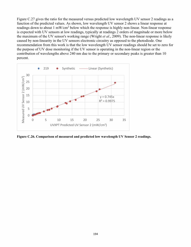
194

Figure C.27 gives the ratio for the measured versus predicted low wavelength UV sensor 2 readings as a function of the predicted values. As shown, low wavelength UV sensor 2 shows a linear response at readings down to about 1 mW/cm2 below which the response is highly non-linear. Non-linear response is expected with UV sensors at low readings, typically at readings 2 orders of magnitude or more below the maximum of the UV sensor's working range (Wright et al., 2009). The non-linear response is likely caused by non-linearity in the UV sensors electronic circuitry as opposed to the photodiode. One recommendation from this work is that the low wavelength UV sensor readings should be set to zero for the purpose of UV dose monitoring if the UV sensor is operating in the non-linear region or the contribution of wavelengths above 240 nm due to the primary or secondary peaks is greater than 10 percent.

y = 0.745xR² = 0.9975

0

5

10

15

20

25

30

0 5 10 15 20 25 30 35

Mea

sure

d U

V Se

nsor

2 (m

W/c

m2 )

UVXPT Predicted UV Sensor 2 (mW/cm2)

219 Synthetic Linear (Synthetic)

Figure C.26. Comparison of measured and predicted low wavelength UV Sensor 2 readings.

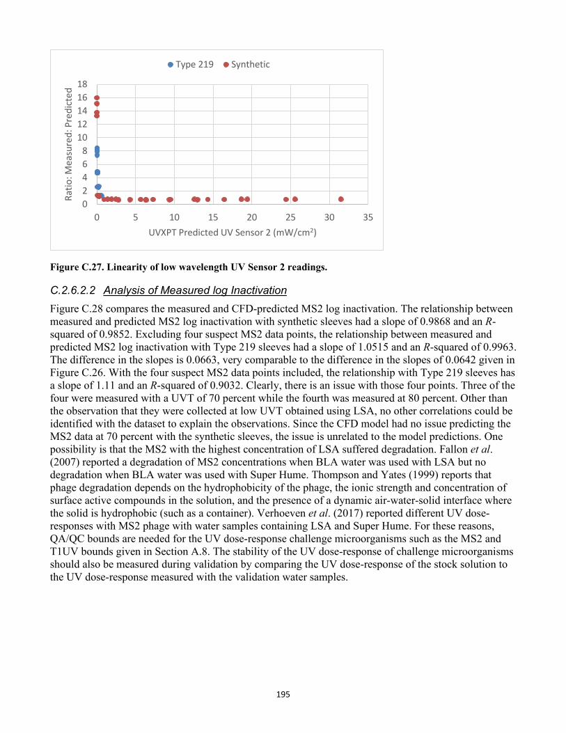
195

02468

1012141618

0 5 10 15 20 25 30 35

Ratio

: Mea

sure

d: P

redi

cted

UVXPT Predicted UV Sensor 2 (mW/cm2)

Type 219 Synthetic

Figure C.27. Linearity of low wavelength UV Sensor 2 readings.

C.2.6.2.2 Analysis of Measured log Inactivation Figure C.28 compares the measured and CFD-predicted MS2 log inactivation. The relationship between measured and predicted MS2 log inactivation with synthetic sleeves had a slope of 0.9868 and an R-squared of 0.9852. Excluding four suspect MS2 data points, the relationship between measured and predicted MS2 log inactivation with Type 219 sleeves had a slope of 1.0515 and an R-squared of 0.9963. The difference in the slopes is 0.0663, very comparable to the difference in the slopes of 0.0642 given in Figure C.26. With the four suspect MS2 data points included, the relationship with Type 219 sleeves has a slope of 1.11 and an R-squared of 0.9032. Clearly, there is an issue with those four points. Three of the four were measured with a UVT of 70 percent while the fourth was measured at 80 percent. Other than the observation that they were collected at low UVT obtained using LSA, no other correlations could be identified with the dataset to explain the observations. Since the CFD model had no issue predicting the MS2 data at 70 percent with the synthetic sleeves, the issue is unrelated to the model predictions. One possibility is that the MS2 with the highest concentration of LSA suffered degradation. Fallon et al. (2007) reported a degradation of MS2 concentrations when BLA water was used with LSA but no degradation when BLA water was used with Super Hume. Thompson and Yates (1999) reports that phage degradation depends on the hydrophobicity of the phage, the ionic strength and concentration of surface active compounds in the solution, and the presence of a dynamic air-water-solid interface where the solid is hydrophobic (such as a container). Verhoeven et al. (2017) reported different UV dose-responses with MS2 phage with water samples containing LSA and Super Hume. For these reasons, QA/QC bounds are needed for the UV dose-response challenge microorganisms such as the MS2 and T1UV bounds given in Section A.8. The stability of the UV dose-response of challenge microorganisms should also be measured during validation by comparing the UV dose-response of the stock solution to the UV dose-response measured with the validation water samples.

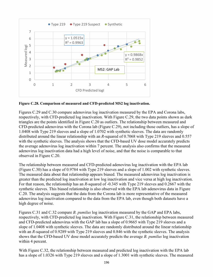
196

y = 1.0515xR² = 0.9963

y = 0.9868xR² = 0.9852

0

1

2

3

4

5

6

7

0 1 2 3 4 5 6

Mea

sure

d lo

gI

CFD Predicted logI

Type 219 Type 219 Suspect Synthetic

MS2: GAP Lab

Figure C.28. Comparison of measured and CFD-predicted MS2 log inactivation.

Figures C.29 and C.30 compare adenovirus log inactivation measured by the EPA and Corona labs, respectively, with CFD-predicted log inactivation. With Figure C.29, the two data points shown as dark triangles are the points identified in Figure C.20 as outliers. The relationship between measured and CFD-predicted adenovirus with the Corona lab (Figure C.29), not including those outliers, has a slope of 1.0408 with Type 219 sleeves and a slope of 1.0702 with synthetic sleeves. The data are randomly distributed around the linear relationship with an R-squared of 0.7068 with Type 219 sleeves and 0.557 with the synthetic sleeves. The analysis shows that the CFD-based UV dose model accurately predicts the average adenovirus log inactivation within 7 percent. The analysis also confirms that the measured adenovirus log inactivation data had a high level of noise, and that the noise is comparable to that observed in Figure C.20.

The relationship between measured and CFD-predicted adenovirus log inactivation with the EPA lab (Figure C.30) has a slope of 0.9784 with Type 219 sleeves and a slope of 1.002 with synthetic sleeves. The measured data about that relationship appears biased. The measured adenovirus log inactivation is greater than the predicted log inactivation at low log inactivation and vice versa at high log inactivation. For that reason, the relationship has an R-squared of -0.345 with Type 219 sleeves and 0.2667 with the synthetic sleeves. This biased relationship is also observed with the EPA lab adenovirus data in Figure C.20. The analysis suggests that the data from the Corona lab is more representative of the measured adenovirus log inactivation compared to the data from the EPA lab, even though both datasets have a high degree of noise.

Figures C.31 and C.32 compare B. pumilus log inactivation measured by the GAP and EPA labs, respectively, with CFD-predicted log inactivation. With Figure C.31, the relationship between measured and CFD-predicted adenovirus with the GAP lab has a slope of 0.9665 with Type 219 sleeves and a slope of 1.0408 with synthetic sleeves. The data are randomly distributed around the linear relationship with an R-squared of 0.9289 with Type 219 sleeves and 0.846 with the synthetic sleeves. The analysis shows that the CFD-based UV dose model accurately predicts the average B. pumilus log inactivation within 4 percent.

With Figure C.32, the relationship between measured and predicted log inactivation with the EPA lab has a slope of 1.0326 with Type 219 sleeves and a slope of 1.3001 with synthetic sleeves. The measured

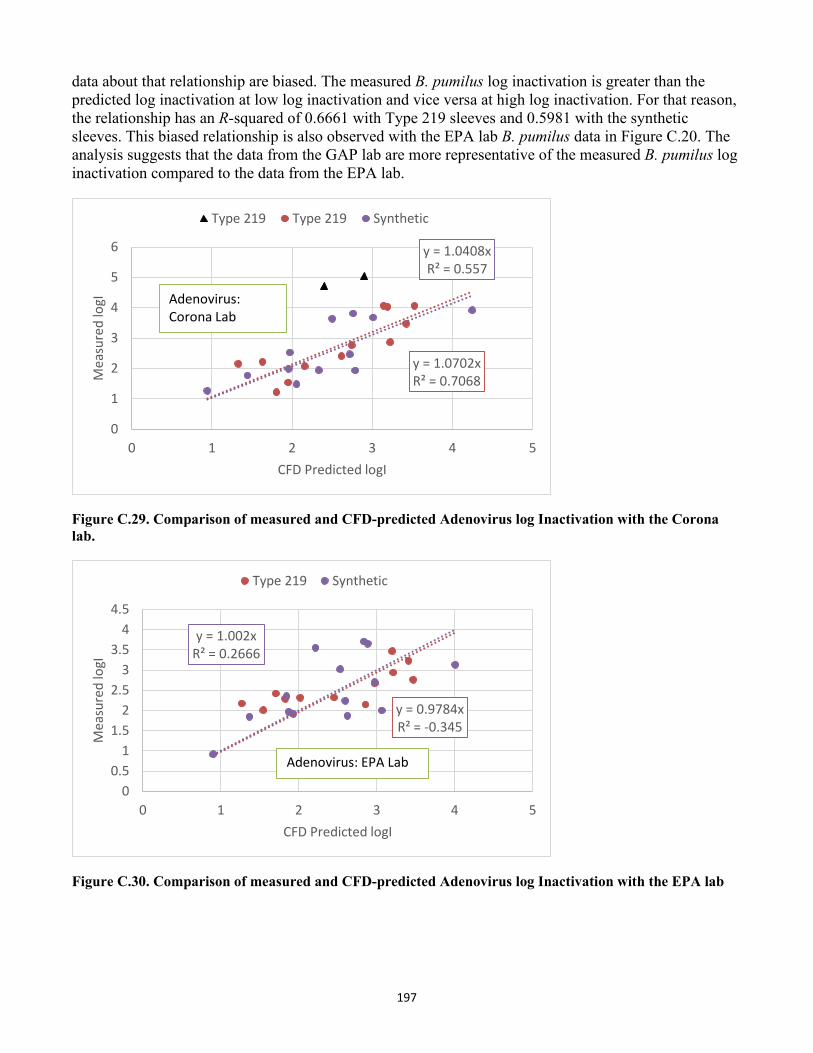
197

data about that relationship are biased. The measured B. pumilus log inactivation is greater than the predicted log inactivation at low log inactivation and vice versa at high log inactivation. For that reason, the relationship has an R-squared of 0.6661 with Type 219 sleeves and 0.5981 with the synthetic sleeves. This biased relationship is also observed with the EPA lab B. pumilus data in Figure C.20. The analysis suggests that the data from the GAP lab are more representative of the measured B. pumilus log inactivation compared to the data from the EPA lab.

y = 1.0702xR² = 0.7068

y = 1.0408xR² = 0.557

0

1

2

3

4

5

6

0 1 2 3 4 5

Mea

sure

d lo

gI

CFD Predicted logI

Type 219 Type 219 Synthetic

Adenovirus:Corona Lab

Figure C.29. Comparison of measured and CFD-predicted Adenovirus log Inactivation with the Corona lab.

y = 0.9784xR² = -0.345

y = 1.002xR² = 0.2666

00.5

11.5

22.5

33.5

44.5

0 1 2 3 4 5

Mea

sure

d lo

gI

CFD Predicted logI

Type 219 Synthetic

Adenovirus: EPA Lab

Figure C.30. Comparison of measured and CFD-predicted Adenovirus log Inactivation with the EPA lab

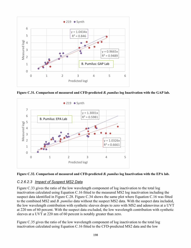
198

y = 0.9665xR² = 0.9489

y = 1.0434xR² = 0.846

0

1

2

3

4

5

6

0 1 2 3 4 5 6

Mea

sure

d lo

gI

Predicted logI

219 Synth

B. Pumilus: GAP Lab

Figure C.31. Comparison of measured and CFD-predicted B. pumilus log Inactivation with the GAP lab.

y = 1.0326xR² = 0.6661

y = 1.3001xR² = 0.5981

0

1

2

3

4

5

6

7

0 1 2 3 4 5

Mea

sure

d lo

gI

Predicted logI

219 Synth

B. Pumilus: EPA Lab

Figure C.32. Comparison of measured and CFD-predicted B. pumilus log Inactivation with the EPA lab.

C.2.6.2.3 Impact of Suspect MS2 Data Figure C.33 gives the ratio of the low wavelength component of log inactivation to the total log inactivation calculated using Equation C.16 fitted to the measured MS2 log inactivation including the suspect data identified in Figure C.28. Figure C.34 shows the same plot where Equation C.16 was fitted to the combined MS2 and B. pumilus data without the suspect MS2 data. With the suspect data included, the low wavelength contribution with synthetic sleeves drops to zero with MS2 and adenovirus at a UVT at 220 nm of 60 percent. With the suspect data excluded, the low wavelength contribution with synthetic sleeves at a UVT at 220 nm of 60 percent is notably greater than zero.

Figure C.35 gives the ratio of the low wavelength component of log inactivation to the total log inactivation calculated using Equation C.16 fitted to the CFD-predicted MS2 data and the low

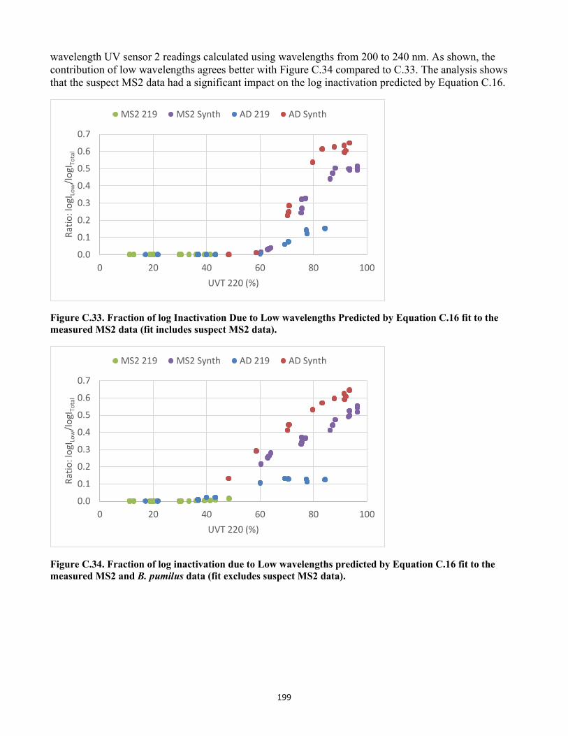
199

wavelength UV sensor 2 readings calculated using wavelengths from 200 to 240 nm. As shown, the contribution of low wavelengths agrees better with Figure C.34 compared to C.33. The analysis shows that the suspect MS2 data had a significant impact on the log inactivation predicted by Equation C.16.

0.0

0.1

0.2

0.3

0.4

0.5

0.6

0.7

0 20 40 60 80 100

Ratio

: log

I Low

/logI

Tota

l

UVT 220 (%)

MS2 219 MS2 Synth AD 219 AD Synth

Figure C.33. Fraction of log Inactivation Due to Low wavelengths Predicted by Equation C.16 fit to the measured MS2 data (fit includes suspect MS2 data).

0.0

0.1

0.2

0.3

0.4

0.5

0.6

0.7

0 20 40 60 80 100

Ratio

: log

I Low

/logI

Tota

l

UVT 220 (%)


Figure C.34. Fraction of log inactivation due to Low wavelengths predicted by Equation C.16 fit to the measured MS2 and B. pumilus data (fit excludes suspect MS2 data).

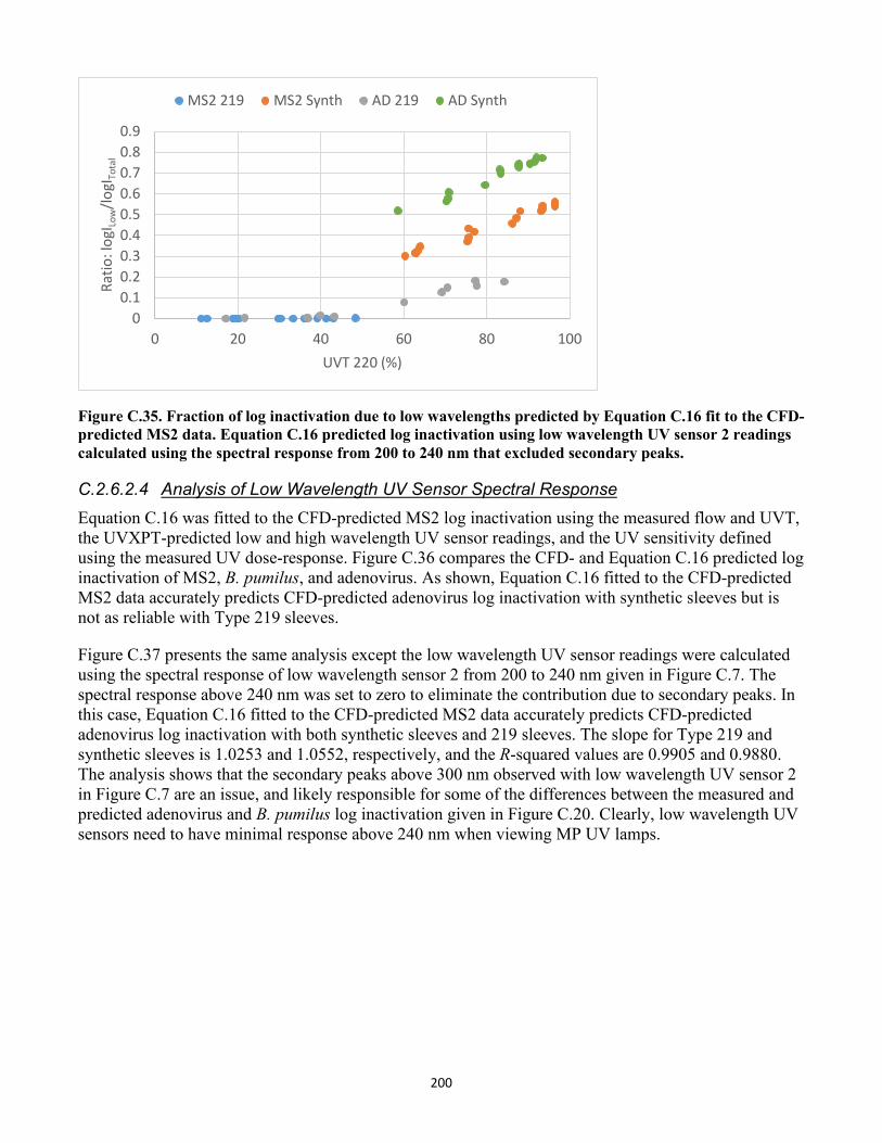
200

00.10.20.30.40.50.60.70.80.9

0 20 40 60 80 100

Ratio

: log

I Low

/logI

Tota

l

UVT 220 (%)


Figure C.35. Fraction of log inactivation due to low wavelengths predicted by Equation C.16 fit to the CFD-predicted MS2 data. Equation C.16 predicted log inactivation using low wavelength UV sensor 2 readings calculated using the spectral response from 200 to 240 nm that excluded secondary peaks.

C.2.6.2.4 Analysis of Low Wavelength UV Sensor Spectral Response Equation C.16 was fitted to the CFD-predicted MS2 log inactivation using the measured flow and UVT, the UVXPT-predicted low and high wavelength UV sensor readings, and the UV sensitivity defined using the measured UV dose-response. Figure C.36 compares the CFD- and Equation C.16 predicted log inactivation of MS2, B. pumilus, and adenovirus. As shown, Equation C.16 fitted to the CFD-predicted MS2 data accurately predicts CFD-predicted adenovirus log inactivation with synthetic sleeves but is not as reliable with Type 219 sleeves.

Figure C.37 presents the same analysis except the low wavelength UV sensor readings were calculated using the spectral response of low wavelength sensor 2 from 200 to 240 nm given in Figure C.7. The spectral response above 240 nm was set to zero to eliminate the contribution due to secondary peaks. In this case, Equation C.16 fitted to the CFD-predicted MS2 data accurately predicts CFD-predicted adenovirus log inactivation with both synthetic sleeves and 219 sleeves. The slope for Type 219 and synthetic sleeves is 1.0253 and 1.0552, respectively, and the R-squared values are 0.9905 and 0.9880. The analysis shows that the secondary peaks above 300 nm observed with low wavelength UV sensor 2 in Figure C.7 are an issue, and likely responsible for some of the differences between the measured and predicted adenovirus and B. pumilus log inactivation given in Figure C.20. Clearly, low wavelength UV sensors need to have minimal response above 240 nm when viewing MP UV lamps.

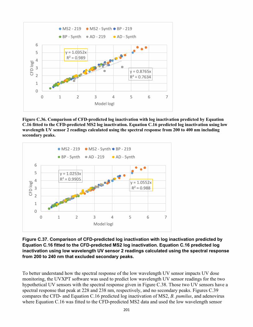
201

y = 0.8765xR² = 0.7634

y = 1.0352xR² = 0.989

0

1

2

3

4

5

6

0 1 2 3 4 5 6 7

CFD

logI

Model logI

MS2 - 219 MS2 - Synth BP - 219

BP - Synth AD - 219 AD - Synth

Figure C.36. Comparison of CFD-predicted log inactivation with log inactivation predicted by Equation C.16 fitted to the CFD-predicted MS2 log inactivation. Equation C.16 predicted log inactivation using low wavelength UV sensor 2 readings calculated using the spectral response from 200 to 400 nm including secondary peaks.

y = 1.0253xR² = 0.9905

y = 1.0552xR² = 0.988

0

1

2

3

4

5

6

0 1 2 3 4 5 6 7

CFD

logI

Model logI

MS2 - 219 MS2 - Synth BP - 219


Figure C.37. Comparison of CFD-predicted log inactivation with log inactivation predicted by Equation C.16 fitted to the CFD-predicted MS2 log inactivation. Equation C.16 predicted log inactivation using low wavelength UV sensor 2 readings calculated using the spectral response from 200 to 240 nm that excluded secondary peaks.

To better understand how the spectral response of the low wavelength UV sensor impacts UV dose monitoring, the UVXPT software was used to predict low wavelength UV sensor readings for the two hypothetical UV sensors with the spectral response given in Figure C.38. Those two UV sensors have a spectral response that peak at 228 and 238 nm, respectively, and no secondary peaks. Figures C.39 compares the CFD- and Equation C.16 predicted log inactivation of MS2, B. pumilus, and adenovirus where Equation C.16 was fitted to the CFD-predicted MS2 data and used the low wavelength sensor

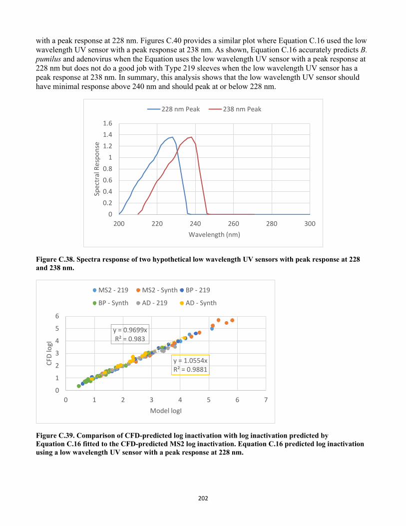
202

with a peak response at 228 nm. Figures C.40 provides a similar plot where Equation C.16 used the low wavelength UV sensor with a peak response at 238 nm. As shown, Equation C.16 accurately predicts B. pumilus and adenovirus when the Equation uses the low wavelength UV sensor with a peak response at 228 nm but does not do a good job with Type 219 sleeves when the low wavelength UV sensor has a peak response at 238 nm. In summary, this analysis shows that the low wavelength UV sensor should have minimal response above 240 nm and should peak at or below 228 nm.

00.20.40.60.8

11.21.41.6

200 220 240 260 280 300

Spec

tral

Res

pons

e

Wavelength (nm)

228 nm Peak 238 nm Peak

Figure C.38. Spectra response of two hypothetical low wavelength UV sensors with peak response at 228 and 238 nm.

y = 0.9699xR² = 0.983

y = 1.0554xR² = 0.9881

0

1

2

3

4

5

6

0 1 2 3 4 5 6 7

CFD

logI

Model logI

MS2 - 219 MS2 - Synth BP - 219


Figure C.39. Comparison of CFD-predicted log inactivation with log inactivation predicted by Equation C.16 fitted to the CFD-predicted MS2 log inactivation. Equation C.16 predicted log inactivation using a low wavelength UV sensor with a peak response at 228 nm.

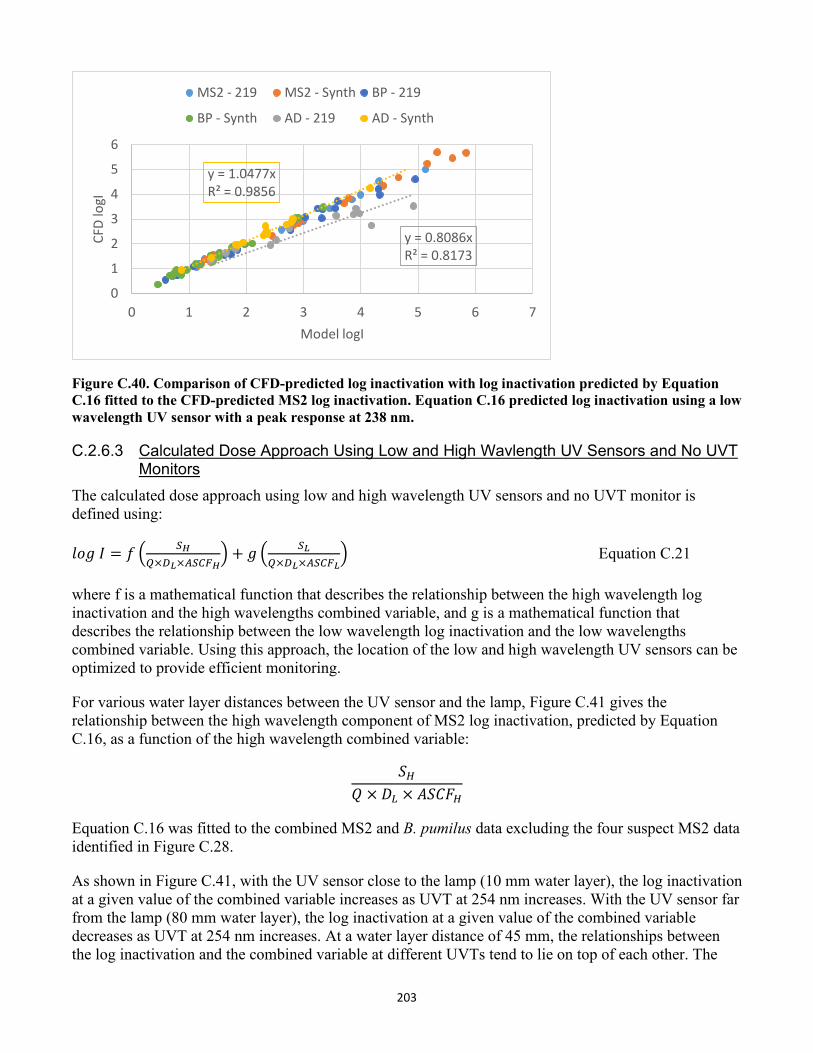
203

y = 0.8086xR² = 0.8173

y = 1.0477xR² = 0.9856

0

1

2

3

4

5

6

0 1 2 3 4 5 6 7

CFD

logI

Model logI

MS2 - 219 MS2 - Synth BP - 219


Figure C.40. Comparison of CFD-predicted log inactivation with log inactivation predicted by Equation C.16 fitted to the CFD-predicted MS2 log inactivation. Equation C.16 predicted log inactivation using a low wavelength UV sensor with a peak response at 238 nm.

C.2.6.3 Calculated Dose Approach Using Low and High Wavlength UV Sensors and No UVT Monitors

The calculated dose approach using low and high wavelength UV sensors and no UVT monitor is defined using:

𝑉𝑉𝐷𝐷𝑙𝑙 𝐼𝐼 = 𝑓𝑓 � 𝑆𝑆𝐻𝐻𝑄𝑄×𝑅𝑅𝐿𝐿×𝐴𝐴𝑆𝑆𝐶𝐶𝐹𝐹𝐻𝐻

� + 𝑙𝑙 � 𝑆𝑆𝐿𝐿𝑄𝑄×𝑅𝑅𝐿𝐿×𝐴𝐴𝑆𝑆𝐶𝐶𝐹𝐹𝐿𝐿

� Equation C.21

where f is a mathematical function that describes the relationship between the high wavelength log inactivation and the high wavelengths combined variable, and g is a mathematical function that describes the relationship between the low wavelength log inactivation and the low wavelengths combined variable. Using this approach, the location of the low and high wavelength UV sensors can be optimized to provide efficient monitoring.

For various water layer distances between the UV sensor and the lamp, Figure C.41 gives the relationship between the high wavelength component of MS2 log inactivation, predicted by Equation C.16, as a function of the high wavelength combined variable:


Equation C.16 was fitted to the combined MS2 and B. pumilus data excluding the four suspect MS2 data identified in Figure C.28.

As shown in Figure C.41, with the UV sensor close to the lamp (10 mm water layer), the log inactivation at a given value of the combined variable increases as UVT at 254 nm increases. With the UV sensor far from the lamp (80 mm water layer), the log inactivation at a given value of the combined variable decreases as UVT at 254 nm increases. At a water layer distance of 45 mm, the relationships between the log inactivation and the combined variable at different UVTs tend to lie on top of each other. The

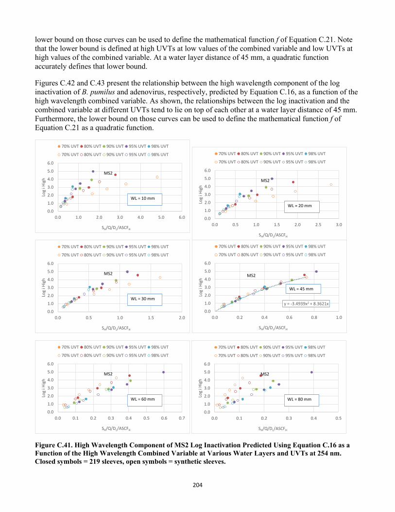
204

lower bound on those curves can be used to define the mathematical function f of Equation C.21. Note that the lower bound is defined at high UVTs at low values of the combined variable and low UVTs at high values of the combined variable. At a water layer distance of 45 mm, a quadratic function accurately defines that lower bound.

Figures C.42 and C.43 present the relationship between the high wavelength component of the log inactivation of B. pumilus and adenovirus, respectively, predicted by Equation C.16, as a function of the high wavelength combined variable. As shown, the relationships between the log inactivation and the combined variable at different UVTs tend to lie on top of each other at a water layer distance of 45 mm. Furthermore, the lower bound on those curves can be used to define the mathematical function f of Equation C.21 as a quadratic function.

0.0

1.0

2.0

3.0

4.0

5.0

6.0

0.0 1.0 2.0 3.0 4.0 5.0 6.0

Log

i Hig

h

SH/Q/DL/ASCFH



MS2

WL = 10 mm

0.0

1.0

2.0

3.0

4.0

5.0

6.0

0.0 0.5 1.0 1.5 2.0

Log

i Hig

h

SH/Q/DL/ASCFH



MS2

WL = 30 mm

0.0

1.0

2.0

3.0

4.0

5.0

6.0

0.0 0.1 0.2 0.3 0.4 0.5 0.6 0.7

Log

i Hig

h

SH/Q/DL/ASCFH



MS2

WL = 60 mm

0.0

1.0

2.0

3.0

4.0

5.0

6.0

0.0 0.5 1.0 1.5 2.0 2.5 3.0

Log

i Hig

h

SH/Q/DL/ASCFH



MS2

WL = 20 mm

y = -3.4939x2 + 8.3621x

0.0

1.0

2.0

3.0

4.0

5.0

6.0

0.0 0.2 0.4 0.6 0.8 1.0

Log

i Hig

h

SH/Q/DL/ASCFH



MS2

WL = 45 mm

0.0

1.0

2.0

3.0

4.0

5.0

6.0

0.0 0.1 0.2 0.3 0.4 0.5

Log

i Hig

h

SH/Q/DL/ASCFH



MS2

WL = 80 mm

Figure C.41. High Wavelength Component of MS2 Log Inactivation Predicted Using Equation C.16 as a Function of the High Wavelength Combined Variable at Various Water Layers and UVTs at 254 nm. Closed symbols = 219 sleeves, open symbols = synthetic sleeves.

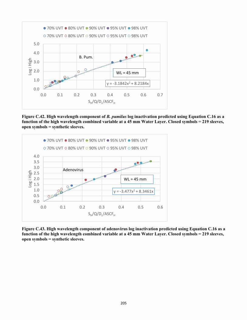
205

y = -3.1842x2 + 8.2184x0.0

1.0

2.0

3.0

4.0

5.0

0.0 0.1 0.2 0.3 0.4 0.5 0.6 0.7

Log

i Hig

h

SH/Q/DL/ASCFH



B. Pum.

WL = 45 mm

Figure C.42. High wavelength component of B. pumilus log inactivation predicted using Equation C.16 as a function of the high wavelength combined variable at a 45 mm Water Layer. Closed symbols = 219 sleeves, open symbols = synthetic sleeves.

y = -3.477x2 + 8.3461x

0.00.51.01.52.02.53.03.54.0

0.0 0.1 0.2 0.3 0.4 0.5 0.6

Log

i Hig

h

SH/Q/DL/ASCFH



Adenovirus

WL = 45 mm

Figure C.43. High wavelength component of adenovirus log inactivation predicted using Equation C.16 as a function of the high wavelength combined variable at a 45 mm Water Layer. Closed symbols = 219 sleeves, open symbols = synthetic sleeves.

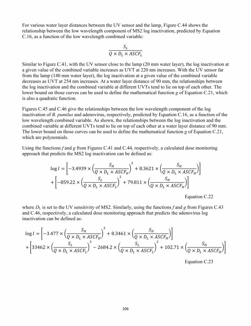
206

For various water layer distances between the UV sensor and the lamp, Figure C.44 shows the relationship between the low wavelength component of MS2 log inactivation, predicted by Equation C.16, as a function of the low wavelength combined variable:


Similar to Figure C.41, with the UV sensor close to the lamp (20 mm water layer), the log inactivation at a given value of the combined variable increases as UVT at 220 nm increases. With the UV sensor far from the lamp (140 mm water layer), the log inactivation at a given value of the combined variable decreases as UVT at 254 nm increases. At a water layer distance of 90 mm, the relationships between the log inactivation and the combined variable at different UVTs tend to lie on top of each other. The lower bound on those curves can be used to define the mathematical function g of Equation C.21, which is also a quadratic function.

Figures C.45 and C.46 give the relationships between the low wavelength component of the log inactivation of B. pumilus and adenovirus, respectively, predicted by Equation C.16, as a function of the low wavelength combined variable. As shown, the relationships between the log inactivation and the combined variable at different UVTs tend to lie on top of each other at a water layer distance of 90 mm. The lower bound on those curves can be used to define the mathematical function g of Equation C.21, which are polynomials.

Using the functions f and g from Figures C.41 and C.44, respectively, a calculated dose monitoring approach that predicts the MS2 log inactivation can be defined as:

log 𝐼𝐼 = �−3.4939 × �𝑆𝑆𝐻𝐻

𝑄𝑄 × 𝐷𝐷𝐿𝐿 × 𝐴𝐴𝑆𝑆𝐴𝐴𝑉𝑉𝐻𝐻�2

+ 8.3621 × �𝑆𝑆𝐻𝐻

𝑄𝑄 × 𝐷𝐷𝐿𝐿 × 𝐴𝐴𝑆𝑆𝐴𝐴𝑉𝑉𝐻𝐻��

+ �−859.22 × �𝑆𝑆𝐿𝐿


+ 79.811 × �𝑆𝑆𝐻𝐻


Equation C.22

where DL is set to the UV sensitivity of MS2. Similarly, using the functions f and g from Figures C.43 and C.46, respectively, a calculated dose monitoring approach that predicts the adenovirus log inactivation can be defined as:

log 𝐼𝐼 = �−3.477 × �𝑆𝑆𝐻𝐻

𝑄𝑄 × 𝐷𝐷𝐿𝐿 × 𝐴𝐴𝑆𝑆𝐴𝐴𝑉𝑉𝐻𝐻�2

+ 8.3461 × �𝑆𝑆𝐻𝐻


+ �33462 × �𝑆𝑆𝐿𝐿


− 2684.2 × �𝑆𝑆𝐿𝐿


+ 102.71 × �𝑆𝑆𝐻𝐻


Equation C.23

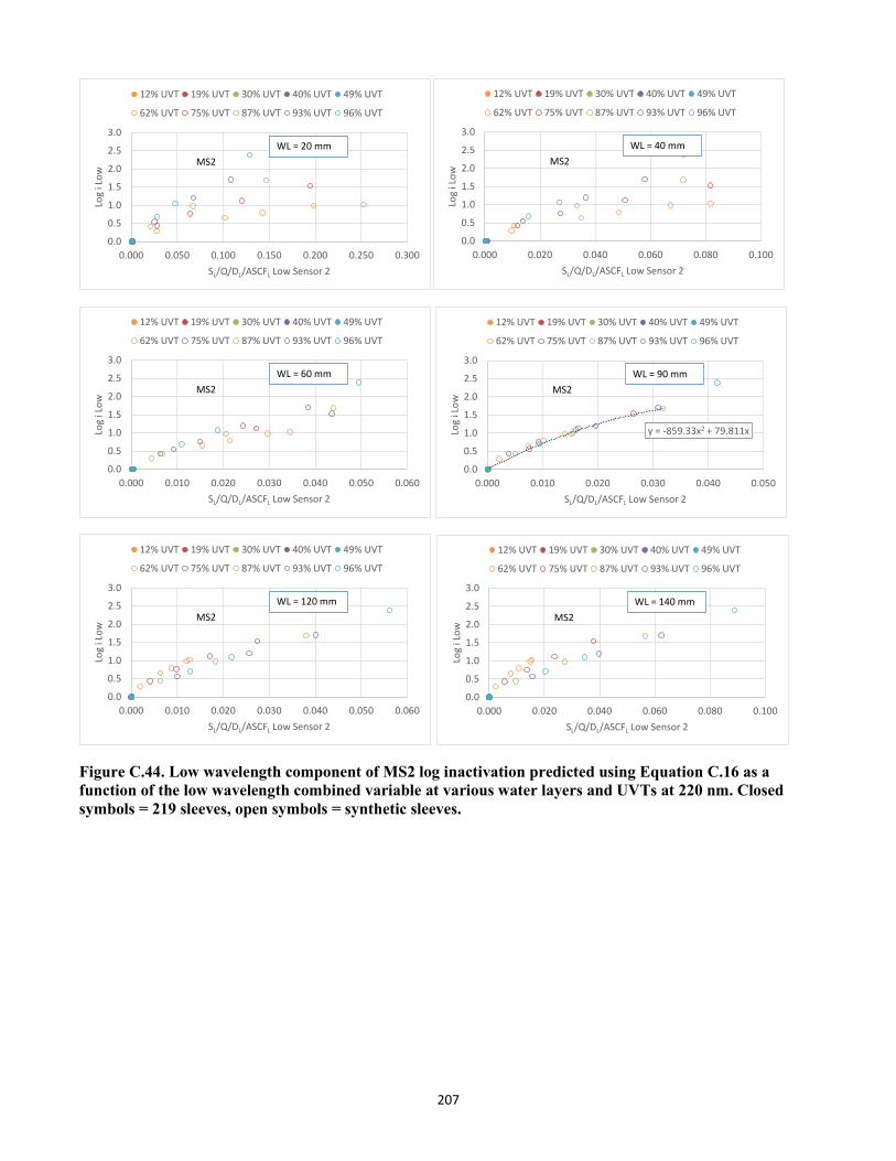
207

0.0

0.5

1.0

1.5

2.0

2.5

3.0

0.000 0.050 0.100 0.150 0.200 0.250 0.300

Log

i Low

SL/Q/DL/ASCFL Low Sensor 2



MS2WL = 20 mm

0.0

0.5

1.0

1.5

2.0

2.5

3.0

0.000 0.010 0.020 0.030 0.040 0.050 0.060

Log

i Low




MS2WL = 60 mm

0.0

0.5

1.0

1.5

2.0

2.5

3.0

0.000 0.010 0.020 0.030 0.040 0.050 0.060

Log

i Low




MS2WL = 120 mm

0.0

0.5

1.0

1.5

2.0

2.5

3.0

0.000 0.020 0.040 0.060 0.080 0.100

Log

i Low




MS2WL = 40 mm

y = -859.33x2 + 79.811x

0.0

0.5

1.0

1.5

2.0

2.5

3.0

0.000 0.010 0.020 0.030 0.040 0.050

Log

i Low




MS2WL = 90 mm

0.0

0.5

1.0

1.5

2.0

2.5

3.0

0.000 0.020 0.040 0.060 0.080 0.100

Log

i Low




MS2WL = 140 mm

Figure C.44. Low wavelength component of MS2 log inactivation predicted using Equation C.16 as a function of the low wavelength combined variable at various water layers and UVTs at 220 nm. Closed symbols = 219 sleeves, open symbols = synthetic sleeves.

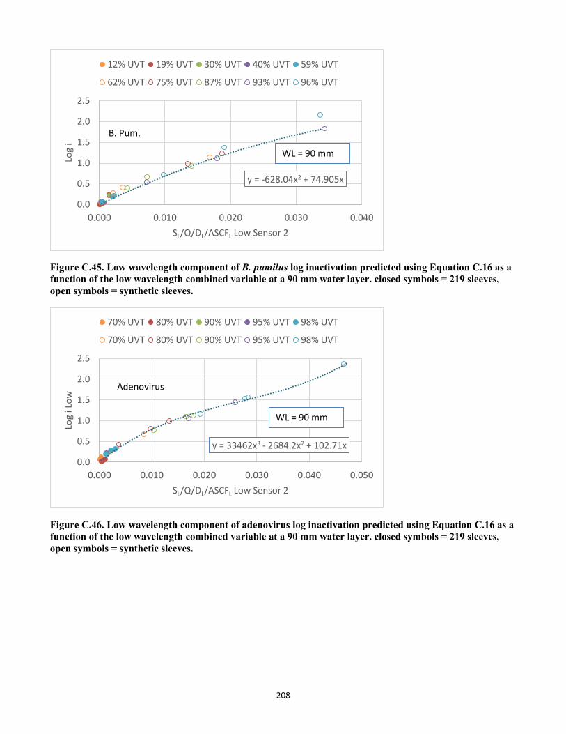
208

y = -628.04x2 + 74.905x

0.0

0.5

1.0

1.5

2.0

2.5

0.000 0.010 0.020 0.030 0.040

Log

i




B. Pum.

WL = 90 mm

Figure C.45. Low wavelength component of B. pumilus log inactivation predicted using Equation C.16 as a function of the low wavelength combined variable at a 90 mm water layer. closed symbols = 219 sleeves, open symbols = synthetic sleeves.

y = 33462x3 - 2684.2x2 + 102.71x

0.0

0.5

1.0

1.5

2.0

2.5

0.000 0.010 0.020 0.030 0.040 0.050

Log

i Low




Adenovirus

WL = 90 mm

Figure C.46. Low wavelength component of adenovirus log inactivation predicted using Equation C.16 as a function of the low wavelength combined variable at a 90 mm water layer. closed symbols = 219 sleeves, open symbols = synthetic sleeves.

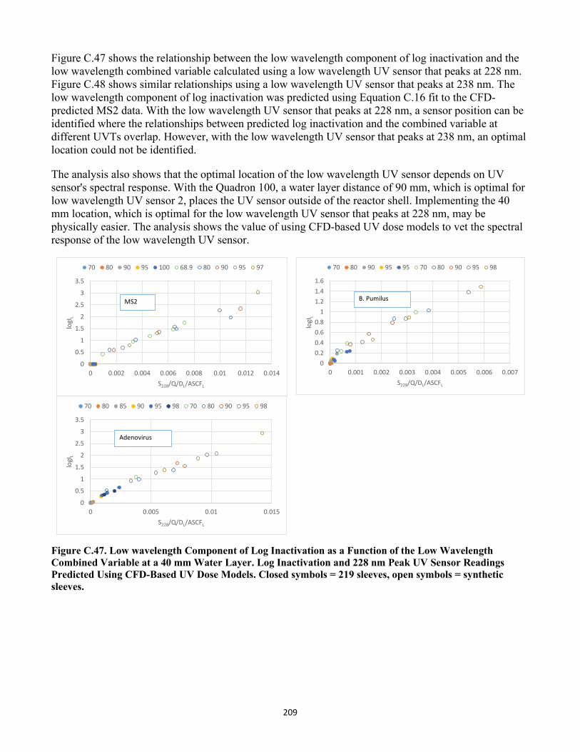
209

Figure C.47 shows the relationship between the low wavelength component of log inactivation and the low wavelength combined variable calculated using a low wavelength UV sensor that peaks at 228 nm. Figure C.48 shows similar relationships using a low wavelength UV sensor that peaks at 238 nm. The low wavelength component of log inactivation was predicted using Equation C.16 fit to the CFD-predicted MS2 data. With the low wavelength UV sensor that peaks at 228 nm, a sensor position can be identified where the relationships between predicted log inactivation and the combined variable at different UVTs overlap. However, with the low wavelength UV sensor that peaks at 238 nm, an optimal location could not be identified.

The analysis also shows that the optimal location of the low wavelength UV sensor depends on UV sensor's spectral response. With the Quadron 100, a water layer distance of 90 mm, which is optimal for low wavelength UV sensor 2, places the UV sensor outside of the reactor shell. Implementing the 40 mm location, which is optimal for the low wavelength UV sensor that peaks at 228 nm, may be physically easier. The analysis shows the value of using CFD-based UV dose models to vet the spectral response of the low wavelength UV sensor.

0

0.5

1

1.5

2

2.5

3

3.5

0 0.002 0.004 0.006 0.008 0.01 0.012 0.014

logI

L

S228/Q/DL/ASCFL

70 80 90 95 100 68.9 80 90 95 97

MS2

00.20.40.60.8

11.21.41.6

0 0.001 0.002 0.003 0.004 0.005 0.006 0.007

logI

L

S228/Q/DL/ASCFL

70 80 90 95 95 70 80 90 95 98

B. Pumilus

0

0.5

1

1.5

2

2.5

3

3.5

0 0.005 0.01 0.015

logI

L

S228/Q/DL/ASCFL

70 80 85 90 95 98 70 80 90 95 98

Adenovirus

Figure C.47. Low wavelength Component of Log Inactivation as a Function of the Low Wavelength Combined Variable at a 40 mm Water Layer. Log Inactivation and 228 nm Peak UV Sensor Readings Predicted Using CFD-Based UV Dose Models. Closed symbols = 219 sleeves, open symbols = synthetic sleeves.

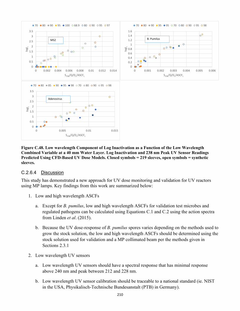
210

0

0.5

1

1.5

2

2.5

3

3.5

0 0.002 0.004 0.006 0.008 0.01 0.012 0.014

logI

L

S238/Q/DL/ASCFL

70 80 90 95 100 68.9 80 90 95 97

MS2

00.20.40.60.8

11.21.41.6

0 0.001 0.002 0.003 0.004 0.005 0.006

logI

L

S238/Q/DL/ASCFL

70 80 90 95 95 70 80 90 95 98

B. Pumilus

0

0.5

1

1.5

2

2.5

3

3.5

0 0.005 0.01 0.015

logI

L

S238/Q/DL/ASCFL

70 80 85 90 95 98 70 80 90 95 98

Adenovirus

Figure C.48. Low wavelength Component of Log Inactivation as a Function of the Low Wavelength Combined Variable at a 40 mm Water Layer. Log Inactivation and 238 nm Peak UV Sensor Readings Predicted Using CFD-Based UV Dose Models. Closed symbols = 219 sleeves, open symbols = synthetic sleeves.

C.2.6.4 Discussion This study has demonstrated a new approach for UV dose monitoring and validation for UV reactors using MP lamps. Key findings from this work are summarized below:

1. Low and high wavelength ASCFs

a. Except for B. pumilus, low and high wavelength ASCFs for validation test microbes and regulated pathogens can be calculated using Equations C.1 and C.2 using the action spectra from Linden et al. (2015).

b. Because the UV dose-response of B. pumilus spores varies depending on the methods used to grow the stock solution, the low and high wavelength ASCFs should be determined using the stock solution used for validation and a MP collimated beam per the methods given in Sections 2.3.1

2. Low wavelength UV sensors

a. Low wavelength UV sensors should have a spectral response that has minimal response above 240 nm and peak between 212 and 228 nm.

b. Low wavelength UV sensor calibration should be traceable to a national standard (ie. NIST in the USA, Physikalisch-Technische Bundesanstalt (PTB) in Germany).

https://www.ptb.de/cms/en.html

211

c. The UV system manufacturer should document the properties of the low wavelength UV sensors including spectral response from 200 to 400 nm, angular response, linearity over the working range, and temperature sensitivity from 0 to 30ºC.

d. As shown in this work, the spectral response of low wavelength UV sensors may not provide accurate monitoring if the UV sensor has response above 240 nm due to the primary or secondary peaks, or the UV sensor peaks at too low of a wavelength. As such, UV system manufacturers should use CFD-based UV dose models to vet their low wavelength UV sensors, showing that the spectral response is appropriate for the UV dose monitoring using the approaches described in this document.

e. During validation and operation of the UV reactor at the WTP, the low wavelength UV sensor readings should be set to zero if the UV sensor non-linearity deviates by more than 10 percent from a one-to-one relationship or the contribution of wavelengths above 240 nm due to the primary or secondary peaks is greater than 10 percent of the UV sensor reading.

f. During operation at the WTP, calibrated reference sensors should be used to check the accuracy of the low wavelength UV sensor. In keeping with the recommendations of the UVDGM, the duty UV sensor should read within 20 percent of the reference UV sensor.

3. Calculated dose equation using low and high wavelength UV sensors and ASCFs

a. Equation C.16 provides an algorithm for UV dose monitoring using low and high wavelength UV sensors and ASCF values

b. Equation C.16 can be fitted to data measured using multiple challenge microorganisms if ASCF values are used to normalize the data measured for different microbes to values expected using the action spectra of MS2.

c. Equation C.16 can be used to directly predict the log inactivation and RED expected with Cryptosporidium, Giardia, and adenovirus by setting the value of the UV dose per log inactivation (DL) to that of the pathogen based on the UV dose requirements of the LT2ESWTR and using low and high wavelength ASCF values specific to the pathogen.

d. Typically, validation conducted using MS2 and T1UV has low experimental noise resulting in equations that have a high R-squared (> 0.95). In contrast, with this work, validation conducted using B. pumilus spores had significant experimental noise. As such, it is recommended that Equation C.16 be fitted using validation collected using a combination of MS2 and T1UV phage. The equation can then be used to predict the log inactivation of pathogens provided that the low and high wavelength components of log inactivation lie within the validated range defined as a function of the low and high wavelength combined variables, respectively.

212

e. Validation data measured with MS2 and T1UV can be used to validate the UV dose monitoring equations by showing that an equation fitted to MS2 predicts T1UV and vice versa. This analysis provides confidence in the robustness of the individual datasets and verification that equations that use a combined variable can predict pathogen log inactivation using the UV sensitivity, DL, of that pathogen.

f. While the UVDGM recommends using multiple microbes to "bracket" the UV dose-response of the target pathogen, bracketing the UV dose-response of adenovirus using MS2 and B. pumilus spores did not improve the ability of Equation C.16 to predict adenovirus as opposed to using MS2 alone.

g. The validation test matrix should be designed to characterize the log inactivation at a given UVT at 254 nm as a function of the high wavelength combined variable using at least four points evenly spaced in terms of log inactivation. The UVTs at 254 nm should include the minimum and maximum UVTs plus intermediate UVTs that follow the geometric order:

𝑈𝑈𝑉𝑉𝐴𝐴𝑛𝑛 = 𝑈𝑈𝑉𝑉𝐴𝐴𝑀𝑀𝑀𝑀𝑛𝑛 × 𝛽𝛽𝑛𝑛−1 Equation C.24

where β is a constant with a recommended value between 2 and 2.5. For example, a UV reactor validated from 70 to 98 percent UVT would be tested at UVTs of 98, 95, 90, 79, and 70 percent.

h. The test matrix should include test conditions that maximize and minimize the contribution of low wavelengths. UV dose delivery can be maximized using synthetic quartz sleeves, source waters that have low absorbance below 240 nm, and Super Hume as a UV absorber. UV dose delivery can be minimized using Type 219 quartz sleeves (or equivalent), source water that have relatively high absorbance below 240 nm compared to 254 nm, and LSA as a UV absorber. The tests matrix should also include test conditions that provide an intermediate contribution of low wavelength dose delivery, such as synthetic sleeves with a source water that has high relative UV absorbance below 240 nm.

4. Calculated dose equation not using a UVT monitor

a. Equation C.21 provides a calculated UV dose approach that does not use online UVT monitors

b. Like the UV sensor setpoint approach as described in the UVDGM, the location of the low and high wavelength UV sensors, defined as the water layer distance between the UV sensor port window and the UV lamp, can be optimized to provide efficient UV dose monitoring. The optimization involves evaluating the relationship between the predicted low and high wavelength log inactivation predicted by Equation C.16 as a function of the low and high wavelength combined variables used by Equation C.21, respectively. At the optimal location, the relationship at different UVTs will tend to lie on top of each other when the log inactivation is plotted as a function of the combined variable. If the relationships at the optimal location do not exactly match, the relationship that predicts the lowest log inactivation value at a given value of the combined variable should be used to define monitoring. Those values can be used to conservatively define a relationship between the log

213

inactivation and the combined variable. The UV sensor location should be selected such that the relationship is defined by intermediate UVTs as opposed to the minimum or maximum UVT.

c. The optimal UV sensor location should be defined using relationship between log I and the combined variable measured using at least 4 values of UVT at 254 nm. The optimal location for the low wavelength UV sensor will depend on the UV sensor's spectral response and will likely differ from the optimal location for the high wavelength UV sensor.

214

Offal Business Office of Research and Development (8101R) Washington, DC 20460

Penalty for Private Use $300

Documents

Innovative Approaches for Validation of Ultraviolet