Embed Size (px)
Citation preview
Initiation of Streamers from Thundercloud
Hydrometeors
and Implications to Lightning Initiation
by
Samaneh Sadighi
Bachelor of Sciencein Physics
Sharif University of Technology2006
Master of Sciencein Physics
University of New Brunswick2009
A dissertationsubmitted to the College of Science at
Florida Institute of Technologyin partial fulfillment of the requirements
for the degree of
Doctor of Philosophyin
PhysicsMelbourne, Florida
May 2015

c© Copyright 2015 Samaneh SadighiAll Rights Reserved
The author grants permission to make single copies
We the undersigned committee hereby recommendthat the attached document be accepted as fulfilling in
part the requirements for the degree ofDoctor of Philosophy in Physics.
“Initiation of Streamers from Thundercloud Hydrometeors and Implications toLightning Initiation”,
a dissertation by Samaneh Sadighi
Dissertation AdvisorNingyu Liu, Ph.D.Associate Professor, Physics and Space Sciences
Dissertation Co-AdvisorHamid K. Rassoul, Ph.D.Professor, Physics and Space SciencesDean, College of Science
Joseph R. Dwyer, Ph.D.Professor, Physics, University of New HampshirePeter T. Paul Chair in Space Sciences
Ming Zhang, Ph.D.Professor, Physics and Space Sciences
Steven M. Lazarus, Ph.D.Professor, Marine and Environmental Systems
Abstract
TITLE: Initiation of Streamers from Thundercloud Hydrome-
teors and Implications to Lightning Initiation
AUTHOR: Samaneh Sadighi
MAJOR ADVISORS: Ningyu Liu, Ph.D. and Hamid K. Rassoul, Ph.D.
Electric field values measured inside thunderclouds have consistently been
reported to be up to an order of magnitude lower than the value required for
the conventional electrical breakdown of air. This result has made it difficult
to explain how lightning frequently occurs in thunderclouds. One theory that
has been offered to explain the lightning initiation process is the theory of
lightning initiation from hydrometeors. According to this theory, lightning can
be initiated from electrical discharges originating around thundercloud water or
ice particles in the measured thundercloud electric field. These particles, called
hydrometeors, can cause significant enhancement of the thundercloud electric
field in their vicinity, increasing the probability to initiate streamers that are
precursor discharges for the hot lightning leader channel.
For this dissertation research, we have focused our efforts on studying streamer
initiation and propagation from thundercloud hydrometeors. For the first part
of this study, we have further investigated the idea proposed by Liu et al. [2012b]
to study streamers from ionization column hydrometeors in thundercloud con-
ditions. We have performed simulations for ambient electric field values as low
as 0.3Ek at thundercloud altitudes. According to our results, initiation of stable
streamers from thundercloud hydrometeors in a 0.3Ek electric field is possible,
iii
only if enhanced ambient ionization levels are present ahead of the streamer.
We investigate the streamer branching behavior and characteristics, and test a
theory that has recently been proposed to explain this phenomenon [Savel’eva
et al., 2013].
In order to verify whether an ionization column is a proper representation of
a dielectric hydrometeor, for the second part of this dissertation we modify our
streamer discharge model to accommodate an isolated dielectric particle repre-
senting the hydrometeor inside the computational region. The development of
this model has enabled us to accurately simulate the discharges around dielec-
tric hydrometeors with various shapes and physical states. Streamer discharge
results obtained from the dielectric hydrometeor have been presented and com-
pared with the results obtained from the first part of this work. We compare
our modeling results with laboratory experiments and realistic thundercloud
conditions and discuss the implications of this study to lightning initiation and
other lightning related phenomena.
iv
Contents
Abstract iii
List of Figures x
List of Tables 1
1 Introduction 2
1.1 Lightning Phenomenology . . . . . . . . . . . . . . . . . . . . . 2
1.1.1 Thundercloud Charge Structure . . . . . . . . . . . . . . 4
1.1.2 Hydrometeor Terminology . . . . . . . . . . . . . . . . . 5
1.1.3 Cloud Electrification . . . . . . . . . . . . . . . . . . . . 7
1.1.4 Electric Field Measurements Inside Thunderclouds . . . 8
1.1.5 Electric Fields Observed Near Lightning Initiations . . . 10
1.1.6 Lightning Initiation Altitudes . . . . . . . . . . . . . . . 11
1.2 Electrical Discharge Processes in Air . . . . . . . . . . . . . . . 13
1.2.1 Electron Avalanche . . . . . . . . . . . . . . . . . . . . . 14
1.2.2 Streamer Discharges . . . . . . . . . . . . . . . . . . . . 15
1.2.3 Corona Discharges . . . . . . . . . . . . . . . . . . . . . 17
1.2.4 Leader Discharges . . . . . . . . . . . . . . . . . . . . . . 18
1.3 Lightning Initiation . . . . . . . . . . . . . . . . . . . . . . . . . 19
1.3.1 Conventional Breakdown Theory . . . . . . . . . . . . . 19
1.3.2 Runaway Breakdown Theory . . . . . . . . . . . . . . . . 20
1.4 Scientific Contributions . . . . . . . . . . . . . . . . . . . . . . . 21
2 Overview of Previous Experimental and Modeling Studies 24
2.1 Laboratory Experiments on Streamers from Hydrometeors . . . 25
2.1.1 Collision Between Water Drops . . . . . . . . . . . . . . 25
v
2.1.2 Ice Particles . . . . . . . . . . . . . . . . . . . . . . . . . 26
2.2 Theoretical Studies on Streamers from Hydrometeors . . . . . . 30
2.3 Streamer Discharge Model . . . . . . . . . . . . . . . . . . . . . 33
3 Streamers from Ionization Column Hydrometeors 36
3.1 Model Description . . . . . . . . . . . . . . . . . . . . . . . . . 36
3.2 Modeling Results for 0.5Ek . . . . . . . . . . . . . . . . . . . . . 39
3.3 Modeling Results for 0.3Ek . . . . . . . . . . . . . . . . . . . . . 40
3.4 Effects of Hydrometeor Dimension . . . . . . . . . . . . . . . . . 44
3.5 Effects of Ambient Density . . . . . . . . . . . . . . . . . . . . . 46
3.6 Streamer Branching and Head Curvature Analysis . . . . . . . . 53
3.7 Comparison with Realistic Hydrometeors . . . . . . . . . . . . . 63
3.8 Comparison with Laboratory Experiments . . . . . . . . . . . . 65
3.9 Role of Corona Discharges . . . . . . . . . . . . . . . . . . . . . 69
3.10 Role of Electron Detachment . . . . . . . . . . . . . . . . . . . . 72
3.11 Negative Streamers . . . . . . . . . . . . . . . . . . . . . . . . . 73
4 Streamers from Dielectric Hydrometeors 75
4.1 Dielectric Hydrometeor . . . . . . . . . . . . . . . . . . . . . . . 75
4.2 Model Description . . . . . . . . . . . . . . . . . . . . . . . . . 76
4.3 Cut-Cell Method for Resolving the Curved Boundary . . . . . . 78
4.4 Surface Area and Volume of the Cut Cells . . . . . . . . . . . . 80
4.5 Continuity Equation Solution Around the Curved Boundary . . 84
4.5.1 Particle Flux Calculation and Boundary Conditions . . . 85
4.6 Electric Field Calculation Around the
Curved Boundary . . . . . . . . . . . . . . . . . . . . . . . . . . 87
4.6.1 Contant Polarization: Solid Ice Particles . . . . . . . . . 88
4.6.2 Variable Polarization: Liquid Water Filaments . . . . . . 90
4.7 Modeling Results from the Dielectric Hydrometeor . . . . . . . . 95
4.7.1 Solid Ice Particles . . . . . . . . . . . . . . . . . . . . . . 95
4.7.2 Liquid Water Filaments . . . . . . . . . . . . . . . . . . 101
5 Summary and Future Work 106
5.1 Summary of Results . . . . . . . . . . . . . . . . . . . . . . . . 106
vi

5.2 Implications to Lightning Initiation . . . . . . . . . . . . . . . . 108
5.3 Suggestions for Future Work . . . . . . . . . . . . . . . . . . . . 110
vii
List of Figures
1.1 Four types of cloud-to-ground lightning flashes . . . . . . . . . . 3
1.2 Thundercloud charge structure . . . . . . . . . . . . . . . . . . . 5
1.3 Graupel-ice mechanism of cloud electrification . . . . . . . . . . 8
1.4 Observed electric fields from 50 balloon soundings, as a function
of altitude . . . . . . . . . . . . . . . . . . . . . . . . . . . . . . 12
1.5 (a) A positive streamer at two consecutive moments of time, (b)
A negative streamer at two consecutive moments of time . . . . 16
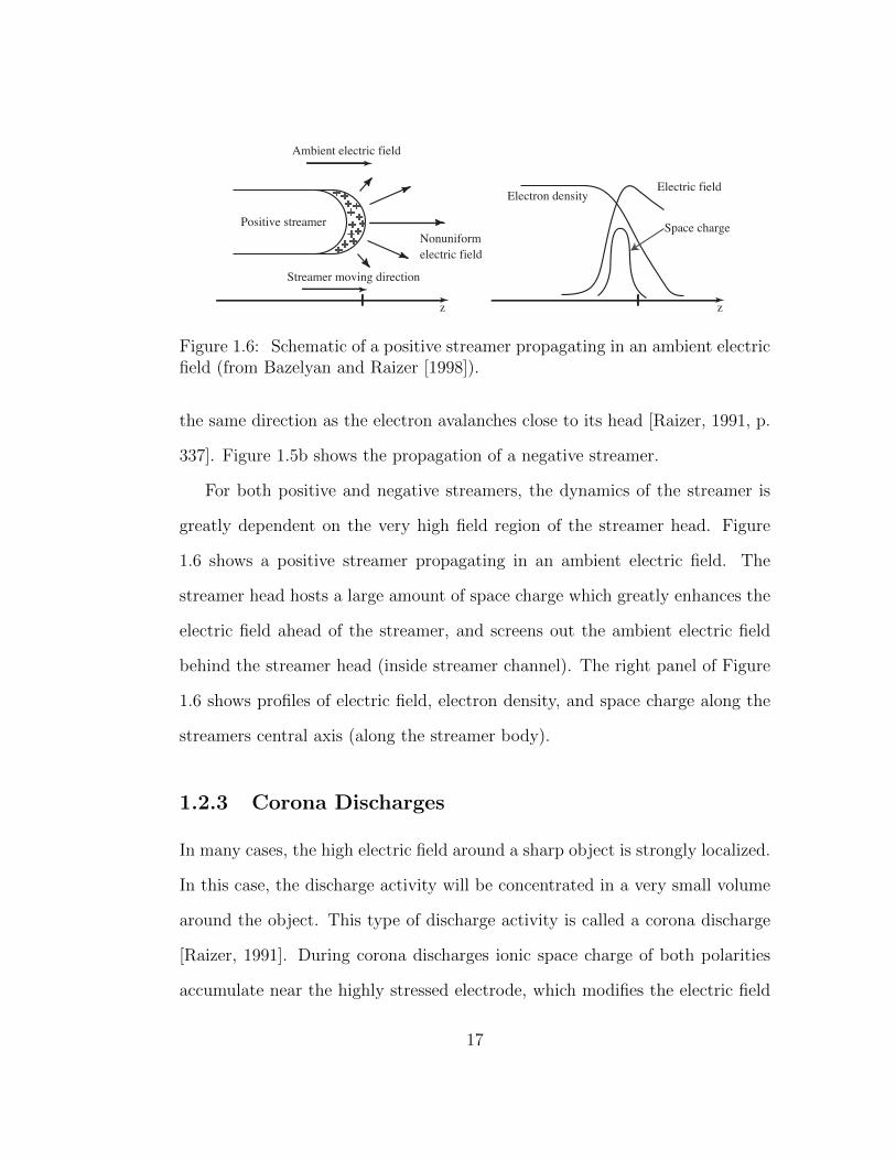
1.6 Schematic of a positive streamer propagating in an ambient elec-
tric field . . . . . . . . . . . . . . . . . . . . . . . . . . . . . . . 17
2.1 Schematic of the experimental setup of Crabb and Latham [1974]:
collision of two water drops . . . . . . . . . . . . . . . . . . . . 26
2.2 (a) Photograph of an ice needle cluster, (b) Photograph of a
positive streamer extending from the needle cluster . . . . . . . 28
2.3 (a) Photograph of a sample vapor-grown ice crystal habit, (b)
and (c) Photograph showing simultaneous continuous positive
and negative glow coronae formed at the tips of the ice crystal
extremities . . . . . . . . . . . . . . . . . . . . . . . . . . . . . . 29
2.4 Cross-sectional views of distributions of electron density and elec-
tric field of a streamer at ground pressure (Liu et al. [2012b]). . 34
3.1 Cross-sectional views of distributions of (a) electron density and
(b) electric field of a streamer from a hydrometeor in E0 = 0.5Ek
at 7 km altitude . . . . . . . . . . . . . . . . . . . . . . . . . . . 40
3.2 Cross-sectional views of distributions of (a) electron density and
(b) electric field of a streamer from a hydrometeor in E0 = 0.3Ek
at 7 km altitude . . . . . . . . . . . . . . . . . . . . . . . . . . . 41
viii
3.3 Time evolution of axial profiles of (a) electron density and (b)
electric field corresponding to the streamer in Figure 3.2 . . . . 43
3.4 Demonstration of the effect of the hydrometeor dimension on
streamer initiation . . . . . . . . . . . . . . . . . . . . . . . . . 45
3.5 Time evolution of axial profiles of electric field corresponding to
the streamer in Figure 3.4 . . . . . . . . . . . . . . . . . . . . . 48
3.6 Cross-sectional views of electron density distributions of (a) a
streamer that is about to branch, and (b, c) stable streamers,
from model hydrometeors . . . . . . . . . . . . . . . . . . . . . 50
3.7 Time evolution of the splitting of the streamer from Figure 3.6a 51
3.8 Axial profiles of (a) electric field and (b) electron density corre-
sponding to the streamers presented in Figure 3.6 . . . . . . . . 52
3.9 Images of streamer discharges in argon gas, exposed to laser ra-
diation . . . . . . . . . . . . . . . . . . . . . . . . . . . . . . . . 54
3.10 Electric field distribution on the surface of an ideal conductor in
the shape of a cylinder with a semielliptic head . . . . . . . . . 56
3.11 The streamer surface profiles corresponding to the cases in Figure
3.6 (a), (b), and (c), shown at a few different moments of time . 59
3.12 The electric field values on the streamer surfaces corresponding
to the same moments of time illustrated in Figure 3.11 . . . . . 61
3.13 The curvature of the surface of the streamer, corresponding to
the same moments of time illustrated in Figure 3.11 . . . . . . . 61
3.14 Sample photographs of discharges from ice hydrometeors . . . . 67
4.1 Geometry of the columniform dielectric hydrometeors used in this
study . . . . . . . . . . . . . . . . . . . . . . . . . . . . . . . . . 77
4.2 Cells that are cut by the curved boundary . . . . . . . . . . . . 79
4.3 The centers of the cells cut by the curved boundary . . . . . . . 81
4.4 Examples of reshaping of the cut cells . . . . . . . . . . . . . . . 82
4.5 (a) Different shapes of the cut cells, (b) Illustration of the surface
area produced due to the slanted side of the cut cell . . . . . . . 83
4.6 Schematic of reshaped boundary-cut cells . . . . . . . . . . . . . 86
4.7 Schematic illustration of the computational domain used for the
streamer simulation from spherical dielectric hydrometeors . . . 89
ix
4.8 Schematic illustration of the computational domain used for the
streamer simulation from columniform liquid dielectric hydrom-
eteors . . . . . . . . . . . . . . . . . . . . . . . . . . . . . . . . 92
4.9 Cross-sectional views of distributions of electron density (top)
and electric field (bottom) of a streamer formed from a spherical
dielectric hydrometeor (solid ice particle) . . . . . . . . . . . . . 96
4.10 Profiles of electron density (top) and electric field (bottom) along
the symmetry axis of the streamer in Figure 4.9 . . . . . . . . . 97
4.11 Profiles of electron density, electric field, and space charge density
along the symmetry axis of the streamer in Figure 4.9 . . . . . . 98
4.12 (top) Cross-sectional views of distributions of electron density
and electric field of streamers formed from two other setups with
the same dimension as the hydrometeor in Figure 4.9, (bottom)
Profiles of electron density, electric field, and charge density along
the symmetry axis for each streamer . . . . . . . . . . . . . . . 100
4.13 Cross-sectional views of distributions of electron density (top)
and electric field (bottom) of a streamer formed from a columni-
form dielectric hydrometeor (liquid water filament) . . . . . . . 102
4.14 Profiles of electron density (top) and electric field (bottom) along
the symmetry axis of the streamer in Figure 4.13 . . . . . . . . 103
4.15 Cross-sectional views of electron density and electric field of stream-
ers formed from: (top) a dielectric hydrometeor, and (bottom)
an ionization column hydrometeor . . . . . . . . . . . . . . . . . 104
x

List of Tables
1.1 Maximum electric field magnitudes measured in thunderclouds. 10
3.1 Streamer characteristics associated with the streamers from Fig-
ure 3.8. . . . . . . . . . . . . . . . . . . . . . . . . . . . . . . . . 53
3.2 List of different hydrometeor types and typical sizes . . . . . . . 64
4.1 Streamer characteristics measured for the three streamers in Fig-
ures 4.9 and 4.12, demonstrating the effects of different electrodes
on the streamer. . . . . . . . . . . . . . . . . . . . . . . . . . . . 99
1
Chapter 1
Introduction
1.1 Lightning Phenomenology
Lightning is a large electrical discharge that occurs in the atmosphere of the
Earth as well as other planets and can have a length of tens of kilometers or
more. More than 25% of the global lightning activity constitutes of cloud-to-
ground discharges. The remaining 75% is called cloud discharges and does not
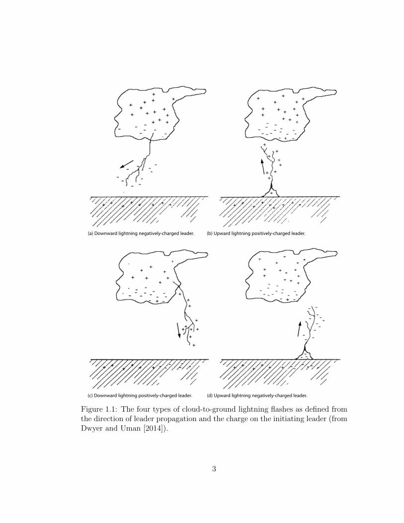
involve the ground. Depending on the polarity of the effective charge being
transported downward and the direction of propagation of the developing dis-
charge, four different types of cloud-to-ground lightning have been identified.
These include negative downward, positive downward, negative upward, and
positive upward discharges. More than 90% of cloud-to-ground discharges are
negative downward discharges [Rakov and Uman, 2003]. Figure 1.1 shows each
of these discharge types.
The primary source of lightning is the cumulonimbus, more commonly known
as the thundercloud. Thunderclouds can be thought of as large atmospheric heat
2
(a) Downward lightning negatively-charged leader. (b) Upward lightning positively-charged leader.
(c) Downward lightning positively-charged leader. (d) Upward lightning negatively-charged leader.
Figure 1.1: The four types of cloud-to-ground lightning flashes as defined fromthe direction of leader propagation and the charge on the initiating leader (fromDwyer and Uman [2014]).
3
engines. Their input energy comes from the sun and water vapor is the primary
heat-transfer agent. The principle outputs of a thundercloud include (i) the
mechanical work of vertical and horizontal winds, (ii) outflow of condensation
in the form of rain and hail from the bottom of the cloud and of small ice crystals
from the top of the cloud, and (iii) electrical discharges occurring inside, below
and above the cloud [Rakov and Uman, 2003].
1.1.1 Thundercloud Charge Structure
Wilson [1925] suggested that thunderclouds typically have positive charge above
negative charge in a positive dipole type of configuration. After Wilson, the gen-
erally accepted thundercloud charge structure was considered as three vertically
stacked regions: main positive at the top, main negative in the middle, and a
lower positive region at the bottom which may not always be present. The
dominant positive charge in the upper part of the thundercloud causes a layer
of charge of the opposite polarity to form on the upper cloud boundary. This
is called the screening charge layer. It is thought that in any region of the
thundercloud, charges of both polarity coexist, regardless of the polarity of the
net charge in that region [MacGorman and Rust, 1998]. A sketch depicting the
charge structure of the thundercloud is shown in Figure 1.2.
The magnitudes of the main positive and main negative charge regions are
typically a few tens of coulombs, while the lower positive charge region is about
ten coulombs or less. By approximating these charge regions as point charges,
the electric field intensity due to the system of three charges can be found by
replacing the perfectly conducting ground with three image charges [Rakov and
Uman, 2003].
4
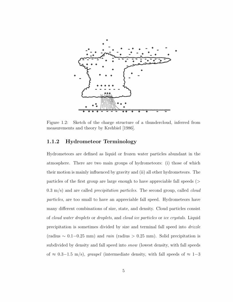
Figure 1.2: Sketch of the charge structure of a thundercloud, inferred frommeasurements and theory by Krehbiel [1986].
1.1.2 Hydrometeor Terminology
Hydrometeors are defined as liquid or frozen water particles abundant in the
atmosphere. There are two main groups of hydrometeors: (i) those of which
their motion is mainly influenced by gravity and (ii) all other hydrometeors. The
particles of the first group are large enough to have appreciable fall speeds (>
0.3 m/s) and are called precipitation particles. The second group, called cloud
particles, are too small to have an appreciable fall speed. Hydrometeors have
many different combinations of size, state, and density. Cloud particles consist
of cloud water droplets or droplets, and cloud ice particles or ice crystals. Liquid
precipitation is sometimes divided by size and terminal fall speed into drizzle
(radius ∼ 0.1−0.25 mm) and rain (radius > 0.25 mm). Solid precipitation is
subdivided by density and fall speed into snow (lowest density, with fall speeds
of ≈ 0.3−1.5 m/s), graupel (intermediate density, with fall speeds of ≈ 1−3
5
m/s), and hail (greatest density and possibly larger in size, with fall speeds up
to 50 m/s) [MacGorman and Rust, 1998].
There is no clear-cut size boundary between cloud and precipitation parti-
cles. Smaller particles are loosely called “cloud particles” and larger particles are
called “precipitation particles”, without specifying a definite size. Nevertheless,
we can still speak of typical sizes for these particles. Usually the following six
types of particles are distinguished in clouds [Wang, 2013]. The sizes indicate
the radius of the particle, unless otherwise noted:
• Cloud drops - water drops that are suspended in the cloud. Their typical
size range is from a few micrometers to ∼ 500 µm.
• Raindrops - water drops that are falling and may eventually reach the
ground. Typical size range is from a few hundred micrometers to ∼ 3
mm. Drizzle drops are a subcategory of raindrops with radius smaller
than 250 µm.
• Ice crystals - these refer to clean crystalline ice particles that are predom-
inantly of the hexagonal shape. However, needle or long solid column
shapes are also frequent. Their typical sizes range from a few tens of
micrometers to a few hundred micrometers.
• Snowflakes - crystalline ice particles of relatively large size. Their typical
size ranges are from a few hundred micrometers to a few centimeters.
• Graupel - when ice or snow crystals collide with supercooled water drops,
eventually a particle is produced called graupel. Graupel is considered the
6
precursor of hail. By convention, graupel particles must be smaller than
5 mm in diameter. If it grows greater than that it will be called hail.
• Hail - hailstones are the largest particles in a precipitation system. They
should be larger than 5 mm in diameter but can reach up to 15 cm.
1.1.3 Cloud Electrification
Determining how thunderclouds are electrified has been the goal of many ex-
periments and field observations for decades, during which many different cloud
electrification theories have been proposed [e.g., Wilson, 1929, Chiu and Klett,
1976, Takahashi, 1978]. Any cloud electrification mechanism must involve two
components: a small-scale process that electrifies individual hydrometeors, and
a process that spatially separates these charged hydrometeors, resulting in dis-
tances between cloud charge regions on the order of kilometers [Rakov and
Uman, 2003].
Here we will briefly overview one of the more popular cloud electrification
mechanisms, the noninductive graupel-ice mechanism. “Noninductive” refers to
any mechanism that does not require polarization of the hydrometeors by an
electric field. In this mechanism, electric charges are produced by collisions be-
tween graupel particles and ice crystals in the presence of water droplets, and
the large-scale separation of the charged particles is due to the action of gravity.
The existence of water droplets is necessary for significant charge transfer, as
demonstrated by laboratory experiments [Reynolds, 1953]. When heavy graupel
particles fall through a suspension of small ice crystals and supercooled water
drops, they can acquire negative or positive charges in collision with ice crys-
7
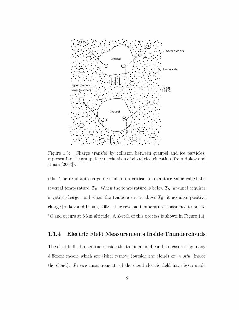
Figure 1.3: Charge transfer by collision between graupel and ice particles,representing the graupel-ice mechanism of cloud electrification (from Rakov andUman [2003]).
tals. The resultant charge depends on a critical temperature value called the
reversal temperature, TR. When the temperature is below TR, graupel acquires
negative charge, and when the temperature is above TR, it acquires positive
charge [Rakov and Uman, 2003]. The reversal temperature is assumed to be -15
◦C and occurs at 6 km altitude. A sketch of this process is shown in Figure 1.3.
1.1.4 Electric Field Measurements Inside Thunderclouds
The electric field magnitude inside the thundercloud can be measured by many
different means which are either remote (outside the cloud) or in situ (inside
the cloud). In situ measurements of the cloud electric field have been made
8
using (i) balloons carrying corona probes, (ii) balloons carrying electric field
meters, (iii) aircraft, (iv) rockets, and (v) parachuted electric field mills [Rakov
and Uman, 2003].
However, measuring the electric field inside a thundercloud is a very difficult
task for several reasons: (1) Thunderstorms are a large and violent environment,
which makes it challenging to make in situ measurements. (2) The thunderstorm
fields often change rapidly, on the time scale of seconds, and so even a jet aircraft
will only sample a small part of the cloud before the field changes. (3) Finally,
some lightning initiation models postulate that lightning forms from small water
droplets or ice. Placing a large (sometimes wet) object, such as balloon, aircraft
or rocket, could artificially discharge the thundercloud before the field has a
chance to build up to the point where lightning might be naturally initiated.
In other words, the act of observing the system may substantially perturb it
[Dwyer and Uman, 2014].
Much research dedicated to measuring thundercloud electric fields can be
found in the literature [e.g., Winn and Moore, 1971, Winn et al., 1974, Marshall
and Winn, 1982, Marshall and Rust, 1993, Stolzenburg et al., 1998a, Stolzen-
burg et al., 2007]. Many electric field measurements from inside active storms
show electric field magnitudes that are typically less than 150 kV/m [e.g., Mar-
shall and Rust, 1991], with a few extreme values of up to 1000 kV/m [e.g.,
Winn et al., 1981]. The maximum electric field magnitudes measured inside the
cloud have significant importance in understanding the processes that govern
lightning initiation. Table 1.1 summarizes the reported maximum electric field
magnitudes measured inside thunderclouds.
9
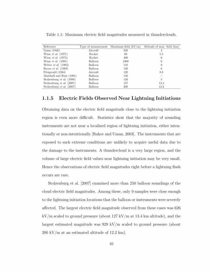
Table 1.1: Maximum electric field magnitudes measured in thunderclouds.
Reference Type of measurement Maximum field (kV/m) Altitude of max. field (km)Gunn (1948) Aircraft 340 4Winn et al. (1971) Rocket 60 5.5Winn et al. (1974) Rocket 400 6Winn et al. (1981) Balloon 1000 6Weber et al. (1982) Balloon 110 8Byrne et al. (1983) Balloon 130 8Fitzgerald (1984) Aircraft 120 8.8Marshall and Rust (1991) Balloon 146 −Stolzenburg et al. (1998) Balloon 120 5Stolzenburg et al. (2007) Balloon 127 13.4Stolzenburg et al. (2007) Balloon 200 12.2
1.1.5 Electric Fields Observed Near Lightning Initiations
Obtaining data on the electric field magnitude close to the lightning initiation
region is even more difficult. Statistics show that the majority of sounding
instruments are not near a localized region of lightning initiation, either inten-
tionally or non-intentionally [Rakov and Uman, 2003]. The instruments that are
exposed to such extreme conditions are unlikely to acquire useful data due to
the damage to the instruments. A thundercloud is a very large region, and the
volume of large electric field values near lightning initiation may be very small.
Hence the observations of electric field magnitudes right before a lightning flash
occurs are rare.
Stolzenburg et al. [2007] examined more than 250 balloon soundings of the
cloud electric field magnitudes. Among these, only 9 samples were close enough
to the lightning initiation locations that the balloon or instruments were severely
affected. The largest electric field magnitude observed from these cases was 626
kV/m scaled to ground pressure (about 127 kV/m at 13.4 km altitude), and the
largest estimated magnitude was 929 kV/m scaled to ground pressure (about
200 kV/m at an estimated altitude of 12.2 km).
10
1.1.6 Lightning Initiation Altitudes
The altitude of lightning initiation is one of the parameters that can be inferred
from electric field measurements. Using a vertical profile of the thundercloud
electric field, a one-dimensional approximation to Gauss’s law is sufficient to
carry out this analysis [Stolzenburg et al., 1998a]. This can be done because
the largest component of the electric field in a sounding is usually in the ver-
tical direction. Furthermore, electric potential as a function of altitude can be
estimated from electric field soundings by integrating upward from the ground
[Marshall et al., 2001].
Figure 1.4 shows observed electric field values from 50 different balloon mea-
surements, as a function of altitude. The figure shows the theoretical threshold
electric field for conventional and runaway breakdown processes (see two theo-
ries for lightning initiation, discussed in Section 1.3). The measurements in the
figure are for three different storm types, each corresponding to different color
marks. The circled values are extreme values associated with close lightning.
The two values enclosed by red boxes are at known distances of 1100−2100 m
from a subsequent lightning initiation location.
Figure 1.4 gives an indication of typical altitudes for lightning initiation.
The most likely electric field values to initiate lightning are the points closest
to the threshold curves. For the positive values, this altitude ranges between
4−6 km. This altitude range typically corresponds to the region between the
lower positive and main negative charge regions in the storm, making negative
cloud-to-ground lightning the most probable type of lightning to occur [e.g.,
Stolzenburg et al., 2003]. On the negative side of measured electric fields, the
peak values are observed between about 6−11 km, corresponding to the region
11
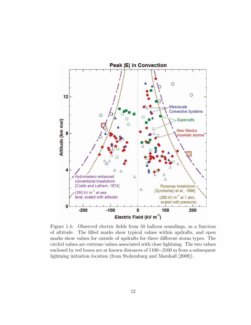
Figure 1.4: Observed electric fields from 50 balloon soundings, as a functionof altitude. The filled marks show typical values within updrafts, and openmarks show values for outside of updrafts for three different storm types. Thecircled values are extreme values associated with close lightning. The two valuesenclosed by red boxes are at known distances of 1100−2100 m from a subsequentlightning initiation location (from Stolzenburg and Marshall [2009]).
12
above the main negative charge layer [e.g., Marshall and Rust, 1991]. This
is the region that intra-cloud lightning flashes are more likely to occur [e.g.,
Stolzenburg et al., 1998b]. Generally, the altitude of lightning initiation greatly
depends on the type of the thunderstorm, the charge structure of the cloud,
and the location of measurements [Rakov and Uman, 2003]. Different initiation
altitudes give rise to different types of lightning discharges [e.g., Krehbiel et al.,
2008].
1.2 Electrical Discharge Processes in Air
Air is generally a good insulator and can maintain it’s insulating properties until
the applied electric field exceeds about 3.2×10⁶ V/m at standard atmospheric
temperature and pressure. If the background electric field exceeds this critical
value, free electrons in air will gain enough energy to ionize other atoms and
molecules through collisions. This ionization leads to an increase in the number
of electrons, which initiates the electrical breakdown of air. This critical thresh-
old value is called the conventional breakdown threshold field of air (Ek) and is
defined as the equality of the ionization and dissociative attachment coefficients
in air [Raizer, 1991, p.135]. Its value scales with atmospheric density, N, as
follows:
E = E0N
N0
, (1.1)
where E0 and N0 are the critical electric field and the density of air at standard
atmospheric conditions, respectively. The air density in the Earth’s atmosphere
decreases exponentially with height as N = N0e−z/H , with H ≈ 7 km being the
13
atmosphere scale height. So the critical electric field required to cause electrical
breakdown in the atmosphere will also decreases with height:
E = E0e−z/H . (1.2)
Different types of electrical discharges that occur in the atmosphere consist of
four basic processes, electron avalanches, streamer discharges, corona discharges,
and leaders. A brief description of each of these discharge types will be provided
below.
1.2.1 Electron Avalanche
An electron avalanche is the primary element of any breakdown mechanism.
Consider a free electron moving under the influence of a background electric
field. If the background field is larger than Ek, the electron may produce another
electron through ionization collisions. These two electrons will give rise to two
more electrons and this process continues [Cooray, 2012, p.68]. Let α be the
number of ionizing collisions per unit length, and η the number of electron
attachments per unit length. In traveling across a length of dx, ne0 number of
electrons will give rise to dn additional electrons:
dn = ne0(α− η)dx. (1.3)
This equation shows that the number of electrons will increase exponentially:
ne = ne0e(α−η)x. (1.4)
14
The exponential growth of the number of electrons with distance is called an
electron avalanche. The critical electric field beyond which air will electrically
breakdown is achieved when α = η. For electric fields below the breakdown
threshold, (α − η) < 0, and for fields higher than the threshold, (α − η) > 0
[Cooray, 2012, p.68].
1.2.2 Streamer Discharges
Streamers are narrow filamentary plasma discharge channels, which are the
precursors of the lightning leader [Rakov and Uman, 2003, p.137]. A streamer
is a weakly ionized thin channel formed from an avalanche in a sufficiently strong
electric field [Raizer, 1991, p. 334]. As an electron avalanche is moving forward,
the number of charged particles in the avalanche head is increasing. It has
been estimated that an avalanche will transition into a streamer if the number
of positive ions in the avalanche head reaches a value of about 108 [Loeb and
Meek, 1940] at ground pressure. Thus the condition for the transformation of
an avalanche to a streamer can be written as below [Cooray, 2012]:
exp(
∫ xc
0
[α(x)− η(x)]dx = 108 − 109, (1.5)
where x is the distance from the origin of the avalanche, and xc is the distance
from the origin of the avalanche to where the background field falls below Ek.
A streamer discharge is either positive or negative depending on the polarity
of the charge in its head. Each of these types has a different propagation
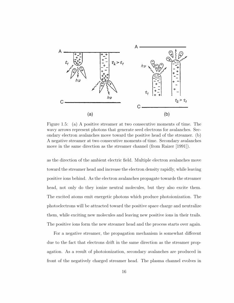
mechanism. The mechanism of propagation of a positive streamer is depicted
in Figure 1.5a. The propagation direction of the positive streamer is the same
15
A
CC
A
(a) (b)
Figure 1.5: (a) A positive streamer at two consecutive moments of time. Thewavy arrows represent photons that generate seed electrons for avalanches. Sec-ondary electron avalanches move toward the positive head of the streamer. (b)A negative streamer at two consecutive moments of time. Secondary avalanchesmove in the same direction as the streamer channel (from Raizer [1991]).
as the direction of the ambient electric field. Multiple electron avalanches move
toward the streamer head and increase the electron density rapidly, while leaving
positive ions behind. As the electron avalanches propagate towards the streamer
head, not only do they ionize neutral molecules, but they also excite them.
The excited atoms emit energetic photons which produce photoionization. The
photoelectrons will be attracted toward the positive space charge and neutralize
them, while exciting new molecules and leaving new positive ions in their trails.
The positive ions form the new streamer head and the process starts over again.
For a negative streamer, the propagation mechanism is somewhat different
due to the fact that electrons drift in the same direction as the streamer prop-
agation. As a result of photoionization, secondary avalanches are produced in
front of the negatively charged streamer head. The plasma channel evolves in
16
28
turb the electric field and are no longer independent, which leads to the streamer
mechanism of discharges. Streamer discharge theory was put forward in the 1930’s
to explain spark discharge [Loeb and Meek , 1940]. The theory is based on the con-
cept of a streamer. Streamers are narrow filamentary plasmas, which are driven
by highly nonlinear space charge waves [e.g., Raizer , 1991, p. 327]. The dynamics
of a streamer is mostly controlled by a highly enhanced field region, known as a
streamer head, and the streamer polarity is defined by the sign of the charge in its
head. A schematic illustration of a positive streamer propagating in an ambient
electric field is given in the left panel of Figure 2.2. The right panel of the figure
+
++++++
+++
++ +
Electron densityElectric field
Space chargePositive streamerNonuniformelectric field
Ambient electric field
Streamer moving direction
z z
Figure 2.2. Schematic of a positive streamer propagating in an ambient field (adaptedfrom [Bazelyan and Raizer , 1998, p. 45]).
gives the distribution of electron density, electric field and space charge along the
central axis of the streamer that is usually considered having cylindrical symmetry.
The propagation direction of the positive streamer is the same as the direction of
the ambient electric field. A large amount of space charges exists in the streamer
head (the shaded region in the figure), which strongly enhances the electric field
in the region just ahead of the streamer, while screening the ambient field out of
the streamer channel (the region behind of the streamer head). The peak space
charge field can reach a value about 4-7 times breakdown field Ek [e.g., Dhali and
Figure 1.6: Schematic of a positive streamer propagating in an ambient electricfield (from Bazelyan and Raizer [1998]).
the same direction as the electron avalanches close to its head [Raizer, 1991, p.
337]. Figure 1.5b shows the propagation of a negative streamer.
For both positive and negative streamers, the dynamics of the streamer is
greatly dependent on the very high field region of the streamer head. Figure
1.6 shows a positive streamer propagating in an ambient electric field. The
streamer head hosts a large amount of space charge which greatly enhances the
electric field ahead of the streamer, and screens out the ambient electric field
behind the streamer head (inside streamer channel). The right panel of Figure
1.6 shows profiles of electric field, electron density, and space charge along the
streamers central axis (along the streamer body).
1.2.3 Corona Discharges
In many cases, the high electric field around a sharp object is strongly localized.
In this case, the discharge activity will be concentrated in a very small volume
around the object. This type of discharge activity is called a corona discharge
[Raizer, 1991]. During corona discharges ionic space charge of both polarities
accumulate near the highly stressed electrode, which modifies the electric field
17
distribution. Similar to streamer discharges, corona discharges have positive
and negative polarity depending on the polarity of the electrode.
Corona discharges can occur from conductors in a variety of different loca-
tions and situations in the atmosphere. For example, corona can occur from
pointed objects connected to the ground, from cables and wires above the
ground, and in regions of high electric field magnitudes in thunderclouds from
rain and wet ice particles [e.g., Loeb, 1966]. The electrons emitted by corona
can form regions of space charge in the thundercloud and some of these sources
make a significant contribution to other forms of electrical discharges in the
atmosphere (see section 3.9 for more details).
1.2.4 Leader Discharges
A leader is a highly ionized, highly conductive channel that grows along the
path prepared by preceding streamers [Raizer, 1991]. Compared to a streamer,
a leader discharge is a hot discharge (∼ 5000−6000 K) and the conductivity of
its channel is very high. The leader head has strong electric field magnitudes.
Therefore, many streamers are sent out from the leader tip, and they draw a
large total current from it. The current heats the gas and creates a new head,
so the strongly ionized leader channel can advance [Raizer, 1991].
The most important condition necessary for leader formation is an increase
in gas temperature, leading to a sustained high channel conductivity. An indi-
vidual streamer is a cold discharge (about room temperature) and the current
associated with it cannot heat the air sufficiently to sustain its high conduc-
tivity in the channel. However, if the current from a group of streamers with
a common origin (called the streamer stem) is combined, the common channel
18
will heat up and the conductivity of the channel can be maintained [Cooray,
2012]. Thus, the current flow will be concentrated to a thin channel (i.e. the
streamer stem) and produce more heat and more ionization [Raizer, 1991]. With
increasing ionization, the process of transformation of the streamer stem into a
hot and conducting leader channel will take place.
1.3 Lightning Initiation
One of the important unanswered questions in atmospheric electricity is how
lightning is initiated inside thunderclouds. Despite the progress in the field of
atmospheric electricity in the recent decades, the specific mechanism and the
exact ambient electric field magnitude available for lightning initiation remain
unknown. Two theories have been proposed as the underlying mechanism of
lightning initiation; conventional and runaway breakdown. We will discuss them
in the following sections.
1.3.1 Conventional Breakdown Theory
One theory of air electrical breakdown that has been applied to explaining
the initiation of lightning discharges is the conventional breakdown theory [e.g.,
MacGorman and Rust, 1998, p.86, Rakov and Uman, 2003, p.121]. According to
this theory, in order for a lightning leader to form, the electric field value inside
some part of the cloud must exceed the conventional breakdown threshold field
of air. Despite the constant lightning activity observed in the atmosphere, years
of in situ measurements of the thundercloud electric fields have consistently
shown electric field values of well below the breakdown field. The maximum
19
values recorded in Table 1.1 are insufficient to initiate electron avalanches and
then the electrical breakdown process.
To overcome this obstacle, the theory of lightning initiation from thunder-
cloud hydrometeors (water drops, ice crystals, etc.) was brought forward [e.g.,
Dawson, 1969, Griffiths and Latham, 1974, Crabb and Latham, 1974]. Hy-
drometeors are abundant in the thundercloud environment (see section 1.1.2)
and when they are subject to an external electric field, they can cause significant
field enhancement in their vicinity. A critical component of the conventional
breakdown theory is to demonstrate that streamers are able to form and propa-
gate in an electric field magnitude similar to the observed thundercloud electric
fields. Investigation of this topic is the focus of this dissertation research.
1.3.2 Runaway Breakdown Theory
Another theory for lightning initiation is the runaway breakdown theory. Wilson
[1925] discovered the runaway electron mechanism in which fast electrons may
obtain large energies from static electric fields in air. When the rate of energy
gain from an electric field exceeds the rate of energy loss from interactions with
air then the energy of an electron will increase and it will “run away” [e.g, Dwyer,
2003, Dwyer et al., 2012]. The threshold electric field at which this happens is
about 2.8×10⁵ V/m and is scaled with air density. Gurevich et al. [1992] showed
that runaway electrons can undergo avalanche multiplication, resulting in a
large number of high energy runaway electrons. This avalanche mechanism is
commonly referred to as the Relativistic Runaway Electron Avalanche (RREA)
mechanism [Babich et al., 1998, Babich et al., 2001]. Gurevich and Zybin [2001]
hypothesized that the RREA mechanism can lead to the electrical breakdown
20
of air, which they called “runaway breakdown”.
The threshold electric field for runaway breakdown is an order of magnitude
less than the conventional breakdown threshold field. This fact has intrigued
many researchers to investigate the implications of this mechanism on lightning
initiation and lightning related phenomena [e.g., Dwyer, 2005, Dwyer, 2007,
Dwyer, 2010, Dwyer et al., 2012]. Although this theory offers an advantage over
the conventional breakdown theory, a lower threshold field, it has difficulty in
producing the spatially compact lightning channel and its high electron density.
Also, several authors have noted that runaway breakdown process itself may
discharge the large-scale electric fields inside thunderstorms, shutting down the
processes leading to lightning initiation [e.g., Gurevich et al., 1992, Marshall
et al., 1995, Solomon et al., 2001]. The RREA processes can at most provide
ambient conditions (e.g., producing a plasma domain) for the compact lightning
channels to develop [Babich et al., 2012].
1.4 Scientific Contributions
The occurrence of a lightning flash entails highly complicated processes. A com-
prehensive understanding of lightning requires understanding all the microphys-
ical processes involved in electrical breakdown, and the macroscale processes in
flash propagation that typically covers tens of kilometers of path length in a
single flash. For this dissertation, we investigate the initial stage of the light-
ning initiation process, by means of streamer emission from thundercloud hy-
drometeors, through theoretical and numerical modeling. The major scientific
contributions resulting from this dissertation work are summarized as follows:
21
1. We have developed a model capable of simulating streamers initiated from
isolated dielectric hydrometeors. This model is a modification of the sprite
streamer model by Liu and Pasko [2004]. It can be used to simulate
any dielectric hydrometeor shape with irregular curved boundaries. This
model allows studies of positive and negative streamers forming from a
hydrometeor, and analysis of the streamer and hydrometeor interactions.
2. We have established that streamers can be initiated from model hydrom-
eteors in maximum observed thundercloud electric fields. The lowest am-
bient electric field capable of initiating a streamer from realistic hydrom-
eteors at 7 km altitude is found to be 0.3Ek, where Ek is the conventional
breakdown threshold value.
3. Background ambient electron density existent inside the thundercloud has
been identified to promote the formation and propagation of stable stream-
ers. Depending on the magnitude and distribution, this density affects the
streamer formation stage, and can be a determining factor on whether the
streamer branches, recovers after the pre-branching stage, or continues
propagating stably.
4. Geometry of the streamer head has been determined to play an important
role in the streamer branching phenomenon. The fast radial movement of
the maximum streamer head curvature, combined with the slow reduction
of the maximum curvature value causes the streamer head to eventually
pull the maximum electric field off of the symmetry axis. The redistribu-
tion of the electric field profile with the maximum moving away from the
axis is a critical turning point for the streamer head. As the location of
22
the maximum electric field is also the fastest growth point of the streamer
head surface, this phenomenon results in the streamer propagating off-axis
and hence branching.
5. The dimension of the model hydrometeor has also been identified as a
critical parameter for streamer formation. The minimum length required
for the hydrometeor in order to initiate streamers in a 0.3Ek field has been
obtained to be between 5 and 8 mm, when a background ambient density
on the order of 1015 m−3 is included. The minimum length decreases
slightly with increasing background density. This range overlaps with the
range of lengths obtained from experimental studies on streamers from
hydrometeors.
23
Chapter 2
Overview of Previous
Experimental and Modeling
Studies
As described in Chapter 1, the conventional breakdown theory for lightning
initiation suggests that hydrometeors in the thundercloud locally enhance the
electric field to a value greater than the conventional breakdown threshold so
that the discharge process can be initiated. In this chapter, we will give a brief
overview of the laboratory experiments and theoretical studies that have been
dedicated to test this theory. Later in the chapter we will describe the numerical
model that we have used for the present work.
24
2.1 Laboratory Experiments on Streamers from
Hydrometeors
The majority of the experiments designed to investigate the conditions under
which streamer corona discharges may be produced have been conducted on two
main hydrometeor groups: water drops and ice crystals. Richards and Dawson
[1971] suggested that the collision of a pair of raindrops temporarily produces
an elongated filament of water, which provides a favorable site for the initiation
of streamers. The second group, ice crystals, have been used to examine the
conditions under which streamers can be initiated from their extremities. Blyth
et al. [1998] concluded that these two are the only two microphysical situations
that appear to be capable of initiating a discharge in the low thundercloud
electric fields. A summary of these experimental studies is presented below.
2.1.1 Collision Between Water Drops
Crabb and Latham [1974] measured the electric field values required to produce
streamer corona discharges from a pair of colliding water drops. According to
their experiments, a pair of raindrops colliding within a thundercloud produces
a deformed elongated object whose shape is particularly favorable for corona
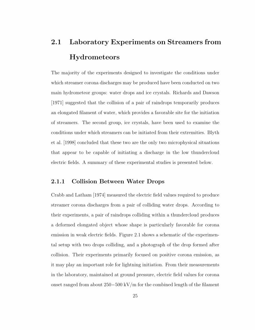
emission in weak electric fields. Figure 2.1 shows a schematic of the experimen-
tal setup with two drops colliding, and a photograph of the drop formed after
collision. Their experiments primarily focused on positive corona emission, as
it may play an important role for lightning initiation. From their measurements
in the laboratory, maintained at ground pressure, electric field values for corona
onset ranged from about 250−500 kV/m for the combined length of the filament
25
E
Large drop
R=2.7 mm
Small drop
r=0.65 mm
HV +
(a) (b)
Figure 2.1: (a) Schematic of the experimental setup of Crabb and Latham[1974], in which two drops with radii 2.7 mm and 0.65 mm collided in thepresence of an applied electric field. (b) Photograph of the elongated dropthat formed after collision (from Crabb and Latham [1974] and Schroeder et al.[1999]).
between 5−25 mm. They also confirmed the pattern of decreasing onset field
with the increasing combined length of the liquid filament suggested by Grif-
fiths and Latham [1974] for ice specimen. They concluded that the emission
of positive coronas from colliding raindrops can readily occur in thunderclouds
and therefore be a possible source for triggering lightning.
2.1.2 Ice Particles
Experimental studies conducted by Griffiths and Latham [1974] have shown that
positive streamers and various forms of corona discharges (e.g., steady glows,
Trichel pulses, breakdown streamers, and sparks) can be produced from ice hy-
drometeors a few millimeters in length suspended in a uniform electric field, for
temperatures above −18◦C. They studied many different types of ice specimen,
all showing that the currents obtained upon onset are sufficient to produce all
26
the mentioned types of discharges, including the continuous initiation of pos-
itive streamers. They suggested that hydrometeors with longer lengths can
produce streamer discharges easier than shorter lengths, due to higher polar-
ization charge and field enhancement at their tips. They concluded that the
role of streamer corona discharges from ice hydrometeors in a thunderstorm is
of great importance to lightning initiation, and the ambient fields necessary for
corona emission from ice in the central regions of thunderclouds are probably
in the range of 400−500 kV/m at ground pressure.
In further work, Griffiths [1975] examined the dependence of the electric field
required for corona onset on the electric charge carried by ice crystals. It was
found that the charges on the order of 10−10 C carried by the specimens reduced
the required electric field value by as much as 20%. Additionally, Griffiths and
Latham [1974] established that the temperature below which substantial corona
currents were inhibited due to surface conductivity reduction depended on the
purity of the ice sample. This value is reduced from −18◦C to −25◦C when the
surface of a pure sample was contaminated with a solution containing 4.5 mg
of ammonia per kilogram of water.
More recently, Petersen et al. [2006] conducted a series of laboratory experi-
ments on positive streamer emission from ice hydrometeors. The vertical dimen-
sions of the ice crystals ranged from 0.5−3 mm. Their results show that positive
streamer discharges are able to occur at temperatures as low as −38◦C when
subject to electric fields between 500−850 kV/m at ground pressure. This result
is in contrast with the finding by Griffiths and Latham [1974], which indicate
that positive streamers can only occur at temperatures greater than −18◦C for
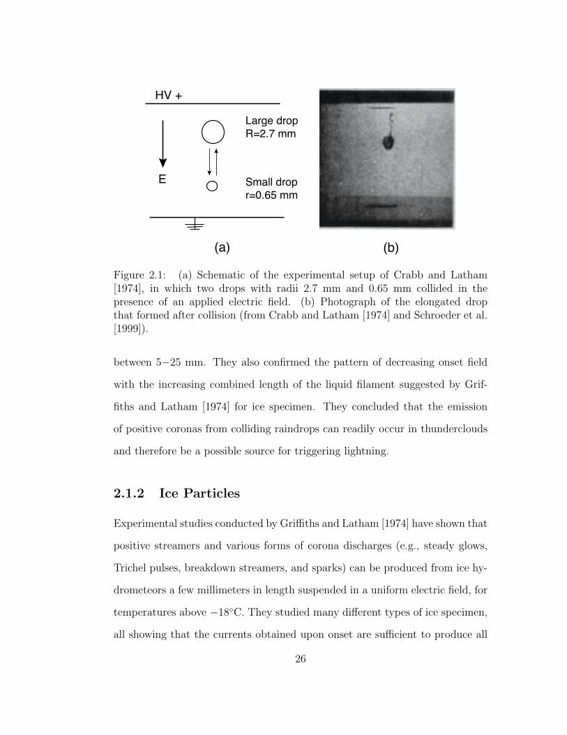
pure ice crystals. Figure 2.2 shows a sample photograph from their experiments;
27
b
Positive StreamersIce Crystal Needles
Glass
Filament
Figure 2.2: (a) Photograph showing a cluster of needles of approximately 2 mmvertical extent at the end of the glass thread. (b) Photograph of a luminoustrace of a positive streamer, extending from the needle cluster to the bottomelectrode (from Petersen et al. [2006]).
an ice crystal cluster and a positive streamer forming from it. They concluded
that the results from their experiments suggest that positive streamers from
frozen precipitation particles in the high altitude regions of the thundercloud
may occur and may in fact be a necessary element for the lightning initiation
process.
Petersen et al. [2014] extended their previous work by reporting a new labo-
ratory investigation on the initiation of streamer discharges from small ice crys-
tals. They observed different types of electrical discharges (glow corona, pulse
corona, and positive and negative streamers) from a variety of vapor-grown
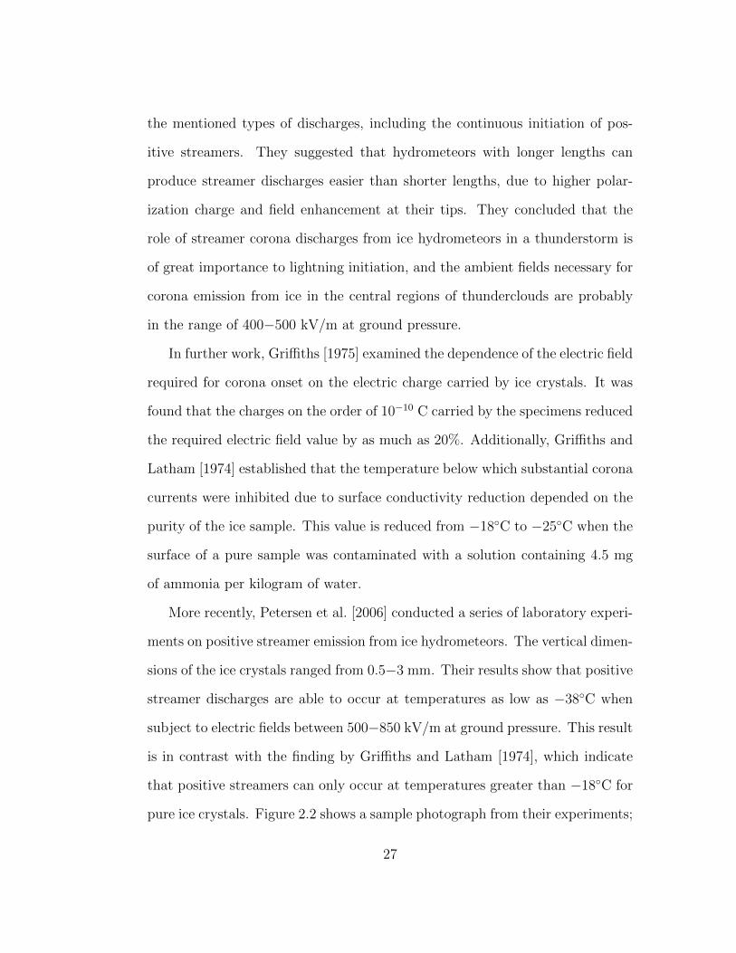
ice crystal shapes. Figure 2.3 shows a grown ice crystal habit and examples
of such discharges. The primary parameters that effect the threshold electric
field for positive streamer initiation were determined to be the length of the ice
crystal and air density. Observed threshold electric fields for positive streamers
at −14◦C and 570 mb pressure (about 5 km altitude) were between 700−2000
kV/m, for ice crystal lengths decreasing from 5 mm to 1 mm, larger than values
observed previously [e.g., Griffiths and Latham, 1974, Petersen et al., 2006]. The
28
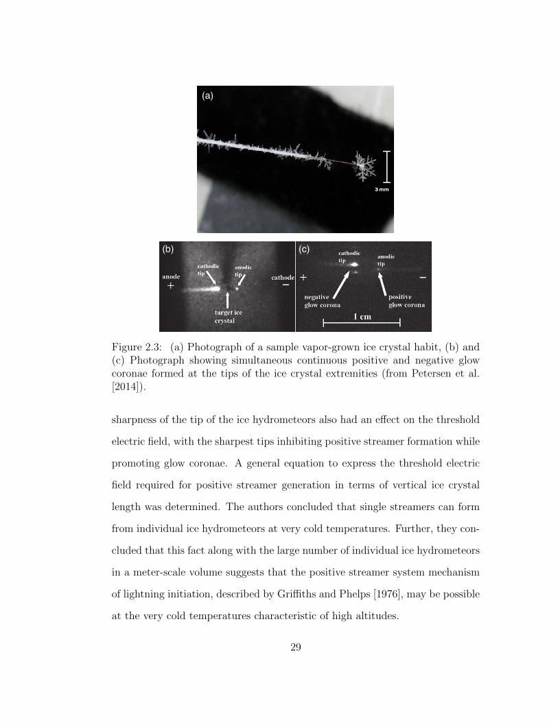
(a)
(c)(b)
Figure 2.3: (a) Photograph of a sample vapor-grown ice crystal habit, (b) and(c) Photograph showing simultaneous continuous positive and negative glowcoronae formed at the tips of the ice crystal extremities (from Petersen et al.[2014]).
sharpness of the tip of the ice hydrometeors also had an effect on the threshold
electric field, with the sharpest tips inhibiting positive streamer formation while
promoting glow coronae. A general equation to express the threshold electric
field required for positive streamer generation in terms of vertical ice crystal
length was determined. The authors concluded that single streamers can form
from individual ice hydrometeors at very cold temperatures. Further, they con-
cluded that this fact along with the large number of individual ice hydrometeors
in a meter-scale volume suggests that the positive streamer system mechanism
of lightning initiation, described by Griffiths and Phelps [1976], may be possible
at the very cold temperatures characteristic of high altitudes.
29
2.2 Theoretical Studies on Streamers from Hy-
drometeors
Phelps [1974] hypothesized that a single positive streamer, subjected to a strong
electric field, would rapidly intensify and branch. While this intensifying streamer
system propagates, it carries an increasing amount of positive charge in its tip,
and deposits negative charge in its trail. This charge distribution results in a
local dipole that enhances the electric field at the positive streamer origin. If a
series of these streamer systems were to propagate sequentially, each one advanc-
ing into the charge debris of its predecessors, the local electric field can intensify
up to the conventional breakdown threshold, implying that the resulting strong
electric field could support the emergence of a lightning leader.
Griffiths and Phelps [1976] used a numerical model to calculate the elec-
tric field enhancement in a thundercloud due to the propagation of a growing
system of positive streamers, similar to what was described in Phelps [1974].
Their model assumes that the streamer system propagates through a conical
volume in a series of steps. The positive charge in the head of the system is
assumed to be uniformly distributed on a circular disc, constituting the base of
the cone. The deposited negative charge is assumed to be located on a series
of discs, also uniformly charged, located halfway between each step. Supposing
the streamer system starts with an initial charge Q0, advancement of each pos-
itive disc is assumed to add ∆Q charge onto it. An amount of charge -∆Q will
be deposited uniformly on a disc halfway between the step, forming the next
negative disc. For the passage of the first streamer, the electric field is equal to
the chosen constant ambient field. However, in order to model subsequent pas-
30
sages of streamers into the deposited charge debris of the preceding streamers,
the field computed at each step must be a sum of the ambient field along with
the field due to the charge deposited by all previous streamer systems. The
authors conclude that the described model is capable of producing electric field
magnitudes as strong as the conventional breakdown, by the multiple passages
of streamer systems.
Schroeder et al. [1999] conducted a modeling study of positive streamer emis-
sion around a simulated coalesced water drop. They modeled positive discharges
using a one-dimensional drift-diffusion equation, paired with an analytical so-
lution to the electric field. They studied the positive streamer mechanism and
obtained results appearing to be consistent with the laboratory observations of
Crabb and Latham [1974]. Their results show that the minimum electric field re-
quired for a positive streamer to form from a pair of colliding water drops (drop
sizes similar to Crabb and Latham [1974]) is 500 kV/m at ground pressure.
They also concluded that the hydrometeor shape is an important factor in de-
termining the minimum electric field for positive streamer formation. Solomon
et al. [2001] used the same model to evaluate the two mechanisms for lightning
initiation. They found the required electric field for positive streamers to form
from ice particles must be about 600 kV/m at 500 mb pressure. For positive
streamers from colliding raindrops, this field was determined to be about 200
kV/m at 500 mb.
Although there are important experimental studies on streamer corona dis-
charges from hydrometeors, the theoretical studies that have been carried out
to investigate the formation of a streamer near a hydrometeor all use primi-
tive plasma discharge models. These models have several disadvantages that
31
result in an inaccurate and incomplete description of the streamer initiation
process. For one, they are one-dimensional models, despite the streamer being
a two-dimensional object at the least, under the consideration of cylindrical
symmetry. There is strong nonlinear coupling between the space charge field
generated by the streamer and the particle transport, which is not included in
any of these models. Also, these models lack the ability to simulate the in-
teractions between the streamer and the hydrometeor. Liu and Pasko [2004]
developed a complete, very accurate and robust streamer model to study the
dynamics of air discharges, called “sprites”, in the upper atmosphere (see Sec-
tion 2.3 for details). The successful application of this model to studying sprite
discharges have been reported numerously [e.g., Liu and Pasko, 2004, Liu et al.,
2006]. Further development of this model provides the ideal tool to study light-
ning initiation by streamer emission from thundercloud hydrometeors.
Liu et al. [2012a] investigated the inception conditions of positive corona
discharges around thundercloud hydrometeors that are simulated as a spherical
point electrode. The inception of positive corona discharges occurs when the
electrical discharge around a hydrometeor becomes self-sustaining, i.e., when the
discharge can produce enough numbers of seed electrons to sustain itself around
the hydrometeor. For a 1 mm radius hydrometeor at thundercloud altitudes, it
takes about 590 pC to charge the hydrometeor to trigger the corona, and the
onset surface field is 5.3×10⁶ V/m. The required amount of the charge increases
as the size of the hydrometeor increases. It was also found that the corona
discharge current is about 0.06 µA, which agrees with the corona onset current of
0.1 µA measured by Griffiths and Latham [1974]. This current could remove all
the charge on the hydrometeor if the self-sustaining discharge lasted for several
32
milliseconds. The limit of hydrometeor charge set by corona discharges was
found to agree well with measurements of precipitation charge [e.g., Weinheimer
et al., 1991, Marshall and Rust, 1993, Bateman et al., 1999, Mo et al., 2007].
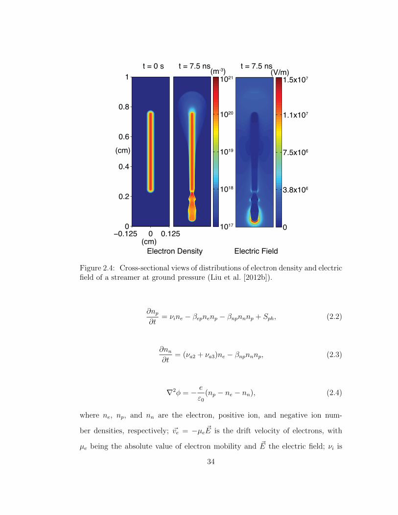
In a different study, Liu et al. [2012b] presented a modeling study on streamer
initiation from thundercloud hydrometeors in subbreakdown (below the con-
ventional breakdown threshold electric field) conditions. They conducted a
simulation for an electric field value of 0.5Ek at ground pressure. Their model
hydrometeor had a length of 5 mm and radius of 0.1 mm. They observed suc-
cessful streamer emission from this hydrometeor, as shown in Figure 2.4. The
figure shows cross-sections of electron density and electric field. Theirs was the
first theoretical study to show streamers are able to form from isolated model
hydrometeors in electric fields close to the measured thundercloud field.
2.3 Streamer Discharge Model
For the present study, we further investigate the idea proposed by Liu et al.
[2012b] to study streamers from hydrometeors in thundercloud conditions. To
describe the dynamics of a single streamer, we use the cylindrically symmetric
streamer discharge model developed by Liu and Pasko [2004]. In this model,
the streamer dynamics are described by the electron and ion drift-diffusion
equations coupled with Poisson’s equation:
∂ne∂t
+∇ · ne~ve −De∇2ne = (νi − νa2 − νa3)ne − βepnenp + Sph, (2.1)
33
t = 0 s
−0.125 0 0.125
1
0.8
0.6
0.4
0.2
0
(cm)
(cm)
t = 7.5 ns
1017
1018
1019
1020
1021
(m-3)t = 7.5 ns
0
3.8x10⁶
7.5x10⁶
1.1x10⁷
1.5x10⁷(V/m)
Electron Density Electric Field
Figure 2.4: Cross-sectional views of distributions of electron density and electricfield of a streamer at ground pressure (Liu et al. [2012b]).
∂np∂t
= νine − βepnenp − βnpnnnp + Sph, (2.2)
∂nn∂t
= (νa2 + νa3)ne − βnpnnnp, (2.3)
∇2φ = − e
ε0(np − ne − nn), (2.4)
where ne, np, and nn are the electron, positive ion, and negative ion num-
ber densities, respectively; ~ve = −µe ~E is the drift velocity of electrons, with
µe being the absolute value of electron mobility and ~E the electric field; νi is
34
the ionization frequency; νa2 and νa3 are the two-body and three-body elec-
tron attachment frequencies, respectively; βep and βnp are the electron-positive
ion and negative-positive ion recombination coefficients, respectively; De is the
electron diffusion coefficient; Sph is the electron-ion pair production rate due to
photoionization; φ is the electric potential; e is the absolute value of electron
charge; and ε0 is the permittivity of free space. Ions have much smaller mobili-
ties compared to electrons and for the timescales involved in this study (a few
tens of nanoseconds) they can be considered immobile. All the coefficients in
the model are functions of the reduced local electric field E/N , where E is the
magnitude of the electric field and N is the neutral air density. The coefficients
are obtained from the solution to the Boltzmann equation [Moss et al., 2006],
with a few exceptions discussed by Liu and Pasko [2004]. The photoionization
rate Sph is calculated using the methods developed in Bourdon et al. [2007] and
Liu et al. [2007]. The boundary conditions on the sides of the simulation region
are Dirichlet boundary conditions. The direct integral solution to the electric
potential is used to calculate the potential at the boundary [Liu and Pasko,
2006].
35
Chapter 3
Streamers from Ionization
Column Hydrometeors
3.1 Model Description
For this part of our study we model the hydrometeors using an isolated col-
umn consisting of free electrons and positive ions. The column consists of two
hemispherical caps attached onto a cylindrical body. The initial distributions of
electrons and positive ions in the column are described by the following equa-
tions:
for z > zt :
ne0(r, z) = np0(r, z) =n0
2[1 + tanh(
a−√r2 + (z − zt)2σ
)] (3.1)
for z < zb :
ne0(r, z) = np0(r, z) =n0
2[1 + tanh(
a−√r2 + (z − zb)2σ
)] (3.2)
36
and for zb < z < zt :
ne0(r, z) = np0(r, z) =n0
2[1 + tanh(
a− rσ
)] (3.3)
where zt and zb are the altitudes of the center of the top and bottom hemi-
spherical caps, respectively; n0 is the peak density; a represents the radius of
the column; and σ controls the sharpness of the distribution. Equations 3.1 and
3.2 represent the distribution in the two hemispherical caps, while equation 3.3
describes the cylindrical body. This column shape for the model hydrometeor
best models an elongated water drop or ice needle that is aligned with the direc-
tion of the thundercloud electric field. In Liu et al. [2012b], by approximating
the column as a perfect conductor, the required dimension of the column in
order for a streamer to be initiated was provided as a simple relation. We have
used their relation to estimate the required length for our hydrometeors. It is
noteworthy to mention that although Liu et al. [2012b] have used a Gaussian
profile for the initial distribution of electrons and positive ions in the column,
we have mostly used a hyperbolic tangent (tanh) profile for this study. This is
because the radius and sharpness of the column or the hemispherical cap are
separately controlled by σ and a, allowing flexibility in tuning the parameters
for reducing the simulation run time.
In addition, if we assume our hydrometeors to be liquid water filaments,
we can calculate an initial density for the model hydrometeor by allowing the
Maxwellian relaxation time of the column hydrometeor to be equal to the di-
electric relaxation time of liquid water. Liquid water has a dielectric relaxation
time (τD) on the order of tens of picoseconds [Raju, 2003]. Following the re-
37
lation τM = ε0/σ, where τM is the Maxwellian relaxation time of the column
and σ the conductivity, the column conductivity should be about 0.885 S/m, if
τM = τD and τD = 10−11 s. This conductivity yields an initial electron density
of 1×10²⁰ m−3 if the column is placed inside a uniform electric field E0 = 0.3Ek
at ground pressure, where E0 determines the mobility of electrons.
Using an ionization column in place of a liquid water or ice dielectric filament
is justified by the following reasons. First, both water and ice have a very high
dielectric constant. When they are polarized, the same field enhancement factor
can be obtained as a polarized dense plasma column. This is the most important
factor determining the streamer initiation. Second, the seed electrons initiat-
ing the electron avalanches that propagate toward the positive tip are entirely
created by photoionization of air molecules. The discharge activity around the
positive tip of a dielectric filament is therefore accurately modeled. In addition,
it can be expected that corona discharges surrounding both of the positive and
negative tips prior to streamer initiation create an ionization cover around each
tip, similar in nature to the ionization column. Finally, the timescale of ambient
field variation is much longer than the dielectric relaxation time of water and
ice. Steady-state polarization of the water and ice hydrometeors can therefore
be assumed, i.e., their dielectric constant takes its dc field value. However,
the space charge field varies on a much shorter timescale than the dielectric
relaxation time of ice, so inaccuracies might be introduced when modeling ice
particles by using an ionization column. Given that the space charge field is
highly localized and it quickly moves away from the ice particle, we assume the
inaccuracies are negligible but future studies are required to verify it.
38
3.2 Modeling Results for 0.5Ek
In this section, we present the results of our streamer simulations. We have
performed simulations for a 0.5Ek ambient electric field at thundercloud alti-
tudes and obtained successful streamer formation, thus confirming the work of
Liu et al. [2012b]. We place the model hydrometeor inside the simulation do-
main and apply a uniform ambient electric field E0 = 0.5Ek in the downward
direction to start the simulation, which simulates the electric field inside the
thundercloud. The simulation domain is placed at 7 km altitude in all of our
simulations, which fits within the range of lightning initiation altitudes (see
Section 1.1.6). However, the principal conclusions of this study stay the same
for other thundercloud altitudes. Note that Ek is about 1.4× 10⁶ V/m at 7 km
altitude.
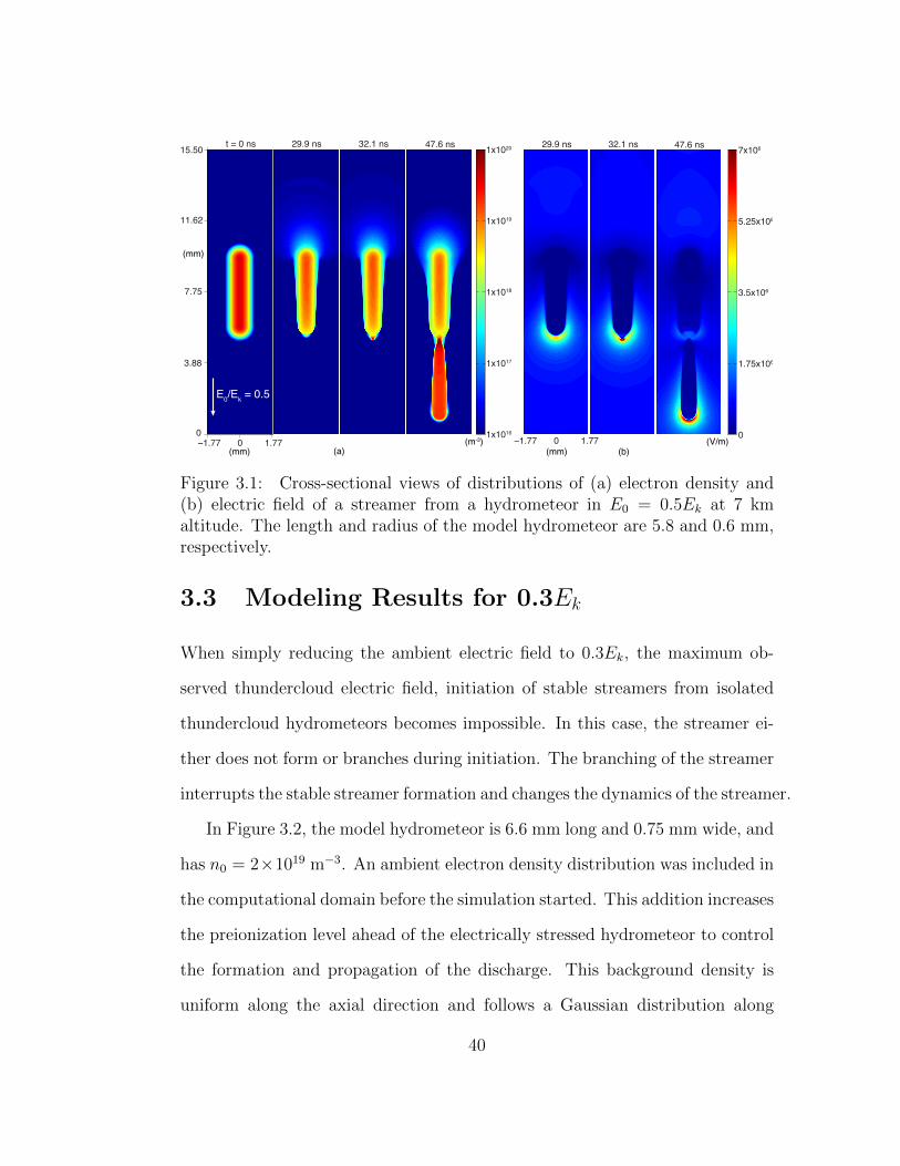
Figure 3.1 shows a model hydrometeor 5.8 mm long and 0.6 mm wide, with
an initial column density of n0 = 2 × 10¹⁹ m−3 (initial column density as cal-
culated in the previous section, scaled to 7 km altitude pressure, i.e., 1 × 10²⁰
m−3 (N/N0)2, where N and N0 are air densities at 7 km altitude and ground,
respectively). The figure shows cross-sections of electron density and electric
field distributions at a few different moments of time. At about 30 ns, the hy-
drometeor is nearly fully polarized and an enhanced electric field is present at
the positive tip. At 32.1 ns, the streamer is born from the positive tip. Each
panel shows a snapshot of the streamer, while propagating through the domain.
The last panel corresponding to 47.6 ns shows a fully formed streamer that has
stably propagated to the end of the simulation region.
39
t = 0 ns
−1.77 0 1.77
15.50
11.62
7.75
3.88
0
29.9 ns 32.1 ns 47.6 ns
1x10¹⁶
1x10¹⁷
1x10¹⁸
1x10¹⁹
1x10²⁰
E0/E
k = 0.5
(m-3)(mm)
(mm)
29.9 ns 32.1 ns
0
1.75x10⁶
3.5x10⁶
5.25x10⁶
7x10647.6 ns
(V/m)(mm) (b)(a)
−1.77 0 1.77
Figure 3.1: Cross-sectional views of distributions of (a) electron density and(b) electric field of a streamer from a hydrometeor in E0 = 0.5Ek at 7 kmaltitude. The length and radius of the model hydrometeor are 5.8 and 0.6 mm,respectively.
3.3 Modeling Results for 0.3Ek
When simply reducing the ambient electric field to 0.3Ek, the maximum ob-
served thundercloud electric field, initiation of stable streamers from isolated
thundercloud hydrometeors becomes impossible. In this case, the streamer ei-
ther does not form or branches during initiation. The branching of the streamer
interrupts the stable streamer formation and changes the dynamics of the streamer.
In Figure 3.2, the model hydrometeor is 6.6 mm long and 0.75 mm wide, and
has n0 = 2×10¹⁹ m−3. An ambient electron density distribution was included in
the computational domain before the simulation started. This addition increases
the preionization level ahead of the electrically stressed hydrometeor to control
the formation and propagation of the discharge. This background density is
uniform along the axial direction and follows a Gaussian distribution along
40
t = 0 ns
−1.77 0 1.77
15.50
11.62
7.74
3.88
0
(mm)
(mm)
27.7 ns
31.0 ns
47.6 ns
1x10¹⁶
1x10¹⁷
1x10¹⁸
1x10¹⁹
1x10²⁰
(m-3)
31.0 ns
47.6 ns
0
1.75x10⁶
3.5x10⁶
5.25x10⁶
7x10⁶
(V/m)(a) (b)
27.7 ns
−1.77 0 1.77(mm)
E0/E
k = 0.3
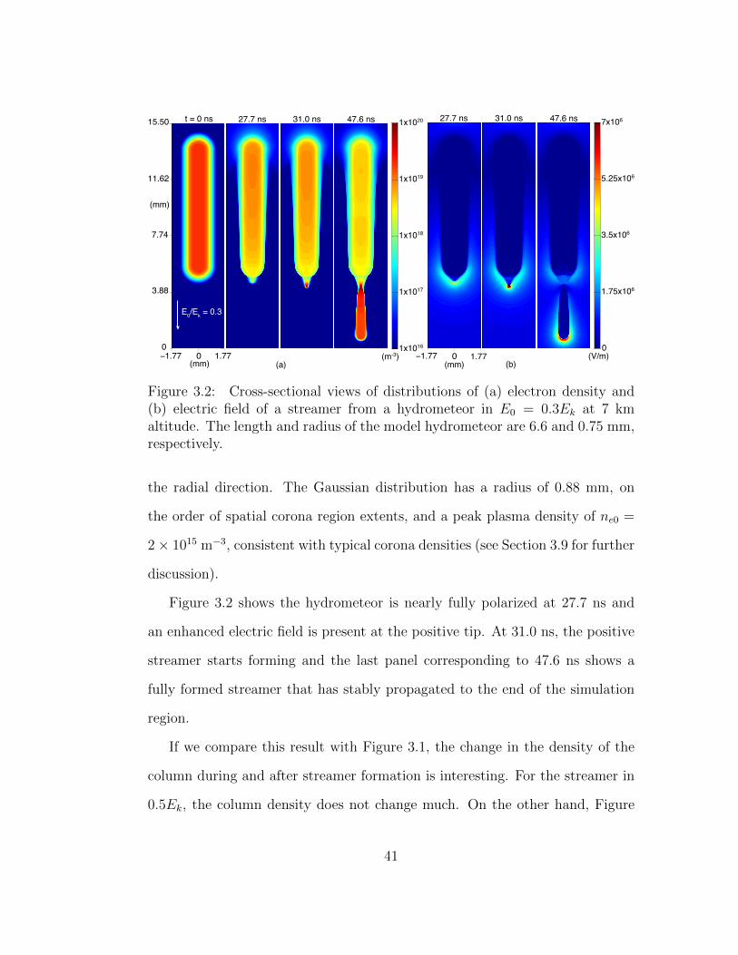
Figure 3.2: Cross-sectional views of distributions of (a) electron density and(b) electric field of a streamer from a hydrometeor in E0 = 0.3Ek at 7 kmaltitude. The length and radius of the model hydrometeor are 6.6 and 0.75 mm,respectively.
the radial direction. The Gaussian distribution has a radius of 0.88 mm, on
the order of spatial corona region extents, and a peak plasma density of ne0 =
2× 10¹⁵ m−3, consistent with typical corona densities (see Section 3.9 for further
discussion).
Figure 3.2 shows the hydrometeor is nearly fully polarized at 27.7 ns and
an enhanced electric field is present at the positive tip. At 31.0 ns, the positive
streamer starts forming and the last panel corresponding to 47.6 ns shows a
fully formed streamer that has stably propagated to the end of the simulation
region.
If we compare this result with Figure 3.1, the change in the density of the
column during and after streamer formation is interesting. For the streamer in
0.5Ek, the column density does not change much. On the other hand, Figure
41
3.2 shows an obvious drop in the column density. The processes that might
be responsible for changes in electron density of the column include two-body
electron attachment, three-body electron attachment, and recombination. A
simple estimation shows that three-body attachment is the dominant process
responsible for the density drop in the column, as shown in Figure 3.2. Assuming
the electric field in the column to be about 0.0025Ek, the three-body attachment
frequency at 7 km altitude is equal to 5.5 × 10⁷ s−1. Consequently, the three-
body attachment timescale is equal to about 18 ns, explaining the reduction in
density during the simulation time of 47 ns.
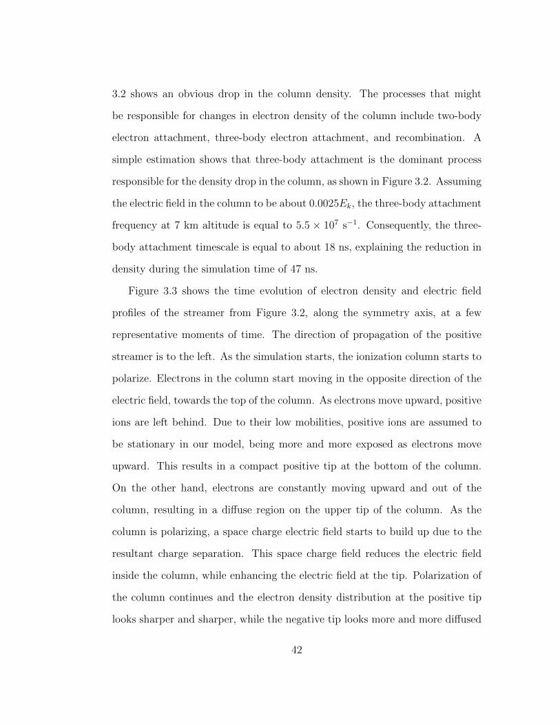
Figure 3.3 shows the time evolution of electron density and electric field
profiles of the streamer from Figure 3.2, along the symmetry axis, at a few
representative moments of time. The direction of propagation of the positive
streamer is to the left. As the simulation starts, the ionization column starts to
polarize. Electrons in the column start moving in the opposite direction of the
electric field, towards the top of the column. As electrons move upward, positive
ions are left behind. Due to their low mobilities, positive ions are assumed to
be stationary in our model, being more and more exposed as electrons move
upward. This results in a compact positive tip at the bottom of the column.
On the other hand, electrons are constantly moving upward and out of the
column, resulting in a diffuse region on the upper tip of the column. As the
column is polarizing, a space charge electric field starts to build up due to the
resultant charge separation. This space charge field reduces the electric field
inside the column, while enhancing the electric field at the tip. Polarization of
the column continues and the electron density distribution at the positive tip
looks sharper and sharper, while the negative tip looks more and more diffused
42
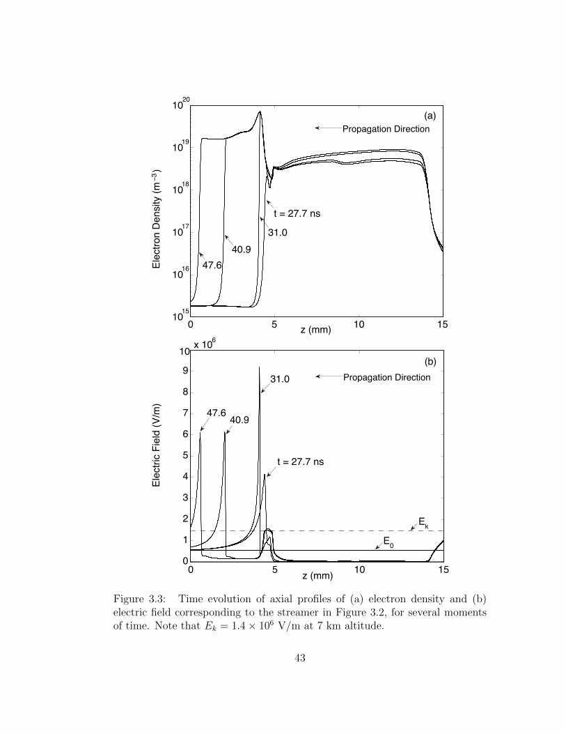
0 5 10 1510
15
1016
1017
1018
1019
1020
z (mm)
Ele
ctr
on
De
nsity (
m−
3)
t = 27.7 ns
31.0
40.9
47.6
(a)
0 5 10 150
1
2
3
4
5
6
7
8
9
x 106
z (mm)
Ele
ctr
ic F
ield
(V
/m)
31.0
t = 27.7 ns
40.947.6
10(b)
E0
Ek
Propagation Direction
Propagation Direction
Figure 3.3: Time evolution of axial profiles of (a) electron density and (b)electric field corresponding to the streamer in Figure 3.2, for several momentsof time. Note that Ek = 1.4× 10⁶ V/m at 7 km altitude.
43
due to electrons spreading outward. During this time, the electric field value
continues increasing at the positive tip. The bump in electron density around
z = 4.5 mm at 27.7 ns results from the ionization due to the highly enhanced
field at the positive tip. After 31 ns, the electric field at the hydrometeor
tip has increased to about 6.4Ek and starts to quickly move forward. At this
moment, the positive streamer is born from the positive tip. New electron
avalanches continuously move toward the streamer head, leaving a new positive
charge region behind and advancing the streamer head forward. The streamer
continues to propagate stably through the low field region until it reaches the
bottom of the domain. The streamer head field is about 4.25Ek during this
propagation stage, while the channel density is about 2× 10¹⁹ m−3.
3.4 Effects of Hydrometeor Dimension
According to the results obtained from our simulations, the dimension of the
model hydrometeor plays a significant role in the streamer initiation. As pre-
viously mentioned, in Liu et al. [2012b] the dimension required for streamer
initiation from an ionization column was estimated by treating the initial col-
umn as a perfect conductor. The required enhanced electric field Em at the
tip of a cylindrical conductor in a uniform electric field was assumed to be the
value of typical streamer head fields 3−5Ek, if the radius of the conductor takes
a value of typical streamer radii. This would result in the following relation:
l = a[ 10.56
(Em/E0 − 3)]1/0.92, where l and a are the length and radius of the
conductor, respectively.
Using this relation, with a radius equal to 0.75 mm, the length of the model
44
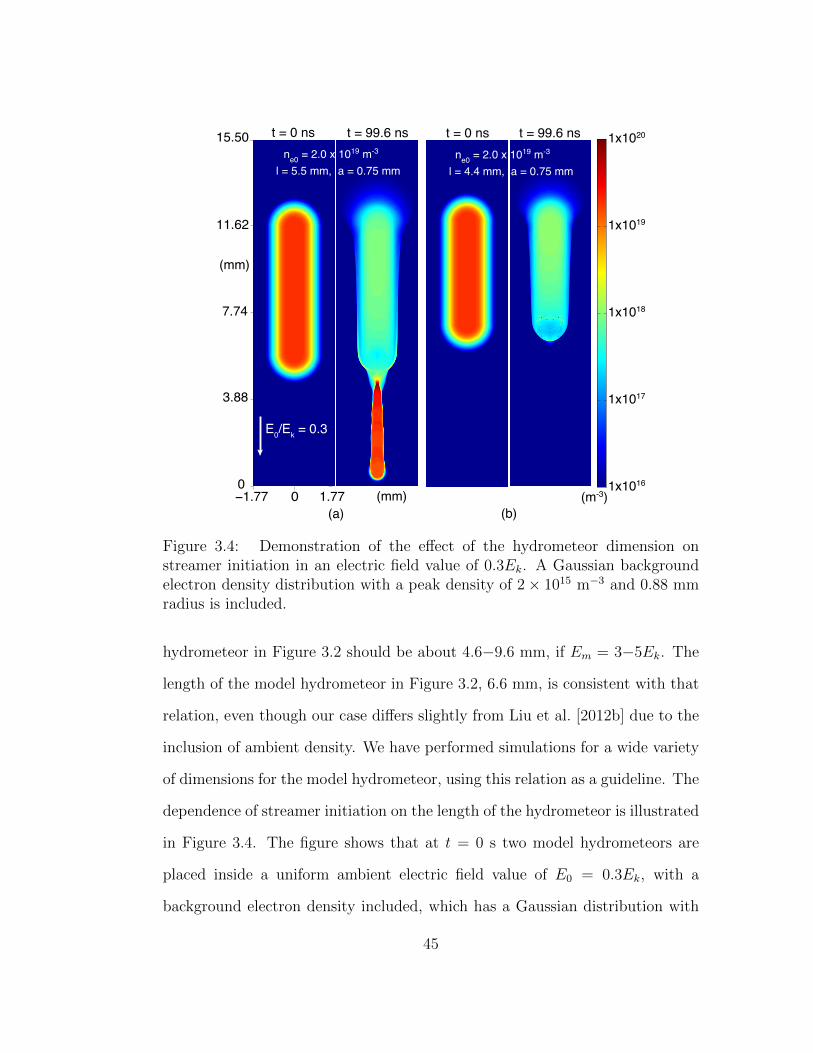
t = 0 ns
−1.77 0 1.77
15.50
11.62
7.74
3.88
0(mm)
(mm)
t = 99.6 ns
1x10¹⁶
1x10¹⁷
1x10¹⁸
1x10¹⁹
1x10²⁰
(m-3)
E0/E
k = 0.3
ne0
= 2.0 x 10¹⁹ m-3
l = 5.5 mm, a = 0.75 mm
t = 0 ns t = 99.6 ns
(a) (b)
l = 4.4 mm, a = 0.75 mm
ne0
= 2.0 x 10¹⁹ m-3
Figure 3.4: Demonstration of the effect of the hydrometeor dimension onstreamer initiation in an electric field value of 0.3Ek. A Gaussian backgroundelectron density distribution with a peak density of 2× 10¹⁵ m−3 and 0.88 mmradius is included.
hydrometeor in Figure 3.2 should be about 4.6−9.6 mm, if Em = 3−5Ek. The
length of the model hydrometeor in Figure 3.2, 6.6 mm, is consistent with that
relation, even though our case differs slightly from Liu et al. [2012b] due to the
inclusion of ambient density. We have performed simulations for a wide variety
of dimensions for the model hydrometeor, using this relation as a guideline. The
dependence of streamer initiation on the length of the hydrometeor is illustrated
in Figure 3.4. The figure shows that at t = 0 s two model hydrometeors are
placed inside a uniform ambient electric field value of E0 = 0.3Ek, with a
background electron density included, which has a Gaussian distribution with
45
a peak density of 2× 10¹⁵ m−3 and 0.88 mm radius. Both model hydrometeors
have the same radius and initial column density of 0.75 mm and 2× 10¹⁹ m−3,
respectively, as the simulation case for Figures 3.2 and 3.3. The hydrometeor
in the left panel of Figure 3.4 has a length of 5.5 mm, while the one in the right
panel has a length of 4.4 mm. After about 99.6 ns, from the two hydrometeors
that are identical otherwise, only the one with the longer length is able to initiate
a streamer. The length of the hydrometeor in the left panel is in agreement with
the estimate obtained by the relation.
However, additional simulation results show that streamers can be initiated
from the shorter hydrometeors when E0 is increased to 0.5Ek. The dependence
of the discharge initiation on the length of the sample hydrometeor has also
been shown by laboratory experiments. In the study by Griffiths and Latham
[1974], although they did not present a clear-cut relationship between Ec (critical
applied electric field necessary to initiate a streamer corona, as defined in that
study) and the length of the sample through their experiments, they concluded
that longer crystals have lower values of the critical applied field. In other words,
the critical applied field value required for streamer corona initiation is lower
when the length of the sample hydrometeor is longer. This is also suggested
by the relation between the required dimension and the applied field discussed
above.
3.5 Effects of Ambient Density
Introducing ambient electron density into our simulations promotes the forma-
tion of stable streamers in the ambient electric field of 0.3Ek. Recently, Qin and
46
Pasko [2014] show that the stable propagation of streamers originating from a
highly stressed electrode connected to an external circuit is not solely controlled
by the external field but also by the physical dimensions of streamers. Depend-
ing on different initial conditions (i.e., the dimension of the model hydrometeor,
and the magnitude and distribution of background density), the streamer initia-
tion from our model can result in a few different scenarios. One case is that the
streamer is able to form and propagate stably through the simulation domain
(Figure 3.2). For some cases, the forming streamer goes through pre-branching
and recovery stages many times. This results in an interesting form of the
streamer channel with fluctuating radius demonstrating the same variation of
the streamer head radius. We have named it a “wavy” streamer. The streamer
from Figure 3.4a is an example of such a case. Figure 3.5 shows the time evo-
lution of electric field profiles along the symmetry axis of this streamer. The
“wavy”-like structure of this streamer is more apparent from the profiles. For
this streamer, at some moments of time, for instance 76.3 ns, the transverse
radius of the streamer increases, and the streamer head flattens. At this point,
the streamer is in a pre-branching state, and the electric field in the streamer
head drops. After this widening, some streamers continue widening until the
streamer head splits. For this particular simulation case, after the widening of
the streamer head, the streamer recovers from the pre-branching stage, reduc-
ing its transverse radial size, and hence continuing propagation with one single
head. This process corresponds to the dips and rises in the streamer head elec-
tric field as shown in the time evolution of the axial electric field profiles, and
is repeated a few times throughout the streamer propagation.
The distribution of the background density is a key parameter for the stable
47
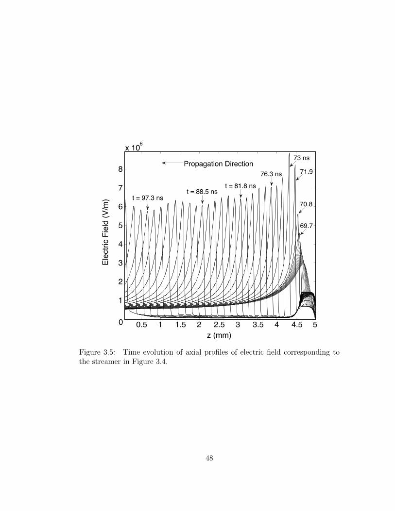
0.5 1 1.5 2 2.5 3 3.5 4 4.50
1
2
3
4
5
6
7
8
x 106
z (mm)
Ele
ctr
ic F
ield
(V
/m)
Propagation Direction73 ns
71.9
70.8
69.7
t = 97.3 nst = 88.5 ns
t = 81.8 ns
76.3 ns
5
Figure 3.5: Time evolution of axial profiles of electric field corresponding tothe streamer in Figure 3.4.
48
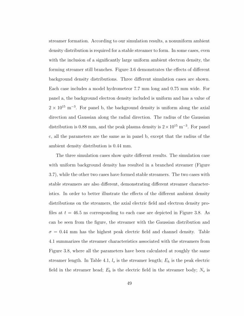
streamer formation. According to our simulation results, a nonuniform ambient
density distribution is required for a stable streamer to form. In some cases, even
with the inclusion of a significantly large uniform ambient electron density, the
forming streamer still branches. Figure 3.6 demonstrates the effects of different
background density distributions. Three different simulation cases are shown.
Each case includes a model hydrometeor 7.7 mm long and 0.75 mm wide. For
panel a, the background electron density included is uniform and has a value of
2 × 10¹⁵ m−3. For panel b, the background density is uniform along the axial
direction and Gaussian along the radial direction. The radius of the Gaussian
distribution is 0.88 mm, and the peak plasma density is 2×10¹⁵ m−3. For panel
c, all the parameters are the same as in panel b, except that the radius of the
ambient density distribution is 0.44 mm.
The three simulation cases show quite different results. The simulation case
with uniform background density has resulted in a branched streamer (Figure
3.7), while the other two cases have formed stable streamers. The two cases with
stable streamers are also different, demonstrating different streamer character-
istics. In order to better illustrate the effects of the different ambient density
distributions on the streamers, the axial electric field and electron density pro-
files at t = 46.5 ns corresponding to each case are depicted in Figure 3.8. As
can be seen from the figure, the streamer with the Gaussian distribution and
σ = 0.44 mm has the highest peak electric field and channel density. Table
4.1 summarizes the streamer characteristics associated with the streamers from
Figure 3.8, where all the parameters have been calculated at roughly the same
streamer length. In Table 4.1, ls is the streamer length; Eh is the peak electric
field in the streamer head; Eb is the electric field in the streamer body; Ns is
49
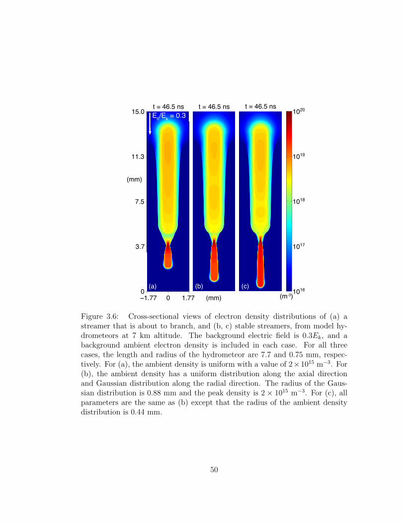
t = 46.5 ns
1016
1017
1018
1019
1020
(m-3)
(c)
−1.77 0 1.77
15.0
11.3
7.5
3.7
0
(mm)
(mm)
t = 46.5 ns t = 46.5 ns
(b)
E0/E
k = 0.3
(a)
Figure 3.6: Cross-sectional views of electron density distributions of (a) astreamer that is about to branch, and (b, c) stable streamers, from model hy-drometeors at 7 km altitude. The background electric field is 0.3Ek, and abackground ambient electron density is included in each case. For all threecases, the length and radius of the hydrometeor are 7.7 and 0.75 mm, respec-tively. For (a), the ambient density is uniform with a value of 2×10¹⁵ m−3. For(b), the ambient density has a uniform distribution along the axial directionand Gaussian distribution along the radial direction. The radius of the Gaus-sian distribution is 0.88 mm and the peak density is 2× 10¹⁵ m−3. For (c), allparameters are the same as (b) except that the radius of the ambient densitydistribution is 0.44 mm.
50
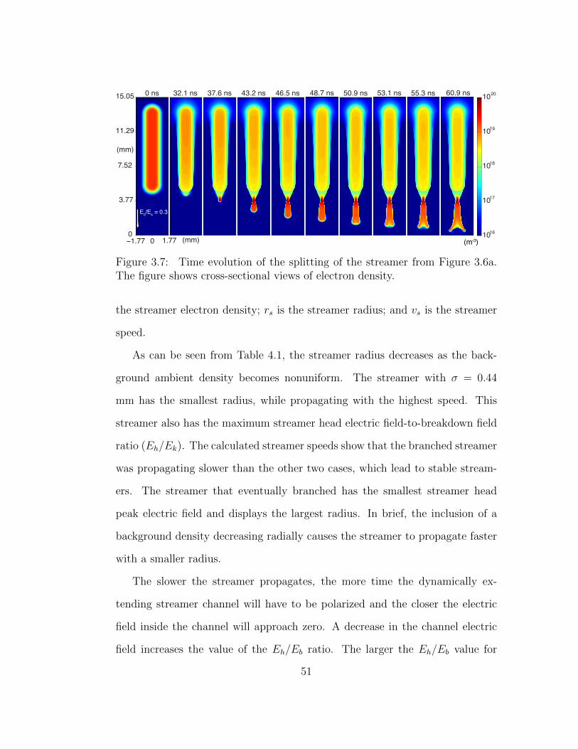
0 ns
−1.77 0 1.77
15.05
11.29
7.52
3.77
0(mm)
(mm)
32.1 ns
37.6 ns
43.2 ns
46.5 ns
50.9 ns
55.3 ns
60.9 ns
48.7 ns
53.1 ns
1016
1017
1018
1019
1020
(m-3)
E0/Ek = 0.3
Figure 3.7: Time evolution of the splitting of the streamer from Figure 3.6a.The figure shows cross-sectional views of electron density.
the streamer electron density; rs is the streamer radius; and vs is the streamer
speed.
As can be seen from Table 4.1, the streamer radius decreases as the back-
ground ambient density becomes nonuniform. The streamer with σ = 0.44
mm has the smallest radius, while propagating with the highest speed. This
streamer also has the maximum streamer head electric field-to-breakdown field
ratio (Eh/Ek). The calculated streamer speeds show that the branched streamer
was propagating slower than the other two cases, which lead to stable stream-
ers. The streamer that eventually branched has the smallest streamer head
peak electric field and displays the largest radius. In brief, the inclusion of a
background density decreasing radially causes the streamer to propagate faster
with a smaller radius.
The slower the streamer propagates, the more time the dynamically ex-
tending streamer channel will have to be polarized and the closer the electric
field inside the channel will approach zero. A decrease in the channel electric
field increases the value of the Eh/Eb ratio. The larger the Eh/Eb value for
51
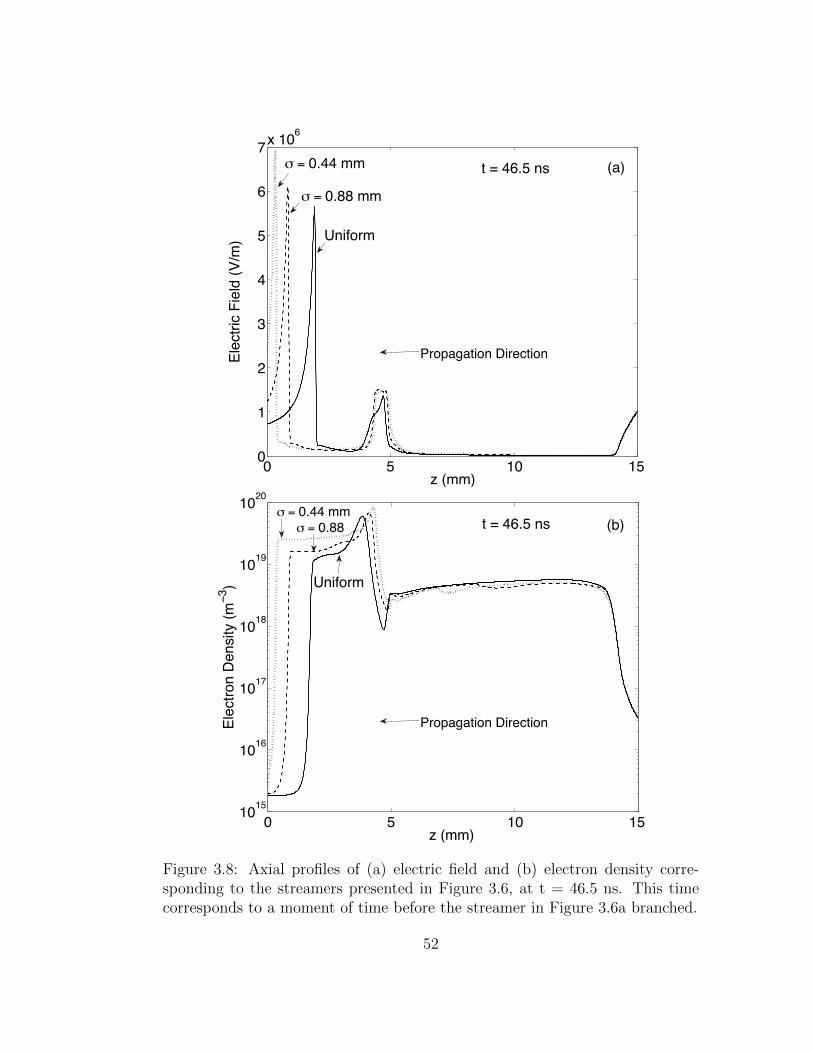
0 5 10 1510
15
1016
1017
1018
1019
1020
z (mm)
Ele
ctr
on
De
nsity (
m−
3)
Uniform
σ = 0.44 mm
0 5 10 150
1
2
3
4
5
6
7x 10
6
z (mm)
Ele
ctr
ic F
ield
(V
/m) Uniform
σ = 0.88 mm
σ = 0.44 mm (a)
(b)
Propagation Direction
t = 46.5 ns
Propagation Direction
t = 46.5 nsσ = 0.88
Figure 3.8: Axial profiles of (a) electric field and (b) electron density corre-sponding to the streamers presented in Figure 3.6, at t = 46.5 ns. This timecorresponds to a moment of time before the streamer in Figure 3.6a branched.
52
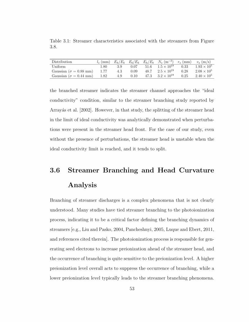
Table 3.1: Streamer characteristics associated with the streamers from Figure3.8.
Distribution ls (mm) Eh/Ek Eb/Ek Eh/Eb Ns (m−3) rs (mm) vs (m/s)Uniform 1.80 3.9 0.07 51.6 1.5× 10¹⁹ 0.33 1.93× 10⁵
Gaussian (σ = 0.88 mm) 1.77 4.3 0.09 48.7 2.5× 10¹⁹ 0.28 2.08× 10⁵
Gaussian (σ = 0.44 mm) 1.82 4.9 0.10 47.3 3.2× 10¹⁹ 0.25 2.40× 10⁵
the branched streamer indicates the streamer channel approaches the “ideal
conductivity” condition, similar to the streamer branching study reported by
Arrayas et al. [2002]. However, in that study, the splitting of the streamer head
in the limit of ideal conductivity was analytically demonstrated when perturba-
tions were present in the streamer head front. For the case of our study, even
without the presence of perturbations, the streamer head is unstable when the
ideal conductivity limit is reached, and it tends to split.
3.6 Streamer Branching and Head Curvature
Analysis
Branching of streamer discharges is a complex phenomena that is not clearly
understood. Many studies have tied streamer branching to the photoionization
process, indicating it to be a critical factor defining the branching dynamics of
streamers [e.g., Liu and Pasko, 2004, Pancheshnyi, 2005, Luque and Ebert, 2011,
and references cited therein]. The photoionization process is responsible for gen-
erating seed electrons to increase preionization ahead of the streamer head, and
the occurrence of branching is quite sensitive to the preionization level. A higher
preionization level overall acts to suppress the occurrence of branching, while a
lower preionization level typically leads to the streamer branching phenomena.
53
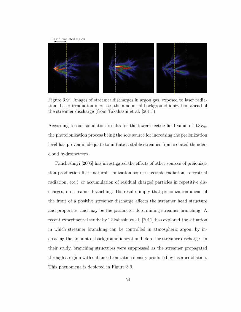
Laser irradiated region
Figure 3.9: Images of streamer discharges in argon gas, exposed to laser radia-tion. Laser irradiation increases the amount of background ionization ahead ofthe streamer discharge (from Takahashi et al. [2011]).
According to our simulation results for the lower electric field value of 0.3Ek,
the photoionization process being the sole source for increasing the preionization
level has proven inadequate to initiate a stable streamer from isolated thunder-
cloud hydrometeors.
Pancheshnyi [2005] has investigated the effects of other sources of preioniza-
tion production like “natural” ionization sources (cosmic radiation, terrestrial
radiation, etc.) or accumulation of residual charged particles in repetitive dis-
charges, on streamer branching. His results imply that preionization ahead of
the front of a positive streamer discharge affects the streamer head structure
and properties, and may be the parameter determining streamer branching. A
recent experimental study by Takahashi et al. [2011] has explored the situation
in which streamer branching can be controlled in atmospheric argon, by in-
creasing the amount of background ionization before the streamer discharge. In
their study, branching structures were suppressed as the streamer propagated
through a region with enhanced ionization density produced by laser irradiation.
This phenomena is depicted in Figure 3.9.
54
Inside thunderclouds, background ionization could be present due to several
mechanisms such as cosmic radiation, corona discharges, or electrons remaining
from a previous discharge. As a result, streamers may not be developing and
propagating through virgin air. In particular, other forms of electrical discharges
may have preceded the streamer initiation stage, causing enhancement in the
background ionization levels.
A more recent study by Savel’eva et al. [2013] has investigated the reasons for
branching of a positive streamer in a nonuniform electric field in a point-to-plane
electrode setup. They have found that flattening (or as they call it, “blunting”)
of the streamer head is a premonitory sign of branching, consistent with earlier
modeling studies [Arrayas et al., 2002, Liu and Pasko, 2004]. In a blunting
streamer, the maximum curvature of the streamer head is moving away from
the “pole” (the tip of the streamer head on the symmetry axis). As a result, the
maximum electric field and the maximum ionization rate shift away from the
symmetry axis as well. This causes the streamer to start branching at an angle
to the symmetry axis. In that study, a standard two-dimensional drift-diffusion
model is used to describe the streamer dynamics. They analyze the results of
their model in the context of a simplified analytical model for the streamer head.
In this analytical model, the streamer is approximated as an ideally conductive
semielliptical head with a cylindrical channel. It is assumed that the streamer
head grows due to ionization on its surface. The growth rate of a point on
the streamer head surface is determined mainly by the ionization frequency
of that surface point. The ionization frequency of each point depends on the
magnitude of the local electric field. For an ideal conductor, the distribution of
the electric field depends on its shape. So with a known shape for the streamer
55
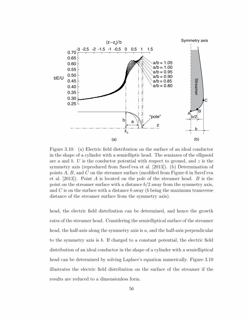
-30.70
0.65
0.60
0.55
0.50
0.45
0.40
0.35
0.30
0.25
-2.5 -2 -1.5 -1 -0.5 0 0.5 1 1.5
bE/U
(z –z0)/ b
a/b = 1.05a/b = 1.00a/b = 0.95a/b = 0.90a/b = 0.85a/b = 0.80
b
z0
az
“pole”
C
BA
b
Symmetry axis
Stre
am
er
b/2
(a) (b)
Figure 3.10: (a) Electric field distribution on the surface of an ideal conductorin the shape of a cylinder with a semielliptic head. The semiaxes of the ellipsoidare a and b. U is the conductor potential with respect to ground, and z is thesymmetry axis (reproduced from Savel’eva et al. [2013]). (b) Determination ofpoints A, B, and C on the streamer surface (modified from Figure 6 in Savel’evaet al. [2013]). Point A is located on the pole of the streamer head. B is thepoint on the streamer surface with a distance b/2 away from the symmetry axis,and C is on the surface with a distance b away (b being the maximum transversedistance of the streamer surface from the symmetry axis).
head, the electric field distribution can be determined, and hence the growth
rates of the streamer head. Considering the semielliptical surface of the streamer
head, the half-axis along the symmetry axis is a, and the half-axis perpendicular
to the symmetry axis is b. If charged to a constant potential, the electric field
distribution of an ideal conductor in the shape of a cylinder with a semielliptical
head can be determined by solving Laplace’s equation numerically. Figure 3.10
illustrates the electric field distribution on the surface of the streamer if the
results are reduced to a dimensionless form.
56
For a semi-spherical head (a = b), the maximum electric field is on the
symmetry axis, at the streamer head pole. From Figure 3.10a, for values of a
and b with a/b ≥ 0.95, the maximum electric field continues to remain at the
pole. However, for a/b ≤ 0.90, the maximum of the electric field shifts off of
the symmetry axis. In other words, for a sharp streamer head, the maximum
electric field remains on the pole, while for a blunt streamer head, the maximum
electric field shifts off-axis. This result also implies that the maximum electric
field does not necessarily move off-axis as soon as the streamer head deviates
from a semi-spherical form. It is only when b exceeds a by about 10% that the
maximum field starts to shift. With an initial semi-spherical streamer head, the
maximum electric field moves away from the pole in a rapidly widening streamer
provided that b grows faster than a, i.e., db/dt > da/dt. This conclusion has
been verified by their simulation results from the two-dimensional drift-diffusion
model.
According to the simulation results from the present study, flattening of the
streamer head is indeed a premonitory sign of streamer branching. In order
to analyze the surface dynamics of a streamer, we need to define the streamer
surface. One way to define the streamer surface is the points along the streamer’s
transverse direction with the maximum electric field value. Another can be the
points along the streamer’s transverse direction with the maximum value of
charge density. For the analysis presented here, we define the streamer surface
as the points along the streamer’s transverse direction, beyond the maximum
charge density, that are 1/e of this peak value. This definition results in a
smoother streamer surface in comparison with the others.
Using a similar convention as that used by Savel’eva et al. [2013], we focus
57
on three points A, B, and C on the streamer surface as shown in Figure 3.10b.
Point A is located on the pole of the streamer head. B is the point on the
streamer surface with a distance b/2 away from the symmetry axis, and C is on
the surface with a distance b away (b being the maximum transverse distance
of the streamer surface from the symmetry axis).
Considering the three streamer simulation cases presented in Figure 3.6,
Figure 3.11 shows the streamer surfaces for each of these cases, at different
moments of time. The three points A, B, and C are marked on each profile.
Figure 3.12 shows electric field values on the streamer surfaces corresponding to
each of the cases. For cases (b) and (c), all the profiles show the electric field on
the streamer surface is maximized at point A. Also, the maximum electric field
value stays about constant throughout the streamer propagation. On the other
hand, for case (a), initially at t = 44.3 ns, the surface electric field values drop
in the direction away from the streamer’s symmetry axis, with the maximum
field value being at point A. As time passes, the electric field value of point
A decreases, and the difference between A and B is reduced. At t = 48.7 ns,
the electric field at point B exceeds the value of point A and the maximum
field has shifted off of the symmetry axis. This trend continues as the streamer
propagates, moving the maximum electric field further and further away from
the axis. If we mark the time when the maximum electric field has moved off-
axis to be the branching initiation time, this streamer has started branching at
t = 48.7 ns.
In the study by Savel’eva et al. [2013], the maximum electric field moves off
of the symmetry axis after the maximum curvature of the streamer surface has
moved off-axis. We have performed a similar curvature analysis for our streamer
58
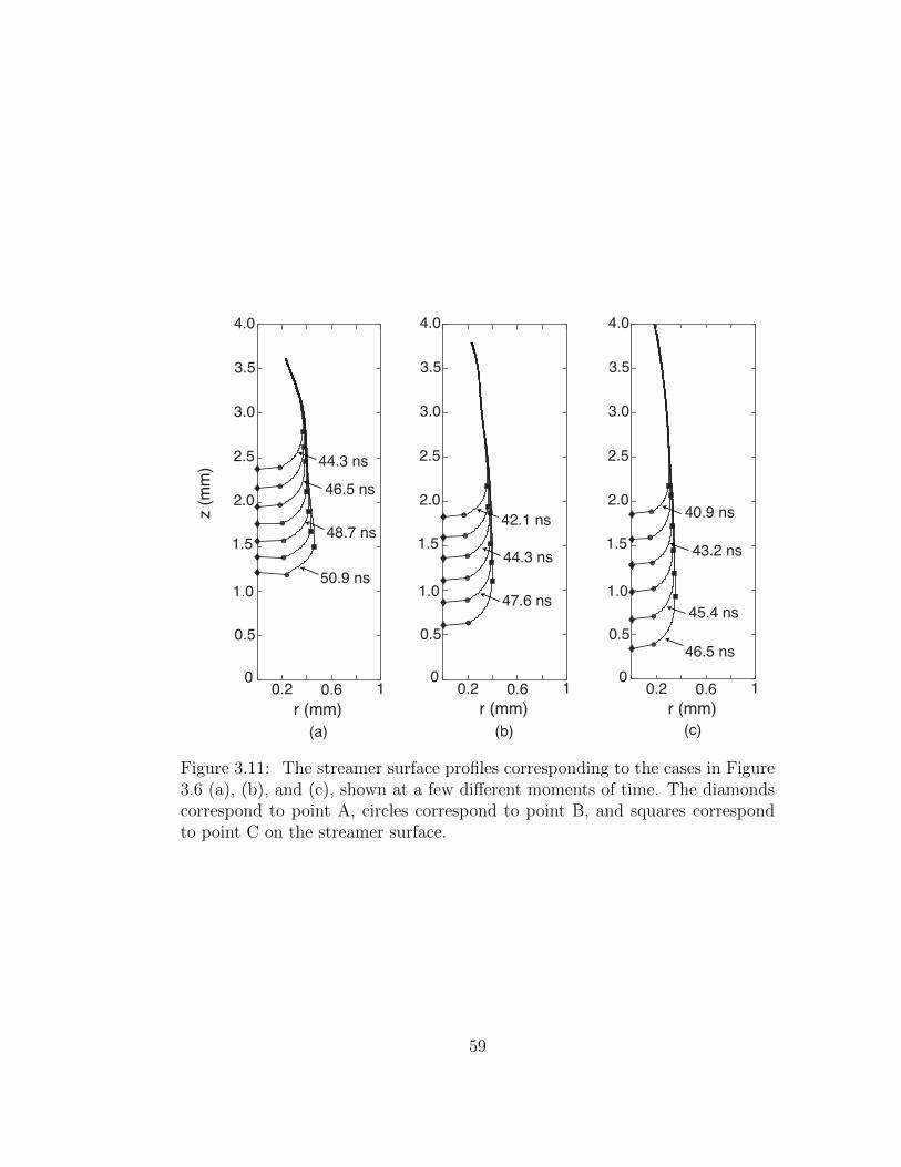
46.5 ns
40.9 ns
43.2 ns
45.4 ns
r (mm)
1.0
1.5
2.0
2.5
3.0
3.5
4.0
10
0.5
(c)
0.2 0.6
r (mm)
1.0
1.5
2.0
2.5
3.0
3.5
4.0
10
0.5
0.2 0.6
(b)
47.6 ns
44.3 ns
42.1 ns
r (mm)
1.0
1.5
2.0
2.5
3.0
3.5
4.0
10
0.5
0.2 0.6
(a)
48.7 ns
44.3 ns
46.5 ns
50.9 ns
z (
mm
)
Figure 3.11: The streamer surface profiles corresponding to the cases in Figure3.6 (a), (b), and (c), shown at a few different moments of time. The diamondscorrespond to point A, circles correspond to point B, and squares correspondto point C on the streamer surface.
59
simulation results. Figure 3.13 presents streamer surface curvature profiles cor-
responding to the same moments of time presented in Figures 3.11 and 3.12.
To calculate the curvature value for each point on the streamer surface, the
surface of the three-dimensional streamer body is obtained by rotating the two-
dimensional streamer surface profile around the symmetry axis. Each point on
the streamer surface may have different curvatures for different planes contain-
ing that point. Each curvature value measures how much the surface bends
along a particular tangential direction at that point. The principal curvatures
at each point on the surface, denoted by κ1 and κ2, are the maximum and min-
imum values of all the different curvature values at that point. In other words,
as defined in differential geometry, the principal curvatures are the eigenvalues
of the shape operator at that point. The average of the two principal curvatures
at every point is the mean curvature, denoted H, where H = 12(κ1 + κ2). We
use this definition for H to calculate the mean curvature (henceforth denoted
as “curvature”) of every point on the streamer surface, corresponding to the
moments of time presented in Figure 3.12.
Looking at Figure 3.13, the main feature that distinguishes our results from
Savel’eva et al. [2013] is that neither of the curvature profiles gives a maximum
value on the symmetry axis. This means that even at the beginning of the
streamer propagation, the streamer tip is not the sharpest point of the streamer
head. This is true even for the two streamer cases that do not branch at all.
For these two cases, our results show that the maximum electric field is on the
symmetry axis and until the end of the simulation, it does not shift off-axis
with the shifting of the maximum curvature. A common misconception is that
the electric field at the surface of an isolated conductor is greatest where the
60
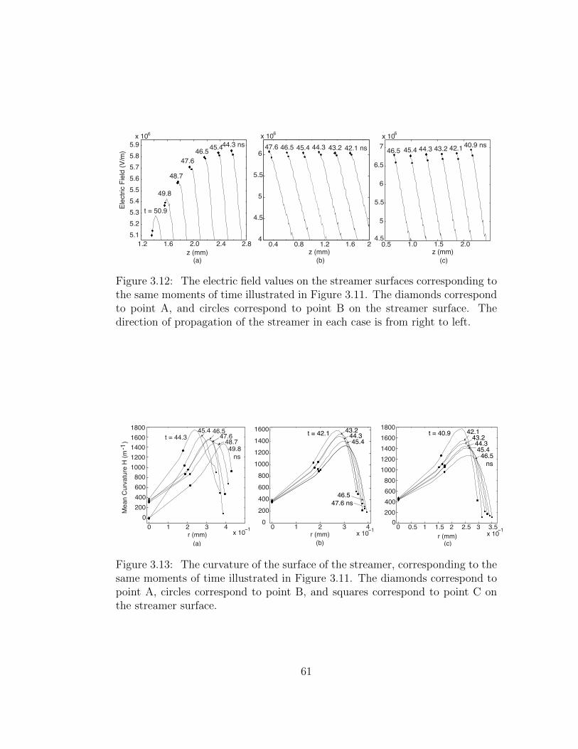
1.2 1.6 2.0 2.4 2.85.15.25.35.45.55.65.75.85.9
x 106
z (mm)
Elec
tric
Fiel
d (V
/m)
48.7
44.3 ns45.446.547.6
49.8
t = 50.9
0.4 0.8 1.2 1.6 24
4.5
5
5.5
6
x 106
z (mm)
47.6 44.345.446.5 43.2 42.1 ns
0.5 1.0 1.5 2.04.5
5
5.5
6
6.5
7x 10⁶
z (mm)
46.540.9 ns42.143.244.345.4
(a) (b) (c)
Figure 3.12: The electric field values on the streamer surfaces corresponding tothe same moments of time illustrated in Figure 3.11. The diamonds correspondto point A, and circles correspond to point B on the streamer surface. Thedirection of propagation of the streamer in each case is from right to left.
0200400600800
1000120014001600
0 0.5 1 1.5 2 2.5 3 3.5x 10⁻¹
0200400600800
10001200140016001800
r (mm)(a) (c)
48.745.4 46.5
47.6
49.8 ns
43.2t = 42.1 44.345.4
46.547.6 ns
t = 40.9 42.1 43.2 44.3 45.4
46.5 ns
0 1 2 3 4x 10⁻¹
0200400600800
10001200140016001800
r (mm)
Mea
n C
urva
ture
H (m
-1) t = 44.3
(b)
0 1 2 3 4x 10⁻¹r (mm)
Figure 3.13: The curvature of the surface of the streamer, corresponding to thesame moments of time illustrated in Figure 3.11. The diamonds correspond topoint A, circles correspond to point B, and squares correspond to point C onthe streamer surface.
61
curvature is greatest. In fact, it has been shown by Price and Crowley [1985]
that in general, these two maxima are located at different points on the surface.
This is based on the fact that these two parameters depend on the shape of
the surface in entirely different ways. Curvature depends only on the local
shape of the surface, while the electric field is determined by the charge density
distribution on the entire surface. Changing the shape of the surface away from
a particular point does not effect the curvature at that point. However, changing
the shape of the surface in one region influences the charge density distribution
over the entire surface. This suggests that the non-collocation of the maximum
curvature and maximum electric field cannot be the sole parameter responsible
for streamer branching, since the two streamer cases that have not exhibited
branching have not shown collocation of these two parameters either.
From Figure 3.13, a main feature of the branching streamer case (a) is that
the maximum curvature of the streamer surface moves away from the symmetry
axis with a faster rate than the other two cases. Focusing on the moments of
time before the streamer has branched (until t = 48.7 ns), the location of the
maximum curvature at the time of branching is considerably farther than the
first profile’s. The curvature profiles for the other two cases show much less
shifting of the maximum values, with some profiles hardly shifting at all. The
farther the maximum curvature value is from the symmetry axis, the flatter the
streamer head becomes. On the other hand, the two non-branching cases show a
fast drop in the maximum curvature value as time progresses. This is consistent
with acceleration and radial expansion of the streamer channel as it propagates
forward [Liu and Pasko, 2004]. The curvature profiles for the branching case,
however, do not show much reduction in the maximum values and the rate of
62
reduction is definitely less than the other two cases.
According to the discussion above, our simulation results suggest that the
geometry of the streamer head plays an important role in the streamer branch-
ing phenomena. The fast radial movement of the maximum streamer head
curvature, combined with the slow reduction of the maximum curvature values,
causes the streamer head to eventually pull the maximum electric field off of
the symmetry axis. The redistribution of the electric field profile with the max-
imum moving away from the axis is a critical turning point for the streamer
head. As the location of the maximum electric field is also the fastest growth
point of the streamer head surface, this phenomenon results in the streamer
propagating off-axis and hence branching.
3.7 Comparison with Realistic Hydrometeors
We have demonstrated that streamers can be initiated from model hydrometeors
in subbreakdown electric fields as low as 0.3Ek, which is a measured maximum
electric field value inside the thundercloud. It is also important that these hy-
drometeors possess similar physical properties as the hydrometeors present in
the thundercloud. A summary of different types of hydrometers and their cor-
responding dimensions can be found in Table 3.2. As discussed in Section 2.1,
the most favorable configurations for streamers to originate from hydromete-
ors have been concluded to be glancing collisions of two water drops [Crabb
and Latham, 1974] and individual ice crystals [Griffiths and Latham, 1974].
The simple columniform shape that we have chosen for our model hydrometeor
characterizes the geometries of both cases.
63
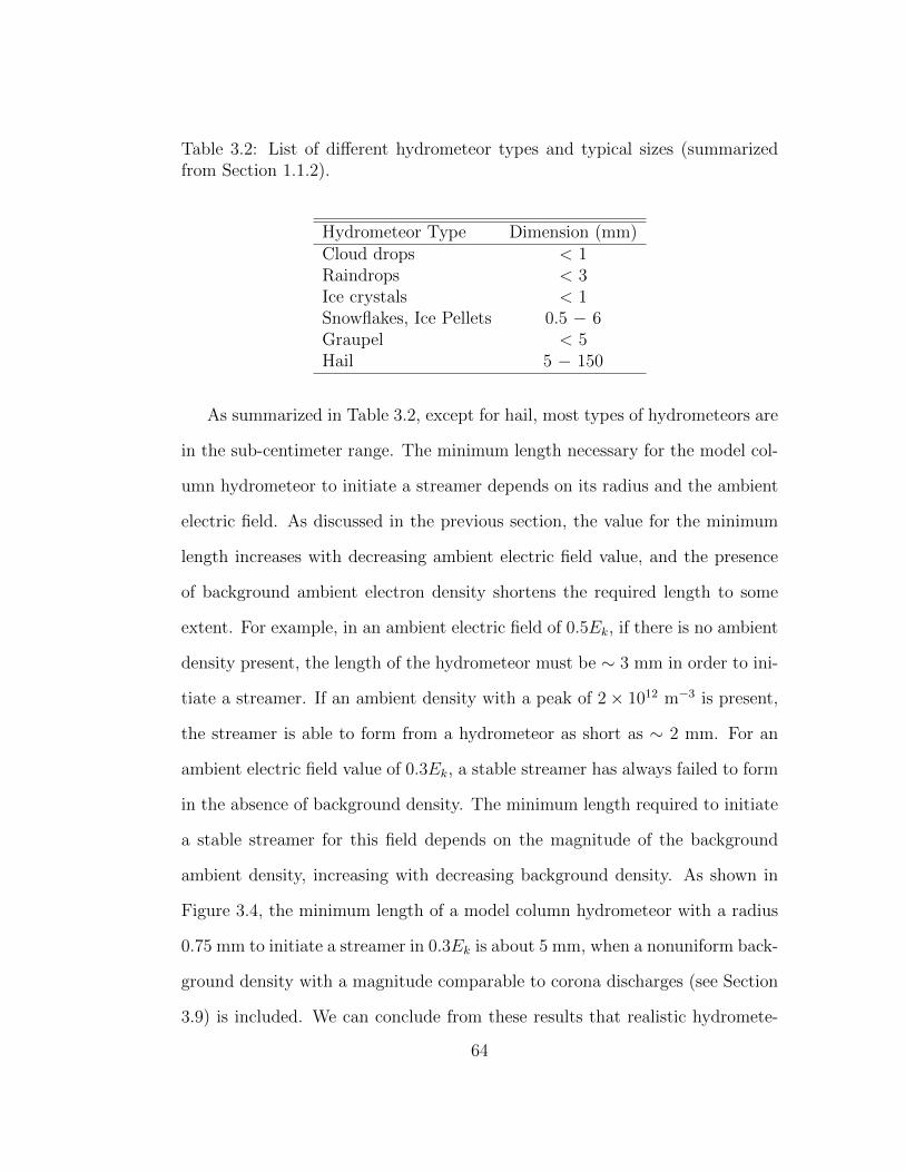
Table 3.2: List of different hydrometeor types and typical sizes (summarizedfrom Section 1.1.2).
Hydrometeor Type Dimension (mm)Cloud drops < 1Raindrops < 3Ice crystals < 1Snowflakes, Ice Pellets 0.5 − 6Graupel < 5Hail 5 − 150
As summarized in Table 3.2, except for hail, most types of hydrometeors are
in the sub-centimeter range. The minimum length necessary for the model col-
umn hydrometeor to initiate a streamer depends on its radius and the ambient
electric field. As discussed in the previous section, the value for the minimum
length increases with decreasing ambient electric field value, and the presence
of background ambient electron density shortens the required length to some
extent. For example, in an ambient electric field of 0.5Ek, if there is no ambient
density present, the length of the hydrometeor must be ∼ 3 mm in order to ini-
tiate a streamer. If an ambient density with a peak of 2× 10¹² m−3 is present,
the streamer is able to form from a hydrometeor as short as ∼ 2 mm. For an
ambient electric field value of 0.3Ek, a stable streamer has always failed to form
in the absence of background density. The minimum length required to initiate
a stable streamer for this field depends on the magnitude of the background
ambient density, increasing with decreasing background density. As shown in
Figure 3.4, the minimum length of a model column hydrometeor with a radius
0.75 mm to initiate a streamer in 0.3Ek is about 5 mm, when a nonuniform back-
ground density with a magnitude comparable to corona discharges (see Section
3.9) is included. We can conclude from these results that realistic hydromete-
64
ors can initiate streamers in the measured thundercloud electric fields, with the
presence of ambient ionization density.
3.8 Comparison with Laboratory Experiments
In this section, we compare the results of the present study with experiments
conducted on streamer emission from hydrometeors, discussed in Chapter 2.
In the work of Griffiths and Latham [1974], corona streamers initiated from
ice hydrometeors were studied. They experimentally determined the relation
between air pressure (P ) and the critical applied electric field (Ec) required to
produce corona streamers, for various ice specimen at −12◦C. They considered
ice needles, prismatic ice crystals, flat plates of ice, and hailstones as different
ice hydrometeor groups. The ice needles considered are the most similar case to
the model hydrometeors in the present study. For their experiments, they used
chambers that were carefully maintained at a constant temperature and the
desired pressure. The ice sample was placed inside the chamber with its long
axis parallel to the field lines. After the chamber was sealed, no other source
could contaminate the experiment. Then the electric field was turned on and
slowly increased until a corona streamer discharge was initiated from the sample.
The onset of the discharge was marked by the appearance of glow around the
ends of the sample. This was viewed from the window in the chamber lid, with
the room previously darkened to allow the eye to adapt. They reported the
range of lengths that can produce streamer activity around ice hydrometeors to
be between 4−17 mm, for a 0.3Ek ambient field at 7 km pressure.
From the results of our current study, the range of minimum hydrometeor
65
lengths necessary for streamer initiation has been obtained to be approximately
5−8 mm (for an ambient electric field value of 0.3Ek at 7 km with a background
density range between 1015 − 1017 m−3), which overlaps with the range reported
by Griffiths and Latham [1974]. This range fits into the upper boundary of
typical hydrometeor sizes listed in Table 3.2. In these experiments, the slowly
varying electric field inside the chamber results in corona discharges preceding
the streamer formation. This can be similar in nature to the ambient density
that we have included in our simulations.
Petersen et al. [2006] have also observed positive streamer discharges from
ice crystals grown under controlled temperature and pressure. The dimension
of the longer axis of the ice crystals in their study ranged from 0.5−2 mm for
thicker crystals, and from 2−3 mm for thinner crystals. In their experiments the
electric field values necessary to start positive streamer discharges were recorded
to be between 500 and 850 kV/m at ground pressure. This range is a bit smaller
than the value used in our study (960 kV/m at ground pressure). Similar to the
experiments conducted by Griffiths and Latham [1974], the potential difference
applied to the two parallel plate electrodes used to establish a uniform electric
field was increased manually. The threshold electric field was recorded upon
observation of luminous filamentary traces around the ice crystal, via the image
intensifier. The corona discharges occurring before streamers in these experi-
ments could be the cause of the difference between the threshold electric fields
reported in the literature (as low as 500 kV/m for a ∼ 2 mm long hydrometeor)
and our study. However, at present it is unclear how a stable streamer can be
formed at such a low magnitude electric field.
When streamers are fully formed, they are known to be able to propagate
66
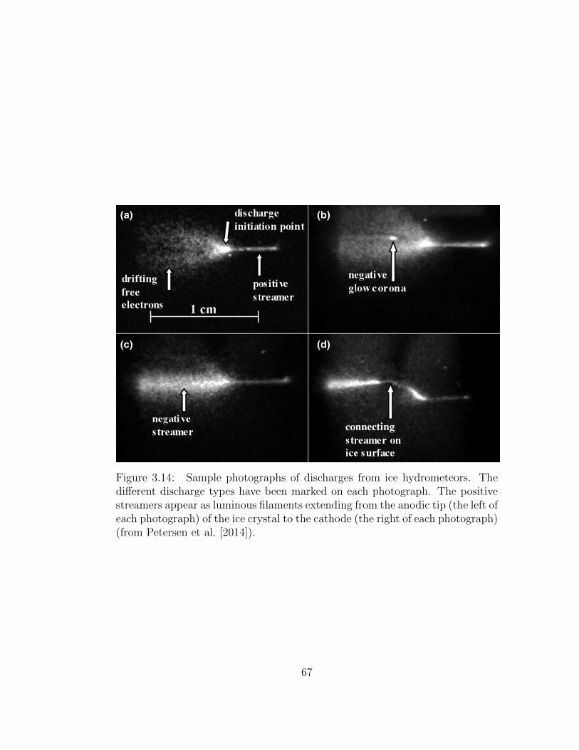
Figure 3.14: Sample photographs of discharges from ice hydrometeors. Thedifferent discharge types have been marked on each photograph. The positivestreamers appear as luminous filaments extending from the anodic tip (the left ofeach photograph) of the ice crystal to the cathode (the right of each photograph)(from Petersen et al. [2014]).
67
far even after branching, as shown by laboratory experiments on the discharges
originating from highly-stressed electrodes connected to a power supply [e.g.,
Nijdam et al., 2010]. However, experiments on streamers from isolated hydrome-
teors in an external electric field close to the measured thundercloud field display
a single channel that propagates without branching, much similar to what we
have observed from our simulation results. In particular, Petersen et al. [2014]
and Petersen et al. [2006], have observed positive streamer discharges from sim-
ulated ice hydrometeors in the laboratory. The positive streamers from their
study display a single illuminated channel moving from the ice hydrometeors
anodic tip into the electrode gap, as depicted in Figure 3.14.
Petersen et al. [2014] have observed different discharge types from glow
corona to positive and negative streamers, initiated from ice crystals. Figure 12
in that paper provides a plot of positive streamer threshold electric fields as a
function of ice crystal length for 570 mb pressure (about 5 km). The threshold
ambient field for positive streamer initiation from a 6−7 mm long ice crystal
is about 700 kV/m, which is in good agreement with our value of 0.3Ek = 550
kV/m.
Overall, the results presented here complement the experimental studies
mentioned above. The general trend of the decreasing electric field necessary
for streamer initiation with increasing hydrometeor length (Figure 3.4) obtained
from our study is consistent with the results of these studies, as well as with
other previous experimental and theoretical work [e.g., Crabb and Latham,
1974, Schroeder et al., 1999].
68
3.9 Role of Corona Discharges
An important conclusion from this study is that streamer initiation from realistic
thundercloud hydrometeors in a 0.3Ek electric field is impossible without the
presence of a nonuniform background electron density distribution. Corona
discharges inside the thundercloud can be a possible source for this ambient
density. Positive and negative corona discharges normally occur in the vicinity
of an electrically stressed discharge electrode. Chen and Davidson [2002] have
numerically determined the electron density distribution for a positive dc corona
discharge along a wire. The electron density distribution is obtained from the
1-D charge carrier continuity equations and Maxwell’s equation. In order to
study corona discharge in a wire-cylinder electrode geometry, the computational
domain is a thin cylindrical annulus, which only includes the plasma region.
For the wire-cylinder electrode setup, the corona discharge consists of a corona
plasma region directly around the high voltage electrode and a unipolar ion
region that is spread outward to the grounded electrode. The two regions are
separated by the ionization boundary, defined as the radial position where the
ionization coefficient and the attachment coefficient are equal. Electron number
density in the positive corona plasma was obtained for six different wire radii and
six linear current densities. For a 100 µm wire radius and a 100 µA/cm current
density, the electron density drops from 1015 m−3 at the wire surface to 1010 m−3
as the distance from the wire surface increases, up to 300 µm away. The electron
density increases with increasing current, and smaller electrodes produce thinner
plasmas, compared to those produced by larger wires. According to this study,
the provided range is sufficient to represent the most common uses of dc coronas.
Another study by Chen and Davidson [2003] has been conducted on negative
69
dc coronas. This study suggests that in negative corona, except very near the
surface of the wire, the density of electrons is nearly four orders of magnitude
greater than that in the positive corona. For a wire radius of 100 µm and a
current density of 100 µA/cm, the electron density increases from 1010 m−3 at
the wire surface to 1014 m−3 at 500 µm away. The electron density increases
with increasing gas temperature and current density.
Recently, Sin’kevich and Dovgalyuk [2014] have presented a review of the-
oretical and laboratory studies of corona discharge initiation in clouds. The-
oretical estimation of the rate of corona discharge appearance in clouds was
reviewed. This rate is necessary to estimate the role of corona discharges in the
formation of ambient density in the cloud. A study by Shishkin [1968] used a
simple numerical model of the cloud and assumed that each collision of large hy-
drometeors leads to a discharge. He showed that if the intensity of precipitation
in a cloud amounts to 10 mm/hr, the rate of collisions of large hydrometeors
and, correspondingly, the discharge rate per unit volume is equal to 10 m−3s−1.
Later studies [e.g., Stalevich and Uchevatkina, 1979a, 1979b, Shishkin, 1983]
considered that corona discharges will occur not only during collisions, but also
when hydrometeors approach each other. They estimated the approach number
for different distances between falling hydrometeors. This number is from 1018
up to 1030 times greater for small hydrometeors (radius = 0.2 mm) compared to
large ones (radius = 4−5 mm) when the precipitation intensity varies from 100
mm/h to 0.5 mm/h. This means that the approach rate per unit volume for
smaller hydrometeors is 1019 − 1031 m−3s−1. Since the lifetime of the electrons
at thundercloud altitudes is about 100 ns, the number of encounters will be
1012−1024 m−3. If we consider the volume of a corona discharge around a small
70
hydrometeor is about 10−9 m3, the number of encounters is 103−1015. Even if a
small fraction of these small hydrometeor encounters lead to corona discharges,
a persistent ionization may be expected in the thundercloud high field region.
It is noteworthy to mention that to the best of our knowledge, no recent papers
have been published on this subject.
The total number density of cloud particles is different for various types of
clouds as well as various types and sizes of hydrometeors. For water drops,
the total number of drops with diameters from 0.1−0.4 mm can be as large
as 108 m−3, which means that the average distance between two particles is
about 2 mm. From our simulation results, the cross-sectional area of the initial
streamer channel is about 0.3 mm2. Therefore, it is very likely that a streamer
will encounter a small hydrometeor after propagating through a short distance
on the order of a few mm. The total number density of large water drops with
diameters between 2−7 mm is about 104 m−3 with an average distance between
them about 4 cm. Hence, there will be a few small hydrometeors in the vicinity
of a large hydrometeor. This presents a great chance that corona discharges
will appear near a large hydrometeor, before streamer formation, and then in
the path of the streamer after it has formed.
According to the results of the studies discussed above, a nonuniform ambi-
ent density with a maximum value of 1015 m−3 may exist in a localized region
inside thunderclouds. The spatial extent of the corona region depends on the
discharge geometry and corona polarity, but the spatial scale in the transverse
direction of the background density distribution used in this study (∼ 400−800
µm) fits within the range of common coronas.
71
3.10 Role of Electron Detachment
The role of electron detachment from O− in increasing ionization in the upper
atmosphere has recently been studied [e.g., Luque and Gordillo-Vazquez, 2012,
Liu, 2012, and Neubert and Chanrion, 2013]. Liu [2012] investigated the role of
electron detachment from O− ions in sprite halo dynamics. This study indicates
that the detachment process affects the dynamics of the halo by allowing the
growth of electron density in the upper atmosphere under subbreakdown condi-
tions. Below, we show that this detachment process can be ignored for streamer
formation in subbreakdown fields at the thundercloud altitudes considered here.
O− ions are created by two-body dissociative electron attachment to molecu-
lar oxygen. However, for an ambient electric field of 0.3Ek at 7 km altitude, the
three-body electron attachment has a frequency of about 1.7×10⁶ s−1, while the
two-body electron attachment frequency is 2.2×10⁵ s−1, an order of magnitude
smaller than the three-body reaction. Consequently, the three-body attachment
reaction is faster, converting electrons to O2− ions. In addition, even when the
two-body attachment is faster than the three-body attachment, converting most
of the electrons to O− ions, at stronger electric fields, O− ions are mainly lost
due to a three-body attachment process transforming them to much more stable
ozone ions [Luque and Gordillo-Vazquez, 2012], instead of releasing electrons
through the detachment process. Therefore, the role of electron detachment
from O− ions can be ignored at thundercloud altitudes.
72
3.11 Negative Streamers
In this study, we have conducted simulations mainly for two electric field values
of 0.5Ek and 0.3Ek. The lengths of the ionization column hydrometeors used
vary between 4 and 10 mm, which is consistent with the dimension of ice crys-
tals and snowflakes presented in Table 3.2. For these simulations, the negative
streamer has always failed to form. This is also true for the case reported by
Liu et al. [2012b], and the sprite streamer initiation from ionization patches in
subbreakdown fields reported by Kosar et al. [2012] and Kosar et al. [2013]. For
sprite streamers, it has been discussed that positive streamers developing in an
electric field greater than their critical propagation field draw exponentially in-
creasing currents, which deposit a large amount of negative charge in the trail of
the streamer faster than the charge removed by the conducting trail [Liu, 2010].
Luque and Ebert [2010] have also suggested negative charging of the positive
sprite streamer channel, which may eventually lead to the emergence of negative
streamers. The positive streamers formed from our ionization column simula-
tions propagate very short distances, and the negative charging of the positive
streamer channel is not yet able to initiate negative streamers. This is due to
the high computational time that restricts the use of a longer computational
domain. It is very likely that continuous propagation of the positive streamer
from the ionization column may lead to initiation of negative streamers.
Experimental studies of Dawson [1969] (individual water drops) and Crabb
and Latham [1974] (colliding water drop filaments) also had difficulty producing
the negative streamer. However, it may as well be possible that the discharge
around the negative tip of a physical hydrometeor can not be resolved with our
current model. Replacing the ionization column by a dielectric hydrometeor
73

may offer a more accurate understanding of processes around the negative tip
to fully address the problem of the negative streamer initiation.
74
Chapter 4
Streamers from Dielectric
Hydrometeors
4.1 Dielectric Hydrometeor
For the first part of this dissertation study we used an ionization column in place
of a liquid water or ice dielectric filament. As discussed in Section 3.1, this is
justified in part by the high dielectric constant of water and ice. In this chapter,
we modify our streamer simulation model to accommodate an actual dielectric
water or ice particle. The inclusion of an actual dielectric material inside the
simulation domain results in a very complex dynamical model, because the
dielectric constant is not uniform anymore and a curved boundary is contained
in the simulation domain. We will describe the numerical models and methods
used to implement a dielectric hydrometeor into our model, and present the
results we have obtained.
75
4.2 Model Description
To simulate streamer initiation from a dielectric hydrometeor, we accommodate
a single isolated dielectric particle inside the simulation domain. This geometry
is different from previous streamer simulation studies where the electrodes lie
outside of the computational domain and/or are connected to an external circuit
[e.g., Liu and Pasko, 2004]. The model equations need to be solved throughout
the simulation domain in two different regions: outside the dielectric hydrom-
eteor, and inside. Outside of the dielectric hydrometeor, Poisson’s equation is
solved in order to find the electric field, and particle transport equations are
solved to obtain the distribution of space charges in the simulation domain (as
described in Section 2.3). Inside the dielectric hydrometeor, there is no free
charge density, so there is no need to solve particle transport equations, and
Poisson’s equation will reduce to Laplace’s equation.
The streamer model in our study has cylindrical symmetry, and a uniform
rectangular grid system is used for discretization of the model equations. When
including a dielectric particle inside the computational domain, the shape (e.g.,
sphere, ellipsoid, column, etc.) and physical state (e.g., liquid, solid) of the
hydrometeor play a defining role in choosing the numerical methods to solve the
model equations. Let’s assume that our shape of interest is a spherical dielectric.
Due to the inclusion of a spherical dielectric inside the computational domain,
uniform rectangular simulation cells will be cut by the curved boundary of the
hydrometeor. For these cells, part of the cell is inside the dielectric material,
while the other part is in air. Two key aspects that need to be considered
in this situation are: (1) accurate discretization of the governing equations
in the cells that are cut by the boundary, and (2) the imposition of proper
76
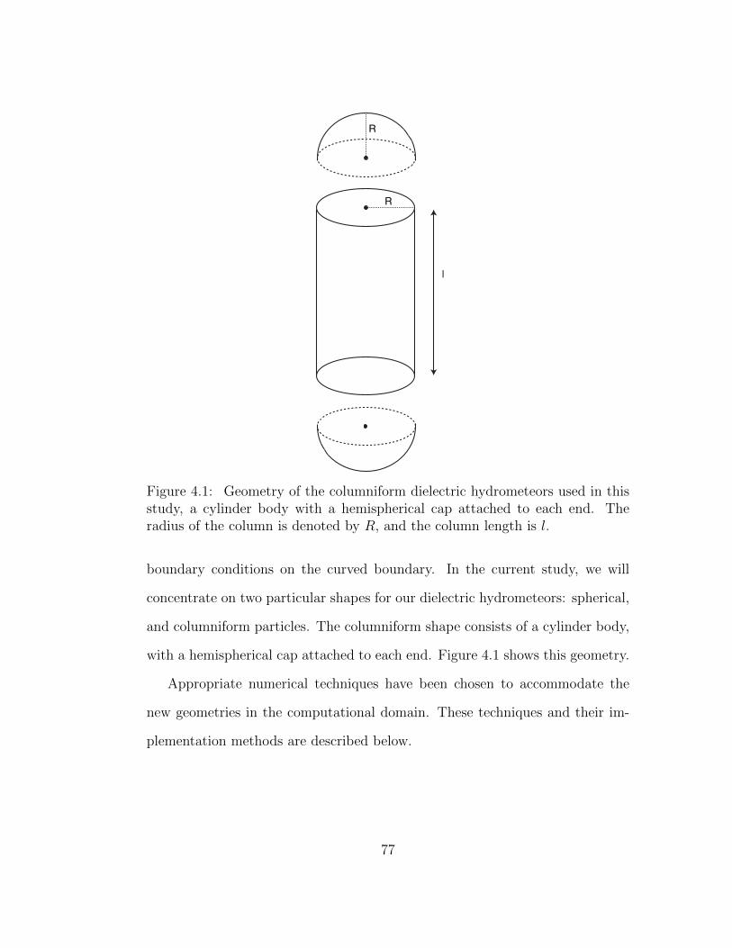
R
l
R
Figure 4.1: Geometry of the columniform dielectric hydrometeors used in thisstudy, a cylinder body with a hemispherical cap attached to each end. Theradius of the column is denoted by R, and the column length is l.
boundary conditions on the curved boundary. In the current study, we will
concentrate on two particular shapes for our dielectric hydrometeors: spherical,
and columniform particles. The columniform shape consists of a cylinder body,
with a hemispherical cap attached to each end. Figure 4.1 shows this geometry.
Appropriate numerical techniques have been chosen to accommodate the
new geometries in the computational domain. These techniques and their im-
plementation methods are described below.
77
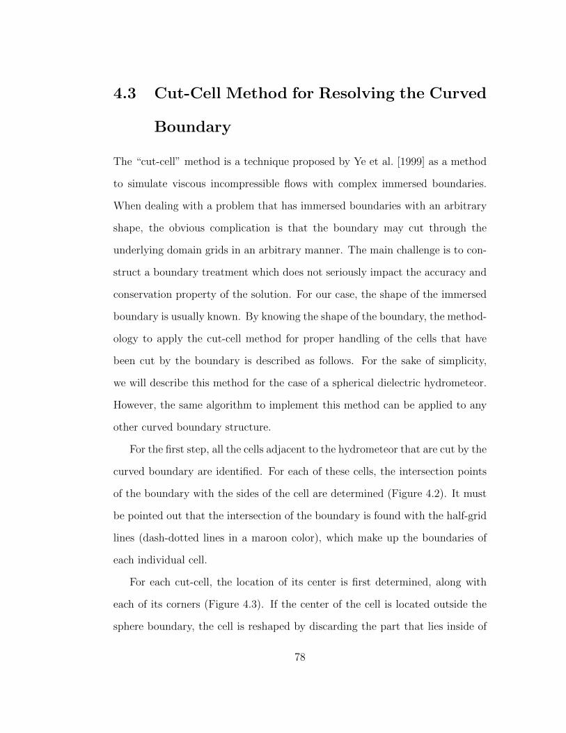
4.3 Cut-Cell Method for Resolving the Curved
Boundary
The “cut-cell” method is a technique proposed by Ye et al. [1999] as a method
to simulate viscous incompressible flows with complex immersed boundaries.
When dealing with a problem that has immersed boundaries with an arbitrary
shape, the obvious complication is that the boundary may cut through the
underlying domain grids in an arbitrary manner. The main challenge is to con-
struct a boundary treatment which does not seriously impact the accuracy and
conservation property of the solution. For our case, the shape of the immersed
boundary is usually known. By knowing the shape of the boundary, the method-
ology to apply the cut-cell method for proper handling of the cells that have
been cut by the boundary is described as follows. For the sake of simplicity,
we will describe this method for the case of a spherical dielectric hydrometeor.
However, the same algorithm to implement this method can be applied to any
other curved boundary structure.
For the first step, all the cells adjacent to the hydrometeor that are cut by the
curved boundary are identified. For each of these cells, the intersection points
of the boundary with the sides of the cell are determined (Figure 4.2). It must
be pointed out that the intersection of the boundary is found with the half-grid
lines (dash-dotted lines in a maroon color), which make up the boundaries of
each individual cell.
For each cut-cell, the location of its center is first determined, along with
each of its corners (Figure 4.3). If the center of the cell is located outside the
sphere boundary, the cell is reshaped by discarding the part that lies inside of
78
Figure 4.2: Cells that are cut by the boundary are identified and the intersectionof the boundary with the sides of these cut cells are determined (black dots).The solid black lines are the simulation domain grid lines, and the dash-dottedlines in maroon are the half-grid lines which make up the boundaries of theindividual cells.
79
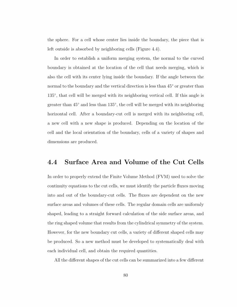
the sphere. For a cell whose center lies inside the boundary, the piece that is
left outside is absorbed by neighboring cells (Figure 4.4).
In order to establish a uniform merging system, the normal to the curved
boundary is obtained at the location of the cell that needs merging, which is
also the cell with its center lying inside the boundary. If the angle between the
normal to the boundary and the vertical direction is less than 45◦ or greater than
135◦, that cell will be merged with its neighboring vertical cell. If this angle is
greater than 45◦ and less than 135◦, the cell will be merged with its neighboring
horizontal cell. After a boundary-cut cell is merged with its neighboring cell,
a new cell with a new shape is produced. Depending on the location of the
cell and the local orientation of the boundary, cells of a variety of shapes and
dimensions are produced.
4.4 Surface Area and Volume of the Cut Cells
In order to properly extend the Finite Volume Method (FVM) used to solve the
continuity equations to the cut cells, we must identify the particle fluxes moving
into and out of the boundary-cut cells. The fluxes are dependent on the new
surface areas and volumes of these cells. The regular domain cells are uniformly
shaped, leading to a straight forward calculation of the side surface areas, and
the ring shaped volume that results from the cylindrical symmetry of the system.
However, for the new boundary cut cells, a variety of different shaped cells may
be produced. So a new method must be developed to systematically deal with
each individual cell, and obtain the required quantities.
All the different shapes of the cut cells can be summarized into a few different
80
Figure 4.3: The centers of the cells cut by the curved boundary (light bluedots) are identified along with their corners (dark blue dots).
81
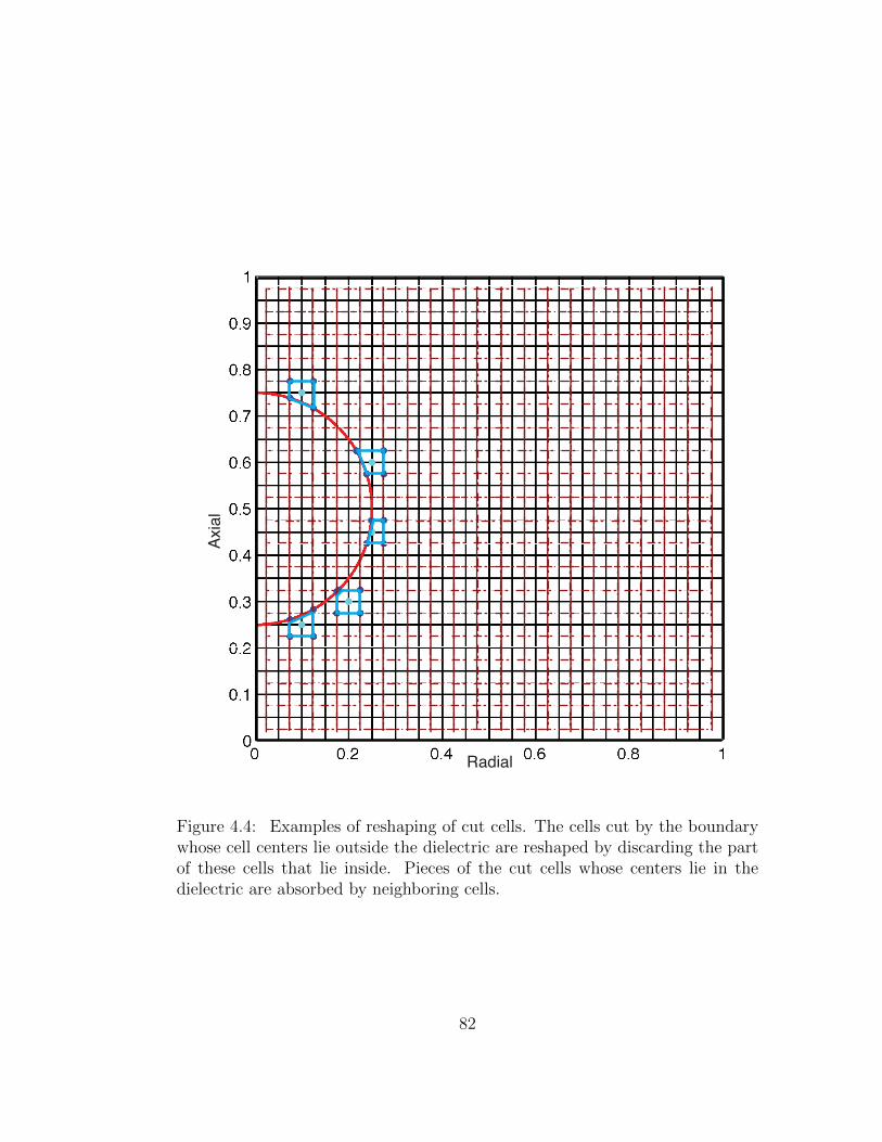
Radial
Axial
Figure 4.4: Examples of reshaping of cut cells. The cells cut by the boundarywhose cell centers lie outside the dielectric are reshaped by discarding the partof these cells that lie inside. Pieces of the cut cells whose centers lie in thedielectric are absorbed by neighboring cells.
82
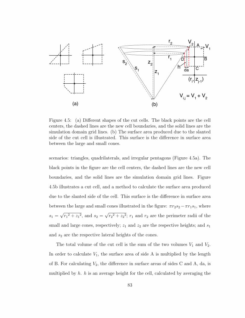
r2
z2
r1
z1
(a) (b)
(ri, z
j-1)
V2
V1
Vi,j
= V1 + V
2
s2
s1
h
A
B
C
D
da
Figure 4.5: (a) Different shapes of the cut cells. The black points are the cellcenters, the dashed lines are the new cell boundaries, and the solid lines are thesimulation domain grid lines. (b) The surface area produced due to the slantedside of the cut cell is illustrated. This surface is the difference in surface areabetween the large and small cones.
scenarios: triangles, quadrilaterals, and irregular pentagons (Figure 4.5a). The
black points in the figure are the cell centers, the dashed lines are the new cell
boundaries, and the solid lines are the simulation domain grid lines. Figure
4.5b illustrates a cut cell, and a method to calculate the surface area produced
due to the slanted side of the cell. This surface is the difference in surface area
between the large and small cones illustrated in the figure: πr2s2−πr1s1, where
s1 =√r12 + z12, and s2 =
√r22 + z22; r1 and r2 are the perimeter radii of the
small and large cones, respectively; z1 and z2 are the respective heights; and s1
and s2 are the respective lateral heights of the cones.
The total volume of the cut cell is the sum of the two volumes V1 and V2.
In order to calculate V1, the surface area of side A is multiplied by the length
of B. For calculating V2, the difference in surface areas of sides C and A, da, is
multiplied by h. h is an average height for the cell, calculated by averaging the
83
lengths of B and D. Based on the method of section 4.3, all the required cell
information has been recorded. This information includes the position of the
cell center and each of the cell corners, as well as the cell location with respect to
the spherical boundary. Equipped with this information, values of parameters
like r1, z1, and the length of each of the sides of the cell can easily be obtained.
Following a similar approach for each individual cut cell, the appropriate surface
areas and volumes of these cells can be collected.
4.5 Continuity Equation Solution Around the
Curved Boundary
The continuity equations of the streamer model have been solved using a fi-
nite volume method [Liu and Pasko, 2004]. These methods are commonly used
in solving problems of fluid dynamics and are especially designed to solve hy-
perbolic partial differential equation systems where discontinuities of physical
quantities or extremely high gradients of those quantities are present. They
are based on the integral form of the hyperbolic system. Instead of pointwise
approximations at grid points, the study domain is broken into grid cells and
the particle density in each cell is an average value, approximated by dividing
the total number of particles in the cell by the volume of the cell [LeVeque,
2002].
The streamer model equations have been discretized on a uniform, cylindri-
cally symmetric grid system. The solutions of the continuity equations are based
on keeping track of the total number of particles in each of the grid cells. At
each time step, these values are updated by using the value of the particle flux,
84
through the boundaries of each grid cell. A numerical scheme called the mod-
ified Scharfetter-Gummel method is used to calculate the particle flux density
[Liu and Pasko, 2004]. This method is a discretization scheme for variables in
convection-dominated or particle drifting-dominated problems, which employs
an exponential fitting technique to characterize the rapid density variation in
neighboring cells [Scharfetter and Gummel, 1969, and Kulikovsky, 1995].
4.5.1 Particle Flux Calculation and Boundary Conditions
After properly resolving the local geometrical parameters for the boundary-cut
cells, the next key issue is to accurately evaluate the particle fluxes moving into
and out of these cells. Figure 4.6 shows examples of reshaped boundary-cut
cells, along with arrows indicating the fluxes on each side of the cell. The dark
shaded arrows correspond to the fluxes that need special treatment.
Considering the reshaped boundary-cut cell in Figure 4.6, we describe the
method used to calculate the flux component due to electron drift, ~J = −µe ~Ene,
below. The figure shows four primary components for flux on the sides of the
boundary cell, ~FP , ~FS, ~GP , and ~GM , each component pointing to the direction
of positive flux. From here forth we will drop the vector sign, referring only
to the absolute values of the particle flux. GP can be broken down into two
separate components, GP1 and GP2. For each side, the related flux component
is calculated at the center of the side. The “donor-cell” or “upwind” method
is used to calculate these irregular flux components, by estimating the electric
field, mobility, and electron density from one side of the cell surface. Focusing
on GP1, the electric field and electron mobility values at the center of AB can
be calculated by linear extrapolation, provided that the values for correspond-
85
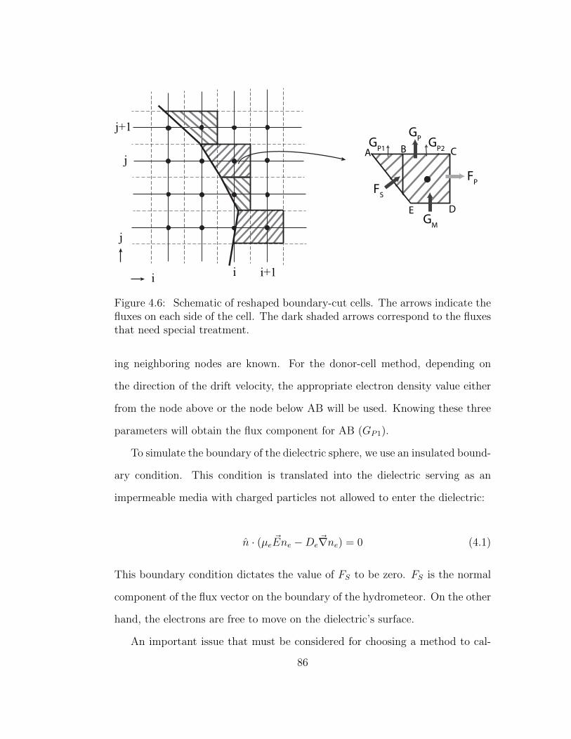
j
ii
j
j+1
i+1
GPG
P2
FS
FP
GM
GP1
A CB
DE
Figure 4.6: Schematic of reshaped boundary-cut cells. The arrows indicate thefluxes on each side of the cell. The dark shaded arrows correspond to the fluxesthat need special treatment.
ing neighboring nodes are known. For the donor-cell method, depending on
the direction of the drift velocity, the appropriate electron density value either
from the node above or the node below AB will be used. Knowing these three
parameters will obtain the flux component for AB (GP1).
To simulate the boundary of the dielectric sphere, we use an insulated bound-
ary condition. This condition is translated into the dielectric serving as an
impermeable media with charged particles not allowed to enter the dielectric:
n · (µe ~Ene −De~∇ne) = 0 (4.1)
This boundary condition dictates the value of FS to be zero. FS is the normal
component of the flux vector on the boundary of the hydrometeor. On the other
hand, the electrons are free to move on the dielectric’s surface.
An important issue that must be considered for choosing a method to cal-
86
culate the irregular flux components around the cut cells is assuring particle
flux balance between adjacent cells. This can be a bit tricky, due to the use
of different methods of flux calculation for different sides of a single cut cell,
and different methods may have different order of accuracies. For example, in
Figure 4.6, FP is calculated using the modified Scharfetter- Gummel method,
while GP and GM are calculated using a combination of the donor-cell method
with linear extrapolation, and FS is set to zero due to the boundary condition.
The results from the combination of methods that we have chosen here have
been carefully monitored and tested, and have proven accurate.
4.6 Electric Field Calculation Around the
Curved Boundary
In the streamer model, the electric field of the system is calculated by numer-
ically solving Poisson’s equation, transformed into a set of linear differential
equations upon discretization. The successive over-relaxation method (SOR) is
used to find the solution of this linear differential equation system, which gives
the electric potential. The electric field calculation is dependent on the physical
state of the dielectric particle. We have modified the electric field calculation to
accommodate two states of a hydrometeor: solid ice crystals and liquid water
filaments. The method and implementation details for each state is discussed
below.
87
4.6.1 Contant Polarization: Solid Ice Particles
To simulate solid ice hydrometeors, we have assumed the dielectric achieves
steady-state polarization at the beginning of the simulation, and the polarization
state is unvarying over time. This assumption is justified by the relatively
large dielectric relaxation time of ice (∼ 10−4 s) [Raju, 2003] compared to the
simulation time (∼ 10−9 s). Assuming the solid ice hydrometeor is in the shape
of a sphere, the electric field produced by a uniformly polarized dielectric sphere
with dielectric constant ε in a uniform electric field E0 is as follows:
~Ein =3
ε/ε0 + 2E0z r < R, (4.2)
~Eout = [1− (ε/ε0 − 1
ε/ε0 + 2)R3
r3 + 3(ε/ε0 − 1
ε/ε0 + 2)R3
r5 z2]E0z
+ [3(ε/ε0 − 1
ε/ε0 + 2)R3
r5 zr]E0r r > R (4.3)
where R is the radius of the sphere; r and z are the horizontal and vertical
coordinates, respectively; r is the distance from the point of interest to the
center of the sphere and can be written as√r2 + z2; and ~Ein and ~Eout are the
electric fields inside and outside of the dielectric sphere, respectively.
Figure 4.7 shows a schematic illustration of the simulation domain, includ-
ing the spherical dielectric hydrometeor, located inside a uniform electric field
distribution. At every point inside the simulation region, the electric field has
three components; the uniform ambient Laplacian field, the electric field due to
the polarized dielectric sphere, and the electric field generated by space charges.
The first two components are calculated using Equations 4.2 and 4.3. These val-
88
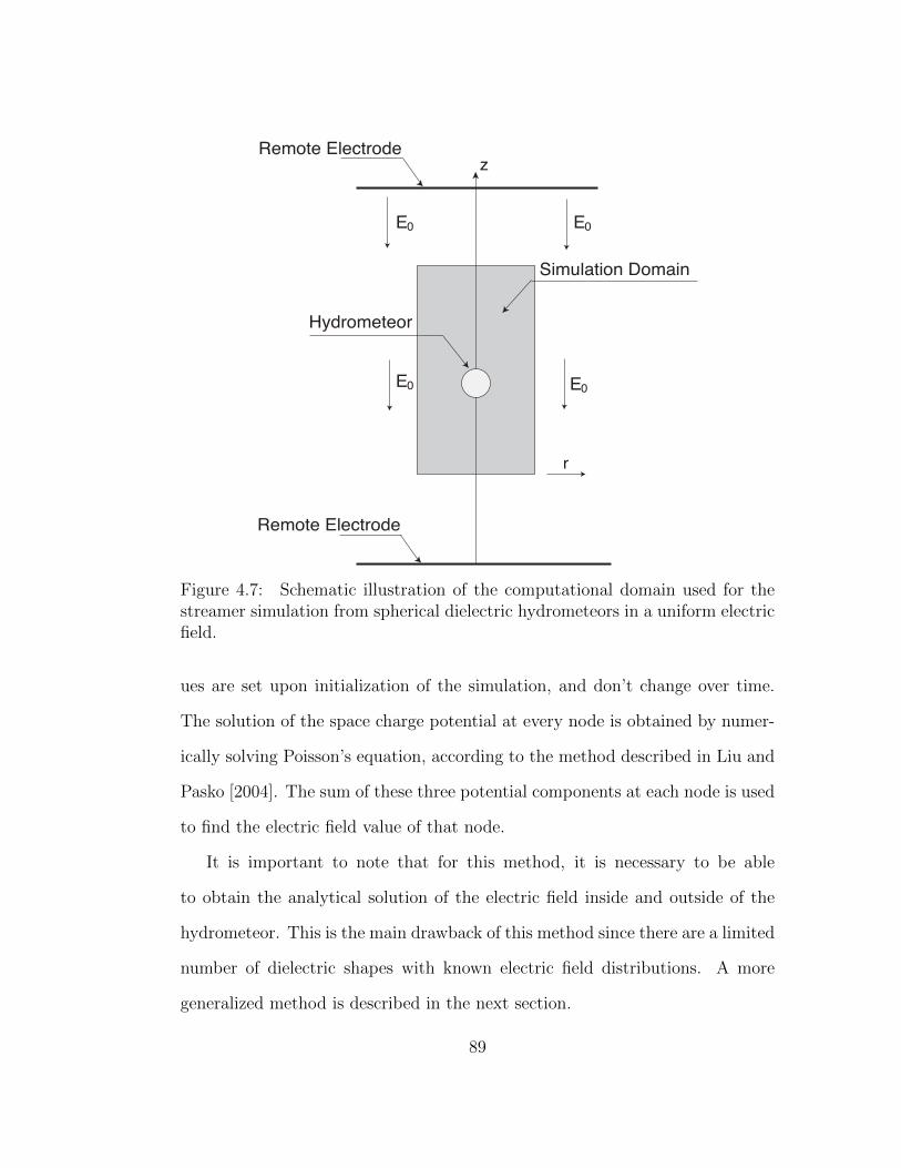
Simulation Domain
Hydrometeor
z
E0 E0
E0 E0
Remote Electrode
Remote Electrode
r
Figure 4.7: Schematic illustration of the computational domain used for thestreamer simulation from spherical dielectric hydrometeors in a uniform electricfield.
ues are set upon initialization of the simulation, and don’t change over time.
The solution of the space charge potential at every node is obtained by numer-
ically solving Poisson’s equation, according to the method described in Liu and
Pasko [2004]. The sum of these three potential components at each node is used
to find the electric field value of that node.
It is important to note that for this method, it is necessary to be able
to obtain the analytical solution of the electric field inside and outside of the
hydrometeor. This is the main drawback of this method since there are a limited
number of dielectric shapes with known electric field distributions. A more
generalized method is described in the next section.
89
4.6.2 Variable Polarization: Liquid Water Filaments
The case of a dielectric hydrometeor with variable polarization is more complex
than the constant polarization. In this situation, the electric polarization inside
the dielectric hydrometeor changes as a response to the varying space charge
density in the system. In order to solve for the electric potential inside the
dielectric, proper boundary conditions must be implemented at the dielectric-
air interface. The two general electrostatic boundary conditions that must be
imposed on this boundary are as follows:
Dn1 −Dn2 = σf (4.4)
Et1 − Et2 = 0 (4.5)
where the medium inside the dielectric is denoted as 1, and the air outside
is denoted as medium 2; n refers to the normal to the plane, and t refers to
tangential; Dn is the normal component of the displacement vector ~D, and
Et is the tangential component of ~E. These two conditions imply that at the
interface, the normal component of the displacement vector is discontinuous
if free charge is present on the surface, and the tangential component of the
electric field vector is continuous. For our simulations, there are no free surface
charges deliberately placed on the surface of the dielectric. In this case, the
right hand side of Equation 4.4 will also be equal to zero, meaning that both
components are continuous.
In order to properly enforce the boundary conditions on the curved bound-
ary, we utilize a boundary condition capturing method proposed by Liu et al.
90
[2000] for solving Poisson’s equation on irregular boundaries. This method has
been presented specifically for solving Poisson’s equation where the solution
may be discontinuous across an immersed boundary. A major advantage of this
method is that it has been developed so that the coefficient matrix associated
with the linear system produced by discretization of Poisson’s equation will
keep its standard format used in the absence of immersed boundaries. In other
words, any numerical method that has been utilized to solve Poisson’s equation
on a standard domain without an immersed boundary, can still be used. This
greatly simplifies the numerical implementation of this technique.
This method is based on a similar approach as the Ghost Fluid Method
(GFM) [Fedkiw et al., 1999]. The generalized GFM captures the appropriate
boundary conditions at an interface, without explicitly enforcing them. In-
stead, the method creates an artificial fluid which implicitly induces the proper
conditions at the interface. Simply put, the boundary conditions will be sat-
isfied without actually enforcing them on the physical curved/irregular shaped
boundary. A detailed description of the implementation of this method in our
streamer model will be given below.
Assume a simulation setup similar to that shown in Figure 4.8. We want to
solve for the electric potential V, from Poisson’s equation:
∇.(ε∇V ) = −ρ, (4.6)
where ε is the permittivity; and ρ is the free charge density. In cylindrical
coordinates, the two dimensional Poisson’s equation can be written as follows:
91
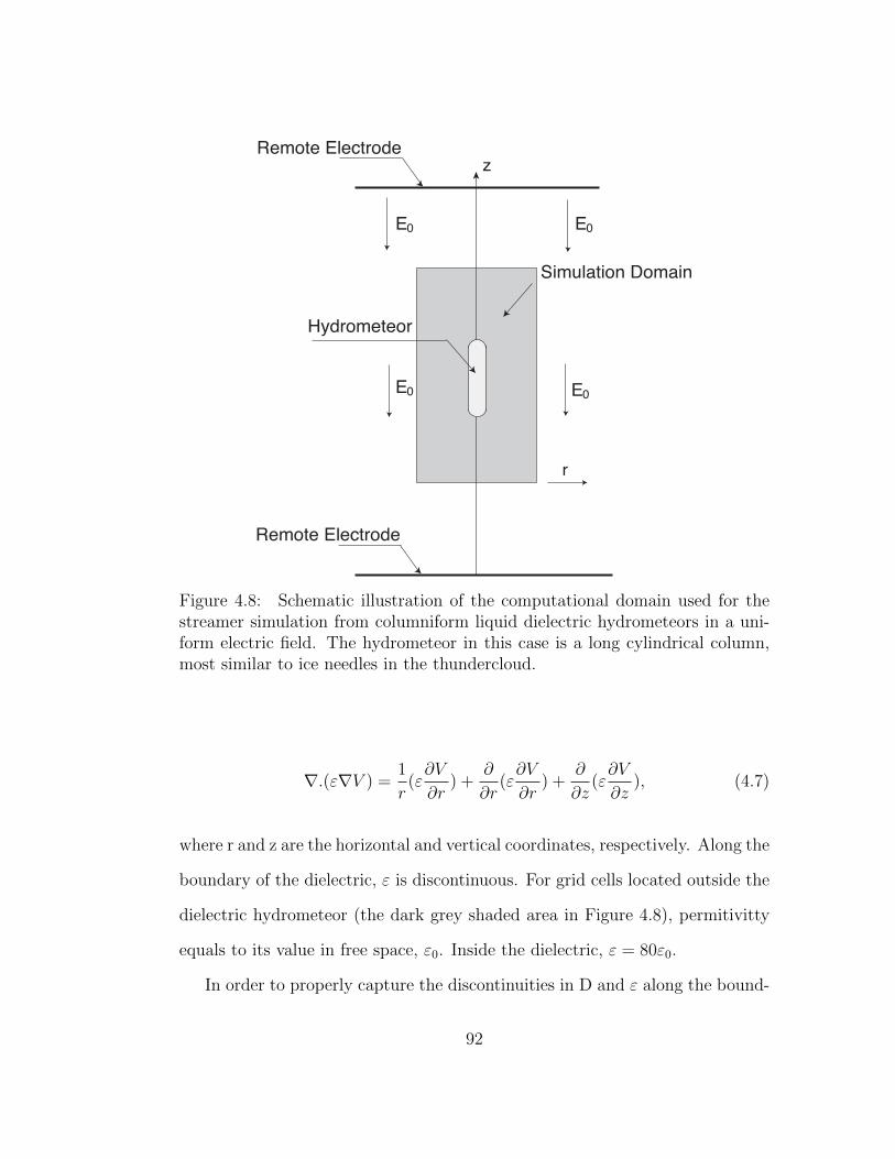
Simulation Domain
Hydrometeor
z
E0 E0
E0 E0
Remote Electrode
Remote Electrode
r
Figure 4.8: Schematic illustration of the computational domain used for thestreamer simulation from columniform liquid dielectric hydrometeors in a uni-form electric field. The hydrometeor in this case is a long cylindrical column,most similar to ice needles in the thundercloud.
∇.(ε∇V ) =1
r(ε∂V
∂r) +
∂
∂r(ε∂V
∂r) +
∂
∂z(ε∂V
∂z), (4.7)
where r and z are the horizontal and vertical coordinates, respectively. Along the
boundary of the dielectric, ε is discontinuous. For grid cells located outside the
dielectric hydrometeor (the dark grey shaded area in Figure 4.8), permitivitty
equals to its value in free space, ε0. Inside the dielectric, ε = 80ε0.
In order to properly capture the discontinuities in D and ε along the bound-
92
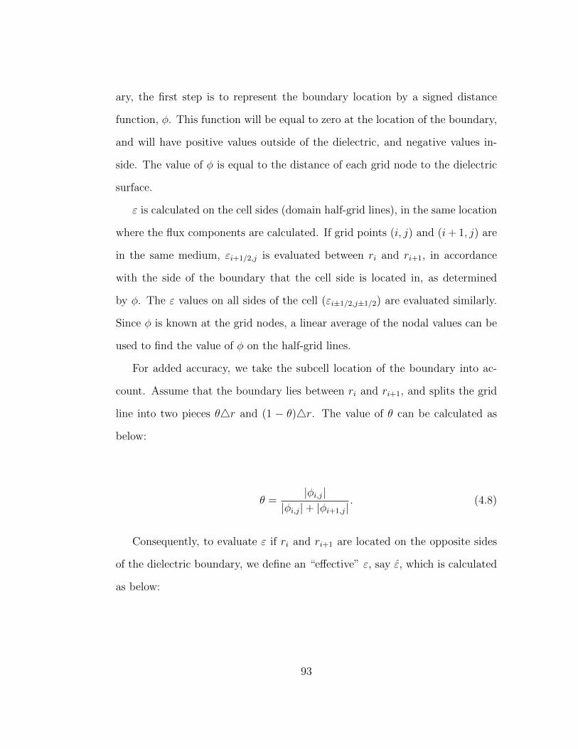
ary, the first step is to represent the boundary location by a signed distance
function, φ. This function will be equal to zero at the location of the boundary,
and will have positive values outside of the dielectric, and negative values in-
side. The value of φ is equal to the distance of each grid node to the dielectric
surface.
ε is calculated on the cell sides (domain half-grid lines), in the same location
where the flux components are calculated. If grid points (i, j) and (i+ 1, j) are
in the same medium, εi+1/2,j is evaluated between ri and ri+1, in accordance
with the side of the boundary that the cell side is located in, as determined
by φ. The ε values on all sides of the cell (εi±1/2,j±1/2) are evaluated similarly.
Since φ is known at the grid nodes, a linear average of the nodal values can be
used to find the value of φ on the half-grid lines.
For added accuracy, we take the subcell location of the boundary into ac-
count. Assume that the boundary lies between ri and ri+1, and splits the grid
line into two pieces θ4r and (1 − θ)4r. The value of θ can be calculated as
below:
θ =|φi,j|
|φi,j|+ |φi+1,j|. (4.8)
Consequently, to evaluate ε if ri and ri+1 are located on the opposite sides
of the dielectric boundary, we define an “effective” ε, say ε, which is calculated
as below:
93
ε =εi+1,jεi,j
εi+1,jθ + εi+1,j(1− θ). (4.9)
With these definitions, we can discretize the right hand side of Equation 4.7
as follows:
RHS =1
4r[εi+1/2,j(
Vi+1,j − Vi,j4r
)− εi−1/2,j(Vi,j − Vi−1,j
4r)]+
1
4z[εi,j+1/2(
Vi,j+1 − Vi,j4z
)− εi,j−1/2(Vi,j − Vi,j−1
4z)]+
1
2ri,j[εi+1/2,j(
Vi+1,j − Vi,j4r
) + εi−1/2,j(Vi,j − Vi−1,j
4r)]. (4.10)
Substituting Equations 4.8, and 4.9 into Equation 4.10, finalizes the imple-
mentation of the boundary condition capturing method proposed by Liu et al.
[2000]. It is important to note that the last term in Equation 4.10 has an ri,j
term in the denominator, which will be problematic for the grid points along
the symmetry axis of the domain, where ri,j = 0. To overcome this problem, we
use L’Hopital’s rule to evaluate this indeterminate term. As a result, Equation
4.10 will be written as below, for the grid points along the symmetry axis only:
RHS =2
4r[εi+1/2,j(
Vi+1,j − Vi,j4r
)− εi−1/2,j(Vi,j − Vi−1,j
4r)]+
1
4z[εi,j+1/2(
Vi,j+1 − Vi,j4z
)− εi,j−1/2(Vi,j − Vi,j−1
4z)]. (4.11)
The resulting linear equations in 4.10 and 4.11 can be transformed into a
94
system of linear equations, and solved using the SOR method. The boundary
capturing method used here has the great advantage of simplicity of imple-
mentation. The algorithm described above, can be applied to any dielectric
hydrometeor shape, whether the analytical solution of the electric field is avail-
able or not.
4.7 Modeling Results from the Dielectric Hy-
drometeor
In this section, we present streamer simulation results from each of the two
states of the dielectric hydrometeor presented above.
4.7.1 Solid Ice Particles
Figure 4.9 shows cross-sectional views of distributions of electron density and
electric field of a streamer that has successfully formed from an isolated spherical
dielectric hydrometeor. The hydrometeor is placed in an ambient electric field
value of E0 = 0.9Ek, at 7 km altitude. The radius of the hydrometeor is equal to
3.1 mm, consistent with typical hydrometeor dimensions, and an initial plasma
cloud is present to provide seed electrons. The plasma cloud has a Gaussian
distribution with σ = 0.22 mm and peak density = 1× 10¹⁷ m−3.
Figure 4.10 shows profiles of electron density and electric field along the
symmetry axis of the streamer, at different moments of time. To avoid confusion,
the profiles show the positive tip of the hydrometeor only. The direction of
propagation of the streamer in each profile is from right to left. From these
figures, the streamer channel density value is about 5 × 10¹⁹ m−3, and the
95
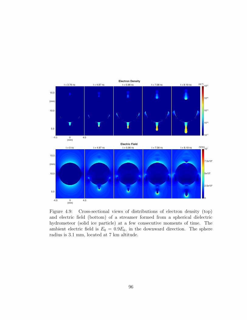
t = 8.19 ns
1017
1018
1019
1020
1021(m-3)t = 7.08 nst = 5.98 nst = 4.87 nst = 3.76 ns
-4.0 0 4.0
15.0
10.0
5.0
(mm)
(mm)
Electron Density
Electric Field
t = 8.19 ns
0
2.5x10⁶
5x10⁶
7.5x10⁶
107(V/m)t = 7.08 nst = 5.98 nst = 4.87 nst = 0 ns
-4.0 0 4.0
15.0
10.0
5.0
(mm)
(mm)
Figure 4.9: Cross-sectional views of distributions of electron density (top)and electric field (bottom) of a streamer formed from a spherical dielectrichydrometeor (solid ice particle) at a few consecutive moments of time. Theambient electric field is E0 = 0.9Ek, in the downward direction. The sphereradius is 3.1 mm, located at 7 km altitude.
96
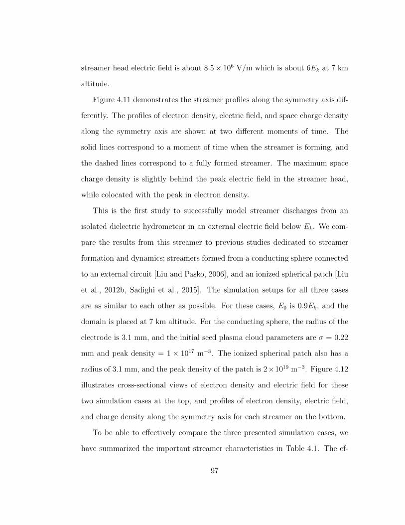
streamer head electric field is about 8.5× 10⁶ V/m which is about 6Ek at 7 km
altitude.
Figure 4.11 demonstrates the streamer profiles along the symmetry axis dif-
ferently. The profiles of electron density, electric field, and space charge density
along the symmetry axis are shown at two different moments of time. The
solid lines correspond to a moment of time when the streamer is forming, and
the dashed lines correspond to a fully formed streamer. The maximum space
charge density is slightly behind the peak electric field in the streamer head,
while colocated with the peak in electron density.
This is the first study to successfully model streamer discharges from an
isolated dielectric hydrometeor in an external electric field below Ek. We com-
pare the results from this streamer to previous studies dedicated to streamer
formation and dynamics; streamers formed from a conducting sphere connected
to an external circuit [Liu and Pasko, 2006], and an ionized spherical patch [Liu
et al., 2012b, Sadighi et al., 2015]. The simulation setups for all three cases
are as similar to each other as possible. For these cases, E0 is 0.9Ek, and the
domain is placed at 7 km altitude. For the conducting sphere, the radius of the
electrode is 3.1 mm, and the initial seed plasma cloud parameters are σ = 0.22
mm and peak density = 1 × 10¹⁷ m−3. The ionized spherical patch also has a
radius of 3.1 mm, and the peak density of the patch is 2×10¹⁹ m−3. Figure 4.12
illustrates cross-sectional views of electron density and electric field for these
two simulation cases at the top, and profiles of electron density, electric field,
and charge density along the symmetry axis for each streamer on the bottom.
To be able to effectively compare the three presented simulation cases, we
have summarized the important streamer characteristics in Table 4.1. The ef-
97
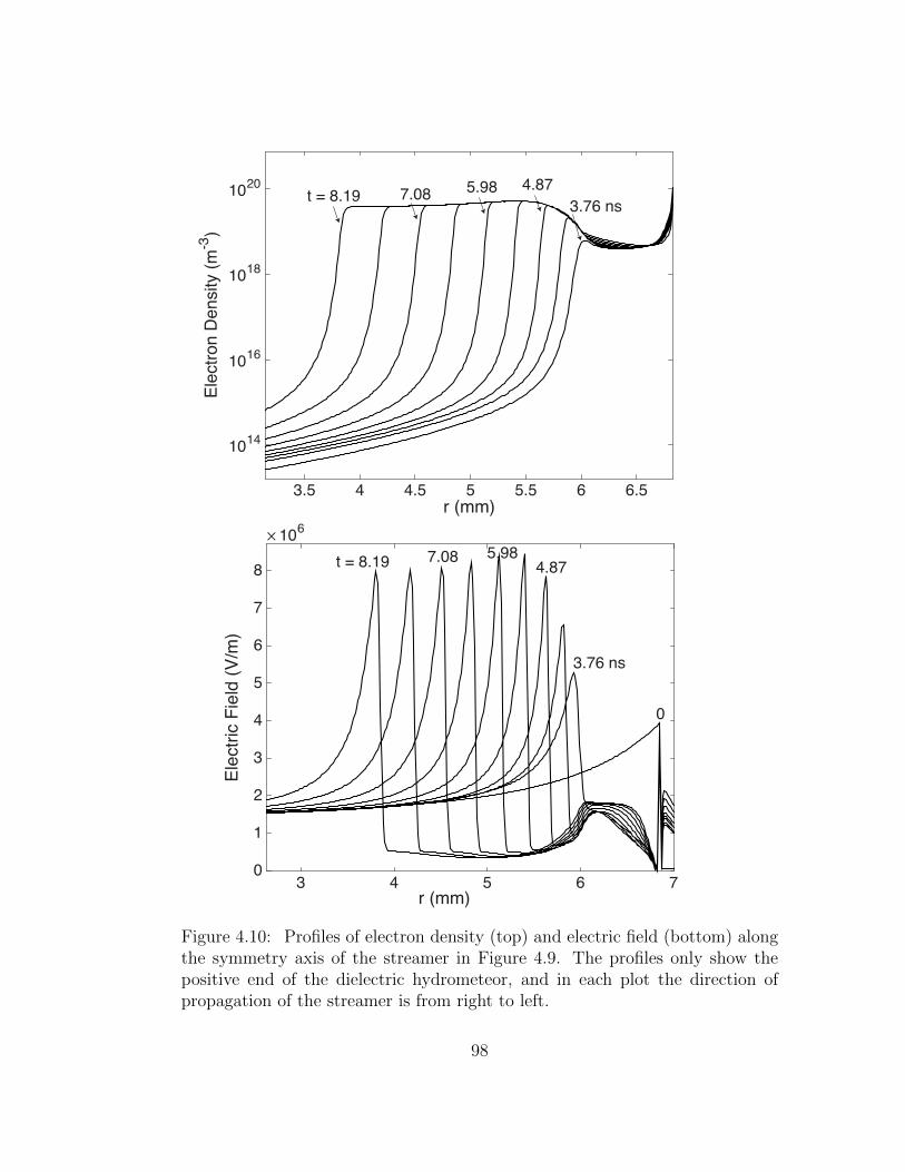
r (mm)3 4 5 6 7
Ele
ctr
ic F
ield
(V
/m)
× 106
0
1
2
3
4
5
6
7
8t = 8.19 7.08 5.98
4.87
3.76 ns
0
r (mm)3.5 4 4.5 5 5.5 6 6.5
Ele
ctr
on
De
nsity (
m-3
)
1014
1016
1018
1020
t = 8.19 7.08 5.98 4.87
3.76 ns
Figure 4.10: Profiles of electron density (top) and electric field (bottom) alongthe symmetry axis of the streamer in Figure 4.9. The profiles only show thepositive end of the dielectric hydrometeor, and in each plot the direction ofpropagation of the streamer is from right to left.
98
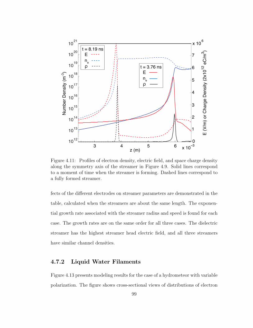
3 4 5 6 x 10⁻³
z (m)
1
2
3
4
5
6
7
x 106
E (
V/m
) o
r C
ha
rge
De
nsity (
2x1
01
2 e
C/m
3)
01012
1013
1014
1015
1016
1017
1018
1019
1020
1021
Nu
mb
er
De
nsity (
m-3
)
t = 8.19 ns
E
ne
ρ t = 3.76 ns
E
ne
ρ
Figure 4.11: Profiles of electron density, electric field, and space charge densityalong the symmetry axis of the streamer in Figure 4.9. Solid lines correspondto a moment of time when the streamer is forming. Dashed lines correspond toa fully formed streamer.
fects of the different electrodes on streamer parameters are demonstrated in the
table, calculated when the streamers are about the same length. The exponen-
tial growth rate associated with the streamer radius and speed is found for each
case. The growth rates are on the same order for all three cases. The dielectric
streamer has the highest streamer head electric field, and all three streamers
have similar channel densities.
4.7.2 Liquid Water Filaments
Figure 4.13 presents modeling results for the case of a hydrometeor with variable
polarization. The figure shows cross-sectional views of distributions of electron
99
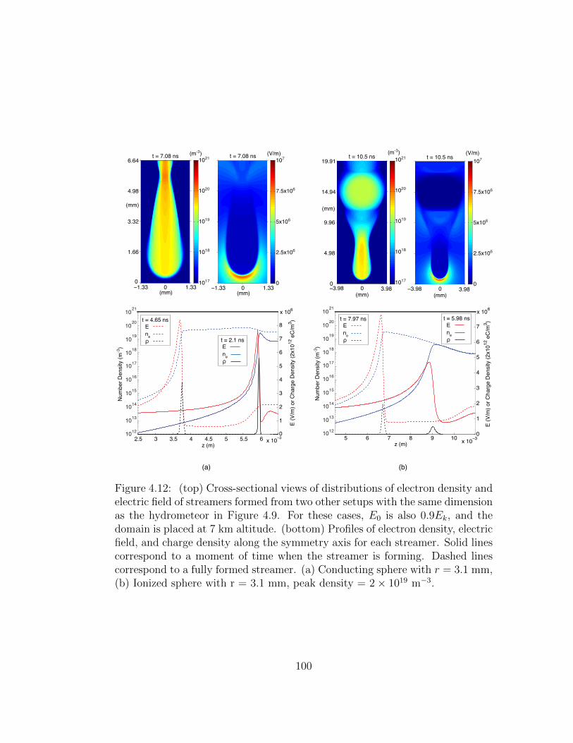
t = 10.5 ns
−3.98 0 3.98
19.91
14.94
9.96
4.98
0 1017
1018
1019
1020
1021
(mm)
(m-3)
(mm)
0
2.5x10⁶
5x10⁶
7.5x10⁶
107t = 10.5 ns
−3.98 0 3.98
(V/m)
(mm)
t = 7.08 ns
−1.33 0 1.33
6.64
4.98
3.32
1.66
0 1017
1018
1019
1020
1021
(mm)
(mm)
(m-3)
0
2.5x10⁶
5x10⁶
7.5x10⁶
107
−1.33 0 1.33(mm)
t = 7.08 ns (V/m)
5 6 7 8 9 10x 10
−3
z (m)
0
1
2
3
4
5
6
7
x 106
E (
V/m
) o
r C
ha
rge
De
nsity (
2x1
01
2 e
C/m
3)
1012
1013
1014
1015
1016
1017
1018
1019
1020
1021
Nu
mb
er
De
nsity (
m-3
)t = 7.97 ns
E
ne
ρ
t = 5.98 ns
E
ne
ρ
2.5 3 3.5 4 4.5 5 5.5 6 x 10⁻³
1012
1013
1014
1015
1016
1017
1018
1019
1020
1021
z (m)
Nu
mb
er
De
nsity (
m-3
)
0
1
2
3
4
5
6
7
8
x 106
E (
V/m
) o
r C
ha
rge
De
nsity (
2x1
01
2 e
C/m
3)
t = 2.1 ns
E
ne
ρ
t = 4.65 ns
E
ne
ρ
(a) (b)
Figure 4.12: (top) Cross-sectional views of distributions of electron density andelectric field of streamers formed from two other setups with the same dimensionas the hydrometeor in Figure 4.9. For these cases, E0 is also 0.9Ek, and thedomain is placed at 7 km altitude. (bottom) Profiles of electron density, electricfield, and charge density along the symmetry axis for each streamer. Solid linescorrespond to a moment of time when the streamer is forming. Dashed linescorrespond to a fully formed streamer. (a) Conducting sphere with r = 3.1 mm,(b) Ionized sphere with r = 3.1 mm, peak density = 2× 10¹⁹ m−3.
100
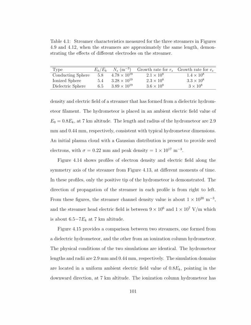
Table 4.1: Streamer characteristics measured for the three streamers in Figures4.9 and 4.12, when the streamers are approximately the same length, demon-strating the effects of different electrodes on the streamer.
Type Eh/Ek Ns (m−3) Growth rate for rs Growth rate for vsConducting Sphere 5.8 4.78× 10¹⁹ 2.1× 10⁸ 1.4× 10⁸
Ionized Sphere 5.4 3.28× 10¹⁹ 2.3× 10⁸ 3.3× 10⁸
Dielectric Sphere 6.5 3.89× 10¹⁹ 3.6× 10⁸ 3× 10⁸
density and electric field of a streamer that has formed from a dielectric hydrom-
eteor filament. The hydrometeor is placed in an ambient electric field value of
E0 = 0.8Ek, at 7 km altitude. The length and radius of the hydrometeor are 2.9
mm and 0.44 mm, respectively, consistent with typical hydrometeor dimensions.
An initial plasma cloud with a Gaussian distribution is present to provide seed
electrons, with σ = 0.22 mm and peak density = 1× 10¹⁷ m−3.
Figure 4.14 shows profiles of electron density and electric field along the
symmetry axis of the streamer from Figure 4.13, at different moments of time.
In these profiles, only the positive tip of the hydrometeor is demonstrated. The
direction of propagation of the streamer in each profile is from right to left.
From these figures, the streamer channel density value is about 1 × 10²⁰ m−3,
and the streamer head electric field is between 9× 10⁶ and 1× 10⁷ V/m which
is about 6.5−7Ek at 7 km altitude.
Figure 4.15 provides a comparison between two streamers, one formed from
a dielectric hydrometeor, and the other from an ionization column hydrometeor.
The physical conditions of the two simulations are identical. The hydrometeor
lengths and radii are 2.9 mm and 0.44 mm, respectively. The simulation domains
are located in a uniform ambient electric field value of 0.8Ek, pointing in the
downward direction, at 7 km altitude. The ionization column hydrometeor has
101
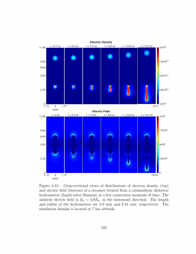
t = 5.7 ns
-1.77 0 1.77
11.06
8.30
5.53
2.76
0
(mm)
(mm)
t = 6.4 ns t = 7.3 ns t = 8.6 ns t = 10.8 ns t = 14.2 ns
1x10¹⁴
5.6x10¹⁵
3.2x10¹⁷
1.8x10¹⁹
1x10²¹
(m-3)
Electron Density
Electric Field
t = 0 ns
-1.77 0 1.77
11.06
8.30
5.53
2.76
0
(mm)
(mm)
t = 6.4 ns t = 7.3 ns t = 8.6 ns t = 10.8 ns t = 14.2 ns
0
2.5x10⁶
5x10⁶
7.5x10⁶
1x10⁷
(V/m)
Figure 4.13: Cross-sectional views of distributions of electron density (top)and electric field (bottom) of a streamer formed from a columniform dielectrichydrometeor (liquid water filament) at a few consecutive moments of time. Theambient electric field is E0 = 0.8Ek, in the downward direction. The lengthand radius of the hydrometeor are 2.9 mm and 0.44 mm, respectively. Thesimulation domain is located at 7 km altitude.
102
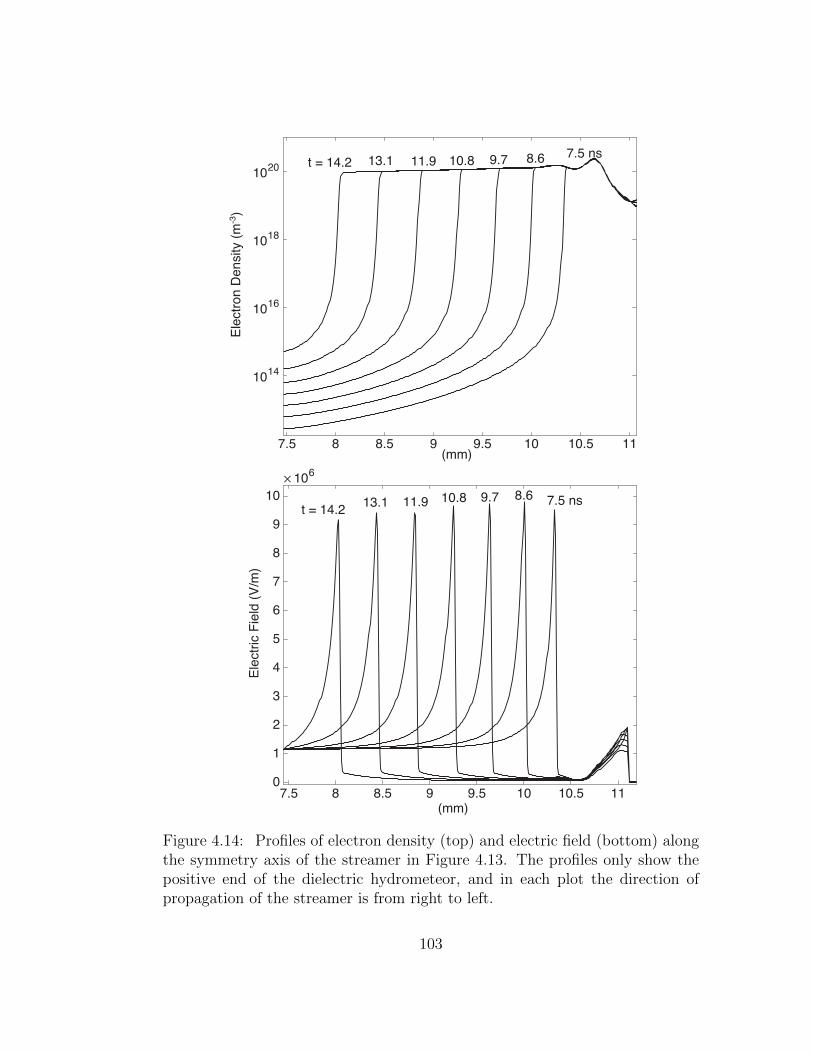
(mm)
1014
1016
1018
1020
Ele
ctr
on
De
nsity (
m-3
)
7.5 8 8.5 9 9.5 10 10.5 11
t = 14.27.5 ns
9.7 8.610.811.913.1
7.5 8 8.5 9 9.5 10 10.5 11
× 106
0
1
2
3
4
5
6
7
8
9
10
(mm)
Ele
ctr
ic F
ield
(V
/m)
t = 14.27.5 ns9.7 8.610.811.913.1
Figure 4.14: Profiles of electron density (top) and electric field (bottom) alongthe symmetry axis of the streamer in Figure 4.13. The profiles only show thepositive end of the dielectric hydrometeor, and in each plot the direction ofpropagation of the streamer is from right to left.
103
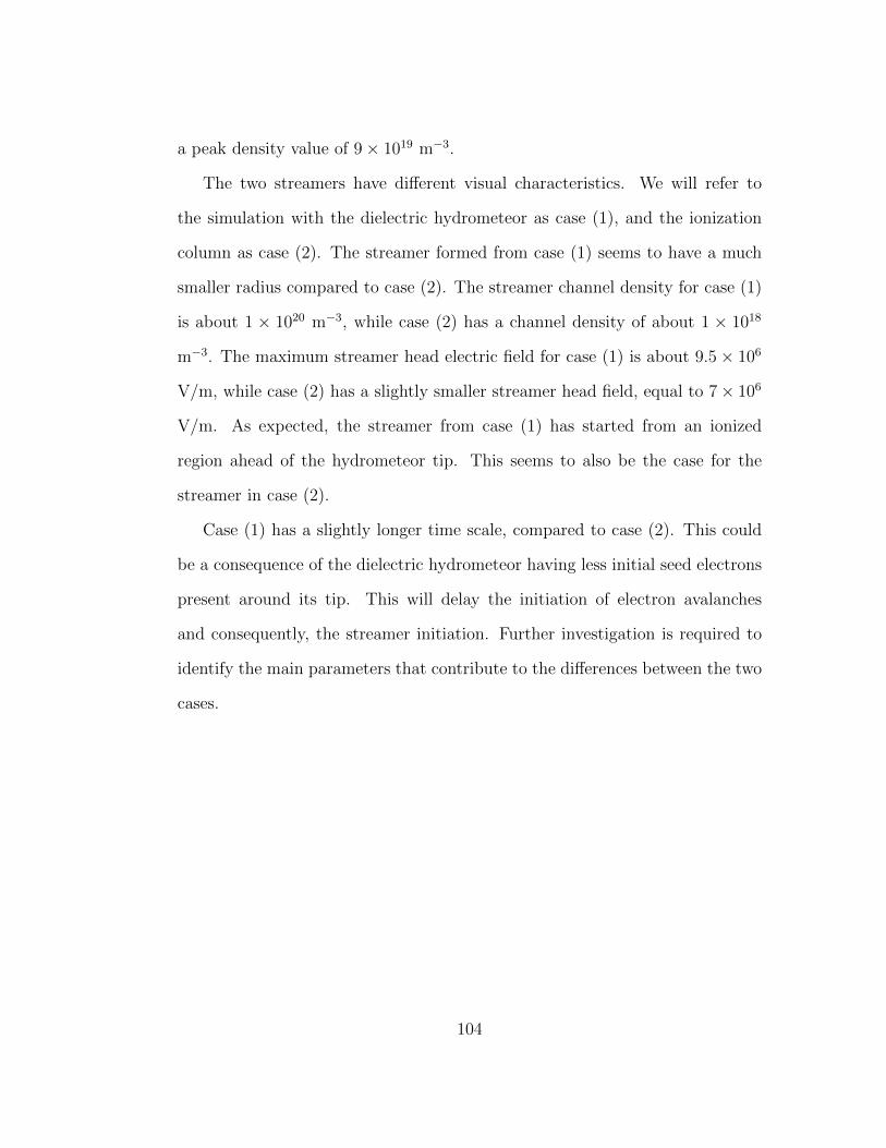
a peak density value of 9× 10¹⁹ m−3.
The two streamers have different visual characteristics. We will refer to
the simulation with the dielectric hydrometeor as case (1), and the ionization
column as case (2). The streamer formed from case (1) seems to have a much
smaller radius compared to case (2). The streamer channel density for case (1)
is about 1 × 10²⁰ m−3, while case (2) has a channel density of about 1 × 10¹⁸
m−3. The maximum streamer head electric field for case (1) is about 9.5× 10⁶
V/m, while case (2) has a slightly smaller streamer head field, equal to 7× 10⁶
V/m. As expected, the streamer from case (1) has started from an ionized
region ahead of the hydrometeor tip. This seems to also be the case for the
streamer in case (2).
Case (1) has a slightly longer time scale, compared to case (2). This could
be a consequence of the dielectric hydrometeor having less initial seed electrons
present around its tip. This will delay the initiation of electron avalanches
and consequently, the streamer initiation. Further investigation is required to
identify the main parameters that contribute to the differences between the two
cases.
104
t = 6.6 ns
-1.77 0 1.77
11.06
8.30
5.53
2.76
0
(mm)
(mm)
1x10¹⁷
1x10¹⁸
1x10²¹
(m-3)
1x10¹⁹
1x10²⁰
-1.77 0 1.77
11.06
8.30
5.53
2.76
0
(mm)
(mm)
0
2.5x10⁶
5x10⁶
7.5x10⁶
1x10⁷
(V/m)t = 6.6 ns
Ionization Column Hydrometeor
-1.77 0 1.77
11.06
8.30
5.53
2.76
0
(mm)
(mm)
t = 14.8 ns(m
-3)
1x10¹⁷
18
1x10²¹
1x10
19
20
1x10
1x10
-1.77 0 1.77
11.06
8.30
5.53
2.76
0
(mm)
(mm)
t = 14.8 ns
0
2.5x10⁶
5x10⁶
7.5x10⁶
1x10⁷
(V/m)
Dielectric Hydrometeor
Figure 4.15: Cross-sectional views of electron density and electric field ofstreamers formed from: (top) a dielectric hydrometeor; case (1), and (bottom)an ionization column hydrometeor; case (2).
105
Chapter 5
Summary and Future Work
5.1 Summary of Results
How lightning originates inside thunderclouds and propagates through air is
a longstanding fundamental problem in the field of atmospheric electricity.
Lightning researchers have been trying to answer this question since Benjamin
Franklin discovered the electrical nature of lightning through his famous kite
experiment [e.g., Rakov and Uman, 2003, p. 121, and references cited therein].
The theoretical efforts of this dissertation research has aimed to advance the
current knowledge of lightning initiation. The first step in improving our under-
standing of lightning initiation is to study the precursors of lightning leaders,
streamers. We have focused our efforts on studying streamer initiation and prop-
agation from thundercloud hydrometeors and have established that streamers
can be initiated from thundercloud hydrometeors in the maximum thundercloud
electric field measured so far, which is well below the conventional breakdown
threshold field Ek.
106
For the first part of this study, we have further investigated the idea proposed
by Liu et al. [2012b] to study streamers from ionization column hydrometeors in
thundercloud conditions. According to our simulation results, positive stream-
ers can be initiated from columniform hydrometeors subject to the maximum
observed thundercloud electric fields of∼ 0.3Ek. We have performed simulations
for ambient electric field values of 0.5Ek at thundercloud altitudes, and obtained
successful streamer formation, confirming the work of Liu et al. [2012b]. Reduc-
ing the ambient electric field to as low as 0.3Ek affects the streamer’s ability to
propagate stably. In this case the streamer will either not form, or branch during
initiation. The branching of the streamer interrupts the stable streamer prop-
agation and changes the dynamics of the streamer. According to our results,
introducing a proper background ionization distribution stabilizes the initiation
and propagation of the streamer. We have investigated the streamer branching
behavior and characteristics, and a theory to explain the mechanism of this
phenomenon has been formulated and tested.
In order to verify whether an ionization column is a proper representation of
a dielectric hydrometeor, for the second part of this dissertation we modify the
streamer discharge model to accommodate an isolated dielectric particle repre-
senting the hydrometeor inside the computational region. Since the governing
equations of the plasma discharge model are discretized on a uniform rectangu-
lar grid, the boundary cells do not conform to the shape of the dielectric. We
utilize a boundary-cut cell method proposed by Ye et al. [1999] to handle these
cut cells, and properly evaluate the corresponding fluxes. A boundary condi-
tion capturing method by Liu et al. [2000] has been used to properly enforce
the electrostatic boundary conditions on the dielectric hydrometeor. This model
107
enables us to accurately simulate the discharges around dielectric hydrometeors
with various shapes and physical states. Streamer discharge results obtained
from the dielectric hydrometeor have been presented and compared with the
results obtained from the first part of this work.
5.2 Implications to Lightning Initiation
The modeling study presented here has direct implications to lightning initia-
tion, since streamers are known to be the precursors of lightning leaders. The
obtained results demonstrate that hydrometeors present in measured thunder-
cloud electric field values can give rise to streamer discharges. This is the first
detailed theoretical modeling study that has been able to confirm the experi-
mental work previously done on this topic [e.g., Crabb and Latham, 1974, Grif-
fiths and Latham, 1974, Petersen et al., 2006]. The maximum of the observed
thundercloud electric field values hundreds of meters away from the lightning
initiation point just before lightning discharges are typically between 300 and
450 kV/m (at ground pressure) [Marshall et al., 1995], while higher values as
large as 929 kV/m (at ground pressure) have also been measured [Stolzenburg
et al., 2007]. The minimum ambient electric field value used in this study is
equivalent to 960 kV/m at ground pressure. For this electric field, the initiation
and stable propagation of the streamer has been shown to depend on the amount
and distribution of background ionization present inside the cloud. Confirma-
tion of streamer formation from hydrometeors inside thundercloud electric fields
positively impacts lightning initiation studies.
This study also has implications to lightning related phenomena such as the
108
relativistic feedback discharges that are thought to produce Terrestrial Gamma-
ray Flashes (TGFs) [Dwyer, 2012, Dwyer et al., 2012, Liu and Dwyer, 2013].
Terrestrial gamma-ray flashes are bursts of extremely high energy radiation
coming from thunderclouds and have been observed from space [e.g., Fishman
et al., 1994] and from ground [Dwyer et al., 2012]. One theory to explain
TGF production from thunderclouds is relativistic feedback discharges [Dwyer,
2012, Liu and Dwyer, 2013]. According to Dwyer [2012] and Liu and Dwyer
[2013], TGF pulses can be produced naturally by the relativistic feedback dis-
charge that develops in thundercloud electric fields. These studies introduced
a self-propagating discharge resulting from the relativistic feedback discharge
mechanism, called the relativistic feedback streamer. The relativistic feedback
streamer tends to propagate unstably, and the electric field in the streamer
head continually increases. This head field can reach up to one-third to one-
half of the conventional breakdown threshold field, raising the possibility that
if a hydrometeor is present inside the relativistic feedback streamer head field,
a conventional streamer is able to form.
From our study, for electric field values lower than 0.3Ek, it is unlikely that
the conventional streamer is initiated from realistic hydrometeors. At an early
stage of the relativistic feedback streamer, when the peak electric field in the
head is smaller than 0.3Ek, conventional streamer activity may therefore be
ignored. Figures 6a and 10 from the study by Liu and Dwyer [2013] present
axial profiles of the electric field of a relativistic feedback streamer propagating
in a uniform and nonuniform thundercloud electric field, respectively. From
their Figure 6a, the relativistic feedback streamer propagates for about 12 ms
before the electric field at the head exceeds 0.3Ek. During this time, the first
109
two TGF pulses have already been produced (Figure 7 in Liu and Dwyer [2013]).
The relativistic feedback streamer propagating in a nonuniform field (Figure 10
in Liu and Dwyer [2013]) demonstrates a similar behavior. The electric field in
the head of the feedback streamer exceeds 0.3Ek after about 15 ms, during which
at least three TGF pulses have been produced. This means that the relativistic
feedback discharge streamer can produce TGF pulses before any conventional
streamers might be initiated from positive hydrometeors.
Based on what has been demonstrated here, when the electric field in the
relativistic feedback streamer head reaches and exceeds 0.3Ek, with the presence
of hydrometeors around the relativistic feedback streamer head, it is possible
that conventional streamers may form. Liu and Dwyer [2013] have estimated
the residence time of the high electric field of the relativistic feedback streamer
to be 200 µs, which is sufficient time for polarization of water or ice hydrome-
teors. Therefore, it may be expected that bursts of streamers are produced in
the later stage of the relativistic feedback discharge. The importance of these
conventional streamer discharges in the dynamics of the feedback streamer has
yet to be investigated.
5.3 Suggestions for Future Work
The ultimate objective of the project we have started in this dissertation re-
search is to improve our understanding of how lightning is initiated in the thun-
dercloud and how it can propagate such long distances through air. This study
offers solid results for continuing this path to improve the knowledge of light-
ning. There are three critical steps in the lightning initiation and propagation
110
problem: the initiation and propagation of streamers in observed thundercloud
electric fields, the transition of these streamers to bright, hot, and highly con-
ductive leaders, and the propagation of leaders.
The results of this study have shown that streamers can be initiated from
thundercloud hydrometeors in maximum thundercloud electric fields. The next
step for continuing this research would be to understand how the streamer-to-
leader transition occurs. Whether the streamers originating from thundercloud
hydrometeors will be able to generate a leader is still unknown. There are a
number of scientific questions that must be resolved in this area. For example,
what are the effects of Joule heating in the streamer channels originating from
thundercloud hydrometeors? What are the thundercloud conditions that the
streamer-to-leader transition depends on? We believe that the contributing
results of this dissertation research will have a significant impact on following
this path to understanding lightning.
111
Bibliography
M. Arrayas, U. Ebert, and W. Hundsdorfer. Spontaneous branching of anode-
directed streamers between planar electrodes. Phys. Rev. Lett., 88:174502(R),
2002. doi: 10.1103/PhysRevLett.88.174502.
L. P. Babich, I. M. Kutsyk, E. N. Donskoy, and A. Y. Kudryavtsev. New
data on space and time scales of relativistic runaway electron avalanche for
thunderstorm environment: Monte carlo calculations. Physics Letters A, 245
(5):460–470, 1998.
L. P. Babich, E. N. Donskoy, I. M. Kutsyk, A. Y. Kudryavtsev, R. A. Roussel-
Dupre, B. N. Shamraev, and E. M. D. Symbalisty. Comparison of relativistic
runaway electron avalanche rates obtained from monte carlo simulations and
kinetic equation solution. Plasma Science, IEEE Transactions on, 29(3):430–
438, 2001.
L. P. Babich, E. I. Bochkov, J. R. Dwyer, and I. M. Kutsyk. Numerical simula-
tions of local thundercloud field enhancements caused by runaway avalanches
seeded by cosmic rays and their role in lightning initiation. J. Geophys. Res.,
117(16):A09316, 2012. doi: 10.1029/2012JA017799.
M. G. Bateman, T. C. Marshall, M. Stolzenburg, and W. D. Rust. Precipitation
112
charge and size measurements inside a New Mexico mountain thunderstorm.
J. Geophys. Res., 104(D8):9643–9653, 1999.
E. M. Bazelyan and Y. P. Raizer. Spark Discharge. Chemical Rubber Company
Press, New York, NY, 1998.
A. M. Blyth, H. J. Christian, and J. Latham. Corona emission thresholds for
three types of hydrometeor interaction in thunderclouds. J. Geophys. Res.,
103:13975–13978, 1998. doi: 10.1029/97JD02554.
A. Bourdon, V. P. Pasko, N. Y. Liu, S. Celestin, P. Segur, and E. Marode. Ef-
ficient models for photoionization produced by non-thermal gas discharges in
air based on radiative transfer and the Helmholtz equations. Plasma Sources
Sci. Technol., 16:656–678, 2007. doi: 10.1088/0963-0252/16/3/026.
J. Chen and J. H. Davidson. Electron density and energy distributions in the
positive DC corona: interpretation for corona-enhanced chemical reactions.
Plasma Chemistry and Plasma Processing, 22(2):199–224, 2002.
J. Chen and J. H. Davidson. Model of the negative dc corona plasma: com-
parison to the positive dc corona plasma. Plasma Chemistry and Plasma
Processing, 23(1):83–102, 2003.
C. Chiu and J. D. Klett. Convective electrification of clouds. J. Geophys. Res.,
81(6):1111–1124, 1976.
V. Cooray. Lightning Electromagnetics. The Institution of Engineering and
Technology, London, 2012. ISBN 978-1-84919-215-6.
113
J. A. Crabb and J. Latham. Corona from colliding drops as a possible mechanism
for the triggering of lightning. Q. J. R. Meteorol. Soc., 100:191–202, 1974.
doi: 10.1256/smsqj.42405.
G. A. Dawson. Pressure dependence of water-drop corona onset and its atmo-
spheric importance. J. Geophys. Res., 74(28):6859–6868, 1969.
J. R. Dwyer. A fundamental limit on electric fields in air. Geophys. Res. Lett.,
30(20):2055, 2003. doi: 10.1029/2003GL017781.
J. R. Dwyer. The initiation of lightning by runaway air breakdown. Geophys.
Res. Lett., 32(20):L20808, 2005. doi: 10.1029/2005GL023975.
J. R. Dwyer. Relativistic breakdown in planetary atmospheres. Physics of
Plasmas, 14:042901, 2007. doi: 10.1063/1.2709652.
J. R. Dwyer. Diffusion of relativistic runaway electrons and implications
for lightning initiation. J. Geophys. Res., 115(D10):A00E14, 2010. doi:
10.1029/2009JA014504.
J. R. Dwyer. The relativistic feedback discharge model of terrestrial gamma ray
flashes. J. Geophys. Res., 117:A02308, 2012. doi: 10.1029/2011JA017160.
J. R. Dwyer and M. A. Uman. The physics of lightning. Physics Reports, 534
(4):147–241, 2014.
J. R. Dwyer, M. M. Schaal, E. S. Cramer, S. Arabshahi, N. Liu, H. K. Rassoul,
J. D. Hill, D. M. Jordan, and M. A. Uman. Observation of a gamma-ray flash
at ground level in association with a cloud-to-ground lightning return stroke.
J. Geophys. Res., 117(A10), 2012.
114
J. R. Dwyer, D. M. Smith, and S. A. Cummer. High-energy atmospheric physics:
Terrestrial gamma-ray flashes and related phenomena. Space Sci. Rev., 2012.
doi: 10.1007/s11214-012-9894-0.
R. P. Fedkiw, T. Aslam, B. Merriman, and S. Osher. A non-oscillatory eulerian
approach to interfaces in multimaterial flows (the ghost fluid method). J. of
Comp. Phys., 152(2):457–492, 1999.
G. J. Fishman, P. N. Bhat, R. Mallozzi, J. M. Horack, T. Koshut, C. Kouve-
liotou, G. N. Pendleton, C. A. Meegan, R. B. Wilson, W. S. Paciesas, S. J.
Goodman, and H. J. Christian. Discovery of intense gamma-ray flashes of
atmospheric origin. Science, 264(5163):1313, 1994.
R. F. Griffiths. The initiation of corona discharges from charged ice particles
in a strong electric field. Journal of Electrostatics, 1(1):3–13, 1975. doi:
10.1016/0304-3886(75)90003-0.
R. F. Griffiths and J. Latham. Electrical corona from ice hydrometeors. Q. J.
R. Meteorol. Soc., 100:163–180, April 1974. doi: 10.1256/smsqj.42403.
R. F. Griffiths and C. T. Phelps. A model for lightning initiation arising from
positive corona streamer development. J. Geophys. Res., 81:3671–3676, 1976.
A. V. Gurevich and K. P. Zybin. Runaway breakdown and electric discharges
in thunderstorms. Phys. Uspekhi, 44(11):1119–1140, 2001.
A. V. Gurevich, G. M. Milikh, and R. A. Roussel-Dupre. Runaway electron
mechanism of air breakdown and preconditioning during a thunderstorm.
Phys. Lett. A., 165(5–6):463–468, 1992. doi: 10.1016/0375-9601(92)90348-
P.
115
B. C. Kosar, N. Y. Liu, and H. K. Rassoul. Luminosity and propagation char-
acteristics of sprite streamers initiated from small ionospheric disturbances
at subbreakdown conditions. J. Geophys. Res., 117(A16):A08328, 2012. doi:
10.1029/2012JA017632.
B. C. Kosar, N. Y. Liu, and H. K. Rassoul. Formation of sprite streamers
at subbreakdown conditions from ionospheric inhomogeneities resembling ob-
served sprite halo structures. Geophys. Res. Lett., 40:6282–6287, 2013. doi:
10.1002/2013GL058294.
P. R. Krehbiel. The electrical structure of thunderstorms. In The Earth’s
Electrical Environment, pages 90–113. National Academy Press, Washington,
D.C., 1986.
P. R. Krehbiel, J. A. Riousset, V. P. Pasko, R. J. Thomas, W. Rison, M. A.
Stanley, and H. E. Edens. Upward electrical discharges from thunderstorms.
Nat. Geosci., 1:233–237, 2008. doi: 10.1038/ngeo162.
A. A. Kulikovsky. A more accurate Scharfetter-Gummel algorithm of electron
transport for semiconductor and gas discharge simulation. J. Comput. Phys.,
119:149–155, 1995.
R. J. LeVeque. Finite volume methods for hyperbolic problems. Cambridge
University Press, New York, 2002.
N. Y. Liu. Model of sprite luminous trail caused by increasing streamer current.
Geophys. Res. Lett., 37:L04102, 2010. doi: 10.1029/2009GL042214.
N. Y. Liu. Multiple ion species fluid modeling of sprite halos and the role of
116
electron detachment of O− in their dynamics. J. Geophys. Res., 117:A03308,
2012. doi: 10.1029/2011JA017062.
N. Y. Liu and Joseph R. Dwyer. Modeling terrestrial gamma ray flashes
produced by relativistic feedback discharges. J. Geophys. Res., 2013. doi:
10.1002/jgra.50232.
N. Y. Liu and V. P. Pasko. Effects of photoionization on propagation and
branching of positive and negative streamers in sprites. J. Geophys. Res.,
109:A04301, 2004. doi: 10.1029/2003JA010064.
N. Y. Liu and V. P. Pasko. Effects of photoionization on similarity properties
of streamers at various pressures in air. J. Phys. D: Appl. Phys., 39:327–334,
2006. doi: 10.1088/0022-3727/39/2/013.
N. Y. Liu, V. P. Pasko, D. H. Burkhardt, H. U. Frey, S. B. Mende, H.-T. Su,
A. B. Chen, R.-R. Hsu, L.-C. Lee, H. Fukunishi, and Y. Takahashi. Compar-
ison of results from sprite streamer modeling with spectrophotometric mea-
surements by ISUAL instrument on FORMOSAT-2 satellite. Geophys. Res.
Lett., 33:L01101, 2006. doi: 10.1029/2005GL024243.
N. Y. Liu, S. Celestin, A. Bourdon, V. P. Pasko, P. Segur, and E. Marode.
Application of photoionization models based on radiative transfer and the
Helmholtz equations to studies of streamers in weak electric fields. Appl.
Phys. Lett., 91:211501, 2007. doi: 10.1063/1.2816906.
N. Y. Liu, J. R. Dwyer, and H. K. Rassoul. Effects of pressure and humidity on
positive corona inception from thundercloud hydrometeors. J. Atmos. Solar
Terr. Phys., 80:179–186, 2012a. doi: 10.1016/j.jastp.2012.01.012.
117
N. Y. Liu, B. Kosar, S. Sadighi, J. R. Dwyer, and H. K. Rassoul. Forma-
tion of streamer discharges from an isolated ionization column at subbreak-
down conditions. Phys. Rev. Lett., 109(2):025002, 2012b. doi: 10.1103/Phys-
RevLett.109.025002.
X. D. Liu, R. P. Fedkiw, and M. Kang. A boundary condition capturing method
for poisson’s equation on irregular domains. J. of Comp. Phys., 160(1):151–
178, 2000.
L. B. Loeb. Mechanisms of stepped and dart leaders in cloud-to-ground lightning
strokes. J. Geophys. Res., 71(20):4711–4721, 1966.
L. B. Loeb and J. M. Meek. The mechanism of spark discharge in air at atmo-
spheric pressure. J. Appl. Phys., 11:438–447, 1940.
A. Luque and U. Ebert. Sprites in varying air density: Charge conservation,
glowing negative trails and changing velocity. Geophys. Res. Lett., 37:L06806,
2010. doi: 10.1029/2009gl041982.
A. Luque and U. Ebert. Electron density fluctuations accelerate the branching
of positive streamer discharges in air. Phys. Rev. E, 84(4):046411, 2011.
A. Luque and F. J. Gordillo-Vazquez. Mesospheric electric breakdown and
delayed sprite ignition caused by electron detachment. Nat. Geosci., 5:22–25,
2012. doi: 10.1038/ngeo1314.
D. R. MacGorman and W. D. Rust. The Electrical Nature of Storms. Oxford
Univ. Press, New York, NY, 1998.
118
T. C. Marshall and W. D. Rust. Electric field soundings through thunderstorms.
J. Geophys. Res., 96:22297–22306, 1991.
T. C. Marshall and W. D. Rust. Two types of vertical electrical structures in
stratiform precipitation regions of mesoscale convective systems. Bull. Am.
Meteorol. Soc., 74(11):2159–2170, 1993.
T. C. Marshall and W. P. Winn. Measurements of charged precipitation in a
New Mexico thunderstorm: Lower positive charge centers. J. Geophys. Res.,
87:7141–7157, 1982.
T. C. Marshall, M. P. McCarthy, and W. D. Rust. Electric field magnitudes and
lightning initiation in thunderstorms. J. Geophys. Res., 100(D4):7097–7104,
1995. doi: 10.1029/95JD00020.
T. C. Marshall, M. Stolzenburg, W. D. Rust, E. R. Williams, and R. Boldi.
Positive charge in the stratiform cloud of a mesoscale convective system. J.
Geophys. Res., 106(D1):1157–1164, 2001. doi: 10.1029/2000JD900625.
Q. X Mo, Andrew G. Detwiler, John Helsdon, W. P. Winn, G. Aulich, and
W. Clifton Murray. Hydrometeor charges observed below an electrified cloud
using a new instrument. J. Geophys. Res., 112(D13):D13207, 2007. ISSN
0148-0227. doi: 10.1029/2006JD007809.
G. D. Moss, V. P. Pasko, N. Liu, and G. Veronis. Monte Carlo model for analysis
of thermal runaway electrons in streamer tips in transient luminous events
and streamer zones of lightning leaders. J. Geophys. Res., 111:A02307, 2006.
doi: 10.1029/2005JA011350.
119
T. Neubert and O. Chanrion. On the electric breakdown field of the mesosphere
and the influence of electron detachment. Geophys. Res. Lett., 40:2373–2377,
2013. doi: 10.1002/grl.50433.
S. Nijdam, F. M. J. H. Van De Wetering, R. Blanc, E. M. Van Veldhuizen,
and U. Ebert. Probing photo-ionization: experiments on positive streamers
in pure gases and mixtures. Journal of Physics D: Applied Physics, 43(14):
145204, 2010.
S. V. Pancheshnyi. Role of electronegative gas admixtures in streamer start,
propagation and branching phenomena. Plasma Sources Sci. Technol., 14(4):
645–653, 2005. doi: 10.1088/0963-0252/14/4/002.
D. Petersen, M. Bailey, J. Hallett, and W. H. Beasley. Laboratory investigation
of positive streamer discharges from simulated ice hydrometeors. Q. J. R.
Meteorol. Soc., 132:263–273, 2006.
D. Petersen, M. Bailey, J. Hallett, and W. Beasley. Laboratory investigation
of corona initiation by ice crystals and its importance to lightning. Q. J. R.
Meteorol. Soc., 2014.
C. T. Phelps. Positive streamer system intensification and its possible role in
lightning initiation. J. Atmos. Solar Terr. Phys., 36:103–111, 1974.
R. H. Price and R. J. Crowley. The lightning-rod fallacy. Am. J. Phys., 53(9):
843–848, 1985.
J. Qin and V. P. Pasko. On the propagation of streamers in electrical discharges.
Journal of Physics D: Applied Physics, 47(43):435202, 2014.
120
Y. P. Raizer. Gas Discharge Physics. Springer-Verlag, New York, NY, 1991.
G. G. Raju. Dielectrics in Electric Fields. Marcel Dekker, New York, NY, 2003.
V. A. Rakov and M. A. Uman. Lightning: Physics and Effects. Cambridge
Univ. Press, Cambridge, U.K.; New York, 2003.
S. E. Reynolds. Thunderstorm precipitation growth and electrical charge gen-
eration. Bull. Amer. Met. Soc, 34:117–123, 1953.
C. N. Richards and G. A. Dawson. Hydrodynamic instability of water drops
falling at terminal velocity in vertical electric fields. J. Geophys. Res., 76(15):
3445–3455, 1971.
S. Sadighi, N. Y. Liu, J. R. Dwyer, and H. K. Rassoul. Streamer formation
and branching from model hydrometeors in subbreakdown conditions inside
thunderclouds. J. Geophys. Res., 2015. doi: 10.1002/2014JD022724.
L. A. Savel’eva, A. V. Samusenko, and Y. K. Stishkov. Reasons for branching of
a positive streamer in a non-uniform field. Surface Engineering and Applied
Electrochemistry, 49(2):125–135, 2013.
D. L. Scharfetter and H. K. Gummel. Large-signal analysis of a silicon read
diode oscillator. IEEE Trans. Electron Devices, pages 64–67, 1969.
V. Schroeder, M. B. Baker, and J. Latham. A model study of corona emis-
sion from hydrometeors. Q. J. R. Meteorol. Soc., 125:1681–1693, 1999. doi:
10.1256/smsqj.55709.
N. S. Shishkin. Some problems of theory of natural and artificial precipitation.
Bulletin of the American Meteorological Society, 49(5P2):622, 1968.
121
A. A. Sin’kevich and Y. A. Dovgalyuk. Corona discharge in clouds. Radiophysics
and Quantum Electronics, 56(11-12):818–828, 2014. doi: 10.1007/s11141-014-
9484-y.
R. Solomon, V. Schroeder, and M. B. Baker. Lightning initiation–conventional
and runaway-breakdown hypotheses. Q. J. R. Meteorol. Soc., 127:2683–2704,
October 2001. doi: 10.1256/smsqj.57808.
M. Stolzenburg and T. C. Marshall. Electric field and charge structure in
lightning-producing clouds. In HansDieter Betz, Ulrich Schumann, and Pierre
Laroche, editors, Lightning: Principles, Instruments and Applications, pages
57–82. Springer Netherlands, 2009. doi: 10.1007/978-1-4020-9079-03.
M. Stolzenburg, W. D. Rust, and T. C. Marshall. Electrical structure in thun-
derstorm convective regions - 1. Mesoscale convective systems. J. Geophys.
Res., 103(D12):14059–14078, 1998a. doi: 10.1029/97JD03546.
M. Stolzenburg, W. D. Rust, and T. C. Marshall. Electrical structure in thun-
derstorm convective regions - 3. Synthesis. J. Geophys. Res., 103(D12):14097–
14108, 1998b. doi: 10.1029/97JD03545.
M. Stolzenburg, T. C. Marshall, and L. M. Coleman. Evolution of charge and
lightning type in developing thunderstorms. In Proc. 12th Intl. Conf. on
Atmos. Elec, 2003.
M. Stolzenburg, T. C. Marshall, W. D. Rust, E. Bruning, D. R. MacGorman,
and T. Hamlin. Electric field values observed near lightning flash initiations.
Geophys. Res. Lett., 34(4):L04804, 2007. doi: 10.1029/2006GL028777.
122
E. Takahashi, S. Kato, A. Sasaki, Y. Kishimoto, and H. Furutani. Controlling
branching in streamer discharge by laser background ionization. Journal of
Physics D: Applied Physics, 44(7):075204, 2011.
T. Takahashi. Riming electrification as a charge generation mechanism in thun-
derstorms. Journal of the Atmospheric Sciences, 35(8):1536–1548, 1978.
P. K. Wang. Physics and dynamics of clouds and precipitation. Cambridge
University Press, 2013.
A. J. Weinheimer, J. E. Dye, D. W. Breed, M. P. Spowart, J. L. Parrish, T. L.
Hoglin, and T. C. Marshall. Simultaneous measurements of the charge, size,
and shape of hydrometeors in an electrified cloud. J. Geophys. Res., 96:
20809–20829, 1991.
C. T. R. Wilson. The electric field of a thundercloud and some of its effects.
Proc. Phys. Soc. London, 37(32D), 1925.
C. T. R. Wilson. Some thundercloud problems. Journal of the Franklin Institute,
208(1):1–12, 1929.
W. P. Winn and C. B. Moore. Electric field measurements in thunderclouds
using instrumented rockets. J. Geophys. Res., 76(21):5003–5017, 1971.
W. P. Winn, G. W. Schwede, and C. B. Moore. Measurements of electric fields
in thunderclouds. J. Geophys. Res., 79(12):1761–1767, 1974.
W. P. Winn, C. B. Moore, and C. R. Holmes. Electric Field Structure in an
active part of a small, isolated thundercloud. J. Geophys. Res., 86:1187–1193,
1981.
123
T. Ye, R. Mittal, H. S. Udaykumar, and W. Shyy. An accurate cartesian grid
method for viscous incompressible flows with complex immersed boundaries.
Journal of Computational Physics, 156(2):209–240, 1999.
124