Embed Size (px)
Citation preview

Stephen F. Austin State University Stephen F. Austin State University
SFA ScholarWorks SFA ScholarWorks
Electronic Theses and Dissertations
Spring 5-12-2018
Initial Assessment of Canopy Fuel Factors in Forested Areas of Initial Assessment of Canopy Fuel Factors in Forested Areas of
the Netherlands the Netherlands
Alan Hibler [email protected]
Follow this and additional works at: https://scholarworks.sfasu.edu/etds
Part of the Forest Management Commons
Tell us how this article helped you.
Repository Citation Repository Citation Hibler, Alan, "Initial Assessment of Canopy Fuel Factors in Forested Areas of the Netherlands" (2018). Electronic Theses and Dissertations. 162. https://scholarworks.sfasu.edu/etds/162
This Thesis is brought to you for free and open access by SFA ScholarWorks. It has been accepted for inclusion in Electronic Theses and Dissertations by an authorized administrator of SFA ScholarWorks. For more information, please contact [email protected].
Initial Assessment of Canopy Fuel Factors in Forested Areas of the Netherlands Initial Assessment of Canopy Fuel Factors in Forested Areas of the Netherlands
Creative Commons License Creative Commons License
This work is licensed under a Creative Commons Attribution-Noncommercial-No Derivative Works 4.0 License.
This thesis is available at SFA ScholarWorks: https://scholarworks.sfasu.edu/etds/162

Initial Assessment of Canopy Fuel Factors in Forested Areas of the Netherlands
By
ALAN DUNCAN HIBLER, Bachelor of Science in Forestry
Presented to the Faculty of the Graduate School of
Stephen F. Austin State University
In Partial Fulfillment
Of the Requirements
For the Degree of
Master of Science in Forestry
STEPHEN F. AUSTIN STATE UNIVERSITY
May 2018

Initial Assessment of Canopy Fuel Factors in Forested Areas of the Netherlands
By
Alan Duncan Hibler, Bachelor of Science in Forestry
APPROVED:
____________________________________
Dr. Brian P. Oswald, Thesis Director
____________________________________
Dr. Jeremy P. Stovall, Committee Member
____________________________________
Dr. Hans M. Williams, Committee Member
______________________________
Pauline M. Sampson, Ph. D.
Dean of Research and Graduate Studies

i
Abstract
The changing climate in the Netherlands has created the need to better understand
how the forested communities and their structures will be affected by fire and to better
estimate the impact of those fires. This study is part of a continuing collaboration
between the Stephen F. Austin State University’s Arthur Temple College of Forestry and
Agriculture and the Instittut Fysieke Veiligheid to assess fuel loads in the Netherlands to
develop and improve models to estimate fire behavior. Data to estimate canopy bulk
density for modelling canopy fire behavior were collected in the Netherlands for
Douglas-fir (Pseudotsuga menziesii (Mirb.) Franco), Scots pine (Pinus sylvestris L.), and
black pine (Pinus nigra Arn.) to be used in fire models estimating canopy fire behavior in
that country. Leaf area index, gap fraction, and canopy bulk density were estimated using
hemispherical photography, LI-COR LAI 2200c Plant Canopy Analyzer, spherical
densiometer and allometeric methods. The crown allometry data collected was species,
density (trees per ha), condition (live vs. dead), diameter breast height (DBH), height, and
height to live crown base and canopy cover.
Using SAS 9.3, statistical analyses were run employing one-way and two-way
ANOVAs, Proc GLM, and a post-hoc Tukey test. Analysis of gap fraction found Scots
pine and black pine were similar, but both were significantly different that Douglas-Fir.

ii
The gap fraction tests also found that between methods, data collected by the LI-COR
and densiometer were similar but were both significantly different than the hemispherical
photography. The analysis of leaf area index found no significant difference between
species but there was a significant difference between the leaf area indexes calculated by
the two methods. There was no significant difference in the canopy bulk density between
species. The LAI values from the hemiphoto and LI-COR were compared to those of
other studies. Previous black pine and Douglas-fir LAIs were more similar to the
hemiphoto than the LI-COR, but Scots pine was more similar to the LAI from the LI-
COR. There was a large range in the LAI depending on the stand density at each site.
Continued research over a larger area should be pursued to increase the amount of
data the Dutch fire spread models will have to use in the estimation of wild fire behavior.
These results could be used to create a strong correlation between gap fraction and
canopy bulk density for multiple sites, as well as one for leaf area index and canopy bulk
density. Future destructive sampling would allow confirmation of the estimated LAI and
CBD for the species.

iii
Acknowledgements
The author is grateful to his major professor Dr. Brian Oswald for his guidance
and support throughout the project, and his committee members Dr. Hans Williams and
Dr. Jeremy Stovall for their editorial comments and technical support. Special
appreciation is given the Instittut Fysieke Veiligheid’s Ester Willemsen, Nienke Brouwer,
and Karen Cantreah for making their resources and support while in the Netherlands
available. Sincere thanks go to Dr. Bob Keane of the Rocky Mountain Research Station
for the lending of equipment and consultation on model programming, and to Scarlet van
Os and Sean Hoes for their assistance during the Netherlands field work and to Haley
Rabbe for data entry.

iv
Table of Contents
Page
Abstract ............................................................................................................................................ i
Acknowledgements ....................................................................................................................... iii
List of Tables ................................................................................................................................. vi
List of Figures .............................................................................................................................. viii
List of Appendices ......................................................................................................................... ix
Introduction .................................................................................................................................... 1
Goal ................................................................................................................................................. 3
Literature Review .......................................................................................................................... 4
Background .................................................................................................................................. 4
Past Collaboration ........................................................................................................................ 6
Study Species ............................................................................................................................... 6
Gap Fraction and Canopy Fuels ................................................................................................... 7
Units of Measurement for Canopy Fuels ..................................................................................... 9
Methods ......................................................................................................................................... 10
Site Locations ............................................................................................................................ 10
Field Layout ............................................................................................................................... 16
Field Sampling ........................................................................................................................... 17
LI-COR LAI 2200c Plant Canopy Analyzer .............................................................................. 17
Hemispherical Canopy Photography ......................................................................................... 18
Spherical Densiometer ............................................................................................................... 19
FEAT/Firemon Integrated .......................................................................................................... 19
Data Analysis ............................................................................................................................. 20
v
Results and Discussion………….……………………………………………………………….22
Gap Fraction Comparisons….……………………………………………………………….....22
Leaf Area Index Comparisons……………………………………………………………….....26
Canopy Bulk Density…….…………………………………………………………………......34
Conclusions……………………………………………………………………………………..36
Gap Fraction…………………………………………………………………………………....36
Leaf Area Index………………………………………………………………………………...36
Canopy Bulk Density.…………………………………………………………………………..37
Management Implementations and Recommendations……………………………………....38
Gap Fraction………….…………………………………………………………………………38
Leaf Area Index……….…………………………………………………………......................38
Canopy Density…….....………………………………………………………………………...39
Future Research ………………………………………………………………………………..40
Appendix A……………………………………………………………………………………....41
Appendix B………………………………………………………………………………………42
Literature Cited………………………………………………………………………………....43
Vita.................................................................................................................................................48

vi
List of Tables
Page
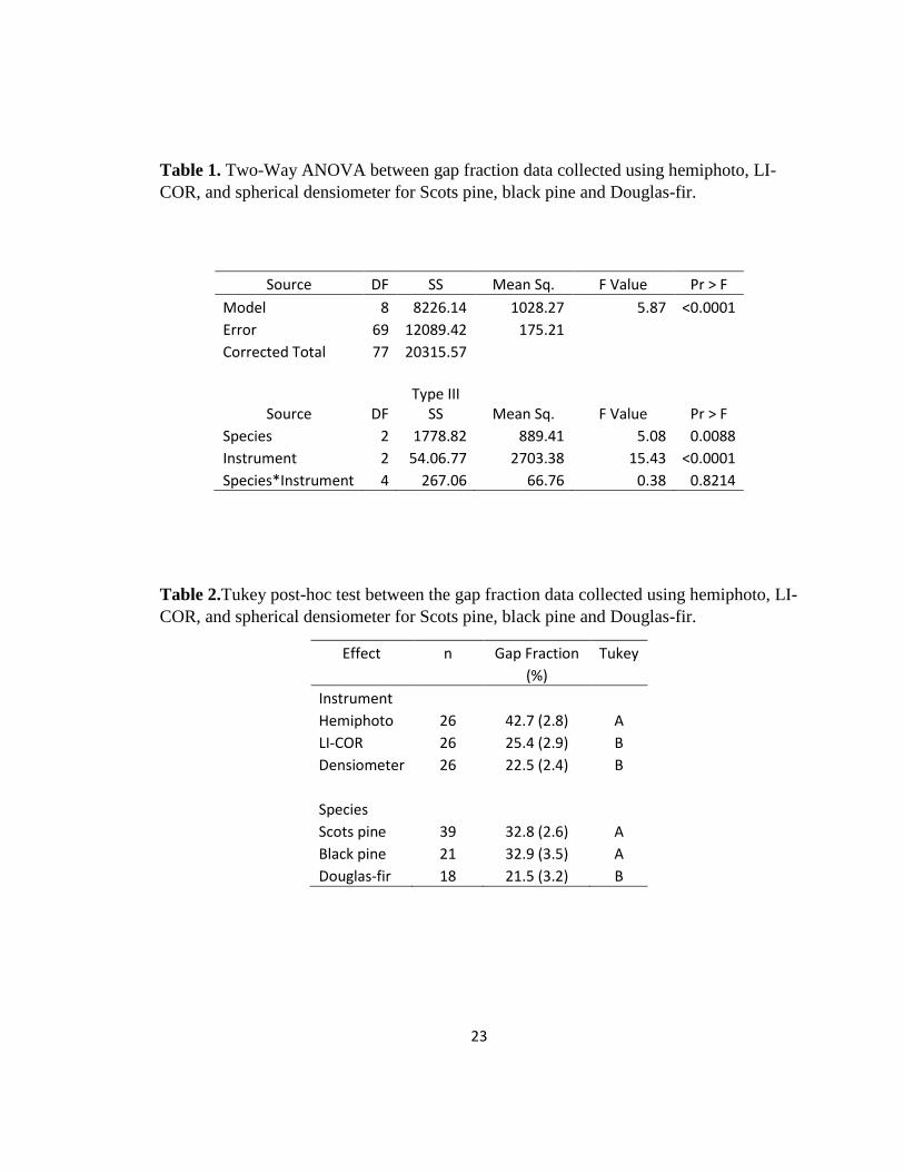
Table 1. Two-Way ANOVA between gap fraction data collected using hemiphoto, LI-COR,
and spherical densiometer for Scots pine, black pine and Douglas-fir. ......................................... 23
Table 2.Tukey post-hoc test between the gap fraction data collected using hemiphoto,
LI-COR, and spherical densiometer for Scots pine, black pine and Douglas-fir. .......................... 23
Table 3. Leaf area index recorded with a LI-COR LAI 2200c Plant Canopy Analyzer
(LI-COR) and hemispherical photography (Hemiphoto) analyzed in Hemiview software
by species. ...................................................................................................................................... 28
Table 4. Single factor ANOVA comparing the leaf area index recorded with a LI-COR
LAI 2200c Plant Canopy Analyzer (LI-COR) and hemispherical photography (Hemiphoto)
between the study sites and species grouping. ............................................................................... 30
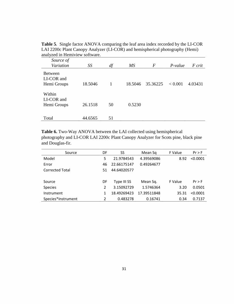
Table 5. Single factor ANOVA comparing the leaf area index recorded by the LI-COR
LAI 2200c Plant Canopy Analyzer (LI-COR) and hemispherical photography (Hemi)
analyzed in Hemiview software. .................................................................................................... 31
Table 6. Two-Way ANOVA between the LAI collected using hemispherical photography
and LI-COR LAI 2200c Plant Canopy Analyzer for Scots pine, black pine and Douglas-fir. ...... 31
Table 7. Single factor ANOVA of canopy density (%) collected by spherical densiometer
and hemispherical photography analyzed in Hemiview software by species. ............................... 33
Table 8. Summary of FuelCalc data used in single factor ANOVA of the canopy bulk
density (CBD) between sites and species. ..................................................................................... 34
Table 9. ANOVA of the Fuelcalc canopy bulk density (CBD) between study sites and the
species. ........................................................................................................................................... 35

vii
Table 10. Summary of data used for single factor ANOVA of the canopy bulk density
(CBD) between Scots Pine, black pine, and Douglas-fir. .............................................................. 35
Table 11. Single factor ANOVA of the canopy bulk density (CBD) between the Scots Pine,
black pine, and Douglas-fir. ........................................................................................................... 35

viii
List of Figures
Page
Figure 1. Satellite image of the Netherlands of the Veluwe (A), the island of Texel (B),
and the southern forested area (C) and plots locations as in white. ............................................... 11
Figure 2. Satellite imagery of the Veluwe located in the Netherlands province of
Gelderland with plots locations in white........................................................................................ 12
Figure 3. Satellite imagery of plot locations in white on the island of Texel. .............................. 13
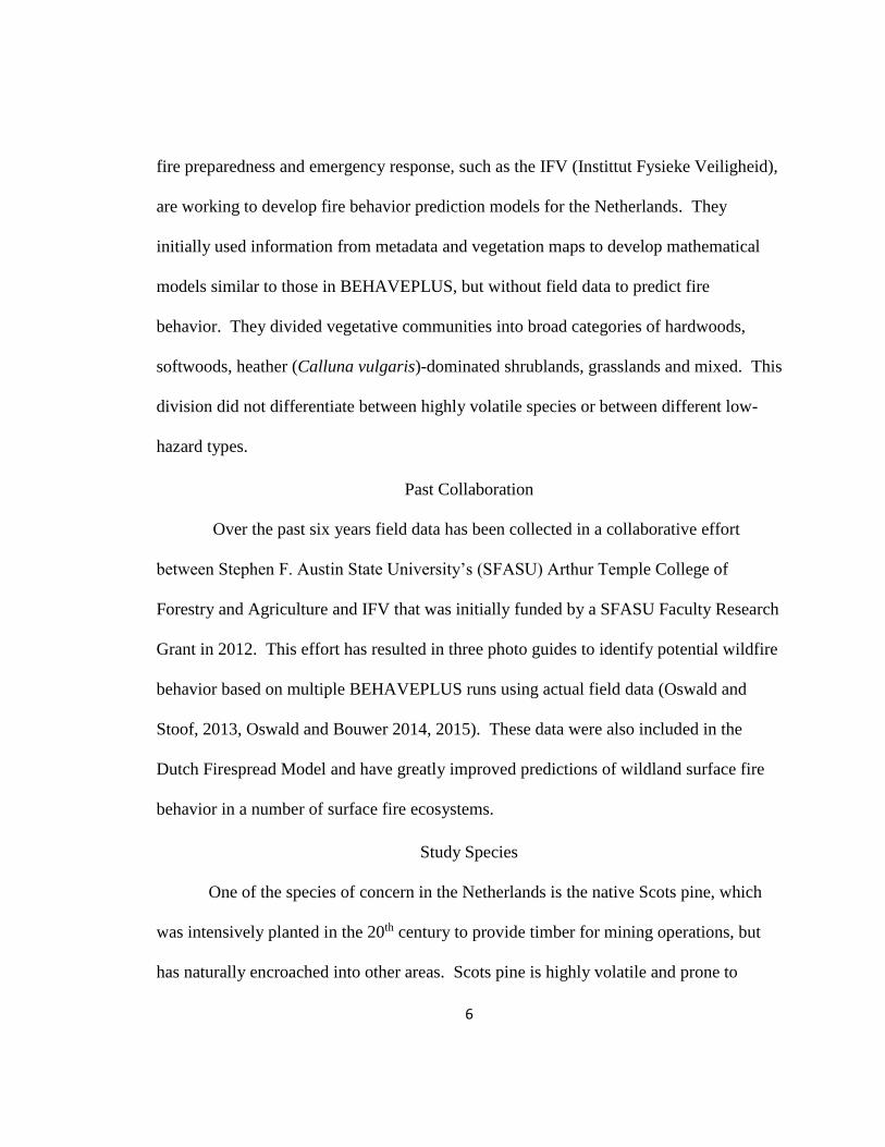
Figure 4. Satellite imagery of the southern Province of Noord-Brabant of the study
area circled and plot locations in white. ........................................................................................ 14
Figure 5. Satellite imagery of plot locations (in white) in the southern forested areas
with the study area circled in white. .............................................................................................. 15
Figure 6. Plot layout schematic plot center S13 marked with a * (from Ottmar, R.D. and
R.E. Vihnanek. 2000.) .................................................................................................................... 16
Figure 7. Scatter gram of gap fraction collected by the densiometer and the hemiphoto
R = 0.795........................................................................................................................................ 24
Figure 8. Scatter gram of gap fraction collected by the LI-COR and the hemiphoto
R = 0.077........................................................................................................................................ 25
Figure 9. Scatter gram of gap fraction collected by the LI-COR and the densiometer
R = 0.017........................................................................................................................................ 26
Figure 10. Scatter gram of LAI collected by the LI-COR and the hemiphoto R = 0.418. ............ 32

ix
List of Appendices
Page
Appendix A. Canopy Bulk Density (CBD) in kg m-3 using FuelCalc 1.4………………...41
Appendix B. Trees per hectare, basal area per hectare, Quadratic Mean Diameter,
total canopy height, and height to live crown by species………………………………..42

1
Introduction
Better understanding of fire behavior can reduce the loss of lives and property.
The Netherlands has a growing wildland urban interface with relatively little fire
expertise. The climate of the Netherlands is changing, experiencing a rising mean
temperature, increasing amount and intensity of precipitation, and the number of drought
periods have increased with more extremely hot days occurring earlier in the year,
increasing the chance of wildland fires. If the Netherlands is to accurately prepare for
wildland fire emergencies, they must continue to build on their understanding of how
wildland fire will behave. Before fire behavior can be estimated, fuel load assessments
must be made in the various vegetative communities across the Netherlands.
Studies conducted in collaboration between Stephen F. Austin State University
and the Instittut Fysieke Veiligheid (IFV), including Oswald and Stoof, (2013), Oswald
and Bouwer (2014, 2015), looked at ground and understory fires, but the area of canopy
fires remain inadequately studied. Forested areas that contain ladder fuels such as vines,
overtopped trees, unpruned lower limbs and downed woody debris can move surface
level fires into the canopy. Canopy fuels can be used in Dutch fire spread models to give
a more accurate and comprehensive representation of the fuels. This study produced data
to be converted into measurements of canopy fuel loads to be used by emergency
preparedness agencies in the Netherlands to anticipate canopy fire behaviors in forested
2
ecosystems. Data were collected on Douglas-fir (Pseudotsuga menziesii (Mirb.) Franco),
Scots pine (Pinus sylvestris L.), and Black pine (Pinus nigra Arn.) in the Netherlands to
estimate canopy bulk density using crown allometry and visual canopy methods, and the
data collected was used in FuelCalc and prepared for use in FARSITE by the Instittut
Fysieke Veiligheid.

3
Goal
The goal of this study was to estimate canopy bulk density of Douglas-fir, black
pine, and Scots pine dominated stands in the Netherlands to be used in fire models
estimating canopy fire behavior in that country. Crown allometry data collected were tree
density (trees per ha), species, condition (live vs. dead), diameter breast height (DBH),
height, and height to live crown base and visual canopy methods using a spherical
densiometer. The specific objectives were:
1: Compare results to determine the optimal method for collection of LAI based on data
quality and efficiency of implementation of methods in the field.
2: Determine if different canopy bulk densities exist for different conditions at sites in the
Netherlands.

4
Literature Review
Background
Wildfires within or adjacent to the Wildland-Urban Interface (WUI) are an
important issue in a number of countries. WUI fires have accounted for nine of the 25
largest fire loss incidents in US history, ranging from $0.5 - $2.4 billion in direct losses
per fire (in 2008 constant dollars, NFPA 2009) and WUI fires continue to cause financial
loss to resources and structures. Utilizing knowledge in fire ecology and fire effects
research over decades by many authors (e. g. Wright and Bailey 1982, Pyne 1996,
Sugihara et al. 2006), fuel loads estimation models (e.g. Brown 1974, Albini 1976,
Anderson 1982, Brown et al. 1982), photo guides for appraising surface fuels ( e.g.
Reeves 1988, Ottmar and Vihnanek 2000), and fire behavior prediction models including
BEHAVE and BEHAVEPLUS (e.g. Deeming et al. 1977, Burgan and Rothermal 1984,
Andrews et al. 2005), fire experts have worked with human-dimension experts to develop
outreach programs. The US Forest Service and the Texas A&M Forest Service have both
adopted this approach for residents in WUIs. Some of the most successful are the
FIREWISE and FIREWISE COMMUNITIES/USA programs (see
www.firewise.org/usa), developed by the National Fire Protection Association (NFPA) in
2001. In 2009, 534 communities and over 531,000 people nation-wide were participating
in FIREWISE activities (NFPA 2009). By 2012, the number exceeded 700 communities.

5
The Netherlands, in an area twice the size of New Jersey and a population of 16.8
million (2013) ranked 30th in the world, has a different WUI issue than the United States
(Centrall Bureau voor Statistiek. 2017). With little wildland fire culture in the public or
political arenas, there is an increasing occurrence of wildland fires, all essentially
occurring within a WUI. The largest contiguous forested area of The Netherlands is the
Veluwe (approximately 1100 km2), located in the central portion of the country (Figures
1 and 2). It includes and is surrounded by small villages, large cities, and a number of
private campgrounds that house up to 3,000-4,000 residents during the peak fire danger
summer months. The area is used extensively for day recreation activities, especially
during dry and warm periods.
In the Netherlands, many fire services often have a strong urban perspective and
do not consider wildfires in their planning or training. During the last 30 years few Dutch
forest organizations have invested in research on wildfire management. While public
perception regarding wildland fire has only recently been evaluated (Brennan 2016),
Dutch awareness of the risk may be low, despite the fact that the areas in which they live
and recreate have considerable fuel loads. Recent incidents in 2009 (Schoorl), 2010
(Bergen, Strabrechtse Heide), and 2014 (De Hoge National Park) have shown the threat
is real, with fires leading to evacuations of about 500 people, and the largest private
collection of Van Gogh paintings in 2014. Fire ecology and management research is
limited in the Netherlands, and instead they currently modify research findings from
other countries using the same or similar species. Dutch agencies involved in wildland
6
fire preparedness and emergency response, such as the IFV (Instittut Fysieke Veiligheid),
are working to develop fire behavior prediction models for the Netherlands. They
initially used information from metadata and vegetation maps to develop mathematical
models similar to those in BEHAVEPLUS, but without field data to predict fire
behavior. They divided vegetative communities into broad categories of hardwoods,
softwoods, heather (Calluna vulgaris)-dominated shrublands, grasslands and mixed. This
division did not differentiate between highly volatile species or between different low-
hazard types.
Past Collaboration
Over the past six years field data has been collected in a collaborative effort
between Stephen F. Austin State University’s (SFASU) Arthur Temple College of
Forestry and Agriculture and IFV that was initially funded by a SFASU Faculty Research
Grant in 2012. This effort has resulted in three photo guides to identify potential wildfire
behavior based on multiple BEHAVEPLUS runs using actual field data (Oswald and
Stoof, 2013, Oswald and Bouwer 2014, 2015). These data were also included in the
Dutch Firespread Model and have greatly improved predictions of wildland surface fire
behavior in a number of surface fire ecosystems.
Study Species
One of the species of concern in the Netherlands is the native Scots pine, which
was intensively planted in the 20th century to provide timber for mining operations, but
has naturally encroached into other areas. Scots pine is highly volatile and prone to

7
canopy fires that may move rapidly, producing extreme fire behaviors and impacts (Hille
2006), and also re-establishes well after fire exposes the mineral soil (Hille and den
Ouden 2004). These forests (Engelmark 1987) become more flammable with fire
exclusion efforts (Komarek, 1983).
Black pine can be found in pure stands, or mixed with Scots pine, and like Scots
pine, does well after a fire as long as the fire clears all other competition, as it is very
shade intolerant (Isajev et al. 2004). Since black pine maybe found alongside Scots pine,
it is thought that they share a similar regeneration history from a periodic stand replacing
fire (Sullivan 1993). Black pine often develop wide flat canopies that, if a fire was able to
gain access to the canopy the fire would likely spread quickly between neighboring trees
(Burns 1990).
Douglas-fir, native to North America, has been established in the Netherlands.
Young trees are considered highly flammable and susceptible to fire due to the thin and
highly resinous bark (Crane, 1982), while mature trees are considered moderately fire
resistant (Revill et al. 1978, Fischer and Bradley 1987, Agee 1993). Fires in such stands
tend to be stand-replacing and exhibit extreme fire behavior (Arno et al. 1995).
Gap Fraction and Canopy Fuels
The gap fraction of a canopy is the fraction of view that is unobstructed by
canopy in any particular direction and is often used in plant physiology studies. Gap
fraction can also be used to calculate and extrapolate canopy fuel data using a correlation
between gap fraction and canopy density if both fuel data and gap fraction are known.

8
Usually, this solar radiation model is based on two attributes: canopy foliage amount and
foliage orientation, and there is an assumption of randomness in the spatial distribution of
the foliage. An indirect method success is determined by how accurately the real canopy
conforms to the modeled data compilation in the radiation model, with models fueled by
larger volumes of measurements having a higher average accuracy. Gap fraction can be
estimated by several different methods, including the use of a spherical densiometer, Li-
COR plant canopy analyzer, and by hemispherical photograph interpretation. When
measuring the gap fraction using LI-COR systems, five angles of view are computed by
dividing the below-canopy readings by the above-canopy readings from the stand. The
LI-COR’s light sensor includes a filter to limit the spectrum of received radiation to <490
nm, minimizing the effect of light scattered by foliage (Welles and Cohen 1996). While
using the LI-COR the sunlight should be obscured since the directly illuminated foliage
will scatter more light in the canopy than will be calculated by the equipment after the
above canopy reference reading, reducing LAI values up to 50% (Welles and Norman,
1991). Gap fractions are computed from hemispherical photography by determining the
fraction of exposed background within rings or bands about the center of the photograph
using a softer ware such as Hemiview canopy analysis software (Anderson, 1964). In one
study, Keene et al. (2005) found during their measurements of gap fraction to calculate
CBD, that increasing the number of sample grid points above one point did not improve
the estimate while using the LAI2000 and hemiphoto techniques.

9
Units of Measurement for Canopy Fuels
Four parameters are required to determine canopy fuel loads: canopy base height,
canopy height, canopy cover, and canopy bulk density. Bulk density (the mass of the fuel
divided by the total volume) is an important parameter in estimating canopy fire
behavior. “Canopy bulk density is the amount of burnable canopy fuel by canopy volume
(kg m-3) and represents the degree of packing of canopy fuels” (Keene 2015). Canopy
bulk density is used to estimate crown fire propagation in fire spread models such as
FARSITE (Finney 1998), while surface fuel bulk densities are used to estimate surface
fire intensities (Keane 2015). The challenges in estimating canopy bulk densities are
many, and are often tied to the determination of what is the real volume occupied by a
tree. As a result, various direct and indirect methods have been developed to obtain this
important parameter. Direct methods including the destructive sampling of trees and
intensive analysis of needle count, weight, and area. Destructive sampling (cutting entire
trees and measuring all canopy fractions for each tree) is extremely time consuming and
problematic (Keane 2015). Indirect methods include the use of a LI-COR LAI 2200c
Plant Canopy Analyzer, hemispherical photography, and spherical densiometer (Keane
2015).

10
Methods
Site Locations
This study was conducted within the Netherland’s primary forested area of the
Veluwe (Figures 1 and 2), the forested coast on the island of Texel (Figures 3 and 4), and
a recently burned forested area in the south of the Netherlands (Figures 5 and 6). All
black pine plots were located on the island of Texel, and no other species plots were
measured on the island. Douglas-fir plots were all located within the Veluwe. Scots Pine
was sampled in two areas. The first was located within the southern half of the Veluwe
and contained a visually denser understory, with Scots Pine dominating the canopy with a
mixture of hardwoods. The second was located 111 kilometers to the southwest of the
Veluwe. The site had experienced a fire within the last three years and had a clear
understory with almost no midstory (IFV staff personal communication). The southern
Scots pine was reported by IFV to be on average older that the central Scots pine with the
area being a mixture of open parklike older pines and two plots within developing
plantations. Many of the other plot locations were used in previous studies to compile
understory fuel data used in modeling surface fires (Oswald and Stoof 2013, Oswald and
Brouwer 2014, 2015).

11
Figure 1. Satellite image of the Netherlands of the Veluwe (A), the island of Texel (B),
and the southern forested area (C) and plots locations as in white.
B
A
C

12
Figure 2. Satellite imagery of the Veluwe located in the Netherlands province of
Gelderland with plots locations in white.

13
Figure 3. Satellite imagery of plot locations in white on the island of Texel.
14
Figure 4. Satellite imagery of the southern Province of Noord-Brabant of the study area circled and plot locations in white.

15
Figure 5. Satellite imagery of plot locations in white in the southern forested area.

16
Field Layout
Within each of the sites selected by IFV, a 400 m² plot (11.2 m radius) was
established at point S13 in the center of previously utilized plots (Oswald and Stoof 2013,
Oswald and Brouwer 2014, 2015) (Figure 6.) All trees greater than 2 m in height were
measured for dbh (diameter to breast height) (cm) using a diameter tape, and both total
height (m) and height to live crown (m), measured with a clinometer. In addition, a
spherical densiometer was used to measure canopy cover, with four measurements taken
in the cardinal directions and a mean canopy cover determined. Hemispherical
photographs were also taken at that same point.
Figure 6. Plot layout schematic plot center S13 marked with a * (from Ottmar, R.D. and R.E.
Vihnanek. 2000.)

17
Field Sampling
Since destructive sampling (cutting entire trees and measuring all canopy
fractions for each tree) is extremely time-consuming and problematic (Keane 2015), and
government approval could not be obtained, indirect methods were used to obtain the
various canopy fuel variables.
LI-COR LAI 2200c Plant Canopy Analyzer
A LI-COR LAI 2200c Plant Canopy Analyzer (hereafter LI-COR) was used to
measure leaf area index (hereafter LAI). LAI is a unitless measurement of single-sided
leaf area per unit ground surface area, is a relatively accurate measure of canopy foliage,
and is the most important fuel parameter for determining canopy bulk density. The LI-
COR estimates gap fraction as the fraction of radiation transmitted through the canopy at
five zenith angles (7°, 23°, 38°, 53°, and 68° from vertical) measured with five concentric
lenses on a handheld wand (Welles and Norman 1991). The wand was modified with a
45° lens because of the size of the plot, and to reduce the chance to include the operator’s
body in the readings. An initial measurement was taken in an adjacent area with no
canopy cover to obtain a base light level reading and then thirty measurements were
taken at random locations inside the plot, followed by a final measurement in the adjacent
area in case the base light level changed during the stand measurements. A consistent
state of light conditions is required to properly compare sites, and is normally done in the
early morning or at dusk: due to the Netherlands’ usual weather conditions with overcast
skies, it was easy to have consistent measurement conditions. On days with prolonged

18
periods of cloud cover, the LI-COR measurements were the focus of that day and other
measurements were delayed to increase the number of sites measured in similar lighting
conditions.
Hemispherical Canopy Photography
Camarillo et al. (2015) is one of the recent studies that used a hemispherical
canopy photography (hereafter hemiphoto) technique to measure LAI (Rich, 1990; Evans
and Coombe, 1959). Using fish-eye lens under the canopy, it is possible to obtain a
permanent measure of canopy structure (Rich, 1990; Hale and Edwards, 2002) within a
180-degree projection from plot center. Photos are then interpreted by splitting pixels into
sky or canopy, and then converted into indices using an inversion model based on Beer’s
Law, using the observed gap fraction distribution throughout the photo (Rich, 1990; Rich
et al., 1993). For this study a SIGMA SD15 digital camera with a 4.5 mm 1:2.8 fisheye
lens (SIGMA Japan) was set 1.3 m above the ground on a tripod, levelled, and
photographs taken on days with overcast skies to reduce errors by minimizing reflected
light from leaves and boles and increasing contrast between sky and canopy. Photographs
were analyzed using SideLook version 1.1 to determine thresholds for pixel classification
(Nobis and Hunziker 2005). Once thresholds were established, Hemiview canopy
analysis software (Delta-T Devices, England) was used to calculate LAI for each photo.
19
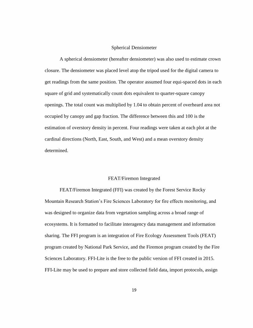
Spherical Densiometer
A spherical densiometer (hereafter densiometer) was also used to estimate crown
closure. The densiometer was placed level atop the tripod used for the digital camera to
get readings from the same position. The operator assumed four equi-spaced dots in each
square of grid and systematically count dots equivalent to quarter-square canopy
openings. The total count was multiplied by 1.04 to obtain percent of overheard area not
occupied by canopy and gap fraction. The difference between this and 100 is the
estimation of overstory density in percent. Four readings were taken at each plot at the
cardinal directions (North, East, South, and West) and a mean overstory density
determined.
FEAT/Firemon Integrated
FEAT/Firemon Integrated (FFI) was created by the Forest Service Rocky
Mountain Research Station’s Fire Sciences Laboratory for fire effects monitoring, and
was designed to organize data from vegetation sampling across a broad range of
ecosystems. It is formatted to facilitate interagency data management and information
sharing. The FFI program is an integration of Fire Ecology Assessment Tools (FEAT)
program created by National Park Service, and the Firemon program created by the Fire
Sciences Laboratory. FFI-Lite is the free to the public version of FFI created in 2015.
FFI-Lite may be used to prepare and store collected field data, import protocols, assign
20
plots and monitoring areas, and to export data in to formats needed for use in other
monitoring software. The main differences in the government and public software is FFI-
Lite does not support password security, user roles, data entry by personal digital
assistants, or use of the geographic information system (GIS) toolbar.
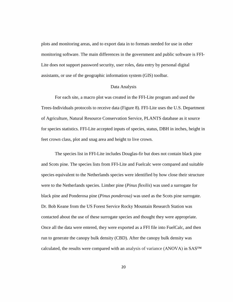
Data Analysis
For each site, a macro plot was created in the FFI-Lite program and used the
Trees-Individuals protocols to receive data (Figure 8). FFI-Lite uses the U.S. Department
of Agriculture, Natural Resource Conservation Service, PLANTS database as it source
for species statistics. FFI-Lite accepted inputs of species, status, DBH in inches, height in
feet crown class, plot and snag area and height to live crown.
The species list in FFI-Lite includes Douglas-fir but does not contain black pine
and Scots pine. The species lists from FFI-Lite and Fuelcalc were compared and suitable
species equivalent to the Netherlands species were identified by how close their structure
were to the Netherlands species. Limber pine (Pinus flexilis) was used a surrogate for
black pine and Ponderosa pine (Pinus ponderosa) was used as the Scots pine surrogate.
Dr. Bob Keane from the US Forest Service Rocky Mountain Research Station was
contacted about the use of these surrogate species and thought they were appropriate.
Once all the data were entered, they were exported as a FFI file into FuelCalc, and then
run to generate the canopy bulk density (CBD). After the canopy bulk density was
calculated, the results were compared with an analysis of variance (ANOVA) in SAS™

21
software (SAS Institute Inc. 2011) using a significance factor of 0.05, to determine if
there was a difference within or between sites based on both species and species site
grouping.
The gap fractions were compared using the GLM procedure to run a Two-Way
ANOVA between the gap fraction values, instruments, and species. The GLM procedure
was selected due to the uneven number of plots between the three species. This analysis
also produced multiple scatter grams. To determine the source of any variation a Tukey
test was run to identify which variables were significantly different. The LAI data
recordings were also run through SAS using GLM between the variation between the
LAI values, instruments, and species. A post-hoc Tukey test was conducted to determine
a difference between the variables that showed a significant difference from other
variables.

22
Results and Discussion
Gap Fraction Comparisons
A GLM procedure was used to run a Two-Way ANOVA between the gap fraction
values, instruments, and species (Table 1), and a Tukey test was then performed to
identify means that were significantly different from each other (Table 2). Scots pine and
black pine were similar in gap fraction, but were significantly different than Douglas-fir.
Between methods of data collection, data collected by the LI-COR and densiometer were
similar but were significantly different than that of the hemiphoto. Scatter grams were
created to show the relationship between gap fraction data collected by the densiometer
and the hemiphoto, LI-COR and the hemiphoto, and the LI-COR and densiometer
(Figures 7, 8, and 9).
23
Table 1. Two-Way ANOVA between gap fraction data collected using hemiphoto, LI-
COR, and spherical densiometer for Scots pine, black pine and Douglas-fir.
Source DF SS Mean Sq. F Value Pr > F
Model 8 8226.14 1028.27 5.87 <0.0001
Error 69 12089.42 175.21
Corrected Total 77 20315.57
Source DF Type III
SS Mean Sq. F Value Pr > F
Species 2 1778.82 889.41 5.08 0.0088
Instrument 2 54.06.77 2703.38 15.43 <0.0001
Species*Instrument 4 267.06 66.76 0.38 0.8214
Table 2.Tukey post-hoc test between the gap fraction data collected using hemiphoto, LI-
COR, and spherical densiometer for Scots pine, black pine and Douglas-fir.
Effect n Gap Fraction Tukey
(%) Instrument Hemiphoto 26 42.7 (2.8) A
LI-COR 26 25.4 (2.9) B
Densiometer 26 22.5 (2.4) B
Species Scots pine 39 32.8 (2.6) A
Black pine 21 32.9 (3.5) A
Douglas-fir 18 21.5 (3.2) B

24
Figure 7. Scatter gram of gap fraction collected by the densiometer and the hemiphoto R
= 0.795.
.
5.
10.
15.
20.
25.
30.
35.
40.
45.
50.
. 10. 20. 30. 40. 50. 60. 70.
De
nsi
om
eter
Gap
Fra
ctio
n (
%)
Hemiphoto Gap Fraction (%)

25
Figure 8. Scatter gram of gap fraction collected by the LI-COR and the hemiphoto R =
0.077.
.
10.
20.
30.
40.
50.
60.
70.
. 10. 20. 30. 40. 50. 60. 70.
LI-C
OR
Gap
Fra
ctio
n (
%)
Hemiphoto Gap Fraction (%)

26
Figure 9. Scatter gram of gap fraction collected by the LI-COR and the densiometer R =
0.017.
Leaf Area Index Comparisons
A comparison between the LAI readings from the LI-COR and the hemiphoto
revealed variations between the two methods (Table 3). No significant difference
between the species were found between the LAI from the LI-COR and the hemiphoto
using a single factor ANOVA at α 0.05 (Table 4). A two-way ANOVA was then
performed to determine if there was a significant difference between the LAI recorded by
.
10.
20.
30.
40.
50.
60.
70.
. 10. 20. 30. 40. 50.
LI-C
OR
Gap
Fra
ctio
n (
%)
Densiometer Gap Fraction (%)

27
the LI-COR and hemispherical photography, and a significant difference was found
(Table 5). On average, the LI-COR were two to three times larger than the recordings
calculated from the hemiphoto. The only site that had a greater LAI recorded by the
hemiphoto was a Scots pine plot in the southern forested area. A possible explanation to
this was the plot density of 2150 trees per ha. The plot also had a large number of dead
trees on the site, either standing or those leaning against other live trees. While the
hemiphoto was conducted from the center of the plot, the LI-COR was moved
continuously between readings. The open areas provided by the dead trees many have
caused a bias if the user of the LI-COR unconsciously moved between open spots with
easier access due to the absence of live trees; conversely, this may not have been a factor
since the gap may have been filled by adjacent live trees.
The highest LAI was found in the Douglas-fir sites, which had a regeneration
cohort not observed at the other sites, mostly young Douglas-fir, creating areas with high
densities alongside areas mostly clear under and around the larger canopies of the mature
trees. A Two-Way ANOVA GLM procedure was run between the LAI values,
instruments, and species (Table 6), and a Tukey test was run to identify means that were
significantly different. There was no significant difference between species, but there was
a significant difference between the LI-COR and hemiphoto. A scatter gram was created
to show the relationship between the LI-COR and the hemiphoto (Figure 10).

28
Table 3. Leaf area index recorded with a LI-COR LAI 2200c Plant Canopy Analyzer
(LI-COR) and hemispherical photography (Hemiphoto) analyzed in Hemiview software
by species.
Species Site LI-COR Hemiphoto
Densiometer
Canopy
Density
Hemiphoto
Canopy
Density (LAI) (LAI) (%) (%)
Black Pine BP 1 0.99 0.47 63.9 40.9
BP 2 1.91 0.40 71.1 41.9
BP 3 1.17 0.57 73.2 45.3
BP 4 2.37 0.79 71.7 58.2
BP 5 1.64 0.62 84.4 51.5
BP 6 2.65 1.09 85.7 68.6
BP 7 1.34 0.77 87.8 58.2
Douglas-fir DF 1 3.43 0.48 54.2 45.4
DF 2 1.76 1.07 84.4 69.4
DF 3 3.37 1.14 74.5 70.0
DF 4 2.30 1.34 94.3 74.8
DF 5 2.32 1.53 96.6 78.0
DF 6 2.41 1.16 85.7 70.3
Scots Pine SP 1 1.73 0.76 71.7 57.7
SP 2 1.13 0.51 54.5 47.1
SP 3 1.29 0.51 72.4 47.6
SP 4 1.13 0.44 72.4 43.8
SP 5 2.01 0.77 93.5 59.4
SP 6 4.18 1.52 95.6 78.3
F 1 1.68 0.54 81.3 45.1
F 2 1.44 0.55 73.2 49.2
F 3 1.50 0.52 60.7 46.2
F 4 1.11 0.52 69.1 41.8
F 5 3.81 1.31 67.0 71.3
F 6 0.56 1.56 82.3 75.0
F 7 3.29 0.57 93.5 49.5

29
The LAI values from the hemiphoto and LI-COR were compared to those of other
studies. Black pine LAI recorded in Spain were more similar to the hemiphoto than the
LI-COR (Navarro-Cerrillo et al. 2016), but Scots pine LAI gathered in Belgium was
more similar to the LAI from the LI-COR (Xiao et al. 2006) sites. The LAI of Douglas-fir
estimated in Washington State was more similar to the LAI recorded by the hemiphoto
than the LI-COR, although that study was in an old growth stand (Thomas and Winner
2000). There was a large range in the LAI in the Washington study, ranging from 1.1 to
8.6 depending on the stand density at each site.

30
Table 4. Single factor ANOVA comparing the leaf area index recorded with a LI-COR
LAI 2200c Plant Canopy Analyzer (LI-COR) and hemispherical photography
(Hemiphoto) between the study sites and species grouping.
Source of
Variation SS df MS F P-value F crit
LI-COR
Between
Species
Groups 2.7697 3 0.9232 1.030157 0.398523 3.049125
Within
Species
Groups 19.7166 22 0.8962
Total 22.4864 25
Hemiphoto
Between
Species
Groups 0.7223 3 0.2407 1.802427 0.176191 3.049125
Within
Species
Groups 2.9387 22 0.1335
Total 3.6611 25
31
Table 5. Single factor ANOVA comparing the leaf area index recorded by the LI-COR
LAI 2200c Plant Canopy Analyzer (LI-COR) and hemispherical photography (Hemi)
analyzed in Hemiview software.
Source of
Variation SS df MS F P-value F crit
Between
LI-COR and
Hemi Groups 18.5046 1 18.5046 35.36225 < 0.001 4.03431
Within
LI-COR and
Hemi Groups 26.1518 50 0.5230
Total 44.6565 51
Table 6. Two-Way ANOVA between the LAI collected using hemispherical
photography and LI-COR LAI 2200c Plant Canopy Analyzer for Scots pine, black pine
and Douglas-fir.
Source DF SS Mean Sq F Value Pr > F
Model 5 21.9784543 4.39569086 8.92 <0.0001
Error 46 22.66175147 0.49264677
Corrected Total 51 44.64020577
Source DF Type III SS Mean Sq. F Value Pr > F
Species 2 3.15092729 1.5746364 3.20 0.0501
Instrument 1 18.49269423 17.39511848 35.31 <0.0001
Species*Instrument 2 0.483278 0.16741 0.34 0.7137

32
Figure 10. Scatter gram of LAI collected by the LI-COR and the hemiphoto R = 0.418.
The canopy densities calculated from the densiometer and the hemiphoto
analyzed in Hemiview software were compared (Table 4), and a significant difference
between the canopy densities recorded by the densiometer and hemiphoto was found. The
difference is potentially from two main factors. First, the canopy area the densiometer
used to calculate canopy density is less than the area utilized by the hemiphoto. While
both take their data from a circle, the area used to calculate canopy density on the
spherical densiometer comes from a grid 49% of the total surface area on the mirror, and
not the full area of the mirror. This allows the user to make estimations of cover area
quickly but does result in a smaller overall canopy section being analyzed and potential
0
0.2
0.4
0.6
0.8
1
1.2
1.4
1.6
1.8
0 0 . 5 1 1 . 5 2 2 . 5 3 3 . 5 4 4 . 5
HEM
IPH
OTO
LA
I
LI-COR LAI

33
errors have been noted (Vales, et al. 1988; Englund, et al. 2000) While using hemiphoto,
the Hemiview software utilizes the entire area of the photograph taken in its calculations,
as well as determining by pixel if the area is sky or what the software determines as
canopy.
A second reason is the approach the two methods used to calculate canopy
density. Using the spherical densiometer, the canopy density is calculated by the user’s
ocular estimation of the percent of open canopy within squares on the densiometer. When
this method is compared to the pixel by pixel analyze done by the Hemiview software,
the human bias becomes a defining difference between the analysis methods. While the
ease of use provided by the densiometer is much greater than the hemiphoto due to the
simpler field methods and lower cost of materials, the added sample size and level of
detail provided by the hemiphoto makes it a better choice for canopy density.
Table 7. Single factor ANOVA of canopy density (%) collected by spherical densiometer
and hemispherical photography analyzed in Hemiview software by species.
Source of
Variation SS df MS F P-value F crit
Between
Densiometer
and Hemi
Groups 5408.004 1 5408.004 34.13211 < 0.001 4.03431
Within
Groups 7922.164 50 158.4433
Total 13330.17 51

34
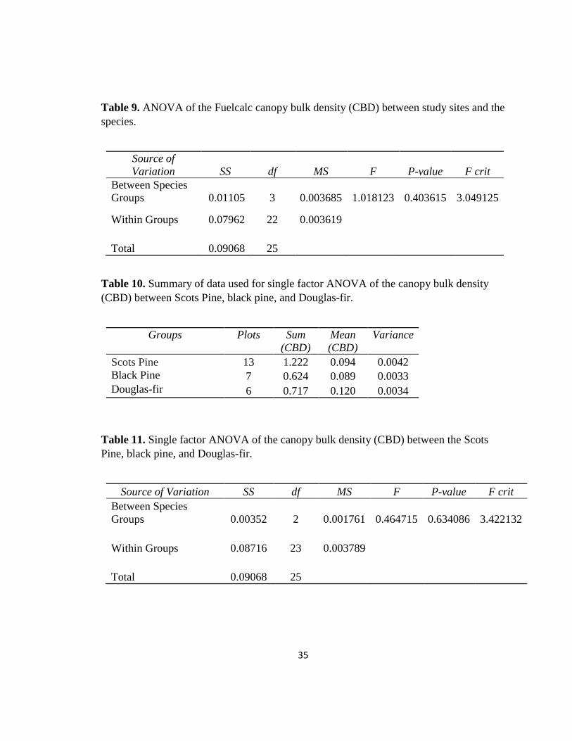
Canopy Bulk Density
No significant difference was found for canopy bulk density between sites or
species (Tables 8, 9, 10 and 11). One factor that may explain the similarity between
species would be the method Fuelcalc uses to determine canopy bulk density. Fuelcalc
does not use data from hardwoods when determining canopy bulk density because the
focus of the software is on the dominated species in the canopy, so any hardwoods under
the dominant pine canopy would not be captured. The results of the single factor
ANOVA found the dominant Douglas-fir had the highest average canopy bulk density
(Table 12); a possible explanation of this could be the larger canopies of the mature
Douglas-fir compared to Scots Pine and Black Pine (Burns 1990, Hummel 2009).
Table 8. Summary of FuelCalc data used in single factor ANOVA of the canopy bulk
density (CBD) between sites and species.
Groups
Plots
Sum
(CBD)
Mean
(CBD)
Variance
Black Pine 7 0.624 0.08914 0.00325 Douglas Fir 6 0.717 0.11950 0.00344 Southern Scots
Pine 7 0.814 0.11629 0.00647 Scots Pine 6 0.408 0.06800 0.00082
35
Table 9. ANOVA of the Fuelcalc canopy bulk density (CBD) between study sites and the
species.
Source of
Variation SS df MS F P-value F crit
Between Species
Groups 0.01105 3 0.003685 1.018123 0.403615 3.049125
Within Groups 0.07962 22 0.003619
Total 0.09068 25
Table 10. Summary of data used for single factor ANOVA of the canopy bulk density
(CBD) between Scots Pine, black pine, and Douglas-fir.
Groups
Plots
Sum
(CBD)
Mean
(CBD)
Variance
Scots Pine 13 1.222 0.094 0.0042 Black Pine 7 0.624 0.089 0.0033 Douglas-fir 6 0.717 0.120 0.0034
Table 11. Single factor ANOVA of the canopy bulk density (CBD) between the Scots
Pine, black pine, and Douglas-fir.
Source of Variation SS df MS F P-value F crit
Between Species
Groups 0.00352 2 0.001761 0.464715 0.634086 3.422132
Within Groups 0.08716 23 0.003789
Total 0.09068 25

36
Conclusions
Gap Fraction The difference in the canopy gap fractions of Scots pine and black pine compared
to Douglas-fir was different than the results seen in the LAI and canopy bulk density
analysis. The LI-COR and densiometer were similar, but were significantly different than
the data collected by the hemiphoto, similar to the comparison between the hemiphoto
and the LI-COR when comparing LAI. The pines similar gap fractions fits the trends
between pine species, but Douglas-Fir was expected to also have a similar trend like the
pines based on the LAI and canopy bulk density data.
Leaf Area Index
The analysis of leaf area index found no significant difference between species,
but there was a significant difference between the leaf area indexes calculated by LI-COR
and hemiphoto. This was in contrast with the analysis of gap fraction showing significant
difference between the species. The difference between the leaf area index based on
species sampled was p = 0.0501 and a larger sample size might determine if this is a
biological or sampling result.
37
Canopy Bulk Density
With no significant difference in the mean CBD between the species or species
groups, it appears a canopy fire would act similarly for each of the species if based on
CBD alone. While the CBD of the plots may have been similar, the site conditions were
not and the variation would also be a factor of how a fire would act. During the
calculations of CBD, Fuelcalc is designed to exclude hardwoods from its calculation as
default action based on the premise that hardwoods do not contribute significantly to
crown fire activity. As the majority of the plots were dominated by their respective
species of black pine, Douglas-fir, and Scots pine with only a few canopy level
hardwoods, this would apply here; however, in some plots on Texel the hardwoods
located in the midstory did have a potential to act as ladder fuels into those canopies.
Douglas-fir’s mean CBD was higher than the other species, and may have been caused by
the larger canopies on the mature Douglas-fir compared to Scots pine and black pine,
and/or the large amounts of regeneration found at the Douglas-fir plots.

38
Management Implementations and Recommendations
Gap Fraction
By obtaining a larger sample size confirming the relationship between gap
fraction of the three species compared to the relationship not seen in canopy bulk density
and leaf area index, an accurate correlation could be drawn between gap fraction and
canopy bulk density for similar sites, as well as one for leaf area index. This could be
used for quick data recording to gather data from the species in sites in similar areas to
add more information to the fire spread models.
Leaf Area Index
The hemiphoto is recommended for use during any future data collection. While
the LI-COR was easier to transport and gave the fastest recorded measurement of LAI, its
infield collection speed was slower than the hemiphoto. The method of data collection
was tied to the lack of consistency of the overcast sky as there were at times rapid
changes between overcast and rain. As both pieces of equipment use lens to obtain light
readings, this caused issues by the occasional wetting of the lens requiring additionally
time for lens maintenance. Since the hemiphoto only needed a single photograph to
determine LAI versus the 32 reading required by the LI-COR, if the light consistency
changed or precipitation began during a plot sampling, then the hemiphoto would have
the greatest chance to collect data in adverse circumstances. The downside to the

39
hemiphoto is the extra step of analysis between field measurement and receiving LAI
results. While it is an time consuming method and possibly more so in the Netherlands
due to environmental and social regulations, destructive sampling in the study plots
would allow for a comparison of the direct and indirect methods and allow for an analyze
of precision of the measured LAI by both the LI-COR and hemiphoto. Future analysis
using destructive sampling and analysis is highly recommended to confirm the results of
this study.
Canopy Density
For determining canopy density, the hemiphoto is also recommended for field
use. Unless an immediate number is needed, the increased precision found in the digital
analyzed photos appears the best method. By using the photographic analysis some
human error is reduced. The use of a mean dot count using the spherical densiometer is
designed to reduce the error by each user. The operator error using the hemiphoto is still
present when acquiring data, so a standard protocol for photography would also help
standardize results. The main benefits appears to be the pixel level digital analyses the
photography delivers when put through SideLook and Hemiview, which are believed to
be a better representation that the spherical densitometers estimation. If hemiphoto
becomes the method of LAI collection, then the data needed to calculate canopy density
and gap fraction will also be collected in the same photograph. The downside of the use
of hemiphoto is the initial cost of equipment and software and the increase in time

40
between field data collection and results since the photographs need to be analyzed
before canopy densities can be determined.
Future Research
This study indicates there is a difference between the canopy fuel load
measurements results between the methods of measurement but not between species or
sites. A continuation of this research should be conducted to expand and verify results to
increase the scope of the estimation ability of the Dutch fire behavior models, and a
larger sample size is recommended to determine if there is a difference in canopy fuel
loads between species or are there differentiating site factors. Continued research over a
larger area should be pursued to increase the applicability of the Dutch fire spread
models. Destructive sampling would allow for a comparison of the direct and indirect
methods and allow for analyze of the accuracy and precision of the measured leaf area
index, canopy density, and canopy bulk density.
One advantage the United States has in fire ecology is the ability to draw on a
long history of wildland fires and an extended knowledge base developed of decades of
fire effects research on vegetation, water, air and wildlife through numerous studies as
well as generations of authors. This research allowed for the development and
implementation and improvement in fuel loads estimation models, for fire behavior
prediction models such as FARSITE and BEHAVEPLUS, each building off of past
research while contributing more to the collective knowledge of fire ecology in the
country.
41
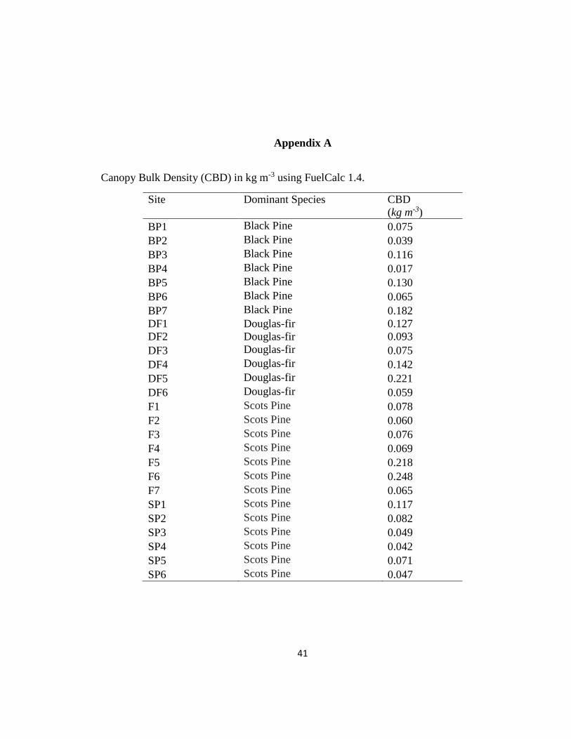
Appendix A
Canopy Bulk Density (CBD) in kg m-3 using FuelCalc 1.4.
Site
Dominant Species
CBD
(kg m-3)
BP1 Black Pine 0.075
BP2 Black Pine 0.039
BP3 Black Pine 0.116
BP4 Black Pine 0.017
BP5 Black Pine 0.130
BP6 Black Pine 0.065
BP7 Black Pine 0.182
DF1 Douglas-fir 0.127
DF2 Douglas-fir 0.093
DF3 Douglas-fir 0.075
DF4 Douglas-fir 0.142
DF5 Douglas-fir 0.221
DF6 Douglas-fir 0.059
F1 Scots Pine 0.078
F2 Scots Pine 0.060
F3 Scots Pine 0.076
F4 Scots Pine 0.069
F5 Scots Pine 0.218
F6 Scots Pine 0.248
F7 Scots Pine 0.065
SP1 Scots Pine 0.117
SP2 Scots Pine 0.082
SP3 Scots Pine 0.049
SP4 Scots Pine 0.042
SP5 Scots Pine 0.071
SP6 Scots Pine 0.047

42
Appendix B
Trees per hectare, basal area per hectare, Quadratic Mean Diameter, total canopy height,
and height to live crown by species.
Species Site TPHA BA QMD TH HLC (m2/ha) (cm) (m) (m)
Black Pine BP 1 300 13.23 23.70 9.35 6.63
BP 2 450 9.16 16.10 6.76 1.90
BP 3 400 18.55 24.30 11.6 7.40
BP 4 575 5.50 11.04 6.10 1.74
BP 5 875 31.91 21.55 12.99 8.28
BP 6 1475 13.51 10.80 7.58 4.34
BP 7 700 36.88 25.93 13.40 9.17
Douglas-fir DF 1 1925 20.98 11.78 16.97 0.10
DF 2 1425 11.15 9.98 8.05 2.70
DF 3 350 14.25 22.77 18.81 9.80
DF 4 425 36.09 32.88 26.45 17.35
DF 5 500 46.44 34.49 28.5 17.4
DF 6 300 11.86 22.44 16.64 6.93
Scots Pine SP 1 575 19.02 20.52 10.75 7.04
SP 2 500 16.60 20.56 16.73 10.72
SP 3 325 12.08 21.75 16.37 9.17
SP 4 300 15.19 25.39 16.51 8.36
SP 5 625 14.20 17.01 17.30 10.90
SP 6 1050 21.54 16.16 18.21 9.53
F 1 275 19.22 29.83 17.32 10.81
F 2 250 11.71 24.43 13.29 6.74
F 3 250 17.94 30.23 20.06 13.69
F 4 150 16.48 37.40 19.71 12.55
F 5 2500 38.16 13.94 18.19 14.33
F 6 2150 36.09 14.62 17.33 15.31
F 7 350 20.53 27.33 20.90 13.48
43
Literature Cited
Abrams, M. D. (1992). Fire and the development of oak forests. BioScience, 42(5), 346-
353.
Agee, J. K. (1993). Alternatives for implementing fire policy. In Proceedings,
Symposium on fire in wilderness and park management (pp. 107-112).
Albini, F. (1976). Estimating wildfire behavior and effects. USDA Forest Service,
Intermountain Forest and Range Experiment Station, General Technical Report INT-30,
92 pp.
Anderson, H. E. (1982). Aids to determining fuel models for estimating fire behavior.
Ogden: U.S.D.A.
Anderson MC. 1964. Studies of the woodland light climate. 1. The photographic
computation of light conditions. Journal of Ecology 52, 27-41.
Arno, S. F., Scott, J. H., & Hartwell, M. G. (1995). Age-class structure of old growth
ponderosa pine/Douglas-fir stands and its relationship to fire history (p. 25). US
Department of Agriculture, Forest Service, Intermountain Research Station.
Brennan, A. (2016). Determining Public Perceptions toward Wildland Fire in the
Veluwe Region of the Netherlands. 58 pp.
Brown, J. K. (1974). Handbook for inventorying downed woody material. Ogden, UT:
Intermountain Forest and Range Experiment Station, Forest Service, U.S. Dept. of
Agriculture.
Brown, J. K., Oberheu, R. D., & Johnston, C. M. (1982). Handbook for inventorying
surface fuels and biomass in the Interior West. Ogden, UT: USFS.
Burgan, R. and Rothermel, R. (1984). BEHAVE : fire behavior prediction and fuel
modeling system -- FUEL subsystem. USDA Forest Service, Intermountain Forest and
Range Experiment Station, 126 pp.
Burns, R. and Honkala B. (1990).Silvics of North America: 1. Conifers. Agriculture
Handbook654. U.S. Department of Agriculture, Forest Service, Washington, DC. vol. 1,
675 pp.
44
Camarillo, S. A., Stovall, J. P., & Sunda, C. J. (2015). The impact of Chinese tallow
(Triadica sebifera) on stand dynamics in bottomland hardwood forests. Forest Ecology
and Management, 344, 10-19.
Centrall Bureau voor Statistiek. (2017). Population; key figures November 01 2017.
Retrieved from https://www.cbs.nl/en-gb
Crane, M. F. (1982). Fire ecology of Rocky Mountain Region forest habitat types. Final
Report Contract No. 43-83X9-1-884. Missoula, MT: USDA Forest Service, Region 1.
272 p. On file with: USDA Forest Service, Intermountain Research Station, Fire Sciences
Laboratory, Missoula, MT.
Deeming, J.E., Burgan, R.E., and Cohen, J.D. (1977). The national fire-danger rating
system - 1978. USDA For. Ser. Gen. Tech. Rep. INT-39.
Engelmark, O. (1987). Fire history correlations to forest type and topography in northern
Sweden. Annales Botanici Fennici, 24(4), 317-324.
Englund, S. R., Obrien, J. J., & Clark, D. B. (2000). Evaluation of digital and film
hemispherical photography and spherical densiometry for measuring forest light
environments. Canadian Journal of Forest Research, 30(12), 1999-2005.
Evans, G. C., & Coombe, D. E. (1959). Hemisperical and woodland canopy photography
and the light climate. Journal of Ecology, 47(1), 103-113.
Finney, M. A. (1998). FARSITE: Fire area simulator: Model development and
evaluation. Ogden, UT: U.S. Dept. of Agriculture, Forest Service, Rocky Mountain
Research Station.
Fischer, W. C., & Bradley, A. F. (1987). Fire ecology of western Montana forest habitat
types.
Gimingham, C. H. (1971). Calluna heathlands: use and conservation in the light of some
ecological effects of management. In Brit Ecol Soc Symp.
Hale, S. E., & Edwards, C. (2002). Comparison of film and digital hemispherical
photography across a wide range of canopy densities. Agricultural and Forest
Meteorology, 112(1), 51-56.
Hille, M. (2006). Fire ecology of Scots pine in Northwest Europe. Wageningen.
Hille, M., & Ouden, J. D. (2004). Improved recruitment and early growth of Scots pine
(Pinus sylvestris L.) seedlings after fire and soil scarification. European Journal of Forest
Research, 123(3), 213-218.

45
Hobbs, R. J., Mallik, A. U., & Gimingham, C. H. (1984). Studies on fire in Scottish
heathland communities: III. Vital attributes of the species. The Journal of Ecology, 963-
976.
Hummel, S. (2009). Branch and Crown Dimensions of Douglas-Fir Trees Harvested from
Old-Growth Forests in Washington, Oregon, and California During the 1960s. Northwest
Science, 83(3), 239-252.
Isajev, V., Fady B., Semerci H. and Andonovski V. (2004). EUFORGEN Technical
Guidelines for genetic conservation and use for European black pine (Pinus nigra).
International Plant Genetic Resources Institute, Rome, Italy. 6 pp.
Kaufert, F. H. (1933). Fire and decay injury in the southern bottomland
hardwoods. Journal of Forestry, 31(1), 64-67.
Keane, R. E., Reinhardt, E. D., Scott, J., Gray, K., & Reardon, J. (2005). Estimating
forest canopy bulk density using six indirect methods. Canadian Journal of Forest
Research, 35(3), 724-739.
Keane, R. E. (2015). Wildland fuel fundamentals and applications. New York: Springer.
Navarro-Cerrillo, R. M., Beira, J., Suarez, J., Xenakis, G., Sánchez-Salguero, R., &
Hernández-Clemente, R. (2016). Growth decline assessment in Pinus sylvestris L. and
Pinus nigra Arnold. forest by using 3-PG model. Forest Systems, 25(3).
Nobis, M., & Hunziker, U. (2005). Automatic thresholding for hemispherical canopy-
photographs based on edge detection. Agricultural and Forest Meteorology, 128(3), 243-
250.
Oswald, B.P. and N. Brouwer. (2014). Stereo Photo Series for Estimating Natural Fuels
in the Netherlands. Volume 2: Dunes. 144pp.
Oswald, B.P. and N. Brouwer. (2015). Stereo Photo Series for Estimating Natural Fuels
in the Netherlands. Volume 3: Peatlands. 123pp.
Oswald, Brian P. and Cathelijne Stoof. (2013). Stereo Photo Series for Estimating
Natural Fuels in the Netherlands. Volume 1: Veluwe Region. 177pp.
Ottmar, Roger D.; Vihnanek, Robert E. (2000). Stereo photo series for quantifying
natural fuels, Volume VI: longleaf pine, pocosin, and marshgrass types in the Southeast
United States. PMS 831. Boise, ID.National Wildfire Coordinating Group. National
Interagency Fire Center. 56 pp.
46
Patricia, A. L., Bevins, C. D., & Seli, R. C. (n.d.). (2005) BehavePlus fire modeling
system Version 3.0 User’s Guide. USDA Forest Service, Intermountain Forest and Range
Experiment Station.
Pyne, S. J., Andrews, P. L., & Laven, R. D. (1996). Introduction to wildland fire. New
York : John Wiley.
Reeves HC (1988) 'Photo guide for appraising surface fuels in east Texas.' (College of
Forestry, Stephen F. Austin State University: Nacogdoches, Texas) 89 pp.
Rich, P. M. (1990). Characterizing plant canopies with hemispherical
photographs. Remote sensing reviews, 5(1), 13-29.
Rouse, Cary. (1986). Fire effects in northeastern forests: oak. Gen. Tech. Rep. NC-105.
St. Paul: U.S. Department of Agriculture, Forest Service, North Central Forest
Experiment Station. 6 pp.
SAS Institute Inc. (2011). Base SAS® 9.3 Procedures Guide. Cary, NC: SAS Institute
Inc.
Sander, I. L. (1990). Quercus rubra L. Northern red oak. Silvics of North America, 2,
727-733.
Schmidt, L., Hille, M. G., & Stephens, S. L. (2006). Restoring Northern Sierra Nevada
Mixed Conifer Forest Composition and Structure with Prescribed Fires of Varying
Intensities. Fire Ecology, 2(2), 20-33.
Spalt, K. W., & Reifsnyder, W. E. (1962). Bark characteristics and fire resistance: a
literature survey. Southern Forest Experiment Station, Forest Service, U.S. Dept. of
Agriculture in cooperation with School of Forestry, Yale University.
Sugihara, N. G., Van Wagtendonk, J. W., Shaffer, K. E., Fites-Kaufman, J., & Thode, A.
E. (2006). Fire in California's Ecosystems. University of California Press.
Sullivan, Janet. (1993). Pinus nigra. In: Fire Effects Information System U.S. Department
of Agriculture, Forest Service, Rocky Mountain Research Station, Fire Sciences
Laboratory.
Thomas, S. C., & Winner, W. E. (2000). Leaf area index of an old-growth Douglas-fir
forest estimated from direct structural measurements in the canopy. Canadian Journal of
Forest Research, 30(12).
Trabaud, L. (1987). Fire and survival traits of plants, in The Role of Fire in Ecological
Systems, SPB Acad. Publ. The Hague, pp. 65-89.

47
Vales, David J., and Fred L. Bunnell. (1988). Comparison of Methods for Estimating
Forest Overstory Cover. I. Observer Effects. Canadian Journal of Forest Research, vol.
18, no. 5, pp. 606–609.
Welles, J. M., & Norman, J. M. (1991). Instrument for indirect measurement of canopy
architecture. Agronomy journal, 83(5), 818-825.
Welles, J. M., & Cohen, S. (1996). Canopy structure measurement by gap fraction
analysis using commercial instrumentation. Journal of Experimental Botany, 47(9), 1335-
1342.
Whittaker, E., & Gimingham, C. H. (1962). The effects of fire on regeneration of Calluna
vulgaris (L.) Hull. from seed. The Journal of Ecology, 815-822.
Wright, H. A., & Bailey, A. W. (1982). Fire ecology, United States and southern Canada.
New York: Wiley.
Wydeven, Adrian P.; Kloes, Glenn G. (1989). Canopy reduction, fire influence oak
regeneration (Wisconsin). Restoration & Management Notes. 7(2): 87-88. [11413]
Xiao, C., Janssens, I. A., Yuste, J. C., & Ceulemans, R. (2006). Variation of specific leaf
area and upscaling to leaf area index in mature Scots pine. Trees, 20(3), 304-310.

48
Vita
Duncan Hibler was born July 1991 in San Antonio, Texas to Alan and Nina
Hibler. Duncan began his college career at San Antonio College where he earned his
Associates of Arts in Psychology in 2012; he then transfered to Stephen F. Austin to
pursue a degree in Forest Recreation Management. After Graduating in 2015 with a
Bachelor in Science in Forestry he was accepted into the graduate program at Stephen F.
Austin State University.
Permanent Address: 2107 Town Oak Dr.
San Antonio, TX 78232
Style manual design was taken from Stephen F. Austin State University
This thesis was typed by Alan D. Hibler