Embed Size (px)
Citation preview
1
Infrastructure and income inequality: an application to the Brazilian case using
hierarchical spatial autoregressive models
Victor Medeiros
FACE/CEDEPLAR/UFMG, Belo Horizonte, Brazil.
Rafael Saulo Marques Ribeiro
FACE/CEDEPLAR/UFMG, Belo Horizonte, Brazil.
Pedro Vasconcelos Maia do Amaral
FACE/CEDEPLAR/UFMG, Belo Horizonte, Brazil.
ABSTRACT
Many scholars have highlighted the role of infrastructure in reducing income inequality. Developing
economies present immense regional and income discrepancies, which are correlated with unequally
distributed infrastructure in territorial and population terms. In this paper, we assess the effects of
infrastructure supply on income inequality and verify whether these effects vary according to the
infrastructure sector and its degree of quality and access in Brazil. The analysis is based on spatial
hierarchical models. Results allow us to say that infrastructure correlates negatively with income inequality.
Hence, policies aimed at improving infrastructure quality and expanding access are crucial for reducing
income concentration.
Keywords: infrastructure; income inequality; Brazil; spatial econometrics; multilevel approach
RESUMO
Muitos estudiosos destacam o papel da infraestrutura na redução da desigualdade de renda. As economias
em desenvolvimento apresentam imensas discrepâncias regionais e de renda, as quais estão correlacionadas
com infraestruturas distribuídas desigualmente em termos territoriais e populacionais. Neste artigo, avalia-
se os efeitos da oferta de infraestrutura sobre a desigualdade de renda e verificamos se esses efeitos variam
de acordo com o setor de infraestrutura e seu grau de qualidade e acesso no Brasil. A análise é baseada em
modelos hierárquicos espaciais. Os resultados indicam que a infraestrutura se correlaciona negativamente
com a desigualdade de renda. Assim, políticas destinadas a melhorar a qualidade da infraestrutura e ampliar
o acesso à mesma são cruciais para reduzir a concentração de renda.
Palavras-chave: infraestrutura; desigualdade de renda; Brasil; econometria espacial; abordagem multinível
Área 6 - Crescimento, Desenvolvimento Econômico e Instituições
JEL: H54; D31; C21; R11
2
1. INTRODUCTION
In a context of strong fiscal adjustment, economic stagnation and rising income inequality in many
developing countries, many economists have pointed to investment in infrastructure as a key variable that
can foster economic growth with a reduction in poverty and social inclusion (Ali & Pernia, 2003; Calderón
& Servén, 2014). Previous studies have proven the importance of infrastructure as a promoter of economic
growth through increasing productivity of production factors, improvements in competitiveness and trade,
as well as its complementary effects in the formation of higher levels of private investment (Aschauer 1989,
2004; Calderón, Moral-Benito & Servén, 2014; Munnell, 1992). Nevertheless, the possible channels of
transmission of infrastructure on income inequality are unclear.
From a theoretical perspective, an adequate infrastructure provides several positive social impacts that
include, in addition to improving environmental conditions and energy use, better education and health
conditions, access to public goods and services, equality and social inclusion. Finally, infrastructure is seen
as a tool for structural change in the economy since it unites transversal advances in economic,
environmental and social terms, generating a process of sustained economic and inclusive growth, thus
benefiting the poorest part of the population (Sanchez et al., 2017; United Nations, 2016).
Empirical studies about that theme, however, are still very scarce, with substantial differences found in the
main results. While some conclusions point to a positive or null relationship between infrastructure and
income inequality (Bajar & Rajeev, 2015; Makmuri, 2017; Mendoza, 2017), other researches indicate that
infrastructure expansion is a key factor in reducing inequalities (Calderón & Chong, 2004; Calderón &
Servén, 2004, 2010; Hooper et al., 2017; Makmuri, 2017; Raychaudhuri & De, 2010; Seneviratne & Sun,
2013). In addition to the scarcity of studies, many limitations can be noted in the existing literature. A first
point concerns the variables used. Few studies take into account different aspects of infrastructure, such as
supply, quality and access. Infrastructure supply indicators alone may say little about the impacts of
infrastructure on issues such as inequality and poverty, since the expansion of these assets can be
concentrated on richer and urbanized regions, not necessarily translating into greater supply for the poorest.
Another issue that is not explicitly addressed in the literature on infrastructure and inequality concerns
spatial issues. Theoretically speaking, infrastructure affects the choices of both firms and families, and since
it is distributed asymmetrically between regions, it decisively influences agents’ localization decisions such
as migration, establishment of new companies, capital investment in different locations etc. (Ottaviano,
2008). Empirical studies on infrastructure and economic growth have proven the existence of such
proximity spatial interactions (Arbués et al., 2015; Cosci & Mirra, 2017; Del Bo & Florio, 2008, 2012);
however, although it is likely, it is unknown whether the same pattern of interaction can be observed for
inequality.
The Brazilian case presents interesting peculiarities. We observe a setback of a long cycle of falling income
inequality, which began at the end of the 1990s. In 2015, the country shows the first high in the Gini Index
since the turn of the century. In addition to the worsening of inequality indicators, there is a sharp drop in
infrastructure investment, which was around 1.5% of GDP in 2017 (ABDID, 2018), one of the lowest levels
of infrastructure investment in the country history. While these investments exceeded 6% of GDP in the
1970s, the current ratio does not even cover the infrastructure losses that occur through depreciation.
Decades of insufficient investment has contributed to a precarious current infrastructure in several aspects,
which include insufficient supply, poor quality and limited population access in most sectors.
Another intriguing specificity of the Brazilian economy refers to the immense regional and income
discrepancies. In relation to the regional contrasts, there are large regional heterogeneities in general
represented by an extremely poor and unequal North–Northeast region and a richer and more egalitarian
Center–South region. Similarly, one can observe strong spatial autocorrelation patterns in the incidence of
inequality in Brazilian states and municipalities (Silva & Leite, 2017), since more unequal municipalities
perpetuate similar conditions in terms of poor infrastructure, low educational level, limited governmental
technical capacity, poor quality of health etc., propagating a vicious cycle of transmission of these
inequalities to their neighbors. The distinctions of income are also remarkable. In 2015, about 85% of the
richer population was served with Internet service, while only 21% of the poorer population was covered
3
by this same service. A similar situation is observed with regard to sewage, and there is still a considerable
parcel of the poor population who are without access to treated water (Raiser et al., 2017).
In a context that includes immense spatial heterogeneities, as in the Brazilian case, are there any effects of
infrastructure supply on income inequality? Do these effects vary according to the infrastructure sector and
its degree of quality and access in a particular state or municipality? In order to answer these questions, a
broad database of varied indicators for the transportation, power, telecommunications and sanitation sectors
is elaborated. This paper tests, for the first time, many of these indicators. The inclusion of several sectoral
infrastructure measures, which include supply, quality and access in the sectors analyzed, allow a more
realistic and specific analysis of the effects of these sectors on income inequality. In this way, the existence
of heterogeneous effects of the infrastructure itself can be verified. Another contribution of this study
concerns the inclusion of spatial aspects in the econometric model. In this sense, the use of hierarchical and
spatial models is proposed, which allows us to treat both spatial heterogeneity (data distributed at different
levels, such as municipalities and states) and spatial autocorrelation (spatial proximity interactions). This
is, to the best of our knowledge, the first study that empirically investigates the relationship between
infrastructure and income inequality, taking into account spatial dependencies and heterogeneities, as well
as infrastructure effects heterogeneities.
The paper is organized as follows. The next section presents the variables used in the study as well as their
respective sources and treatment methods. The third section describes the methodologies utilized. The
estimated results of infrastructure effects on income inequality, taking into account both spatial
heterogeneity and spatial dependence through spatial hierarchical models, are reported in the fourth section.
Finally, the conclusions of the work are made.
2. DATABASE AND INFRASTRUCTURE MEASUREMENT STRATEGY
Due to data limitations, the representative variables of supply and quality of the transport, energy and
telephony sectors will be arranged in state aggregations. Toward the categories of sanitation and Internet
and the access indicators representing electricity and telephony services, the aggregation is taken in
municipal character. As it is possible that infrastructure investments take some time to mature and generate
effects on economic development (Hooper et al., 2017; Makmuri, 2017), we sought to include previous
years together with the year 2010. However, another limitation arising from the unavailability of data is
related to the time at which data on infrastructure is available, period that varies according to the sector
analyzed. To mitigate possible problems of discrepant observations or null values for some years, averages
were calculated for the supply and quality variables for the period 2004–2010. Exceptions are given in the
case of telecommunications, where data are available for the 2007–2010 period, and for infrastructure
access variables, which, in turn, are for the year 2010. The data sample contains 5,426 observations.
In this way, the infrastructure variables were created following the national and international literature,
considering the different sectors that make up the concept of infrastructure (Bajar & Rajeev, 2015; Calderón
& Chong, 2004; Calderón & Servén, 2004, 2010; Chakamera & Alagidede, 2017; Makmuri, 2017; Straub
& Hagiwara, 2010). Variables to represent the sectors of transportation, power, telecommunications and
basic sanitation are captured. Then, the variables disaggregated by sectors are used to generate new
measures in order to better describe the multidimensional aspect of infrastructure (Calderón & Servén,
2014). Therefore, indexes representing infrastructure supply, quality and access are created through
Principal Component Analysis (PCA), which each one includes—whenever it is available—variables from
all infrastructure sectors analyzed in this work.
Finally, we used the variables of supply, quality and access to create “hybrid” indexes of infrastructure,
analyzed by sector and in aggregate form. It is assumed that quality can act as a burden that enhances (or
limits) the effects of infrastructure supply on income inequality (Chakamera & Alagidede, 2017). Similarly,
it is argued that access to infrastructure may weigh the relationship between infrastructure supply and
income inequality, whereas this infrastructure can be allocated asymmetrically in the population. In this
4
way, indices for the various sectors were created as the interaction of the supply variables with those of
quality and access.
2.1 Infrastructure supply
The first group of representative infrastructure variables is related to their supply level. This type of variable
captures the provision of a given infrastructure sector for a given state or municipality. In other words, it
concerns the stock of power, transportation, telecommunications and sanitation that is offered for general
use by the population.
In relation to the transportation sector, the natural logarithm of the total extension of paved and unpaved
roads (km) divided by the state population is used as a proxy variable. To represent the power sector, the
indicator residential energy consumption (GwH) per capita is used. Regarding telecommunication sector,
two quantity variables are used.1 The first one represents Internet supply, being arranged by the natural
logarithm of Internet accesses divided by the number of inhabitants of each municipality. The second
measure consists in the natural logarithm of the sum of fixed and mobile telephony accesses divided by the
number of state inhabitants. Municipal sanitation quantity is represented by the logarithm of the treated
water volume distributed per day (m³) per capita, which is collected from the National Survey of Basic
Sanitation for the year 2008 (IBGE, 2008).
2.2 Infrastructure quality
The second group of infrastructure variables seeks to capture the quality of the sectors, or their efficiency.
In this sense, these measures represent the capacity of a given infrastructure to effectively provide the
expected services, such as the moving of people with safety and speed, water with adequate conditions for
people’s health etc. Given that none of the supply variables contain these characteristics, it is fundamental
to include the indicators of infrastructure quality, since supply effects can be heterogeneous according to
their efficiency (Calderón & Servén, 2010, 2014; Makmuri, 2017; Straub, 2011).
The transportation quality is represented by the percentage of total length of highways (km) classified as
being in good and excellent condition. It is believed that the variable chosen in this study is adequate
because, besides taking into account the paving of highways, it considers other qualitative issues related to
road safety and conservation (CNT, 2018).
Regarding power quality, the natural logarithm of the ANEEL (National Electric Energy Agency)
Consumer Satisfaction Index (IASC) will be used. This index allows evaluating the residential consumer
satisfaction with the services rendered by the electric power distributors, capturing items such as: perceived
quality; perceived value (cost-benefit ratio); overall satisfaction; confidence in the supplier; and fidelity.
For those states that were served by more than one electric power distributor, simple arithmetic averages
of distributors were calculated.
In relation to the telecommunication sector, two variables are used to capture Internet and telephony quality.
The first one refers to the proportion of Internet accesses with speed above 512 Kbps, connection that are
classified as non-slow speed. The choice of this variable followed the classification made by Swiss (2011).
Telephony quality is represented by the Completed Originated Call Rate. In the telephony case, since the
states are served by more than one provider, state averages of these rates were calculated.
To represent sanitation quality or, in this case, inefficiency, we use the proportion of hospitalizations from
waterborne diseases. This variable captures qualitative aspects related to inefficiency in the treatment of
water and sewage, with consequent implications on the number of hospitalizations due to diseases caused
by sanitation quality.
2.3 Infrastructure access
5
The last range of variables used refers to that representing population access to infrastructure, all with
municipal scope. Access, in the sense used in this work, is understood as the ability or the possibility that
people have to utilize some infrastructure service.
In order to depict access to infrastructure, variables of the Demographic Census are collected. This survey
allows us to evaluate household access to infrastructures. Then, household measures are aggregated at the
municipal level. Regarding transportation sector, there are no available variables fulfilling the proposed
requirements for this type of variable. Power access is represented by the percentage of households with
electricity. Similarly, telecommunications access, reproduced here by telephone services, is represented by
the percentage of households with access to fixed or mobile telephone. In turn, basic sanitation access is
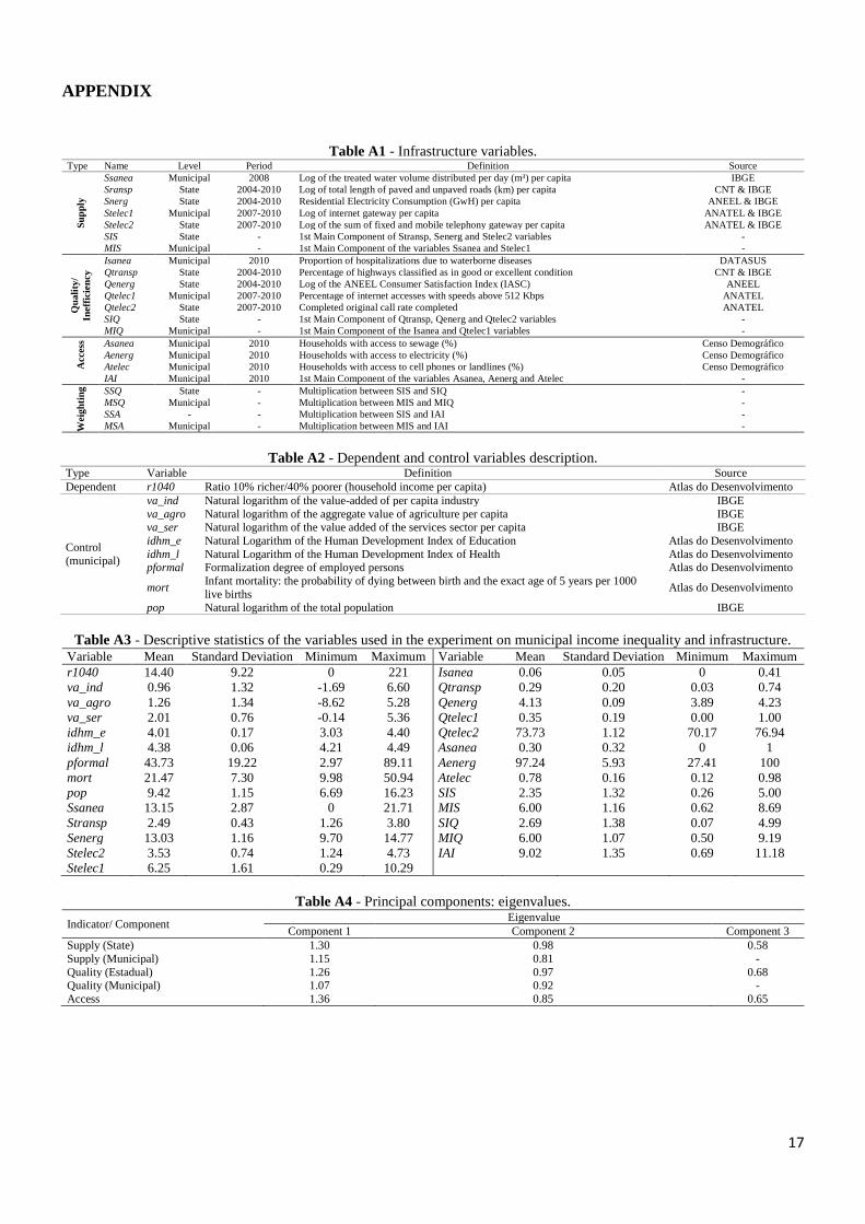
represented by the percentage of households with adequate water supply and sanitary sewage. Table A1 in
Appendix summarizes the infrastructure variables used.
2.4 Composite indices: an application of Principal Component Analysis (PCA)
The indexes are created by Principal Component Analysis according to infrastructure characteristic and its
aggregation. Therefore, for the supply case two indices are calculated, one containing the state-level
variables, and the other with the municipal level variables. The same is true for quality measures. In relation
to access indicators, a single index is created in municipal aggregation. A full description of the method
can be obtained in Dunteman (1989).
Table A4 in Appendix describes the proportion of the variance and its accumulation with the different
components for the indices created. In all cases, we chosen to use those components that had an eigenvalue
greater than one, following the Kaiser’s criterion (Kaiser, 1958). The indices are described in the equations
below:
𝑆𝐼𝑆 = −0,283 ∗ 𝑂𝑡𝑟𝑎𝑛𝑠𝑝 + 0,696 ∗ 𝑂𝑒𝑛𝑒𝑟𝑔 + 0,661 ∗ 𝑂𝑡𝑒𝑙𝑒𝑐2 (1) 𝑀𝐼𝑆 = 0,707 ∗ 𝑂𝑠𝑎𝑛𝑒𝑎 + 0,707 ∗ 𝑂𝑡𝑒𝑙𝑒𝑐1 (2) 𝑆𝐼𝑄 = 0,689 ∗ 𝑄𝑡𝑟𝑎𝑛𝑠𝑝 + 0,663 ∗ 𝑄𝑒𝑛𝑒𝑟𝑔 + 0,291 ∗ 𝑄𝑡𝑒𝑙𝑒𝑐2 (3) 𝑀𝐼𝑄 = −0,707 ∗ 𝑄𝑠𝑎𝑛𝑒𝑎 + 0,707 ∗ 𝑄𝑡𝑒𝑙𝑒𝑐1 (4) 𝐼𝐴𝐼 = 0,503 ∗ 𝐴𝑠𝑎𝑛𝑒𝑎 + 0,593 ∗ 𝐴𝑒𝑛𝑒𝑟𝑔 + 0,628 ∗ 𝐴𝑡𝑒𝑙𝑒𝑐 (5)
The first index created, named State Infrastructure Supply Index (SIS), condenses the information about
power, telephony and transport state-level variables. According to equation 1, power and telephony
indicators have a substantial weight in the index, with a positive sign. The second index, designed
Municipal Infrastructure Supply Index (MIS), added information on sanitation and Internet provision
indicators, which have the same positive weight in the composite index.
A similar procedure is implemented for quality measures, creating the State Infrastructure Quality Index
(SIQ) and the Municipal Infrastructure Quality Index (MIQ), with the same sectors as the supply indexes.
While in the municipal index the variables of sanitation inefficiency and Internet quality have the same
weight, in the state index the variables that hold the highest weight are those linked to the transportation
and power sectors.
Finally, the Infrastructure Access Index (IAI) synthesized information on the variables of access to
electricity, telephony and sanitation. All variables had a significant influence on the index, in such a way
that it represents well the access to infrastructure in the Brazilian municipalities. The composite indicators
described in the equations above are used in the subsequent econometric analysis.
2.5 Hybrid indices: interactions between infrastructure characteristics
The hybrid indexes proposed in this paper seek to simultaneously capture the aggregate effects of access,
quality and infrastructure supply indicators. When analyzing the links between infrastructure and income
inequality, having only one supply indicator is insufficient. In addition, separate analysis of the effects of
provision, access and quality, may not fully reveal the impact of the infrastructure, which is a great
6
challenge in the causality test. Finally, no studies using a hybrid aggregate index that considers both the
infrastructure stock and access were found, in such a way that it becomes a contribution of this study to test
such interactions in the econometric models. Hybrid indices can be described as:
𝑆𝑆𝑄 = 𝑆𝐼𝑆 ∗ 𝑆𝐼𝑄 (6) 𝑀𝑆𝑄 = 𝑀𝐼𝑆 ∗ 𝑀𝐼𝑄 (7) 𝑆𝑆𝐴 = 𝑆𝐼𝑆 ∗ 𝐼𝐴𝐼 (8) 𝑀𝑆𝐴 = 𝑀𝐼𝑆 ∗ 𝐼𝐴𝐼 (9)
In equations 6 and 7 the interactive indices are described between supply and quality both at the state and
municipal level, respectively. In relation to hybrid indicators of quantity and access, two indicators were
also created, both state and municipal level (equations 8 and 9, respectively). This choice was chosen due
to the fact that the telephony and power sector have municipal access indicators, however, their supply is
arranged by state. On the other hand, sanitation access and provision are given at the municipal level, and
an interaction at this level is necessary. The same procedure is done for the disaggregated variables. The
multiplication between supply and quality is named with the initials S (supply) and Q (quality) (example
SQtransp to the transportation sector), while the interaction between supply and access is named with the
initials S and A (access) (example OAenerg to the power sector).
2.6 Income inequality and control variables
In order to represent income inequality, we use “Ratio 10/40 (r1040),” a measure that compares the average
per capita household income of the individuals belonging to the richest decile of the distribution, with the
average per capita household income of the individuals belonging to the poorer two-fifths of people. The
universe of individuals is limited to those who live in permanent private households.
The control variables are represented by the logarithm of the industrial value added per capita, the logarithm
of the aggregate value of agriculture per capita, the logarithm of the value added of the services sector per
capita, logarithm of the education human development index, logarithm of health human development
index, formalization degree of employed persons, rate of infant mortality and the logarithm of total
population. All control variables, as well as the dependent variable, are from the year 2010.2 Table A2 in
Appendix summarizes this group of variables, while Table A3 describes the descriptive statistics of the
variables used in the work.
3. INFRASTRUCTURE EFFECTS ON INCOME INEQUALITY IN A REGIONAL APPROACH:
THE HIERARCHICAL SPATIAL AUTOREGRESSIVE MODEL (HSAR)
Since spatial heterogeneities and dependencies patterns can coexist, it is necessary to treat these two types
of problem together. A model that solves such difficulties is the hierarchical spatial autoregressive model
(HSAR), proposed by Dong and Harris (2014). According to the authors, the purposes of HSAR are: i) to
avoid the “ecological fallacy,” which occurs when transferring relations between variables on an aggregate
scale for individuals; ii) to avoid the “atomistic fallacy,” when correlations between variables are
investigated exclusively at individual level, without taking into account the context; iii) investigate and
quantify contextual effects; and iv) provide better estimates of model parameters and their standard errors
in the presence of group effects.
The motivation of Dong and Harris (2014) in HSAR elaboration was linked to the inability of conventional
hierarchical models to deal with spatial issues that went beyond group heterogeneity. According to the
authors, classical hierarchical models would be able to treat the so-called “vertical group dependence” (or
spatial heterogeneity at the macro level), which occurs when lower level units are similar, since they absorb
identical group effects. However, such models fail to treat the so-called “horizontal group dependence” (or
spatial autocorrelation), characterized by interactions and spillovers that occur due to geographic proximity.
7
The HSAR model, by including the hierarchical data, provides more efficient and accurate estimates for
the regression coefficients. In addition, it provides more correct estimates of the intensity of spatial
interaction at the lower level, separating it from the measurement of regional effects, with which it can be
confused. In this sense, the HSAR model simultaneously integrates spatial autoregressive processes (SAR)
for both the response variable and the upper level residues within a classical hierarchical approach. The key
feature of the SAR process is that it allows the observed values of a dependent variable y in a particular
locality to be directly dependent to the values observed in neighboring locations (or spatial lag of y),
providing both specification and measurement of interaction effects (or spatial spillovers) (LeSage & Pace,
2009). HSAR model specification follows as:
𝑦 = 𝜌𝑊𝑦 + 𝑋𝛽 + 𝑍𝛾 + ∆𝜃 + 𝜀 (10)
𝜃 = 𝜆𝑀𝜃 + 𝑢
Δ = [
𝑙1 0 ⋯ 00 𝑙2 … ⋮… … … …0 0 ⋯ 𝑙𝑗
]
Where y is a column vector N × 1 of the dependent variable values; ρ is the level 1 spatial autoregressive
parameter; W is the spatial weights matrix at municipal level; X is a matrix N × K of independent variables
at the level one; β is a matrix K × 1 of regression coefficients at the municipal level; Z is an N × P matrix
of level two variables; γ is the vector P × 1 of corresponding coefficients of level two; Δ is a diagonal block
matrix N × J with column vectors of ones; and ε is a level one random error term, distributed as 𝑁(0, 𝜎𝑒2).
The vector J × 1 of level two residuals, 𝜃[𝜃1, 𝜃2, … , 𝜃𝑗], represents contextual random effects. The residuals
u are distributed as 𝑁(0, 𝜎𝑢2), and it is assumed that they are independent of ε. Similar to W, M is a
normalized spatial weights matrix at level two, while the parameter λ measures the intensity of spatial
interactions at state level. Finally, specified as a SAR process, the covariance matrix for θ is 𝑐𝑜𝑣(𝜃) =𝜎𝑢
2(𝐵′𝐵)−1, where 𝐵 = 𝐼𝐽 − 𝜆𝑀. As a consequence, the distribution of θ is multivariate
normal, 𝜃~𝑁(0, 𝜎𝑢2(𝐵′𝐵)−1).
The spatial multipliers ρ (Corrado & Fingleton, 2012) and λ indicate nothing more than that spatial
dependence process can have causes such as: i) spatial externalities coming from explanatory variables; ii)
spatial externalities coming from not observed factors; and iii) a feedback or diffusion effect on y; in other
words, some unobserved spatial factor that is captured in the error term. Since there are spatial interaction
effects, a variation in some independent variable in municipality i has a direct effect on municipality i and
an indirect effect on other municipalities. The same is true for a variation in a state-level independent
variable. The direct, indirect and total effects calculation methods can be seen in Dong and Harris (2014).
HSAR model estimation is implemented through a Bayesian simulation approach using Markov Chain
Monte Carlo (MCMC) algorithms.
4. RESULTS AND DISCUSSION
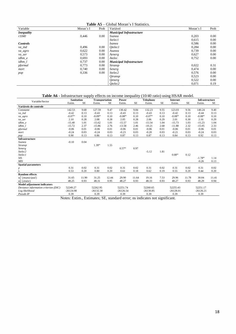
The first practical step is to test the existence of global spatial autocorrelation using Global Moran’s I
statistic.3 As described in Table A5 in Appendix, we can reject the null hypothesis that there is no spatial
autocorrelation in all the variables analyzed, except for transportation supply and telephony quality.
However, the Moran’s I statistic is purely global, thus not allowing us to determine possible clusters and
spatial outliers between the municipalities. Local measurements of spatial autocorrelation are more
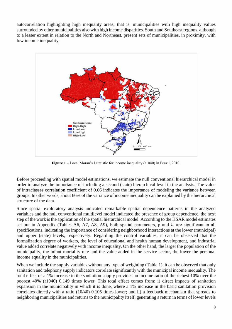
adequate for this type of inference. Figure 1 graphically depicts Local Moran’s I statistic for the income
inequality measure. The map includes municipal values for the Moran Scatterplot that were statistically
significant at the 5% level.
It can be seen from Figure 1 that there are clusters for income inequality. Without great details, Brazil can
practically be divided in two. North and Northeast regions have large clusters of positive spatial
8
autocorrelation highlighting high inequality areas, that is, municipalities with high inequality values
surrounded by other municipalities also with high income disparities. South and Southeast regions, although
to a lesser extent in relation to the North and Northeast, present sets of municipalities, in proximity, with
low income inequality.
Figure 1 – Local Moran’s I statistic for income inequality (r1040) in Brazil, 2010.
Before proceeding with spatial model estimations, we estimate the null conventional hierarchical model in
order to analyze the importance of including a second (state) hierarchical level in the analysis. The value
of intraclasses correlation coefficient of 0.66 indicates the importance of modeling the variance between
groups. In other words, about 66% of the variance of income inequality can be explained by the hierarchical
structure of the data.
Since spatial exploratory analysis indicated remarkable spatial dependence patterns in the analyzed
variables and the null conventional multilevel model indicated the presence of group dependence, the next
step of the work is the application of the spatial hierarchical model. According to the HSAR model estimates
set out in Appendix (Tables A6, A7, A8, A9), both spatial parameters, ρ and λ, are significant in all
specifications, indicating the importance of considering neighborhood interactions at the lower (municipal)
and upper (state) levels, respectively. Regarding the control variables, it can be observed that the
formalization degree of workers, the level of educational and health human development, and industrial
value added correlate negatively with income inequality. On the other hand, the larger the population of the
municipality, the infant mortality rate and the value added in the service sector, the lower the personal
income equality in the municipalities.
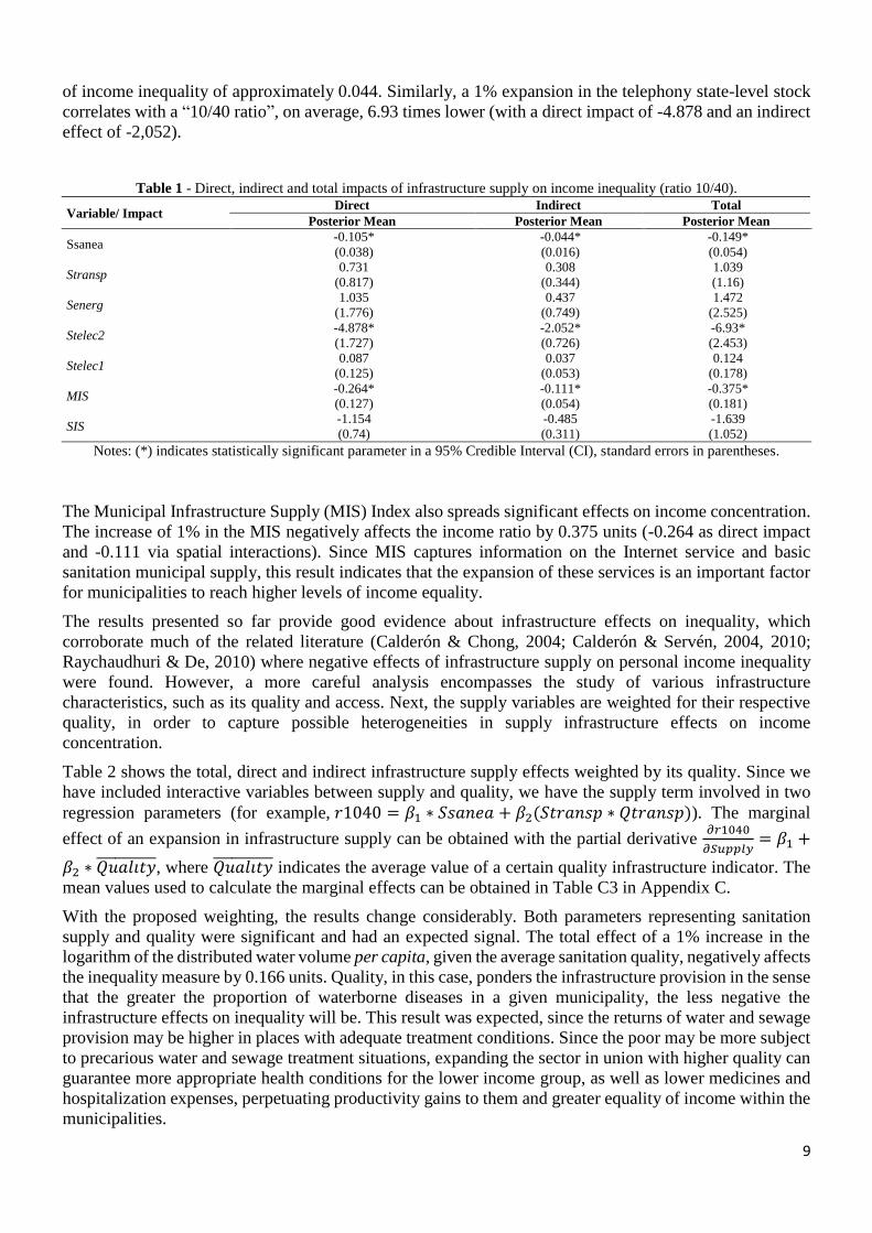
When we include the supply variables without any type of weighting (Table 1), it can be observed that only
sanitation and telephony supply indicators correlate significantly with the municipal income inequality. The
total effect of a 1% increase in the sanitation supply provides an income ratio of the richest 10% over the
poorest 40% (r1040) 0.149 times lower. This total effect comes from: i) direct impacts of sanitation
expansion in the municipality in which it is done, where a 1% increase in the basic sanitation provision
correlates directly with a ratio (10/40) 0.105 times lower; and ii) a feedback mechanism that spreads to
neighboring municipalities and returns to the municipality itself, generating a return in terms of lower levels
9
of income inequality of approximately 0.044. Similarly, a 1% expansion in the telephony state-level stock
correlates with a “10/40 ratio”, on average, 6.93 times lower (with a direct impact of -4.878 and an indirect
effect of -2,052).
Table 1 - Direct, indirect and total impacts of infrastructure supply on income inequality (ratio 10/40).
Variable/ Impact Direct Indirect Total
Posterior Mean Posterior Mean Posterior Mean
Ssanea -0.105* -0.044* -0.149*
(0.038) (0.016) (0.054)
Stransp 0.731 0.308 1.039
(0.817) (0.344) (1.16)
Senerg 1.035 0.437 1.472
(1.776) (0.749) (2.525)
Stelec2 -4.878* -2.052* -6.93*
(1.727) (0.726) (2.453)
Stelec1 0.087 0.037 0.124
(0.125) (0.053) (0.178)
MIS -0.264* -0.111* -0.375*
(0.127) (0.054) (0.181)
SIS -1.154 -0.485 -1.639
(0.74) (0.311) (1.052)
Notes: (*) indicates statistically significant parameter in a 95% Credible Interval (CI), standard errors in parentheses.
The Municipal Infrastructure Supply (MIS) Index also spreads significant effects on income concentration.
The increase of 1% in the MIS negatively affects the income ratio by 0.375 units (-0.264 as direct impact
and -0.111 via spatial interactions). Since MIS captures information on the Internet service and basic
sanitation municipal supply, this result indicates that the expansion of these services is an important factor
for municipalities to reach higher levels of income equality.
The results presented so far provide good evidence about infrastructure effects on inequality, which
corroborate much of the related literature (Calderón & Chong, 2004; Calderón & Servén, 2004, 2010;
Raychaudhuri & De, 2010) where negative effects of infrastructure supply on personal income inequality
were found. However, a more careful analysis encompasses the study of various infrastructure
characteristics, such as its quality and access. Next, the supply variables are weighted for their respective
quality, in order to capture possible heterogeneities in supply infrastructure effects on income
concentration.
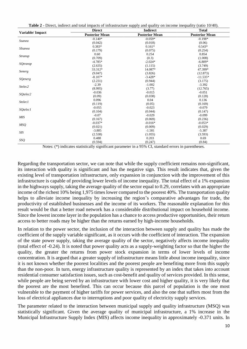
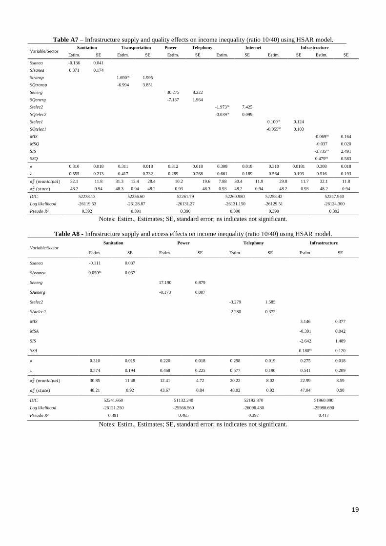
Table 2 shows the total, direct and indirect infrastructure supply effects weighted by its quality. Since we
have included interactive variables between supply and quality, we have the supply term involved in two
regression parameters (for example, 𝑟1040 = 𝛽1 ∗ 𝑆𝑠𝑎𝑛𝑒𝑎 + 𝛽2(𝑆𝑡𝑟𝑎𝑛𝑠𝑝 ∗ 𝑄𝑡𝑟𝑎𝑛𝑠𝑝)). The marginal
effect of an expansion in infrastructure supply can be obtained with the partial derivative 𝜕𝑟1040
𝜕𝑆𝑢𝑝𝑝𝑙𝑦= 𝛽1 +
𝛽2 ∗ 𝑄𝑢𝑎𝑙𝑖𝑡𝑦̅̅ ̅̅ ̅̅ ̅̅ ̅̅ , where 𝑄𝑢𝑎𝑙𝑖𝑡𝑦̅̅ ̅̅ ̅̅ ̅̅ ̅̅ indicates the average value of a certain quality infrastructure indicator. The
mean values used to calculate the marginal effects can be obtained in Table C3 in Appendix C.
With the proposed weighting, the results change considerably. Both parameters representing sanitation
supply and quality were significant and had an expected signal. The total effect of a 1% increase in the
logarithm of the distributed water volume per capita, given the average sanitation quality, negatively affects
the inequality measure by 0.166 units. Quality, in this case, ponders the infrastructure provision in the sense
that the greater the proportion of waterborne diseases in a given municipality, the less negative the
infrastructure effects on inequality will be. This result was expected, since the returns of water and sewage
provision may be higher in places with adequate treatment conditions. Since the poor may be more subject
to precarious water and sewage treatment situations, expanding the sector in union with higher quality can
guarantee more appropriate health conditions for the lower income group, as well as lower medicines and
hospitalization expenses, perpetuating productivity gains to them and greater equality of income within the
municipalities.
10
Table 2 - Direct, indirect and total impacts of infrastructure supply and quality on income inequality (ratio 10/40).
Variable/ Impact Direct Indirect Total
Posterior Mean Posterior Mean Posterior Mean
Ssanea -0.140* -0.059* -0.198*
(0.042) (0.018) (0.06)
SIsanea 0.383* 0.161* 0.543* (0.179) (0.075) (0.254)
Stransp 0.60 0.254 0.854
(0.709) (0.3) (1.008)
SQtransp -4.785* -2.024* -6.809*
(2.635) (1.115) (3.749)
Senerg 33.312* 14.087* 47.399* (9.047) (3.826) (12.873)
SQenerg -8.107* -3.428* -11.535*
(2.231) (0.944) (3.175)
Stelec2 -2.39 -1.002 -3.392
(8.995) (3.77) (12.765)
SQtelec2 -0.036 -0.015 -0.051 (0.09) (0.038) (0.128)
Stelec1 0.096 0.04 0.136
(0.119) (0.05) (0.169)
SQtelec1 -0.055 -0.023 -0.079
(0.104) (0.044) (0.147)
MIS -0.07 -0.029 -0.099
(0.167) (0.069) (0.236)
MSQ -0.037* -0.016* -0.053*
(0.021) (0.009) (0.029)
SIS -3.805 -1.581 -5.387
(2.538) (1.055) (3.593)
SSQ 0.488 0.203 0.69
(0.594) (0.247) (0.84)
Notes: (*) indicates statistically significant parameter in a 95% CI, standard errors in parentheses.
Regarding the transportation sector, we can note that while the supply coefficient remains non-significant,
its interaction with quality is significant and has the negative sign. This result indicates that, given the
existing level of transportation infrastructure, only expansion in conjunction with the improvement of this
infrastructure is capable of providing lower levels of income inequality. The total effect of a 1% expansion
in the highways supply, taking the average quality of the sector equal to 0.29, correlates with an appropriate
income of the richest 10% being 1,975 times lower compared to the poorest 40%. The transportation quality
helps to alleviate income inequality by increasing the region’s comparative advantages for trade, the
productivity of established businesses and the income of its workers. The reasonable explanation for this
result would be that a better road network has a considerable distributional impact on household income.
Since the lowest income layer in the population has a chance to access productive opportunities, their return
access to better roads may be higher than the returns earned by high-income households.
In relation to the power sector, the inclusion of the interaction between supply and quality has made the
coefficient of the supply variable significant, as it occurs with the coefficient of interaction. The expansion
of the state power supply, taking the average quality of the sector, negatively affects income inequality
(total effect of -0.24). It is noted that power quality acts as a supply-weighting factor so that the higher the
quality, the greater the returns from power stock expansion in terms of lower levels of income
concentration. It is argued that a greater supply of infrastructure means little about income inequality, since
it is not known whether the poorest localities and the poorest people are benefiting more from this supply
than the non-poor. In turn, energy infrastructure quality is represented by an index that takes into account
residential consumer satisfaction issues, such as cost-benefit and quality of services provided. In this sense,
while people are being served by an infrastructure with lower cost and higher quality, it is very likely that
the poorest are the most benefited. This can occur because this parcel of population is the one most
vulnerable to the payment of higher tariffs for power services, and also the one that suffers most from the
loss of electrical appliances due to interruptions and poor quality of electricity supply services.
The parameter related to the interaction between municipal supply and quality infrastructure (MSQ) was
statistically significant. Given the average quality of municipal infrastructure, a 1% increase in the
Municipal Infrastructure Supply Index (MIS) affects income inequality in approximately -0.371 units. In
11
this case, the importance of the expansion, with quality, of the services of sanitation and Internet is
indicated. These findings corroborate some of the studies found in the literature (Calderón & Chong, 2004;
Calderón & Servén, 2004, 2010; Seneviratne & Sun, 2013), in the sense that infrastructure quality plays an
important role for localities to reach higher levels of income equality. In addition, the explanation given by
Calderón and Chong (2004) that the quantitative link is stronger than the qualitative one is contradictory,
since, in many cases, the beneficial infrastructure supply effect on lower levels of inequality seems to
necessarily result from a joint expansion in terms of supply and quality.
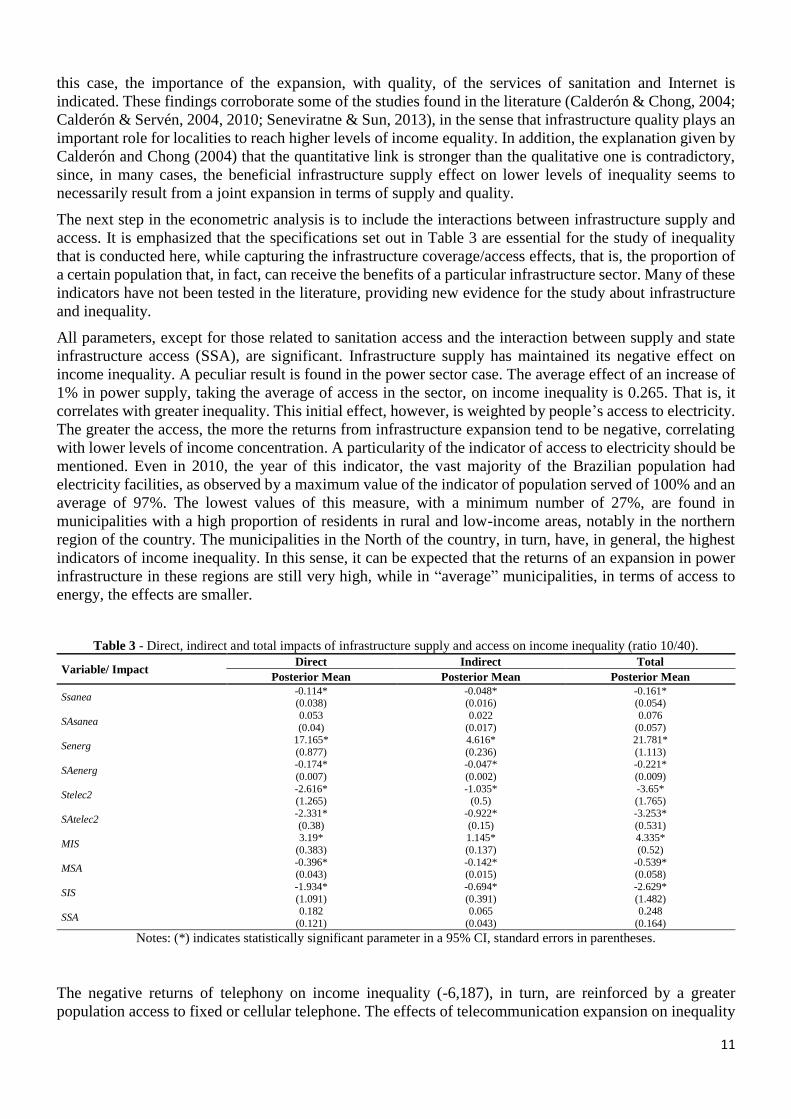
The next step in the econometric analysis is to include the interactions between infrastructure supply and
access. It is emphasized that the specifications set out in Table 3 are essential for the study of inequality
that is conducted here, while capturing the infrastructure coverage/access effects, that is, the proportion of
a certain population that, in fact, can receive the benefits of a particular infrastructure sector. Many of these
indicators have not been tested in the literature, providing new evidence for the study about infrastructure
and inequality.
All parameters, except for those related to sanitation access and the interaction between supply and state
infrastructure access (SSA), are significant. Infrastructure supply has maintained its negative effect on
income inequality. A peculiar result is found in the power sector case. The average effect of an increase of
1% in power supply, taking the average of access in the sector, on income inequality is 0.265. That is, it
correlates with greater inequality. This initial effect, however, is weighted by people’s access to electricity.
The greater the access, the more the returns from infrastructure expansion tend to be negative, correlating
with lower levels of income concentration. A particularity of the indicator of access to electricity should be
mentioned. Even in 2010, the year of this indicator, the vast majority of the Brazilian population had
electricity facilities, as observed by a maximum value of the indicator of population served of 100% and an
average of 97%. The lowest values of this measure, with a minimum number of 27%, are found in
municipalities with a high proportion of residents in rural and low-income areas, notably in the northern
region of the country. The municipalities in the North of the country, in turn, have, in general, the highest
indicators of income inequality. In this sense, it can be expected that the returns of an expansion in power
infrastructure in these regions are still very high, while in “average” municipalities, in terms of access to
energy, the effects are smaller.
Table 3 - Direct, indirect and total impacts of infrastructure supply and access on income inequality (ratio 10/40).
Variable/ Impact Direct Indirect Total
Posterior Mean Posterior Mean Posterior Mean
Ssanea -0.114* -0.048* -0.161* (0.038) (0.016) (0.054)
SAsanea 0.053 0.022 0.076
(0.04) (0.017) (0.057)
Senerg 17.165* 4.616* 21.781*
(0.877) (0.236) (1.113)
SAenerg -0.174* -0.047* -0.221*
(0.007) (0.002) (0.009)
Stelec2 -2.616* -1.035* -3.65* (1.265) (0.5) (1.765)
SAtelec2 -2.331* -0.922* -3.253*
(0.38) (0.15) (0.531)
MIS 3.19* 1.145* 4.335*
(0.383) (0.137) (0.52)
MSA -0.396* -0.142* -0.539* (0.043) (0.015) (0.058)
SIS -1.934* -0.694* -2.629*
(1.091) (0.391) (1.482)
SSA 0.182 0.065 0.248
(0.121) (0.043) (0.164)
Notes: (*) indicates statistically significant parameter in a 95% CI, standard errors in parentheses.
The negative returns of telephony on income inequality (-6,187), in turn, are reinforced by a greater
population access to fixed or cellular telephone. The effects of telecommunication expansion on inequality
12
are enhanced while more individuals have the means to use the services. Since there is ample telephony
coverage in a given municipality, more people, including the poor, can benefit from better productive
opportunities, media, access to information and social interactions through telephony.
The State Infrastructure Supply Index (SIS) has a direct impact on inequality (-2.63), so that the higher the
state supply, the lower the levels of municipal income concentration tend to be. Finally, a 1% change in the
Municipal Infrastructure Supply Index (MIS), taking the average of the Infrastructure Access Index (IAI),
generates a negative effect of 0.52 on the “10/40 Ratio.” The results of the composite indices provide strong
evidence that infrastructure affects inequality when more people actually access these infrastructures, rather
than when such infrastructures have a greater degree of supply. In this sense, the theoretical argument made
by Straub (2008) and Calderón and Servén (2014) is corroborated in that it is imperative to include variables
of access and quality of infrastructure to better explain their relations with issues such as inequality and
poverty.
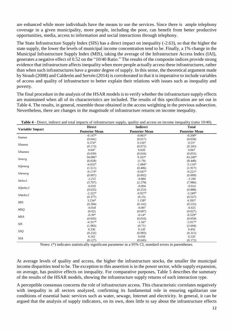
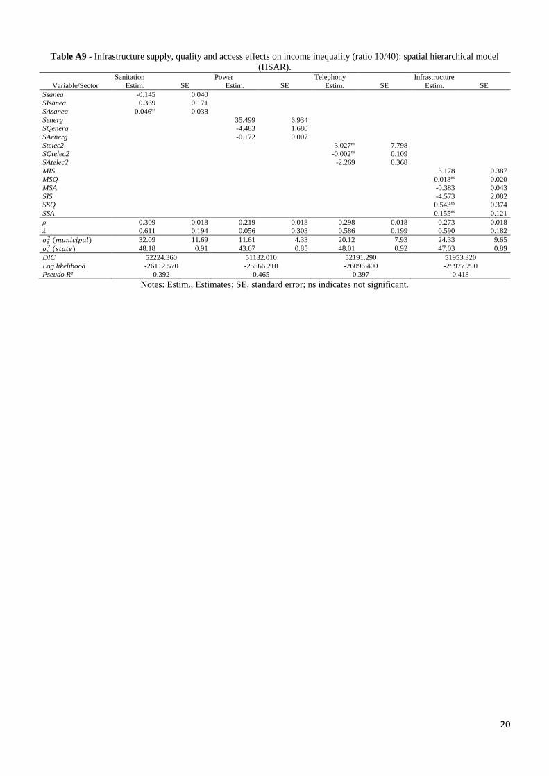
The final procedure in the analysis of the HSAR models is to verify whether the infrastructure supply effects
are maintained when all of its characteristics are included. The results of this specification are set out in
Table 4. The results, in general, resemble those obtained in the access weighting in the previous subsection.
Nevertheless, there are changes in the magnitude of infrastructure returns on income inequality.
Table 4 - Direct, indirect and total impacts of infrastructure supply, quality and access on income inequality (ratio 10/40).
Variable/ Impact Direct Indirect Total
Posterior Mean Posterior Mean Posterior Mean
Ssanea -0.147* -0.061* -0.208*
(0.041) (0.017) (0.058)
SIsanea 0.374* 0.156* 0.53* (0.173) (0.072) (0.245)
SAsanea 0.047 0.020 0.067
(0.039) (0.016) (0.055)
Senerg 34.086* 9.163* 43.249*
(6.658) (1.79) (8.448)
SQenerg -4.032* -1.084* -5.116* (1.511) (0.406) (1.917)
SAenerg -0.174* -0.047* -0.221*
(0.007) (0.002) (0.009)
Stelec2 -2.215 -0.884 -3.100
(5.707) (2.278) (7.986)
SQtelec2 -0.010 -0.004 -0.014 (0.635) (0.253) (0.888)
SAtelec2 -2.322* -0.927* -3.249*
(0.377) (0.15) (0.527)
MIS 3.234* 1.158* 4.392*
(0.394) (0.141) (0.535)
MSQ -0.018 -0.007 -0.025 (0.02) (0.007) (0.027)
MSA -0.39* -0.14* -0.529*
(0.043) (0.016) (0.059)
SIS -4.357* -1.56* -5.917*
(1.983) (0.71) (2.694)
SSQ 0.336 0.120 0.456
(0.232) (0.083) (0.315)
SSA 0.162 0.058 0.220
(0.127) (0.045) (0.172)
Notes: (*) indicates statistically significant parameter in a 95% CI, standard errors in parentheses.
At average levels of quality and access, the higher the infrastructure stocks, the smaller the municipal
income disparities tend to be. The exception to this assertion is in the power sector, while supply expansion,
on average, has positive effects on inequality. For comparative purposes, Table 5 describes the summary
of the results of the HSAR models, showing the infrastructure supply returns of each interaction type.
A perceptible consensus concerns the role of infrastructure access. This characteristic correlates negatively
with inequality in all sectors analyzed, confirming its fundamental role in ensuring egalitarian use
conditions of essential basic services such as water, sewage, Internet and electricity. In general, it can be
argued that the analysis of supply indicators, on its own, does little to say about the infrastructure effects
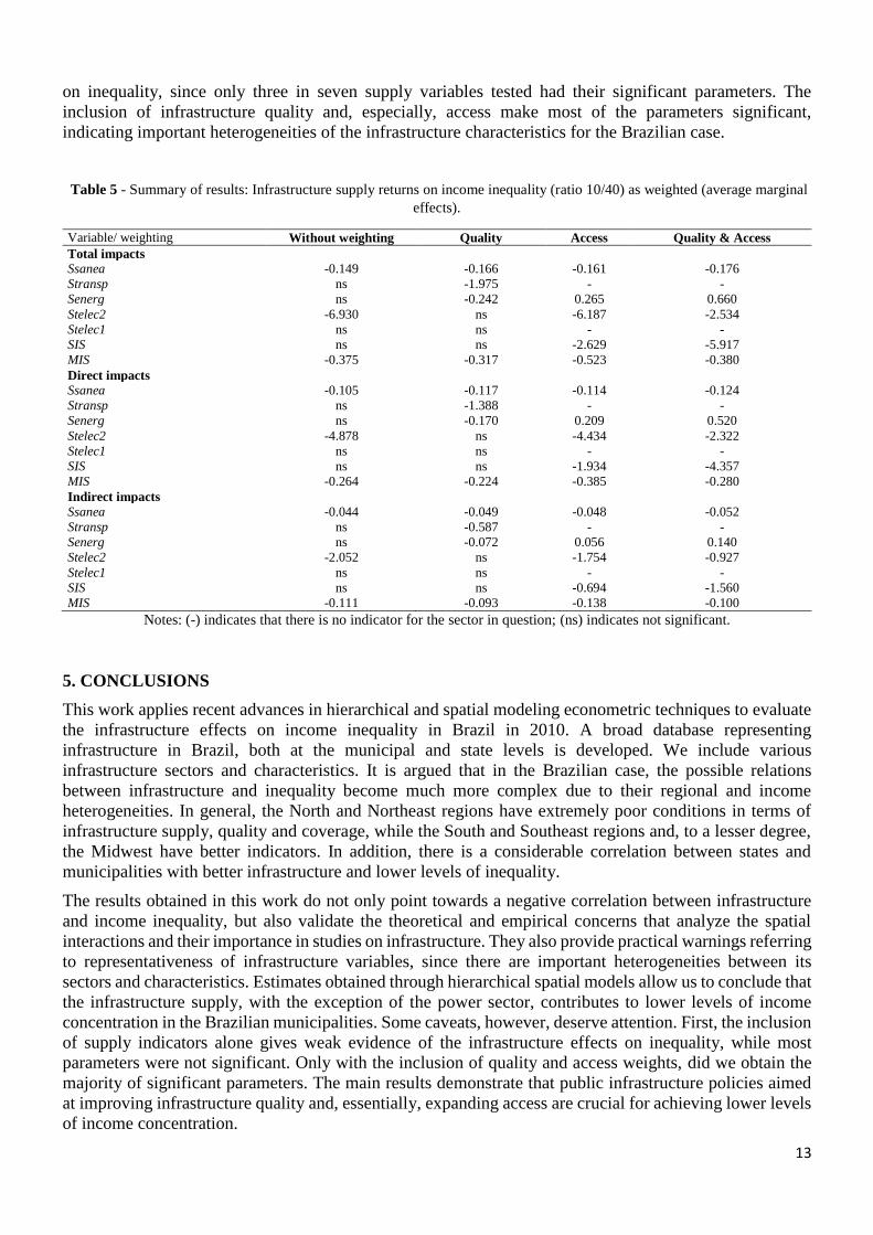
13
on inequality, since only three in seven supply variables tested had their significant parameters. The
inclusion of infrastructure quality and, especially, access make most of the parameters significant,
indicating important heterogeneities of the infrastructure characteristics for the Brazilian case.
Table 5 - Summary of results: Infrastructure supply returns on income inequality (ratio 10/40) as weighted (average marginal
effects).
Variable/ weighting Without weighting Quality Access Quality & Access
Total impacts
Ssanea -0.149 -0.166 -0.161 -0.176
Stransp ns -1.975 - -
Senerg ns -0.242 0.265 0.660
Stelec2 -6.930 ns -6.187 -2.534
Stelec1 ns ns - -
SIS ns ns -2.629 -5.917
MIS -0.375 -0.317 -0.523 -0.380
Direct impacts
Ssanea -0.105 -0.117 -0.114 -0.124
Stransp ns -1.388 - -
Senerg ns -0.170 0.209 0.520
Stelec2 -4.878 ns -4.434 -2.322
Stelec1 ns ns - -
SIS ns ns -1.934 -4.357
MIS -0.264 -0.224 -0.385 -0.280
Indirect impacts
Ssanea -0.044 -0.049 -0.048 -0.052
Stransp ns -0.587 - -
Senerg ns -0.072 0.056 0.140
Stelec2 -2.052 ns -1.754 -0.927
Stelec1 ns ns - -
SIS ns ns -0.694 -1.560
MIS -0.111 -0.093 -0.138 -0.100
Notes: (-) indicates that there is no indicator for the sector in question; (ns) indicates not significant.
5. CONCLUSIONS
This work applies recent advances in hierarchical and spatial modeling econometric techniques to evaluate
the infrastructure effects on income inequality in Brazil in 2010. A broad database representing
infrastructure in Brazil, both at the municipal and state levels is developed. We include various
infrastructure sectors and characteristics. It is argued that in the Brazilian case, the possible relations
between infrastructure and inequality become much more complex due to their regional and income
heterogeneities. In general, the North and Northeast regions have extremely poor conditions in terms of
infrastructure supply, quality and coverage, while the South and Southeast regions and, to a lesser degree,
the Midwest have better indicators. In addition, there is a considerable correlation between states and
municipalities with better infrastructure and lower levels of inequality.
The results obtained in this work do not only point towards a negative correlation between infrastructure
and income inequality, but also validate the theoretical and empirical concerns that analyze the spatial
interactions and their importance in studies on infrastructure. They also provide practical warnings referring
to representativeness of infrastructure variables, since there are important heterogeneities between its
sectors and characteristics. Estimates obtained through hierarchical spatial models allow us to conclude that
the infrastructure supply, with the exception of the power sector, contributes to lower levels of income
concentration in the Brazilian municipalities. Some caveats, however, deserve attention. First, the inclusion
of supply indicators alone gives weak evidence of the infrastructure effects on inequality, while most
parameters were not significant. Only with the inclusion of quality and access weights, did we obtain the
majority of significant parameters. The main results demonstrate that public infrastructure policies aimed
at improving infrastructure quality and, essentially, expanding access are crucial for achieving lower levels
of income concentration.
14
In order to understand the dynamic mechanisms of infrastructure interaction and income inequality in space
and time, panel data models need to be specified and interpreted in future research. Due to the unavailability
of data, this work was limited to cross-section analysis. In addition, we do not address possible problems
of endogeneity between infrastructure and income inequality.
NOTES
1. Both Internet and telephony indicators represent the physical or logical means by which a user is
connected to a telecommunications network (ANATEL, 2012). Therefore, these indicators capture the
telecommunications provision to the total population, including people and firms.
2. The variables used are available for municipal disaggregation only in the Demographic Census prepared
by IBGE (2010). However, since most of the infrastructure variables used are not available for the period
preceding to the year 2000, a temporal analysis was not feasible.
3. To create spatial lags, first-order queen type matrices are created for each hierarchical level. It is the most
commonly matrix used in space econometric studies. Therefore, both W (municipal) and M (state) matrices
are constructed by contiguity, where states/municipalities that have a common border are considered
neighbors.
REFERENCES
ABDID, Associação Brasileira da Infraestrutura e Indústrias de Base. As Particularidades Do Investimento
Em Infraestrutura. Textos para discussão - nº 1 - ano 1, 2018.
ALI, I.; PERNIA, E. M. Infrastructure and poverty reduction: What is the connection? ERD Policy Brief
No. 13, Economics and Research Department, Asian Development Bank, Manila, 2003.
ANATEL, Agência Nacional de Telecomunicações. Acessos: Telefonia Fixa, Telefonia Móvel, Banda
Larga Fixa. Disponível em www.anatel.gov.br/dados, acesso em agosto de 2018.
_____. Qualidade dos Serviços. Disponível em < http://www.anatel.gov.br/dados/controle-de-qualidade>,
acesso em agosto de 2018.
ANEEL, Agência Nacional de Energia Elétrica. Acesso à informação, Dados Abertos, Geração. Disponível
em < http://www.aneel.gov.br/dados/geracao>, acesso em agosto de 2018.
_____. Índice ANEEL de Satisfação do Consumidor (IASC). Disponível em <
http://www.aneel.gov.br/indice-aneel-satisfacao-consumidor>, acesso em agosto de 2018.
ARBUÉS, P, BAÑOS, J. F., Mayor M. The spatial productivity of transportation
infrastructure. Transportation Research Part A 75 (2015) 166–177, 2015.
ASCHAUER, D. “Is public expenditure productive?” Journal of Monetary
Economics, 23(2), 177-200, 1989.
BAJAR, Sumedha; RAJEEV, Meenakshi. The impact of infrastructure provisioning on inequality:
evidence from India. International Labour Office, Global Labour University (GLU), 2015, 35 p.
(Global Labour University working paper; No. 35), 2015.
BANERJEE, A. Who is getting the public goods in India? Some evidence and some
speculation. In BASU, K. (ed.), India's Emerging Economy: Performance and Prospects in the
1990’s and beyond. Cambridge, MIT Press, 2004.
BRAKMAN, S., GARRETSON, H. & C. VAN MARREWIJK. “Locational competition and
agglomeration: The role of government spending,” CESifo Working Paper
775, 2002.
15
CALDERÓN, C.; CHONG, A. Volume and Quality of Infrastructure and the
Distribution of Income: An Empirical Investigation." Review of Income and
Wealth 50, 87-105, 2004.
CALDERÓN, C.; SERVÉN, L. The effects of infrastructure development on growth
and income distribution, World Bank Policy Research Working Paper 3400, 2004.
_____. Infrastructure and economic development in Sub-Saharan Africa”, Journal of African Economies
19(S1), 13-87, 2010.
_____. Infrastructure, Growth, and Inequality: An Overview. World Bank Policy Research Working Paper
No. 7034. The World Bank, 2014.
CALDERÓN, C., MORAL-BENITO, E., SERVÉN, L. Is infrastructure capital productive? A dynamic
heterogeneous approach. J. Appl. Econ. http://dx.doi.org/10.1002/jae.2373, 2014.
CHAKAMERA, C., ALAGIDEDE, P. The nexus between infrastructure (quantity and
Quality) and economic growth in Sub Saharan Africa. International Review of
Applied Economics, DOI: 10.1080/02692171.2017.1355356, 2017.
CONFEDERAÇÃO NACIONAL DOS TRANSPORTES – CNT. Anuário CNT do Transporte 2017.
Disponível em http://anuariodotransporte.cnt.org.br/, acesso em janeiro de 2018.
_____. Pesquisa CNT de Rodovias. Disponível em http://pesquisarodovias.cnt.org.br/, acessado em agosto
de 2018.
CORRADO, L.; FINGLETON, B. Where is the economics in spatial econometrics? Journal of Regional
Science, 52(2):210–239, 2012.
COSCI, S.; MIRRA, L. A spatial analysis of growth and convergence in Italian
provinces: the role of road infrastructure, Regional Studies, DOI:
10.1080/00343404.2017.1334117, 2017.
DEL BO, C.F.; FLORIO, M. Infrastructure and Growth in the European Union: An
Empirical Analysis at the Regional Level in a Spatial Framework. Università
degli Studi, Milano. Working Paper n. 2008-37, 2008.
_____. Infrastructure and growth in a spatial framework:
evidence from the EU regions. Eur. Plan. Stud. 20 (8), 1393–1414, 2012.
DONG, G.; HARRIS, R. J. Spatial autoregressive models for geographically hierarchical data structures.
Geographical Analysis, 47, 173–191, 2014.
DONG, G; HARRIS, R. J.; JONES, K.; YU, J. Multilevel modelling with spatial interaction effects with
application to an emerging land market in Beijing, China. PLoS ONE 10 (6): e0130761. DOI:
10.1371/journal.pone.0130761, 2015.
DUNTEMAN, G.H. (1989). Principal Components Analysis . Beverly Hills:Sage.
FAN, S.; ZHANG, X. Growth, Inequality, and Poverty in Rural China: The Role of Public Investments’,
Research Report 125. Washington DC: IFPRI, 2002.
HOOPER, E.; PETERS, S.; PINTUS, P. A. To What Extent Can Long-Term Investment in Infrastructure
Reduce Inequality? Banque de France Working Paper #624, 2017.
IBGE - Instituto Brasileiro de Geografia e Estatística. Plano Nacional de Saneamento Básico. Rio de
Janeiro, IBGE, 2008.
_____. Censo Demográfico. Rio de Janeiro, IBGE, 2010.
KAISER, H. F. The varimax criterion for analytic rotation in factor analysis. Psychometrika, v. 23, n. 3.p.
187-200, 1958.
16
KHANDKER, S.; G. KOOLWAL. Are pro-growth policies pro-poor? Evidence from Bangladesh. Mimeo,
The World Bank, 2007.
LESAGE, J. P.; PACE, R. K. Introduction to Spatial Econometrics. Boca Raton, FL: CRC Press/Taylor &
Francis, 2009.
MAKMURI, A. Infrastructure and inequality: An empirical evidence from
Indonesia. Economic Journal of Emerging Markets, 9(1) April 2017, 29-39, 2017.
MENDOZA, V. O. M. Infrastructure Development, Income Inequality and Urban Sustainability in the
People’s Republic of China. ADBI Working Paper 713. Tokyo: Asian Development Bank Institute.
Available: https://www.adb.org/publications/infrastructuredevelopment-income-inequality-and-
urban-sustainability-prc, 2017.
MUNNEL, A. H. Infrastructure investment and economic growth. Journal of Economic
Perspectives, vol. 6, n. 4, p. 189-198.1992.
OTTAVIANO, G. I. P. Infrastructure and economic geography: An overview of theory
and evidence. EIB Papers, ISSN 0257-7755, Vol. 13, Iss. 2, pp. 8-35, 2008.
RAISER, Martin; Clarke, Roland N.; PROCEE, Paul; BRICENO-GARMENDIA, Cecilia M.; KIKONI,
Edith; MUBIRU, Joseph Kizito; VINUELA, Lorena. Back to planning: how to close Brazil's
infrastructure gap in times of austerity. Washington, D.C.: World Bank Group.
RAYCHAUDHURI, A.; DE, P. Trade, infrastructure and income inequality in
selected Asian countries: An empirical analysis. Asia-Pacific Research and
Training Network on Trade Working Paper Series, No. 82, August, 2010.
SENEVIRATNE, D.; SUN, Y. Infrastructure and income distribution in ASEAN-
5: what are the links? IMF Working Paper 13/41, 2013.
SILVA, S. P.; LEITE, L. M. Transbordamentos De Pobreza E Desigualdade Em Minas Gerais: Uma
Análise Espacial Considerando O Efeito Da Fronteira Interestadual. Rev. Econ. NE, Fortaleza, v.
48, n. 3, p. 55-76, jul. /set, 2017.
STRAUB, S. Infrastructure and Growth in Developing Countries: Recent Advances and Research
Challenges. Policy Research Working PapeR 4460, 2008.
_____. Infrastructure and Development: A Critical Appraisal of the Macrolevel Literature. Journal of
Development Studies, Vol. 47, No. 5, 683–708, May, 2011.
STRAUB, S.; TERADA-HAGIWARA, A. Infrastructure and growth in developing Asia.
Asian Development Bank Economics Working Paper Series, (231), 2010.
SWISS, Lead in Speed: Comparing Global Internet Connections, 2011. Disponível em:
<http://blog.nielsen.com/nielsenwire/global/swiss-lead-in-speedcomparing-global-internet-
connections/>. Acesso em janeiro de 2018.
17
APPENDIX
Table A1 - Infrastructure variables. Type Name Level Period Definition Source
Su
pp
ly
Ssanea Municipal 2008 Log of the treated water volume distributed per day (m³) per capita IBGE
Sransp State 2004-2010 Log of total length of paved and unpaved roads (km) per capita CNT & IBGE
Snerg State 2004-2010 Residential Electricity Consumption (GwH) per capita ANEEL & IBGE
Stelec1 Municipal 2007-2010 Log of internet gateway per capita ANATEL & IBGE
Stelec2 State 2007-2010 Log of the sum of fixed and mobile telephony gateway per capita ANATEL & IBGE
SIS State - 1st Main Component of Stransp, Senerg and Stelec2 variables -
MIS Municipal - 1st Main Component of the variables Ssanea and Stelec1 -
Qu
ali
ty/
Ineff
icie
ncy
Isanea Municipal 2010 Proportion of hospitalizations due to waterborne diseases DATASUS
Qtransp State 2004-2010 Percentage of highways classified as in good or excellent condition CNT & IBGE
Qenerg State 2004-2010 Log of the ANEEL Consumer Satisfaction Index (IASC) ANEEL
Qtelec1 Municipal 2007-2010 Percentage of internet accesses with speeds above 512 Kbps ANATEL
Qtelec2 State 2007-2010 Completed original call rate completed ANATEL
SIQ State - 1st Main Component of Qtransp, Qenerg and Qtelec2 variables -
MIQ Municipal - 1st Main Component of the Isanea and Qtelec1 variables -
Access
Asanea Municipal 2010 Households with access to sewage (%) Censo Demográfico
Aenerg Municipal 2010 Households with access to electricity (%) Censo Demográfico
Atelec Municipal 2010 Households with access to cell phones or landlines (%) Censo Demográfico
IAI Municipal 2010 1st Main Component of the variables Asanea, Aenerg and Atelec -
Weig
hti
ng
SSQ State - Multiplication between SIS and SIQ -
MSQ Municipal - Multiplication between MIS and MIQ -
SSA - - Multiplication between SIS and IAI -
MSA Municipal - Multiplication between MIS and IAI -
Table A2 - Dependent and control variables description. Type Variable Definition Source
Dependent r1040 Ratio 10% richer/40% poorer (household income per capita) Atlas do Desenvolvimento
Control
(municipal)
va_ind Natural logarithm of the value-added of per capita industry IBGE
va_agro Natural logarithm of the aggregate value of agriculture per capita IBGE va_ser Natural logarithm of the value added of the services sector per capita IBGE
idhm_e Natural Logarithm of the Human Development Index of Education Atlas do Desenvolvimento
idhm_l Natural Logarithm of the Human Development Index of Health Atlas do Desenvolvimento pformal Formalization degree of employed persons Atlas do Desenvolvimento
mort Infant mortality: the probability of dying between birth and the exact age of 5 years per 1000
live births Atlas do Desenvolvimento
pop Natural logarithm of the total population IBGE
Table A3 - Descriptive statistics of the variables used in the experiment on municipal income inequality and infrastructure. Variable Mean Standard Deviation Minimum Maximum Variable Mean Standard Deviation Minimum Maximum
r1040 14.40 9.22 0 221 Isanea 0.06 0.05 0 0.41
va_ind 0.96 1.32 -1.69 6.60 Qtransp 0.29 0.20 0.03 0.74
va_agro 1.26 1.34 -8.62 5.28 Qenerg 4.13 0.09 3.89 4.23
va_ser 2.01 0.76 -0.14 5.36 Qtelec1 0.35 0.19 0.00 1.00
idhm_e 4.01 0.17 3.03 4.40 Qtelec2 73.73 1.12 70.17 76.94
idhm_l 4.38 0.06 4.21 4.49 Asanea 0.30 0.32 0 1
pformal 43.73 19.22 2.97 89.11 Aenerg 97.24 5.93 27.41 100
mort 21.47 7.30 9.98 50.94 Atelec 0.78 0.16 0.12 0.98
pop 9.42 1.15 6.69 16.23 SIS 2.35 1.32 0.26 5.00
Ssanea 13.15 2.87 0 21.71 MIS 6.00 1.16 0.62 8.69
Stransp 2.49 0.43 1.26 3.80 SIQ 2.69 1.38 0.07 4.99
Senerg 13.03 1.16 9.70 14.77 MIQ 6.00 1.07 0.50 9.19
Stelec2 3.53 0.74 1.24 4.73 IAI 9.02 1.35 0.69 11.18
Stelec1 6.25 1.61 0.29 10.29
Table A4 - Principal components: eigenvalues.
Indicator/ Component Eigenvalue
Component 1 Component 2 Component 3
Supply (State) 1.30 0.98 0.58
Supply (Municipal) 1.15 0.81 -
Quality (Estadual) 1.26 0.97 0.68 Quality (Municipal) 1.07 0.92 -
Access 1.36 0.85 0.65
18
Table A5 – Global Moran’s I Statistics. Variable Moran’s I Prob Variável Moran’s I Prob
Inequality Municipal Infrastructure
r1040 0,446 0.00 Ssanea 0,203 0.00
Stelec1 0,615 0.00
Controls Isanea 0,586 0.00
va_ind 0,496 0.00 Qtelec1 0,284 0.00
va_agro 0,622 0.00 Asanea 0,739 0.00 va_ser 0,573 0.00 Aenerg 0,627 0.00
idhm_e 0,693 0.00 Atelec 0,752 0.00
idhm_l 0,737 0.00 Municipal Infrastructure pformal 0,773 0.00 Stransp 0,022 0.31
mort 0,740 0.00 Senerg 0,474 0.00
pop 0,336 0.00 Stelec2 0,576 0.00
Qtransp 0,523 0.00
Qenerg 0,522 0.00
Qtelec2 0,071 0.19
Table A6 - Infrastructure supply effects on income inequality (10/40 ratio) using HSAR model.
Variable/Sector Sanitation Transportation Power Telephony Internet Infrastructure
Estim. SE Estim. SE Estim. SE Estim. SE Estim. SE Estim. SE
Variáveis de controle
Constante 142.53 9.68 127.59 9.47 130.42 9.84 132.23 9.55 123.03 9.56 140.24 9.40
va_ind -0.42 0.13 -0.43 0.13 -0.43 0.13 -0.43 0.13 -0.42 0.13 -0.44 0.13
va_agro -0.07ns 0.10 -0.09ns 0.10 -0.08ns 0.10 -0.07ns 0.10 -0.08ns 0.10 -0.08ns 0.10
va_ser 2.10 0.28 2.08 0.28 2.05 0.28 2.06 0.29 2.01 0.30 2.16 0.29
idhm_e -15.40 1.01 -15.62 1.01 -15.57 1.01 -15.54 1.04 -15.73 1.03 -15.23 1.04
idhm_l -15.72 2.37 -15.86 2.76 -13.58 2.46 -10.21 2.68 -11.88 2.32 -15.05 2.33
pformal -0.06 0.01 -0.06 0.01 -0.06 0.01 -0.06 0.01 -0.06 0.01 -0.06 0.01
mort -0.24 0.03 -0.24 0.03 -0.23 0.03 -0.20 0.03 -0.21 0.03 -0.24 0.03
pop 0.90 0.13 0.86 0.13 0.87 0.13 0.87 0.13 0.84 0.13 0.92 0.13
Infrastructure
Ssanea -0.10 0.04
Stransp 1.39ns 1.55
Senerg 0.57ns 0.97
Stelec2 -5.12 1.81
Stelec1 0.08ns 0.12
SIS -1.78ns 1.14
MIS -0.26 0.13
Spatial parameters
ρ 0.31 0.02 0.31 0.02 0.31 0.02 0.31 0.02 0.31 0.02 0.31 0.02
λ 0.53 0.20 0.80 0.20 0.61 0.18 0.62 0.19 0.55 0.20 0.44 0.20
Random effects
𝜎𝑒2 (𝑚𝑢𝑛𝑖𝑐𝑖𝑝𝑎𝑙) 31.65 11.90 31.25 12.44 29.90 11.64 19.16 7.53 29.96 11.78 30.04 11.41
𝜎𝑢2 (𝑠𝑡𝑎𝑡𝑒) 48.25 0.93 48.31 0.95 48.27 0.93 48.33 0.93 48.27 0.93 48.29 0.94
Model adjustment indicators
Deviance information criterion (DIC) 52249.27 52262.95 52251.74 52260.65 52255.43 52251.17
Log likelihood -26124.98 -26132.30 -26126.54 -26130.85 -26128.01 -26126.21
Pseudo R² 0.39 0.39 0.39 0.39 0.39 0.39
Notes: Estim., Estimates; SE, standard error; ns indicates not significant.
19
Table A7 – Infrastructure supply and quality effects on income inequality (ratio 10/40) using HSAR model.
Variable/Sector Sanitation Transportation Power Telephony Internet Infrastructure
Estim. SE Estim. SE Estim. SE Estim. SE Estim. SE Estim. SE
Ssanea -0.136 0.041
SIsanea 0.371 0.174
Stransp 1.690ns 1.995
SQtransp -6.994 3.851
Senerg 30.275 8.222
SQenerg -7.137 1.964
Stelec2 -1.973ns 7.425
SQtelec2 -0.039ns 0.099
Stelec1 0.100ns 0.124
SQtelec1 -0.055ns 0.103
MIS -0.069ns 0.164
MSQ -0.037 0.020
SIS -3.735ns 2.491
SSQ 0.479ns 0.583
ρ 0.310 0.018 0.311 0.018 0.312 0.018 0.308 0.018 0.310 0.0181 0.308 0.018
λ 0.555 0.213 0.417 0.232 0.289 0.268 0.661 0.189 0.564 0.193 0.516 0.193
𝜎𝑒2 (𝑚𝑢𝑛𝑖𝑐𝑖𝑝𝑎𝑙) 32.1 11.8 31.3 12.4 28.4 10.2 19.6 7.88 30.4 11.9 29.8 11.7 32.1 11.8
𝜎𝑢2 (𝑠𝑡𝑎𝑡𝑒) 48.2 0.94 48.3 0.94 48.2 0.93 48.3 0.93 48.2 0.94 48.2 0.93 48.2 0.94
DIC 52238.13 52256.60 52261.79 52260.980 52258.42 52247.940
Log likelihood -26119.53 -26128.87 -26131.27 -26131.150 -26129.51 -26124.300
Pseudo R² 0.392 0.391 0.390 0.390 0.390 0.392
Notes: Estim., Estimates; SE, standard error; ns indicates not significant.
Table A8 - Infrastructure supply and access effects on income inequality (ratio 10/40) using HSAR model.
Variable/Sector Sanitation Power Telephony Infrastructure
Estim. SE Estim. SE Estim. SE Estim. SE
Ssanea -0.111 0.037
SAsanea 0.050ns 0.037
Senerg 17.190 0.879
SAenerg -0.173 0.007
Stelec2 -3.279 1.585
SAtelec2 -2.280 0.372
MIS 3.146 0.377
MSA -0.391 0.042
SIS -2.642 1.489
SSA 0.180ns 0.120
ρ 0.310 0.019 0.220 0.018 0.298 0.019 0.275 0.018
λ 0.574 0.194 0.468 0.225 0.577 0.190 0.541 0.209
𝜎𝑒2 (𝑚𝑢𝑛𝑖𝑐𝑖𝑝𝑎𝑙) 30.85 11.48 12.41 4.72 20.22 8.02 22.99 8.59
𝜎𝑢2 (𝑠𝑡𝑎𝑡𝑒) 48.21 0.92 43.67 0.84 48.02 0.92 47.04 0.90
DIC 52241.660 51132.240 52192.370 51960.090
Log likelihood -26121.250 -25566.560 -26096.430 -25980.690
Pseudo R² 0.391 0.465 0.397 0.417
Notes: Estim., Estimates; SE, standard error; ns indicates not significant.
20
Table A9 - Infrastructure supply, quality and access effects on income inequality (ratio 10/40): spatial hierarchical model
(HSAR).
Variable/Sector
Sanitation Power Telephony Infrastructure
Estim. SE Estim. SE Estim. SE Estim. SE
Ssanea -0.145 0.040 SIsanea 0.369 0.171 SAsanea 0.046ns 0.038 Senerg 35.499 6.934 SQenerg -4.483 1.680 SAenerg -0.172 0.007 Stelec2 -3.027ns 7.798 SQtelec2 -0.002ns 0.109 SAtelec2 -2.269 0.368 MIS 3.178 0.387 MSQ -0.018ns 0.020
MSA -0.383 0.043
SIS -4.573 2.082 SSQ 0.543ns 0.374
SSA 0.155ns 0.121
ρ 0.309 0.018 0.219 0.018 0.298 0.018 0.273 0.018
λ 0.611 0.194 0.056 0.303 0.586 0.199 0.590 0.182
𝜎𝑒2 (𝑚𝑢𝑛𝑖𝑐𝑖𝑝𝑎𝑙) 32.09 11.69 11.61 4.33 20.12 7.93 24.33 9.65
𝜎𝑢2 (𝑠𝑡𝑎𝑡𝑒) 48.18 0.91 43.67 0.85 48.01 0.92 47.03 0.89
DIC 52224.360 51132.010 52191.290 51953.320
Log likelihood -26112.570 -25566.210 -26096.400 -25977.290 Pseudo R² 0.392 0.465 0.397 0.418
Notes: Estim., Estimates; SE, standard error; ns indicates not significant.