Embed Size (px)
Citation preview

Infrastructure and FDI:
Evidence from district-level data in India
Rajesh Chakrabarti, Krishnamurthy Subramanian, Sesha Meka and Kuntluru Sudershan1
March 20, 2012
Abstract
Though public infrastructure – physical and financial – is widely believed to play a critical role in
attracting Foreign Direct Investment (FDI), identifying this effect remains a challenge. In this paper,
we use unique data to identify this effect by exploiting purely cross-sectional variation among
approximately 600 districts in India. We examine the effect of infrastructure in 2001 on cumulative
FDI flows into the district during 2002-07. Using panel regressions that include state fixed effects, we
employ a two-pronged identification strategy. First, we test by netting out average (and maximum)
FDI inflows into surrounding districts. Second, we exploit variation among different sectors within a
district depending upon the sector’s propensity to attract FDI. Since our variables vary primarily at
the district level, these tests together control for all omitted variables at the district level. Surprisingly,
we find that FDI inflows remain insensitive to changes in infrastructure till a threshold is reached;
thereafter, FDI inflows increase steeply with an increase in infrastructure. Keywords: Infrastructure, FDI, India, District JEL Code: F3
1 Rajesh Chakrabarti, Krishnamurthy Subramanian and Sesha Sai Ram Meka are from the Indian School of Business, Hyderabad, India and Kuntluru Sudershan is from the Indian Institute of Management, Kozhikode, India. We would like to thank Viral Acharya, Pochiraju Bhimasankaram, Robin Burgess, Amartya Lahiri, Dilip Mookherjee, Kaivan Munshi, Rohini Somanathan, Kannan Srikanth and other participants at the ISB Econ-Finance seminar and the IGC-ISI growth conference, Delhi for their valuable comments and suggestions. Please email Krishnamurthy Subramanian ([email protected]) for any correspondence. All errors are our own.
Infrastructure and FDI:
Evidence from district-level data in India
March 20, 2012
Abstract
Though public infrastructure – physical and financial – is widely believed to play a critical role in
attracting Foreign Direct Investment (FDI), identifying this effect remains a challenge. In this paper,
we use unique data to identify this effect by exploiting purely cross-sectional variation among
approximately 600 districts in India. We examine the effect of infrastructure in 2001 on cumulative
FDI flows into the district during 2002-07. Using panel regressions that include state fixed effects, we
employ a two-pronged identification strategy. First, we test by netting out average (and maximum)
FDI inflows into surrounding districts. Second, we exploit variation among different sectors within a
district depending upon the sector’s propensity to attract FDI. Since our variables vary primarily at
the district level, these tests together control for all omitted variables at the district level. Surprisingly,
we find that FDI inflows remain insensitive to changes in infrastructure till a threshold is reached;
thereafter, FDI inflows increase steeply with an increase in infrastructure. Keywords: Infrastructure, FDI, India, District JEL Code: F3
1
1 Introduction The past three decades have witnessed enormous growth in global diversification by
multinational firms. From 1980 to 2007, FDI inflows worldwide grew by about 14% in real terms
while real GDP growth and exports increased annually only at 3.2% and 7.3% respectively.
Significant chunks of these inflows have been into developing economies, especially the BRIC
economies.1 Between 2000 and 2006, FDI inflows into the BRIC economies grew annually at 41.3%
when compared to 24.1% in the US, which is the single biggest recipient of FDI, and 22.7% in the
EU, which is the largest regional destination. As a result, the inward stock of FDI in the BRIC
countries grew from 8% to 13% of the global stock of FDI. Since MNCs pursue FDI to create
shareholder value by diversifying internationally (Fatemi, 1984, Lins and Servaes, 1999 and Denis et
al. 2002), the localization of FDI to a few countries represents a puzzling aspect of this important
phenomenon. Since the choice of location by MNCs forms an area of inquiry central to international
corporate finance, in this overarching theme, we ask the following question: What is the effect of
public infrastructure – physical and financial – on the choice of FDI location?
Together with trade policies (see Blonigen, 1997 among others) and tax policies (Hartman,
1985 and others), provision of physical and financial infrastructure can be a potent tool for
governments to attract FDI. Despite the obvious importance to academics and policy makers,
empirical consensus on the basic relationship between public infrastructure and FDI remains
surprisingly elusive. Theoretical arguments exhibit a dichotomy as well. While the canonical FDI-
location-choice models (see Martin and Rogers, 1995 and among others) predict that an increase in
infrastructure uniformly increases FDI inflows, recent theoretical work incorporating the intermediate
goods sector into a general equilibrium framework predicts that FDI will be insensitive to any changes
in infrastructure till a threshold is reached (see Haaland and Wooton, 1999 and Kellenberg, 2007).
The disagreement persists because identifying the effect of public infrastructure on FDI
presents empirical challenges. First, accurate and comparable measurements for the level of public
infrastructure are not easily available (see Blonigen, 2005). Second, cross-country comparisons to pin-
point the effect of infrastructure on FDI inflows remain mired in identification problems. Countries
that differ in the provision of infrastructure usually vary on other observed and unobserved
dimensions.2 Furthermore, the level of infrastructure in a country is quite persistent, which leads to
little informative variation over time within a country. Even when the level of infrastructure varies
over time within a country, periods involving significant changes in infrastructure generally coincide
with other structural changes as well.
1 Brazil, Russia, India and China 2 These include differences in abundance of natural resources, availability of cheap and skilled labor, the efficacy of law enforcement and the rule of law, the quality of bureaucracy, corruption, trade and taxation policies as well as market size
2
In this paper, we overcome these challenges by employing a unique dataset of FDI at the
district-level in India to cleanly identify the effect of infrastructure on FDI inflows. India provides an
ideal setting to study this question. First, India is an important constituent of the BRIC economies.
Second, the federal structure in India, where state governments compete with each other to attract
FDI, enables us to identify the effects after accounting for endogenous policy responses to attract FDI.
We find that the impact of public infrastructure – physical and financial – on FDI inflow, though
positive, is essentially non-linear. FDI inflows remain insensitive to improvements in infrastructure
till a threshold is reached; thereafter, FDI inflows increase steeply with an increase in infrastructure.
To identify this effect, we exploit cross-sectional variation in infrastructure and FDI flows
among close to 600 districts in India. We obtain project-level information on FDI from the long-term
Foreign Collaboration (FC) project proposals approved either by the Reserve Bank of India or the
Ministry of Commerce and Industry in the Government of India; FDI regulation in India necessitates
such approvals. Such FC project proposals are collected by the CapEx database of the Centre for
Monitoring Indian Economy (CMIE). The data includes information on the district where the FC
project is located, which is central to our identification strategy. Our data has the advantage of
pertaining to a geographical unit (district) that is not a sub-national policy-making unit. Thus, we can
abstract from the confounding effects due to regional policies through the use of state fixed effects.
Our use of districts also allows us enough observations to power our statistical tests.
Our explanatory variables are obtained from the socio-economic variables collected from
various government sources by “Indian Development Landscape” product of Indicus database. We
use the four different indicators of infrastructure in our data: (i) habitations connected by paved roads;
(ii) households with electricity connections; (iii) households with a telephone connection; and (iv) the
number of scheduled commercial bank branches. While the first three indicators capture the effect of
physical infrastructure, the fourth indicator captures that of financial infrastructure. Two snapshots in
time, in 2001 and in 2008, are available for the Indicus data. Since the FC project data is available
only till 2008, we examine the effect of district-level infrastructure in 2001 on cumulative FDI
inflows into a district over the time period 2002-07. To obtain a single index of infrastructure at the
district-level in 2001, we undertake a principal component analysis using these four variables (see
Chamberlain and Rothschild, 1983; Connor and Korajczyk, 1986 and others). In our case, the first
principal component assigns a positive and almost equal weight to each of the four variables. More
importantly, it explains more than two-thirds of the total variance.
Our empirical setup enables the direction of causation to run from infrastructure to FDI
inflows and not vice-versa. First, we examine the effect of infrastructure in a given district in the year
2001 on FDI inflows over the time period 2002-07. Second, since creating new infrastructure is a
relatively time-consuming process, the infrastructure in Indian districts changes very little during the
3
time period 2001 to 2007,3 which implies that FDI inflows may not have led to changes in
infrastructure. Third, our identification does not rely on any time-series variation that is more likely to
be affected by reverse causality. Instead, we identify the intended effect by exploiting purely cross-
sectional variation among districts within a state.
Figure 1 shows visual plots of the relationship between the level of public infrastructure in a
district in 2001 and the FDI inflows into the district during 2002-07. The figure illustrates a striking
non-linear relationship between district-level infrastructure and FDI inflows. In particular, FDI
inflows remain insensitive to infrastructure till a threshold level of infrastructure is reached;
thereafter, FDI inflows increase steeply with an increase in infrastructure. Furthermore, as preliminary
evidence of this relationship not been driven by district level omitted variables, in Figure 2, we find
that this nonlinear relationship is not obtained between FDI and either of human development,
economic status or crime measured at the district level.
**** Insert Figures 1 and 2 about here ****
We provide preliminary evidence confirming this non-linear relationship using statistical tests
that implement the econometric variant of Figure 1. Specifically, we employ cross-sectional
regressions that include state fixed effects. Since states compete with each other to attract FDI
investment, state-level policies such as tax rates, minimum-wage rates, sops offered to attract FDI are
all endogenous factors affecting FDI investment. Since our sample exhibits variation only in the
cross-section, the state fixed effects enable us to control for all state-level observed and unobserved
factors, thereby enabling us to identify the intended effect purely using within-state variation. Using
regressions that employ a quadratic functional form as well as ones with piecewise linear splines, we
find strong evidence of the non-linear effect observed in Figure 1.
We estimate this effect after controlling for several others determinants of FDI at the district-
level: level of education, health, economic development, population, human development measures
such as empowerment of women, violent crime, GDP per capita, and whether the district is a
metropolitan city are not. These control variables enable us to control for broad determinants of FDI
inflows such as the availability of skilled labor, the wage rates prevailing in a district as well as
demand-side determinants such as economic prosperity.
However, we cannot infer the causal effect of infrastructure on FDI from the above tests
because omitted variables at the district level may be correlated with the level of FDI in a district. For
example, as Coughlin and Segev (2000) and Blonigen et al. (2004) show, FDI inflows into a
particular district may accrue due to agglomeration externalities, i.e. the district attracts FDI inflows
because other neighboring districts are attractive FDI destinations for strictly endogenous reasons.
3 In fact, the correlation between the value of the infrastructure variables in 2001 and those in 2008 equal 0.96, 0.91, 0.88 and 0.99 for Habitations connected by paved roads, Households with electricity connection, Households with telephone, Number of scheduled commercial bank branches respectively.

4
Furthermore, our above results could be driven by unobserved differences in the demand for the
good/service that a multinational enterprise (MNE) caters to through the FC project.
We alleviate these concerns using a two-pronged empirical strategy. First, we use FDI into
surrounding districts to control for the effect of omitted variables. Since neighboring districts take on
almost identical values for the observed variables, they are likely to take on similar values for the
various unobserved factors that affect FDI inflows. Therefore, by netting out the average FDI inflows
into surrounding districts we immunize the effect of all district-level omitted variables. The top-right
plot in Figure 1 provides a visual illustration that the non-linear effect of infrastructure obtained above
carries over to this specification as well. In panel regressions using the difference between FDI
inflows in a district and average FDI inflows into its surrounding districts, we also include a dummy
for any of the surrounding districts being a metropolitan city to control for unobserved determinants
stemming from proximity to a metropolitan city.
We replicate the above tests by netting out the maximum FDI inflow among the surrounding
districts. This test enables us to control for unobserved determinants of FDI in a district using the
most attractive destination among the surrounding districts. In both these set of tests, our results stay
as strong as before, which lead us to confirm that district-level endogenous factors may not be driving
our results. In fact, since our sample exhibits variation only in the cross-section and the tests
employing the surrounding districts resemble a quasi district-fixed-effect, these tests enable us to
more cleanly identify the effect of public infrastructure on FDI inflows.
Second, as our strongest piece of evidence, we exploit variation within a district in the effect
of infrastructure on FDI inflows into different sectors after controlling for all district level effects
using district fixed effects. To proxy a sector’s propensity to attract FDI, we rank sectors at the
national level by the volume of FDI they attract in 2001. We then interact this sector-level FDI
propensity measure with our district-level infrastructure measures and find that within a district the
effect of infrastructure is more pronounced in sectors that have a greater intensity to attract FDI. We
emphasize that these tests control for all omitted variables at the district level and enable us to identify
cleanly the intended effect by exploiting variation among different sectors within a district.
We undertake other robustness tests to rule out various alternative interpretations. First, we
examine whether the level of infrastructure in a district in 2001 has a nonlinear effect on FDI in each
year from 2002 to 2006. In these tests, we also control for the average FDI into surrounding districts
in the previous year as well as the domestic investment in the particular district in the previous year.
We find that the nonlinear effect of infrastructure on FDI is remarkably consistent for each year in the
sample. Second, to examine the possibility that our results are due to lobbying by large MNEs, we
separately run our results for the highest and lowest quartiles in terms of the value of FDI and find our
results to be equally strong for both. Since lobbying by large MNEs are more likely to show up in the
largest FDI projects, these results reassure us that the results may not be just an outcome of lobbying
by large MNEs.

5
In sum, across various tests that progressively relax the assumptions required to identify the
intended effect, we find a robust non-linear effect of public infrastructure on FDI inflows. The
economic magnitude of the effect of public infrastructure on FDI inflows is quite significant. We find
that a one standard deviation increase in infrastructure in a district that has an above median level of
infrastructure within the state increases annual FDI inflows by approximately 8.7%. However, an
increase in the infrastructure in a district that has a below median level of infrastructure within the
state has a negligible effect on its FDI inflows.
Our study contributes to the literature examining the determinants of FDI inflows. Our work
resembles closely that of Antras et al. (2009) who examine the effect of “soft” infrastructure such as
the strength of investor protection and as the cost of financial contracting on MNE activity and FDI
inflows. Their theoretical model predicts that weak investor protection and costly financial frictions
limit the scale of MNE activity; their firm-level evidence supports this thesis. In contrast, we focus on
the effect of “hard” physical infrastructure such as good roads, telephone and electricity connections
and financial infrastructure such as the presence of a commercial bank branch. While Antras et al.
(2009) find a uniform effect of soft infrastructure on FDI inflows, we find that a threshold level of
hard infrastructure is required to attract FDI. These contrasting findings suggest that soft and hard
aspects of infrastructure may have very different roles to play in attracting investment, in general, and
FDI, in particular.
Our key finding of non-linearity in the effect of infrastructure on FDI is particularly relevant
to the ongoing theoretical debate among alternative FDI-location-choice models. The canonical
models (see Martin and Rogers, 1995 and Baldwin and Martin, 2003) predict a uniformly positive
impact while general-equilibrium models (for instance, Haaland and Wooton, 1999 and Kellenberg,
2007) argue, by including an intermediate goods sector, that the effect of infrastructure on FDI will
not manifest till a threshold level of infrastructure is reached. While further investigation needs to be
done to better understand the suitability of our finding in this debate, prima facie, we provide
evidence that seems to provide greater support to the latter class of models.
Apart from the effect of infrastructure, the literature relating to determinants of FDI has
examined factors such as capital controls (see Desai et al., 2006), financial crises (Lipsey, 2001 and
Desai et al., 2008), credit constraints (Manova et al., 2009), exchange rate movements (see Blonigen,
2005 and others), market size, labor cost and political instability (Scaperlanda and Balough, 1983;
Filatotchev et al., 2007; Brouwer et al., 2008). Often these factors interact and complicate the
identification problem. Our use of intra-country variations in FDI flows allows us to abstract from
most of these issues that are essentially national in nature.
Determinants of FDI flows have also been an important part of the finance literature. The role
of lower investment costs and FDI flows has been investigated in Henry (2000). More recently Chari
and Gupta (2008) have looked into the determinants of FDI flows in certain industries in liberalizing
6
economies. Rossi and Volpin (2004) and Baker et al. (2009) have looked at the effects of stock
market valuations on FDI flows.
We are, of course, not the first to study intra-country variation in FDI flows. Several studies
have studied FDI location choice within the USA (see Carlton, 1983; Coughlin et al., 1991; Head et
al., 1994). Among recent studies, some have focused on the regional choices of FDI in China (Head
and Ries, 1996 and Cheng and Kwan, 2000) while others have investigated the phenomenon in
Europe (Scaperlanda and Balough, 1983; Devereux and Griffith, 1998; Cantwell and Iammarino,
2000; Guimaraes et al., 2000; Boudier-Bensebaa, 2005). Our study differs from other intra-country
studies in that often in federal settings, different regions have control over policies that affect the
attractiveness of these regions to FDI. Our use of districts releases us from such concerns since the
federal power structure stops at a higher level, i.e. states, in India and such differences can be
subsumed in the state fixed effects we use in our analysis.
Our findings are quite relevant to the broader FDI literature and policy as well. On the one
hand, our results help to explain why marginal improvements in bottom-rung countries fail to excite
multinational enterprises (MNEs) to enter them (Woodward and Rolfe, 1993; Sethi et al., 2003; Sol
and Kogan, 2007; Rose and Ito, 2008; Sembenelli and Siotis, 2008; Blalock and Simon, 2009; Liu et
al., 2009). On the other hand, the results help explain the spectacular performance of countries like
China in achieving rapid industrialization and economic growth by focusing on pockets of high
infrastructure - the special economic zones (SEZ) approach - rather than by spreading the investment
in infrastructure uniformly across the country.
The next section of the paper describes the data and variables while section 3 describes the
empirical results. Section 4 posits a theoretical explanation for our results. Concluding remarks follow
in Section 5.
2 Data and Proxies In this section, we describe our proxies for district-level FDI inflows and our district-level
measures for the level of public infrastructure.
2.1 District-level FDI data
Our information on FDI comes from the Capital Expenditure (CapEx) database created by the
Center for Monitoring of the Indian Economy (CMIE) (www.cmie.com). CapEx is a unique database
tracking new and ongoing investment activities in India. These are investments in new plants and
machinery. A project enters the CapEx database from the time it is announced till it is commissioned
or abandoned. As of 2010, CapEx covers over 15,500 projects amounting to a total investment of
about USD $2.3 trillion.
We use three different pieces of project information from CapEx. First, CapEx provides
information about the district in which the project is located; this piece of information is key to our

7
identification. Second, CapEx records whether a Foreign Collaboration (FC) approval had been
sought for the project or not. Only those FDI projects for which the FC was approved appear in the
database - this approval is granted either by the Reserve Bank of India or the Ministry of Commerce
and Industry on behalf of the Government of India. When a project involves a FC, CapEx reports the
name and location of the foreign collaborator as well as the amount of foreign investment in the
project. The amount of FC investments that are approved provides us our first proxy for FDI.4 The
number of projects that receive FC approval represents our second proxy for FDI.
The third piece of information in CapEx pertains to the industry of the project; these
industries include mining, manufacturing, electricity, construction and services. We use this industry
classification to carry out key robustness tests. First, we use this classification to examine within-
district differences in the effect of infrastructure on FDI in different sectors. Second, we investigate
our results separately for FDI in the manufacturing and services sectors. The FC project data is
available till 2009.
2.2 District-level socio-economic measures
Our information about socio-economic conditions in the Indian districts come from a new
dataset, called “Indian Development Landscape” put together by Indicus Analytics. The database
provides information pertaining to Agriculture, Demography, Economic Status, Education,
Empowerment, Health and Infrastructure. These variables are measured at two points in time - 2001
and 2008. The Indicus Analytics data is a relatively recent database. We are not aware of any
academic studies that have used this dataset as yet. Table 1 provides a detailed definition of the
variables used in the current study while the detailed sources and methodology used by Indicus to
come up with the variables are provided in the Appendix.
**** Insert Table 1 here ****
2.3 Sample and Proxies
As mentioned above, the district-level socio-economic variables are available only at two
points in time - 2001 and 2008. Since we are interested in investigating the impact of infrastructure on
FDI, we examine the effect of infrastructure in a particular year on FDI inflows in the following years.
If we use the infrastructure measures in 2008, we will have only one year of FDI data i.e. 2009 to
investigate the intended relationship. FDI figures, however, are quite volatile and vary considerably
from year to year; hence, using a single year’s FDI figures may be prone to errors. Therefore, we use
the 2001 values for infrastructure and other explanatory variables and measure FDI flows over the 6-
year time period (2002-07).
4 While the amount for which approval was sought may be slightly exaggerated to leave room for unexpected cost overruns, anecdotal evidence suggests that the difference between these two figures is small enough to allow the approved amount to serve as a reliable proxy.

8
The final sample includes a total of 6742 FC investments approved by the Government of
India over the period 2002-2007. Table 2 details the distribution of FDI with respect to the country of
origin. During this period, USA (1818), UK(554), Mauritius (580), Germany (431) and Singapore
(347) were the countries that obtained the maximum number of FC approvals.
The distribution of FC approvals across states is shown in Figure 3. The states of Tamil Nadu,
Maharashtra, Andhra Pradesh and Gujarat obtained the maximum number of FC approvals during the
period 2002-2007. To avoid the effect of outliers in our analysis, we use the log of the number of FC
projects approved over the time period 2002-07 in a district as well as the log of the total amount
approved in a district over the same period.
**** Insert Table 2 and Figure 3 here ****
2.4 Principal Component Analysis
2.4.1 Variable of Interest: Infrastructure
The four measures for infrastructure available in the Indicus data are: (i) habitations
connected by paved roads; (ii) households with an electricity connection; (iii) households with a
telephone connection; and (iv) number of scheduled commercial bank branches. While the first three
indicators capture the effect of physical infrastructure, the fourth indicator captures that of financial
infrastructure. Since the infrastructure measures are quite correlated with each other, we undertake a
principal component analysis to obtain a single index of infrastructure at the district level. This is a
standard practice in the financial economics literature (see Chamberlain and Rothschild, 1983 and
Connor and Korajczyk, 1985, 1986).
Table 3 shows that of the four principal components, the first explains more than two-thirds
of the entire variation in these four variables. It has comparable loadings on all the four variables.
Thus, the first principal component corresponds to the average of the four infrastructure variables; we
therefore employ the same as our measure of infrastructure. As Figure 4 shows, the value of the
infrastructure index ranges from a low of 0.06 for Bihar to a high of 0.33 for Goa.
**** Insert Table 3 and Figure 4 here ****
2.4.2 Control Variables
We construct an index for Human Development Index (HDI) in an analogous way, using the
variables related to education, health and empowerment. In this case the first component explains
about 0.47% of total variation. The first principal component for HDI is computed as a linear
combination of the variables related to education, health and empowerment. We use per capita GDP
as proxy for prosperity, log of population as a proxy for size of the district and a metro dummy to
account for extra amenities available in a major city. In total there are 22 metros defined in our data
9
set. All these variables are sourced from Indicus Analytics. In some specifications, we also use the
total domestic investment, which is also sourced from the CapEx database.
2.5 Summary Statistics
The number of districts in a state ranges from a minimum of two in the state of Goa to a
maximum of 68 in the state of Uttar Pradesh. Table 4 presents the summary statistics for the variables
employed in our study. Panels A1 and A2 respectively display the summary statistics for our two FDI
proxies. We provide the summary statistics for all industries as well as the manufacturing and services
industry sub-samples. Of the 563 districts, only 105 districts received positive FDI during the period
2002-2007. FDI ranges from a minimum of zero to a maximum of over INR 30,000 Crores (1 Crore
=10 million) with the average value over the period 2002-2007 for all districts being approximately
INR 140 Crores. The corresponding average value for the manufacturing sub-sample is INR 35 Crores
with a minimum of zero and a maximum investment of over INR 4,500 Crores. For the service
industry sub-sample, the average investment in a district is about INR 80 Crores with a minimum of
zero and a maximum of over INR 23,000 Crores. Panel B presents the summary statistics for the
independent variables. Table 5 provides the correlation matrix between these independent variables.
**** Insert Tables 4 and 5 here ****
3 Results In this section, we describe the results of our investigation. As seen in Figure 3 and Figure 4
and Table 5, there is considerable variation among the various Indian states in the level of public
infrastructure in 2001 as well as in the FDI inflows during the time period 2002 to 2007. This
variation enables us to cleanly identify the effect of infrastructure on FDI inflows. We employ a three-
pronged strategy that exploits cross-sectional variation among close to 600 districts in India. First, in
our preliminary test, we exploit variation among districts within a state after controlling for state-level
unobserved factors. Second, we attempt to identify the hypothesized effects by netting out FDI
inflows into neighboring districts. Third, we exploit variation in the effect of infrastructure on FDI
across different sectors within a district.
3.1 Univariate Plots
Figure 1 shows visual plots of the relationship between the level of public infrastructure in a
district in 2001 and the FDI inflows into the district during 2002-07. The top-left plot shows the
relationship for all districts (including those that did not attract any FDI inflows from 2002 to 2007)
and includes FDI into all industries. Apart from the scatter plot, where each point corresponds to a
particular district, we also fit a fractional polynomial spline to capture the nature of the relationship.
As is clearly evident from the plot, the relationship between district-level infrastructure and FDI
inflows is non-linear. In particular, the slope of the curve remains close to zero till a certain threshold

10
point and thereafter it increases steeply with increase in public infrastructure. Thus, there appears to
be a threshold level of infrastructure below which FDI inflows into a district are negligible; once this
threshold level of infrastructure is crossed, the correlation appears to be strongly positive. The top-
middle plot shows that a similar non-linear relationship prevails after excluding districts that did not
attract any FDI inflows from 2002 to 2007. This plot implies that even after conditioning on FDI
arriving into a district, the nonlinear relationship between infrastructure and FDI is strong.
The top-right plot in Figure 1 provides a visual illustration of a critical aspect of our empirical
strategy. As Coughlin and Segev (2000) and Blonigen et al. (2004) show, FDI inflows into a
particular district may be due to agglomeration externalities, i.e. the district attracts FDI inflows
because other neighboring districts are attractive FDI destinations. Furthermore, FDI inflows into a
particular district may be due to district-level cohort effects. To control for such omitted variables, we
net out the average level of FDI inflows obtained by surrounding districts. Thus, in the top-right
corner, we plot the FDI inflow for a given district during 2002-07 minus the average FDI inflow for
all districts that surround the given district. Here, as well, we observe a perceptible non-linear effect
resembling those in the top-left and top-middle plots. The plots in the middle and bottom rows of
Figure 1 demonstrate the robustness of this non-linear relationship. Specifically, the plots in the
middle row replicate the plots described above but for FDI inflows in the manufacturing industries
only. The plots in the bottom row do the same for the service industries.2
3.1.1 Is the relationship driven by omitted variables? A preliminary check
As a first check to see if this relationship is driven by district-level omitted variables, we plot
the relationship between FDI inflows during 2002-07 and (i) Human Development as captured by
Human Development Index described in Section 2.4.2 (ii) Crime; and (iii) Economic Status. As seen
in Figure 2, which shows these plots, we do not find a similar non-linear relationship between FDI
inflows and these variables. This provides an initial level of assurance that the relationship between
FDI inflows and infrastructure may not be the outcome of omitted variables at the district level; if that
were the case, the relationship would be replicated for these other variables as well.
3.2 Preliminary Evidence
We implement the econometric variant of the univariate test in Figure 1 through the following
cross-sectional regression:
→ ,∑(` ) = + ⋅ → ,` + ⋅ → ,` + (1)
2 To verify the robustness of the nonlinear relationship in the univariate plots, in unreported plots, we also fitted piecewise linear and quadratic functional forms. The nature of the relationship remains unaltered in these plots.

11
where → ,∑(` ) is a measure of FDI inflows into district i in state s over the time period 2002-
07. → ,` is a vector containing variables corresponding to the infrastructure in district i in
2001. The vector → ,` differs across the different regression specifications that we employ.
→ ,` represent the set of control variables for district i in 2001.
Though we employ the above empirical set up for our initial set of tests only, the setup
provides several advantages. First, the above tests exploit purely cross-sectional variation at the
district-level. Therefore, omitted factors that vary across time are absent in our setting. Second, the
fixed effects for state s in which district i is located enable us to control for state-level endogenous
factors. Since states compete with each other to attract FDI investment, state-level policies such as tax
rates, minimum-wage rates, sops offered to attract FDI are all endogenous factors affecting FDI
investment. Furthermore, environmental factors such as the availability of skilled labor and other
factor endowments may be unobserved factors driving FDI inflows. Since our sample exhibits
variation only in the cross-section, the state fixed effects enable us to control for all state-level
observed and unobserved factors. Given the absence of time-varying omitted variables and the
inclusion of the state fixed effects, we identify the intended effects purely using variation among
districts within a state.
Third, our empirical setup ensures that the direction of causation runs from infrastructure to
FDI flows and not vice-versa for the following reasons. First, creating new infrastructure is a
relatively time-consuming process; therefore, it is unlikely that the infrastructure in a given district
changes substantially during the time period 2002 to 2007. In fact, we find the correlation between the
value of the infrastructure variables in 2001 and those in 2008 to be 0.96, 0.91, 0.88 and 0.99 for
Habitations connected by paved roads, Households with electricity connection, Households with
telephone, Number of scheduled commercial bank branches respectively. Second, we examine the
effect of infrastructure in a given district in the year 2001 on FDI inflows over the time period 2002 to
2007. Third, omitted variables in the time-series, which may lead to concerns about reverse causality,
are absent in our setting.
The only identifying assumption that is required in the above tests is that omitted variables
influencing FDI at the district-level are not correlated with the infrastructure in the district. While we
maintain this identifying assumption in our initial tests in this section, we relax them in our next set of
tests that enable us to precisely identify the effect of infrastructure on FDI.
3.2.1 Effect of infrastructure
Table 6 shows the results of estimating regression Equation 1. Columns 1 to 3 use as the
dependent variable the log of value of FDI in a district while columns 4 to 6 employ the log of
number of FDI projects. In all regressions, we estimate robust standard errors that are clustered by
state to account for correlation of error terms within state.

12
**** Insert Table 6 here ****
In column 1, we estimate a linear specification for the effect of infrastructure on FDI inflows;
thus, in column 1, → ,` is a scalar corresponding to the level of infrastructure in district i in
the year 2001. We note that the coefficient of infrastructure is statistically indistinguishable from zero.
To check for possible mis-specification of the functional form here, we plotted the residuals obtained
from the above regression against infrastructure and found that the residuals do not resemble white
noise, which points to the possible mis-specification when employing a linear functional form.
In column 2, we employ a quadratic functional form to capture the non-linearity observed in
Figure 1 thus, in column 2 we employ following variant of equation 1: → ,∑(` ) = + β ∙ → ,` + β ∙ → ,` + ⋅ → ,` + (2)
where → ,` denotes the infrastructure in district i in state s in 2001. We notice that the
coefficientβ is negative while β is positive; both these coefficients are statistically significant at the
1% level. The minimum point in this U-shaped relationship is obtained at − 2 ⁄ which equals
0.135 using the coefficients in column 2. Thus, the inflexion point at which the slope of the
relationship changes direction is very close to the median value of infrastructure, which equals 0.155
as seen in Table 4.
As we saw in Figure 1, the slope of the relationship between infrastructure and FDI inflows
remains close to zero till a certain threshold point; thereafter, FDI inflows increases steeply with
increase in public infrastructure. Therefore, in column 3, we employ a linear spline specification to
test for this non-linear shape. For this purpose, we classify districts within India as high and low
infrastructure ones using the median level of infrastructure across all the districts in India in 2001.
Thus in column 3, we run the following variant of Equation 1: → ,∑(` ) = + → ,` ∗ → ,` + ℎ → ,` + ⋅ → ,` + (3)
In column 3, we find β to be statistically indistinguishable from zero while β is positive and
statistically significant at the 5% level. We test whether β and β are significantly different from
each other and find that the hypothesis that β = β is rejected at the 5% level.
In Columns 6-10, we replicate the above tests using the number of FDI projects approved in a
district and find very similar results to those in columns 1-3.
3.2.2 Control Variables
In each of our regressions, we include the following set of control variables to control for
other determinants of FDI inflows. The wage rate prevailing in a district is a key determinant of FDI
inflows: FDI inflows may be greater in the districts where wage rates are lower. Since the minimum
wage rates are legally set at the state-level and these did not change over the time period 2001-07, our
state fixed effects enable us to control for these minimum wage rates. However, within a state, the

13
actual wages may differ from district to district though we do not have information on the wage rates
in a district, the state fixed effects enable us to control for the average level of wages in the state.
Nevertheless, we attempt to control for the effect of wage rates on FDI inflows by including
several other variables that would be correlated with the wage rate in a district. First, since wage rates
may be negatively correlated with the level of human development in a district, we include an index
of human development for the district.3 Second, since wage rates in a district may be lower if the
district is highly populated, we include the population in the district. Third, wage rates may be
negatively correlated with the level of economic development in a district. Fourth, since wage rates
may be lower in richer districts than in poorer districts, we include the GDP per capita in the district.
Fifth, since wage rates may be lower in districts that exhibit a high level of violent crime, we control
for the number of violent crimes in the district. Finally, wage rates may be greater in metropolitan
cities than in small towns and villages. We therefore include a dummy for the district being a
metropolitan city.
A second key determinant of FDI inflows is the availability of skilled labor: FDI inflows may
be greater in districts where skilled labor is more easily available. As mentioned above, the state fixed
effects enable us to control for the average availability of skilled labor in the state. Nevertheless, the
following variables are expected to be correlated with the availability of skilled labor and therefore
enable us to further control for the same: (i) the level of human development; (ii) population; (iii)
economic development; (iv) GDP per capita; (v) metropolitan dummy.
The above variables also enable us to control for other determinants of FDI inflows. For
instance, FDI inflows may be directed more towards districts that are economically well-developed.
Furthermore, the softer dimensions of infrastructure which may not be captured by our infrastructure
measures may be higher in the more economically developed districts; the economic development
variables should account for such omitted factors. Similarly, FDI inflows as well as unobserved
dimensions of infrastructure may be greater in the metropolitan cities; our dummy for metropolitan
cities should control for such unobserved factors. We also include a dummy for any of the
3 The principal component is extracted from the following variables: Total Literacy Rate, Female Literacy Rate, Male Literacy Rate, Gender Disparity in Literacy, Drop Out Rate (Classes I-V), Primary to Upper-Primary Transition Index, Upper-Primary to Higher Grade Transition Index, Pupil-Teacher Ratio (Primary), Pupil-Teacher Ratio (Upper-Primary), Education Infrastructure Index (Rural India), Education Infrastructure Index (Urban India), Infant Mortality Rate, Under 5 Mortality Rate, Deliveries Attended by Skilled Personnel, Children Fully Immunized (12-23 months), Unmet Need For Family Planning, Woman with greater than 3 Antenatal Care, Use of Contraception by Modern Methods, Awareness Level of Women about HIV/AIDS, Crude Birth Rate, Total Fertility Rate, Weight for Age (percentage children (0-59 months) with weight lower than -2SD for their given age, Households using adequate Iodized Salt, Population Below Poverty Line, Marginal Workers and Work Participation Rate.
14
surrounding districts being a metropolitan city as an additional control in these tests. This dummy
further controls for unobserved factors in a district due to proximity to a metropolitan city.
Among these control variables we find the GDP per capita, population and the metropolitan
dummy to be positively correlated with FDI inflows into a district. The coefficient for each of these
variables is strongly statistically significant. This suggests that FDI inflows are greater in richer and
more populated districts and in metropolitan cities. We also find that the level of violent crimes in a
district is, ceteris paribus, positively correlated with FDI inflows, which as argued above, may be
because violent crime may be proxying for wage rates in a way that is not captured by either the
human development index, population, GDP per capita or the metropolitan city dummy. We find the
coefficient of human development to be negative which is consistent with wage rates being higher in
districts that have a higher level of human development and FDI flowing more into such districts.
3.2.3 Discussion
While our tests so far have controlled for omitted variables at the state level and partially at
the district-level, we have not addressed a key challenge in identification: the effect of omitted
variables at the district level. We discuss these now.
3.2.3.1 Agglomeration externalities
FDI inflows exhibit strong regional patterns due to agglomeration economies. For example,
the western states of Maharashtra and Gujarat attract considerably more FDI inflows than the eastern
states of West Bengal, Bihar or Orissa. Similarly, the Southern states of Andhra Pradesh and Tamil
Nadu attract more FDI inflows than the northern states of Uttar Pradesh or Rajasthan. Since the
identification thus far came from cross-sectional variation among districts, spatial correlation in FDI
inflows could lead to a misinterpretation of the effect of such clustering as an effect of the district-
level infrastructure.
Agglomeration economies emerge when the presence of positive externalities confer benefits
from locating investment near other economic units. Along these lines, foreign investors may be
attracted to districts with more existing foreign investment. Being less knowledgeable about local
conditions, foreign investors may view the investment decisions by others as a good signal of
favorable conditions and invest in such districts to reduce uncertainty. The theoretical literature
identifies three sources of positive externalities that lead to the spatial clustering of investment. First,
general and/or technical information about how to operate efficiently in a particular location comes
from the direct experiences of investors. This knowledge can be passed on to other foreign firms by
informal communication. To benefit from such spillovers, foreign firms have to locate close to each
other. Second, industry-specific localization arises when firms in the same industry draw on a shared
pool of skilled labor and specialized input suppliers. Third, users and suppliers of intermediate inputs
15
cluster near each other because a larger market provides more demand for a good and a larger supply
of inputs (Krugman, 1991).
3.2.3.2 Demand-side effects
A related concern is that our above results are driven by unobserved differences in the
demand for the good/service that a multinational enterprise (MNE) caters to through the FC project.
For example, demand for consumer durables may be greater in districts that border metropolitan
cities. As a result, MNEs that operate in the consumer durable sector may bring in more FDI inflows
into such districts.
3.2.3.3 Network effects stemming from Political factors
The above results could also be a manifestation of political factors such as particular districts
having elected powerful legislators who are not only able to direct the state’s infrastructure spending
to their district but are also able to convince MNEs to invest in their district.
3.2.3.4 Wage rates
Though the inclusion of state fixed effects as well as other control variables, such as the level
of human development, population, economic development, GDP per capita enables us to control for
the actual wage rates prevailing in a district, it is still possible that these variables do not fully capture
the effect of actual wage rates prevailing in a district. Since FDI is more likely in districts where wage
rates are lower, such omitted variables at the district level could affect identification as well. In
general, district-level omitted variables may be the source of endogeneity that spoils the identification
using the above tests.
3.3 Identification by netting out average FDI inflows into surrounding districts
Given the concerns about identification stemming from the effect of district-level omitted
variables, a centre-piece of our identification strategy involves employing FDI inflows into
surrounding districts to control for various unobserved determinants of FDI at the district level. In our
uni-variate tests, in the top-right plot in Figure 1 we saw that the non-linear effect witnessed above is
robustly evident after we net out the average FDI into surrounding districts. We implement the
econometric variant of this uni-variate test through the following cross-sectional regression:
→ ,∑(` ) − → ,∑(` ) = + ⋅ → ,` + ⋅ → ,` + (4)
where J denotes the set of districts surrounding district i in state s and → ,∑(` ) denotes the average FDI inflows from 2002-07 into the set of districts J.
The proximity of districts J to district i implies that possible network effects, unobserved
demand driven factors, actual wage rates and unaccounted political factors should be similar in district
i and in the surrounding districts J. Therefore, the unobserved factors affecting FDI inflows are likely

16
to take on similar values for district i and the surrounding districts J. As a result, these tests enable us
to more cleanly identify the effect of public infrastructure on FDI inflows.
Table 7 shows the results of estimating equation 4. As in Table 6, columns 1 to 3 use as the
dependent variable the log of value of FDI in a district while columns 4 to 6 employ the log of
number of FDI projects. The model specifications in this table are identical to those in Table 6. We
find similarly strong results for the nonlinear effect of infrastructure on FDI as those in Table 6
though the coefficient magnitudes are somewhat lower.
**** Insert Table 7 here ****
3.3.1 Tests netting out maximum FDI inflows into surrounding districts
Since agglomeration externalities that account for FDI in a particular district may manifest
because of the most attractive destinations among the surrounding districts, we go a step further with
our identification strategy using these surrounding districts by netting out the maximum FDI inflow
among the surrounding districts and re-running our tests. Thus, we employ the following cross-
sectional regression:
→ ,∑(` ) − → ,∑ ` = + ⋅ → ,` + ⋅ → ,` + (8)
This test enables us to control for network effects, unobserved demand-side factors and the
presence of a powerful legislator using the most attractive destination among the surrounding
districts. Table 8 presents the results of these tests, where we observe that the economic effects are
similar to those in Table 7.
**** Insert Table 8 here ****
Having found similarly strong results using these surrounding district tests, we now examine
the predicted relationship and estimate the economic magnitude of the effect of infrastructure on FDI.
3.3.2 Predicted relationship
Using column 3 of Table 7 we obtain the nature of the predicted relationship. For districts that
that have below median level of infrastructure, we find the coefficient β₂ to be statistically
indistinguishable from zero. Therefore, for districts with a low level of infrastructure, ( ) = 0.
For those districts that have an above median level of infrastructure, column 3 shows the predicted
relationship to be ( ) = −0.635 + 5.958 ∗ which is identical to ( ) =0.288 + 5.958 ∗ ( − 0.155) . Since the median value of infrastructure is 0.155, the
predicted relationship is given by:
ln( ) = 0 ≤ 0.1550.288 + 5.958 ∗ ( − 0.155) > 0.155
Note that we have used the median value of infrastructure across all districts. Even though the
dummies are defined with respect to the state median levels of infrastructure, the predicted
17
relationship represents the average across all states. Therefore, for any given district, the sample
median represents the breakpoint. In fact, as seen in section 3.2.1 the point of inflection obtained
using the quadratic functional form was very close to the sample median as well.
Figure 5 depicts the predicted relationships obtained using the coefficients in columns 3 and
6. From this figure, the threshold effect of infrastructure on FDI inflows is quite clear.
**** Insert Figure 5 here ****
3.3.3 Economic magnitudes
Using the coefficients in column 3 of Table 6 we find that a one standard deviation increase in
infrastructure in a district which has an above median level of infrastructure within the state increases
FDI inflows over the time period 2002-07 by 52%, which translates into an annual increase of
approximately 8.7%. However, an increase in the infrastructure in a district which has a below median
level of infrastructure within the state has a negligible effect on its FDI inflows. On similar lines, a
one standard deviation increase in infrastructure in a district which has an above median level of
infrastructure in the entire country increases annual FDI inflows by approximately 23.7% while a one
standard deviation increase in infrastructure in a district which is above the median level. However, an
increase in the infrastructure in a district which has a below median level of infrastructure within the
state has a negligible effect on its FDI inflows.
3.4 Within-district tests exploiting inter-sectoral differences in FDI propensity
In the next set of tests, we exploit variation within a district in FDI flows into different sectors
depending upon their propensity to attract FDI. Since the variation in FDI and in infrastructure in our
sample stems exclusively from the cross-sectional variation among districts, these within-district tests
enable us to soak up the effect of all unobserved factors that may be affecting the relationship between
infrastructure and FDI. Thus, these tests help us to provide the strongest evidence for the effect of
infrastructure on FDI.
To ensure an a priori ranking of sectors based on their propensity to attract FDI, we compute
FDI propensity for a sector as the ratio of FDI in a sector to total FDI in India during the period 2001.
The results for these tests are shown in Table 9. In columns 1 and 3, we interact the FDI propensity
measure with the measure of infrastructure and its squared:
,∑(` ) = + + ,` + ,` ∗ _ , + (5)
Since we include district fixed effects in this specification, the effect of infrastructure gets
subsumed in these districts fixed effects. The coefficients estimates for and are consistent with a
more pronounced non-linear effect in those sectors that exhibit a greater propensity to attract FDI.
In columns 2 and 4, we interact the FDI propensity measure with the level of infrastructure in
low infrastructure districts as well as with the level of infrastructure in the high infrastructure districts:

18
,∑(` ) = + [ + `, + ℎ ,` ∗ ,` ] ∗ _ , +
(6)
Note that given the district fixed effects , the effect of infrastructure gets subsumed in the
above specification. We find that while there is no disproportionate effect in the low infrastructure
districts, in high infrastructure districts, the effect of infrastructure is more pronounced in sectors that
have a greater propensity to attract FDI.
**** Insert Table 9 here ****
Thus, our results in Table 9 districts indicate that the non-linear relationship between
infrastructure and FDI inflows is more pronounced in sectors that have a greater propensity to attract
FDI when compared to sectors that are less likely to attract FDI. Since the variation we exploit is
entirely cross-sectional, these within-district tests control for all unobserved factors at the district-
level and provide the strongest evidence in support of the purported relationship between
infrastructure and FDI inflows.
3.5 Additional robustness tests
3.5.1 Effect of Infrastructure on FDI in each year
In our tests so far, we have aggregated the FDI inflows over the time period 2002 to 2006. As
our first set of robustness tests, we examine whether this relationship for every year from 2002 to
2006. In other words, we examine whether the level of infrastructure in a district in 2001 has a
nonlinear effect on FDI in each year from 2002 to 2006. These tests enable us to include average FDI
into surrounding districts in the previous year as well as the domestic investment in the particular
district in the previous year as additional controls. Table 10 presents the results of these tests, where
we observe that the nonlinear effect of infrastructure on FDI is remarkably consistent for each year in
the sample.
**** Insert Table 10 here ****
3.5.2 Tests controlling for effect of domestic demand
As our second set of robustness checks, we re-run our tests for the full sample after including
the level of domestic investment in the district as an additional control variable. Since the domestic
investment in a district would certainly be affected by network effects stemming from agglomeration
externalities, unobserved demand-side factors as well as the presence of a powerful legislator,
including this additional control forms an additional line of defense against such source of
endogeneity. Since domestic investment is possibly determined endogenously by the level of public
infrastructure and since including a potentially endogenous variable may affect the coefficient
estimates of the other exogenous variables, we did not include this variable among our set of usual

19
control variables. Table 11 presents the results after including the log of the total domestic investment
in a district as an additional control variable. We find that our main results remain unaltered.
**** Insert Table 11 here ****
3.5.3 Tests controlling for potential lobbying by multinational enterprises
Large MNEs may lobby with the federal or provincial governments for creation of
infrastructure in the district where they are planning a FC project. Though we have tested using both
the number of projects as well as the value of projects and found the results to hold for both,
nevertheless, the concern still remains that these results could be an outcome of large MNEs lobbying
for infrastructure to match their large projects.
In Table 12, we try to address this issue in two ways. First, we separately test for the effect of
infrastructure on FDI for the upper and lower quartiles of FC projects. Since lobbying is
disproportionately more likely to occur for the large projects but not for the small projects, our results
would not be obtained for both sub-samples in case they were driven primarily by such lobbying.
Columns 1 and 2 present the results of the tests employing the upper quartile while columns 3 and 4
present the same for lower quartile. We notice that the non-linear relationship obtained before is
robust for both sub-samples, which indicates that the above results could not have been an outcome of
lobbying. In particular, the fact that the relationship is quite evident for the lower quartile is reassuring
since lobbying is very likely to be an insignificant consideration for such small projects.
**** Insert Table 12 here ****
Second, since MNEs are more likely to lobby for projects located in Special Economic Zones
(SEZs), we test by dropping the districts falling within such SEZs. In all, there are 14 districts which
fall under the SEZ ambit. Columns 5 and 6 present the results of the tests excluding these 14 districts
from our sample. We notice that our results are unchanged. We also notice that the coefficients of
infrastructure in columns 5 and 6 are very similar to those in column 2 of Table 7, which implies that
lobbying is unlikely to be driving our results.
3.5.4 Relative effect in manufacturing and service industries
In Table 13 and Table 14 respectively, we re-run our empirical tests separately for the
manufacturing and service industries. For these tests, we exploit the classification of FC projects in
CapEx database into service and manufacturing industries. We find that the results hold equally well
for both, which underscores the fact that quality physical infrastructure matters not just for capital-
intensive, large scale manufacturing facilities, but across the board.These tests also control for
possibility that our results are a manifestation of competitive advantages that specific districts possess
in some specific industries. For example, districts adjoining the information technology hubs may
possess a comparative advantage in attracting FDI into service-oriented industries. The fact that our
results hold equally well in both these sectors reassures that our results may not be driven by

20
unobserved factors relating to a district's comparative advantages. In sum, we conclude that our
results remain stronger even after we subject them to several robustness tests.
**** Insert Tables 13 and 14 here ****
4 A theoretical explanation A theoretical explanation for our finding that a threshold level of public infrastructure is
required to attract FDI is offered by Haaland and Wooton (1999) and Kellenberg (2007). These
studies develop a general-equilibrium based model to examine the effect on FDI of government
intervention that reduces the production costs for multinational Enterprises (MNEs); such reduction in
production costs can occur if the government provides subsidies or tax benefits to MNEs or through
the provision of public inputs such as infrastructure. The canonical FDI-location-choice models as in
Martin and Rogers (1995) or Baldwin and Martin (2003), which only include a primary and a finished
goods sector but not an intermediate goods sector, predict that higher levels of domestic infrastructure
attracts greater FDI.
Haaland and Wooton (1999) develop a general-equilibrium model which includes an
intermediate goods sector; they examine the effect of government intervention in the form of
subsidies to MNEs. They predict that a low production trap involving no MNEs entering the host
country will result if the average reduction in production costs is below a certain threshold; if such
reduction is sufficiently large, several MNEs will enter and take advantage of the endogenously
derived infrastructure of intermediate firms. Kellenberg (2007) develops a similar model and shows
that reducing average MNE production costs by providing better and public infrastructure dominates
the reductions achieved by offering subsidies or tax incentives to MNEs.
In the Haaland and Wooton (1999) and Kellenberg (2007) setups, the traditional sector
consists of several perfectly competitive firms that produce a homogenous good, using a decreasing
returns-to-scale technology with labor as the primary factor of production. This homogenous good
produced by the traditional sector is not traded and is consumed entirely in the home/host country.
The intermediate goods sector consists of several identical monopolistically, competitive
firms; each firm uses the primary factor, i.e. labor, and the public input to produce its output. Each
intermediate goods firm uses an identical technology, which it uses in conjunction with the primary
factor and the public input to create one variety of the intermediate good; since each intermediate
goods firm has the same technology, each firm has an identical cost function as well. The initial fixed
cost of entering the intermediate goods market equals some fixed units of the primary factor.
Additionally, the primary factor is used to generate the intermediate good; therefore, the primary
factor also constitutes a variable cost.
These intermediate goods are assumed to be non-traded goods that are demanded solely by
MNEs that set up assembly operations in the home/host country. The multinational sector consists
entirely of multinational enterprises that choose whether or not to set up assembly facilities in the host

21
country. These firms sell their product, i.e. the finished good, on the world market and make
investment decisions based on their costs of production.
Three conditions ensure equilibrium in the home country: primary factor market clearing,
intermediate goods market clearing, and an iso-cost condition such that the multinational faces the
same costs in the home market as if it chose to locate its facility in another country.
Intermediate goods producers are assumed to be operating with an increasing-returns-to-
scale technology, which may result due to learning by doing, local agglomeration effects or the
division of labor. Furthermore, knowledge spills over from one intermediate firm to another, such that
the cost of establishing production declines with the size of the intermediate goods industry. Thus the
greater the size of the market (the more MNEs there are), the greater the demand for intermediate
goods, and thus the lower the costs of production of all intermediate firms. Intermediate goods are not
traded, so that the spillovers are purely domestic. Thus, the models include complementarity between
MNEs and local firms through input-output linkages, and positive externalities between local
producers of intermediate goods. However, the sectors compete with each other in the factor markets.
Given the input-output linkages and the externalities, agglomeration effects result such that,
once some MNEs establish production in a host country, it becomes be more attractive for other
MNEs to do the same. Greater the number of MNEs that invest, larger the number of intermediate
firms that become established. Hence the spillovers will be greater and that country will become more
attractive for an individual MNE. This phenomenon, however, gets counteracted by the increased
pressure in the labor market resulting in rising labor costs.
The government wishing to encourage domestic production can offer a production subsidy for
each unit produced by the MNE in the domestic economy. A non-discriminatory subsidy reduces the
private marginal cost of production for all MNEs that choose to establish production facilities in the
domestic economy. In order to be effective, the subsidy has to lower domestic costs sufficiently to
attract the first MNE - the level of subsidy that would do this is identified as the threshold subsidy.
The entry of the first firm changes the costs of production for additional entrants. If production costs
fall because of the benefits of an expanding intermediates sector, more firms may choose to enter this
threshold level of subsidy. Thus, multiple equilibria result: any subsidy that exceeds the threshold
level may result in an inflow of FDI with a cluster of MNEs establishing themselves in the local
economy; without the threshold level of subsidy, no MNEs invest in the domestic economy.
5 Conclusion We use a novel dataset of district-level FDI in India to examine the relationship between
physical and financial infrastructure and FDI inflows. Our intra-country comparisons coupled with the
fact that our units of observation - districts - are not policy-making units allow us to abstract from
several confounding policy choice variables and focus on the variables of our interest. Furthermore,
using FDI into surrounding districts as a method of controlling for unobserved determinants of FDI at

22
the district level and using purely cross-sectional variation in FDI among different sectors within a
district, we successfully identify the effect of physical and financial infrastructure on FDI inflows. We
find that while there is indeed a positive relationship between physical infrastructure and FDI inflows,
the relationship is essentially non-linear with a “threshold level” of infrastructure after which the
positive effect becomes significant.
The importance of our findings lies in two areas. First, it explains why a small increment to
physical infrastructure in a run-down country is unlikely to yield a proportional rise in FDI inflows. It
also explains why Special Economic Zones, such as those in China, have succeeded spectacularly; our
results suggest that the policy helped cross the infrastructure threshold necessary to attract FDI.
An aggressive interpretation of our results has import for policies to attract FDI. As capital-
starved emerging markets vie for FDI, our findings suggest bundling and combining infrastructure
provisions in certain areas to maximize the chances of attracting foreign capital. Finally, our study
sheds light on the regional variation of FDI flows in to India - the second largest emerging market
economy that received close to 35 billion USD in FDI inflows in 2009. A better understanding of the
nature and drivers of FDI inflows into India is an important topic in and of itself and the current paper
is one of the first systematic studies of the FDI reality of India.
References: Andrade, C.S. and Chhaochharia, V., 2010, “Information immobility and foreign portfolio investment,” Review of Financial Studies, 23(6), pp.2429-2463. Ang, B.J. and Mckibbin, J.W., 2007, “Financial liberalization, financial sector development and growth: Evidence from Malaysia,” Journal of Development Economics, 84, pp.215-233. Antras, P., Desai, A.M. and Foley, C.F., 2009, “Multinational firms, FDI flows, and imperfect capital markets,” Quarterly Journal of Economics, 124(3), pp.1171-1219. Baker, M., C. Fritz Foley and Jeffrey Wurgler, 2009, “Multinationals as Arbitrageurs: The Effect of Stock Market Valuations on Foreign Direct Investment”, Review of Financial Studies, 22(1), pp.337-369 Baldwin, R. and Martin, P., 2003, “Agglomeration and regional growth,” CEPR Discussion paper, 3960, July. Blalock, G. and Simon, H.D., 2009, “Do all firms benefit equally from downstream FDI? The moderating effect of local suppliers capabilities on productivity gains,” Journal of International Business Studies, 40, pp.1095-1112. Blonigen, A.B., 1997, “Firm-specific assets and the link between exchange rates and foreign direct investment,” American Economic Review, 87(3), pp.447-465. Blonigen, A.B., 2005, “A review of empirical literature on FDI determinants,” Atlantic Economic Journal, 33(4), pp.383-403. Blonigen, A.B., Tomlin, K. and Wilson, W.W., 2004, “Tariff-jumping FDI and domestic firms profits,” Canadian Journal of Economics, 37(3), pp.656-677. Boudier-Bensebaa, F., 2005, “Agglomeration economies and location choice: Foreign direct investment in Hungary,” Economics of Transition, 13(4), pp.605-628. Brouwer, J., Paap, R. and Viaene, J., 2008, “The trade and FDI effects of EMU enlargement,” Journal of International Money and Finance, 27, pp.188-208. Cantwell, J.A. and Iammarino, S., 2000, “Multinational corporation and the location of technological innovation in the UK regions,” Regional Studies, 34(4), pp.317-332.

23
Carlton, D., 1983, “The location and employment choices of new firms: An econometric model with discrete and continuous endogenous variables,” Review of Economics and Statistics, 65(3), pp.440-449. Chamberlain, G. and Rothschild, M., 1983, “Arbitrage, factor structure, and mean variance analysis on large asset markets,” Econometrica, 51(5), pp.1281-1304. Chari, A., and Gupta, N., “Incumbents and Protectionism: The Political Economy of Foreign Entry Liberalization,” Journal of Financial Economics, 88, pp.633-656 Cheng, K.L. and Kwan, K.Y., 2000, “What are determinants of the location of foreign direct investment? The Chinese experience,” Journal of International Business Studies, 51, pp.394-400. Connor, G. and Korajczyk, R., 1985, “Risk and return in an equilibrium APT: Theory and test,” Banking Research Center Working paper 129, Northwestern University. Connor, G. and Korajczyk, R., 1986, “Performance measurement with the arbitrage pricing theory: A framework for analysis,” Journal of Financial Economics, 15(3), pp.373-394. Coughlin, C.C., Joseph V.T. and Arromdee, V., 1991, “State characteristics and the location of foreign direct investment within the United States,” The Review of Economics and Statistics, 73(4), pp.675-683. Coughlin, C.C. and Segev, E., 2000, “Location determinants of new foreign-owned manufacturing plants,” Journal of Regional Science, 40(2), pp.323-351. Desai, A.M., Foley, C.F. and Hines, R.J., 2005, “Foreign direct investment and the domestic capital stock,” The American Economic Review, 95(2), pp.33-38. Desai, A.M., Foley, C.F. and Hines, R.J., 2006, “Capital controls, liberalizations, and foreign direct investment,” Review of Financial Studies, 19(4), pp.1433-1464. Desai, A.M., Foley, C.F. and Forbes, K.J., 2008, “Financial constraints and growth: Multinational and local firm responses to currency depreciations,” Review of Financial Studies, 21(6), pp.2857-2888. Devereux, M. and Griffith, R., 1998, “Taxes and the location of production: Evidence from a panel of US multinationals,” Journal of Public Economics, 38(3), pp.335-367. Feldstein, M., 1995, “The effects of outbound foreign direct investment on the domestic capital stock, in Hines J.R. (ed.),” The effects of Taxation on Multinational Corporations, University of Chicago Press: Chicago. Filatotchev, I., Strange, R., Piesse, J. and Lien, Y., 2007, “FDI by firms from newly industrialized economies in emerging markets: Corporate governance, entry mode and location,” Journal of International Business Studies, 38, pp.556-572. Guimaraes, P., Figueiredo, O. and Woodward, D., 2000, “Agglomeration and the location of foreign direct investment in Portugal,” Journal of Urban Economics, 47(1), pp.115-135. Haaland, I.J. and Wooton, I., 1999, “International competition for multinational investment,” The Scandinavian Journal of Economics, 101(4), pp.631-649. Hartman, G.D., 1958, “Tax policy and foreign direct investment,” Journal of Public Economics, 26(1), pp.107-121. Head, K., Ries, J. and Swenson, D., 1994, “The attraction of foreign manufacturing investments: Investment promotion and agglomeration economies,” NBER Working paper No.4878, National Bureau of Economic Research, Cambridge, MA, October. Head, K. and Ries, J., 1996, “Inter-city competition for foreign investment: static and dynamic effects of China’s incentive areas,” Journal of Urban Economics, 40, pp.38-60. Henry, P.B, 2000, “Do stock market liberalizations cause investment booms?,” Journal of financial Economics, 58(1-2), pp.301-334 Javorcik, B.S., 2004, “Does foreign direct investment increases the productivity of domestic firms? In search of spillovers through backward linkages,” The American Economic Review, 94(3), pp.605-627. Kellenberg, K.D., 2007, “The provision of public inputs and foreign direct investment,” Contemporary Economic Policy, 25(2), pp.170-184.

24
Krugman, P., 1991, “Increasing returns and economic geography,” The Journal of Political Economy, 99(3), pp.483-499. Lipsey, E.R., 2001, “Foreign direct investment and the operations of multinational firms: Concepts, history and data,” National Bureau of Economic Research (Working paper no.W8665), December. Liu, X., Wang, C. and Wei, Y., 2009, “Do local manufacturing firms benefit from transactional linkages with multinational enterprises in China?,” Journal of International Business Studies, 40, pp.1113-1130. Manova, K., Wei, S.J. and Zhang, Z., 2009, “Firm exports and multinational activity under credit constraints,” Working paper series, http://papers.ssrn.com/so13/papers.cfm?abstract_id=1534905. Martin, P. and Rogers, C.A., 1995, “Industrial location and public infrastructure,” Journal of International Economics, 39, pp.335-351. Meyer, R.J. and Kraft, G., 1961, “The evaluation of statistical costing techniques as applied in the transportation industry,” The American Economic Review, 51(2), pp.313-334. Rose, L.E. and Ito, K, 2008, “Competitive interactions: the international investment patterns of Japanese automobile manufactures,” Journal of International Business, 39, pp.864-879. Rossi, Stefano and Volpin, Paolo F., 2004, “Cross-country determinants of mergers and acquisitions,” Journal of Financial Economics, 74(2), pp. 277-304, November. Scaperlanda, A.E. and Balough, R.S., 1983, “Determinants of US direct investment in the E.E.C. revisited,” European Economic Review, 21(3), pp.381-393. Sembenelli, A. and Siotis, G., 2008, “Foreign direct investment and mark-up dynamics: Evidence from Spanish firms,” Journal of International Economics, 76, pp.107-115. Sethi, D., Guisinger, E.S., Phelan, E.S. and Berg, M.D., 2003, “Trends in foreign direct investment flows: A theoretical and empirical analysis,” Journal of International Business Studies, 34(4), pp.315-326. Sol, D.P. and Kogan, J., 2007, “Regional competitive advantage based on pioneering economic reforms: The case of Chilean FDI,” Journal of International Business Studies, 38, pp.901-927. Stock, J.H. and Watson, M.W., 2002a, “Forecasting using principal components from large number of predictors,” Journal of the American Statistical Association, 97, pp.1167-1179. Stock, J.H. and Watson, M.W., 2002b, “Macroeconomic forecasting using diffusion indexes,” Journal of Business and Economic Statistics, 20, pp. 147-162. UNCTAD, 2009, “World investment report,” United Nations Conference on Trade and Development, July. Woodward, D.P. and Rolfe R.J., 1993, “The location of export-oriented foreign direct investment in the Caribbean basin,” Journal of International Business Studies, 24(1), pp.121-144.
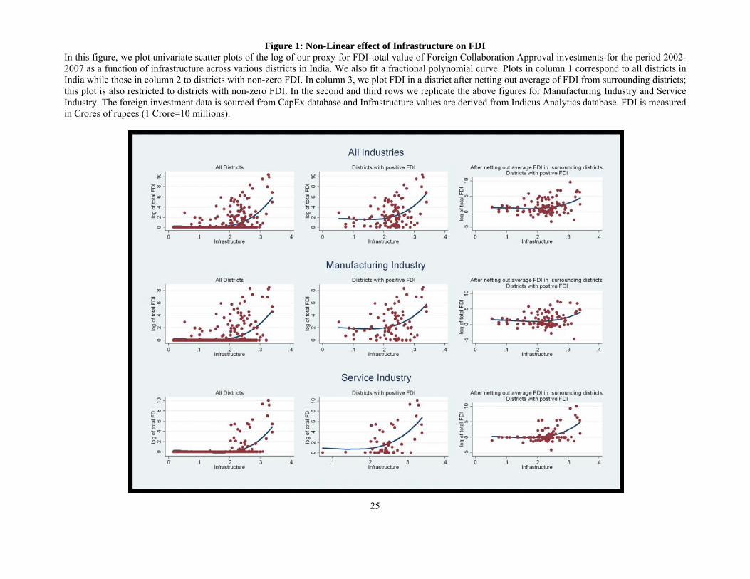
25
Figure 1: Non-Linear effect of Infrastructure on FDI
In this figure, we plot univariate scatter plots of the log of our proxy for FDI-total value of Foreign Collaboration Approval investments-for the period 2002-2007 as a function of infrastructure across various districts in India. We also fit a fractional polynomial curve. Plots in column 1 correspond to all districts in India while those in column 2 to districts with non-zero FDI. In column 3, we plot FDI in a district after netting out average of FDI from surrounding districts; this plot is also restricted to districts with non-zero FDI. In the second and third rows we replicate the above figures for Manufacturing Industry and Service Industry. The foreign investment data is sourced from CapEx database and Infrastructure values are derived from Indicus Analytics database. FDI is measured in Crores of rupees (1 Crore=10 millions).

26
Figure 2: Effect of Human Development Index, Economic Status and Crime on FDI
In this figure, we plot univariate scatter plots of the log of our proxy for FDI-total value of Foreign Collaboration Approval investments-for the period 2002- 2007 as a function of Human Development Index, Economic Status and Crime across various districts in India. We also fit a fractional polynomial curve. Plots in column 1 correspond to all districts in India while those in column 2 to districts with non-zero FDI. In column 3, we plot FDI in a district after netting out average of FDI from surrounding districts; this plot is also restricted to districts with non-zero FDI. The foreign investment data is sourced from CapEx database and Human Development Index, Economic Status and Crime values are derived from Indicus Analytics database. FDI is measured in Crores of rupees (1 Crore=10 millions).

27
Figure 3: FDI into Indian States (2002-2007)
The figure below shows the logarithm of total FDI across various states in India over the period 2002- 2007. FDI is measured in Crores of rupees (1 Crore=10 millions). The data is sourced from CapEx database.
Figure 4: Infrastructure in Indian States in 2001
The figure below shows the average Infrastructure value of the states in India for the year 2001. The Infrastructure value of district is the first major principal component obtained from the normalized Infrastructure related variables using Principal Component Analysis (PCA). The list of variables used for the PCA are: Habitations Connected by Paved Roads, Households with Electricity Connection, Households with Telephone and No. of Scheduled Commercial Bank Branches. The exact definition of these variables is given in Table 1. The data is sourced from Indicus Analytics database.

28
Figure 5: Predicted Non-linear Relationship
This figure depicts the predicted relationship obtained using the coefficients in columns 3 and 6 of Table 7. The break point is the median value of Infrastructure across all districts in India (=0.155).
-.50
.51
1.5
2
log
of to
tal v
alue
of F
DI
Afte
r net
ting
out F
DI i
n su
rrou
ndin
g di
stric
ts
0 .1 .2 .3 .4 Infrastructure
Predicted relationship using column 3 of Table 7
-.50
.51
log
of to
tal n
umbe
r of F
DI
Afte
r net
ting
out F
DI i
n su
rroun
ding
dis
trict
s
0 .1 .2 .3 .4 Infrastructure
Predicted relationship using column 6 of Table 7

29
Table 1: Variable Definitions in Indicus Database
The table below lists the variables used in our study. The indicators for each category are constructed first by normalising the variables so that each variable lies between 0 and 1. We then select the first component of the Principal Component Analysis which accounts for close to 70% of the total variance. Human Development Index (HDI) is constructed using the variables in health, empowerment and education categories. The data sourced from Indicus Analytics database is for the year 2001. Refer to the Appendix for details about the construction of the variables. Category Variable Description Infrastructure Habitations Connected
by Paved Roads
Percentage of Habitations connected by paved road. Paved road is defined as all-weather road which is motorable in all seasons of the year.
Households with Electricity Connection
Percentage of households having electricity facility out of total households.
Households with Telephone
Percentage of households having telephone connection out of total households (Only landline connections considered).
No. of Scheduled Commercial Bank Branches
Number of offices of the Scheduled Commercial Banks. Scheduled Commercial Banks in India constitute those banks which have been included in the Second Schedule of Reserve Bank of India(RBI) Act, 1934.
HDI: Education
Total Literacy Rate Literacy rate of population is defined as the percentage of literates to the total population aged 7 years and above.
Female Literacy Rate Percentage of literate females to total female population aged 7 years and above.
Male Literacy Rate Percentage of literate males to total male population aged 7 years and above.
Gender Disparity in Literacy
Gender Disparity in literacy is defined as the difference between male and female literacy rates.
Drop Out Rate (Classes I-V)
The percentage of pupils who drop out before completing Vth standard in a given school year. It does not account for the data on repeaters.
Primary to Upper-Primary Transition Index
Primary to Upper-Primary Transition Index = Enrolment in (VI-VIII) / Enrolment at (I-V) in a given time period.
Upper-Primary to Higher Grade Transition Index
Upper-Primary to Higher Grade Transition Index = Enrolment in (HS/HSS/Intermediate) / Enrolment at (VI-VIII) in a given period.
Pupil-Teacher Ratio (Primary)
Number of pupils per teacher at primary education level.

30
Category Variable DescriptionHDI: Education
Pupil-Teacher Ratio (Upper-Primary)
Number of pupils per teacher at upper-primary education level.
Education Infrastructure Index (Rural India)
Arithmetic average of the standardized variables - Safe drinking water facility, separate urinal facility and pucca building facility with equal weightings were used to construct the Index.
Education Infrastructure Index (Urban India)
Arithmetic average of the standardized variables - Safe drinking water facility, separate urinal facility and pucca building facility with equal weightings were used to construct the Index.
HDI: Health Infant Mortality Rate The number of infant deaths in less than a year of births per thousand live births.
Under 5 Mortality Rate The number of children dying before reaching fifth birthday.
Deliveries Attended by Skilled Personnel
Proportion of deliveries attended by doctor/nurse/ Auxiliary Nurse Midwife (ANM) to total deliveries either at institution or at home.
Children Fully Immunized (12-23 months)
Proportion of children, between 12 to 23 months, fully immunized against six serious but preventable diseases namely, tuberculosis, diphtheria, whooping cough (pertussis), tetanus, polio and measles.
Unmet Need For Family Planning
Proportion of currently married women in the reproductive age group who are neither having their menopause nor have had a hysterectomy nor are currently pregnant and who intent to have additional children after two years or later and is currently not using any family planning method.
Woman with greater than 3 Antenatal Care
Proportion of women who had received more than three antenatal care during pregnancy.
Use of Contraception by Modern Methods
Percentage of currently married women (age 15-44 years) using of contraception by modern methods including female sterilization, pills, IUD (Intra Uterine Device ) or condom.
Awareness Level of Women about HIV/AIDS
Percentage of Women Aware of HIV/AIDS.
Crude Birth Rate The Crude birth rate (CBR) is defined as the annual number of live births per 1,000 population.
Total Fertility Rate Total Fertility Rate (TFR) indicates the average number of children expected to be born per woman.

31
Category Variable Description HDI: Health Weight for Age
(percentage children (0-59 months) with weight lower than -2SD for their given age
Weight-for-age is a composite index of height-for-age and weight-for-height. It takes into account both acute and chronic malnutrition. Children whose weight-for-age is below minus two standard deviations from the median of the reference population are classified as underweight.
Households using adequate Iodized Salt
Iodine is an important micronutrient. Adequately iodised (above 15 parts per million), Inadequately iodised (below 15 ppm).
HDI: Empowerment
Crime Against Women Number of crime against women as percentage to total crime. Crime against women includes rape, kidnapping, dowry deaths, molestation, sexual harassment, cruelty by husband and relatives and importation of girls.
Under-aged Girl Marriage
Percentage of girls who were below the legal age at marriage (18 yrs) at the time of their marriage.
Birth Order of 3 and Above
Percentage of the third and higher order births during three years preceding the survey.
Sex Ratio Number of females per thousand males. Female Work
Participation Rate The percentage of total female workers (main and marginal) to total female population. Main workers are workers who had worked for the major part of the reference period (i.e. 6 months or more). Marginal workers are workers who had not worked for the major part of the reference period (i.e. less than 6 months).
Economic Status
Work Participation Rate Work Participation Rate (WPR) is defined as percentage of total workers (main+marginal) to the total population. Main workers are those who had worked for the major part of the reference period (i.e. 6 months or more). Marginal workers are workers who had not worked for the major part of the reference period (i.e. less than 6 months).
Demographics Total Population Number of total persons. Crime Violent Crimes Proportion of Violent crimes as percentage of total
number of crimes. Violent crimes include murder, attempt to commit murder, culpable homicide not amounting to murder, rape, kidnapping and abduction, dacoity, robbery, riots, arson and dowry death.
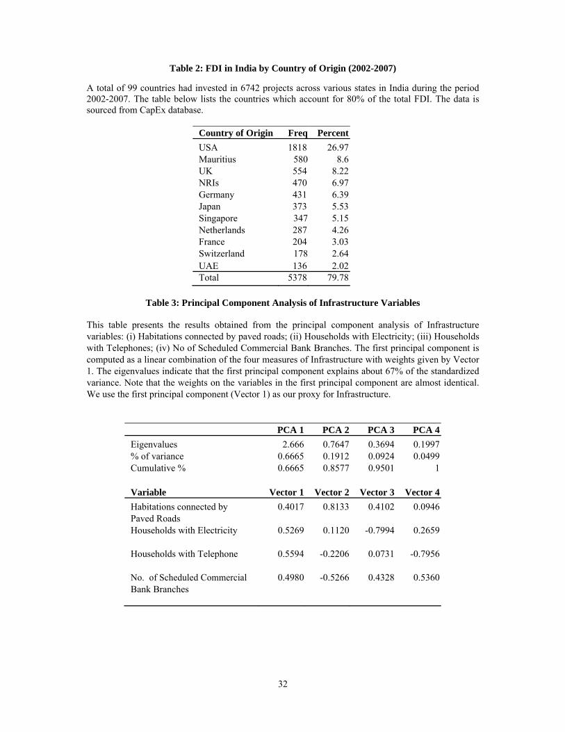
32
Table 2: FDI in India by Country of Origin (2002-2007)
A total of 99 countries had invested in 6742 projects across various states in India during the period 2002-2007. The table below lists the countries which account for 80% of the total FDI. The data is sourced from CapEx database.
Country of Origin Freq PercentUSA 1818 26.97Mauritius 580 8.6UK 554 8.22NRIs 470 6.97Germany 431 6.39Japan 373 5.53Singapore 347 5.15Netherlands 287 4.26France 204 3.03Switzerland 178 2.64UAE 136 2.02Total 5378 79.78
Table 3: Principal Component Analysis of Infrastructure Variables
This table presents the results obtained from the principal component analysis of Infrastructure variables: (i) Habitations connected by paved roads; (ii) Households with Electricity; (iii) Households with Telephones; (iv) No of Scheduled Commercial Bank Branches. The first principal component is computed as a linear combination of the four measures of Infrastructure with weights given by Vector 1. The eigenvalues indicate that the first principal component explains about 67% of the standardized variance. Note that the weights on the variables in the first principal component are almost identical. We use the first principal component (Vector 1) as our proxy for Infrastructure.
PCA 1 PCA 2 PCA 3 PCA 4 Eigenvalues 2.666 0.7647 0.3694 0.1997 % of variance 0.6665 0.1912 0.0924 0.0499 Cumulative % 0.6665 0.8577 0.9501 1
Variable Vector 1 Vector 2 Vector 3 Vector 4 Habitations connected by 0.4017 0.8133 0.4102 0.0946 Paved Roads Households with Electricity 0.5269 0.1120 -0.7994 0.2659
Households with Telephone 0.5594 -0.2206 0.0731 -0.7956
No. of Scheduled Commercial 0.4980 -0.5266 0.4328 0.5360 Bank Branches

33
Table 4: Descriptive Statistics
In this table, we present the summary statistics of variables used in the regressions. Panel A presents summary statistics for Foreign Direct Investments (FDI) across various districts in India over the period 2002-2007. Panel A1 shows the value of FDI while Panel A2 shows the number of FDI projects. Panel B presents summary statistics of the independent variables for the year 2001. The details for construction of these variables are provided in Table 1. The source of Panel A1 and A2 is CapEx database and that of Panel B is Indicus Analytics database. The unit of sample is district and the unit of measurement of the variable is described in parenthesis.
Panel A1: Value of FDI (2002-2007)
Obs Mean Std.Dev Min Max 1st Quartile Median 3rd Quartile Districts with positive investment
All Industries (in Crores*) 563 141.131 1658.598 0 30632.89 0 0 0 105Manufacturing Industry (in Crores) 563 35.653 319.934 0 4619.71 0 0 0 81Service Industry (in Crores) 563 84.107 1163.218 0 23330.82 0 0 0 51
Panel A2: Number of FDI projects (2002-2007)
All Industries 563 8.092 71.189 0 1218 0 0 1 105Manufacturing Industry 563 3.611 27.48 0 476 0 0 0 81Service Industry 563 4.161 41.2754 0 684 0 0 0 51
Panel B: Independent Variables
HDI 563 0.101 0.029 0.045 0.177 0.076 0.099 0.121Infrastructure 563 0.161 0.071 0.016 0.339 0.105 0.155 0.221Economic Status 563 0.464 0.127 0.159 0.877 0.366 0.468 0.554Crime 563 0.287 0.158 0 1 0.164 0.236 0.389GDP per capita (in '000) 563 17.54 10.48 4 90 11 15 21log of population (in '000) 563 7.144 0.957 3.503 9.17 6.767 7.315 7.804Dummy for Metro 563 0.039 0.193 0 1 0 0 0
* 1 Crore = 10 milllions

34
Table 5: Correlation Matrix for Variables employed in the Multivariate Analysis
This table shows the pair wise correlations among the variables used in our multivariate analysis. The variables in rows 1-3 correspond to the dependent variables while the others are the explanatory variables in our regressions. The FDI variables are measured from 2002-2007 while the other variables are measured in 2001.
(1) (2) (3) (4) (5) (6) (7) (8) (9) (10)
(1) 1log of total value of FDI (for All Industries) log of total value of FDI (2) 0.9497 1 (for Manufacturing Industry) log of total value of FDI (3) 0.7855 0.653 1 (for Service Industry) HDI (4) 0.3001 0.2635 0.2396 1
Infrastructure (5) 0.3879 0.3508 0.3134 0.7819 1
Economic Status (6) -0.0543 -0.0512 -0.0795 0.1614 0.1559 1
Crime (7) -0.2379 -0.2135 -0.1595 -0.4784 -0.5529 -0.3063 1
GDP per Capita (8) 0.5187 0.4939 0.4676 0.5866 0.6918 0.054 -0.3992 1
log of population (9) 0.2541 0.2246 0.1992 0.0277 0.075 -0.3875 -0.1591 -0.0536 1
Dummy for Metro (10) 0.5232 0.4879 0.5466 0.1971 0.2493 -0.1192 -0.1399 0.3258 0.224 1

35
Table 6: District-level cross-sectional regressions with state fixed effects
This table reports results from district-level cross-sectional regressions. The dependent variable equals the logarithm of total value of FDI in a district in columns 1-3 and the logarithm of number of FDI projects in a district in columns 4-6. FDI is measured over the time period 2002-2007 while the independent variables are measured in 2001. The FDI data is sourced from CapEx database while all other variables are from Indicus Analytics. Robust standard errors clustered by state are reported in parentheses. *** ** and * denote statistical significance at 1%, 5% and 10% respectively. Columns 1 and 4, 2 and 5 and 3 and 6 run the following regression specification: → ,∑ ` = + ∗ → ,` + ∗ → ,` + → ,∑ ` = + ∗ → ,` + ∗ → ,` + ∗ → ,` + → ,∑ ` = + ∗ → ,` ∗ ( → ,` + ℎ → ,` ) + ∗ → ,` +
Dependent Variable is : log of Value of FDI log of No. of FDI projects (1) (2) (3) (4) (5) (6)
Infrastructure 2.283 -19.053*** 0.866 -11.360*** (1.952) (5.437) (1.359) (3.257)
Infrastructure square 71.064*** 40.722*** (18.498) (10.580)
Infrastructure*(districts ranking as -2.958* -1.257 low Infrastructure within the country):β1 (1.540) (1.252) Infrastructure*(districts ranking as 12.705*** 8.300***high Infrastructure within the country):β2 (4.359) (2.444) Districts ranking as high -2.704*** -1.824***Infrastructure within the country (0.867) (0.392) HDI -7.621* -8.175 -8.423* -3.921 -4.238 -4.568
(4.436) (5.043) (4.661) (2.893) (3.396) (3.117) Crime 0.618* 0.507* 0.533 0.513** 0.450* 0.474*
(0.313) (0.278) (0.317) (0.225) (0.233) (0.245) Economic Status -0.139 -0.146 -0.108 0.283 0.278 0.277
(0.531) (0.529) (0.535) (0.322) (0.331) (0.324) GDP per capita 0.065*** 0.053*** 0.057*** 0.059*** 0.052*** 0.054***
(0.018) (0.016) (0.016) (0.010) (0.008) (0.009) log of population 0.360** 0.350** 0.355** 0.414*** 0.409*** 0.412***
(0.147) (0.146) (0.143) (0.102) (0.106) (0.102) Dummy for Metro 2.433*** 2.041** 2.150** 1.423*** 1.198** 1.227**
(0.802) (0.785) (0.818) (0.462) (0.453) (0.466) Dummy for districts adjacent to 0.169 0.168 0.184 0.161 0.160 0.171 district with Metro city (0.138) (0.152) (0.154) (0.103) (0.107) (0.109) State fixed effects YES YES YES YES YES YES Observations 563 563 563 563 563 563 P value of β1-β2
× × 0.002 × × 0.001 Adj R-squared 0.457 0.488 0.476 0.623 0.645 0.643

36
Table 7: District-level cross-sectional regressions with state fixed effects after netting out average FDI in the surrounding districts
This table reports results from district-level cross-sectional regressions. The dependent variable equals the logarithm of total value of FDI in a district minus the average total value of FDI in its surrounding districts in columns 1-3 and the logarithm of Number of FDI projects in a district minus the average Number of FDI projects in its surrounding districts in columns 4-6 FDI is measured over the time period 2002-2007 while the independent variables are measured in 2001. The FDI data is sourced from CapEx database while all other variables are from Indicus Analytics. Robust standard errors clustered by state are reported in parentheses. *** ** and * denote statistical significance at 1%, 5% and 10% respectively. Columns 1 and 4, 2 and 5 and 3 and 6 run the following regression specification: ( → ,∑ ` ) − ( → ,∑ ` ) = + ∗ → ,` + ∗ → ,` + ( → ,∑ ` ) − ( → ,∑ ` ) = + ∗ → ,` + ∗ → ,` + ∗ → ,` + ( → ,∑ ` ) − ( → ,∑ ` ) = + ∗ → ,` ∗ → ,` + ℎ → ,` + ∗ → ,` +
Dependent Variable is : log of Value of FDI- log of No. of FDI projects - log of avg Value of FDI log of avg No. of FDI projects in surrounding districts in surrounding districts (1) (2) (3) (4) (5) (6)
Infrastructure 3.741 -16.960*** 1.358 -11.043*** (2.361) (5.113) (1.196) (3.198) Infrastructure square 68.948*** 41.305*** (15.550) (9.228) Infrastructure*(districts ranking as -2.871 -1.968 low Infrastructure within the country):β1 (2.071) (1.204) Infrastructure*(districts ranking as 13.451*** 8.047*** high Infrastructure within the country):β2 (3.917) (1.962) Districts ranking as high -2.632*** -1.733*** Infrastructure within the country (0.838) (0.377) HDI -11.203** -11.741** -11.871** -5.066* -5.388* -5.582* (4.325) (4.859) (4.623) (2.518) (2.875) (2.752) Crime 0.230 0.122 0.128 0.162 0.097 0.108 (0.277) (0.275) (0.301) (0.191) (0.213) (0.225) Economic Status -0.071 -0.078 -0.012 0.240 0.236 0.260 (0.428) (0.449) (0.446) (0.258) (0.285) (0.278) GDP per Capita 0.050*** 0.038*** 0.042*** 0.043*** 0.036*** 0.038*** (0.010) (0.009) (0.010) (0.005) (0.004) (0.005) log of population 0.249** 0.239** 0.244** 0.361*** 0.355*** 0.358*** (0.097) (0.099) (0.095) (0.081) (0.086) (0.082) Dummy for Metro 2.240*** 1.860** 1.970** 1.377*** 1.150** 1.196** (0.785) (0.762) (0.778) (0.469) (0.466) (0.472) Dummy for districts adjacent to -0.575*** -0.576*** -0.561*** -0.337*** -0.338*** -0.327***district with Metro city (0.194) (0.198) (0.192) (0.121) (0.119) (0.116) State fixed effects YES YES YES YES YES YES Observations 563 563 563 563 563 563 P value of β1-β2 × × 0.001 × × 0.000 Adj R-squared 0.265 0.294 0.284 0.419 0.446 0.439

37
Table 8: Robustness tests using FDI in a district minus maximum FDI into surrounding districts as the dependent variable
This table reports results from district-level cross-sectional regressions. The dependent variable equals the logarithm of total value of FDI in a district after netting out maximum of FDI in surrounding districts in columns 1-3 and logarithm of Number of FDI projects in a district after netting out maximum of Number of FDI projects in surrounding districts in columns 4-6. FDI is measured over the time period 2002-2007 while the independent variables are measured in 2001. The FDI data is sourced from CapEx database while all other variables are from Indicus Analytics. Robust standard errors clustered by state are reported in parentheses. *** ** and * denote statistical significance at 1%, 5% and 10% respectively. Columns 1 and 4, 2 and 5 and 3 and 6 run the following regression specification: → ,∑(` ) − → ,∑ ` = + ∗ → ,` + ∗ → ,` + → ,∑(` ) − → ,∑ ` = + ∗ → ,` + ∗ → ,` + ∗ → ,` + → ,∑(` ) − → ,∑ ` = + ∗ → ,` ∗ → ,` + ℎ → ,` + ∗ → ,` +
Dependent Variable is : log of Value of FDI- log of No. of FDI projects - log of max Value of FDI log of max No. of FDI projects in surrounding districts in surrounding districts (1) (2) (3) (4) (5) (6)
Infrastructure 3.601 -16.361** 1.338 -14.899*** (3.458) (7.401) (2.477) (4.839)
Infrastructure square 66.488*** 54.082*** (19.994) (14.444)
Infrastructure*(districts ranking as -3.290 -3.195 low Infrastructure within the country): β1 (3.744) (1.897) Infrastructure*(districts ranking as 10.226* 8.249** high Infrastructure within the country): β2 (5.275) (3.554) Districts ranking as high -1.949* -1.862*** Infrastructure within the country (1.126) (0.603) HDI -20.768** -21.287** -21.112*** -9.764* -10.185* -10.246*
(7.534) (7.686) (7.586) (5.493) (5.243) (5.310) Crime -0.365 -0.469 -0.465 -0.498 -0.582 -0.568
(0.639) (0.671) (0.658) (0.382) (0.415) (0.414) Economic Status -1.365 -1.372 -1.285 -0.292 -0.298 -0.254
(1.021) (0.999) (1.035) (0.637) (0.627) (0.649) GDP per capita 0.047*** 0.036*** 0.041*** 0.036*** 0.027*** 0.031***
(0.012) (0.013) (0.012) (0.008) (0.009) (0.008) log of population -0.170 -0.179 -0.175 0.126 0.118 0.122
(0.167) (0.167) (0.168) (0.123) (0.127) (0.126) Dummy for Metro 1.901** 1.534* 1.708* 1.372** 1.074* 1.181**
(0.841) (0.833) (0.852) (0.516) (0.525) (0.531) Dummy for districts adjacent to -2.002*** -2.002*** -1.991*** -1.361*** -1.362*** -1.351*** district with Metro city (0.528) (0.527) (0.522) (0.335) (0.326) (0.325) State fixed effects YES YES YES YES YES YESObservations 563 563 563 563 563 563 P value of β1- β2 × × 0.042 × × 0.005 Adj R 0.277 0.288 0.281 0.345 0.367 0.356

38
Table 9: Test exploiting inter-industry differences in the role of public infrastructure in attracting FDI This table reports results from district-level cross-sectional regressions. The dependent variable equals the logarithm of total value of FDI in a district in columns 1-2 and the logarithm of Number of FDI projects in a district in columns 3-4. FDI is measured over the time period 2002-2007 while the independent variables are measured in 2001. FDI Propensity is measured as the ratio of FDI in a sector to total FDI in India for the year 2001. The FDI data is sourced from CapEx database while all other variables are from Indicus Analytics. The robust standard errors reported in parentheses are clustered by state. *** ** and * denote statistical significance at 1%, 5% and 10% respectively. Columns 1 and 3 and 2 and 4 run the following regression specification: ,∑(` ) = + + ,` + ,` ∗ _ , +
,∑(` ) = + [ + `, + ℎ ,` ∗ ,` ] ∗ _ , +
Dependent Variable is : log of Value of FDI log of No. of FDI projects
(1) (2) (3) (4)
Infrastructure*FDI Propensity -22.327** -23.070***
(8.292) (7.985)
Infrastructure square*FDI Propensity 96.979*** 95.507***
(29.043) (26.594)
Infrastructure*(districts ranking as low Infrastructure 7.380* 8.230**
within country)*FDI Propensity (3.637) (3.502)
Infrastructure*(districts ranking as high Infrastructure 8.638*** 8.106***
within country)* FDI Propensity (2.337) (2.103)
FDI Propensity 1.162** -0.747* 1.229** -0.840*
(0.522) (0.421) (0.520) (0.414)
District fixed effects YES YES YES YES Observations 3378 3378 3378 3378
Adj R2 0.475 0.449 0.526 0.468

39
Table 10: Robustness - Effect of Infrastructure on FDI year-by-year
This table reports results from district-level cross-sectional regressions. The dependent variable equals the logarithm of total value of FDI in a district in columns 1-5 and the logarithm of Number of FDI projects in a district in columns 5-10. FDI is measured for each individual year mentioned in the column (from 2007 to 2003).Independent variables are measured in 2001 except for log of FDI in surrounding districts and log of domestic investment which are lagged by an year with respect to the dependent variable . The FDI data is sourced from CapEx database while all other variables are from Indicus Analytics. Robust standard errors clustered by state are reported in parentheses. *** ** and * denote statistical significance at 1%, 5% and 10% respectively. Columns 1 -10 run the following regression specification: → , = + ∗ → ,` ∗ → ,` + ℎ → ,` + ∗ → ,` +
Dependent Variable is : log (Value of FDIt) log (No. of FDI projectst) 2007 2006 2005 2004 2003 2007 2006 2005 2004 2003 (1) (2) (3) (4) (5) (6) (7) (8) (9) (10)
Infrastructure*(districts ranking as -0.567 -0.950 -1.140 -0.127 -0.642 -0.936 -1.441** -1.137** -1.234** -0.840 low Infrastructure within the country):β1 (1.231) (1.146) (0.999) (1.153) (0.632) (0.579) (0.632) (0.477) (0.548) (0.735) Infrastructure*(districts ranking as 6.544* 7.232*** 5.884** 13.753*** 11.967*** 2.129** 0.923* 2.772** 6.073*** 8.470*** high Infrastructure within the country): β2 (3.683) (2.496) (2.505) (2.868) (2.455) (0.984) (0.508) (1.206) (1.442) (1.744) Districts ranking as high -1.429* -1.692*** -1.418*** -2.723*** -2.370*** -0.658*** -0.532** -0.782*** -1.394*** -1.673*** Infrastructure within the country (0.699) (0.468) (0.409) (0.499) (0.386) (0.171) (0.206) (0.249) (0.255) (0.295) HDI -5.929** -4.537** -5.242** -8.838*** -6.549** -3.136 -0.971 -4.180** -5.457** -5.108**
(2.757) (1.708) (2.397) (3.186) (2.700) (2.068) (1.454) (1.660) (2.004) (2.116) Crime 0.259 0.264 0.070 0.177 0.548** 0.150 0.195* 0.224* 0.211 0.507***
(0.173) (0.259) (0.192) (0.265) (0.220) (0.125) (0.097) (0.109) (0.151) (0.154) Economic Status -0.347 -0.028 -0.120 0.160 -0.461 0.126 -0.029 -0.027 0.033 0.042
(0.409) (0.323) (0.366) (0.413) (0.452) (0.207) (0.152) (0.206) (0.235) (0.280) GDP per capita 0.033** 0.033** 0.028* 0.031** 0.031*** 0.030*** 0.018*** 0.022*** 0.025*** 0.022**
(0.014) (0.016) (0.014) (0.014) (0.010) (0.004) (0.005) (0.005) (0.006) (0.009) log of population 0.077 0.096 0.099 0.118 0.070 0.091** 0.078** 0.096** 0.073 0.086
(0.074) (0.080) (0.065) (0.083) (0.080) (0.041) (0.031) (0.037) (0.043) (0.051) Dummy for Metro 1.408*** 1.289** 1.295** 1.731** 0.671 0.459* 0.566*** 0.633*** 1.019** 0.942**
(0.494) (0.577) (0.492) (0.647) (0.459) (0.230) (0.198) (0.186) (0.384) (0.406) Dummy for districts adjacent to -0.070 -0.037 0.003 0.082 -0.006 -0.049* -0.064*** -0.050* -0.019 -0.028 district with Metro city (0.081) (0.057) (0.072) (0.097) (0.057) (0.028) (0.021) (0.029) (0.064) (0.062) log (FDI in surrounding districtst-1) 0.035 0.000 0.009 0.039 0.052*** 0.042 0.020 0.047*** 0.039** 0.042* (0.074) (0.036) (0.013) (0.038) (0.017) (0.043) (0.023) (0.010) (0.018) (0.023) log (domestic investmentt-1) -0.022* -0.012* 0.006 0.019 0.026 0.034 0.038 0.076** 0.165*** 0.222*** (0.011) (0.006) (0.010) (0.012) (0.020) (0.024) (0.024) (0.028) (0.043) (0.057) State fixed effects YES YES YES YES YES YES YES YES YES YES Observations 563 563 563 563 563 563 563 563 563 563 Adj R-squared 0.377 0.399 0.378 0.470 0.422 0.541 0.453 0.525 0.605 0.606

40
Table 11: Robustness tests controlling for domestic private investment into the district This table reports results from district-level cross-sectional regressions. The dependent variable equals the logarithm of total value of FDI in a district minus the average value of FDI in its surrounding districts in columns 1-2 and the logarithm of Number of FDI projects in a district minus the average Number of FDI projects in its surrounding districts in columns 3-4. FDI is measured over the time period 2002-2007 while the independent variables are measured in 2001. The FDI data is sourced from CapEx database while all other variables are from Indicus Analytics. Robust standard errors clustered by state are reported in parentheses. *** ** and * denote statistical significance at 1%, 5% and 10% respectively. Columns 1 and 3 and 2 and 4 run the following regression specification: ( → ,∑ ` ) − ( → ,∑ ` ) = + ∗ → ,` + ∗ → ,` + ∗ → ,` + ( → ,∑ ` ) − ( → ,∑ ` ) = + ∗ → ,` ∗ ( → ,` + ℎ → ,` ) + ∗ → ,` +
Dependent Variable is : log of Value of FDI- log of No. of FDI projects - log of avg Value of FDI log of avg No. of FDI projects in surrounding districts in surrounding districts (1) (2) (3) (4) Infrastructure -17.476*** -11.559*** (5.099) (3.246) Infrastructure square 70.324*** 42.679*** (15.488) (9.296) Infrastructure*(districts ranking as -3.096 -2.213* low Infrastructure within the country): β1 (2.108) (1.216) Infrastructure*(districts ranking as 13.500*** 8.100*** high Infrastructure within the country): β2 (3.881) (1.956) Districts ranking as high -2.670*** -1.776*** Infrastructure within the country (0.832) (0.380) log of Domestic Investment 0.015 0.012 0.015* 0.013 in all Industries (0.014) (0.014) (0.008) (0.008) HDI -11.632** -11.781** -5.278* -5.485* (4.875) (4.636) (2.901) (2.774) Crime 0.130 0.134 0.105 0.115 (0.283) (0.308) (0.223) (0.234) Economic Status -0.030 0.027 0.283 0.302 (0.444) (0.442) (0.297) (0.291) GDP per Capita 0.036*** 0.040*** 0.035*** 0.037*** (0.009) (0.010) (0.004) (0.005) log of population 0.204* 0.216* 0.320*** 0.328*** (0.112) (0.111) (0.082) (0.080) Dummy for Metro 1.865** 1.976** 1.155** 1.202** (0.763) (0.781) (0.465) (0.472) Dummy for Districts adjacent to -0.570*** -0.556*** -0.332*** -0.322*** districts with Metro city (0.198) (0.192) (0.119) (0.115) State fixed effects YES YES YES YES Observations 563 563 563 563 Adj R-squared 0.294 0.283 0.447 0.440

41
Table 12: Robustness tests controlling for possible lobbying for FDI This table reports results from district-level cross-sectional regressions. The dependent variable equals the logarithm of total value of FDI in a district minus the average value of FDI in its surrounding districts in columns 4-6. The sample in columns 1 and 2 (3 and 4) is restricted to investments above (below) the median value FDIs in India. In columns 5 and 6 we exclude districts where special Economic Zones are located. FDI is measured over the time period 2002-2007 while the independent variables are measured in 2001. The FDI data is sourced from CapEx database while all other variables are from Indicus Analytics. Robust standard errors clustered by state are reported in parentheses. ***, ** and * denote statistical significance at 1%, 5% and 10% respectively. Columns 1, 3 and 5 and 2,4 and 6 run the following regression specification: ( → ,∑ ` ) − ( → ,∑ ` ) = + ∗ → ,` + ∗ → ,` + ∗ → ,` + ( → ,∑ ` ) − ( → ,∑ ` ) = + ∗ → ,` ∗ ( → ,` + ℎ → ,` ) + ∗ → ,` +
Dependent Variable is : log of Value of FDI- log of Value of FDI- log of Value of FDI- log of avg Value of FDI log of avg Value of FDI log of avg Value of FDI in surrounding districts in surrounding districts in surrounding districts (1) (2) (3) (4) (5) (6)
Infrastructure -13.433* -3.973 -14.366*** (6.603) (2.820) (4.819)
Infrastructure square 64.709*** 19.790** 58.658*** (21.098) (7.952) (16.519)
Infrastructure*(districts ranking as -0.763 1.287 -3.145 low Infrastructure within country):β1 (3.311) (1.721) (2.384) Infrastructure*(districts ranking as 13.915** 4.320* 10.523** high Infrastructure within country): β2 (6.311) (2.188) (4.503) Districts ranking as high Infrastructure -2.238* -0.584 -2.119** within country (1.152) (0.344) (0.839) HDI -25.784** -25.652** -2.923 -2.932 -12.319** -11.693**
(10.043) (10.197) (3.296) (3.300) (5.135) (4.845) Crime -0.581 -0.580 -0.447* -0.433* 0.018 0.008
(0.682) (0.680) (0.029) (0.230) (0.322) (0.333) Economic Status -1.291 -0.217 0.381 0.379 -0.372 -0.340
(1.025) (1.042) (0.356) (0.349) (0.505) (0.506) GDP per Capita 0.029** 0.033** -0.004 -0.003 0.030** 0.031**
(0.013) (0.013) (0.005) (0.005) (0.011) (0.012) log of population -0.092 -0.088 0.080 0.081 0.184* 0.190**
(0.195) (0.195) (0.059) (0.060) (0.093) (0.089) Dummy for Metro 2.123** 2.258** 0.851*** 0.901*** 2.683** 2.764**
(0.947) (0.959) (0.268) (0.284) (0.981) (1.016) State fixed effects YES YES YES YES YES YES Observations 549 549 549 549 549 549 Adj R2 0.181 0.175 0.181 0.172 0.211 0.204

42
Table 13: Role of public infrastructure in attracting FDI into manufacturing industries
This table reports results from district-level cross-sectional regressions. The dependent variable equals the logarithm of total value of FDI in a district minus the average value of FDI in its surrounding districts in columns 1-2 and the logarithm of Number of FDI projects in a district minus the average Number of FDI projects in its surrounding districts in columns 3-4 for service industries. FDI is measured over the time period 2002-2007 while the independent variables are measured in 2001. The FDI data is sourced from CapEx database while all other variables are from Indicus Analytics. Robust standard errors clustered by state are reported in parentheses. *** ** and * denote statistical significance at 1%, 5% and 10% respectively. Columns 1 and 3 and 2 and 4 run the following regression specification: ( → ,∑ ` ) − ( → ,∑ ` ) = + ∗ → ,` + ∗ → ,` + ∗ → ,` + ( → ,∑ ` ) − ( → ,∑ ` ) = + ∗ → ,` ∗ ( → ,` + ℎ → ,` ) + ∗ → ,` +
Dependent Variable is : log of Value of FDI- log of No. of FDI projects - log of avg Value of FDI log of avg No. of FDI projects in surrounding districts in surrounding districts (1) (2) (3) (4)
Infrastructure -14.821*** -9.967*** (4.121) (3.004)
Infrastructure square 58.313*** 34.993*** (13.457) (9.189)
Infrastructure*(districts ranking as -2.454 -1.556 low Infrastructure within the country):β1 (2.075) (1.025) Infrastructure*(districts ranking as 10.296*** 6.546*** high Infrastructure within the country): β2 (3.656) (1.938) Districts ranking as high -2.057** -1.497*** Infrastructure within the country (0.761) (0.355) log of Domestic Investment 0.017 0.014 0.010 0.009 in Manufacturing Industry (0.015) (0.015) (0.009) (0.009) HDI -11.308** -11.409*** -5.981** -6.234**
(4.161) (3.901) (2.540) (2.395) Crime 0.155 0.165 0.217 0.233
(0.254) (0.273) (0.198) (0.206) Economic Status 0.089 0.136 0.315 0.318
(0.424) (0.423) (0.283) (0.265) GDP per Capita 0.035*** 0.039*** 0.036*** 0.037***
(0.010) (0.011) (0.003) (0.003) log of population 0.146 0.156* 0.294*** 0.300***
(0.091) (0.088) (0.072) (0.068) Dummy for Metro 1.540** 1.648** 0.906** 0.937**
(0.737) (0.741) (0.423) (0.424) Dummy for Districts adjacent to -0.404* -0.394* -0.228** -0.220** district with Metro city (0.233) (0.227) (0.105) (0.104) State fixed effects YES YES YES YES Observations 563 563 563 563 Adj R-squared 0.237 0.225 0.423 0.418

43
Table 14: Role of public infrastructure in attracting FDI into service industries
This table reports results from district-level cross-sectional regressions. The dependent variable equals the logarithm of total value of FDI in a district minus the average value of FDI in its surrounding districts in columns 1-2 and the logarithm of Number of FDI projects in a district minus the average Number of FDI projects in its surrounding districts in columns 3-4 for service industries. FDI is measured over the time period 2002-2007 while the independent variables are measured in 2001. The FDI data is sourced from CapEx database while all other variables are from Indicus Analytics. Robust standard errors clustered by state are reported in parentheses. *** ** and * denote statistical significance at 1%, 5% and 10% respectively. Columns 1 and 3 and 2 and 4 run the following regression specification: ( → ,∑ ` ) − ( → ,∑ ` ) = + ∗ → ,` + ∗ → ,` + ∗ → ,` + ( → ,∑ ` ) − ( → ,∑ ` ) = + ∗ → ,` ∗ ( → ,` + ℎ → ,` ) + ∗ → ,` +
Dependent Variable is : log of Value of FDI- log of No. of FDI projects - log of avg Value of FDI log of avg No. of FDI projects in surrounding districts in surrounding districts (1) (2) (3) (4) Infrastructure -18.864*** -12.301*** (6.029) (2.857) Infrastructure square 71.243*** 48.391*** (19.068) (8.736) Infrastructure*(districts ranking as -0.601 -0.840 low Infrastructure within the country): β1 (1.093) (0.783) Infrastructure*(districts ranking as 12.558*** 9.033*** high Infrastructure within the country): β2 (3.332) (1.915) Districts ranking as high -2.479*** -1.743*** Infrastructure within the country (0.691) (0.310) log of Domestic Investment -0.028 -0.034 0.006 0.003 in Service Industry (0.022) (0.024) (0.011) (0.012) HDI -7.484** -7.672** -6.120** -6.221** (3.248) (2.800) (2.563) (2.386) Crime 0.121 0.180 0.114 0.141 (0.205) (0.214) (0.141) (0.146) Economic Status -0.267 -0.280 0.063 0.073 (0.457) (0.463) (0.291) (0.283) GDP per Capita 0.022*** 0.027*** 0.016* 0.019** (0.006) (0.008) (0.008) (0.009) log of population 0.098 0.111 0.089 0.096* (0.094) (0.100) (0.055) (0.055) Dummy for Metro 1.771*** 1.913*** 1.220*** 1.311*** (0.639) (0.686) (0.432) (0.460) Dummy for Districts adjacent to -0.462*** -0.445*** -0.332*** -0.321*** district with Metro city (0.137) (0.131) (0.084) (0.079) State fixed effects YES YES YES YES Observations 563 563 563 563 Adj R-squared 0.374 0.346 0.434 0.408

44
Appendix
Description of the “Indian Development Landscape” database
The “Indian Development Landscape” in the Indicus database provides information
pertaining to Agriculture, Demography, Economic Status, Education, Empowerment, Health and
Infrastructure. Specifically, the variables in the categories include:
• Agriculture (A)- total cultivators, total agricultural labours, area sown more than once, net area
sown, net irrigated area.
• Demography (D) - population (total, male and female, urban and rural), households (total, urban
and rural), population density, migration, population of scheduled castes and scheduled tribes.
• Economic Status (Ec) - head count ratio, marginal workers as a percentage of total population,
work participation rate.
• Education (Ed) - literacy rates, gender gaps in literacy, percentage transiting from primary to
upper-primary school level, percentage transiting from upper-primary to high school level, pupil-
teacher ratio at the primary level, pupil-teacher ratio at the upper-primary level.
• Empowerment (M) - crimes committed against women, girls married below legal age, sex ratio,
female work participation rate.
• Environment (N) - wasteland areas, area affected by drought, area affected by flood.
• Health (H) - infant mortality, deliveries attended by skilled personnel, immunization, ante-natal
care, unmet need for family planning, adoption of modern methods of contraception, awareness
about HIV/AIDS.
• Crime (C) – number of armed robberies, murders, kidnappings, etc.
• Infrastructure (I) - percentage of habitations connected by paved roads, percentage of households
with electricity, percentage of households with telephone, number of scheduled commercial bank
branches.
The sources of the above variables are shown in the Table below:

45
Source: Indicus Analytics