Infrared thermography 230 pages ebook – electrical and industrial applications

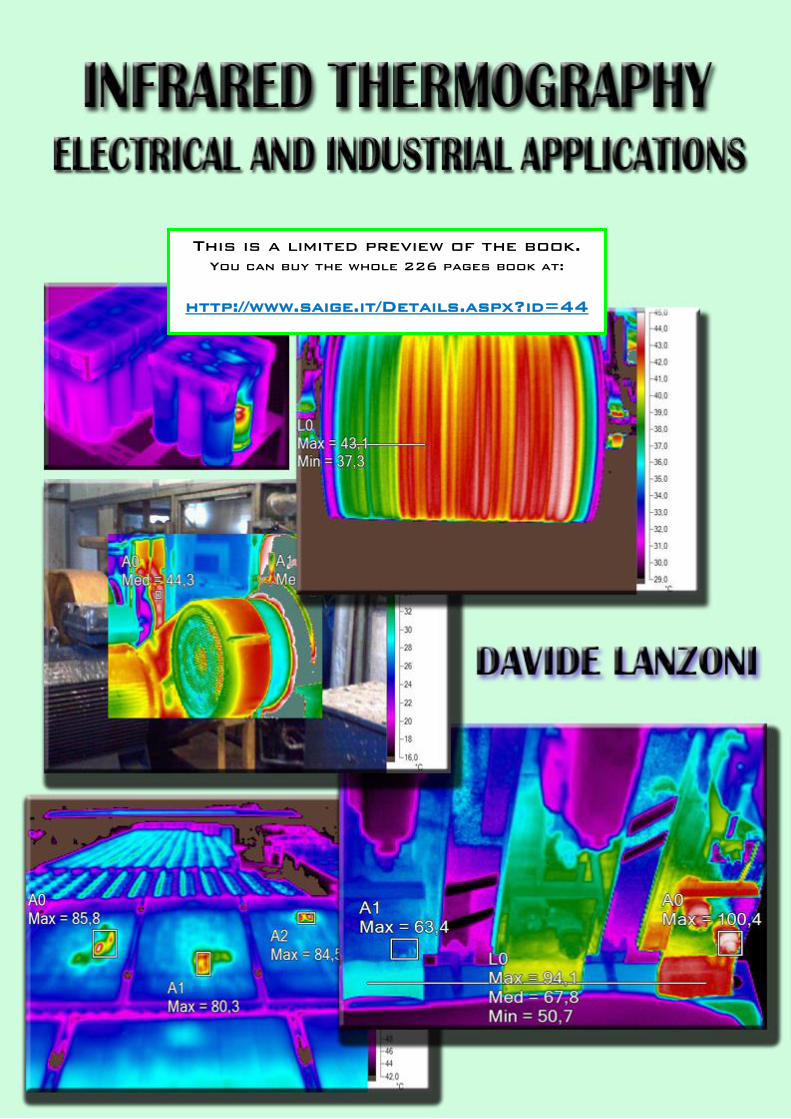
This is a limited preview of the book.

You can buy the whole 226 pages book at:

http://www.saige.it/Details.aspx?id=44

1

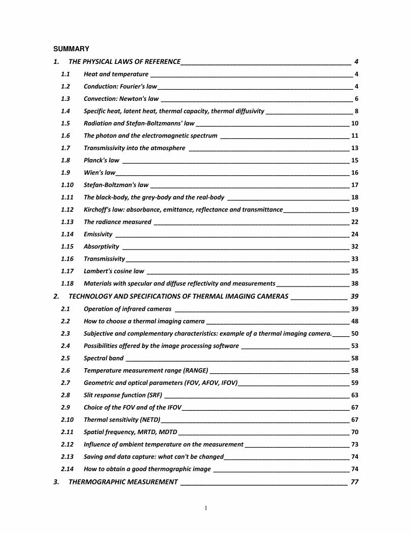
SUMMARY

1. THE PHYSICAL LAWS OF REFERENCE _____________________________________________ 4

1.1 Heat and temperature __________________________________________________________ 4

1.2 Conduction: Fourier's law ________________________________________________________ 4

1.3 Convection: Newton's law _______________________________________________________ 6

1.4 Specific heat, latent heat, thermal capacity, thermal diffusivity _________________________ 8

1.5 Radiation and Stefan-Boltzmanns' law ____________________________________________ 10

1.6 The photon and the electromagnetic spectrum _____________________________________ 11

1.7 Transmissivity into the atmosphere ______________________________________________ 13

1.8 Planck's law _________________________________________________________________ 15

1.9 Wien's law___________________________________________________________________ 16

1.10 Stefan-Boltzman's law _________________________________________________________ 17

1.11 The black-body, the grey-body and the real-body ___________________________________ 18

1.12 Kirchoff's law: absorbance, emittance, reflectance and transmittance ___________________ 19

1.13 The radiance measured ________________________________________________________ 22

1.14 Emissivity ___________________________________________________________________ 24

1.15 Absorptivity _________________________________________________________________ 32

1.16 Transmissivity ________________________________________________________________ 33

1.17 Lambert's cosine law __________________________________________________________ 35

1.18 Materials with specular and diffuse reflectivity and measurements _____________________ 38

2. TECHNOLOGY AND SPECIFICATIONS OF THERMAL IMAGING CAMERAS _______________ 39

2.1 Operation of infrared cameras __________________________________________________ 39

2.2 How to choose a thermal imaging camera _________________________________________ 48

2.3 Subjective and complementary characteristics: example of a thermal imaging camera. _____ 50

2.4 Possibilities offered by the image processing software _______________________________ 53

2.5 Spectral band ________________________________________________________________ 58

2.6 Temperature measurement range (RANGE) ________________________________________ 58

2.7 Geometric and optical parameters (FOV, AFOV, IFOV) ________________________________ 59

2.8 Slit response function (SRF) _____________________________________________________ 63

2.9 Choice of the FOV and of the IFOV ________________________________________________ 67

2.10 Thermal sensitivity (NETD) ______________________________________________________ 67

2.11 Spatial frequency, MRTD, MDTD _________________________________________________ 70

2.12 Influence of ambient temperature on the measurement ______________________________ 73

2.13 Saving and data capture: what can't be changed ____________________________________ 74

2.14 How to obtain a good thermographic image _______________________________________ 74

3. THERMOGRAPHIC MEASUREMENT ____________________________________________ 77

2

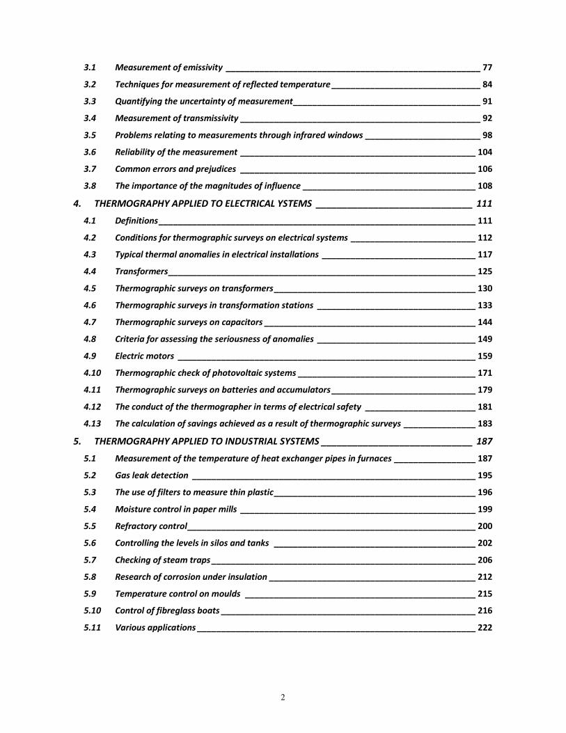
3.1 Measurement of emissivity _____________________________________________________ 77

3.2 Techniques for measurement of reflected temperature _______________________________ 84

3.3 Quantifying the uncertainty of measurement_______________________________________ 91

3.4 Measurement of transmissivity __________________________________________________ 92

3.5 Problems relating to measurements through infrared windows ________________________ 98

3.6 Reliability of the measurement _________________________________________________ 104

3.7 Common errors and prejudices _________________________________________________ 106

3.8 The importance of the magnitudes of influence ____________________________________ 108

4. THERMOGRAPHY APPLIED TO ELECTRICAL YSTEMS ______________________________ 111

4.1 Definitions __________________________________________________________________ 111

4.2 Conditions for thermographic surveys on electrical systems __________________________ 112

4.3 Typical thermal anomalies in electrical installations ________________________________ 117

4.4 Transformers ________________________________________________________________ 125

4.5 Thermographic surveys on transformers __________________________________________ 130

4.6 Thermographic surveys in transformation stations _________________________________ 133

4.7 Thermographic surveys on capacitors ____________________________________________ 144

4.8 Criteria for assessing the seriousness of anomalies _________________________________ 149

4.9 Electric motors ______________________________________________________________ 159

4.10 Thermographic check of photovoltaic systems _____________________________________ 171

4.11 Thermographic surveys on batteries and accumulators ______________________________ 179

4.12 The conduct of the thermographer in terms of electrical safety _______________________ 181

4.13 The calculation of savings achieved as a result of thermographic surveys _______________ 183

5. THERMOGRAPHY APPLIED TO INDUSTRIAL SYSTEMS _____________________________ 187

5.1 Measurement of the temperature of heat exchanger pipes in furnaces _________________ 187

5.2 Gas leak detection ___________________________________________________________ 195

5.3 The use of filters to measure thin plastic __________________________________________ 196

5.4 Moisture control in paper mills _________________________________________________ 199

5.5 Refractory control ____________________________________________________________ 200

5.6 Controlling the levels in silos and tanks __________________________________________ 202

5.7 Checking of steam traps _______________________________________________________ 206

5.8 Research of corrosion under insulation ___________________________________________ 212

5.9 Temperature control on moulds ________________________________________________ 215

5.10 Control of fibreglass boats _____________________________________________________ 216

5.11 Various applications __________________________________________________________ 222

4

1. THE PHYSICAL LAWS OF REFERENCE

1.1 Heat and temperature

Heat is a form of energy that is transferred between two bodies, or between two parts of the same

body, that are found in different thermal conditions.

Heat is therefore energy in transit then: it always flows from the points at higher temperature to

those at a lower temperature, until a thermal equilibrium is reached, that is, until the two bodies

reach the same temperature. Heat is measured in joules (J).

Temperature, however, is an index of molecular agitation.

1.2 Conduction: Fourier's law

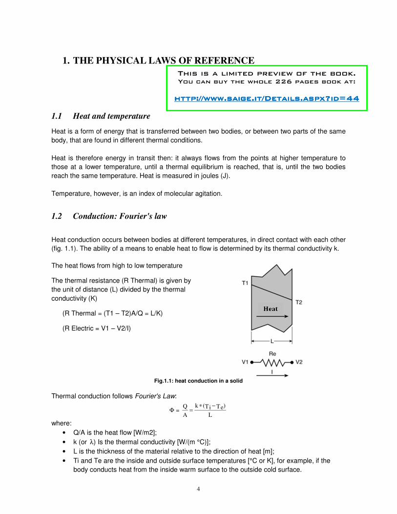
Heat conduction occurs between bodies at different temperatures, in direct contact with each other

(fig. 1.1). The ability of a means to enable heat to flow is determined by its thermal conductivity k.

The heat flows from high to low temperature

The thermal resistance (R Thermal) is given by

the unit of distance (L) divided by the thermal

conductivity (K)

(R Thermal = (T1 – T2)A/Q = L/K)

(R Electric = V1 – V2/I)

Fig.1.1: heat conduction in a solid

Thermal conduction follows Fourier's Law:

Φ = L

)TeTi(k

A

Q −∗=

where:

• Q/A is the heat flow [W/m2];

• k (or λ) Is the thermal conductivity [W/(m °C)];

• L is the thickness of the material relative to the direction of heat [m];

• Ti and Te are the inside and outside surface temperatures [°C or K], for example, if the

body conducts heat from the inside warm surface to the outside cold surface.

This is a limited preview of the book. You can buy the whole 226 pages book at:

http://www.saige.it/Details.aspx?id=44http://www.saige.it/Details.aspx?id=44http://www.saige.it/Details.aspx?id=44http://www.saige.it/Details.aspx?id=44

5

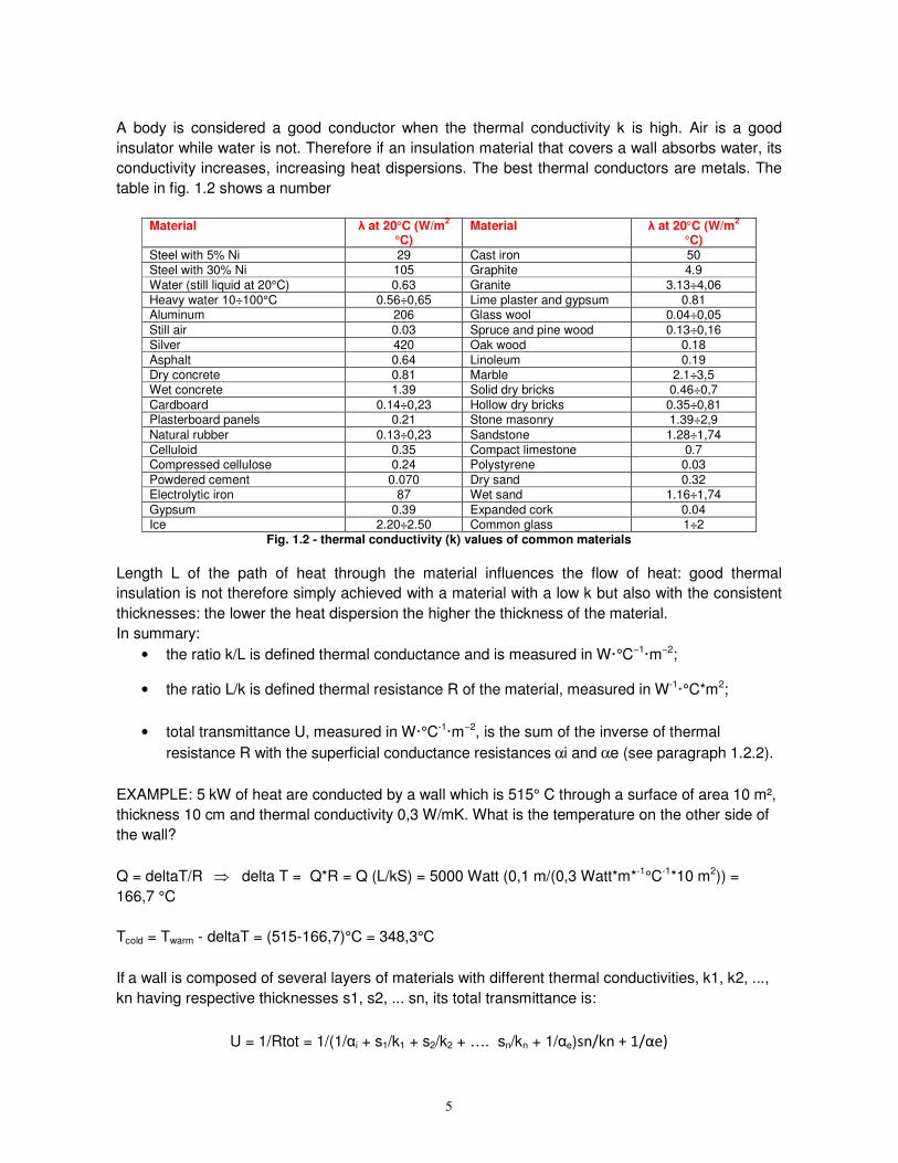
A body is considered a good conductor when the thermal conductivity k is high. Air is a good

insulator while water is not. Therefore if an insulation material that covers a wall absorbs water, its

conductivity increases, increasing heat dispersions. The best thermal conductors are metals. The

table in fig. 1.2 shows a number

Material λ at 20°C (W/m

2

°C) Material λ at 20°C (W/m

2

°C)

Steel with 5% Ni 29 Cast iron 50

Steel with 30% Ni 105 Graphite 4.9

Water (still liquid at 20°C) 0.63 Granite 3.13÷4,06

Heavy water 10÷100°C 0.56÷0,65 Lime plaster and gypsum 0.81 Aluminum 206 Glass wool 0.04÷0,05

Still air 0.03 Spruce and pine wood 0.13÷0,16

Silver 420 Oak wood 0.18

Asphalt 0.64 Linoleum 0.19

Dry concrete 0.81 Marble 2.1÷3,5 Wet concrete 1.39 Solid dry bricks 0.46÷0,7

Cardboard 0.14÷0,23 Hollow dry bricks 0.35÷0,81 Plasterboard panels 0.21 Stone masonry 1.39÷2,9

Natural rubber 0.13÷0,23 Sandstone 1.28÷1,74

Celluloid 0.35 Compact limestone 0.7 Compressed cellulose 0.24 Polystyrene 0.03

Powdered cement 0.070 Dry sand 0.32 Electrolytic iron 87 Wet sand 1.16÷1,74

Gypsum 0.39 Expanded cork 0.04 Ice 2.20÷2.50 Common glass 1÷2

Fig. 1.2 - thermal conductivity (k) values of common materials

Length L of the path of heat through the material influences the flow of heat: good thermal

insulation is not therefore simply achieved with a material with a low k but also with the consistent

thicknesses: the lower the heat dispersion the higher the thickness of the material.

In summary:

• the ratio k/L is defined thermal conductance and is measured in W·°C−1·m−2;

• the ratio L/k is defined thermal resistance R of the material, measured in W-1·°C*m2;

• total transmittance U, measured in W·°C-1·m−2, is the sum of the inverse of thermal

resistance R with the superficial conductance resistances αi and αe (see paragraph 1.2.2).

EXAMPLE: 5 kW of heat are conducted by a wall which is 515° C through a surface of area 10 m²,

thickness 10 cm and thermal conductivity 0,3 W/mK. What is the temperature on the other side of

the wall?

Q = deltaT/R ⇒ delta T = Q*R = Q (L/kS) = 5000 Watt (0,1 m/(0,3 Watt*m*-1°C-1*10 m2)) =

166,7 °C

Tcold = Twarm - deltaT = (515-166,7)°C = 348,3°C

If a wall is composed of several layers of materials with different thermal conductivities, k1, k2, ...,

kn having respective thicknesses s1, s2, ... sn, its total transmittance is:

U = 1/Rtot = 1/(1/αi + s1/k1 + s2/k2 + …. sn/kn + 1/αe)sn/kn + 1/αe)

27

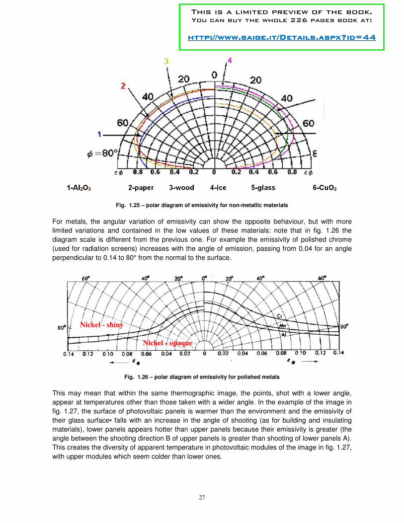
Fig. 1.25 – polar diagram of emissivity for non-metallic materials

For metals, the angular variation of emissivity can show the opposite behaviour, but with more

limited variations and contained in the low values of these materials: note that in fig. 1.26 the

diagram scale is different from the previous one. For example the emissivity of polished chrome

(used for radiation screens) increases with the angle of emission, passing from 0.04 for an angle

perpendicular to 0.14 to 80° from the normal to the surface.

Fig. 1.26 – polar diagram of emissivity for polished metals

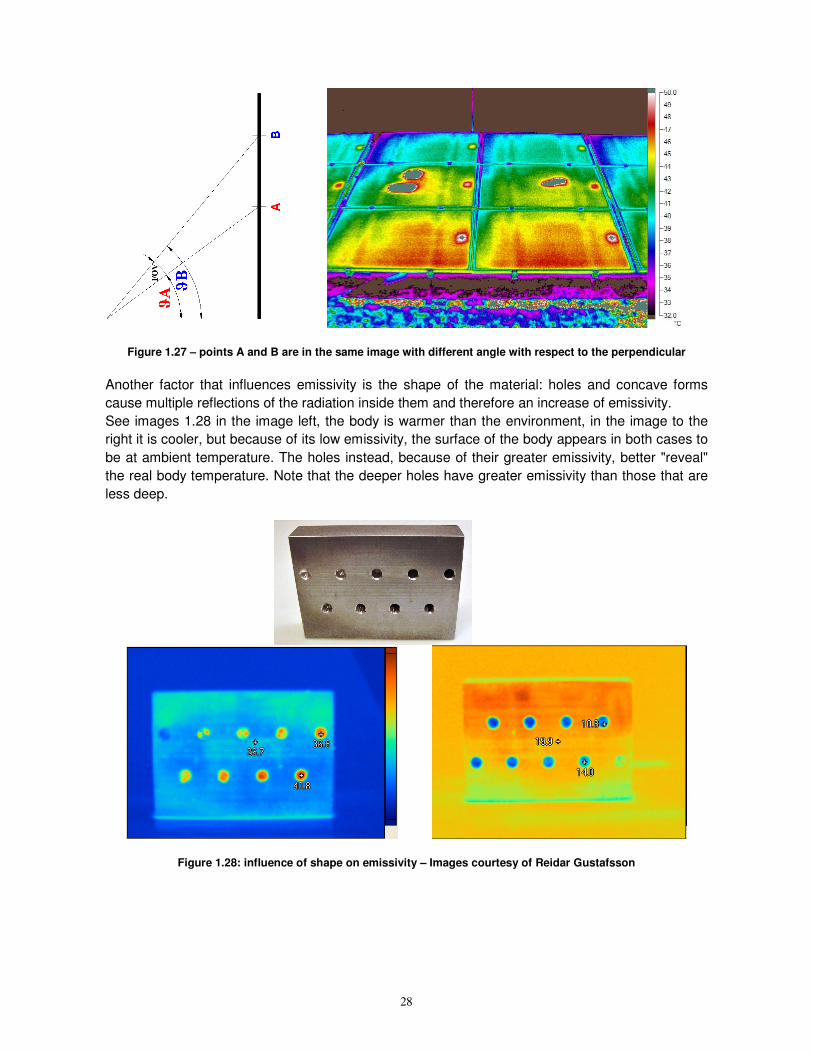
This may mean that within the same thermographic image, the points, shot with a lower angle,

appear at temperatures other than those taken with a wider angle. In the example of the image in

fig. 1.27, the surface of photovoltaic panels is warmer than the environment and the emissivity of

their glass surface• falls with an increase in the angle of shooting (as for building and insulating

materials), lower panels appears hotter than upper panels because their emissivity is greater (the

angle between the shooting direction B of upper panels is greater than shooting of lower panels A).

This creates the diversity of apparent temperature in photovoltaic modules of the image in fig. 1.27,

with upper modules which seem colder than lower ones.

Nickel - shiny

Nickel - opaque



28

Figure 1.27 – points A and B are in the same image with different angle with respect to the perpendicular

Another factor that influences emissivity is the shape of the material: holes and concave forms

cause multiple reflections of the radiation inside them and therefore an increase of emissivity.

See images 1.28 in the image left, the body is warmer than the environment, in the image to the

right it is cooler, but because of its low emissivity, the surface of the body appears in both cases to

be at ambient temperature. The holes instead, because of their greater emissivity, better "reveal"

the real body temperature. Note that the deeper holes have greater emissivity than those that are

less deep.

Figure 1.28: influence of shape on emissivity – Images courtesy of Reidar Gustafsson

77

3. THERMOGRAPHIC MEASUREMENT

As the thermal imaging camera measures a radiance Em which is the sum of the energy emitted

(Ee), reflected (Er ) and eventually transmitted (Et) by the object (if it is not opaque), to determine

the temperature of the object it is necessary (paragraph 2.1.4):

• to subtract from the total energy measured (Em) parts Er and Et to obtain the sole energy

emitted, which is the only one able to provide information on the actual temperature of the

object:

Ee = Em – Er – Et

• to divide the energy emitted for the emissivity ε of the surface of the object in order to

understand which energy a black-body emits (Ecn) that is at the same temperature of the

object (and within the same range of wavelength of the thermal imaging camera, where the

real object is assumed to be grey):

Ecn = Ee / ε

Only once these steps have been addressed is the thermal imaging camera able, by using the

stored calibration curve it contains, to derive the temperature of the object. The calibration curve,

as it is obtained in the laboratory, refers to a black-body, which does not reflect or transmit energy

and has ε = 1: for this reason, it is necessary to determine the energy emitted by a black-body at

the same temperature of the object, eliminating the reflected and transmitted components.

3.1 Measurement of emissivity

There are 5 methods to evaluate emissivity:

1. using standard values (the simplest but least reliable method):

- organic materials have values of between 0.85 and 0.95 approximately

- metals have very variable emissivity: generally low for shiny metals and high for those that

are oxidised and painted

2. using emissivity tables with values reported depending on the wavelength

3. estimating the emissivity from similar objects and searching for a representative sample of

them

4. locally modifying the emissivity of the object with known emissivity finishes (good

procedure), for example, insulating tape, paint or sprays (all methods that bring the

emissivity to approximately ε = 0.96≈0.98)

5. measuring the emissivity using standard procedures (eg. ASTM E-1933).



78

In the following, we will examine the methods for measuring the emissivity of an object. All the

methods require contact with the object and involve modification of the object's temperature to at

least 10°C above ambient temperature to be more reliable (the measurement of a body that is

colder than the environment is most affected by reflected radiation and is therefore more

uncertain).

As the emissivity also depends on the temperature (see section 1.15.3), the methods determine

the emissivity of the object at the temperature at which it is brought for measurement: if in the

situation of actual measurement the object is found to be at a different temperature, its emissivity

may also be different.

In addition, the emissivity found experimentally also depends on the make and model of the

thermal imaging camera used in the test (due to the different wavelength at which several thermal

imaging cameras work even if for example it involves 2 models of thermal imaging cameras

operating in the LW), and also for several measurements made with the same thermal imaging

camera: in fact each measurement consists of 2 measurements (of the reflected temperature and

of the object), each affected by random uncertainties.

In the procedures defined by the ASTM E-1933 American Standard, the material required for the

test is as follows:

1. a controlled environment, with uniform radiant temperature (walls at the same temperature,

for example, air-conditioned room) and without air currents that might produce convective

effects

2. calibrated thermal imaging camera with the possibility of setting emissivity and reflected

temperature

3. a diffuse reflector of infrared radiation (see 3.2.2)

4. a system of heating the object to at least 20°C above ambient temperature

5. a system to bring locally the emissivity of the object to a value that is higher and known, for

the procedure defined in paragraph 3.1.1

6. a calibrated contact thermometer (e.g. thermocouple), for the procedure defined in

paragraph 3.1.2.

In the following paragraphs 3.1.1 and 3.1.2, for performing steps 3, 4 and 5 it is recommended to read paragraph 3.2.2.

3.1.1 Technique using marker of known emissivity

The method of measurement of the emissivity with the marker with known emissivity required by

ASTM E-1933 includes the following steps (fig. 3.1):

1. uniformly heat the object up to a temperature of at least 20°C higher than the ambient

temperature and maintain it at a constant temperature

2. position the thermal imaging camera at the desired distance from the object, focussing on

the area where the emissivity of the object to be measured

3. ensure the diffuse reflector is parallel to the object (see 3.2.2)

4. set the emissivity = 1 in the thermal imaging camera

84

3.2 Techniques for measurement of reflected temperature

The term "reflected temperature" refers to the radiation coming from other solid objects of the

thermal scene that the object to be measured reflects towards the thermal imaging camera.

In this sense the term "temperature" is improper: in fact it is a radiation.

We use the term "reflected temperature" because in its measurement the thermal imaging camera

converts radiation into apparent temperatures. In this sense, the "reflected temperature" is not a

real temperature, but an apparent temperature, measured with the thermal imaging camera setting

a value ε = 1.

In the following, reference will then be made to "apparent reflected apparent temperature" or RAT.

Why is the emissivity set to 1 for measurement of the RAT?

The aim of measuring the RAT is to find the amount of radiation that does not come from the object

but that it reflects towards the thermal imaging camera, in order to be able to exclude it from the

total radiance measured and therefore to be able to determine the actual radiation emitted by the

object and thus, knowing the emissivity, its temperature.

Internally, the thermal imaging camera has a calibration curve that relates the measured irradiation

unit (IU) with the temperature of the black-body used in the laboratory. The calibration curve is then

referred to apparent temperatures (having black-body emissivity equal to 1) and from an object that

does not cause reflections.

In measurements on real objects (outside the laboratory), the radiance coming from the objects

always presents a reflected component, which must be measured and excluded from the

measurement. In measuring the RAT, the real "reflected temperature" is not relevant but an

"apparent reflected temperature" from which, by means of the calibration curve, the reflected

radiation to be subtracted from the total one measured is deduced.

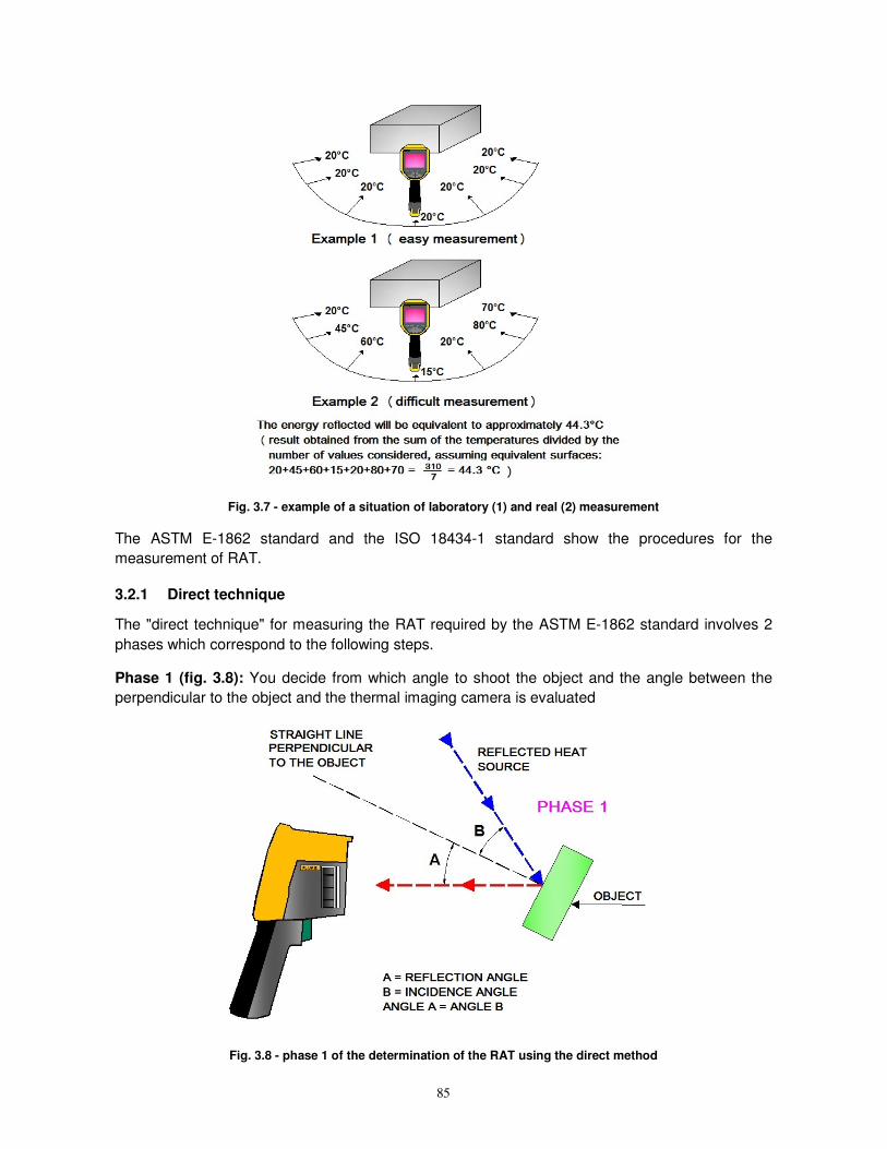
Fig. 3.7 clarifies the difference between the laboratory situation and the real situation: example 1

above shows the desired situation in the laboratory during calibration of the imager, with uniform

radiant temperatures of all the walls. The figure below shows an example of the situation of actual

measurement, which is much more complicated, with bodies at different temperatures that cause

thermal reflections of different entities on the object to be measured.



85

Fig. 3.7 - example of a situation of laboratory (1) and real (2) measurement

The ASTM E-1862 standard and the ISO 18434-1 standard show the procedures for the

measurement of RAT.

3.2.1 Direct technique

The "direct technique" for measuring the RAT required by the ASTM E-1862 standard involves 2

phases which correspond to the following steps.

Phase 1 (fig. 3.8): You decide from which angle to shoot the object and the angle between the

perpendicular to the object and the thermal imaging camera is evaluated

Fig. 3.8 - phase 1 of the determination of the RAT using the direct method

86

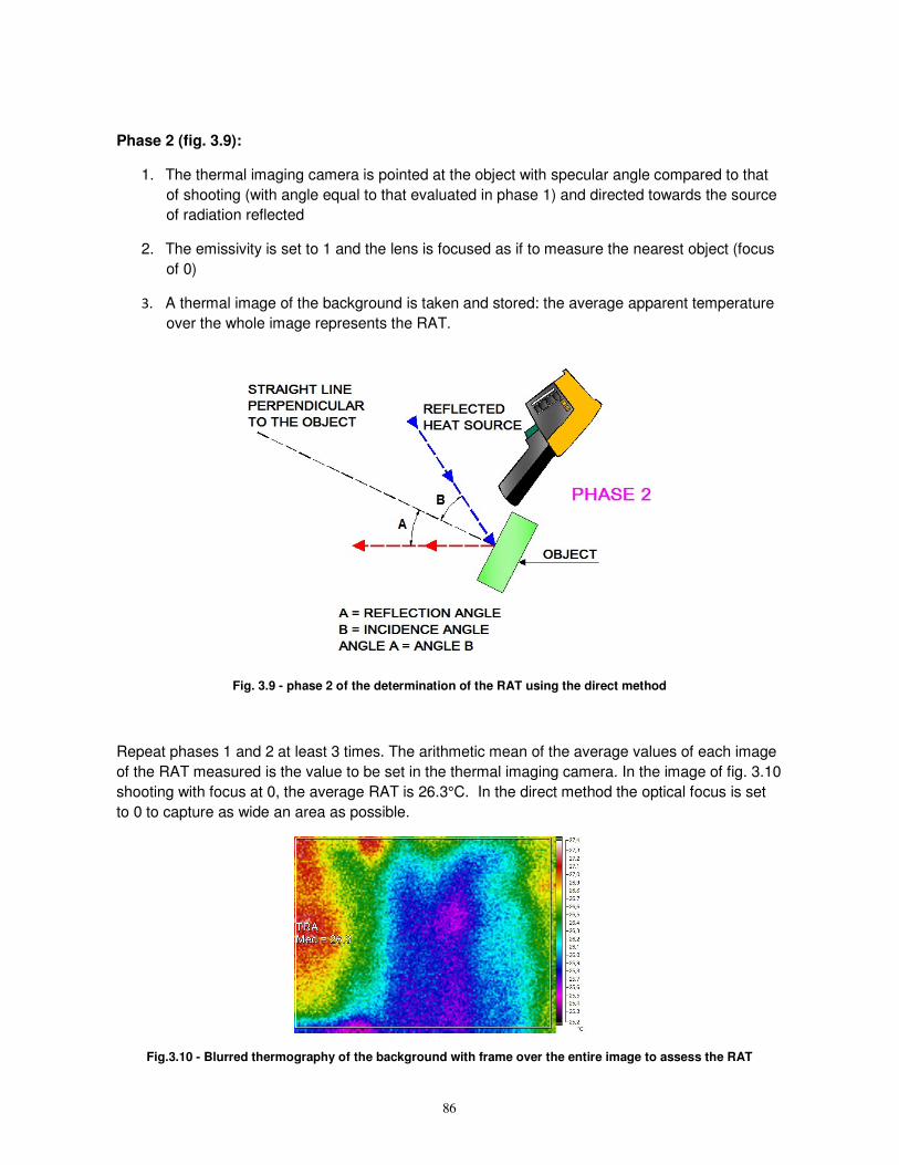
Phase 2 (fig. 3.9):

1. The thermal imaging camera is pointed at the object with specular angle compared to that

of shooting (with angle equal to that evaluated in phase 1) and directed towards the source

of radiation reflected

2. The emissivity is set to 1 and the lens is focused as if to measure the nearest object (focus

of 0)

3. A thermal image of the background is taken and stored: the average apparent temperature

over the whole image represents the RAT.

Fig. 3.9 - phase 2 of the determination of the RAT using the direct method

Repeat phases 1 and 2 at least 3 times. The arithmetic mean of the average values of each image

of the RAT measured is the value to be set in the thermal imaging camera. In the image of fig. 3.10

shooting with focus at 0, the average RAT is 26.3°C. In the direct method the optical focus is set

to 0 to capture as wide an area as possible.

Fig.3.10 - Blurred thermography of the background with frame over the entire image to assess the RAT

116

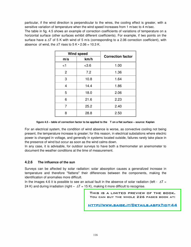
particular, if the wind direction is perpendicular to the wires, the cooling effect is greater, with a

sensitive variation of temperature when the wind speed increases from 1 m/sec to 4 m/sec.

The table in fig. 4.5 shows an example of correction coefficients of variations of temperature on a

horizontal surface (other surfaces exhibit different coefficients). For example, if two points on the

surface have a ∆T of 5 K with wind of 5 m/s (corresponding to a 2.06 correction coefficient), with

absence of wind, the ∆T rises to 5 K • 2.06 = 10.3 K.

Wind speed Correction factor

m/s km/h

<1 <3.6 1.00

2 7.2 1.36

3 10.8 1.64

4 14.4 1.86

5 18.0 2.06

6 21.6 2.23

7 25.2 2.40

8 28.8 2.50

figure 4.5 – table of correction factor to be applied to the T on a flat surface – source: Kaplan

For an electrical system, the condition of wind absence is worse, as convective cooling not being

present, the temperature increase is greater; for this reason, in electrical substations where electric

power is changed in voltage, and generally in systems located outside, failures rarely take place in

the presence of wind but occur as soon as the wind calms down.

In any case, it is advisable, for outdoor surveys to have both a thermometer an anemometer to

document the weather conditions at the time of measurement.

4.2.6 The influence of the sun

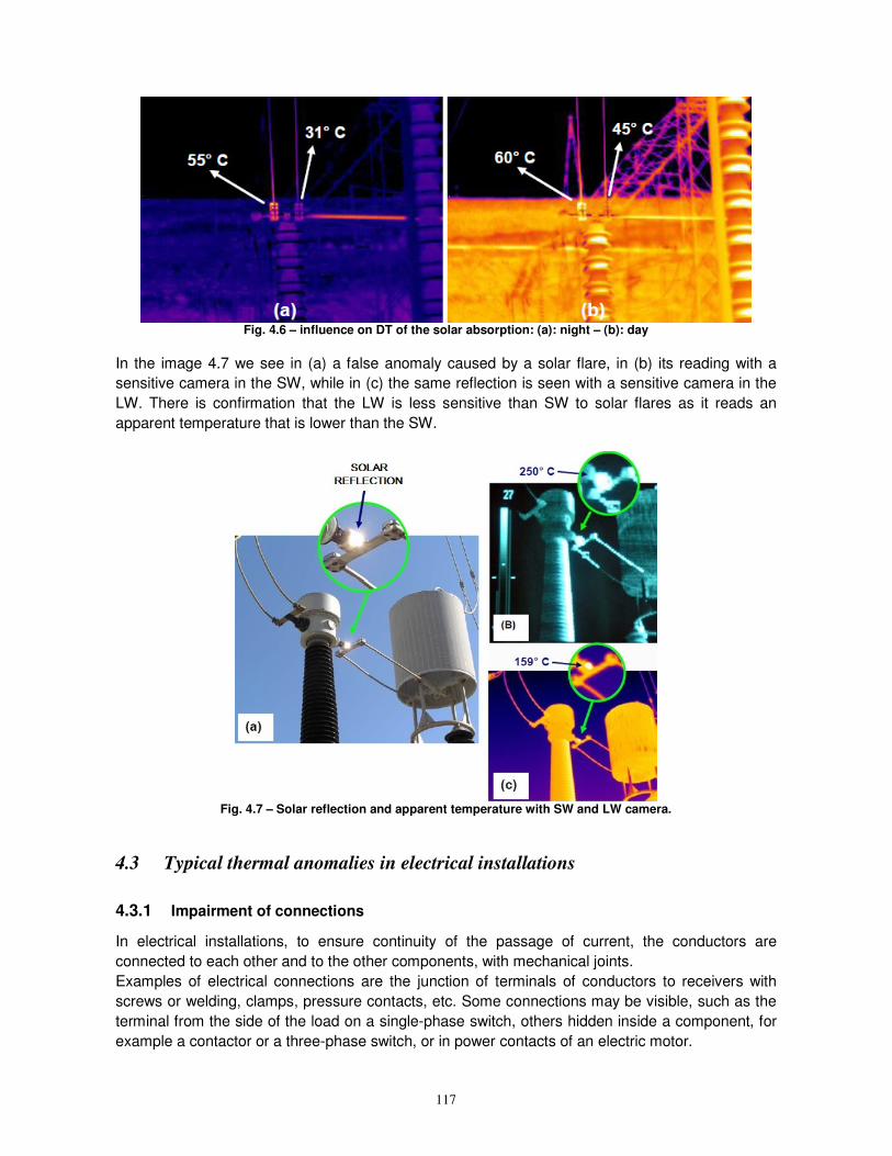
Surveys can be affected by solar radiation: solar absorption causes a generalized increase in

temperature and therefore "flattens" their differences between the components, making the

identification of anomalies more difficult.

In the images 4.6 it is possible to see an actual fault in the absence of solar radiation (left - ∆T =

24 K) and during irradiation (right – ∆T = 15 K), making it more difficult to recognise.



117

Fig. 4.6 – influence on DT of the solar absorption: (a): night – (b): day

In the image 4.7 we see in (a) a false anomaly caused by a solar flare, in (b) its reading with a

sensitive camera in the SW, while in (c) the same reflection is seen with a sensitive camera in the

LW. There is confirmation that the LW is less sensitive than SW to solar flares as it reads an

apparent temperature that is lower than the SW.

Fig. 4.7 – Solar reflection and apparent temperature with SW and LW camera.

4.3 Typical thermal anomalies in electrical installations

4.3.1 Impairment of connections

In electrical installations, to ensure continuity of the passage of current, the conductors are

connected to each other and to the other components, with mechanical joints.

Examples of electrical connections are the junction of terminals of conductors to receivers with

screws or welding, clamps, pressure contacts, etc. Some connections may be visible, such as the

terminal from the side of the load on a single-phase switch, others hidden inside a component, for

example a contactor or a three-phase switch, or in power contacts of an electric motor.

149

power absorbed is all active power. In circuits with utilities that contain coils such as motors,

welding machines, power supply units of fluorescent lamps and transformers, a part of the power

absorbed is committed to excite magnetic circuits and is therefore not used as active power but as

power usually called reactive power.

In industrial facilities, most loads consist of motors and transformers that generate a magnetic field,

which "lower" voltage and current causing the production of reactive energy (expressed in

kVARh). The only "useful" power (able to transform electrical energy in mechanical work) is active

power. Reactive power, can not only be transformed into mechanical work but also causes the

transit into the network of inductive current. This inductive current causes a decrease in the

transport capacity of "useful energy" from the cable as (if we assimilate the cord to a hypothetical

pipe) its presence "steals" space from a certain amount of active energy. Inductive-reactive power

therefore constitutes an additional load for generators, transformers and transmission and

distribution lines, committing the energy supplier to oversize its generators at the expense of

efficiency and also causing a greater drop in line voltage which translates into further active power

losses. To work around this problem, capacitor batteries are inserted in parallel to the motors of

the capacitors (capacitive loads) that counteract the effect of the inductive loads, aiming to bring

into "phase" both voltage and current. For this reason it is called "power factor correction".

For low voltage installations and with committed power greater than 15 kW, Italian regulations set

the following:

• when the average monthly power factor is less than 0.7, the user is obligated to subject the

plant to power factor correction.

• when the average monthly power factor is between 0.7 and 0.9, there is no obligation to

correct the plant but the user pays a penalty for the reactive energy.

• when the average monthly power factor is greater than 1 and less than 0.9, there is no

obligation for power factor correction and no reactive energy fee is payable.

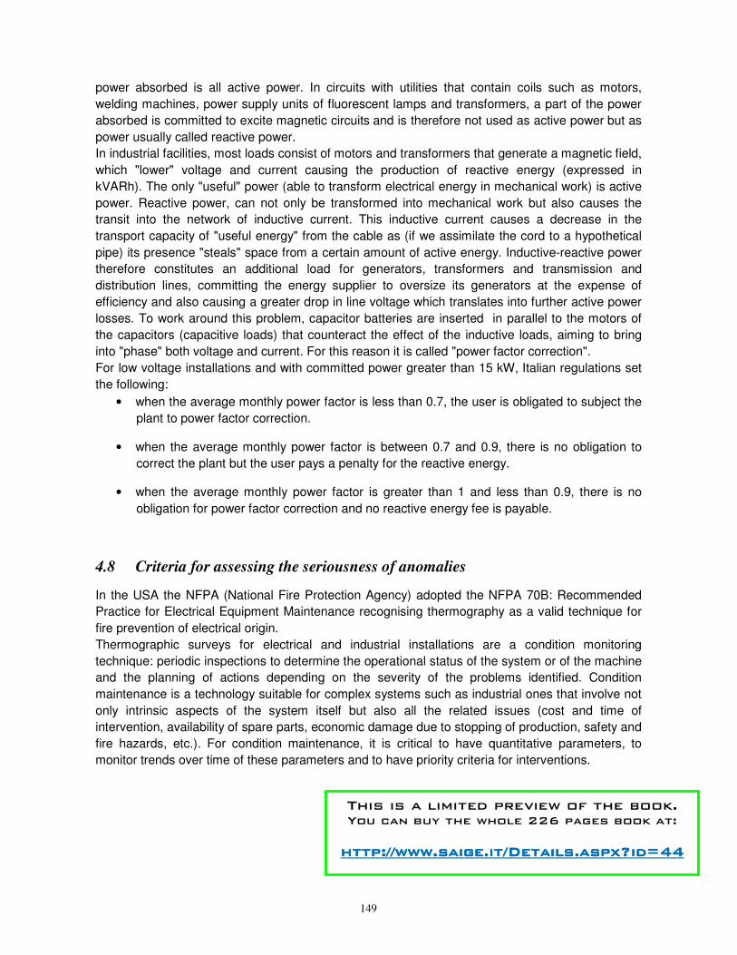
4.8 Criteria for assessing the seriousness of anomalies

In the USA the NFPA (National Fire Protection Agency) adopted the NFPA 70B: Recommended

Practice for Electrical Equipment Maintenance recognising thermography as a valid technique for

fire prevention of electrical origin.

Thermographic surveys for electrical and industrial installations are a condition monitoring

technique: periodic inspections to determine the operational status of the system or of the machine

and the planning of actions depending on the severity of the problems identified. Condition

maintenance is a technology suitable for complex systems such as industrial ones that involve not

only intrinsic aspects of the system itself but also all the related issues (cost and time of

intervention, availability of spare parts, economic damage due to stopping of production, safety and

fire hazards, etc.). For condition maintenance, it is critical to have quantitative parameters, to

monitor trends over time of these parameters and to have priority criteria for interventions.



150

Thermography is used not only to prevent catastrophic events but is especially useful as predictive

maintenance to avoid plant stoppages that would cause interruptions of production with much more

expensive consequences than simple repair of the fault.

In Italy, ENEL has for many years recognised the effectiveness of thermography and has an

operating procedure for thermographic surveys of transformation cabins and substations to prevent

blackouts.

It is essential to carry out the survey in the presence of adequate current load (the foreign technical

standards, that are not unique, refer to 30%, 40% or 50% of the nominal load) to be sure that the

thermal anomalies occur with temperature changes that are easily detectable and uniquely

interpretable.

The foreign technical standards have different criteria for assessing the gravity of an electrical

anomaly: these are always related to its temperature. This can be "equivalent temperature" or the

temperature difference between the component and the temperature of the air, or between the

temperature difference between the component and a similar component that is in the same

operating conditions.

4.8.1 Anomaly indices based on the correct temperature of the component

This criterion is based on the component temperature at full load at a fixed ambient temperature.

To determine if the temperature of the component, thermographically detected, is less than that

tolerable, two methods are used.

To apply this, you need to know:

• the thermal conductivity: if the fault is very high, it may dissipate heat efficiently by

conduction towards other components. For this reason, certain standards allow in this case

application of the lowest values of 2 to the exponent of which the current value is elevated

in the formula of the Joule effect (section 4.2.1); in the absence of information, with the aim

of operating safely, thermal conductivity is not considered and 2 is always applied as

exponent

• the temperature at the maximum full load that can be tolerated by the component in

question, and the relevant reference temperature to which it refers.

• the maximum load

• the load at the time of the inspection (e.g. measuring it by means of an amperometric

clamp)

• the ambient temperature at the time of the inspection (for method 2)

• the reference ambient temperature (for method 2).

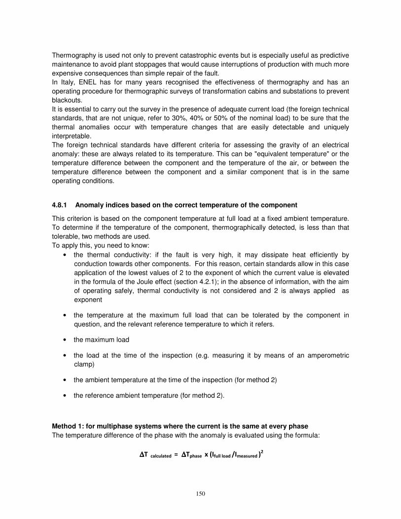
Method 1: for multiphase systems where the current is the same at every phase

The temperature difference of the phase with the anomaly is evaluated using the formula:

∆ ∆ ∆ ∆T calculated = ∆ ∆ ∆ ∆Tphase x (Ifull load /Imeasured )2

151

Application example: during a thermographic survey on 3 electric cables with load of 30 A, a

temperature is recorded with the thermal imaging camera that is 3°C higher than the others on the

contract of one of these. The full load current is 100 A. A full load ∆Tcalculated is:

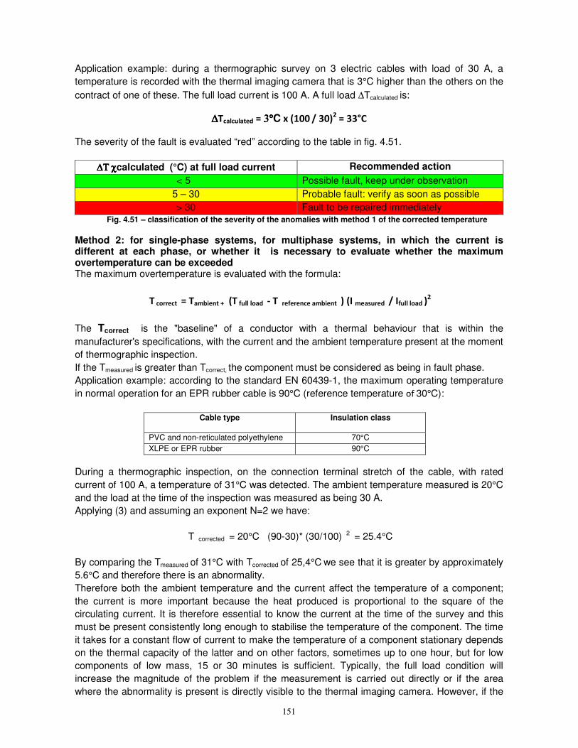
∆∆∆∆Tcalculated = 3°3°3°3°C x (100 / 30)2 = 33°C

The severity of the fault is evaluated “red” according to the table in fig. 4.51.

∆Τ χ∆Τ χ∆Τ χ∆Τ χcalculated (°C) at full load current Recommended action

< 5 Possible fault, keep under observation

5 – 30 Probable fault: verify as soon as possible

> 30 Fault to be repaired immediately Fig. 4.51 – classification of the severity of the anomalies with method 1 of the corrected temperature

Method 2: for single-phase systems, for multiphase systems, in which the current is different at each phase, or whether it is necessary to evaluate whether the maximum overtemperature can be exceeded The maximum overtemperature is evaluated with the formula:

T correct = Tambient + (T full load - T reference ambient ) (I measured / Ifull load )2

The Tcorrect is the "baseline" of a conductor with a thermal behaviour that is within the

manufacturer's specifications, with the current and the ambient temperature present at the moment

of thermographic inspection.

If the Tmeasured is greater than Tcorrect, the component must be considered as being in fault phase.

Application example: according to the standard EN 60439-1, the maximum operating temperature

in normal operation for an EPR rubber cable is 90°C (reference temperature of 30°C):

Cable type Insulation class

PVC and non-reticulated polyethylene 70°C

XLPE or EPR rubber 90°C

During a thermographic inspection, on the connection terminal stretch of the cable, with rated

current of 100 A, a temperature of 31°C was detected. The ambient temperature measured is 20°C

and the load at the time of the inspection was measured as being 30 A.

Applying (3) and assuming an exponent N=2 we have:

T corrected = 20°C (90-30)* (30/100) 2 = 25.4°C

By comparing the Tmeasured of 31°C with Tcorrected of 25,4°C we see that it is greater by approximately

5.6°C and therefore there is an abnormality.

Therefore both the ambient temperature and the current affect the temperature of a component;

the current is more important because the heat produced is proportional to the square of the

circulating current. It is therefore essential to know the current at the time of the survey and this

must be present consistently long enough to stabilise the temperature of the component. The time

it takes for a constant flow of current to make the temperature of a component stationary depends

on the thermal capacity of the latter and on other factors, sometimes up to one hour, but for low

components of low mass, 15 or 30 minutes is sufficient. Typically, the full load condition will

increase the magnitude of the problem if the measurement is carried out directly or if the area

where the abnormality is present is directly visible to the thermal imaging camera. However, if the

187

5. THERMOGRAPHY APPLIED TO INDUSTRIAL SYSTEMS

5.1 Measurement of the temperature of heat exchanger pipes in furnaces

Measurement of the temperature of heat exchangers in furnaces is one of the most difficult

thermographic applications because:

• the temperature of the pipes, while very high, is lower than the internal temperature of the

walls of the furnace (which is the reflected temperature during measurement of tubes):

essentially you are then trying to measure a cold object in a hot environment

• there is the problem of radiation absorption due to the presence of combustion gases inside

furnace, which preferably requires a MW camera with 3.9 micron filter

• there is uncertainty regarding the emissivity value of the pipes.

However, it involves a valid application, also from a qualitative perspective (i.e. without a correct

temperature measurement), due to the economic importance of these systems and the

consequences for safety in the event of faults with them.

The thermographic images provide information on areas of overheating, on the thermal imbalances

and on the areas of formation of deposit deposits inside (called coke) and outside (called scale) of

the pipe surfaces.

Corrective actions taken as a result of the thermographic survey aim to achieve heating of the

product that is as regular as possible. The thermographic method of inspecting refinery furnace

pipes therefore allows correction of the effects of non-uniform flow and thus the opportunity to act

in the presence of combustion problems by correctly adjusting the fuel ratios and optimizing the

thermal load of the furnace (increasing or decreasing the heating).

Most surveys on furnaces are conducted when the entire internal area of the furnace present

neutral or negative pressure difference conditions relative to the outside such that the external air

is sucked back inside and especially resulting in a situation where the products of combustion

cannot be expelled outwards towards the thermographer, who "peeks" inside through a spy hole.

Stringent safety procedures and preliminary meetings are necessary to ensure that the internal

pressure of the furnace is never positive during the thermographic survey.

Certain thermal imaging cameras that can be used in high temperature applications such as

surveys in furnaces are equipped with a lens temperature measurement function that warns the

operator when the lens is at the maximum temperature that it is able to withstand: Germanium

lenses can become almost opaque at high temperatures.

5.1.1 Introduction

Petrochemical furnaces are heat exchangers where the energy developed by the combustion of

gas or oil is transferred to the circulating fluid in the internal pipes. The fluid has a known inlet

temperature and its outgoing temperature must be such as to meet the demands of the industrial

process downstream of the furnace. Energy losses, compared to the total heat developed by

combustion, mainly occur in exhaust gases and through the walls of the furnace.



188

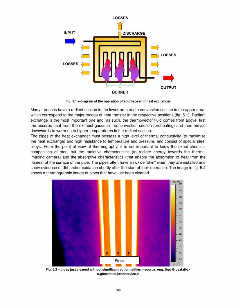
Fig. 5.1 – diagram of the operation of a furnace with heat exchanger

Many furnaces have a radiant section in the lower area and a convection section in the upper area,

which correspond to the major modes of heat transfer in the respective positions (fig. 5.1). Radiant

exchange is the most important one and, as such, the thermovector fluid comes from above, first

the absorbs heat from the exhaust gases in the convection section (preheating) and then moves

downwards to warm up to higher temperatures in the radiant section.

The pipes of the heat exchanger must possess a high level of thermal conductivity (to maximise

the heat exchange) and high resistance to temperature and pressure, and consist of special steel

alloys. From the point of view of thermography, it is not important to know the exact chemical

composition of steel but the radiative characteristics (to radiate energy towards the thermal

imaging camera) and the absorptive characteristics (that enable the absorption of heat from the

flames) of the surface of the pipe. The pipes often have an oxide "skin" when they are installed and

show evidence of dirt and/or oxidation shortly after the start of their operation. The image in fig. 5.2

shows a thermographic image of pipes that have just been cleaned.

Fig. 5.2 – pipes just cleaned without significant abnormalities – source: eng. Ugo Giosafatto -

[email protected]

Pipes

200

Fig. 5.15 - paper reel wet section due to a water leak in the process – source: www.fluke.it

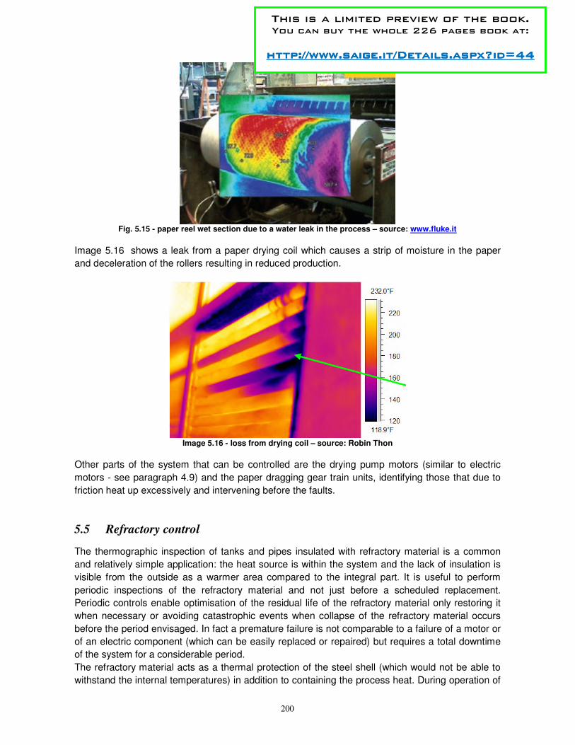
Image 5.16 shows a leak from a paper drying coil which causes a strip of moisture in the paper

and deceleration of the rollers resulting in reduced production.

Image 5.16 - loss from drying coil – source: Robin Thon

Other parts of the system that can be controlled are the drying pump motors (similar to electric

motors - see paragraph 4.9) and the paper dragging gear train units, identifying those that due to

friction heat up excessively and intervening before the faults.

5.5 Refractory control

The thermographic inspection of tanks and pipes insulated with refractory material is a common

and relatively simple application: the heat source is within the system and the lack of insulation is

visible from the outside as a warmer area compared to the integral part. It is useful to perform

periodic inspections of the refractory material and not just before a scheduled replacement.

Periodic controls enable optimisation of the residual life of the refractory material only restoring it

when necessary or avoiding catastrophic events when collapse of the refractory material occurs

before the period envisaged. In fact a premature failure is not comparable to a failure of a motor or

of an electric component (which can be easily replaced or repaired) but requires a total downtime

of the system for a considerable period.

The refractory material acts as a thermal protection of the steel shell (which would not be able to

withstand the internal temperatures) in addition to containing the process heat. During operation of



201

the system, it is subjected to high thermal stress which also involves cycles of expansion and

contraction, as well as internal pressures.

If the receptacle or conduit is under pressure, the temperature resistance of the metal suffers and

falls considerably.

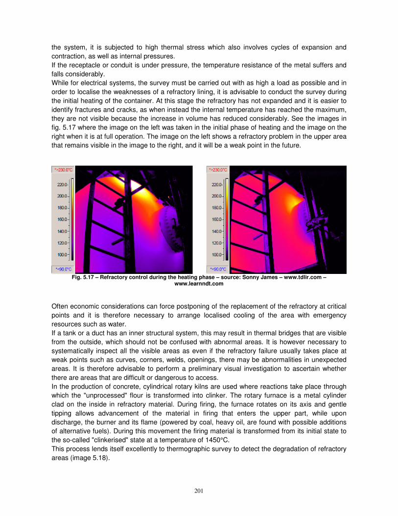
While for electrical systems, the survey must be carried out with as high a load as possible and in

order to localise the weaknesses of a refractory lining, it is advisable to conduct the survey during

the initial heating of the container. At this stage the refractory has not expanded and it is easier to

identify fractures and cracks, as when instead the internal temperature has reached the maximum,

they are not visible because the increase in volume has reduced considerably. See the images in

fig. 5.17 where the image on the left was taken in the initial phase of heating and the image on the

right when it is at full operation. The image on the left shows a refractory problem in the upper area

that remains visible in the image to the right, and it will be a weak point in the future.

Fig. 5.17 – Refractory control during the heating phase – source: Sonny James – www.tdlir.com –

www.learnndt.com

Often economic considerations can force postponing of the replacement of the refractory at critical

points and it is therefore necessary to arrange localised cooling of the area with emergency

resources such as water.

If a tank or a duct has an inner structural system, this may result in thermal bridges that are visible

from the outside, which should not be confused with abnormal areas. It is however necessary to

systematically inspect all the visible areas as even if the refractory failure usually takes place at

weak points such as curves, corners, welds, openings, there may be abnormalities in unexpected

areas. It is therefore advisable to perform a preliminary visual investigation to ascertain whether

there are areas that are difficult or dangerous to access.

In the production of concrete, cylindrical rotary kilns are used where reactions take place through

which the "unprocessed" flour is transformed into clinker. The rotary furnace is a metal cylinder

clad on the inside in refractory material. During firing, the furnace rotates on its axis and gentle

tipping allows advancement of the material in firing that enters the upper part, while upon

discharge, the burner and its flame (powered by coal, heavy oil, are found with possible additions

of alternative fuels). During this movement the firing material is transformed from its initial state to

the so-called "clinkerised" state at a temperature of 1450°C.

This process lends itself excellently to thermographic survey to detect the degradation of refractory

areas (image 5.18).

216

Fig. 5.35 – installation of the thermal imaging camera on a tripod in front of the mould to be monitored – source:

www.saige.it

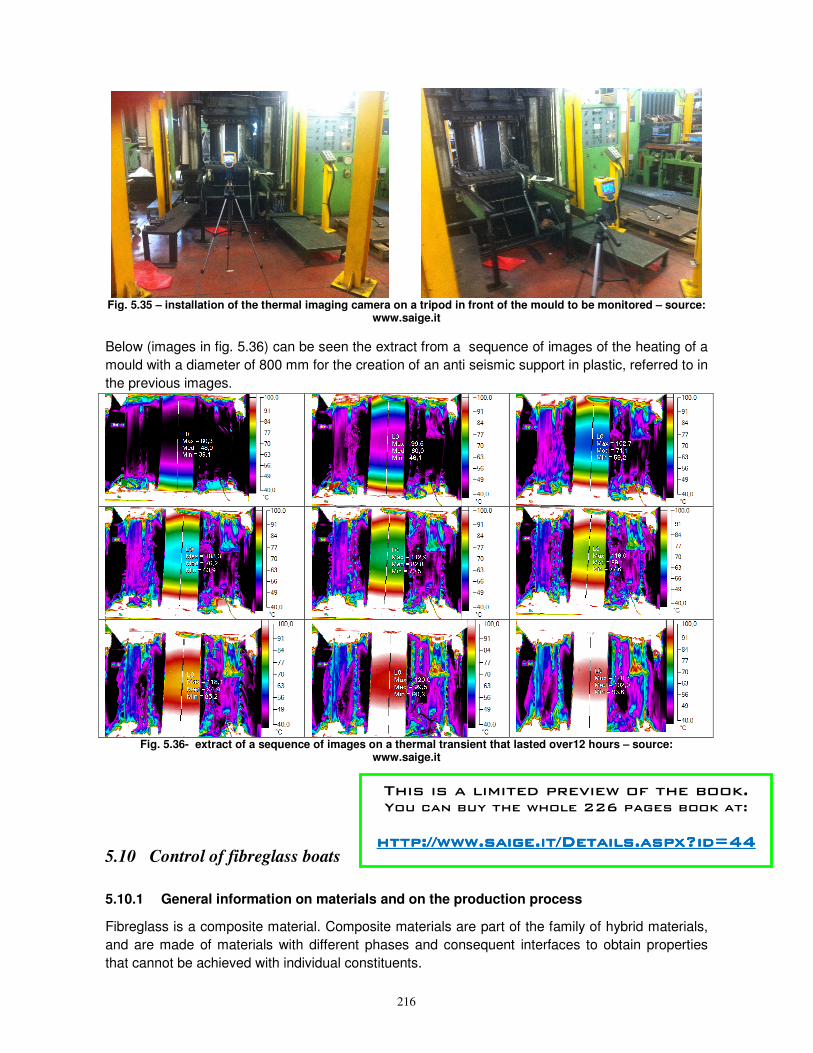
Below (images in fig. 5.36) can be seen the extract from a sequence of images of the heating of a

mould with a diameter of 800 mm for the creation of an anti seismic support in plastic, referred to in

the previous images.

Fig. 5.36- extract of a sequence of images on a thermal transient that lasted over12 hours – source: www.saige.it

5.10 Control of fibreglass boats

5.10.1 General information on materials and on the production process

Fibreglass is a composite material. Composite materials are part of the family of hybrid materials,

and are made of materials with different phases and consequent interfaces to obtain properties

that cannot be achieved with individual constituents.



217

Fibreglass is made from glass fibre strands applied in crossed layers that are distributed by

infusing them with constituted resin usually from a solution of polyester in a monomer (styrene).

The monomer in the presence of a catalyst and an accelerant, forms with the polyester chain a

three-dimensional lattice (polymerisation) with passage of the resin from the liquid state to the solid

state.

To improve the quality of the interface between the glass fibres and the resin, it is necessary to

improve the chemical compatibility between the 2 materials, thus the fibres may be treated with

coatings (called finishes).

Another secondary material used in the production process of fibreglass hulls is "gelcoat ", a

varnish composed of organic macromolecules (polyester or pigmented epoxy resins) that are

spread for staining and protection of the mould.

The realisation of a fibre-glass hull involves the following steps:

• the creation of a precise and solid wooden model

• treatment of the model with "gelcoat", sanding and polishing, following treatment with wax release agents to promote the detachment and the subsequent moulding which will be performed over this.

• the spreading of a further layer of gelcoat for moulds, drying, and start of the deposition of the cross-sheeting of glass fibre in increasing weight with their impregnation with resin and the use of rollers to ensure their perfect grip and to remove air bubbles

• insertion into the mould, with mesh network design, of structural stiffening elements in expanded polyurethane or wood, and metal plates for the fixing of the support frame

• removal of the mould from the wooden model and its finish with gelcoat of the thickness from 0.5 to 0.8 mm: a thickness that is too low would not complete polymerisation of the resin and would not guarantee adequate coverage of the surface; high and poorly distributed thickness could encourage the formation of cracks or deformations due to differing polymerisation times

• start of the production process of the actual artefact from the treated surface of the mould: the glass fibre MAT must be adhered to the resin surface to remove the air bubbles trapped in the resin, which would then promote the emergence of pockets by osmosis (blistering)

• internal strengthening of the artefact with reinforcement elements in foam or wood and the insertion of structural bulkheads (marine plywood panels inserted in a perpendicular form to the major axis of the hull)

• removal of the product from the mould and its completion with the cover and superstructure.

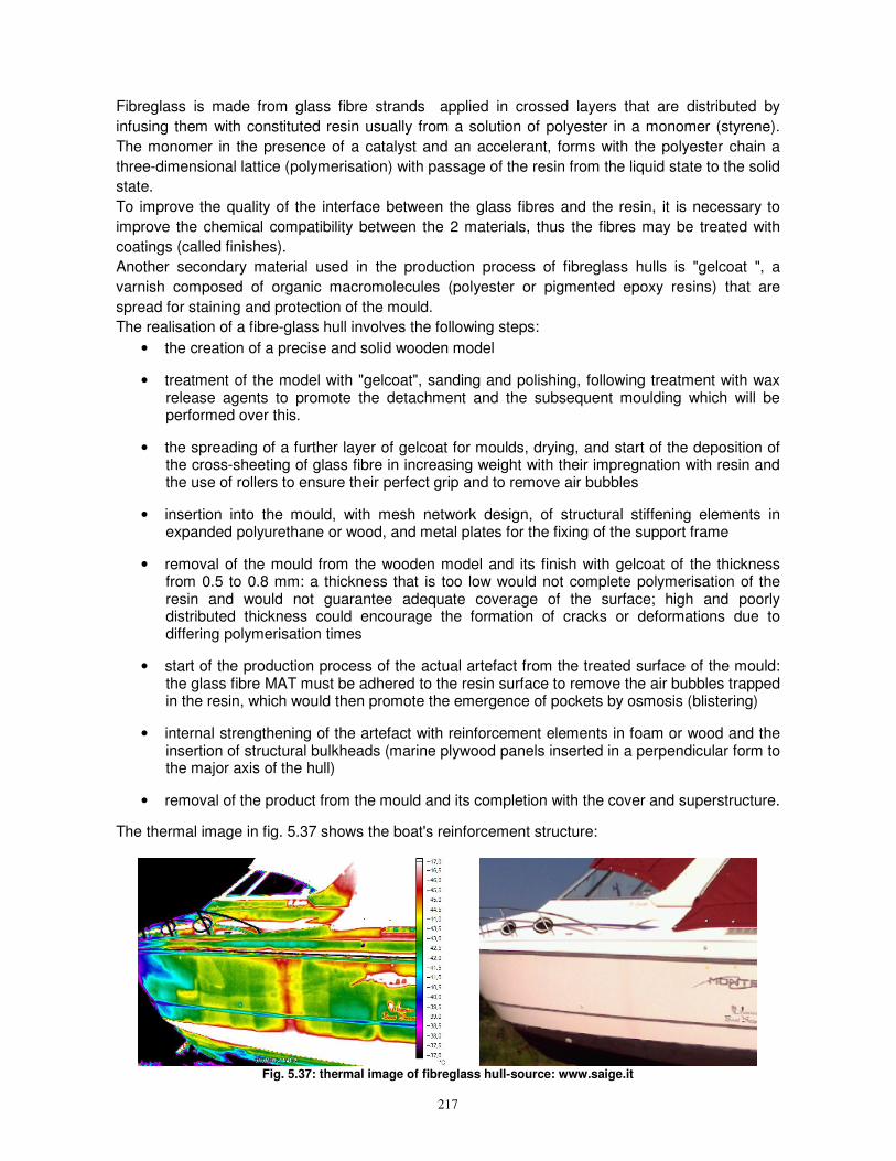
The thermal image in fig. 5.37 shows the boat's reinforcement structure:

Fig. 5.37: thermal image of fibreglass hull-source: www.saige.it

Documents

Infrared thermography 230 pages ebook – electrical and industrial applications