INFRARED SPECTROSCOPY ON MINERALS AND ROCKSCHRIS HECKER (ITC)JULY 2013

INTRO: CHRIS HECKER

CV B.Sc. Earth Sciences (1996) M.Sc. Earth Sciences (1999) University of Basel, Switzerland PhD Thermal RS (2012) ITC

Lecturer Geologic RemoteSensing (70%)

Researcher Geologic RemoteSensing (30%)

Areas of interest: Geologic RS Thermal RS Imaging Spectrometry

Email: c.a.hecker@utwente.nl

INTRO UT-ITC (IN A NUTSHELL)

Mission:development and transfer of knowledge in geo-information science and earth observation

Academic level:PhD/MSc/Master/Postgraduate Diploma

Target group:young and mid-career professionals, and scientists from developing and emerging countries, increasingly professionalsfrom industrialised countries

Frameworkinternational development cooperation

OUTLINE OF LECTURE

SWIR vs TIR Emissivity spectra of Minerals and Rocks Ground-based setups Laboratory Field Mapping methods Case study: TIR+PLSR

THERMAL INFRAREDONE OF THE TOOLS IN THE MODERN EARTH SCIENTIST’S TOOLBOX

K Th U

Radiated energy

The bonds in a molecule or crystal lattice are like springs with attached weights: the whole system can vibrate

Different types of vibration possible Each have different Energy levels Combination of absorption features

can be diagnostic Examples: Al-OH, 2.20 µm Mg-OH, 2.3 µm Ca-CO3, 2.32-2.35 µm Si-O, ~ 9-10 µm

FUNDAMENTAL VIBRATIONAL FREQUENCIES

Stretching

AsymetricStretching

Bending

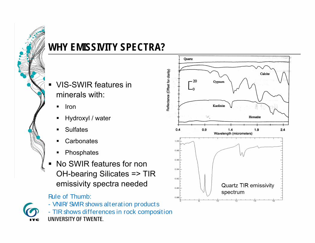
VIS-SWIR features in minerals with: Iron

Hydroxyl / water

Sulfates

Carbonates

Phosphates

No SWIR features for non OH-bearing Silicates => TIR emissivity spectra needed

WHY EMISSIVITY SPECTRA?

Rule of Thumb:- VNIR/SWIR shows alteration products- TIR shows differences in rock composition

OUTLINE OF LECTURE

SWIR vs TIR Emissivity spectra of Minerals and Rocks Ground-based setups Laboratory Field Mapping methods Case study: TIR+PLSR

Reststrahlen feature Strong reflection peak / emission minimum due to fast change

in refractive index and center of strong absorption band. Causes emissivity low Shape is diagnostic for silicates and other minerals

Christiansen frequency Wavelengths where refractive index is close to unity => little

scattering If not in absorption band, causes high transmission and low

reflectance Visible as emissivity maxima in spectra

TYPICAL MINERAL SPECTRA

Mineral (transmission) spectra showing: Christiansen features (up

arrows) Reststrahlen features

(down arrows) Positions shift to longer

wavelengths with decreasing Si-O4tetrahedra polymerization.

TYPICAL MINERAL SPECTRA (CONT’D)

Source: Elachi and van Zyl (2006)

TYPICAL ROCK SPECTRA

Rock spectra usually more complex than mineral spectra

Rock spectra combine features of their main mineralogy

Acidic rocks show reststrahlenband at lower wavelength than basic rocks

Change in emissivity minimum can be used for mapping igneous rocks of variable SiO2 content

• Source: Sabins (1997)

TYPICAL ROCK SPECTRA (CONT’D)

Multi-band thermal systems can help distinguish different rock types and compositions

Vertical lines and numbers indicate 6 bands of the Thermal Infrared Multispectral Scanner (TIMS)

• Source: Drury (2001)

TYPICAL ROCK SPECTRA (CONT’D)

What can we do with it in rock / soil mapping?

Christiansen frequency Exact position not diagnostic in mixtures

Generally high emissivity around 7.5 μm (and 12 μm) useful in TεS.

Reststrahlen feature General position / shape can give hint in multispectral mapping (e.g.,

silica%).

“Deciphering” of reststrahlen feature used for quantitative analysis in spectroscopy (e.g., PLSR or unmix)

Reststrahlen feature of rocks are great for practicing field spectroscopy (before attempting e.g., plants)

TYPICAL ROCK SPECTRA (CONT’D)

Spectral contrast of rocks much higher than in soils or vegetation Example of DHR spectra from ASTER speclib

Source: Hecker et al (2013) Thermal Infrared Spectroscopy in the Laboratory and Field in Support of Land Surface Remote Sensing, in “Thermal Infrared Remote Sensing”, Springer.

OUTLINE OF LECTURE

SWIR vs TIR Emissivity spectra of Minerals and Rocks Ground-based setups Laboratory Field Mapping methods Case study: TIR+PLSR

THE SPEC LAB FAMILY PORTRAIT

LABORATORY FTIR BRUKER & DRIFT

TYPICAL LAB SPECTROMETER WITH DIFFUSE REFLECTANCE (DRIFT) SETUP

Source +InterferometeDetector

Sample

Bruker FTIR spectrometer DRIFT accessory forsmall samples

LABORATORY – SAMPLE CONSIDERATIONS

-Designed for small powder samples-Sampling spot and space too small for most geologic samples

LABORATORY – GEOMETRY CONSIDERATIONS

Sample size Comparison to Rtra

Transmission Bi-dir refl Dir-hem refl Emission

Quantitative comparison with RS data: DHR or Emission only

Emission: careful temperature control of sample needed

Source: Hecker et al (2010); van Ruitenbeek (2007)

LABORATORY – GEOMETRY CONSIDERATIONS (CONT’D)

Same Albite sample

Measured with DRIFT, DHR, transmission.

Qualitatively similar

Quantitatively different(wavelength shifts, relative feature depths … etc.)

Source: Hecker et al (2010)

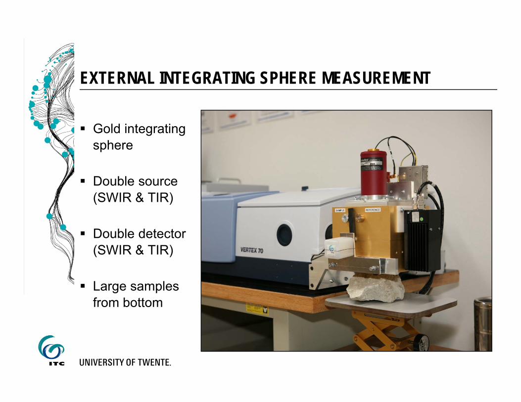
Gold integrating sphere

Double source (SWIR & TIR)

Double detector (SWIR & TIR)

Large samples from bottom

EXTERNAL INTEGRATING SPHERE MEASUREMENT

EXTERNAL INTEGRATING SPHERE MEASUREMENT (CONT’D)

Directional – hemispherical reflectance measurements

Source: Hecker et al (2011)

EXTERNAL INTEGRATING SPHERE MEASUREMENT (CONT’D)

Similar setups at JPL (top left), Geologic Survey Japan (top right)and USGS Reston (bottom center). Photo credit GSJ: R. Hewson

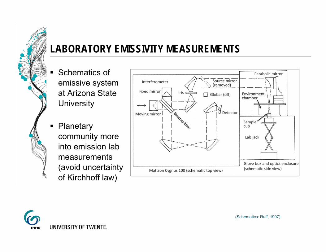
LABORATORY EMISSIVITY MEASUREMENTS

Schematics of emissive system at Arizona State University

Planetary community more into emission lab measurements (avoid uncertainty of Kirchhoff law)

(Schematics: Ruff, 1997)

PITTSBURGH EMISSIVE LAB SPECTROMETER

Prof. Mike Ramsey (formerly ASU)

Emission system based on ASU but further developed

Low temp (80C) and high furnace for high temp (up to 1200C)

Measurement of emissivity changes when rocks melt

FurnaceSample lift

80C Samplehousing

Entry portFTIR

OUTLINE OF LECTURE

SWIR vs TIR Emissivity spectra of Minerals and Rocks Ground-based setups Laboratory Field Mapping methods Case study: TIR+PLSR

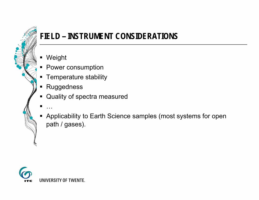
FIELD – INSTRUMENT CONSIDERATIONS

Weight Power consumption Temperature stability Ruggedness Quality of spectra measured … Applicability to Earth Science samples (most systems for open

path / gases).

FIELD – STARTING POINT 1 - µ-FTIR

Pro: Quite light (ca. 7 kg) Low power consumption Designed with ES in mind

(down-looking) Ready-to-go system

Con: Resolution limited Speed of measurement suite Portability OK but not ideal Not rugged Not certified for Europe

Photo source: Richard Bedell, Auex.com

FIELD – STARTING POINT 2 – EMISSION FTIR

Pro: High resolution Good quality of spectra

(high throughput) Rugged

Con: High power consumption Weight! Made for open path

emission measurements. Need specific foreoptics

Photo source: C. Oppenheimer

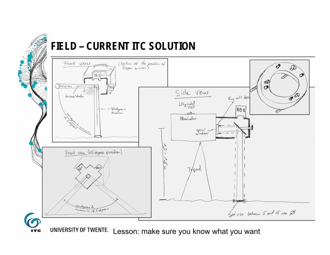
FIELD – CURRENT ITC SOLUTION

Lesson: make sure you know what you want

FIELD – CURRENT ITC SOLUTION (CONT’D)

WITH CUSTOMIZED FOREOPTICS

MIDAC Illuminator M4401

Non-hygroscopic ZnSe optics

Heavy duty, sealed cast aluminium housing (ca 15kg)

lN2 cooled

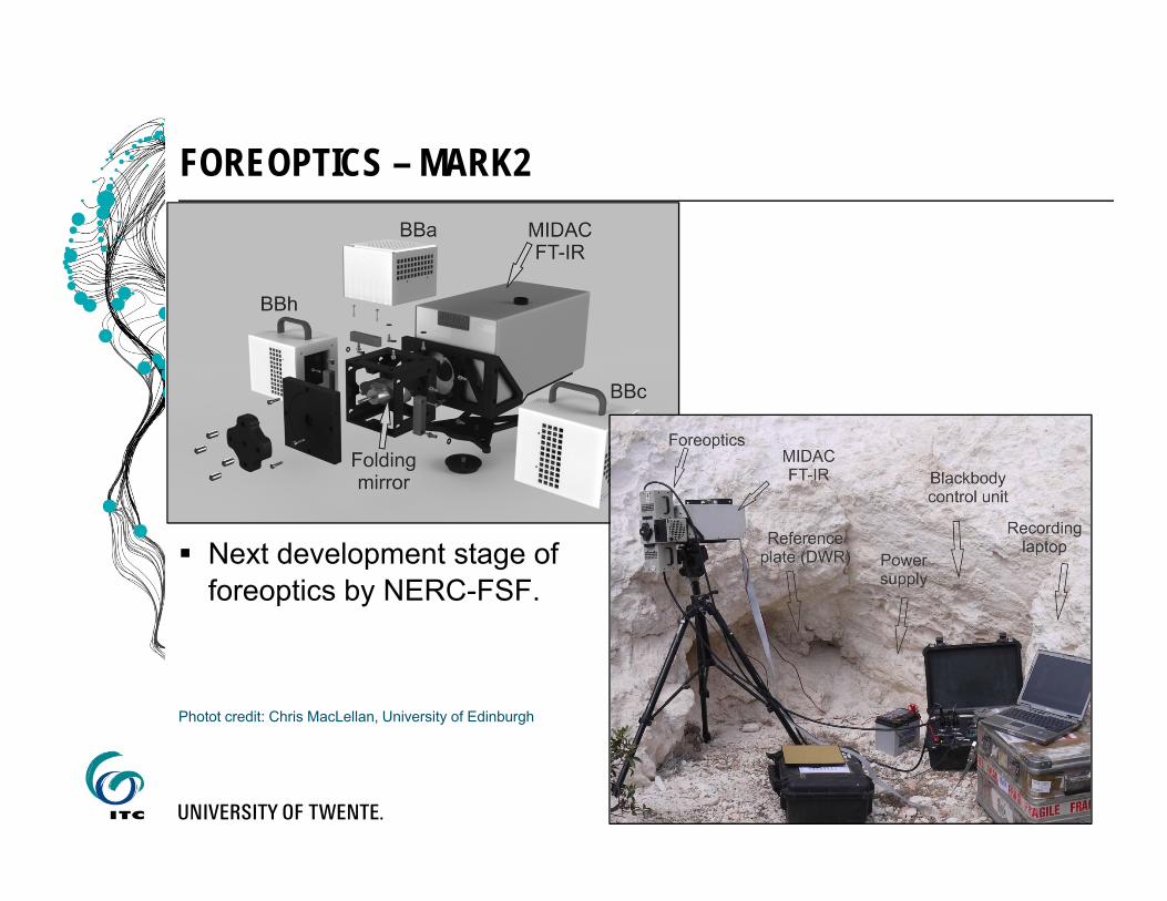
FOREOPTICS – MARK2

Next development stage of foreoptics by NERC-FSF.

Photot credit: Chris MacLellan, University of Edinburgh

FIELD IMAGING SPECTROMETER – TELOPS HYPERCAM

Emissive system Imaging FTIR Spectral range: 7.7 - 11.5 µm Image pixels: 320 x 256 Calibration: 2 Blackbodies Weight: ~30 Kg

AGILENT EXOSCAN 4100

Diffuse reflectance measurements

Not quantitatively comparable to emissive systems

Lightweight: ~3 Kg Comparable in use

to PXRF

CONSIDERATIONS - LABORATORY

Decide: speed or absolute emissivity values? Speed: bi-directional (cheap, fast, high SNR) Abs. Emiss: more effort, costs, measurement time

Abs. Emissivity: Sphere: long measurements, costs (1kEUR per cm

diameter) Emission: sample temperature control!

CONSIDERATIONS - FIELD

TIR field instruments not in ASD-like category

Decide: 50 kg equipment to field or 50 kg samples to lab?

Personal take on this question: Bring samples to lab except: Calibration Airborne campaigns Vegetation (?Lichen) Extremely large samples (e.g. entire quarry wall) Undisturbed soils and evaporite crusts

(sometimes sample rings possible?)

OUTLINE OF LECTURE

SWIR vs TIR Emissivity spectra of Minerals and Rocks Ground-based setups Laboratory Field Mapping methods Case study: TIR+PLSR

MAPPING METHODS

TIR preprocessing fundamentally different (e.g. TεS) After reduction to ground leaving radiance, same hyperspectral

tools as VNIR-SWIR mineral mapping, e.g.: Linear unmixing Partial Least Squares Regression (PLSR) Mixture Tuned Match Filter (MTMF) Spectral Angle Mapper (SAM) Feature fitting … etc.

OUTLINE OF LECTURE

SWIR vs TIR Emissivity spectra of Minerals and Rocks Ground-based setups Laboratory Field Mapping methods Case study: TIR+PLSR

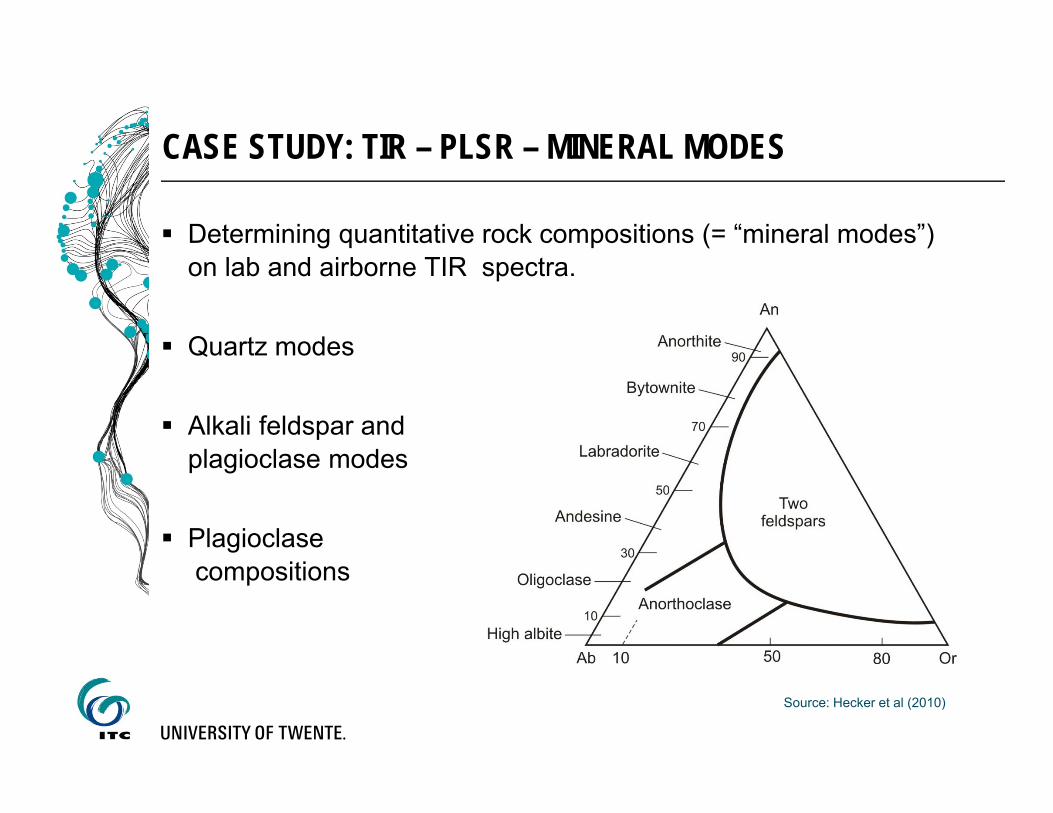
CASE STUDY: TIR – PLSR – MINERAL MODES

Determining quantitative rock compositions (= “mineral modes”) on lab and airborne TIR spectra.

Quartz modes

Alkali feldspar andplagioclase modes

Plagioclasecompositions

Source: Hecker et al (2010)

QUANTITATIVE TIR SPECTROSCOPYLINKING SPECTRA TO MINERALOGY AND MINERAL CHEMISTRY

sampleloclithunit_shpfile TS_name_long samplenr lithunit_Tssheet alteration quartz plagioclase kfsp diopside clinozoisite garnet plagcomp Bt_ign Bt_2nd Bt_total

563Jmd Y653_90067_26 Y‐563 QMD pervasive S‐2 or ES‐2 17 70 0 8 1tr 35 0 0 0653Jqmp Y653 Y‐653 QMP wk ab‐chl 3 19 4 0 0 0? 0.5 2 2.5

651Jmd2 y651_16_891 Y‐651 Jqmd ? 5 50 16 0 0 0strongly zoned 0 0 10

48Jqmp y48_90067_5 Y‐48 GP dike oli chl rt ep (py) 24 25 24 0 0 0 24 0 0 0787Jbqm y787_11_728 Y‐787 ?Jpqmj wk clay 30 35 27 0 0 0 25 0 0 5

692b Jqmp y692b Y‐692B ? wk sericitic 32 27 36 0 0 0 8 0.5 0 0.5681Jqmp y681_40_237 Y‐681 Jqmp wk potassic 5 21 7 0 0 0? 0 1 1684Jqmp y684_41_237 Y‐684 Jqmp wk potassic/ ep+chl 0.5 8 0 0 0 0? tr 1 1.25685Jbqmt y685_18_891 Y‐685 Qz monzodiorite ? 20 35 28 0 0 0 22 0 0 5688Jqmp y688_19_891 Y‐688 QMP ? 3 30 3 0 0 0 33 0 0 0

690b Jbqmt y690b_42_237 Y‐690‐B Jbqmt wk chl‐py‐ser / superg clay 30 27 27 0 0 0? 0.25tr 0.25693a Jbqm y693a Y‐693A Jbqm ? Possibly chl‐ser 22 32 31 0 0 0 35 0.5tr 0.5

700Jbqmt y700_43_891 Y‐700

transitional phase of border qz monozonite wk Kfsp‐clay‐ep 35 20 33 0 0 0 29 1 0 1

708b Jmd y708b_50_237 Y‐708B Jqmd wk potassic 10 50 15 0 0 0? 0 10 10750Jpqm y750_LDU‐3_thk Y‐750 PG Luhr Hill fresh 25 35 25 0 0 0 17 6 1 7665Jmd y665 Y‐665 QMD wk SW 10 40 8 0 0 0 20 3 0 3689Jmd y689 Y‐689 QMD Na‐Ca 12 45 9 0 0 0 28 3 0 3

690a Jbqmt y690 Y‐690A QMD wk Na‐Ca 7 42 12 0 0 0? 0 0 0691a Jbqm y691a Y‐691A BG PA 30 22 32 0 0 0 24 6 0 6691b Jbqm y691b Y‐691B QMD wk PA 6 55 6 0 0 0 7 0 0 0

46Jqmp y46_90067_4 Y‐46 GP dike Phlogo‐Chl‐Ep 0.25 25 0 0 0 0 26 0 0 0320Jmd y320_90067_11 Y‐320 QMD Act / Ep 9 50 9 0 0 0 0tr 0tr321Jmd y321_90067_12 Y‐321 QMD wk ES 10 55 12 5 0 0 25 3 0 3323Jbqm y323a_90067_12 Y‐323A BG wk PA 29 26 29 0 0 0 24 8 0 8323Jbqm y323b_90067_14 Y‐323B Andesite Dike ? 1 65 0 0 0 0? 0 0tr

335blueHill y335_grinding_b Y‐335 ?Andesite; Arthesia? 0 65 0 0 0 0 10 0 0 0680b Jqmp y680b_13_237 Y‐680‐B Jqmp ? 1 24 0 0 0 0 29 0 0.25 0.25692d Jdqmt y692d_43_237 Y‐692D Jbqm(t) Qz‐Tm‐Ser 32 21 27 0 0 0 32 0.125 4.5 4.625

797Jmd y797_15_7 Y‐797 Artesia Fm wk Ep‐clay‐Ab 0 53 0 0 0 0

strongly zoned and several generations 0 0 0

Thin section blocks Bruker FTIR TIR spectra

Thin section descriptionTS descr. In Spreadsheet

QUANTITATIVE TIR SPECTROSCOPYLINKING SPECTRA TO MINERALOGY AND MINERAL CHEMISTRY

PLSRModel

Training spectra

Sample spectra

XRDXRF

SEMPThinsection

Reference methods

Predicted

mineralogy

and

mineral

chemistry

Mod

el T

rain

ing

Model Prediction

WHAT IS PLS?

Regression method Links attribute data to spectra Decomposes into components similar to Principal Component

Analysis Good for spectroscopy: Compresses info into a few components Can deal with lots of bands and selects the most important Deals well with correlated attributes (adjacent bands often 99%

correlated)

SIMPLIFIED PLS EXAMPLE

Model Building50% Ser30% Qtz20% Ser60% Qtz

Prediction??% Ser ??% Qtz

PLSR ON TIR SPECTROSCOPYPREDICTION RESULTS

Regression coefficients and meas. vs. predicted plot

K-spar content

Source: Hecker et al (2011)

PLSR ON TIR SPECTROSCOPYPREDICTION RESULTS

21/01/2011IAMG Workshop @ITC

Plag content

Quartz content

Plag composition

Source: Hecker et al (2011)

PLSR ON TIR SPECTROSCOPYPREDICTION RESULTS

Mineral Ksp Plg Qtz Plgcomp

Number of LV's used 5 4 2 5

RMSEP [in %abs] 5.13 8.52 6.90 7.79

R2 0.81 0.80 0.70 0.59

slope (of regression line) 0.86 0.82 0.79 0.61

PLSR ON TIR SPECTROSCOPYMODEL INTERPRETATION (CASE OF QUARTZ)

Component 1:dominated by quartz Component 2:dominated by lack of albite

Combination of Comp1 and Comp2

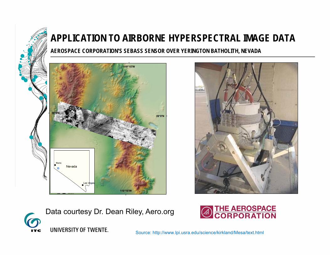
Source: http://www.lpi.usra.edu/science/kirkland/Mesa/text.html

Data courtesy Dr. Dean Riley, Aero.org

APPLICATION TO AIRBORNE HYPERSPECTRAL IMAGE DATAAEROSPACE CORPORATION’S SEBASS SENSOR OVER YERINGTON BATHOLITH, NEVADA

62

YERINGTON FIELD IMPRESSIONS

MacArthur Mine (porphyry Cu)

Yerington Mine (porphyry Cu)

SEBASS d-stretched Colour Composite

63

YERINGTON FIELD IMPRESSIONS (CONT’D)

Breccia with Cu-Oxides

Granite w/ Epidoteand Hornblende

MODELING FIRST

Adding noise up to 1% (absolute) to emissivity spectra gives OK results

Source: Hecker (2012)

NORMALIZING SPECTRAL CONTRAST

Airborne spectra have minimal spectral contrast

For quantitative results, spectral contrast needed normalization.

Source: Hecker (2012)

AIRBORNE HYPERSPECTRAL IMAGINGYERINGTON TIR COLOUR COMPOSITE RGB = (11.1, 9.64, 9.06)

Tailings

Cu-Skarn

Epithermal Auadvanced argillic

Porphyry CuK-alteration

QUANTITATIVE AIRBORNE ANALYSISAPPLYING PLS MODEL TO AIRBORNE DATA – QTZ CONCENTRATION AS GRAYSCALE IMAGE

QUANTITATIVE AIRBORNE ANALYSISAPPLYING PLS MODEL TO AIRBORNE DATA – DENSITY SLICED

Quartz concentrations100 % Qz

50 % Qz0 % Qz

SOURCES OF ADDITIONAL INFORMATION: TEXTBOOKS WITH TIR CHAPTERS

C. Kuenzer und S. Dech (Eds.) Thermal Infrared Remote Sensing: Sensors, Method, Applications (2013)

Drury (2001): Image Interpretation in Geology (3rd Edition); Chapter 6

Lillesand & Kiefer (2000): Remote Sensing and Image Interpretation (4th Edition); Chapter 5

Sabins (1997): Remote Sensing – Principles and Interpretation (3rd Edition); Chapter 5

Abrams et al (2001): Imaging Spectrometry in the Thermal Infrared; in vanderMeer & de Jong (2001): Imaging Spectrometry; Chapter 10

The Remote Sensing Tutorialhttp://www.fas.org/irp/imint/docs/rst/Section 9

Gupta (2003): Remote Sensing Geology (2nd Edition); Chapter 9

SOURCES OF ADDITIONAL INFORMATION: ARTICLES AND CHAPTERS MENTIONED IN TEXT

Hecker et al. (2013) Thermal Infrared Spectroscopy in the Laboratory and Field in Support of Land

Surface Remote Sensing. http://dx.doi.org/10.1007/978-94-007-6639-6_3

Riley and Hecker (2013) Mineral Mapping with Airborne Hyperspectral Thermal Infrared Remote

Sensing at Cuprite, Nevada, USA, http://dx.doi.org/10.1007/978-94-007-6639-6_24

van der Meer et al. (2012) Multi - and hyperspectral geologic remote sensing : a review.

http://dx.doi.org/10.1016/j.jag.2011.08.002

Hecker et al. (2012) Thermal infrared spectroscopy and partial least squares regression to determine

mineral modes of granitoid rocks. http://dx.doi.org/10.1029/2011GC004004

Hecker et al. (2011) Thermal infrared spectrometer for earth science remote sensing applications :

instrument modifications and measurement procedures. http://dx.doi.org/10.3390/s111110981

Hecker et al. (2010) Thermal infrared spectroscopy on feldspars : successes, limitations and their

implications for remote sensing. http://dx.doi.org/10.1016/j.earscirev.2010.07.005

QUESTIONS??