Embed Size (px)
Citation preview

Infrared QCD resummations at hadron colliders
A thesis submitted to the University of Manchester for the degree of
Doctor of Philosophy in the Faculty of Engineering and Physical Sciences
2011
Rosa Marıa Duran Delgado
Particle Physics Group
School of Physics and Astronomy

Contents
1 Introduction 6
1.1 The Standard Model . . . . . . . . . . . . . . . . . . . . . . . . . . 7
1.2 QCD in a nutshell . . . . . . . . . . . . . . . . . . . . . . . . . . . . 8
1.3 The QCD Lagrangian . . . . . . . . . . . . . . . . . . . . . . . . . . 9
1.4 Hadronic cross-sections and factorization . . . . . . . . . . . . . . . 12
1.5 Our research . . . . . . . . . . . . . . . . . . . . . . . . . . . . . . . 14
2 Novel aT variable for the study of Z boson production 16
2.1 Z-boson production at hadron colliders . . . . . . . . . . . . . . . . 16
2.2 Non-perturbative or “intrinsic” kT . . . . . . . . . . . . . . . . . . . 17
2.3 The novel aT observable . . . . . . . . . . . . . . . . . . . . . . . . 19
2.4 Definition of aT and soft limit kinematics . . . . . . . . . . . . . . . 22
2.5 Born cross-section . . . . . . . . . . . . . . . . . . . . . . . . . . . . 25
2.6 Leading Order distribution . . . . . . . . . . . . . . . . . . . . . . . 29
2.6.1 LO matrix elements . . . . . . . . . . . . . . . . . . . . . . . 30
2.6.2 Integration over three-body phase-space . . . . . . . . . . . 32
2.6.3 Logarithmic singularities in the aT distribution . . . . . . . 37
2.7 Resummation of large logarithms in aT . . . . . . . . . . . . . . . . 42
2.7.1 The resummed exponent . . . . . . . . . . . . . . . . . . . . 46
1

2.8 Comparison to fixed-order results . . . . . . . . . . . . . . . . . . . 52
2.9 Discussion and conclusions . . . . . . . . . . . . . . . . . . . . . . . 56
3 Gaps between jets at the LHC 60
3.1 Cross-section for dijet production . . . . . . . . . . . . . . . . . . . 64
3.2 Colour-basis independent notation . . . . . . . . . . . . . . . . . . . 66
3.2.1 Soft gluon emission . . . . . . . . . . . . . . . . . . . . . . . 67
3.2.2 Mapping onto a particular colour basis . . . . . . . . . . . . 70
3.3 The gap fraction . . . . . . . . . . . . . . . . . . . . . . . . . . . . 71
3.4 The resummed calculation . . . . . . . . . . . . . . . . . . . . . . . 73
3.4.1 Non-global contribution . . . . . . . . . . . . . . . . . . . . 75
3.5 Matching . . . . . . . . . . . . . . . . . . . . . . . . . . . . . . . . 78
3.5.1 Energy-momentum conservation . . . . . . . . . . . . . . . . 82
3.6 Matched results and comparison to data . . . . . . . . . . . . . . . 85
3.7 Discussion and conclusions . . . . . . . . . . . . . . . . . . . . . . . 89
Word count : 85690
2

Abstract
Infrared QCD resummations at hadron colliders
A thesis submitted to the University of Manchester
for the degree of Doctor of Philosophy
in the Faculty of Engineering and Physical Sciences
by Rosa Marıa Duran Delgado.
In this thesis we study two different processes at hadron colliders: Z-boson
production and dijet production with a jet veto. Our calculations focus on the
resummation of logarithmically enhanced contributions coming from soft and/or
collinear gluon emission.
For Z-boson production, we calculate the cross-section distribution in aT , a
novel variable proposed by Vesterinen and Wyatt as a more accurate probe of the
Z at low transverse momentum pT . The observable aT is defined as the component
of pT perpendicular to an experimentally convenient axis: the axis with respect to
which the two final-state leptons (from a Z leptonic decay) have equal transverse
momenta. Our study involves the resummation of large logarithms in aT /pT up to
next-to-leading accuracy. We then compare the resulting distributions in aT to the
well-known pT distribution, identifying important physical differences between the
two cases. We also test our resummed result at the two-loop level by comparing its
expansion with a fixed-order calculation and find agreement with our expectations.
Besides, we study dijet production with a veto in the inter-jet rapidity region
in proton-proton collisions. We resum the leading logarithms in the ratio of the
transverse momentum of the leading jets and the veto scale and we match this re-
sult to leading-order QCD matrix elements, taking into account energy-momentum
conservation effects. We compare our theoretical predictions to experimental data
measured by the ATLAS collaboration and find good agreement, although our
results are affected by large theoretical uncertainties.
3

Declaration
No portion of the work referred to in this thesis has been submitted in support of
an application for another degree or qualification of this or any other university or
other institute of learning.
Copyright statement
i. The author of this thesis (including any appendices and/or schedules to this
thesis) owns certain copyright or related rights in it (the Copyright) and she has
given The University of Manchester certain rights to use such Copyright, including
for administrative purposes.
ii. Copies of this thesis, either in full or in extracts and whether in hard or
electronic copy, may be made only in accordance with the Copyright, Designs
and Patents Act 1988 (as amended) and regulations issued under it or, where
appropriate, in accordance with licensing agreements which the University has
from time to time. This page must form part of any such copies made.
iii. The ownership of certain Copyright, patents, designs, trade marks and
other intellectual property (the Intellectual Property) and any reproductions of
copyright works in the thesis, for example graphs and tables (Reproductions),
which may be described in this thesis, may not be owned by the author and may
be owned by third parties. Such Intellectual Property and Reproductions cannot
and must not be made available for use without the prior written permission of
the owner(s) of the relevant Intellectual Property and/or Reproductions.
iv. Further information on the conditions under which disclosure, publication
and commercialisation of this thesis, the Copyright and any Intellectual Property
and/or Reproductions described in it may take place is available in the University
IP Policy, in any relevant Thesis restriction declarations deposited in the University
Library, The University Library’s regulations and in The University’s policy on
presentation of Theses.
4

Acknowledgments
First, I want to thank my supervisor Jeff Forshaw for his guidance, physics insights
and great support during my studies in Manchester. In these respects, I also
want to thank the rest of members of the Manchester HEP group for the many
interesting discussions we have as a joined theoretical and experimental team. In
particular, many thanks to Mrinal Dasgupta, Simone Marzani, Mike Seymour and
Fred Loebinger. I appreciate as well the financial support provided by the group.
Other physicists, not based in Manchester, have also helped me a great deal
in the understanding of QCD and the use of some computational tools for the
analysis of its phenomenology. Thanks to Andrea Banfi, in particular. Thanks
to the group of Theoretical High Energy Physics at Lund University for giving
me the motivation to continue doing research in the thrilling field of theoretical
Particle Physics.
Special thanks to Hector Silva and my family. Also to my friends (Silvia Pina,
Gabriel Pareyon, Jose Corrales, Paco Rıos, Jose Grima, Ana Marr, Marta Tavera,
Tim Coughlin, Ira Nasteva. . . ) that have broadened my views and helped me
countless times in these last few years. Gracias.
5

Chapter 1
Introduction
The largest particle accelerators currently operative in the world are the Large
Hadron Collider (LHC) at CERN, in Geneva, and the Tevatron at Fermilab, near
Chicago. Both of them are hadron colliders. The experimental data taken from
them will give us insight into the building blocks of reality as we perceive it. It will
provide information about the constituents of hadrons1, and the electromagnetic,
weak and strong interactions. In principle, one could derive analytical descriptions
of the physics phenomena observed at these high-energy scales. However, this can
only happen if we understand the ways in which the constituents of hadrons mesh
with each other. Thus, significant effort is currently devoted to improving the the-
ory of Quantum Chromo-Dynamics (QCD), the fundamental theory of the strong
force between point-like quarks, constituents of hadrons; and massless gluons, me-
diators of the force.
1Hadrons are protons and neutrons (components of atomic nuclei), and other particles that
can undergo strong interactions.
6

1.1 The Standard Model
The theory of QCD is included in the so-called Standard Model of Particle Physics,
which also describes electro-weak phenomena. The Standard Model is a dynamical
theory of relativistic and quantized fields, associated to a few particles, which
are assumed to be elementary; its Lagrangian manifests local invariance under
certain gauge transformations (see for example ref. [1] for a detailed description
of the theory).
Let me briefly explain the ideas that lead to the construction of the Stan-
dard Model. In the realms of Particle Physics we cannot neglect the effects that
occur at short distances and at high speeds. These counter-intuitive effects are de-
scribed by Quantum Mechanics and Special Relativity, so both theories are taken
into account in the Standard Model of Particle Physics. Besides, physics phe-
nomena always seem to manifest symmetries: some quantity remains unchanged
in any physical process. Symmetries thus constitute the core around which the
Standard Model is built.
The Lagrangian of the Standard Model arises almost naturally by following
these ideas. The resulting expression is rather condensed and elegant from a math-
ematical point of view, while at the same time it has proven to be very successful
at describing many observables at particle colliders. Perhaps even more interesting
is the fact that the theory includes, in its simple Lagrangian, physics from nuclear
and atomic scales, as well as the classic Maxwell equations of electromagnetism,
patent in our day-to-day experience.
Let us now introduce some key ideas of QCD, before describing our calculations.
7

1.2 QCD in a nutshell
In summary, QCD is a SU(3) non-Abelian gauge theory that has shown good
agreement with a large body of data taken mainly from particle colliders (see [2]
and references therein).
According to this theory, each quark (quarks are the constituents of hadrons)
takes one out of three possible charges, illustratively named colours, and always
manifests in nature combined with other quarks into colour-singlet states. This is
an important element of the theory, it is the property known as colour confinement.
QCD also embodies the idea that quarks behave as free particles in processes
involving short distance/time scales, associated with large momentum transfers.
Phenomena can be appropriately described in these realms through perturbative
techniques, like those used in the calculation of electromagnetic observables from
the simpler gauge-field theory of Quantum Electrodynamics. This second property
is known as asymptotic freedom.
The quantum field theory of QCD is capable of explaining this rather strange
behaviour of the strong interaction. The properties of asymptotic freedom and
quark confinement can be inferred from the dynamic content of the theory, i.e.
from its Lagrangian, which will be reviewed in next section.
Let us now see how QCD describes the dependence of the strong coupling on
the energy of a scattering event. The quantum-field theory of QCD needs to be
renormalized if one wants to get rid of unphysical ultraviolet divergences. In this
renormalization procedure we need to introduce an arbitrary mass scale, known as
a renormalization scale. Since physical observables (calculated in a perturbation
series of the coupling αs = g2/4π) cannot depend on this scale, the renormalized
running coupling must include some dependence on the cut-off scale (see the details
8

in Ref. [2]).
The dependence of the strong coupling αs = g2/4π on the renormalization scale
Q2 is given by
dαs
d ln Q2= β
(αs(Q
2))
= −αs(Q2)[β0αs(Q
2) + β1α2s(Q
2) + . . .]
(1.1)
where the beta function coefficients are defined as [2]
β0 =11CA − 2nf
12π, β1 =
17C2A − 5CAnf − 3CF nf
24π2, (1.2)
nf being the number of active quark flavours, CF = 4/3 the colour factor associated
with gluon emission from a quark and CA = 3 the colour factor associated with
gluon emission from a gluon.
The two-loop coupling equation (used throughout this thesis), running from
energy scale M2 to Q2, is given by
αs(Q2) =
αs(M2)
1− ρ
[1− αs(M
2)β1
β0
ln(1− ρ)
1− ρ
], ρ = αs(M
2)β0 lnM2
Q2. (1.3)
We see that the coupling increases at decreasing scales and gets weaker as the
momentum increases. The rate of decrease of αs is slow though (falling as ln−1 Q2)
and one often needs to include corrections to leading order perturbative results.
Moreover, as the coupling becomes large at small scales, perturbation theory is
no longer valid and one needs non-perturbative input, for example the so-called
parton-distribution functions, as we will see in section 1.4.
1.3 The QCD Lagrangian
The perturbative QCD Lagrangian density is given by
LQCD =∑
flavours
q(x)(iγµDµ−m) q(x)− 1
2Tr[Fµν(x)F µν(x)] +LGF +Lghost . (1.4)
9

Hereafter we will neglect the contributions of the gauge fixing LGF and ghosts
Lghost terms; they are introduced to properly quantize the theory, but the details
are beyond the scope of this thesis.
The first term (a sum over quark flavours) gives rise to the usual Dirac equation
for the quarks. We represent each quark by q(x), an N-tuplet of relativistic fermion
fields, where N is the number of colours N ≡ Nc = 3. The components of the
N-tuplet represent different states of the quark, all of them having the same mass
m, but different colours.
The dynamics of the spin-1 gluon fields is given by the second term
− 1
2Tr[Fµν(x)F µν(x)] . (1.5)
Like in the electromagnetic theory, we define the field strength tensor F in terms
of the gauge field, as
Fλρ(x) = DλGρ(x)−DρGλ(x) . (1.6)
In QCD the gauge field is the colour-octet field of the gluon Gµ(x) = Gaµ(x)ta.
It contains the gluon four-potentials, Gaλ(x), a = 1, . . . 8. ta represents the colour
charge. The properties of the colour matrices ta ≡ λa/2 are important in what
follows, so we summarize them:
[λa/2, λb/2] = ifabcλc/2 , (1.7)
fabc are totally antisymmetric in a, b, c, and are called the structure constants.
Equation (1.7) defines the Lie algebra of the group. The normalization is usually
chosen so that Tr(λaλb) = 2δab. Then the colour matrices satisfy the following
relations: ∑a
tija tjka = CF δik , CF =N2 − 1
2N=
4
3, (1.8)
10

∑a,b
fabc fabd = CA δcd , CA = N = 3 . (1.9)
Equation (1.4) is obtained from the requirement of gauge invariance of the
theory. The Lagrangian needs to be invariant under the following transformations
of the quark and gauge fields respectively:
q(x) → U(x)q(x) (1.10)
Fµν → UFµνU† , (1.11)
with
U(x) = eiωa(x)ta . (1.12)
U(x) is a N ×N matrix, hermitian and traceless, which must include the identity
matrix; in other words, U(x) ∈ SU(3). Thus, the invariant transformation of the
fermion field is just a SU(Nc) rotation through ω, the colour matrices ta being the
N2c − 1 generators of the rotation.
Note that the requirement of gauge invariance of the Lagrangian implies that
the operator Dµ cannot simply be the usual covariant derivative ∂µ. Dµ is instead
given by
Dµ = 1 ∂µ + i gsGµ(x) , (1.13)
where gs is the dimensionless strong coupling constant. This is the minimal sub-
stitution of the derivative operator that guarantees gauge invariance. Inserting
Dµ in Eq. (1.6) and then into the Lagrangian, we find explicitly the terms that
describe the triplet and quartic gluon self-interactions. These ‘non-Abelian’ terms
are ultimately responsible for the property of asymptotic freedom.
Likewise, the term −gs q γµ Gaµ taq is implicit in the Lagrangian with the def-
inition of Dµ in expression (1.13). This term describes the ‘minimal interaction’
11

between gluons and quarks. The interaction between one gluon and two quarks is
thus explained in the theory as a mere consequence of gauge invariance.
1.4 Hadronic cross-sections and factorization
The formula that we will use to calculate hadronic cross-sections is the following:
dσh1h2→X =∑i,j
∫ 1
0
∫ 1
0
fi(x1, µ2) fj(x2, µ
2) dσij→X(Q2/µ2) dx1dx2 . (1.14)
We consider the hard scattering as if it was simply initiated by any two partons
(quarks or gluons) of type i, j. The parton distribution functions (pdfs) fi(x, µ2)
are the number densities of partons of type i carrying a fraction x of the longitudi-
nal momentum of the incoming hadrons, when resolved at a factorization scale µ,
and dσij→X are the partonic contributions to the cross-section. The pdfs include
in their definition the emission of quarks and gluons from the original partons
when they are emitted with some transverse momentum below the factorization
scale; this is known as initial-state collinear radiation. The factorization scale is an
arbitrary parameter that we set to separate long- and short-distance components
of the cross section; practically speaking it should be chosen of the order of the
hard scale that characterizes the process. The pdfs are universal (independent of
the type of scattering but dependent on the type of incoming particle) and they
have values taken from experiment. Their evolution in terms of the scale µ2 can
be calculated perturbatively through the DGLAP equations [3–6].
If the cross-section is defined in terms of final-state hadrons then one also needs
to convolute the partonic cross-sections with fragmentation functions, to include
the effects of hadronization. We will not be considering such observables in this
thesis.
12

dσ Collinear gluon → fi(x, µ2)
Soft gluon
Figure 1.1: Typical QCD event with a hard partonic interaction marked in red, initial-
state gluon collinear emission in blue and soft gluon virtual radiation illustrated in green.
Hence we see explicitly a factorization of long and short distance physics in
Eq.(1.14). The factorization theorem expresses the idea that the soft colour field
generated by the incoming hadrons does not affect the probability for the hard
collision. However, at each order in the perturbative series of our QCD calculations
large logarithmic terms arise from gluons whose momentum components are all
small compared with the scale of the scattering [8]. These soft gluons cannot
generally be factorized into the pdfs; instead they are calculated as corrections to
the primary hard scattering and they are included in dσ. In our body of work we
will study the impact of soft gluon emission on the cross-sections of two different
hadronic-scattering scenarios, Z-boson production and gaps between jets.
13

1.5 Our research
In this thesis we focus on two particular scenarios that can give us insight in the
understanding of the infrared sector of QCD: Z-boson production, via the channel
hh → Z → ll, and dijet events with a jet veto within the rapidity interval between
the two jets.
In the former type of event, the kinematics of the produced Z boson can be pre-
cisely determined from its particular clean decay to a pair of charged leptons. In
the spectrum of its transverse momentum pT , specifically at low values, we find con-
tributions coming from non-perturbative QCD radiation. These non-perturbative
effects are universal and therefore expected to be present also in events involv-
ing new physics, such as the production of SUSY particles or the Higgs boson.
However, this region of the pT distribution is highly sensitive to experimental sys-
tematics, and the data available are not yet precise enough to accurately constrain
the modeling of the non-perturbative effects. In this context, we provide the first
theoretical study of a novel variable aT , proposed in Ref. [9] as a more accurate
probe of the region of low transverse momentum pT . Our calculation of the aT dis-
tribution for Z-boson production at hadron colliders (which involves resummation
of large logarithms in aT ) will be presented in Chapter 2.
The second process that we study can also give us much information on the role
of soft gluons in QCD: it is dijet production in proton-proton collisions with a veto
on the emission of a third jet in the rapidity region in between the two leading
ones. In Chapter 3, we explain our calculation for its cross-section. In short,
we make a soft-gluon resummation of the most important logarithms in the ratio
of the transverse momentum of the leading jets and the veto scale. We include
leading logarithms and a (partial) tower of non-global logarithms coming from the
14

emission of one gluon outside the gap. Then we match this result to leading-order
QCD matrix elements. We find that, in order to obtain sensible results, we have
to modify the resummation and take into account energy-momentum conservation
effects. We compare our theoretical predictions for the gap fraction to experimental
data measured by the ATLAS collaboration and find good agreement, although our
results are affected by large theoretical uncertainties. We then discuss differences
and similarities of our calculation to other theoretical approaches.
15

Chapter 2
Novel aT variable for the study of
Z boson production
2.1 Z-boson production at hadron colliders
The production of W and Z bosons at hadron colliders via the Drell-Yan process [2]
has formed a very significant part of particle phenomenology almost since their
discovery [10–12]. In the era of the LHC these studies continue to occupy an
important role for a variety of reasons. For instance, an accurate understanding of
the production rates and pT distributions of the W and Z can be used for diverse
purposes which range from more prosaic applications such as luminosity monitoring
at the LHC to measurement of the W mass and perhaps most interestingly for
discovery of new physics, which may manifest itself via the decay of new gauge
bosons to lepton pairs.
In particular, the pT spectrum of the Z/γ∗ bosons (denoted simply as “Z
bosons” throughout this thesis) has received considerable theoretical and experi-
mental attention in the past, but there remain aspects where it is desirable to have
16

an improved understanding of certain physical issues. One such important issue
is the role of the non-perturbative or “intrinsic” kT component (explained in the
following section) which may have a sizable effect on the pT spectrum at low pT
(see e.g Refs. [13–15]).
For the precise determination of pT spectra at the LHC, it is important to have
as thorough a probe of the low pT region of Z-boson production as it is possible.
Investigations carried out using the conventional pT spectrum mainly suffer from
large uncertainties arising from experimental systematics, dominated by resolution
unfolding and the dependence on pT of event selection efficiencies, as represented
in Fig. 2.1 and discussed in detail in Ref. [9].
2.2 Non-perturbative or “intrinsic” kT
The incoming quarks/anti-quarks which partake in any event at the Tevatron or
LHC hadron colliders are part of extended objects (protons or anti-protons) and
have interactions with other constituents thereby generating a small transverse
momentum kT . This transverse momentum can be viewed as the Fermi motion of
partons inside the proton and a priori one might expect it to be of order of the
QCD scale ΛQCD.
Since the intrinsic kT has a non-perturbative origin it cannot be computed
within conventional methods of perturbative QCD. One can however model the
intrinsic kT as an essentially Gaussian smearing of the perturbatively calculated
pT spectra and hope to constrain the parameters of the Gaussian by fitting the
theoretical prediction to experimental data. An example of this procedure is pro-
vided by the work of Brock, Landry, Nadolsky and Yuan (BLNY). Their proposed
non-perturbative Gaussian form factor in conjunction with perturbative calcula-
17

)-1(G
eVTQ/
! d
!1/ 0.02
0.040.060.08
0.10.120.14
(no cuts)genX
(all cuts)detX
(d)
(GeV)TQ
0 5 10 15 20 25 30
gen
X)/gen
-Xdet
X(
-0.6-0.4-0.2
00.20.40.6
)-1(G
eVTa/
! d
!1/
0.020.040.060.08
0.10.120.140.16
(no cuts)genX
(all cuts)detX
(a)
(GeV)Ta0 2 4 6 8 10 12 14 16 18 20
gen
X)/gen
-Xdet
X( -0.06-0.04-0.02
00.020.040.06
Figure 2.1: Monte Carlo simulations of the generator and detector level distributions
at the Run II D∅ detector for (left) the Z boson transverse momentum pT and (right)
the novel variable aT described in next section. The detector level distributions are
for Gaussian smearing in 1/QT ≡ 1/pT of width 0.003 GeV−1 (which simulates the
imperfect lepton pT resolution of the detector), and all selection cuts are applied. The
generator level distributions do not include selection cuts. The lower halves of each plot
show the fractional differences. Figures from Ref. [9].
18

tions was able to describe both Tevatron Run-1 Z data as well as Drell-Yan data
corresponding to lower scattering energies [15]. Alternatively to this procedure,
one may also use a Monte Carlo event generator such as HERWIG++ [16] to inves-
tigate this issue. As discussed in Ref. [17] these studies yield kT values somewhat
larger than expected and also reveal a dependence of this quantity on the collider
energy, which features are desirable to understand better.
Additionally, as pointed out by Berge et al. [18], studies from semi-inclusive DIS
events at the HERA-ep collider suggest a small-x broadening of their form factor,
for small Bjorken-x values (x < 10−3).1 Extrapolating the effect to the LHC
where such small-x values become relevant, one may expect to see significantly
broader Higgs and vector boson pT spectra than one would in the absence of
small-x effects [18]. Berge et al. suggested that Tevatron studies with samples of
vector-boson with high rapidities would help to provide further information on the
role, if any, of the small-x broadening on non-perturbative parameters. The D∅
Run II data on pT [20] was not particularly sensitive to such broadening at low pT
(see Fig. 2.2) and more precision is required to reach any conclusion.
2.3 The novel aT observable
We have seen that the low values of pT of Z bosons produced at hadron col-
liders form a distribution particularly interesting for the understanding of non-
perturbative effects. However, the measured pT is highly sensitive to experimental
systematics, in particular to the transverse-momentum resolution of the leptons
1This x dependence may be merely an effective parametrisation of missing perturbative BFKL
effects. Another observable was suggested in Ref. [19] to investigate this x dependence: the pT -
component in one hemisphere in the DIS Breit frame.
19

(GeV/c)T
* q!Z/0 5 10 15 20 25 30
-1 (G
eV/c
)T
/dq
" d×
"1/
0.02
0.04
0.06
0.08
0.1|y|>2
ResBos with small-x effectResBos without small-x effectDØ data
DØ, 0.98 fb-1
(b)
Figure 2.2: Normalized Z boson transverse momentum distributions. The points are
the D0 Run II data, the solid curve is the ResBos prediction and the dashed line is the
prediction from the form factor modified after studies of small-x DIS data. ResBos [21]
is an event generator which incorporates a resummation at all perturbative orders for
low pT , including the BLNY non-perturbative form factor, and then matches it to a
fixed order NLO perturbative calculation for high pT . Figure published in Ref. [20].
produced by the Z boson and also to the overall event selection efficiency.
An alternative observable to study the low Z pT region should ideally be less
sensitive to experimental systematic errors, whilst still sensitive to the Z boson pT .
Keeping in mind that collider detectors generally have far better angular resolution
than calorimeter transverse momentum track resolution, an observable satisfying
both of these requirements was proposed in Ref. [9]. This variable, aT , is defined
as the transverse component with respect to the lepton thrust axis. From Fig. 2.1
(published in Ref. [9]) it is clear that aT is experimentally better determined at
low values than the standard pT variable and hence it would make a more accurate
20
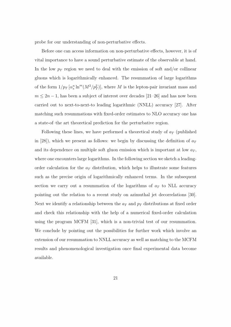
probe for our understanding of non-perturbative effects.
Before one can access information on non-perturbative effects, however, it is of
vital importance to have a sound perturbative estimate of the observable at hand.
In the low pT region we need to deal with the emission of soft and/or collinear
gluons which is logarithmically enhanced. The resummation of large logarithms
of the form 1/pT [αns lnm(M2/p2
T )], where M is the lepton-pair invariant mass and
m ≤ 2n− 1, has been a subject of interest over decades [21–26] and has now been
carried out to next-to-next-to leading logarithmic (NNLL) accuracy [27]. After
matching such resummations with fixed-order estimates to NLO accuracy one has
a state-of–the art theoretical prediction for the perturbative region.
Following these lines, we have performed a theoretical study of aT (published
in [28]), which we present as follows: we begin by discussing the definition of aT
and its dependence on multiple soft gluon emission which is important at low aT ,
where one encounters large logarithms. In the following section we sketch a leading-
order calculation for the aT distribution, which helps to illustrate some features
such as the precise origin of logarithmically enhanced terms. In the subsequent
section we carry out a resummation of the logarithms of aT to NLL accuracy
pointing out the relation to a recent study on azimuthal jet decorrelations [30].
Next we identify a relationship between the aT and pT distributions at fixed order
and check this relationship with the help of a numerical fixed-order calculation
using the program MCFM [31], which is a non-trivial test of our resummation.
We conclude by pointing out the possibilities for further work which involve an
extension of our resummation to NNLL accuracy as well as matching to the MCFM
results and phenomenological investigation once final experimental data become
available.
21

2.4 Definition of aT and soft limit kinematics
We are concerned in this chapter with large logarithms in the perturbative de-
scription of the aT variable and their resummation. Since these logarithms have
their origin in multiple soft and/or collinear emissions from the incoming hard
partons we need to derive the dependence of aT on such emissions. In this section
therefore we define aT and obtain its dependence on the small transverse momenta
kt of emissions.
We are considering the production of Z bosons via the Drell-Yan (and QCD
Compton) mechanisms which subsequently decay to a lepton pair. The aT is the
component of the lepton pair (or equivalently Z boson) pT transverse to a suitably
defined axis, sketched in Fig.2.3. The precise definition of the lepton thrust axis
Figure 2.3: Schematic representation in the transverse plane, of the novel aT observable,
where QT in the figure represents the standard transverse momentum pT of a Z boson
decaying leptonically. Figure from Ref. [9].
as employed in Ref. [9] is provided below:
n =~pt1 − ~pt2
|~pt1 − ~pt2|, (2.1)
where ~pt1 and ~pt2 are the transverse momenta of the two leptons and thus n is a
unit vector in the plane transverse to the beam direction. It is straightforward
22

to verify that this is the axis with respect to which the two leptons have equal
transverse momenta.
We now consider multiple emissions from the incoming partons which (neglect-
ing the intrinsic kT ) are back-to–back along the beam direction. From conservation
of transverse momentum we have ~pt1 + ~pt2 = −∑
i~kti which means that the lep-
ton pair or Z boson pT is just minus the vector sum of emitted gluon transverse
momenta ~kti, where we refer to the momentum transverse to the beam axis. To
obtain the dependence of aT on the kti we wish to find the component of this sum
normal to the axis defined in eq. (2.1). The axis is given by (writing ~pt2 in terms
of ~pt1 and ~kti)
n =2~pt1 +
∑i~kti
|2~pt1 +∑
i~kti|
≈ ~pt1
|~pt1|, (2.2)
where to obtain the last equation we have neglected the dependence of the axis on
emissions kti. The reason for doing so is that we are projecting the vector sum of
the kti along and normal to the axis and any term O (kti) in the definition of the
axis impacts the projected quantity only at the level of terms bilinear or quadratic
in the small kti. Such terms can be ignored compared to the leading linear terms
∼ kti that we shall retain and thus to our accuracy the axis is along the lepton
direction.2
We can parametrise the lepton and gluon momenta in the plane transverse to
the beam as below:
~pt1 = pt (1, 0)
~kti = kti (cos φi, sin φi) ,(2.3)
2To be more precise the recoil of the axis against soft emissions, if retained, corrects our result
only by terms that vanish as aT → 0. Such terms are beyond the scope of NLL resummation
but will be included up to NLO due to the matching.
23

where φi denotes the angle made by the ith emission with respect to the direction
of lepton 1 in the transverse plane. It is thus clear that, expressed in these terms,
the transverse component of the Z boson pT is simply −∑
i kti sin φi3 and one has
aT =
∣∣∣∣∣∑i
kti sin φi
∣∣∣∣∣ . (2.4)
We note immediately that the dependence on soft emissions is identical to the
case of azimuthal angle ∆φ between final state dijets near the back-to–back region
∆φ ≈ π, for which resummation was carried out in Ref. [30]. This is not surprising
since the component of the Z boson pT , transverse to the axis defined above, is
proportional in the soft limit to π − ∆φ, where ∆φ is the angle between the
leptons in the plane transverse to the beam. The other (longitudinal) component
of Z boson pT , aL, is proportional to pt1 − pt2 the difference in lepton squared
transverse momenta.4 Since it is possible to measure more accurately the lepton
angular separation compared to their pt imbalance (where momentum resolution
is an issue), one can obtain more accurate measurements of aT as compared to
aL or the Z boson pT which is given by√
a2T + a2
L [9]. The resummation that we
carry out in next section will be similar in several details to those of Refs. [30,32]
but simpler since the final state hard particles are colourless leptons.
In the following sections we shall study the integrated cross-section which is
directly related to the number of events below some fixed value of aT
Σ(aT , M2) =
∫ aT
0
d2σ
da′T dM2da′T , (2.5)
3The resummation for the variable ET =∑
i kti was performed in [29].4For the case of dijet production the leptonic pt imbalance has also been addressed via re-
summation in Ref. [32] which to our knowledge is the first extension of the pT resummation
formalism to observables involving final state jets.
24

from which the distribution in aT can be obtained by differentiation and the de-
pendence of Σ on M2 will be henceforth implied. We shall first review the Born
cross-section of the Drell-Yan process, which needs to be included in the total
cross-section defined in eq. (2.5). We will also compute the single and double loga-
rithmically enhanced terms in aT and relate them to the corresponding logarithms
in the standard pT distribution at leading order in αs. The discussion here should
facilitate an understanding of the resummation we carry out in the next section
and the results of subsequent sections.
2.5 Born cross-section
At Born level we have to consider the Drell-Yan process p1 + p2 = l1 + l2 where
p1, p2 and l1, l2 are the four momenta of incoming partons and outgoing leptons
respectively, the lepton pair being produced via Z decay. At this level the pT of
the lepton pair and hence aT vanishes, so that the full Born result, evaluated at
fixed mass M2, contributes to the cross-section in Eq. (2.5).
The Born cross section can be calculated from the following equation:
Σ(0)(M2) =
∫ 1
0
dx1
∫ 1
0
dx2 [fq(x1)fq(x2) + q ↔ q]×
×∫
dΦ(l1, l2)M2DY(l1, l2) δ
(M2 − 2 l1.l2
), (2.6)
where x1 and x2 are momentum fractions carried by partons p1 and p2 of the
parent hadron momenta, fq(x1) and fq(x2) denote parton distribution functions5,
dΦ(l1, l2) is the two-body phase-space, and M2DY is the Born matrix element given
5In order to avoid excessive notation we do not explicitly indicate the sum over incoming
parton flavours which should be understood.
25

by [33]
M2DY(l1, l2) =
8
Nc
G(α, θW , M2, M2
Z
) [Al Aq (t21 + t22) + Bl Bq (t21 − t22)
]. (2.7)
The electroweak coefficient constants G, Al, Aq, Bl, Bq for the case of Z boson
exchange are:
G(α, θW , M2, M2Z) =
4π2α2
sin4 θW cos4 θW
1
(M2 −M2Z)2 + (ΓZMZ)2
,
Af = a2f + b2
f , Bf = 2afbf , (f = l, q) .
(2.8)
All these quantities have been taken from Ref. [33], where the reader can find
analogous expressions for the case in which a virtual photon is exchanged as well.
Following the conventions of Ref. [33], we also have
al = −1
4+ sin2 θW , bl =
1
4,
au,c =1
4− 2
3sin2 θW , bu,c = −1
4,
ad,s,b = −1
4+
1
3sin2 θW , bd,s,b =
1
4.
(2.9)
Henceforth we shall suppress the dependence of G, which has dimension M−4, on
the standard electroweak parameters α, θW , MZ . The factor 1/Nc comes from the
average over initial state colours.
We have also defined the invariants6
t1 = −2p1.l1 t2 = −2p2.l1 , (2.10)
while M2 is the invariant mass of the lepton pair which we fix. The component
t21 + t22 is the parity conserving piece also present in the case of the virtual photon
6The quantities t1 and t2 were labeled as t1, t2 while l1 and l2 were labeled k1 and k2 in
Ref. [33].
26
process while the t21 − t22 component is related to the parity violating piece of the
electroweak coupling and hence absent for the photon case.
We now look at the Lorentz-invariant phase-space which can be written as∫dΦ(l1, l2) =
1
2s
∫d3l1
2(2π)3l10
d3l22(2π)3l20
(2π)4δ4(p1 + p2 − l1 − l2) , (2.11)
where s is the partonic centre of mass energy squared s = s x1x2. Note that in
addition to the usual two-body phase space we included a delta function corre-
sponding to holding the invariant mass of the lepton-pair at M2.
We parameterise the four vectors of the incoming partons and outgoing leptons
as below (in the lab frame)
p1 =
√s
2x1 (1, 0, 0, 1), (2.12)
p2 =
√s
2x2 (1, 0, 0,−1),
l1 = lT (cosh y, 1, 0, sinh y) ,
with l2 being fixed by the momentum conserving delta function.
In the above√
s denotes the centre of mass energy of the incoming hadrons,
while lT and y are the transverse momentum and rapidity of the lepton with respect
to the beam axis and we work in the limit of vanishing lepton and quark masses.
In these terms we can express Eq. (2.11) as (after integrating over l2 using the
momentum conserving delta function)∫dΦ(l1, l2) =
1
2s
∫lT dlT dy
4πδ((p1 + p2 − l1)
2)
, (2.13)
where we have carried out an irrelevant integration over lepton azimuth. Note that
the factor δ ((p1 + p2 − l1)2) arises from the vanishing invariant mass of lepton l2.
In order to obtain the full Born result we need to fold the above phase-space
with the parton distribution functions and the squared matrix element for the
27

Drell-Yan process to obtain
Σ(0)(M2) =
∫ 1
0
dx1 f(x1)
∫ 1
0
dx2 f(x2)×
× 1
2s
∫lT dlT dy
4πδ (s x1x2 + t1 + t2) δ
(M2 − x1x2s
)M2
DY, (2.14)
where we used (p1 + p2 − l1)2 = sx1x2 + t1 + t2.
We next evaluate the squared matrix element M2DY in Eq. (2.7) in terms of the
phase space integration variables, using:
t1 = −2p1.l1 = −√
s x1 lT e−y , t2 = −√
s x2 lT ey . (2.15)
Inserting these values of t1 and t2 in Eq. (2.14) we use the constraint
δ(s x1x2 + t1 + t2) = δ(s x1x2 −
√s lT
(x2 ey + x1 e−y
)), (2.16)
to carry out the integration over lT which gives
1
8πs
∫ 1
0
dx1 f(x1)
∫ 1
0
dx2 f(x2) δ(M2 − x1x2s
) dy
(x2ey + x1e−y)2 M2DY , (2.17)
where in evaluating M2DY one needs to use lT =
√s x1x2/(x2e
y + x1e−y) , which
yields using (2.15)
t21 = x21e−2y M4
(x2ey + x1e−y)2 , (2.18)
t22 = x22e
2y M4
(x2ey + x1e−y)2 .
Using the above to evaluate M2DY in (2.7) we obtain
Σ(0)(M2) =GNc
M4
πs
∫ 1
0
dx1 f(x1)
∫ 1
0
dx2 f(x2) δ(M2 − x1x2s
) ∫dyF(x1, x2, y),
(2.19)
where we introduced
F (x1, x2, y) = Al Aqx2
1e−2y + x2
2e2y
(x2ey + x1e−y)4 + Bl Bqx2
1e−2y − x2
2e2y
(x2ey + x1e−y)4 . (2.20)
28

Integrating the angular function F over rapidity over the full rapidity range7 one
finds as expected that the parity violating component proportional to Bl Bq van-
ishes and the result is Al Aq/(3x1x2). Thus the final result is (using x1x2 = M2/s)
Σ(0) ≡ Σ(0)(M2) =
= GM2
3π
Al Aq
Nc
∫ 1
0
dx1
∫ 1
0
dx2 [fq(x1)fq(x2) + q ↔ q] δ(M2 − sx1x2
). (2.21)
2.6 Leading Order distribution
We now derive the QCD corrections to leading order in αs with the aim of identi-
fying logarithmically enhanced terms in aT to the integrated cross-section defined
in Eq. (2.5). To this end we need to consider the process p1 + p2 = l1 + l2 + k
where k is a final state parton emission as well as O (αs) virtual corrections to the
Drell-Yan process.
Let us focus first on the real emission contribution. The processes to consider
are the emission of a gluon in the Drell-Yan (QCD annihilation) process as well
as the contribution of the quark-gluon (QCD Compton) scattering process. Thus
we consider the reaction p1 + p2 = l1 + l2 + k where k is the emitted gluon in the
Drell-Yan process and a quark/anti-quark for the Compton process. We need to
compute the quantity
Σ(1)(aT , M2) =
∫ 1
0
dx1
∫ 1
0
dx2
[fq(x1)fq(x2) + q ↔ q] Σ
(1)A (aT )
+ [(fq(x1) + fq(x1)) fg(x2) + q, q ↔ g] Σ(1)C (aT )
,
(2.22)
7We can straightforwardly adapt the calculation to include the experimental acceptance cuts
when available.
29

where the partonic quantities Σ(1)A/C which give the O(αs) contribution read
Σ(1)i (aT , M2) =
∫dΦ(l1, l2, k)M2
i (l1, l2, k)δ(M2 − 2l1.l2
)Θ (aT − kt| sin φ|) ,
(2.23)
where the index i runs over the contributing subprocesses at this order, i.e. i = A/C
denotes the annihilation (Drell-Yan)/Compton subprocesses while M2i is the ap-
propriate squared matrix element. We have introduced a delta function constraint
that indicates we are working at fixed invariant mass of the lepton pair 2l1.l2 = M2.
Additionally in order to compute the integrated aT cross-section Eq. (2.5), we need
to restrict the additional parton emission k such that we are studying events be-
low some value of aT . Recalling, from the previous section, that the value of this
quantity generated by a gluon with transverse momentum kt and angle with the
lepton axis φ is kt| sin φ| we arrive at the step function in the above equation.8 We
then fold the parton level result with parton distribution functions precisely as for
the Born level result Σ0 reported above.
2.6.1 LO matrix elements
The matrix element squared for the QCD annihilation process from Ref. [33] is (in
four dimensions)
M2A(l1, l2, k) = −16 g2 G CF
Nc
M2×
×
AlAq
[(1 +
s− 2t1 −M2
t− t21 + t22 + s (t1 + t2 + M2)
tu
)+(u ↔ t, t1 ↔ t2
)]+BlBq
[((s + 2t1 + M2)
t+
s (t1 − t2)
tu
)−(u ↔ t, t1 ↔ t2
)], (2.24)
8As we stated previously this approximation is sufficient up to terms that vanish as aT → 0,
which we do not compute here.
30

while for the QCD Compton process, if p2 represents an incoming gluon, one has
M2C(l1, l2, k) = −16 g2 G TR
Nc
M2×
×
AlAq
[t− 2 (t1 + M2)
s+
s + 2(t1 + t2)
t+
2
st
((t1 + t2 + M2
)2+ t21 − t2M
2)]
+BlBq
[2 (t1 + M2)− t
s+
s + 2 (t1 + t2)
t− 2M2 (2t1 + t2 + M2)
st
], (2.25)
where we corrected small errors (after an independent recomputation of the above)
of an apparent typographical nature in the BlBq piece of the annihilation result.
The kinematical variables u and t are the usual Mandelstam invariants
u = −2p1.k = −√
s x1 kt e−yk , t = −2p2.k = −
√s x2 kt e
yk , (2.26)
where we have explicitly parameterised the momentum k as below
k = kt (cosh yk, cos φ, sin φ, sinh yk) , (2.27)
the parameterisation of the other particles four-momenta being as in the Born case
Eq. (2.12).
In the limit of small rescaled transverse momentum ∆ = k2t /M
2 both matrix
elements become collinear singular. In the annihilation subprocess this occurs
when the emitted gluon k is collinear to either p1 (corresponding to u → 0) or
p2 (t → 0). The singularity for u → 0 occurs at positive gluon rapidity yk,
correspondingly the one for t → 0 occurs at negative yk. The matrix element for
the Compton process shows only a collinear divergence when an outgoing quark is
collinear to the incoming gluon, corresponding to t → 0.
In the following we compute the approximated expression of M2A and M2
C
in the collinear limit t → 0. The remaining collinear limit u → 0 of M2A gives
an identical result after integration over the lepton rapidity. Neglecting terms of
31
relative order kt one has
lT 'M2
√s (x1e−y + zx2ey)
, t ' − k2t
1− z, u ' −1− z
zM2 ,
t1 ' −x1e
−yM2
(x1e−y + zx2ey), t2 ' −
x2eyM2
(x1e−y + zx2ey), M2 ' −(t1 + z t2) ,
(2.28)
where 1− z is the fraction of the parent partons energy carried off by the radiated
parton. Substituting these expressions in Eq. (2.24) and Eq. (2.25) one obtains
M2A(l1, l2, k) ' 16 g2
z k2t
G CF
Nc
(1 + z2)[AlAq(t
21 + z2t22) + BlBq(t
21 − z2t22)
], (2.29)
and
M2C(l1, l2, k) ' 16 g2
z k2t
G TR
Nc
(1−z) [z2+(1−z)2][AlAq(t
21 + z2t22) + BlBq(t
21 − z2t22)
].
(2.30)
where the collinear singularity 1/k2t has been isolated. Note that the result is
proportional to the Born matrix element in Eq. (2.7) with x2 replaced by z x2,
indicating that the momentum fraction of the parton entering the hard scattering
has been reduced by a factor z after the emission of a collinear gluon.
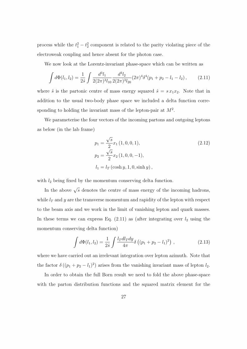
2.6.2 Integration over three-body phase-space
We now need to integrate the squared matrix elements over a three-body Lorentz
invariant phase-space Φ, since in addition to the final state lepton four-momenta
l1, l2 we also have a final state emitted parton k.
The Lorentz invariant phase-space is now∫dΦ(l1, l2, k) =
1
2s
∫d3l1
2(2π)3l10
d3l22(2π)3l20
d3k
2(2π)3k0
(2π)4δ4(p1 + p2 − l1 − l2 − k) .
(2.31)
Following the same procedure as in the Born case we perform the trivial integra-
tion over l2 and obtain the leading order QCD correction to the Born result (2.14)
32

(for the moment we are considering just real emission terms indicated below by
the label r)
Σ(1)r (M2) =
∑i=A,C
∫ 1
0
dx1 f(x1)
∫ 1
0
dx2 f(x2)×
× 1
2s
∫lT dlT dy
4π
d3k
2(2π)3k0
δ(M2 + t1 + t2 + 2l1.k
)×
× δ
(M2 − x1x2s
(1− 2p1.k
s− 2p2.k
s
))M2
i . (2.32)
Here the factor(1− 2p1.k
s− 2p2.k
s
)accounts for the energy-momentum carried off
by the radiated parton k while the index i = A pertains to the QCD annihi-
lation process while i = C indicates the QCD Compton process. Noting that
one has as before t1 = −√
s x1lT e−y, t2 = −√
s x2lT ey and additionally 2 l1.k =
2 lT kt (cosh(y − yk)− cos φ), we can use the constraint δ (M2 + t1 + t2 + 2l1.k) to
integrate over lT and the value of lT (and hence t1, t2) is thus fixed in terms of
other parameters:
lT =M2
√s(x1e−y + x2ey − 2 kt√
s(cosh(y − yk)− cos φ)
) ,
t1 = − x1e−y M2(
x1e−y + x2ey − 2 kt√s(cosh(y − yk)− cos φ)
) , (2.33)
with the expression for t2 the same as that for t1 except that x1 e−y in the numerator
of the above expression for t1 is to be replaced by x2 ey. After integrating away
the lT one gets
Σ(1)r (M2) =
∑i=A,C
∫ 1
0
dx1 f(x1)
∫ 1
0
dx2 f(x2)1
8πs
∫dy
d3k
2(2π)3k0
×
× M2
s(x1e−y + x2ey − 2kt√
s(cosh(y − yk)− cos φ)
)2 M2i δ(M2 − z x1 x2s
). (2.34)
where we introduced z = 1− 2(p1.k)/s− 2(p2.k)/s.
33

We are now ready to integrate over the parton and lepton phase-space variables.
Since we are interested in the specific cross-section in Eq. (2.5), we need to integrate
over the phase-space such that the value of the aT is below some fixed value.
Further we are interested in the small aT logarithmic terms so that we consider
the region aT /M 1.
To avoid having to explicitly invoke virtual corrections we shall calculate the
cross-section for all events above aT and subtract this from the total O (αs) result
Σ(1)(M2) which can be taken from the literature [34]:
Σ(1)(aT , M2) = Σ(1)(M2)− Σ(1)c (aT , M2) , (2.35)
where we shall calculate Σ(1)c (aT , M2) =
∫aT
dσda′T dM2 da′T .
Moreover since we are interested in just the soft and/or collinear logarithmic
behaviour we can use the form of the aT in the soft/collinear limit derived in
section 2.4. Thus we evaluate the integrals in Eq. (2.34) with the constraint
Θ (kt| sin φ| − aT ). In order to carry out the integration let us express the parton
phase-space in terms of rapidity yk, kt and φ. Thus we have∫d3k
2(2π)3k0
=
∫ktdktdykdφ
2(2π)3
=
(M2
16π2
)∫dφ
2π
∫dyk
∫dz d∆√
(1− z)2 − 4z∆[δ(yk − y+) + δ(yk − y−)] ,
(2.36)
where we used
z = 1− kt√sx2
e−yk − kt√sx1
eyk , (2.37)
which follows from the definition of z and where we also introduced the dimen-
sionless variable ∆ = k2t /M
2. A fixed value of z corresponds to two values of the
emitted parton rapidity
y± = ln
[√s x1
2 kt
((1− z)±
√(1− z)2 − 4z∆
)]. (2.38)
34

Having obtained the phase-space in terms of convenient variables we need to
write the squared matrix elements in terms of the same. We first analyse the
QCD annihilation correction and next the Compton piece. In the annihilation
contribution one has singularities due to the vanishing of the invariants t and u
with the 1/(tu) piece contributing up to double logarithms due to soft and collinear
radiation by either incoming parton and the 1/t and 1/u singularities generating
single logarithms. The double logarithms arise from low energy and large rapidity
emissions (soft and collinear emissions) while the single-logarithms from energetic
collinear emissions, hence it is the small kt limit of the squared matrix elements
that generates the relevant logarithmic behaviour. Thus we write the squared
matrix element M2A in Eq. (2.24) in terms of the variables ∆ and z and then find
the leading small ∆ behaviour. Specifically in the ∆ → 0 limit, considering only
the 1/t singular piece, the factor appearing in (2.34) has the following behaviour
(keeping for now only the AlAq piece of the matrix element):
1
sM2
A
M2
s(x1e−y + x2ey − 2kt√
s(cosh(y − yk)− cos φ)
)2 ≈
16 g2 G Al Aq
Nc
CF
∆(1 + z2)
M2
s
x21 e−2y + x2
2 z2 e2y
(x1 e−y + x2 z ey)4 . (2.39)
Performing the integral over all rapidities y of the lepton, the above factor produces
16g2GAlAq
Nc
CF
∆1+z2
3. The corresponding BlBq piece of the squared matrix element
vanishes upon integration over all rapidities.
Since the 1/u singular term, after integration over all lepton rapidities, gives us
the same result as that arising from Eq. (2.39), we can write for the annihilation
35

process (using eqs. (2.34), (2.36)) and g2 = 4παs
Σ(1)A,c = GAlAq
Nc
∫dx1dx2f(x1)f(x2)
M2
3π
∫dz δ
(M2 − x1x2z s
)∫
dφ
2πCF
αs
2π
2 (1 + z2)√(1− z)2 − 4z∆
d∆
∆Θ(√
∆| sin φ| − aT
M
). (2.40)
Following the same procedure for the Compton process one finds instead
1
sM2
C
M2
s(x1e−y + x2ey − 2kt√
s(cosh(y − yk)− cos φ)
)2
≈ 16 g2 G AlAq
Nc
TR
∆(1− z) [z2 + (1− z)2]
M2
s
x21 e−2y + x2
2 z2 e2y
(x1 e−y + x2 z ey)4 , (2.41)
which after integration over the rapidity y reduces to 16g2GAlAq
Nc
TR
∆(1−z) z2+(1−z)2
3.
Thus we have for this piece
Σ(1)C,c = GAlAq
Nc
∫dx1dx2f(x1)f(x2)
M2
3π
∫dz δ
(M2 − x1x2z s
)∫
dφ
2πTR
αs
2π
(1 + z) [z2 + (1− z2)]√(1− z)2 − 4z∆
d∆
∆Θ(√
∆| sin φ| − aT
M
). (2.42)
Therefore, accounting for virtual corrections and retaining only singular terms
in the limit kt → 0 (which are the source of logarithms in aT ), we arrive at the
result for the annihilation contribution
Σ(1)A (aT , M2) = −GM2
3π
AlAq
Nc
∫ 1
0
dx1
∫ 1
0
dx2
∫ 1
0
dz [fq(x1)fq(x2) + q ↔ q]×
×δ(M2 − sx1x2z
) ∫ 2π
0
dφ
2π
∫ 1
0
d∆
∆CF
αs
2π
2 (1 + z2)√(1− z)2 − 4z∆
Θ(√
∆| sin φ| − aT
M
),
(2.43)
36

while that for the Compton subprocess reads
Σ(1)C (aT , M2) = −GM2
3π
AlAq
Nc
∫ 1
0
dx1
∫ 1
0
dx2
∫ 1
0
dz [(fq(x1) + fq(x1)) fg(x2) + q, q ↔ g]×
×δ(M2 − sx1x2z
) ∫ 2π
0
dφ
2π
∫ 1
0
d∆
∆TR
αs
2π
(1− z) [z2 + (1− z)2]√(1− z)2 − 4z∆
Θ(√
∆| sin φ| − aT
M
).
(2.44)
Note that the above equations involve the step function constraint Θ (kt| sin φ| − aT )
which represents the fact that the number of events with kt| sin φ| < aT is equal
to the total rate minus the events with kt| sin φ| > aT . Since the total rate is a
number independent of aT , we can simply compute the events with kt| sin φ| > aT
to obtain the logarithmic aT dependence, which is what we have done above.
In the above equations we have also parametrised the integral over the emit-
ted parton momentum via the rescaled transverse momentum ∆ = k2t /M
2, the
azimuthal angle φ and z where in the collinear limit 1 − z is just the fraction of
the parent partons energy carried off by the radiated gluon.
2.6.3 Logarithmic singularities in the aT distribution
The above results are sufficient to obtain the logarithmic structure in aT and
compare it to the corresponding result for the Z boson pT distribution. In this
respect we note that the only difference between the results reported immediately
above and those for the pT case are the | sin φ| terms in the step function constraints
above. While at the leading order these will essentially just be a matter of detail
we shall see that the sin φ dependence has an important role to play in the shape
of the resummed spectrum.
To complete the calculations one proceeds as in the Z boson pT case and hence
we take the moments with respect to the standard Drell-Yan variable τ = M2
s,
37

thereby defining
Σ(N, aT ) =
∫ 1
0
dτ τN−1 Σ(aT , M2), (2.45)
which can be expressed as a sum over the moment space annihilation and Compton
terms Σ(N, aT ) = ΣA(N, aT ) + ΣC (N, aT ).
The Born level Drell-Yan contribution can then be expressed in moment space
as
Σ(0)(N) =G3π
AlAq
Nc
FA(N) , (2.46)
where FA(N) denotes the moment integrals of the parton distribution functions
FA(N) =
∫ 1
0
dx1 xN1
∫ 1
0
dx2 xN2 [fq(x1) fq(x2) + q ↔ q]
= fq(N) fq(N) + q ↔ q ,
(2.47)
where we introduced f(N), the moments of the parton distributions.
Likewise the O(αs) annihilation contribution can be expressed as
Σ(1)A (N, aT ) = − G
3π
AlAq
Nc
FA(N)
∫dz zN
∫ 2π
0
dφ
2π×
×∫ 1
0
d∆
∆CF
αs
2π
2 (1 + z2)√(1− z)2 − 4z∆
Θ(√
∆| sin φ| − ε)
, (2.48)
where ε = aT /M is a dimensionsless version of the aT variable.
Performing the integrals over z and ∆ we obtain the result
Σ(1)A (N, aT ) = −Σ(0)(N)
[2αs
πγqq(N)
∫ 2π
0
dφ
2πln| sin φ|
ε
+2CF αs
π
∫ 2π
0
dφ
2π
(ln2 | sin φ|
ε− 3
2ln| sin φ|
ε
)]. (2.49)
where we introduced the quark anomalous dimension
γqq(N) = CF
∫ 1
0
dz(zN − 1
) 1 + z2
1− z. (2.50)
38

Notice the proportionality of the above result to the Born level result; it is a
consequence of the factorization that is valid for logarithmic terms of collinear
origin.
We have not integrated over the variable φ as yet in order to make the link to
results for the pT distribution. To obtain the O(αs) integrated cross-section for
the pT case the same formulae as reported above apply but one replaces | sin φ|
by unity while ε would denote pT /M . The φ integral is then trivial and can be
replaced by unity. For the aT variable on performing the φ integral we use the
results ∫ 2π
0
dφ
2πln2 | sin φ| = ln2 2 +
π2
12, (2.51)∫ 2π
0
dφ
2πln | sin φ| = − ln 2, (2.52)
to obtain
Σ(1)A (N, aT ) = − Σ(0)(N)×
×[2αs
πγqq(N) ln
1
2ε+
2CF αs
π
(ln2 1
2ε− 3
2ln
1
2ε
)+
CF αs
2π
π2
3
]. (2.53)
The corresponding result for the QCD Compton process is purely single loga-
rithmic and reads
Σ(1)C (N, aT ) = − G
3π
AlAq
Nc
FC(N)
(2αs
πγqg(N)
∫ 2π
0
dφ
2πln| sin φ|
ε
)= − G
3π
AlAq
Nc
FC(N) 2αs
πγqg(N) ln
1
2ε,
(2.54)
where
γqg(N) = TR
∫ 1
0
dz zN[z2 + (1− z)2
], (2.55)
and FC(N) is the moment integral of the relevant combination of parton density
39

functions
FC(N) =
∫ 1
0
dx1 xN1
∫ 1
0
dx2 xN2 [(fq(x1) + fq(x1)) fg(x2) + q, q ↔ g]
=(fq(N) + fq(N)
)fg(N) + q, q ↔ g .
(2.56)
In our final results, eqs. (2.53) and (2.54), we have neglected constant terms that
are identical to those for the Drell-Yan pT distribution computed for instance
in [35].
We note that the logarithms found here, both in the Drell-Yan and Compton
contributions, are the same as those for the pT variable with the replacement
ε → 2ε. In other words as far as the logarithmic dependence is concerned we
obtain that the result for the cross-section for events with aT < εM is the same
as the result for the variable pT /2 < εM . The only other effect, at this order, of
the | sin φ| term is to generate a constant term CF αs
2ππ2
3reported above. Thus to
leading order in αs we have simply
Σ(1)(aT , M2)|aT =εM − Σ(1)(pT
2
)|pT /2=εM = −Σ(0) CF
αs
2π
π2
3. (2.57)
In writing the above we have returned to τ space by inverting the Mellin transform
so as to obtain the result in terms of the factor Σ(0) rather than Σ(0)(N).
The result above has be verified by using a fixed-order program such as MCFM.
One can obtain the results for the integrated cross-sections for aT and pT /2 and the
difference between them should be a constant with the value reported above. This
is indeed the case, as one can see from the plot in figure 2.4, where the difference in
Eq. (2.57) generated using the numerical fixed-order program MCFM [31], divided
by the Born cross section Σ(0), is plotted against L = ln(ε). The results from
MCFM agree with our expectation (2.57). In order to show the smoothest curve
we have taken the case where the Z decay has been treated fully inclusively (i.e
40

we have not placed rapidity cuts) and a narrow width approximation eventually
employed but we have checked our results agree with MCFM for arbitrary cuts on
lepton rapidities.
-0.09
-0.08
-0.07
-0.06
-0.05
-0.04
-0.03
-0.02
-0.01
0
-10 -8 -6 -4 -2 0L = ln(!)
µR = µF = MZ
["(aT) - "(pT/2)] / "(0)
-1/3 CF #2 ($s/(2 #))
Figure 2.4: The difference between the integrated distributions for aT and pT /2.
Here we have used the CTEQ6M pdf set [36] and both factorisation and renormal-
isation scales µF and µR have been fixed at the Z boson mass MZ . The statistical
errors of the Monte Carlo are small compared to the width of the curve and the
number of bins in L are large enough to make the plot look like a continuous curve.
Having carried out the fixed-order computation, which serves to illustrate some
important points, we shall shift our attention to the resummation of logarithms to
all orders.
41

2.7 Resummation of large logarithms in aT
In the present section we address the issue of resummation for the aT variable. We
point out that there are some similarities to resummation for the pT distribution
but also some important differences that manifest themselves in the shape of the
resummed distribution. We aim to provide a next-to–leading logarithmic (NLL)
resummation that we envisage could be extended to NNLL level subsequently. The
NLL resummed form we provide here can however already be used after matching
to full next-to–leading order (NLO) results for accurate phenomenological studies
of aT .
We shall carry out the resummation of the large logarithms in the ratio of
two scales M and aT which become disparate at small aT , aT M . We already
derived the dependence of the aT on multiple soft and/or collinear emissions in the
preceding section and hence in order to carry out the resummation we next need
to address the dynamics of multiple low kt emissions. We shall first treat only
the Drell-Yan process and later specify the role of the QCD Compton production
process.
We shall study as before the integrated cross-section representing the number of
events below some fixed value of aT , defined in Eq. (2.5), from which one can obtain
the aT distribution by differentiating with respect to aT . Also as we emphasised in
the previous section we are working at fixed invariant mass of the lepton pair purely
as an illustrative example and we can straightforwardly adapt our calculations to
take into account experimental cuts on for instance lepton rapidities, which in any
case do not affect the resummation.
We consider again the incoming partons as carrying momentum fractions x1 and
x2 of the incoming hadrons which means that at Born level where they annihilate
42
to form the lepton pair via virtual Z production we have simply M2 = s = sx1x2,
where the Mandelstam invariant s denotes the partonic centre of mass energy.
Beyond the Born level one has to take account of gluon radiation and to this end
we introduce as in the previous section the quantity z = M2/s such that 1 − z
represents the fractional energy loss of the incoming partons due to the radiation of
collinear gluons. Thus in the limit z → 1 one is probing soft and collinear radiation
while away from z = 1 we will be dealing with energetic collinear emission. We
note here that for the purpose of generating the logarithms we resum we do not
have to examine large-angle radiation and the collinear limit is sufficient as for
the usual pT distribution. In fact since the aT resummation we aim to carry
out shares several common features with the well-known pT distribution we shall
only sketch the resummation concentrating instead on features of the aT which
lead to differences from the pT variable. For a recent detailed justification of the
approximations that lead to NLL resummation for the pT case as well as for other
variables the reader is referred to to Ref. [37].
We work in the centre-of–mass frame of the colliding partons and in moment
space where we take moments with respect to τ = M2/s of the cross-section in
Eq. (2.5) as in the fixed-order calculations we carried out. Taking moments enables
us to write for the emission of multiple collinear and optionally soft gluons
Σ(N, aT ) = Σ(0)(N) WN(aT ) , (2.58)
where Σ(0)(N) is the Born level result in Eq. (2.46). The effects of multiple collinear
(and optionally soft) gluon emission from the incoming projectiles are included in
the function WN which can be expressed to next-to–leading logarithmic (NLL) in
43

the standard factorised form
W realN (aT ) =
∞∑n=0
1
n!
n∏i=1
∫dzi
dk2ti
k2ti
dφi
2π×
× zNi 2CF
αs(k2ti)
2π
(1 + z2
i
1− zi
)Θ
(aT − |
∑i
v(ki)|
), (2.59)
where 1 − zi denotes the fraction of momentum carried away by emission of a
quasi-collinear gluon i from the incoming hard projectile so that M2/s = z =∏
i zi
and kti is the transverse momentum of gluon i with respect to the hard emitting
incoming partons.
In writing the above results we have used an independent emission approxima-
tion, valid to NLL accuracy, where the emission probability for n collinear gluons
is merely the product of single gluon emission probabilities, which factorise from
the Born level production of the hard lepton pair.9 The single gluon emission prob-
ability to the same NLL accuracy is given by the leading order splitting function
for the splitting of a quark to a quasi-collinear quark and gluon (weighted by the
running strong coupling),
Pqq(z)αs(k
2t )
2π= CF
αs(k2t )
2π
1 + z2
1− z, (2.60)
with αs defined in the CMW scheme [40]. We have inserted a factor of two to take
account of the fact that there are two hard incoming partons which independently
emit collinear gluons. We have also taken care of the constraint on real gluon
emission, imposed by the requirement that the sum of the components of the kti
normal to the axis in Eq. (2.1) (denoted by v(ki) = kti sin φi) is less than aT . We
have integrated over the leptons, holding the invariant mass M fixed, and taken
9This approximation is invalid for situations when one is examining soft radiation in a limited
angular interval away from hard emitting particles [38,39], which is not the case here.
44

moments to obtain the full zeroth order Drell-Yan result Σ(0)(N), which multiplies
the function WN containing all-order radiative effects.
All of the above arguments would also apply to the case of the pT variable.
Thus while the dynamics of multiple soft/collinear emission is treated exactly as
for the pT resummation the difference between the pT and our resummation arises
purely due to the different form of the argument of the step function restricting
multiple real emission. Thus while for the pT variable the phase space constraint
involves a two-dimensional vector sum Θ(pT − |
∑i~kti|), in the present case we
have a one dimensional sum of the components of the gluon kt normal to the lepton
thrust axis, v(ki) = kti sin φi. One encounters such a one dimensional sum also in
cases such as azimuthal correlations in DIS [30,41] and the resummation of the pt
difference between jets in dijet production [32]. It is this difference that will be
responsible for different features of the aT distribution as we shall further clarify
below. The relationship between azimuthal correlations and the aT is no surprise
since the aT variable is proportional to π − ∆φll, the deviation of the azimuthal
interval between the leptons from its Born value π.
In order to further simplify Eq. (2.59) we also factorise the phase space con-
straint using a Fourier representation of the step function [41]
Θ
(aT − |
∑i
v(ki)|
)=
1
π
∫ ∞
−∞
db
bsin(baT )
∏i
eibv(ki). (2.61)
Note the presence of the sin(baT ) function which is a consequence of addressing
a one dimensional sum as opposed to the Bessel function J1 one encounters in
resummation of the pT cross-section. With both the multiple emission probability
and phase space factorised as above it is easy to carry out the infinite sum in
45

Eq. (2.59) which yields
W realN (aT ) =
1
π
∫ ∞
−∞
db
bsin(baT ) eRreal(b) , (2.62)
with the exponentiated real gluon emission contribution
Rreal(b) =
∫dz
dk2t
k2t
dφ
2πzN 2 CF
αs(k2t )
2π
(1 + z2
1− z
)eibv(k) Θ
(1− z − kt
M
). (2.63)
The kinematic limit on the z integration is set in such a way that one correctly
accounts for soft large angle emissions.
Next we include all-order virtual corrections which straightforwardly exponen-
tiate in the soft-collinear limit to yield finally
WN(aT ) =2
π
∫ ∞
0
db
bsin(b aT ) e−R(b) , (2.64)
where
−R(b) = Rreal + Rvirtual =
∫dz
dk2t
k2t
dφ
2π2CF
αs(k2t )
2π
(1 + z2
1− z
)×
×(zN eibv(k) − 1
)Θ
(1− z − kt
M
), (2.65)
where it should be clear that the term corresponding to the −1 added to the real
contribution zNeibv(k) corresponds to the virtual corrections. Note that the virtual
corrections are naturally independent of both Fourier and Mellin variables b and N
respectively since they do not change the longitudinal or transverse momentum of
the incoming partons and hence exponentiate directly. We are thus left to analyse
R(b) the “radiator” up to single-logarithmic accuracy.
2.7.1 The resummed exponent
Here we shall evaluate the function R(b) representing the resummed exponent to
the required accuracy. We shall first explictly introduce a factorisation scale Q20
46

to render the integrals over kt finite. Later we will be able to take the Q0 → 0
limit. Thus one considers all emissions with transverse momenta below Q0 to be
included in the pdfs which are defined at scale Q0 such that the factor Σ(0)(N)
reads
Σ(0)(N) =AlAq
Nc
G3π
FA(N, Q20) , (2.66)
with
FA(N, Q20) =
∫ 1
0
dx1xN1
∫ 1
0
dx2xN2
[fq(x1, Q
20)fq(x2, Q
20) + q ↔ q
]=[fq(N, Q2
0) fq(N, Q20) + q ↔ q
].
(2.67)
Thus while in the fixed-order calculation of the previous section the pdfs could
be treated as bare scale independent quantities, for the resummed calculation
we start with full pdfs evaluated at an arbitrary (perturbative) factorisation scale.
The kt integration in the perturbative radiator should now be performed with scale
kt > Q0. We next follow the method of Ref. [42] where an essentially identical
integral was performed for the radiator.
First, following the method of Ref. [42] we change the argument of the pdfs
from Q0 to the correct hard scale of the problem, the pair invariant mass M , via
DGLAP evolution. To be precise we use for the quark distribution
fq(N, Q20) = fq(N, M2) e
−R M2
Q20
dk2t
k2t
αs(k2t )
2πγqq(N)
, (2.68)
and likewise for the anti-quark distribution where γqq(N) is the standard quark
anomalous dimension matrix. Note that we have not yet considered the QCD
Compton scattering process and the corresponding evolution of the quark pdf from
incoming gluons via the γqg anomalous dimension matrix, which we shall include
in the final result by using the full pdf evolution rather than the simplified form
reported immediately above. Carrying out the above step results in a modified
47

radiator such that one now has
R(b) = 2CF
∫ M2
Q20
dk2t
k2t
αs(k2t )
2π
∫ 2π
0
dφ
2π×
×[∫ 1
0
dz1 + z2
1− z
(1− zNeibv(k)
)Θ
(1− z − kt
M
)+
γqq(N)
CF
]. (2.69)
Using the definition of the anomalous dimension γqq(N) we can write the above
(see for instance Ref. [42]) as
R(b) = 2CF
∫ M2
Q20
dk2t
k2t
αs(k2t )
2π
∫ 2π
0
dφ
2π
∫ 1
0
dz zN 1 + z2
1− z
(1− eibv(k)
)Θ
(1− z − kt
M
),
(2.70)
where in arriving at the last equation we neglected terms of O (kt/M).
To NLL accuracy we can further make the approximation [41]
1− eibv(k) → Θ
(kt| sin φ| − 1
b
), (2.71)
where we used the fact that in the present case v(ki) = kt sin φi with b = b eγE .
Thus one gets for the radiator R(b) ≡ R(b)
R(b) = 2CF
∫ M2
Q20
dk2t
k2t
αs(k2t )
2π
∫ 2π
0
dφ
2π
∫ 1
0
dz zN 1 + z2
1− z×
×Θ
(kt| sin φ| − 1
b
)Θ
(1− z − kt
M
). (2.72)
We now evaluate the radiator to the required accuracy. Performing the z inte-
gration to NLL accuracy, and neglecting terms of relative order kt/M , one arrives
at
R(b) = 2CF
∫ 2π
0
dφ
2π
∫ M2
0
dk2t
k2t
αs(k2t )
2πΘ
(kt| sin φ| − 1
b
)(ln
M2
k2t
− 3
2+
γqq(N)
CF
),
(2.73)
where in the last line we took Q0 → 0 since the kt integral is now cut-off by the
step function Θ[kt| sin φ| − 1/b
]and chose to perform the φ integration at the end.
48
We note that the only difference between the radiator above and the standard pT
distribution is the factor | sin φ|multiplying kt in the step function condition above.
This will result in an additional single-logarithmic contribution not present in the
pT resummation results.
In order to deal with the φ dependence to NLL accuracy we expand (as in
Ref. [32]) Eq. (2.73) about | sin φ| = 1 in powers of ln | sin φ| to obtain
R(b) = 2CF
∫ M2
0
dk2t
k2t
αs(k2t )
2πΘ
(kt −
1
b
)(ln
M2
k2t
− 3
2+
γqq(N)
CF
)+
∂R(b)
∂ ln(bM)
∫ 2π
0
dφ
2πln | sin φ|+ · · · (2.74)
where we have neglected higher derivatives of R as they will contribute only be-
yond NLL accuracy. Moreover in evaluating ∂R(b)/∂ ln(bM) we can replace R
by its leading logarithmic form RLL(b) since logarithmic derivatives of any next-
to-leading logarithmic pieces of R(b) will give only NNLL terms that are beyond
our accuracy. The first term on the RHS of the above equation is in fact just the
radiator we would get for resummation of the Z boson pT distribution which con-
tains both leading and next-to-leading logarithmic terms. The second term on the
RHS accounts for the φ dependence of the problem and is purely next-to–leading
logarithmic in nature since it contains the logarithmic derivative of RLL(b). Thus
we need to evaluate the first term on the RHS of Eq. (2.73) and then isolate its
leading-logarithmic piece to compute the second term on the RHS.
We carry out the integral over kt to NLL accuracy using standard techniques [43],
i.e. we change the coupling from the CMW to the MS scheme
αCMWs (k2
t ) = αMSs (k2
t )
(1 + K
αMSs (k2
t )
2π
), K = CA
(67
18− π2
6
)− 5
9nf ,
(2.75)
49

and use a two-loop running coupling
αs(k2t ) =
αs(M2)
1− ρ
[1− αs(M
2)β1
β0
ln(1− ρ)
1− ρ
], ρ = αs(M
2)β0 lnM2
k2t
, (2.76)
where αs(M2) is a shorthand for αMS
s (M2). We then obtain the usual expression
R(b) = Lg1(αsL) + g2(αsL) , (2.77)
with L ≡ ln(b2M2
). The functions g1 and g2 are then the leading and next-to–
leading logarithmic functions which have the following detailed form
g1(λ) =CF
πβ0λ[−λ− ln (1− λ)] , (2.78)
g2(λ) =3CF
2πβ0
ln(1− λ)− γqq(N)
πβ0
ln(1− λ) +2CF
πβ0
λ
1− λ(− ln 2)
+KCF [λ + (1− λ) ln(1− λ)]
2π2β20(1− λ)
− CF β1
πβ30
[λ + ln(1− λ)
1− λ+
1
2ln2 (1− λ)
],
(2.79)
with λ = αs(M2) β0L.
Let us comment on the origin of various terms. The leading logarithmic func-
tion g1(λ) arises from soft and collinear emission integrated over the phase space
with a running coupling (to be precise the one-loop running of the coupling is
sufficient to give us g1). It is identical to the corresponding function for Z boson
pT resummation and at this level the aT and pT variables do not differ. The func-
tion g2 embodies hard-collinear radiation (and hence the appearance of the quark
anomalous dimension γqq(N)) as well as the two-loop running of the coupling and
the change to the MS scheme from the CMW scheme which gives rise to the piece
proportional to K. It is also the same as the corresponding function for Z boson
pT resummation except for the additional single-logarithmic term 2CF
πβ0
λ1−λ
(− ln 2)
which arises from the φ dependence of the problem. In other words one has ex-
50

plicitly
∂RLL(b)
∂ ln(bM)
∫ 2π
0
dφ
2πln | sin φ| = ∂Lg1(λ)
∂ ln(bM)(− ln 2) =
2CF
πβ0
λ
1− λ(− ln 2) . (2.80)
However, this term, within NLL accuracy, can be absorbed in the radiator with a
change in the definition of its argument b:
R(b) +∂RLL(b)
∂ ln(bM)
∫ 2π
0
dφ
2πln | sin φ| = R(b)− ∂RLL(b)
∂ ln(bM)ln 2 ' R(b/2) , (2.81)
and R(b/2) = R(b eγE/2) is precisely the radiator for the Z boson pT distribution
(see e.g. Ref. [27]). As a final step we can use the anomalous dimension matrix
γqq(N) and the corresponding contribution γqg(N) from Compton scattering which
we have for brevity avoided treating, to evolve the pdfs from scale M2 to scale
(2/b)2 precisely as in the case of the pT variable. After absorption of the N
dependent piece of the radiator into a change of scale of the pdfs it is trivial
to invert the Mellin transform to go from N space to τ space. We can thus
schematically write the result for the aT cross-section defined in (2.5) resummed
to NLL accuracy as
Σ(aT , M2) = GM2
3π
AlAq
Nc
2
π
∫ ∞
0
db
bsin(baT ) exp
(−S(b/2)
)×
×∫ 1
0
dx1
∫ 1
0
dx2
[fq
(x1, (2/b)
2)fq
(x2, (2/b)
2)
+ q ↔ q]δ(M2 − x1x2s) . (2.82)
Problems related to the small and large b regions of this integral will be discussed
later, in section 2.9. The function S(b/2) is just the radiator R(b) without the N
dependent anomalous dimension terms which have been absorbed into the pdfs:
S(b/2) = 2CF
∫ M2
(2/b)2
dk2t
k2t
αs(k2t )
2π
(ln
M2
k2t
− 3
2
). (2.83)
As we just pointed out this function coincides with the corresponding function in
the pT case. All differences between aT and pT thus arise from the fact that one has
51

to convolute the resummed exponent and pdfs with a sine function representing the
constraint on a single component of kt, rather than a Bessel function representing
a constraint on both components of the kt. Having achieved the resummation we
shall next expand our resummed result to order α2s and compare its expansion to
fixed-order results to non-trivially test the resummation.
2.8 Comparison to fixed-order results
In order to non-trivially test the resummation we have the option of expanding the
results to order α2s (i.e. up to two-loop corrections to the Born level) and testing the
logarithmic structure against that emerging from fixed-order calculations. Since
the results for the pT distribution are already well-known and since many terms
are common to the aT and pT resummed results it is most economical to provide
a prediction for the difference between the aT and pT variables. To be precise we
already identified a leading-order result for the difference between cross-sections
involving aT and pT /2 in Eq. (2.57). In this section we shall derive this difference
at NLO level and compare to fixed-order estimates.
Let us consider the resummed results for the aT and pT /2 cases. We remind
the reader of the well-known result for the pT variable by expressing the integrated
cross-section for events with pT /2 below a fixed value εM :
Σ (pT /2) |pT /2=εM =(1 + C1(N)
αs
2π
)Σ(0)(N)
∫ ∞
0
db 2Mε J1(b 2Mε) e−R( b2) ,
(2.84)
The above result is expressed in moment space and we have additionally provided
a multiplicative coefficient function (1 + C1(N) αs/(2π)), so that the result ac-
counts also for constant terms at leading order. This form of the resummation
52

is correct up to NNLL accuracy in the cross-section whereas the pure resummed
result without the multiplicative constant piece is correct to NLL accuracy in the
resummed exponent [43]. Thus with the constant C1 in place the resummation
should guarantee at order α2s terms varying as α2
sL4, α2
sL3 as well as the α2
sL2
term which partially originates from a “cross-talk” between the αsC1 term and
the αsL2 term in the expansion of the exponent.10
The equivalent result for the aT variable is
Σ (aT ) |aT =εM =(1 + C1(N)
αs
2π
)Σ(0)(N)
2
π
∫ ∞
0
db
bsin (bMε) e−R( b
2) , (2.85)
where C1 is the constant for the aT variable. We shall first expand the resummation
to order αs and consider the difference between aT and pT /2. First we express the
radiator in the standard notation [43]
−R(b/2)
=∞∑
n=0
n+1∑m=0
Gnm αsnLm , L = ln
(b2M2/4
), (2.86)
with αs = αs/2π. Having done so we expand the resummed exponent so that to
order αs we can write for the pT variable
Σ (pT /2) |pT /2=εM = (1 + C1(N) αs) Σ(0)(N)
∫ ∞
0
db 2Mε J1(b 2Mε)×
×(1 + G11αsL + G12αsL
2 +O(α2s)), (2.87)
where we replaced the resummed exponent by its expansion to order αs.
10This form of the result we use is an oversimplification since we consider only the piece of
the O(αs) constant which is associated to the annihilation channel. In principle one should also
include the constant arising from the Compton channel but this is identical to the corresponding
constant for the pT variable [35] and it is straightforward to show that its effects cancel to the
accuracy we need for the result we derive below for the difference between aT and pT /2 variables.
53

Carrying out the b integral yields
Σ (pT /2) |pT /2=εM = (1 + C1(N)αs) Σ(0)(N)
(1 + G11αs ln
[1
4ε2
]+ G12αs ln2
[1
4ε2
]),
(2.88)
where for the moment we do not insert the explicit forms of the Gnm coefficients.
Repeating the exercise for the aT variable one obtains
Σ(aT )|aT =εM =(1 + C1(N)αs
)Σ(0)(N)×
×(
1 + G11αs ln
[1
4ε2
]+ G12αs ln2
[1
4ε2
]+ G12 αs
π2
3
), (2.89)
where we labeled the constant piece as C1 to distinguish it from that for the pT
variable. Constructing the difference at O(αs) between the aT and pT /2 variables
we find that all the logarithms cancel and we obtain
Σ(aT )|aT =εM − Σ (pT /2) |pT /2=εM = Σ(0)(N) αs
(C1(N)− C1(N) + G12
π2
3
).
(2.90)
The value of the resummation coefficient G12 can be obtained from Eq. (2.79)
by expanding the result in powers of λ from which we find G12 = −CF . Comparing
this result with our explicit leading order calculation Eq. (2.57) we find that C1 =
C1.
Next we carry out the expansion of our resummation to order α2s and construct
the difference from pT /2 at this order. We shall then compare our expectation
with MCFM. Expanding the radiator to order α2s one gets
e−R( b2) = 1 + αs
(G11L + G12L
2)
+ α2s
(G2
11L2
2+ G22L
2 + G11G12L3 + G23L
3 +G2
12L4
2
).
(2.91)
Retaining only the O(α2s) terms we can once again carry out the b space in-
tegrals as before and in particular the new integrals that appear at this order
54

are
I(p)aT
=2
π
∫ ∞
0
db
bsin(bMε) lnp
(b2M2
4
),
I(p)pT
=
∫ ∞
0
db 2Mε J1(b 2Mε) lnp
(b2M2
4
), (2.92)
with p = 3, 4. Carrying out the above integrals with p = 3 is straightforward and
the difference between the integrals for the pT and aT case with p = 3 produces only
an α2s ln 1/ε2 term apart from constant pieces. Such terms are beyond the accuracy
of our resummation which ought to guarantee only terms as singular as α2s ln2 1/ε2
in the cross-section and hence to our accuracy there will be no contribution for
p = 3 for the difference between aT and pT /2.
0
0.05
0.1
0.15
0.2
0.25
0.3
0.35
0.4
-8 -7 -6 -5 -4 -3 -2 -1 0L = ln(!)
µR = µF = MZ
[D(aT)-D(pT/2)]-8 CF2 "2 (#s/(2 "))2 L
Figure 2.5: The difference between D(aT ) and D(pT /2), defined in Eq. (2.94) with
the subtraction of the computed logarithmic enhanced term in Eq. (2.93).
The situation changes when we consider the p = 4 integrals. All relevant loga-
55

rithms cancel between aT and pT /2 once again except a term varying as α2s ln2 1
ε2.
To be precise considering only the order α2s terms one obtains
Σ(aT )|aT =εM − Σ (pT /2) |pT /2=εM =G2
12
2× 2π2α2
s ln2 1
ε2× Σ(0)(N) +O(α2
sL)
= π2 αs2 C2
F ln2
(1
ε2
)× Σ(0)(N).
(2.93)
To convert the result above back into τ space from Mellin space is straightforward
as one just inverts the Mellin transform for Σ(0) to yield the Born-level quantity
Σ(0) as the multiplicative factor.
Once again the above result can be tested against the results from MCFM. We
consider the difference in the differential distributions (derivative with respect to
ln ε of the appropriate integrated cross-sections) for aT and pT /2 as a function of
ln ε
D(aT )|aT =εM −D (pT /2) |pT /2=εM =1
Σ(0)
[dΣ(aT )
d ln ε|aT =εM − dΣ (pT /2)
d ln ε|pT /2=εM
].
(2.94)
Our prediction for this difference can be obtained by taking the derivative with
respect to ln ε of the RHS of Eq. (2.93). Subtracting this prediction from the
MCFM results should yield at most constant terms arising from the logarithmic
derivative of formally subleading α2s ln ε terms. That this is the case can be seen
from Fig. 2.5 where we note that at sufficiently small values of ε the difference
between MCFM and our prediction tends to a constant.
2.9 Discussion and conclusions
Before concluding we should comment on the resummed result Eq. (2.82). First
we note that there is the usual issue that is involved with b space resummation of
56

the large and small b behaviour of the integrand in that the resummed exponent
diverges in both limits. The small b region is conjugate to the large kt regime
which is beyond the jurisdiction of our resummation. At sufficiently large b on the
other hand we run into non-perturbative effects to do with the Landau pole in the
running coupling. These issues can be resolved by modifying the radiator such that
the perturbative resummation is not impacted. For instance the strategy adopted
in Ref. [32] was to replace the resummation variable b by another variable b∗ which
coincides with b in the large b limit but at small b ensures that the radiator goes
smoothly to zero. Likewise to regulate the Landau pole a cut-off was placed in the
large b region of integration in the vicinity of the Landau pole and it was checked
that varying the position of the cut-off had no impact on the resummation. Other
prescriptions can be found for instance in [44].
As far as the behaviour of the resummed cross-section and consequently the
corresponding differential distribution is concerned the difference from the pT dis-
tribution is solely due to the convolution of the resummed b space function with
the sin(b) function rather than a Bessel function. As was explained in detail in
Ref. [41] the result of convolution with a sine function produces a distribution that
does not have a Sudakov peak. The physical reason for this is that a small value
of aT can be obtained by two competing mechanisms. One mechanism is Sudakov
suppression of gluon radiation and this is encapsulated to NLL accuracy by the
resummed exponent. The other mechanism is the vectorial cancellation of con-
tributions from arbitrarily hard emissions which in this case involves cancellation
only of a single component of kt transverse to the lepton axis. This mechanism is
represented by the presence of the sine function while a two-dimensional constraint
such as that for the pT variable is represented by a Bessel function. In the case of
57

one dimensional cancellation such as for the aT as well as for instance for the dijet
∆φ variable [30] the cancellation mechanism dominates the Sudakov suppression
mechanism before the formation of the Sudakov peak while for the pT case the
vectorial cancellation sets in as the dominant mechanism after the formation of
the Sudakov peak. Thus for the aT distribution one sees no Sudakov peak but the
distribution rises monotonically to a constant value as predicted by Eq. (2.82).
To conclude, in this chapter we have carried out a theoretical study based on a
variable, aT proposed in Ref. [9] as an accurate probe of the low pT region of the Z
boson. Having accurate data on the aT well into the low aT domain will be invalu-
able in pinning down models of the non-perturbative intrinsic kt and may lead to
firmer conclusions on aspects such as small-x broadening of pT distributions [15]
than have been reached at present with the pT variable. In this respect it may also
be of interest to examine theoretically the power corrections to the aT distribution
along the same lines as for the pT case [45] and hence to examine theoretically
whether the aT and pT ought to have identical non-perturbative behaviour. This
is once again work in progress.
Before any such conclusions can be arrived at however, it is of vital importance
to have as accurate a perturbative prediction as possible to avoid misattribut-
ing missing perturbative effects to other sources. The most accurate perturbative
prediction one can envisage for the aT case is where resummation of large log-
arithms in aT is supplemented by matching to fixed-order corrections up to the
two-loop level. In this thesis we have carried out the first step by resumming to
NLL accuracy and checking our resummation by comparing to the logarithmic
structure in exact fixed order calculations. In a recent paper the accuracy of the
resummation was extended to the NNLL level [46]. Besides, another variable, the
58

angle-between-leptons distribution in Drell-Yan processes φ∗ [47] has also been re-
cently computed [48] as a more accurate probe of the low pT domain of Z boson
production at hadron colliders. A next-to–next-to leading logarithmic (NNLL)
resummation was matched to a fixed order calculation at next-to-leading order
(NLO). This theoretical prediction was found to be in good agreement with the
measurement by the DØ collaboration [49]. These and future studies will shed
more light on issues relevant to physics at the LHC in the near future.
59

Chapter 3
Gaps between jets at the LHC
QCD phenomenology and in particular jet physics are playing a central role in
the physics program of the first period of the LHC running [50–56]. While the
predictions of inclusive jet and dijet cross sections are under good perturbative
control, the prediction of the associated final states is much more delicate. A
crucial role is played by the colour structure of the hard process, which sets the
initial conditions both of the parton shower, which describes the perturbative
evolution of the event, and the hadronization, which describes the transition of
those partons into the hadrons that are seen in the final state (for an overview of
this physics, see for example [57]). While long viewed as a probe of QCD dynamics
(as outlined in Fig. 3.1), it has only more recently become widely realized that a
measurement of hard process colour structure could be an important probe of new
physics [58–61] (although the idea dates back to at least [62]).
The most direct probe of the colour structure of a hard process is the probability
that it does not radiate into some well-defined region of phase space. In this
chapter we consider the prototypical process, in which a dijet system is measured
and the presence of any additional jets in the inter-jet region is vetoed. The inter-
60

Y
Fixed order
Wide-angle soft radiation
Forward BFKL (Mueller-Navelet jets)
Non- forward BFKL (Mueller-Tang jets) S
uper-leading logs
“emptier” gaps
“wider” gaps
L = lnQ
Q0
Figure 3.1: Range of QCD phenomena as a function of L = ln(Q/Q0) and Y , where Q
is the transverse momentum of the leading jets, Q0 the veto scale and Y the gap rapidity
separation. Figure from Ref. [63].
jet region is referred as the rapidity interval between the two jets produced with
highest transverse momentum, named leading jets. More precisely, we define gap
events as those that present no additional inter-jet radiation with transverse energy
greater than a given veto scale, as illustrated in Fig. 3.2.
The fraction of dijet events with an observed rapidity gap (the jet veto “gap
fraction”) has been measured by the Tevatron and HERA collaborations [64–68]
and, very recently, for the first time at the LHC [52]. Historically, “gaps between
jets” (as it has come to be called) was studied to find evidence for the existence of a
strongly interacting colour-singlet object, the perturbative Pomeron. At the LHC,
gaps between jets will likely play an important role in studies of the colour-singlet
Higgs boson. The two expected dominant channels for Higgs production at the
61

kt
Q0
ykY/2!Y/2
ykY2
!
"
0!Y2
Figure 3.2: Representations of the (shaded) veto region for the emission of gluons of
rapidity |yk| < Y/2, transverse momentum kt > Q0 and azimuth φk, where Y is the gap
size and Q0 the veto scale. In the second diagram the two outgoing jets are represented
with two circles of radius R = ∆y/2− Y/2, where ∆y is the dijet rapidity separation.
HH HW/Zg
Figure 3.3: The dominant mechanisms for Higgs production at the LHC: (left) gluon
fusion, via a top quark loop; (right) vector-boson fusion.
LHC are gluon fusion (GF) and vector-boson fusion (VBF), sketched in Fig. 3.3.
Although VBF is not the strongest channel, its signal is the cleanest, since VBF
is a colour-singlet exchange process, while GF, the dominant channel, is a pure
QCD interaction and radiation between the jets is much more likely to occur.
Thus, in Higgs production in association with two jets, VBF can be relatively
62

enhanced by imposing a veto on the radiation between the two jets [61, 69, 70].
Besides, if one aims to extract values for the Higgs couplings it is important to
get reliable theoretical calculations of the fraction of VBF and GF events [71]. A
good understanding of gaps between jets in dijet events will help to constrain this
modeling, given that the colour structure for the production of Higgs boson in
association with two jets is almost identical to the dijet processes that we study
here [72].
The cross section for gaps events can be calculated perturbatively, provided
the threshold for reconstructing and vetoing jets is in the perturbative regime.
However, at every order of perturbation theory, logarithms of the ratio of the hard
process scale to this jet veto threshold scale arise, and when this ratio is large it
is mandatory to sum these logarithms to all orders. When the ratio of scales is
not large, these logarithms do not dominate and fixed order perturbative results
are more accurate than the resummed results (bottom left corner of Fig. 3.1). To
provide a prediction that is valid over all values of the ratio, it is necessary to
match the resummed and fixed-order calculations, which is one of our aims here.
In Ref. [73] a first phenomenological study of this observable was made, compar-
ing the resummation of soft gluons to a standard event generator (Herwig++ [16]).
It was found that neither approach was completely satisfactory. The parton
shower simulation does not contain the full colour structure or any account of
the mixing between different colour structures, and neglects contributions com-
ing from loop corrections that do not correspond to a non-emission contribution
(so-called Coulomb gluon exchanges). These give a sizable correction at large
enough jet transverse momenta and rapidity separation. Moreover, higher than
expected non-emission probabilities were found, which has more recently [74] been
63

explained as a problem with the way Herwig++ implements the colour structure
of hard processes involving gluons. On the other hand, the resummation ap-
proach, which is based on the soft gluon approximation, by itself is not sufficient
for currently-probed phase-space regions. One important effect that it neglects is
energy-momentum conservation: within the soft gluon approximation, the addi-
tional jets that one is vetoing could be emitted with a suppression only due to
matrix elements, whereas in full QCD such emission would be suppressed by the
requirement that it carry away enough energy that it be above the jet veto scale.
In the calculations presented in this chapter (published in [75]), we improve
the previous resummed predictions for the gap fraction by modifying them to
approximately account for energy-conservation effects and by matching them to
the leading QCD order calculation. We also include the first tower of non-global
logarithms arising from one gluon emission outside of the gap region.
In the next section, we make a quick revision of the main formulae used to
calculate general dijet cross-sections. Then we continue reviewing some general
ideas on soft-gluon emission and how to account for it. Following that, we define
more precisely the observable that we will calculate: the gap fraction. We then
discuss the all-orders resummation of the associated leading logarithms, and how
to match this result with a fixed-order result. Finally, we compare the matched
results with the ATLAS data and with other theoretical predictions, before drawing
some conclusions.
3.1 Cross-section for dijet production
Our aim is to calculate the inclusive cross-section of dijet production in proton-
proton collisions, h1 + h2 → jj + X , with a veto on the emission of extra jets;
64

specifically we are vetoing radiation with rapidities |yk| < Y/2 and transverse
momenta kt > Q0 , where Y and Q0 are the rapidity size of the gap and the veto
scale respectively.
Concerning the kinematics of the events, we consider the two leading jets to
be produced back to back as a first approximation. This assumption relies on the
fact that radiative corrections in the dijet system will only have a significant effect
in the cross-section if it is soft, i.e., if its energy is negligible in comparison with
the hard scale of the process; in that case the process may be described as having
the Born kinematics, h1 + h2 → jj 1. The formula to obtain the gaps between
jets (GBJ) cross-section will then be identical to that for dijet production. The
effect of vetoing radiation in the inter-jet region will only appear as logarithmic
corrections in the squared matrix elements, as we will see.
The cross-section for dijet production is given by
σ =1
2S
∫g4 fa(x1, Q
2)
x1
fb(x2, Q2)
x2
dx1dx2
∑a,b,c,d
1
1 + δab
1
1 + δcd
|Mabcd|2 dΦ , (3.1)
where the indices a, b and c, d refer to the flavours of the initial- and final-state
partons respectively and dΦ is the two-body phase-space. The coupling factors g4
have been factored out of the matrix element for future convenience. The pdfs are
evaluated at scale Q, which we set to be the mean transverse momentum of the
leading jets, and at the following longitudinal-momentum fractions:
x1 =√
z exp(y/2) , x2 =√
z exp(−y/2) , (3.2)
1In the soft approximation, energy-momentum is conserved only in the limit of soft gluon
emission. The reliability of this assumption should ideally be studied in more depth, since the
radiation included in the resummation presented here must have transverse momentum kt > Q0.
The value of Q0 is commonly chosen to be Q0 = 20 GeV in order to reduce contamination from
the underlying event; Q0 could in principle be lowered once those effects are better understood.
65

where y is the sum of the rapidities of the two outgoing jets and we define
z = x1x2 = 4Q2/S cosh2 ∆y/2 . (3.3)
Hence, the cross-section distribution can be calculated from the following formula:
d3σ
dQ2 d∆y=
π α2s(Q)
S2
1
1 + δab
1
1 + δcd
|Mabcd|2∫ y+
−y+
dy
2
fa(x1, Q2) fb(xb, Q
2)
z.
(3.4)
The y integration limits are derived from the usual kinematic constraints x1, x2 <
1, together with the maximum rapidity value detectable at the experiment; the
upper-integration limit is thus given by
y+ = min
(ln
1
z, ycut
)(3.5)
and the value ycut = 2η − ∆y is obtained by requiring that both jets are within
the LHC hadronic calorimeter acceptance, i.e. η = 4.9.
3.2 Colour-basis independent notation
Hadronic processes that end up with two or more partons in the final state often
involve a rather complex colour structure; it can then be convenient to work using
a tensorial notation (see [76–80] for examples), without specifying a particular
colour basis. Only at a final stage in the calculation we will need to choose a basis
in order to get actual numbers and compare them with experimental results; the
challenge at that stage is to find a suitable basis.
As we mentioned in the introduction, the theory of QCD is constructed based
on the idea that colour charge is conserved in hadronic interactions. In tensorial
notation this can be expressed as follows:
|m〉 = eia·T |m〉 ,
66

where |m〉 represents a matrix element of m partons, and eia·T is a general trans-
formation (or rotation) given by the SU(Nc) tensors T through the “angles” a. In
other words, this formula tells us that
(1− eia·T) |m〉 = 0 ,
which implies
a ·T |m〉 = 0 ,
to a first approximation.
Now, since colour conservation of the hadronic system does not depend on the
particular rotation performed on it, it follows that
T |m〉 = 0 . (3.6)
This result expresses colour conservation and will be useful later.
Let us now see how a general hadronic process is affected by initial or final-
state radiation of gluons and how we can represent this effect in a colour basis
independent notation. In particular, in our calculation, we will be interested in
computing the impact of adding virtual gluon exchanges (integrated over the veto
region) to the original process of dijet production.
3.2.1 Soft gluon emission
Let us now consider that we address the amplitude |m〉 for a gap event of m final-
state partons with the radiation of a virtual soft gluon. The partons involved in
the interaction are sketched in Fig.3.4.
For simplicity, let us first consider the emission of a soft real gluon; the ampli-
tude transforms as
|m + 1〉 = g∑
i
pi · ε∗
pi · kTa
i |m〉 , (3.7)
67

!
i j
...i, j = 1
m + 2
m + 2 1
2
m
m + 1
Figure 3.4: Exchange of a virtual gluon between any two incoming or outgoing
partons.
where k is the momentum of the emitted gluon and ε is its polarization vector.
The tensors Tai , map the m dimensional vector space onto the m + 1 dimensional
space (original process plus an extra gluon). They are given by
Tai =
ta if parton i is an outgoing quark or an incoming antiquark
−ta if parton i is an incoming quark or an outgoing antiquark
−ifa if parton i is a gluon
,
where ta are the SU(Nc) generators in the fundamental representation and −ifa
are the generators in the adjoint representation.
Now, let us see how the original amplitude transforms with the emission of a soft
virtual emission. The Bloch-Nordsieck theorem [81] states that the singularities
coming from virtual and real gluon emission cancel against each other. This has
the corollary that the accompanying logarithms cancel for sufficiently inclusive
observables. In gaps between jets events, however, we veto the real gluon emission
in the gap region. We can account for this miscancellation by resumming the
logarithmic corrections coming from virtual gluon emission in the inter-jet region.
We thus need to integrate the momentum of the virtual gluon over the “non-
68

cancelling” region of phase space, i.e. over the veto region. This leads us to the
following formula:
Γ = −∑i<j
Ti ·Tj Ωij. (3.8)
For an azimuthal-symmetric gap, Ωij is given by
Ωij =1
2
∫veto
dy dφ
2πωij − iπ Θ(ij = II or FF )
, (3.9)
the sum over i, j runs over all partons in the initial and final state, and the theta
function ensures that the iπ contribution is present only when ij correspond to
a pair of incoming (II) or outgoing (FF ) partons. The kinematic function ωij is
defined as follows:
ωij =1
2k2
T
pi · pj
(pi · k)(pj · k). (3.10)
The so-called soft anomalous dimension Γ is a matrix, with elements Γij = 〈ei|Γ|ej〉
in a basis ei:
Γ = −1
2
∫veto
dφ
2πdy[ta · tb ω12 + ta · tc ω13 + ta · td ω14
+tb · tc ω23 + tb · td ω24 + tc · td ω34
]+ iπta · tb ,
ωij =1
2k2
T
pi · pj
pi · k pj · k, (3.11)
where ti is the colour charge of parton i2. The soft gluon momentum is labeled k.
The integrals over the gluon’s azimuth and rapidity inside the gap region admit
simple analytical expressions if one considers azimuthal symmetric gaps. However,
in the current analysis, we are defining the gap from the centres of the leading
jets. Thus, the gap region is not just a rectangle in the (η, φ) plane and we have to
2Note that the mismatch between the indices 1, 2, . . . and a, b, . . . is related to the fact that
one must sum over two orientations of the event, e.g. i(p1, ta) + j(p2, tb) → k(p3, tc) + l(p4, td)
and i(p1, ta) + j(p2, tb) → l(p3, td) + k(p4, tc), as explained in more detail in [73].
69

integrate around the two semi-circular boundaries of the leading jets. Analytical
expressions can still be obtained as a power series in R [82]. Here instead we
decide to keep the full R dependence and perform the integrals numerically when
we cannot find simple analytical results. For the explicit expressions of the hard
scattering matrices H in the various partonic channels we refer to [73].
By integrating explicitly over (φ, y) and after exploiting colour conservation
Eq. (3.6), the soft anomalous dimension for four-parton evolution reduces to
Γ =1
2Y t2
t + iπta · tb +1
4ρ(Y ; |∆y|)(t2
c + t2d), (3.12)
where
ρ(Y ; ∆y) = lnsinh (∆y/2 + Y/2)
sinh (∆y/2− Y/2)− Y, (3.13)
and tt = ta + tc is the colour charge matrix corresponding to emission from the
total colour exchanged in the t channel.
3.2.2 Mapping onto a particular colour basis
Let us consider a particular colour basis suitable for describing quark-quark scat-
tering:
= 13
i k
j l
e1 = 13!ik!jl
i k
j l
ki
j l
e2 = 12!
2
!!il!jk " 1
3!ik!jl
"
= 12!
2i k
j l
" 16!
2ki
j l
This basis is orthonormal, i.e.
〈e1|e1〉 = 1 , 〈e2|e2〉 = 1 and 〈e1|e2〉 = 0 .
70
We can compute the elements of the anomalous dimension matrix by projecting
Eq. (3.12) onto this basis. For example, for the scattering of non-identical quarks,
qq′ → qq′, we obtain the following:
Γ =
23ρjet
iπ√
23
iπ√
23
23ρjet + 3
2Y − iπ
3
. (3.14)
We can also project the hard scattering matrix onto this basis at the Born level
corresponding to this sub-process,
H(t, u) =4
9
0 0
0 u2+s2
t2
. (3.15)
An exhaustive list with all soft anomalous dimension and hard matrix elements
for each partonic process can be found in Ref. [73].
3.3 The gap fraction
We are interested in dijet production in proton-proton collisions:
h1(P1) + h2(P2) → j(p3) + j(p4) + X ,
where we veto on the emission of a third jet with transverse momentum bigger
than Q0 in the rapidity region between the two jets. In the present study we fix
the veto scale at Q0 = 20 GeV. P1,2 define the incoming hadron momenta and p3,4
the outgoing jet momenta. We define the gap fraction as the ratio of the cross
section for this process over the inclusive rate:
f gap =d2σgap
dQ dY
/ d2σ
dQ dY. (3.16)
In the Born approximation, the final state consists only of the two hard jets,
so every event is a gap event and f gap = 1. Beyond the Born approximation the
71

leading jets are no longer balanced in transverse momentum. We define Q to be the
mean of the transverse momenta of the leading jets Q = (pT3+pT4)/2. This choice,
in contrast for instance to the transverse momentum of the leading jet, is more
stable under the inclusion of radiative corrections [63]. The rapidity separation is
defined by Y = ∆y− 2D, where ∆y = |y3− y4| is the rapidity separation between
the centres of the leading jets and D can be freely chosen. In many previous
studies, D was set equal to R, the jet radius. The ATLAS collaboration instead
measure the gap region from the centres of the jets, i.e. D = 0 and thus Y = ∆y.
It is useful to rewrite Eq. (3.16) using unitarity:
d2σgap
dQ dY+
d2σgap
dQ dY=
d2σ
dQ dY, (3.17)
where we have introduced the complement of the gap cross section, which cor-
responds to requiring at least one jet harder than Q0 in the rapidity region in
between the leading ones. The gap fraction then becomes
f gap = 1− d2σgap
dQ dY
/ d2σ
dQ dY. (3.18)
Our target in this chapter is to evaluate this expression at the first order in the
strong coupling (LO) and to match it to the resummed calculation. At this accu-
racy then Eq. (3.18) contains only tree level contributions; the numerator is the
integrated transverse momentum distribution of the third jet over the gap region
and the denominator is simply the Born cross section:
f gapLO = 1−
∫ Q
Q0
dkT
∫in
dy dφd5σgap
dkT dy dφ dQ dY
/ d2σborn
dQ dY+O(α2
s), (3.19)
where kT , y and φ are the transverse momentum, the rapidity and the azimuth of
the third jet. The notation∫
inimplies the integral over the gap region in rapidity
and azimuth. We compute the gap fraction for proton-proton collisions at 7 TeV
72
using Nlojet++ [83] at leading order. The jets are defined using the anti-kt
algorithm [84] with R = 0.6. We use the Cteq6.6 parton distribution functions
(PDFs) [85] and adopt the same kinematical cuts as the ATLAS collaboration,
requiring all jets to have pT > 20 GeV and |y| < 4.4.
A fixed-order calculation of the gap fraction is reliable only at small ∆y and
when Q is of the same order as Q0. As soon as we move away from this region,
the leading-order gap fraction decreases rapidly and eventually becomes negative.
This unphysical behaviour indicates that the fixed order calculation by itself is
not reliable. Large logarithms of the ratio Q/Q0 contaminate the perturbative
expansion and they must be resummed to all orders, as discussed in the next
section. Also terms proportional to ∆y (formally equivalent to a logarithm) can
be resummed, for instance as in the High Energy Jets (HEJ) framework [86]. In
the limit of large ∆y and Q/Q0, the cross section is dominated by the singlet
exchange component and there is overlap between the logarithms resummed by
the approach we describe here and those resummed by the BFKL equation [87].
3.4 The resummed calculation
The technique for resumming logarithms of the ratio Q/Q0 for the gaps-between-
jets cross section has been explained in detail in [73,88–92]. It relies on the ability
to map the real part of loop corrections into a form that is exactly equal and
opposite to the phase space integral for real emission. For an observable in which
emission is suppressed equally in all angular regions of the event, a global observ-
able, there is an exact cancellation between the real and virtual contributions, such
that the result (up to a phase term) is a virtual integral over the part of phase
space in which real emission is vetoed.
73

In the observable we are studying, however, radiation is only suppressed in
part of the phase space region and not globally. For this reason “in-gap” virtual
corrections are not enough to capture even the leading logarithmic accuracy. Ra-
diation outside the gap is prevented from re-emitting back into the gap by the
veto requirement, inducing a further real–virtual miscancellation and additional
towers of leading logarithms, called non-global logarithms [93]. Currently, these
contributions can be resummed only in the large Nc approximation [94,95]. Here,
instead we adopt the approach suggested by [91]: we keep the full colour structure
but we expand in the number of gluons, real or virtual, outside the gap. It was
argued in [73] that this may be a reasonably convergent expansion, so that the full
result is approximated by the contributions arising from only zero or one gluons
outside the gap:
d2σgapres
dQ dY=
d2σ(0)
dQ dY+
d2σ(1)
dQ dY+ . . . (3.20)
The first contribution to this expansion corresponds to the exponentiation of the
one-loop virtual corrections (with no gluon outside the gap).
We define the resummed gap fraction as
f gapres =
d2σgapres
dQ dY
/d2σborn
dQ dY. (3.21)
Because we are working in the eikonal approximation, additional radiation does
not change the Born kinematics and the resummed cross section factorizes into
products of resummed partonic contributions and parton luminosity functions:
d2σ(i)
dQ dY=
ρπα2s
2QS
∑a,b,c,d
1
1 + δab
1
1 + δcd
|M(i)abcd|
2Lab(∆y, Q)∣∣∣∆y=Y
(3.22)
with
Lab(∆y, Q) =1
2z
∫ y+
−y+
dy fa(√
zey/2, Q)fb(√
ze−y/2, Q) , (3.23)
74

where y = y3 + y4 and ρ = 4Q2
S. The integration limits are
y+ = min
(ln
1
z, ycut
), (3.24)
where the value ycut is obtained by requiring that both jets are within the calorime-
ter acceptance.
The resummation of global logarithms is achieved by considering the original
four-parton matrix elements dressed by in-gap virtual gluons, with transverse mo-
menta above Q0 and no out-of-gap (real or virtual) gluons. The resummed partonic
cross section then has the form
|M(0)|2 = tr(He−ξ(Q0,Q)Γ†
Se−ξ(Q0,Q)Γ)
, (3.25)
where ξ is computed by considering the strong coupling at one loop:
ξ(k1, k2) =2
π
∫ k2
k1
dkT
kT
αs(kT ) =1
πβ0
ln1 + αs(Q)β0 ln
k22
Q2
1 + αs(Q)β0 lnk21
Q2
, (3.26)
with β0 =11CA−2nf
12π. The matrix H in Eq. (3.25) gives the matrix elements of the
hard process in some colour basis, while S is the metric tensor in that colour basis.
In an orthonormal basis, as we use throughout this chapter, S = 1.
3.4.1 Non-global contribution
We want to estimate the impact of non-global logarithms on the gap fraction.
In particular we aim to resum the non-global logarithms that arise as a result
of allowing one soft gluon outside the rapidity gap. The general framework in
which this calculation is performed is described in [91, 92], where the case of an
azimuthally symmetric gap was considered. As in the global case this led to
relatively simple analytical expressions. To include the gap definition used in the
75

ATLAS analysis instead, one has to resort to evaluating most of the integrals
numerically. This considerably slows down the calculation, but has a very small
effect on the final results. Therefore, for the current work, we decide to include
non-global effects as a K-factor:
K(Q, ∆y) =
d2σ(0)
dQ dY+ d2σ(1)
dQ dY
d2σ(0)
dQ dY
, (3.27)
where in calculating this ratio we compute the resummed cross sections for az-
imuthally symmetric gaps, and then use it to multiply the resummed result for
zero gluons outside the gap including the exact gap definition. The error this
approximation induces is much smaller than the overall uncertainty in the re-
summed approach, which we estimate below. This approximation does not affect
our matching procedure because we are only performing LO matching and non-
global logarithms start at O (α2s) in the expansion of the gap fraction. We do not
need to include effects related to parton recombination due to the particular choice
of the jet-algorithm [96,97] since we employ the anti-kt jet algorithm [84].
The calculation of the contribution from one gluon outside the gap is essentially
that presented in [91,92], except that the final integral over that gluon’s momentum
is explicitly performed numerically: We briefly recap the results. To obtain the
contribution from one gluon outside the gap we must consider both real and virtual
corrections to the four-parton scattering, each dressed with any number of soft
gluons:
|M(1)|2 = − 2
π
∫ Q
Q0
dkT
kT
αs(kT )
∫out
dy (ΩR + ΩV ) , (3.28)
where the integrals are over the transverse momentum and rapidity of the real or
virtual out-of-gap gluon. The operator to insert this gluon off the external legs is
Dµ = tahµ1 + tbh
µ2 + tch
µ3 + tdh
µ4 ,
76

hµi =
1
2kT
pµi
pi · k, (3.29)
for real emission, and
γ = −1
2
[ta · tb ω12 + ta · tc ω13 + ta · td ω14 + tb · tc ω23 + tb · td ω24 + tc · td ω34
],
ωij =1
2k2
T
pi · pj
pi · k pj · k, (3.30)
for virtual emission. In the case of the out-of-gap gluon being virtual, the subse-
quent evolution is unchanged from that of the original four-parton system, given
by Γ in Eq. (3.12). In the case of real emission we have to consider the colour
evolution of a five-parton system [98,99]. If we assume the gluon to be emitted on
the same side of the event as partons a and c, the anomalous dimension is given
by
Λ =1
2Y T2
t + iπTa ·Tb +1
4ρ(Y ; ∆y)(T2
c + T2d) +
1
4ρ(Y ; 2|y|)T2
k
+1
2λ(Y ; |∆y|, |y|, φ)Tc ·Tk, (3.31)
T2t = (Tb + Td)
2 (3.32)
and we have introduced the kinematic function
λ(Y ; ∆y, y, φ) =1
2ln
cosh(∆y/2 + y + Y )− sgn(y) cos φ
cosh(∆y/2 + y − Y )− sgn(y) cos φ− Y. (3.33)
The real and virtual out-of-gap emissions, dressed to all orders with in-gap virtual
corrections are thus
ΩR = tr[He−ξ(kT ,Q)Γ†
Dµ†e−ξ(Q0,kT )Λ†e−ξ(Q0,kT )ΛDµe
−ξ(kT ,Q)Γ],
ΩV = tr[He−ξ(Q0,Q)Γ†
e−ξ(Q0,kT )Γγe−ξ(kT ,Q)Γ + c.c.]. (3.34)
The K-factor defined in Eq. (3.27) is plotted in Fig. 3.5 as a function of Q for
different ∆y values and as a function of ∆y for different values of Q. In the case
77

of the Q distribution, we see that the effect is modest for the first rapidity bin,
but is typically of the order of 30% in much of the Q range we study.
It has been shown [91,92] that naıve QCD coherence is violated at sufficiently
high perturbative orders because the Coulomb gluon exchange terms included
in Γ and Λ induce a mis-cancelation between the real and virtual contributions
in Eq. (3.28). The y → ∞ region therefore gives a finite contribution and, as
a consequence, super-leading logarithms (αns logn+1(Q/Q0)) arise at O(α4
s) and
beyond. The numerical impact of these contributions has been studied in [73] and
found to be generally modest.
3.5 Matching
The resummed calculations are based on the eikonal approximation, in which
energy-momentum is not conserved. There is no recoil of the hard lines against
the emissions and no account of their effect on the incoming parton momentum
fractions at which the parton distribution functions are evaluated. Matching to
the full 2 → 3 matrix elements takes into account energy-momentum conservation,
at least for the first (hardest) emission. Its energy is taken into account and it is
hence less likely, so the matched gap fraction will be bigger than the one given in
Eq. (3.21).
In this section we discuss the matching of the resummed gap fraction to the
LO calculation. At LO we can write Eq. (3.19) as follows:
f gapLO = 1− 2αs(Q)
π
[a0(Q, Y ) ln
Q
Q0
− b0(Q, Q0, Y )
]+O(α2
s), (3.35)
where the contribution b0 is now free of large logarithms of Q/Q0. We want to
combine this expression with Eq. (3.21), subtracting the double counted term
78

0.5
0.6
0.7
0.8
0.9
1
50 100 150 200 250 300 350 400 450 500 0.5
0.6
0.7
0.8
0.9
1
K
Q (GeV)
1 < y < 22 < y < 33 < y < 44 < y < 5
0.5
0.6
0.7
0.8
0.9
1
1 2 3 4 5 6 0.5
0.6
0.7
0.8
0.9
1
K
y
90 GeV < Q < 120 GeV210 GeV < Q < 240 GeV
Figure 3.5: The K-factor we use to estimate non-global effects, as a function of Q
for different values of ∆y (above) and as a function of ∆y, for different values of
Q (below).
79

1 − 2αs
πa0 ln(Q/Q0). Firstly, we have to verify that the two calculations agree in
the asymptotic limit ln(Q/Q0) 1. This can be easily achieved considering the
logarithmic derivative of the gap fraction:
2αs(Q)
πa0(Q, Y ) = lim
Q0→0
d
d ln Q0
f gapLO = − lim
Q0→0
d3σgap
d ln Q0 dQ dY
/d2σborn
dQ dY. (3.36)
The result is shown in Fig. 3.6: the logarithmic derivative of the gap fraction is
plotted as a function of ln(Q0/Q) for fixed kinematics. In this particular example
we have ∆y = 3 and Q = 200 GeV. The plot shows that the logarithmic derivative
of the gap fraction tends to a constant for large, and negative, values of the loga-
rithm. The numerical value is in agreement with the one obtained by expanding
the resummation at O(αs(Q)):
f gapres = 1− a0(Q, Y )ξ − a1(Q, Y )ξ2 + . . .
= 1− 2αs(Q)
πa0(Q, Y )
[ln
Q
Q0
+∞∑
n=1
βn0 αs(Q)n
∫ Q
Q0
dkT
kT
lnn Q2
k2T
]+O(ξ2) .
(3.37)
The plot in Fig. 3.6 shows that we have control of the logarithms at O(αs).
However, plotting instead the Q dependence at fixed Q0 for various ∆y bins, as in
Fig. 3.7, the picture is not so clear. Because the plot is on a logarithmic x axis,
we might naıvely expect the FO result (data points) to asymptotically tend to a
straight line, with the same slope as the expansion of the resummation (dashed
curve). However, changing the Q values, one changes the momentum fractions
and factorization scales of the parton distribution functions and hence the mix
of different flavour processes, so one could expect some curvature, but this effect
should also be included in the expansion of the resummed results, where some
curvature is also seen, so the differences in slope between the data points and
80

0
0.5
1
1.5
2
-8 -7 -6 -5 -4 -3 -2 -1 0
d f /
d ln
Q0
ln(Q0/Q)
y = 3, Q = 200 GeV
FOExpansion
Figure 3.6: The logarithmic derivative of the gap fraction dfgap
d ln Q0as a function of
ln Q0/Q for fixed Q = 200 GeV and ∆y = 3 (√
S = 7 TeV). The solid line is the
coefficient obtained by expanding Eq. (3.21) at O(αs).
dashed curves is really significant. Because the FO curve and the expansion of
the eikonal resummation differ so much, a simple matching procedure in which we
add together the FO and the resummation and subtract their common term, is
bound to fail. It is clear that this issue must be investigated in more detail. The
strengthening of the curvature at the highest Q and ∆y values indicates that we
are becoming sensitive to the kinematic limit and we therefore examine the issue
of energy-momentum conservation.
81

-1.5
-1
-0.5
0
0.5
1
1.5
100-1.5
-1
-0.5
0
0.5
1
1.5
f
Q (GeV)
Gap fraction: FO and Expansions
1 < y < 22 < y < 33 < y < 44 < y < 5
Figure 3.7: The gap fraction at O(αs) as a function of Q in different ∆y bins.
The points are the exact FO calculations, the dashed curves the expansions of the
eikonal resummation (Eq. (3.37)) and the solid curves correspond to the O(αs)
expansion of the modified resummation.
3.5.1 Energy-momentum conservation
The resummed cross section (Eq. (3.22)) has been obtained in the eikonal limit,
i.e. emitted gluons are considered soft and they do not change the Born kinematics.
Even if we are guaranteed that this assumption is sufficient to capture the leading
logarithmic behaviour, we are losing important physical effects related to energy-
momentum conservation. In particular, because of the choice Q0 = 20 GeV we are
sensitive to emissions of gluons with non-negligible transverse momentum with
respect to Q. Furthermore, the emission of a gluon requires a finite amount of
energy and, for given Q and ∆y, this means we are probing the parton distribution
82

functions at larger values of x1,2. Because the PDFs are steeply falling functions
of x at large x this can give a considerable suppression well before we reach the
edge of phase space.
We would therefore like to go beyond the soft approximation and modify our
resummation so that we can capture the correct kinematic behaviour, at least for
the hardest (i.e. highest kT ) gluon emission. In order to do that we study the
full kinematics of a 2 → 3 process and using energy-momentum conservation we
determine the values of x1,2:
x1,2 = A±e±y , with A± =2√S
[Q cosh
∆y
2± Q sinh
∆y
2+
kT
2e±y′
]. (3.38)
We see that x1,2 depend on the transverse momentum of the emitted gluon kT and
its rapidity in the partonic centre of mass frame, y′. We have also introduced
Q = pT3 − pT4 = −kT
2
kT + 2Q cos φ
2Q + kT cos φ. (3.39)
As a consequence the parton luminosities become
Lab(∆y, Q, k) =1
2A+A−
∫ y+
y−dy fa(A+ey/2, Q)fb(A−e−y/2, Q) , (3.40)
with
y− = max(ln A2
−,−ycut
),
y+ = min
(ln
1
A2+
, ycut
). (3.41)
If we take the limit kT → 0 then Eq. (3.40) reduces to the parton luminosity
computed in the soft limit, Eq. (3.23).
So far we have discussed how to take into account the complete kinematics in
the PDFs for the hardest emission. Clearly, the matrix elements will also differ
83

from their eikonal approximations and the gap fraction (f = 1 − dσgap/dσborn)
involves
dσgap
dQdY=
∫dkT dy′ dφ |M2→3(∆y, Q, k)|2L(∆y, Q, k) , (3.42)
where we have suppressed parton indices for clarity. Since both the matrix elements
and the parton luminosities depend on the momentum of the emitted parton, k,
we lose the convenient kinematic factorization of Eq. (3.22). Importantly, it is
the shift in the argument of the PDFs that dominates, and so we shall evaluate
the matrix elements in the eikonal limit. To further simplify matters we can also
restore the kinematic factorization by approximating the integral of the parton
luminosity by its value at a particular phase space point. Specifically, we write
dσgap
dQdY≈∫
dkT dy′ dφ |M2→3(∆y, Q, k)|2soft L(∆y, Q, k)∣∣∣kT =
√Q0Q, y′=α∆y
(3.43)
and the value of Q is determined by its azimuthal average:∫ 2π
0
dφ
2πQ = − k2
T
8Q+O
(k4
T
). (3.44)
For the transverse momentum, we have chosen the geometric mean of the integra-
tion limits, i.e. kT =√
Q0Q. The rapidity value is determined by requiring the
approximate result on the right hand side of (3.43) to be as close as possible to its
exact value on the left hand side. We keep α fixed as we vary Q, but allow it to
vary with ∆y and typically find 14 ∼< α ∼< 1
3.
The O(αs) modified gap fraction is plotted in Fig. 3.7 with solid lines. The
plot shows that with a one parameter fit we can construct a modified resummation
whose first-order expansion reproduces the FO result very accurately. We stress
that this modification of the parton luminosity does not affect the formal leading
logarithmic accuracy of our calculation. Rather it corresponds to a particular
choice of important sub-leading terms that is motivated by energy-momentum
84
conservation: it is very reassuring that such a procedure reproduces so well the
exact leading order result.
Using this modified resummed result we are now ready to complete the match-
ing to LO (the matching corrections are now very small), estimate the theoretical
uncertainty and then compare to data.
3.6 Matched results and comparison to data
We define our modified resummed cross section (for zero gluons outside the gap),
i.e. the replacement of Eq. (3.22), as
d2σmod
dQ dY=
ρπα2s
2QS
∑a,b,c,d
1
1 + δab
1
1 + δcd
|Mborn
abcd |2Lab(∆y, Q2) +(|M(0)
abcd|2 − |Mborn
abcd |2)
× Lab (∆y, Q, k)∣∣∣kT =
√Q0Q, y′=α∆y
. (3.45)
We then define a resummed gap fraction by adding the FO calculation and the
modified resummation together, subtracting the expansion of the resummed ex-
pression to O(αs):
f gapmatched = f gap
LO + f gapmod − f gap
mod,αs. (3.46)
We also estimate the effects of non-global logarithms by multiplying the above ex-
pression by the K-factor defined in Eq. (3.27). The calculation we have performed
matches together a LO computation with a leading logarithmic one and so we
expect it to have a considerable theoretical uncertainty. Because we are consider-
ing the gap fraction, renormalisation and factorization scale variations do not give
the dominant contribution to the uncertainty. Parton-distribution-function effects
also largely cancel in the ratio. The dominant source of uncertainty comes from
higher logarithmic orders in the resummation. In particular, a leading logarithmic
85
resummation does not fix the argument of the logarithms we are resumming. As
an estimate of our theoretical uncertainty we then rescale the argument of the
function ξ, Eq. (3.26):
ξ(Q0, Q) −→ ξ(γQ0, Q) , (3.47)
with γ allowed to vary in a range of order unity. Motivated by the fact that next-
to-leading logarithmic corrections to leading soft logarithms are typically found to
be negative, we consider variations in the upward direction by, quite arbitrarily, a
factor of 2, i.e. 1 < γ < 2.
The plots in Fig. 3.8 show the gap fraction as a function of the mean transverse
momentum of the two leading jets Q in four different rapidity bins, while the ones
in Fig. 3.9 are for the ∆y distribution, in two different Q bins. We use the same
cuts as the ATLAS analysis: all jets must have pT > 20 GeV, |y| < 4.4 and the
mean transverse momentum of the two highest transverse momentum jets must
be Q > 50 GeV. The dash-dotted red line represents the LO calculation, the
dashed green line the resummed gap fraction in the eikonal limit, solid blue is the
resummed and matched result Eq. (3.46), with the band obtained by varying γ, as
explained above, and finally the magenta band corresponds to the resummed and
matched gap fraction with the non-global effects included. The black crosses are
the data points measured by the ATLAS collaboration [52] with the gap defined
by the two highest pT jets (we have combined the statistical and systematic errors
in quadrature).
The FO calculation is clearly only sensible in the first rapidity bin and for
∆y > 2 it decreases very rapidly as a function of Q and eventually becomes
negative. This unphysical behaviour is driven by a large logarithmic term ∼
αs∆y ln QQ0
which needs to be resummed. The eikonal resummation restores the
86

Figure 3.8: The fixed order prediction, the eikonal resummation at all orders, and
the matched gap fraction as a function of the transverse momentum Q in different
rapidity bins.
87

Figure 3.9: The matched gap fraction as a function of rapidity separation ∆y in
two different transverse momentum bins.
88

physical behaviour but, as we have previously discussed, completely ignores the
issue of energy-momentum conservation and produces too small a gap fraction.
Our matched curves, with the inclusion of non-global logarithms, does seem to
capture most of the salient physics. However, our results are affected by large the-
oretical uncertainties due to the fact the calculation is accurate only at the leading
logarithmic level. The extension of resummation for the gap cross section at the
next-to-leading logarithmic accuracy will certainly reduce this uncertainty but it
is not an easy task and it is not likely that it is going to be completed soon. An-
other way of reducing the uncertainty is to perform the matching at NLO, so that
any dependency on the rescaling factor γ is pushed one order higher in the strong
coupling. With the necessary NLO calculations available in Nlojet++ [83], such
a NLO matching is certainly feasible.
3.7 Discussion and conclusions
In Ref. [52] comparisons are made between the data and the predictions of some
of the different theoretical tools currently available. Firstly we notice that gap
fractions are defined there with respect to the dijet cross section at NLO, while we
use the Born cross section. We have checked that, because of the definition of Q as
the mean transverse momentum, NLO corrections are small. The best description
of the data was found using POWHEG [100–102], interfaced with PYTHIA [103].
The results obtained using POWHEG interfaced with Herwig++ [16] were found
to undershoot the data. The difference between the two parton showers can be
taken as indicative of the theoretical uncertainty due to the parton shower–NLO
matching. The formal accuracy of the POWHEG calculations appearing in the
ATLAS paper is not different to ours: tree-level matrix elements are used and then
89

matched to a parton shower, which is essentially a leading logarithmic resumma-
tion. However, the final predictions differ from ours because of the assumptions and
approximations contained in the showering algorithm. Firstly, energy-momentum
conservation is properly accounted for in every emission in a parton shower, not
just the hardest as in our calculation. Also, the parton shower is limited to the
large Nc approximation, but it does include non-global logarithms beyond the “one
out-of-gap gluon approximation”. Another effect which is missing in the parton
shower approach is Coulomb gluon exchange. As pointed out in [73] these contri-
butions are especially important in the large Q/Q0 and large ∆y region: Coulomb
gluons contribute to building up the colour-singlet exchange contribution, which
eventually leads to a rise of the gap fraction at large enough ∆y.
The ATLAS collaboration also compared their data to theoretical predictions
obtained with HEJ [86]. That framework is based on the factorization of multi-
gluon amplitudes in the high-energy regime. As in the BFKL approach, αns ∆yn
terms are resummed, but energy-momentum conservation is enforced. Logarithms
of Q/Q0 are not systematically resummed, unless they come with a ∆y factor.
We notice that the HEJ predictions are similar to ours for the global part, after
accounting for energy-momentum conservation. This does not come as a surprise:
Although the two approaches resum different terms, the leading contributions are
of the form αns ∆yn lnn Q
Q0and are resummed in both approaches. HEJ describes
emissions of out-of-gap gluons and, if interfaced with a parton shower, should be
capable of capturing non-global logarithms as well [104]. We note that the HEJ
framework does not at present include colour mixing via Coulomb gluons.
It seems clear that within the context of the overall accuracy of a leading
log/leading order matching and the kinematic range of the current data, the impact
90

of sub-leading Nc and Coulomb gluon effects is not yet critical (except perhaps
at the largest values of ∆y where both PYTHIA and Herwig++ undershoot
the data). The same cannot be said about the constraints of energy-momentum
conservation, which are clearly very important. The message is clear: the accuracy
of the ATLAS data already demands better theoretical calculations.
Closing remarks
In this thesis we have computed the resummation of logarithmic terms arising
from the emission of soft gluons for two different scattering processes: Z-boson
production and gaps between jets.
Our study on Z-boson production was motivated by the recent proposal of
a novel variable aT [9] which improves the experimental accuracy at the low pT
region and thus helps to constraint non-perturbative effects. The resummation has
been recently improved to better accuracy in Ref. [46]. The studies on aT have
further motivated the proposal of a similar observable φ∗ [?, 47]; its resummation
matched to fixed-order predictions has been compared to data in Ref. [48].
On the other hand, we have also studied gaps between jets and compared
our results with the data measured by the ATLAS collaboration [52]. We have
calculated the resummation of soft gluons coming from mismatched virtuals in
the veto and have matched this result to a fixed order prediction, including a
correction to the eikonal result to account for energy-momentum conservation in
the process. We have also studied the impact of having one gluon emitted outside
the gap and have improved thus the study of colour-singlet exchanged events at
hadron colliders. In the future, we can look forward to data on W or Z + dijets and
vetoing in that case, as a precursor to Higgs + dijets. We can also look forward
91

to NLO matching and to further studies of the non-global logarithms computed
in terms of the expansion in number of out-of-gap gluons. A big challenge for the
future, which impacts the aT and low pT studies too, is to incorporate non-diagonal
colour effects into a Monte Carlo.
92

Bibliography
[1] Michael E. Peskin and Daniel V. Schroeder An Introduction to Quantum FieldTheory (Frontiers in Physics)
[2] R. K. Ellis, W. J. Stirling and B. R. Webber, QCD and collider physics, Camb.Monogr. Part. Phys. Nucl. Phys. Cosmol. 8 (1996) 1.
[3] L. N. Lipatov, Sov. J. Nucl. Phys. 20 (1975) 95.
[4] V. N. Gribov and L. N. Lipatov, Sov. J. Nucl. Phys. 15 (1972) 438.
[5] G. Altarelli and G. Parisi, Nucl. Phys. B126 (1977) 298.
[6] Yu. L. Dokshitzer, Sov. Phys. JETP 46 (1977) 641.
[7] J. C. Collins and D. E. Soper Ann. Rev. Nucl. Part. Sci. 37 (1987) 221.
[8] J. C. Collins, D. E. Soper and G. Sterman, Soft Gluons and Factorization,Nucl. Phys. B 308 (1988) 833.
[9] M. Vesterinen and T. R. Wyatt, A Novel Technique for Studying the Z Bo-son Transverse Momentum Distribution at Hadron Colliders, Nucl. Instrum.Meth. A 602 (2009) 432, [arXiv:0807.4956].
[10] W.J. Stirling and M.R. Whalley, A Compilation of Drell-Yan cross-sections,J. Phys. G 19 (1993) D1.
[11] A. A. Affolder et al. [CDF Collaboration], The transverse momentum andtotal cross section of e+e− pairs in the Z boson region from pp collisions at√
s = 1.8 TeV, Phys. Rev. Lett. 84 (2000) 845 [hep-ex/0001021].
[12] B. Abbot et al. [D0 Collaboration], Measurement of the inclusive differentialcross section for Z bosons as a function of transverse momentum in pp colli-sions at
√s = 1.8 TeV, Phys. Rev. D 61 (2000) 032004 [hep-ex/9907009].
93

[13] C. T. H. Davies, B. R. Webber and W. J. Stirling, Drell-Yan Cross-SectionsAt Small Transverse Momentum, Nucl. Phys. B 256 (1985) 413.
[14] G. Bozzi, S. Catani, G. Ferrera, D. de Florian and M. Grazzini, Transverse-momentum resummation: a perturbative study of Z production at the Teva-tron, Nucl. Phys. B 815 (2009) 174 [arXiv:0812.2862].
[15] F. Landry, R. Brock, P. M. Nadolsky and C. P. Yuan, Tevatron Run-1 Zboson data and Collins-Soper-Sterman resummation formalism, Phys. Rev.D 67 (2003) 073016 [hep-ph/0212159].
[16] M. Bahr et al., Herwig++ Physics and Manual, Eur. Phys. J. C 58 (2008)639 [arXiv:0803.0883].
[17] S. Gieseke, M. H. Seymour and A. Siodmok, A Model of non-perturbativegluon emission in an initial state parton shower, J. High Energy Phys. 06(2008) 001 [arXiv:0712.1199].
[18] S. Berge, P. M. Nadolsky, F. Olness and C. P. Yuan, Transverse momentumresummation at small x for the Tevatron and CERN LHC, Phys. Rev. D 72(2005) 033015 [hep-ph/0410375].
[19] M. Dasgupta and Y. Delenda, The Qt distribution of the Breit current hemi-sphere in DIS as a probe of small-x broadening effects, J. High Energy Phys.08 (2006) 080 [hep-ph/0606285].
[20] D0 Collaboration Phys. Rev. Lett. 100 (2008) 102002.
[21] C. Balazs and C. P. Yuan, Soft gluon effects on lepton pairs at hadron colliders,Phys. Rev. D 56 (1997) 5558 [hep-ph/9704258].
[22] Yu. L. Dokshitzer, D. Diakonov and S. I. Troyan, On The Transverse Mo-mentum Distribution Of Massive Lepton Pairs, Phys. Lett. B 79 (1978) 269.
[23] G. Altarelli, G. Parisi and R. Petronzio, Transverse Momentum Of MuonPairs Produced In Hadronic Collisions, Phys. Lett. B 76 (1978) 356.
[24] J. C. Collins, D. E. Soper and G. Sterman, Transverse Momentum Distribu-tion In Drell-Yan Pair And W And Z Boson Production, Nucl. Phys. B 250(1985) 199.
[25] R. K. Ellis, D. A. Ross and S. Veseli, Vector boson production in hadroniccollisions, Nucl. Phys. B 503 (1997) 309 [hep-ph/9704239].
[26] R. K. Ellis and S. Veseli, W and Z transverse momentum distributions: Re-summation in qT -space, Nucl. Phys. B 511 (1998) 649 [hep-ph/9706526].
94

[27] S. Catani, D. de Florian and M. Grazzini, Universality of non-leading logarith-mic contributions in transverse momentum distributions, Nucl. Phys. B 596(2001) 299 [hep-ph/0008184]. D. de Florian and M. Grazzini, Next-to-next-to-leading logarithmic corrections at small transverse momentum in hadroniccollisions, Phys. Rev. Lett. 85 (2000) 4678 [hep-ph/0008152].
[28] A. Banfi, M. Dasgupta, R. M. Duran Delgado JHEP 0912 (2009) 022[hep-ph/0909.5327].
[29] Andreas Papaefstathiou, Jennifer M. Smillie, Bryan R. Webber JHEP 1004(2010) 084 [hep-ph/1002.4375].
[30] A. Banfi, M. Dasgupta and Y. Delenda, Azimuthal decorrelations betweenQCD jets at all orders, Phys. Lett. B 665 (2008) 86 [arXiv:0804.3786].
[31] J. Campbell, R.K. Ellis, Next-to-leading order corrections to W + 2 jet andZ + 2 jet production at hadron colliders, Phys. Rev. D 65 (2002) 113007,http://mcfm.fnal.gov/ [hep-ph/0202176].
[32] A. Banfi and M. Dasgupta, Dijet rates with symmetric Et cuts, J. High EnergyPhys. 01 (2004) 027 [hep-ph/0312108].
[33] P. Aurenche and J. Lindfors, QCD Corrections To Direct Lepton ProductionIn Hadronic Collisions, Nucl. Phys. B 185 (1981) 274.
[34] G. Altarelli, R. K. Ellis and G. Martinelli, Leptoproduction and Drell-Yanprocesses beyond the leading approximation in Chromodynamics, Nucl. Phys.B 143 (1978) 521 [Erratum ibid. B 146 (1978) 544].
[35] D. de Florian and M. Grazzini, The structure of large logarithmic correctionsat small transverse momentum in hadronic collisions, Nucl. Phys. B 616(2001) 247. [hep-ph/0108273].
[36] J. Pumplin, D. R. Stump, J. Huston, H. L. Lai, P. M. Nadolsky andW. K. Tung, New generation of parton distributions with uncertainties fromglobal QCD analysis, J. High Energy Phys. 07 (2002) 012 [hep-ph/0201195].
[37] A. Banfi, G. P. Salam and G. Zanderighi, Principles of general final-state re-summation and automated implementation, J. High Energy Phys. 0503 (2005)073 [hep-ph/0407286].
[38] M. Dasgupta and G. P. Salam, Resummation of non-global QCD observables,Phys. Lett. B 512 (2001) 323 [hep-ph/0104277].
[39] M. Dasgupta and G. P. Salam, Accounting for coherence in interjet Et flow:A case study, J. High Energy Phys. 03 (2002) 017 [hep-ph/0203009].
95
[40] S. Catani, B. R. Webber and G. Marchesini, QCD coherent branching andsemiinclusive processes at large x, Nucl. Phys. B 349 (1991) 635.
[41] A. Banfi, G. Marchesini and G. Smye, Azimuthal correlation in DIS, J. HighEnergy Phys. 04 (2002) 024 [hep-ph/0203150].
[42] V. Antonelli, M. Dasgupta and G. P. Salam, Resummation of thrust distribu-tions in DIS, J. High Energy Phys. 02 (2000) 001 [hep-ph/9912488].
[43] S. Catani, L. Trentadue, G. Turnock and B. R. Webber, Resummation of largelogarithms in e+e− event shape distributions, Nucl. Phys. B 407 (1993) 3.
[44] Y. L. Dokshitzer, G. Marchesini and B. R. Webber, Non-perturbative ef-fects in the energy-energy correlation, J. High Energy Phys. 07 (1999) 012[hep-ph/9905339].
[45] A. Guffanti and G. E. Smye, Nonperturbative effects in the W and Ztransverse momentum distribution, J. High Energy Phys. 10 (2000) 025[hep-ph/9905339].
[46] A. Banfi, M. Dasgupta, S. Marzani QCD predictions for new variables to studydilepton transverse momenta at hadron colliders Phys. Lett. B 701 (2011) 75[hep-ph/1102.3594].
[47] A. Banfi, S. Redford, M. Vesterinen, P. Waller and T. R. Wyatt Optimisa-tion of variables for studying dilepton transverse momentum distributions athadron colliders Eur.Phys.J. C71 (2011) 1600 [hep-ex/1009.1580].
[48] S. Marzani, A. Banfi,.M. Dasgupta and L. Tomlinson Accurate QCDpredictions for new variables to study dilepton transverse momentum[hep-ph/1106.6294].
[49] V. M. Abazov et al. [D0 Collaboration], Precise study of the Z/gamma* bosontransverse momentum distribution in ppbar collisions using a novel techniquePhys. Rev. Lett. 106 (2011) 122001 [hep-ex/1010.0262].
[50] G. Aad et al. [ATLAS Collaboration], Measurement of inclusive jet and dijetcross sections in proton-proton collisions at 7 TeV centre-of-mass energy withthe ATLAS detector, Eur. Phys. J. C71 (2011) 1512. [hep-ex/1009.5908].
[51] G. Aad et al. [ATLAS Collaboration], Measurement of Dijet Azimuthal Decor-relations in pp Collisions at sqrt(s)=7 TeV, Phys. Rev. Lett. 106, 172002(2011). [hep-ex/1102.2696].
96
[52] G. Aad et al. [ATLAS Collaboration], Measurement of dijet production with aveto on additional central jet activity in pp collisions at sqrt(s)=7 TeV usingthe ATLAS detector [hep-ex/1107.1641].
[53] S. Chatrchyan et al. [CMS Collaboration], Measurement of the Ratio ofthe 3-jet to 2-jet Cross Sections in pp Collisions at sqrt(s) = 7 TeV,[hep-ex/1106.0647].
[54] S. Chatrchyan et al. [CMS Collaboration], Measurement of the Inclusive JetCross Section in pp Collisions at sqrt(s) = 7 TeV, [hep-ex/1106.0208].
[55] S. Chatrchyan et al. [CMS Collaboration], Measurement of the differentialdijet production cross section in proton-proton collisions at sqrt(s)=7 TeV,Phys. Lett. B700 (2011) 187-206. [hep-ex/1104.1693].
[56] V. Khachatryan et al. [CMS Collaboration], Dijet Azimuthal Decorrelationsin pp Collisions at
√s = 7 TeV, Phys. Rev. Lett. 106 (2011) 122003.
[hep-ex/1101.5029].
[57] A. Buckley et al., General-purpose event generators for LHC physics,[hep-ph/1101.2599]. To appear in Physics Reports.
[58] A. Kulesza and L. Motyka, Threshold resummation for squark-antisquarkand gluino-pair production at the LHC, Phys. Rev. Lett. 102 (2009) 111802[hep-ph/0807.2405].
[59] A. Kulesza and L. Motyka, Soft gluon resummation for the production ofgluino-gluino and squark-antisquark pairs at the LHC, Phys. Rev. D 80 (2009)095004 [hep-ph/0905.4749].
[60] I. Sung, Probing the Gauge Content of Heavy Resonances with Soft Radiation,Phys. Rev. D 80 (2009) 094020 [hep-ph/0908.3688].
[61] B. E. Cox, J. R. Forshaw, A. D. Pilkington, Extracting Higgs boson couplingsusing a jet veto, Phys. Lett. B696 (2011) 87-91. [hep-ph/1006.0986].
[62] Y. L. Dokshitzer, V. A. Khoze, T. Sjostrand, Rapidity gaps in Higgs produc-tion, Phys. Lett. B274 (1992) 116-121.
[63] J. Keates, University of Manchester PhD thesis, 2009.
[64] B. Abbott et al. [D0 Collaboration], Probing hard color-singlet exchange inpp collisions at
√s = 630 GeV and 1800 GeV, Phys. Lett. B 440 (1998) 189
[hep-ex/9809016].
97

[65] F. Abe et al. [CDF Collaboration], Dijet production by color-singlet exchangeat the Fermilab Tevatron, Phys. Rev. Lett. 80 (1998) 1156; ibid. Phys. Rev.Lett. 81 (1998) 5278.
[66] M. Derrick et al. [ZEUS Collaboration], Rapidity Gaps between Jets in Pho-toproduction at HERA, Phys. Lett. B 369 (1996) 55 [hep-ex//9510012].
[67] S. Chekanov et al. [ZEUS Collaboration], Photoproduction of events with ra-pidity gaps between jets at HERA, hep-ex/0612008].
[68] C. Adloff et al. [H1 Collaboration], Energy flow and rapidity gaps be-tween jets in photoproduction at HERA, Eur. Phys. J. C 24 (2002) 517[hep-ex/0203011].
[69] V. D. Barger, R. J. N. Phillips and D. Zeppenfeld, Mini - jet veto: ATool for the heavy Higgs search at the LHC, Phys. Lett. B 346 (1995) 106[hep-ph/9412276].
[70] N. Kauer, T. Plehn, D. L. Rainwater and D. Zeppenfeld, H to W W asthe discovery mode for a light Higgs boson, Phys. Lett. B 503 (2001) 113[hep-ph/0012351].
[71] D. L. Rainwater Searching for the Higgs boson [hep-ph/0702124].
[72] J. R. Forshaw and M. Sjodahl, Soft gluons in Higgs plus two jet production,JHEP 0709 (2007) 119 [hep-ph/0705.1504].
[73] J. Forshaw, J. Keates and S. Marzani, Jet vetoing at the LHC, JHEP 0907(2009) 023 [hep-ph/0905.1350].
[74] A. Schofield and M. H. Seymour, Jet vetoing and Herwig++,hep-ph/1103.4811.
[75] R. M. Duran Delgado, J. R. Forshaw, S. Marzani and M. H. Seymour. Thedijet cross section with a jet veto JHEP 1108 (2011) 157 [hep-ph/1107.2084].
[76] S. Catani, M. Ciafaloni and G. Marchesini, Noncancelling Infrared DivergencesIn QCD Coherent State, Nucl. Phys. B 264 (1986) 588.
[77] S. Catani and M. H. Seymour, The Dipole Formalism for the Calculation ofQCD Jet Cross Sections at Next-to-Leading Order, Phys. Lett. B 378 (1996)287 [hep-ph/9602277].
[78] S. Catani and M. H. Seymour, A general algorithm for calculating jet crosssections in NLO QCD, Nucl. Phys. B 485 (1997) 291 [Erratum-ibid. B 510(1998) 503] [hep-ph/9605323].
98

[79] Yu. L. Dokshitzer and G. Marchesini, Soft gluons at large angles in hadroncollisions, JHEP 0601 (2006) 007 [hep-ph/0509078].
[80] Yu. L. Dokshitzer and G. Marchesini, Hadron collisions and the fifth formfactor, Phys. Lett. B 631 (2005) 118 [hep-ph/0508130].
[81] F. Bloch and A. Nordsieck, Phys. Rev. 52 (1937) 54.
[82] R. B. Appleby and M. H. Seymour, The Resummation of interjet energyflow for gaps between jets processes at HERA, JHEP 0309 (2003) 056[hep-ph/0308086].
[83] Z. Nagy, Next-to-leading order calculation of three jet observables in hadronhadron collision, Phys. Rev. D 68 (2003) 094002 [hep-ph/0307268].
[84] M. Cacciari, G. P. Salam and G. Soyez, The Anti-k(t) jet clustering algorithm,JHEP 0804 (2008) 063 [hep-ph/0802.1189].
[85] P. M. Nadolsky et al., Implications of CTEQ global analysis for collider ob-servables, Phys. Rev. D 78 (2008) 013004 [hep-ph/0802.0007].
[86] J. R. Andersen and J. M. Smillie, Multiple Jets at the LHC with High EnergyJets, JHEP 1106 (2011) 010 [hep-ph/1101.5394].
[87] J. R. Forshaw, A. Kyrieleis, M. H. Seymour, Gaps between jets in the highenergy limit, JHEP 0506 (2005) 034. [hep-ph/0502086].
[88] N. Kidonakis, G. Oderda and G. Sterman, Evolution of color exchange inQCD hard scattering, Nucl. Phys. B 531 (1998) 365 [hep-ph/9803241].
[89] G. Oderda and G. Sterman, Energy and color flow in dijet rapidity gaps, Phys.Rev. Lett. 81 (1998) 3591 [hep-ph/9806530].
[90] G. Oderda, Dijet rapidity gaps in photoproduction from perturbative QCD,Phys. Rev. D 61 (2000) 014004 [hep-ph/9903240].
[91] J. R. Forshaw, A. Kyrieleis and M. H. Seymour, Super-leading logarithms innon-global observables in QCD, JHEP 0608 (2006) 059 [hep-ph/0604094].
[92] J. R. Forshaw, A. Kyrieleis and M. H. Seymour, Super-leading logarithms innon-global observables in QCD: Colour basis independent calculation, JHEP0809 (2008) 128 [hep-ph/0808.1269].
[93] M. Dasgupta and G. P. Salam, Resummation of non-global QCD observables,Phys. Lett. B 512 (2001) 323 [hep-ph/0104277].
99

[94] M. Dasgupta, G. P. Salam, Accounting for coherence in interjet E(t) flow: ACase study, JHEP 0203 (2002) 017. [hep-ph/203009].
[95] A. Banfi, G. Marchesini and G. Smye, Away from jet energy flow, JHEP 0208(2002) 006 [hep-ph/0206076].
[96] A. Banfi, M. Dasgupta, Problems in resumming interjet energy flows with kt
clustering, Phys. Lett. B628 (2005) 49-56. [hep-ph/508159].
[97] Y. Delenda, R. Appleby, M. Dasgupta and A. Banfi, On QCD resummationwith k(t) clustering, JHEP 0612 (2006) 044 [hep-ph/0610242].
[98] A. Kyrieleis and M. H. Seymour, The colour evolution of the process q q → qq g, JHEP 0601 (2006) 085 [hep-ph/0510089].
[99] M. Sjodahl, Color evolution of 2 → 3 processes, JHEP 0812 (2008) 083[hep-ph/0807.0555].
[100] P. Nason, A New method for combining NLO QCD with shower Monte Carloalgorithms, JHEP 0411 (2004) 040 [hep-ph/0409146].
[101] S. Frixione, P. Nason and C. Oleari, Matching NLO QCD computations withParton Shower simulations: the POWHEG method, JHEP 0711 (2007) 070[hep-ph/0709.2092].
[102] S. Alioli, P. Nason, C. Oleari and E. Re, A general framework for imple-menting NLO calculations in shower Monte Carlo programs: the POWHEGBOX, JHEP 1006 (2010) 043 [hep-ph/1002.2581].
[103] T. Sjostrand, S. Mrenna and P. Z. Skands, PYTHIA 6.4 Physics and Manual,JHEP 0605 (2006) 026 [hep-ph/0603175].
[104] J. R. Andersen, L. Lonnblad and J. M. Smillie, A Parton Shower for HighEnergy Jets, hep-ph/1104.1316.
100