Informed Futures Market Speculation:

An Analysis of the Commitments of Traders Reports

for the New York ‘C’ Coffee Contract

Christopher L. Gilbert *

initial draft: 25 March 1997this revision: 13 August 2000

Abstract

Informed speculators receive signals which are informative about future cash prices. Hedgersobserve only the futures price. They attempt to infer the information content of the signals butonly do so imperfectly because of the presence of noise traders. The consequence is thatspeculators bid positions away from the hedgers. In general, one is not able to observeasymmetrically-held information, but this is possible over the period 1993-95 when there was aninflux of speculative capital from non-traditional sources into physical commodity markets. Weattempt to substantiate this claim by estimating models for futures positions on the New Yorkcoffee market over that period.

* Vrije Universiteit, Amsterdam. I am grateful to Ron Anderson, David Barr, and to participantsat seminars at Brunel University and Queen Mary and Westfield College, London, for commentson an earlier draft of this paper. All errors are my own. JEL Classifications: G13, Q11.

Author’s address: FEWEC, Vrije Universiteit, De Boelelaan 1105, 1081 HV Amsterdam, TheNetherlands; email cgilbert@econ.vu.nl

1

1. Introduction

Futures markets perform the twin functions of risk transfer and price discovery. These two

functions have tended to be analyzed in separate literatures. In this paper, we try to bring the two

strands of the literature together and to test them in a specific context.

Risk transfer involves agents with exposure to changes in the price of the underlying asset

(so-called “commercials”) taking positions which will offset their exposure, with any net position

being covered by agents with no exposure (“non-commercials”). If the risk associated with the

underlying asset were entirely diversifiable, non-commercials would not require any compensation

for taking this on in their portfolios. However, if this risk is only partially diversifiable, the non-

commercials will require a risk premium in order to take up the net commercial position. Chang

(1985) and Bessembinder (1992) report evidence that non-commercial traders on futures markets

in which the underlying asset is a physical commodity do earn risk premia. Both Chang and

Bessembinder use data reported to the US Commodity Futures Trading Commission (CFTC) and

published in Commitments of Traders in Futures (henceforth CTF).Chang’s study was confined

to agricultural futures, but Bessembinder, who also investigated financial futures, failed to find

evidence for risk premia rewarding non-commercial positions in financial futures markets.

Price discovery is the process by which, as the result of trades initiated by informed agents,

prices come to incorporate this information. The problem for an informed trader is that, if she is

recognized as being informed, she will fail to find a counterparty with whom to trade. If the

informed trader cannot trade on her information, she will have no incentive to acquire information

(Grossman and Stiglitz, 1980). Price discovery therefore requires a market structure in which

equilibrium will be less than fully-revealing. The standard framework in which this problem is

analyzed is the model proposed by Kyle (1985) of a continuous auction market in which informed

traders are able to hide their intentions behind the trades of so-called “noise” or “liquidity” traders.

Prices are set by a risk-neutral market maker, which we may think of as a computer algorithm in

an automated exchange. There is either a single informed trader, or the finite number of traders

share the same information. The market maker sets the futures price on the basis of the observed

net market position. Since the net position is positively correlated with the signal received by the

informed trader(s), the futures price partially reflects that signal. The market-maker sets prices

such that losses to the informed trader(s) are counterbalanced by profits made at the expense of

the uninformed traders. Kyle shows that in a model with repeated trading, the information is

See Houthakker (1957), Rockwell (1977), Hartzmark (1987) and Yoo and Maddala (1991). In1

related work, Phillips and Weiner (1994) report profitability calculations for Brent oil forward tradingbased on detailed trading account data.

Gilbert and Brunetti (1997) report estimated profitability bounds for the coffee market over the2

period discussed in this paper.

Economists typically regard a position as speculative to the extent that it leaves the agent’s profits3

or utility exposed to price movement, and consequently any discretionary hedging policy would involve aspeculative component. From this standpoint, many positions which the CFTC reports as hedging may bein part speculative. Equally, some positions reported as speculative may be hedging options positions, not

2

asymptotically fully incorporated in the price. With multiple informed traders, the speed with

which information is incorporated rises with the number of informed traders. In models of this

class, there will therefore be a risk premium associated with positions of informed traders.

Shalen (1993) proposed a somewhat different price discovery model. Her model consists

of informed agents (“speculators”) and uninformed agents (“hedgers”) trading a single futures

contract through what is implicitly a Walrasian tatonnement process. Speculators have diverse

beliefs about the future cash price of the underlying asset, while hedgers are myopic - ie they

correspond to Kyle’s noise traders. In the most simple case, the futures price becomes a weighted

average of speculators’ expectations of the future cash price.

This paper is concerned with developing a testable model, and we therefore need to worry

about the relationship of the theoretical distinction between informed and uninformed traders and

the actual data classification adopted by the CFTC in their CTF reports. A number of studies have

analyzed the these data, but largely in relation to the question of who makes money on futures

markets. Our interest is in investigation of the price discovery process rather than with1

investigation of normal backwardation theory, so we are not directly concerned with ex post

profitability. Instead, we need to worry about which traders know which elements of the2

information set. Commercial traders are conventionally regarded as hedgers, while the non-

commercials are seen as pure speculators - see Edwards and Ma (1992, pp.463-6). In commodity

futures markets, there are typically a relatively small number of reporting positions and the CTF

makes a three-way distinction between the positions of commercial traders, those of large non-

commercial traders, and non-reportable positions. Non-reporting positions correspond to small

traders. The practical difficulty in empirically implementing either the Kyle or the Shalen models

is that the distinction between informed and uninformed traders fails to correspond directly with

the commercial-noncommercial distinction used by the CFTC. 3

covered in these reports.

3

The model we develop below starts from the premiss that all traders with large positions,

whether commercial or non-commercial are likely to be informed about market data and will take

this information into account in deciding their positions. Commercial traders will be well-informed

about the markets in which they operate but may have little special knowledge about broader

financial markets. Large non-commercial traders, by contrast, who are free to invest across the

range of markets, may have less information about the specific features of the underlying markets

than the commercials, but are likely to be better informed about financial markets in general.

While we would not wish to claim any degree of generality for these information assumptions, we

choose to look at a particular market in a particular period in which this information partition

appears plausible.

The model combines features of the Kyle’s (1985) and Shalen’s (1993) models. It uses the

Walrasian structure adopted by Shalen, but follows Kyle in imposing uniformity on speculators’

beliefs. But whereas in Shalen, hedgers behave myopically, we allow hedgers to form rational

expectations about the future cash price in the same way as does Kyle’s market maker. The

futures price turns out to be a weighted average of speculators’ and hedgers’ expectations, as in

Shalen’s model with two groups of speculators. To ensure that the equilibrium is not fully

revealing, we introduce a third class of noise traders which we identify with the CTF non-

reporting positions. We suppose that noise traders lack information on both the specific

commodity market and on financial markets more generally. However, they do observe past prices

and may attempt to make inferences on this basis. In particular, they may attempt either to identify

trends by extrapolating past price movements, or to make inferences from recent CTF data which

is easily available. If they do forms expectations extrapolatively, it is possible that these could

become self-fulfilling (De Long et al, 1990, 1991).

This model shares with Shalen’s (1993) model the view that different market participants

may have access to different information. In particular, we distinguish between information on the

market in the underlying physical commodity and information on more general financial markets.

We use weekly CTF data, but information on commodity market fundamentals is available at best

on a quarterly basis. In order to implement my model we therefore consider a period in which it

was widely believed in the commodities industries that financial market developments were more

than usually important in commodity futures markets. Specifically, we consider the CSCE coffee

In a fuller notation, p and f , but we omit all time subscripts since the notation is unambiguous.42 21

4

market over the period 1993-95.

1994 is the central year of the sample. In that year, concerns about the re-emergence of

inflation and the announced Fed policy or raising interest rates led many investors to diversify

portfolios away from equities and bonds, seen as both more risky and less likely to generate high

returns than in normal years. Because commodity prices were at historically low levels, they

benefited from relatively low risk-return ratios at a time when other assets appeared unattractive.

This influx of what was seen as “fund” investments puzzled the commercial (hedging) community

who were suspicious of the sustainability of higher price levels that this buying pressure was seen

to generate. This resulted in a situation in mid-1994 in which commercials had large short

positions while non-commercials had large long positions. At this point, the coffee market was

hit by the impact of a double frost in the main Brazilian coffee-growing region which sharply

changed market fundamentals giving large profits to the non-commercials at the expense of the

commercials. The price changes generated a substantial unwinding of the previous positions, and

these large movements make it possible to identify the effects of information disparity more clearly

than in other markets.

The structure of the paper is as follows. In section 2 we develop a simple two period

market microstructure model which traces the price impact of information received by informed

speculators. In section 3, we describe developments on the coffee futures market over our three

year sample. Section 4 sets out the econometric model, estimation results from which are reported

in section 5. Section 6 contains brief conclusions.

2. A Model of Informed Futures Market Speculation

We consider a stylized two period model which provides a metaphor for understanding

the effects of speculation in a commodity futures market. In period 1 trading takes place in a

futures contract which specifies period 2 delivery. The futures price is f. In the second period,

production and consumption take place with the cash market clearing at p. Seen from period 1,4

the period 2 spot price is random. This randomness may be thought of as arising from randomness

in production or consumption; or, if the commodity is storable, from randomness in the

convenience yield. We shall be interested in the period 1 futures price f . We distinguish three

groups of traders in the period 1 futures market:

c ' xp & h f&p

U h ' Ec &1

2aV c where V c ' E c&Ec 2

h ' &x %E h p& f

aV h pwhere V h p ' E h p&E h p 2

5

(1)

(2)

(3)

Noise Traders: Noise traders have aggregate position Z which is stochastic and is not

known by other market participants.

Speculators: Speculators are “non-commercial”, ie they will not be involved in period

2 production, consumption or storage. In period 1 they receive a signal e

which is correlated with, and therefore informative about, the period 2

spot price p. The aggregate speculative position is S.

Hedgers: Hedgers are “commercials”. In period 1 they expect to have a net physical

position of X in period 2 which they hedge in period 1. They do not

observe the signal e but are aware that speculation may be informed and

attempt to the signal from the futures price f. They are, however, unable

to distinguish trades resulting from informed speculation from noise

trades. Their aggregate position is H.

After these preliminaries, we may turn to the period 1 futures market. Consider first the

representative hedger who wishes to protect an anticipated physical position of x in period 2,

where x is measured as long. The hedger purchases a period 1 futures position of h, again

measured as long. The resulting period 2 cashflow c is

Hedgers maximize a mean-variance utility function

and where a is the hedger’s coefficient of absolute risk aversion. All expectations are relative to

the period 1 information set. The hedger’s optimal hedge h is then

where the superfix h indicates that expectations are relative to the hedger’s information set.

Equation (3) gives the familiar decomposition of the optimal hedge into a pure hedge component,

in this simple case equal and opposite to the physical position, and a speculative component. If

there are n hedgers, the aggregate hedge H is

H ' &X %E h p& f

A V h pwhere X ' nx

S 'E s p& f

AV s p

S % Z % H ' 0

f ' *E hp% (1&*) E sp%R Z&X ' *E hp% (1&*)E sp % . & >

where * 'V s p

V h p %V s pR '

A V h p V s p

V h p %V s p. ' RZ and > ' RX

It is trivial to relax this assumption. The substantive element of the assumption is that the number5

of speculators is fixed.

6

(4)

(5)

(6)

(7)

where aggregate risk aversion A = a/n. I take the aggregate physical position X to be common

knowledge to all market participants in period 1.

The same analysis applies to the representative speculator, except that she will have no

physical position. Hence the aggregate speculative position is

where, for simplicity, I have assumed that the number of speculators is also equal to n. Finally,5

the aggregate position Z of the noise traders is random. The model is closed by the futures market

clearing condition

Solving equations (4) and (5) into (6), we obtain the period 1 futures price as

In order to proceed further, we need to evaluate the price expectations and variances. I

have assumed that speculators receive a signal e in period 1 which is informative about the period

2 price p. Without loss of generality, we may take the signal variance to be equal to the variance

F of the price disturbance. The crucial parameter is the correlation D ($ 0) of the signal and the2

price disturbance. Specifically, I assume

p

e

.

- N

p̄

0

0

,

F2 DF2 0

DF2 F2 0

0 0 T2

E sp ' p̄ % De

E hp ' E p | f ' p̄%$ f&Ef where $ 'Cov f , p

V f

f ' p̄ %1

1&$*g&> where g ' . % 1&* De

V f 'T2% (1&*)2D2F2

1&$* 2

V s p ' 1&D2 F2

Cov p , f '(1&*)D2F2

1&$*

7

(8)

(9)

(11)

(12)

(13)

It follows that speculators’ period 1 expectations of the period 2 cash price are

and (10)

The hedgers do not receive the signal e but attempt to infer it from the futures price f. By

joint normality (8), their price expectation is given by the conditional expectation

Solving equations (9) and (11) into equation (7) one finds

where we have combined the noise disturbance . and the signal e into a single disturbance g. The

period 1 futures price is therefore seen as being raised by

C the imbalance > between short and long hedging,

C the combined effects of noise trading . and

C the signal e received by speculators.

It follows from equations (8) and (12) that

and (14)

E hp& f ' &1&$

1&$*g&>

H ' &1&*

1&$*X &

1&$ g

A V h p

E sp& f ' De &1

1&$*g&>

S '1&*

1&$*X %

1&$ *De&.

AV s p

$1&$*

'(1&*)D2F2

T2% (1&*)2D2F2

This derivation uses the result >/AV = *X which follows from the definitions associated with6 h

equation (7).

>/AV = (1-*)X - see equation (7). 7 s

8

(16)

(17)

(18)

(19)

implying (15)

Equation (15) may in principle be solved to give an explicit expression for $. However, direct

substitution from equations (12) and (15) into equation (11) gives the anticipated capital gain

from holding period 1 futures, as seen by the hedgers, as

giving the aggregate hedge, through equation (4), as6

Similarly,

giving the aggregate speculative position as7

It is straightforward to check that equations (17) and (19) satisfy the market clearing identity (6).

Note that

C A bullish signal leads hedgers to shorten their positions in an apparently perverse manner.

This arises because the signal raises the futures price f by more than it raises their

expectation of the future spot price. The signal, which the hedgers do not observe directly,

Hedging is primarily related to export and import of coffee and to stockholding. Coffee8

consumption (“disappearances”) showed a fairly steady negative trend over the three years 1993-95(International Coffee Organization, 1999, Table III-13A). Although coffee production is seasonal,developed country imports show little seasonal variation, and are close to a linear trend (ibid, Table III-3C). This might be taken as implying the presence of a similar trend in the futures market positions, butour sample is too short to distinguish trend from cyclical movements.

9

leads hedgers to become more bullish (in proportion to $), but they regard the futures

price as over-reacting, and therefore shorten their positions. In the face of a change in

futures prices, hedgers regard the direction of movement as justified by fundamentals, but

see the extent of the change as excessive.

C An increase in short hedging pressure (positive X) results in an increase in long speculative

positions as the hedge-selling forces down the futures price relative to the expected spot

price. This also results in hedgers taking less fully hedged positions.

C An increase in perceived volatility reduces the size of the speculative elements of both

hedging and speculative positions. This is a standard result.

C Speculative and hedge positions are negatively correlated. Noise positions are negatively

correlated with speculative positions but uncorrelated with hedge positions.

The econometric model, estimates of which I report in Section 4, is based on equations

(4) and (19). Equation (4) shows the net hedge position H as depending negatively on the futures

price f, and positively on the price volatility F - recall that the net hedge is typically negative, so

that an increase in the futures price will increase the absolute size of the net hedge, while an

increase in volatility will decrease its absolute size. Because of lack of information, I suppose the

net underlying physical position X to be constant. Equation (19) shows the net large speculative8

position as depending positively on the signal e, negatively on the net noise trader position Z, and

negatively on the price volatility F. The informational assumptions have the implication that the

speculators can infer the net noise trading position through the market clearing condition (6) and

calculation of the net hedge position using equation (17). The proximity of large speculators to

the market makes this assumption reasonable on other grounds. The consequence is that the

futures price f does not provide speculators with any information, and it follows that speculative

positions should be independent of prices.

3. The Coffee Futures Market, 1993-95

Figure 1 graphs the New York Coffee, Sugar and Cocoa Exchange (CSCE) nearby coffee

We identify the cash price p as the price of the first future position, provided this has more than9

15 days to maturity, and otherwise the second position. We identify the future price f as that of the secondposition, provided that the first position has more than 15 days to maturity, and otherwise the third position. We adopt the convention that contracts are rolled on the 16th day of the delivery month prior to delivery(or the first trading day thereafter). Thus the Sep contract is the first position and the Dec the secondposition until 16 August when the Dec becomes the first and the Mar becomes the second. This reflectspricing practices in the coffee industry where physical prices are quoted basis the future contract mostclosely corresponding to expected delivery. We ignore the possible delivery option in these prices. Weeklydifferences, )lnF and )lnP , use lagged values F and P from the same contract as the current quotationt t t-1 t-1

F and P .t t

10

price (the ‘C’ contract) in ¢/lb on a weekly basis over 1993-95. The choice of Tuesdays matches9

the price series with the CTF reports which, starting from the end of September 1992, were

published weekly on Fridays and relate to closing positions on the preceding Tuesdays.

The coffee price was fairly flat in the range of 50-70 ¢/lb through the first half of 1993. In

historical terms, this was a very low price and reflects abundant supply plus the transfer of stocks

from producers to consumers in the aftermath of the 1989 lapse of the International Coffee

Agreement export controls - see Gilbert and Brunetti (1997). The September 1993 decision of the

coffee producers to limit exports (the so-called Coffee Retention Scheme) lifted the price towards

80 ¢/lb and the price again rose steadily through the first half of 1994, allegedly because of

speculative buying. It again rose sharply in late June and early July as the result of two sharp frosts

in the Brazilian coffee-growing states. These had no immediate effect on the availability of coffee

but were seen as likely to reduce the Brazilian 1995-96 crop by as much as 30%. Subsequently,

coffee prices trended down from their summer 1994 peaks as it became clear that coffee supplies

would remain in line with static consumer demand, and by the end of 1995, they were only 10%

above their January 1993 level.

A feature of all commodity markets over the first half of 1994 was the build-up of

speculative positions. The commonality of this development suggests that speculators were

investing in commodities as an asset class rather than picking specific commodities. A number of

commercial studies had suggested portfolio diversification benefits from a move into commodities

(Wadhwani and Shah, 1993; Satyanarayan and Varangis, 1994). However, portfolio diversification

arguments as such do not demonstrate why the move into commodities took place specifically in

the spring of 1994, nor why the diversification was into long rather than short commodity futures

positions. We argue that the diversification decisions made by a number of fund managers were

prompted by the shift in the term structure of dollar interest rates in February 1994 which opened

The units are contracts of 36,500 lbs.10

11

the possibility that interest rates would rise further through the year generating low or negative

returns on equities and bonds. This was indeed the outcome. We use this insight to motivate

inclusion of variables relating to prospective portfolio returns in the speculative information set

in the empirical model developed in section 4.

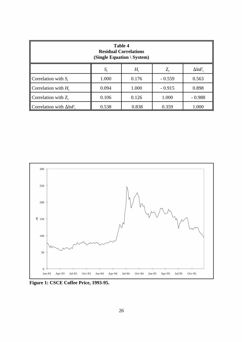
Evidence for the build-up of speculative positions in New York coffee futures may be seen

in Figure 2. Speculators established significant large positions through the summer of 1993 in10

response to the announcement of the Coffee Retention Scheme, but these were subsequently run

down and they entered 1994 with a slightly negative net position. Their positions then climbed to

a peak of around 20,000 contracts in April 1994, an investment of around $600m. After the frosts,

these positions gradually worked back down to zero at the year-end but built up again through

the spring of 1995 against the possibility of a second successive southern hemisphere winter of

frosts. These are significant sums of money in relation to the coffee market, but very small in

relation to overall equity and bond markets. What was therefore a relatively small diversification

out of those markets amounted to a very large diversification into coffee futures.

4. The Econometric Model

We specify equations for the three futures market positions (large speculators, hedgers and

noise traders). The futures price equation is inferred through the market clearing identity (6) on

the futures positions resulting in a four equation system.

Consider first the positions equations. As noted in section 2, these follow directly from

equations (4) and (19) together with random noise traders positions. However, the theoretical

model considers only a single sequence of trades, while my data consist of time series relating to

a sequence of position realizations. This has four sets of implications.

i) It is apparent from Figure 2 that positions exhibit positive serial correlation. This can be

rationalized in terms of at least some agents adjusting their futures positions less rapidly

than the weekly frequency of our data. It suggests that we regard the theoretical position

relationships as targets to which actual positions adjust over time.

ii) Hedgers tend to view the futures price in relation to their perceptions of likely prices in

the future which they will necessarily judge from past prices. I model the net hedge in

relation to the current period futures price relative to its previous value.

"0(L)St ' ")

1 It & "2 Zt % u St

$0(L)Ht ' & $3)lnFt % u Ht

(0(L) Zt ' (4)St&1 % u Zt

See footnote 9.11

An earlier draft of this paper reported a version of the model augmented by an additional12

equation for volatility. The estimates showed volatility as reducing the absolute size of both speculativeand hedge positions, but both coefficients were highly insignificant.

12

(20)

iii) The CFTC positions data attract widespread interest and comment in brokers’ circulars

to their clients and there is evidence in the data that noise traders do imitate the large

speculators. I attempt to capture this behaviour.

iv) The theoretical model supposes that coffee prices are efficient relative to each agent’s

information set, but the data exhibit mild evidence of inefficiency (see below).

The model consists of the following positions equations:

L is the lag operator and lag distributions are all second order. Here, F is the second positiont

futures price (corresponding to f in the theoretical model ) and I is a vector of informational11t

variables (" ‘I corresponds to e in the theoretical model). All coefficients (except " ) are written1 t 1

so that parameters will be positive. Each equation in (20) also contains an intercept and two

dummy variables associated with the two frost weeks in 1994, which would otherwise exert

excessive leverage .12

Model identification follows from standard exclusion restrictions. The net speculative

equation is identified through exclusion of the lagged hedge positions H and H while the hedget-1 t-2

equation is identified by exclusion of the informational variables I and the lagged speculativet

positions S and S . The noise equation is inferred from the futures market identity (6).t-1 t-2

The crucial variables are those appertaining to speculative information, denoted by I int

equations (20). As outlined in section 3, we see speculators in the CSCE coffee market over this

particular period as being informed about likely developments in the financial markets generally

rather than on coffee market fundamentals. We attempt to capture this information through

including a set of variables which are relevant to forecasting short term holding gains on equity

and bond portfolios. The three variables we include measure respectively equity returns, bond

A L yt ' 7 It & $)lnFt % ut where $ '

0$3

07 '

")

1

0)

0)

A0 '

1 0 "2

0 1 0

0 0 1

A1 '

"01 0 0

0 $01 0

&(4 0 (01

and A2 '

"02 0 0

0 $02 0

(4 0 (02

)lnFt '1$3

E2

j'14)Bjyt&j & 4)7It & 4)ut

where Bj ' A &10 Aj j'1,2 and vt ' A &1

0 ut

I am grateful to the Chicago Board of Trade for providing implied volatility data. I have taken13

volatilities from bond futures contracts with maturity closest to six months.

13

(21)

(22)

market returns and bond market volatility, as a measure of the riskiness. Precise definitions are

I = ) lnS&P the change in the Standard and Poors Composite Index over the1t 3 t

previous three weeks;

I = )YGAP - )YGAP the change in the yield gap between the redemption yields on 302t t t-3

and 10 year US government bonds over the preceding week

relative to the same change two weeks earlier; and

I = )BVOL - )BVOL the change in the implied volatility of CBT Treasury bond futures3t t-1 t-3

the preceding week relative to the same change two weeks

earlier.13

The precise measures (ie difference and lag structures) were suggested by preliminary regressions.

Note that, because only exogenous variables are differences, these transformations do not in any

way contaminate the equation disturbances.

Stacking the three position variables so that y = (S ,H ,Z )’ and writing the remainingt t t t

variables as v , the three position equations (20) may be written ast

The identity (6) implies 4'y = 0 where 4 is the vector of units allowing us to infer the solvedt

futures price equation as

B )

j 4 ' bj4 j'1, 2

)lnFt ' &1$3

4)7It % 4)vt

B1 '

"01%"2(4 0 &"2(01

0 $01 0

&(4 0 (01

and B2 '

"02&"2(4 0 &"2(02

0 $02 0

(4 0 (02

"01 ' b1 & (1&"2)(4 "02 ' b2 % (1&"2)(4

$01 ' b1 and $02 ' b2

(01 'b1

1&"2

(02 'b2

1&"2

14

(23)

(24)

(25)

(26)

(since A 7 = 7). It is natural to require that the current period futures price should not be0-1

predictable from lagged speculative and hedge positions - a market efficiency condition. This

requires

ie the column sums of the reduced form adjustment distributed lag matrices should be identical.

The futures price equation would then become

The most simple way that equation (24) might be satisfied is if each of the two matrices B werej

proportional to the identity matrix. However, model fit is improved by permitting noise traders

to imitate speculative positions with a one week lag; and conditioning speculative positions on the

noise positions introduces further off-diagonal elements. One may evaluate

Noting that the second columns of both B and B each contain a single element, the column sum1 2

restrictions (23) may be written as

However, there is also some evidence that lagged positions do have some effect on the futures

price, implying a degree of semi-strong inefficiency. This may be accounted for by inclusion of the

)lnFt ' &1$3

4)7 It % N)Zt&1 % 4)vt

(01 'b1

1&"2

% N and (02 'b2

1&"2

& N

"01 % "02 ' $01 % $02

Because the lagged positions sum to zero, I cannot identify which of the lagged positions affect14

the futures price. The specification in (27) is one of many possibilities.

The CFTC reports only the positions and not the numbers of small speculators. Table 1 omits15

the generally small number of non-commercial traders reported as spreading.

15

(27)

(28)

(29)

lagged change in the noise position in equation (24) which becomes14

so that (26) is modified such that

Notice that, with this modification, equations (26) only impose the single restriction

since the noise equation is dropped in estimation and hence ( must be inferred from the estimated4

speculative and hedge equations.

5. Results

The model was estimated on data from the CSCE for the ‘C’ contract covering the 156

week period from January 1993 to December 1995. Table 1 summarizes the position data. Note

C Large speculators were generally but not invariably net long, while hedgers were generally

but not invariably net short. Small speculators were net long throughout the period.

C The net hedge positions showed the greatest variability and the net small speculative

position the least variability. The net hedge and large speculative positions were strongly

negatively correlated, while the small speculative position was positively correlated with

the large speculative position. These correlations confirm the visual impression given by

Figure 2.

C Turning to the number of reporting traders, large speculators were predominantly long15

while hedgers were much more evenly balanced. The greatest variability was in the number

16

of long large speculators.

These numbers are consistent with a characterization of the CSCE markets as operating with a

relatively small and consistent group of traders but which experienced an influx of non-traditional

large speculators taking predominantly long positions.

Model estimation results are reported in Tables 2-4. Tables 2 reports single equation (OLS

or IV) estimation of the position equations together with the implied futures price equation, while

Table 3 reports FIML system estimates of the same equations. The estimates reported in Table

2 impose only the intra-equation restrictions while those reported in Table 3 impose both intra-

and inter-equation restrictions. Table 4 reports the correlation matrices of the single equation

residuals and the structural residuals from the system estimates.

Considering first the estimated equations for the net large speculative positions (Tables 2

and 3, column 1), the coefficients " on the three informational variables I (j=1,2,3) are well-1j jt

determined and differ little between the two estimation procedures. These estimates provide

strong support for the contention that speculators were motivated to invest in coffee by

consideration of financial rather than coffee fundamentals in this period. The coefficient " on the2

noise positions Z is incorrectly signed in the single equation estimates, but correctly signed,t

although insignificant, in the system estimates.

Turning to the estimated net hedge equations (Tables 2 and 3, column 2), note that it is

necessary to reverse the signs on the estimated coefficients when interpreting effects on the size

of the hedge position in view of the fact hedgers are almost invariably net short. The effects of

changes in the futures price on the hedge position are clear and in line with the theoretical model

developed in section 2. A rise in the futures price lnF results in an increase in the net shortt

position.

For completeness, the coefficients in the noise (small speculators) equation implied by the

FIML estimates are also tabulated together with OLS estimates for purposes of comparison

(Tables 2 and 3, column 3). The coefficient estimates are fairly similar, but there is in this case a

substantial deterioration in fit in moving from the single equation to the system estimates. As

might be expected from market efficiency considerations, the single equation estimates of the

futures price equation (Table 2, column 4) are very poorly determined. The FIML estimates of the

same equation (Table 3, column 4) derive almost entirely from the imposition of cross-equation

restrictions.

One might consider imposing the restrictions in sequence testing each set in turn. The problem16

with this approach is that the acceptability of a given set of restrictions is not independent of the sequenceorder and no “natural” ordering suggests itself in the current context. In practice it was found that anygiven subset of restrictions was less acceptable the later in the sequence it was imposed. The mostproblematic restrictions were the cross equation restrictions on the futures price equation implied byequation (30) and the restriction that the bottom left hand elements of the polynomial distributed lagmatrices A and A in (30) be equal and opposite. The equation diagnostics suggest significant departures1 2

from normality on all equations, and this indicates caution with regard to reported t values and P statistics.2

17

Overall, the system estimates impose a total of 12 over-identifying restrictions. A

likelihood ratio test indicates that the set of restrictions is acceptable at the 5% level. The16

residual correlations reported in Table 4 (single equation estimates on the sub-diagonal and system

estimates on the super-diagonal) should be compared with the correlations of the raw variables

in Table 1. The residuals from the speculative and hedge positions are near independent, while

the raw variables are strongly negatively correlated. Note also the high correlation of the residuals

from the futures price equation with the position residuals. High residual cross-equation

correlations are consistent with the theoretical model in which the futures price disturbances are

a linear combination of the position disturbances - see equations (20) and (21). Overall, therefore,

we regard the systems estimates, reported in Table 3 as providing a satisfactory representation of

the econometric model elaborated in section 4, and as representing the theoretical model

developed in section 2.

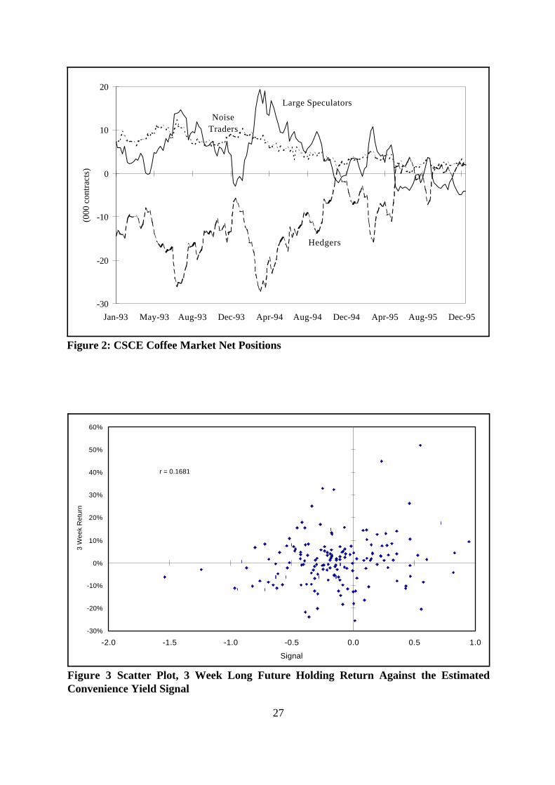
This view may be corroborated by reconstruction of the convenience yield signal e ,t

estimated as " ’I . The correlation of this estimated signal does indeed turn out to be positively1 t

correlated with the return to holding a long futures position over the following weeks. The

correlation is maximized for a three week holding period with a value of r = 0.168 - see Figure

3 for the scatter plot. This correlation is significantly different from zero at conventional

significance levels. And although this particular correlation is reduced if the frost period in mid-

1994 is excluded from the sample, it remains positive, and is actually higher than the value quoted

for slightly longer holding periods. At least with regard to coffee, therefore, speculators were

correct in judging that possibly poor returns and increased riskiness of equity and bond

investments made diversification into physical commodities attractive.

6. Conclusions

A general difficulty with models which rely on asymmetry of information is that it is

Phillips and Weiner (1994) find that speculators in the Brent oil forward market have no17

informational advantage. However, all traders in this market are either large national or international oilrefining companies or major international banks and it seems entirely plausible, in that context, that allwould have access to and be familiar with the same information.

18

difficult to work out who knew what and when they know this. This in turn makes it difficult to

test these models econometrically. We have sought to overcome this problem by looking at a short

historical period in which an influx of non-traditional traders entered the physical commodity

markets. 1994 saw a large movement of speculative money into commodities, motivated by

portfolio diversification considerations in the face of likely poor equity and bond returns in the

face of the probability of rising interest rates. Although this information was available to traditional

traders in these markets, and in particular to hedgers, it was not information which they had come

to regard as relevant. This implies a degree of informational segmentation in the market.

Within this context we have developed a model in which informed speculators receive

signals relating to price developments, and establish futures positions on the basis of these signals.

A bullish signal results in speculators establishing a long position thereby bidding up the futures

price. Hedgers, observing the price rise but not the information which generated it, are unsure as

to whether it is due to informed speculation or to random noise trading. The consequence is that,

even though the rise in the futures price raises their expectation of the future cash price, this is not

by so much as the rise in the futures price, and they shorten their futures positions.

This was the observed sequence of events in the New York coffee futures market during

1994. We have reported estimates of an econometric model of the coffee futures market which

provide support for the segmentation hypothesis. This model is relatively successful in accounting

for the comovement of the speculative and hedge positions. Furthermore, we have been able to

reconstruct an estimate of the signal received by speculators and demonstrate that this is positively

correlated with futures holding returns. This does not demonstrate the profitability of ant actual

speculative behaviour, but does establish that any speculators who took notice of this information

would have been able to partially anticipate subsequent price movements.

Our estimates relate to a particular market in a particular time period. We do not claim any

generality for the informational partition which we have been able to exploit in this particular

instance. Rather, this should be taken as a cast study, in which we have been able to use the17

modern theory of price discovery in financial markets to explain a set of events which market

contemporary market participants found hard to understand. This theory does have general

19

application, and the general structure of the argument, although not the particular model, will be

relevant in a number of contexts. Examples might include learning from central bank support

operations in foreign exchange markets and leaning about possible manipulative trades in

commodity futures markets.

20

Appendix: Variable Definitions and Sources

BVOL Implied volatilities of CBT options on Treasury bond futures with approximatelysix months to maturity (CBT).

F Second position price, CSCE, ¢/lb, Tuesdays (FDI).See footnote 9 on rolling. H Net long reportable positions of commercial traders on the CSCE, Tuesdays,

contracts of 36,500 lbs (CFTC).P First position price, CSCE, ¢/lb, Tuesdays (FDI). See footnote 9 on rolling. S Net long reportable positions of non-commercial traders on the CSCE, Tuesdays,

contracts of 36,500 lbs (CFTC).S&P Standard and Poors Composite Index (DS).YGAP Redemption yield on 30 year US Treasury bond less redemption yield on 10 year

US Treasury bond, Tuesdays, (constructed; bond yields: DS).Z Net long non-reportable positions of non-commercial traders on the CSCE,

Tuesdays, contracts of 36,500 lbs (CFTC).

CBT Chicago Board of TradeCFTC Commodity Futures Trading Commission, Commitments of Traders in Futures,

Washington, DCDS Datastream Ltd, London.FDI Futures Data Institute, Washington, DC

The data used in this study are available from the author on request.

21

References

Bessembinder, H. (1992), “Systematic risk, hedging pressure, and risk premiums in futuresmarkets”, Review of Financial Studies, 5, 637-67.

Chang, E.C. (1985), “Returns to speculators and the theory of normal backwardation”, Journalof Finance, 40, 193-208.

De Long, J.B., Shleifer, A., Summers, L.H., and Waldmann, R.J. (1990), “Positive feedbackinvestment strategies and destabilizing rational expectations”, Journal of Finance, 45. 379-95.

De Long, J.B., Shleifer, A., Summers, L.H., and Waldmann, R.J. (1991), “The survival of noisetraders in financial markets”, Journal of Business, 64, 1-19.

Edwards, F.R., and Ma, C.W. (1992), Futures and Options, New York, McGraw-Hill.

Gilbert, C.L., and Brunetti, C. (1997), Speculation, Hedging and Volatility in the Coffee Market,1993-96, Department of Economics, Queen Mary and Westfield College, Occasional Paper.

Grossman, S.J. (1977), “The efficiency of futures markets, noisy rational expectations andinformational externalities”, Review of Economic Studies, 44, 431-49.

Grossman, S.J., and Stiglitz, J.E. (1980), “On the impossibility of informationally efficientmarkets”, American Economic Review, 61, 393-408.

Hartzmark, M.L. (1987), “Returns to individual traders of futures: aggregate results”, Journal ofPolitical Economy, 95, 1292-1306.

Houthakker, H.S. (1957), “Can speculators forecast prices?”, Review of Economics and Statistics,39, 143-51.

International Coffee Organization (1999), Coffee Statistics, December 1998, 13, London,International Coffee Organization.

Kyle, A.S. (1985), “Continuous auctions and insider trading”, Econometrica, 53, 1315-35.

Phillips, G.M., and Weiner, R.J. (1994), “Information and normal backwardation as determinantsof trading performance: evidence from the North Sea oil forward market”, Economic Journal,104, 76-95.

Rochet, J.-C., and Vila, J.-L. (1994), “Insider trading without normality”, Review of EconomicStudies, 61, 131-52.

Rockwell, C.S. (1977), “Normal backwardation and the returns to commodity futures traders”,in Peck, A.E. ed., Selected Writings on Futures Markets, 2, Chicago, Chicago Board of Trade.

Satyanarayan, S., and Varangis, P. (1994), “An efficient frontier for international portfolios with

22

commodity assets”, Policy Research Working Paper 1266, World Bank International EconomicsDepartment, Washington D.C., World Bank.

Shalen, C.T. (1993), “Volume, volatility and dispersion of beliefs”, Review of Financial Studies,6, 405-34.

Wadhwani, S., and Shah, M. (1993), “Commodities and portfolio performance”, Goldman SachsPortfolio Strategy, 30 September 1993.

Yoo, J., and Maddala, G.S. (1991), “Risk premia and price volatility in futures markets”, Journalof Futures Markets, 11, 165-77.

23

Table 1Descriptive Statistics and Correlations

Positions (contracts) S H Z

Mean 4,577 - 10,132 5,555

Standard deviation 5,593 7,664 2,932

Minimum - 4,961 - 27,173 322

Maximum 19,333 3,594 12,229

Position correlations S H Z

Correlation with S 1.000

Correlation with H - 0.952 1.000

Correlation with Z 0.592 - 0.810 1.000

Numbers of Traders long, short long, short

Mean 43 , 22 56 , 41

Standard deviation 18 , 9 8 , 5

Minimum 17 , 5 41 , 27

Maximum 80 , 43 78 , 54

24

Table 2Single Equation Estimates

S H Z )nFt

(IV) (IV) (OLS) (OLS)t t t

S 1.0282 0.0716t-1

(12.9) (2.23)

S -0.1448 -0.0716t-2

(1.90) (*)

H 1.2116t-1

(10.1)

H -0.3379t-2

(2.31)

Z 0.1330t

(2.01)

Z 0.7143 -0.0033t-1

(9.36) (0.58)

Z 0.2528 0.0033t-2

(3.31) (*)

)lnF -69.052t

(1.42)

I - 18.434 -0.41951,t

(2.04) (1.50)

I - 4.531 0.03092,t

(1.79) (0.27)

I 0.7689 0.00073,t

(2.32) (0.07)

R (OLS) 0.928 0.068 2

standard error 1.877 3.254 0.801 0.060 serial correlation P = 3.94 P = 1.33 P = 5.92 P = 6.54heteroscedasticity P = 9.14 P = 123 P = 6.76 P = 10.8normality P = 15.5 P = 31.9 P = 1.81 P = 18.4

24

214

22

24

28

22

24

28

22

24

210

22

Restrictions P = 3.30 P = 4.00 21

24

Notes: Equations also contain constant and two frost dummies; see appendix forvariable definitions; asymptotic t statistics in parentheses; * indicates a restrictedcoefficient; italicized P values are significant at the 95% level. 2

25

Table 3FIML System Estimates

S H Z )nFt t t t

S 1.1067 0.0836t-1

(17.7) (*)

S - 0.1855 - 0.0836t-2

(2.94) (*)

H 1.1884t-1

(17.6)

H - 0.2672t-2

(*)

Z - 0.0227t

(0.95)

Z 0.7841 - 0.00647t-1

(*) (1.98)

Z - 0.2734 0.00648t-2

(*) (*)

)lnF - 81.302t

(2.11)

I - 20.535 - 0.25261,t

(2.33) (*)

I - 4.912 - 0.06042,t

(1.97) (*)

I 0.8683 0.010683,t

(2.64) (*)

standard error 1.911 3.919 4.562 0.0601serial correlation P = 1.40 P = 6.29 P = 4.90 P = 5.36heteroscedasticity P = 12.4 P = 9.92 n.a. P = 16.8normality P = 13.2 P = 13.7 P = 22.9 P = 23.1

24

214

22

24

214

22

24

22

24

214

22

Restrictions P = 19.2212

Notes: See Table 2.

0

50

100

150

200

250

300

Jan-93 Apr-93 Jul-93 Oct-93 Jan-94 Apr-94 Jul-94 Oct-94 Jan-95 Apr-95 Jul-95 Oct-95

c/lb

26

Figure 1: CSCE Coffee Price, 1993-95.

Table 4Residual Correlations

(Single Equation \ System)

S H Z )lnFt t t t

Correlation with S 1.000 0.176 - 0.559 0.563t

Correlation with H 0.094 1.000 - 0.915 0.898t

Correlation with Z 0.106 0.126 1.000 - 0.988t

Correlation with )lnF 0.538 0.838 0.359 1.000t

-30

-20

-10

0

10

20

Jan-93 May-93 Aug-93 Dec-93 Apr-94 Aug-94 Dec-94 Apr-95 Aug-95 Dec-95

(000

con

trac

ts)

Large Speculators

Hedgers

NoiseTraders

-30%

-20%

-10%

0%

10%

20%

30%

40%

50%

60%

-2.0 -1.5 -1.0 -0.5 0.0 0.5 1.0

Signal

3 W

eek

Ret

urn

r = 0.1681

27

Figure 2: CSCE Coffee Market Net Positions

Figure 3 Scatter Plot, 3 Week Long Future Holding Return Against the EstimatedConvenience Yield Signal