Embed Size (px)
Citation preview

INFORMATIVE TRANSITIONS 1
How People Learn about Causal Influence when there are Many Possible Causes: A Model
Based on Informative Transitions
Cory Derringer and Benjamin Margolin Rottman
University of Pittsburgh
This research was supported by NSF Grant 1430439. Parts of this research were presented at the
Cognitive Science Conference (Derringer & Rottman, 2016).
INFORMATIVE TRANSITIONS 2
Abstract
Four experiments tested how people learn cause-effect relations when there are many possible
causes of an effect. When there are many cues, even if all the cues together strongly predict the
effect, the bivariate relation between each individual cue and the effect can be weak, which can
make it difficult to detect the influence of each cue. We hypothesized that when detecting the
influence of a cue, in addition to learning from the states of the cues and effect (e.g., a cue is
present and the effect is present), which is hypothesized by multiple existing theories of learning,
participants would also learn from transitions – how the cues and effect change over time (e.g., a
cue turns on and the effect turns on). We found that participants were better able to identify
positive and negative cues in an environment in which only one cue changed from one trial to the
next, compared to multiple cues changing (Experiments 1A, 1B). Within a single learning
sequence, participants were also more likely to update their beliefs about causal strength when
one cue changed at a time (‘one-change transitions’) than when multiple cues changed
simultaneously (Experiment 2). Furthermore, learning was impaired when the trials were
grouped by the state of the effect (Experiment 3) or when the trials were grouped by the state of
a cue (Experiment 4), both of which reduce the number of one-change transitions. We developed
a modification of the Rescorla-Wagner algorithm to model this ‘Informative Transitions’
learning processes.
INFORMATIVE TRANSITIONS 3
How People Learn about Causal Influence when there are Many Possible Causes: A Model
Based on Informative Transitions
1. Introduction
Learning the strengths of causal relations is essential for successfully predicting and
manipulating the environment. For example, a student might consider the merits of staying
awake one extra hour to study for a test. Knowing the extent to which one more hour of studying
would improve or harm her score would help her decide whether more studying is worthwhile.
However, causal relations do not exist in isolation; often there are multiple causes that influence
an effect in different ways. A student might attend class and do homework assignments (positive
influences on test performance), but might study by cramming and doze off during class
(negative influences). Further, the causes could be correlated; one more hour of studying may
mean one less hour of sleep. In the same way that statisticians use regression to formally
estimate the effect of one independent variable above and beyond another, individuals should
attempt to control for alternative causes to estimate the unique strength of a target cause in
informal causal learning situations.
Causal learning generally, and controlling for variables in particular, has historically been
of interest to three areas of psychology. First, social psychologists have long studied the causal
attribution process – how individuals attribute the occurrence of an event to one of multiple
potential causes. Kelley (1973) famously suggested that lay people use a process similar to
running a mental analysis of variance (ANOVA) to determine which causes are responsible for
the effect. Second, cognitive psychologists have demonstrated in multiple ways that people do in
fact control for alternative causes when estimating the influence of a target cause (e.g., Spellman,
1996; Spellman, Price, & Logan, 2001; Waldmann & Holyoak, 1992; Waldmann, 2000;
INFORMATIVE TRANSITIONS 4
Waldmann & Hagmayer, 2001). Third, controlling for variables has also been a focus of research
in education psychology and developmental psychology as it is one of the important processes
that goes into successful scientific reasoning (Cook, Goodman, & Schulz, 2011; Chen & Klahr,
1999; Kuhn & Dean, 2005; Schulz & Bonawitz, 2007).
However, one limitation of the foundational cognitive studies mentioned above is that
they have primarily focused on whether and when people control for alternative causes, not the
process through which learners control for alternative causes. Thus, one of the primary goals of
the current research is to develop a better understanding of how learners control for alternative
causes.
Another limitation is that most of the prior research on how people infer causal influence
has focused on learning about a single cause at a time (e.g., Cheng, 1997; Griffiths &
Tenenbaum, 2005; Hattori & Oaksford, 2007), or learning about two or three causes
simultaneously (see citations above). However, many real-world outcomes (e.g., number of
hours of sleep per night) have large numbers of factors that could be causes (e.g., diet, exercise,
caffeine, computer use before bed, environmental noise, stress, eating a midnight snack, eating
dessert, weather, taking a melatonin supplement, allergies, water consumption, alcohol
consumption, etc.). A few studies have investigated situations in which there are larger numbers
of causes (e.g., Vandorpe & De Houwer, 2006); however, studies like this often use a paradigm
in which only one or two causes are present on a given trial, which can simplify learning if the
learner focuses on the few causes that are present at a time. In real world learning situations often
multiple causes occur simultaneously (e.g., caffeine, using a computer before bed, environmental
noise, stress, a midnight snack, etc.). Another related issue is that for any particular outcome,
there are unlimited numbers of factors that are not causes of the outcome (cf. the Frame Problem
INFORMATIVE TRANSITIONS 5
in Philosophy, Shanahan, 2016). Learners must distinguish between the factors that have a causal
influence and those that do not. For these reasons, the second major focus of the current research
is how people learn about causes in situations in which there are many, in our experiments eight,
potential causes of a given effect, and the learner’s goal is to figure out 1) which factors are
causes and which are not, and 2) if they are causes, whether they have a positive or negative
influence.
In the current article, we are particularly interested in comparing how people learn about
the causal influence of many potential causes in an environment in which the potential causes are
fairly stable or ‘autocorrelated’ over time vs. environments in which the causes change randomly
from trial to trial (low autocorrelation). For example, when considering the factors that might
influence the number of hours of sleep per night, many of the factors are likely to come and go in
waves (e.g., stress, environmental noise, allergies, etc.). We hypothesize that people may learn
about potential causes more easily when they are autocorrelated, and put forth a theory to explain
why.
The outline for this article is as follows. First, we introduce an example set of learning
data and some intuitive hypotheses about how people will learn from these data. Second, we
review two theories of learning about multiple causes: multiple regression, and the Rescorla-
Wagner model (Rescorla & Wagner, 1972). (A third theory, focal sets, is discussed in the general
discussion (Cheng & Novick, 1990; Cheng & Holyoak, 1995).) Then we propose another theory
of causal learning, which we call ‘Informative Transitions,’ and introduce two versions of a
model based on learning causal strengths through transitions. Finally, we report four experiments
to test when learners update their beliefs about causal strength in a trial-by-trial learning
paradigm.
INFORMATIVE TRANSITIONS 6
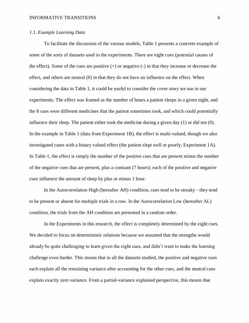
1.1. Example Learning Data
To facilitate the discussion of the various models, Table 1 presents a concrete example of
some of the sorts of datasets used in the experiments. There are eight cues (potential causes of
the effect). Some of the cues are positive (+) or negative (-) in that they increase or decrease the
effect, and others are neutral (0) in that they do not have an influence on the effect. When
considering the data in Table 1, it could be useful to consider the cover story we use in our
experiments. The effect was framed as the number of hours a patient sleeps in a given night, and
the 8 cues were different medicines that the patient sometimes took, and which could potentially
influence their sleep. The patient either took the medicine during a given day (1) or did not (0).
In the example in Table 1 (data from Experiment 1B), the effect is multi-valued, though we also
investigated cases with a binary valued effect (the patient slept well or poorly; Experiment 1A).
In Table 1, the effect is simply the number of the positive cues that are present minus the number
of the negative cues that are present, plus a constant (7 hours); each of the positive and negative
cues influence the amount of sleep by plus or minus 1 hour.
In the Autocorrelation High (hereafter AH) condition, cues tend to be streaky - they tend
to be present or absent for multiple trials in a row. In the Autocorrelation Low (hereafter AL)
condition, the trials from the AH condition are presented in a random order.
In the Experiments in this research, the effect is completely determined by the eight cues.
We decided to focus on deterministic relations because we assumed that the strengths would
already be quite challenging to learn given the eight cues, and didn’t want to make the learning
challenge even harder. This means that in all the datasets studied, the positive and negative cues
each explain all the remaining variance after accounting for the other cues, and the neutral cues
explain exactly zero variance. From a partial-variance explained perspective, this means that

INFORMATIVE TRANSITIONS 7
learners should judge the positive and negative cues as extremely strong, and weak judgments
are a sign of difficulty learning about or difficulty controlling for the other cues (see the method
sections for more details about the stimuli).
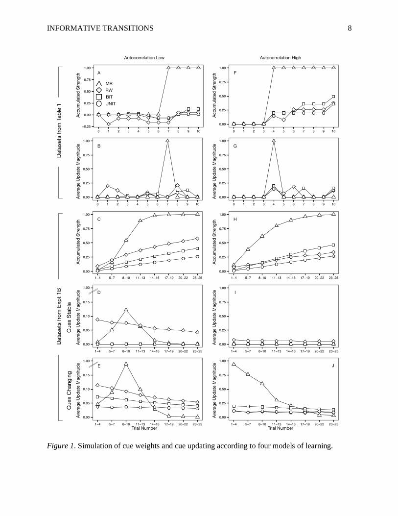
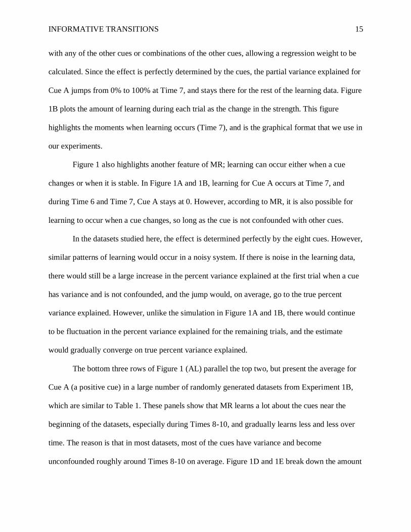
The top two rows of Figure 1 present simulations of four models of causal strength
learning applied to Cue A in Table 1. The bottom three rows present simulations of the four
models applied to all the learning datasets used in Experiment 1B, to show the predictions of the
models when aggregated across all the data sets. Table 1 and Figure 1 will be extensively
discussed in the following sections.
Table 1
Example learning data.
Autocorrelation Low (AL) Autocorrelation High (AH)
Time 1 2 3 4 5 6 7 8 9 10 1 2 3 4 5 6 7 8 9 10
Trial # 4 10 2 8 5 1 9 6 3 7 1 2 3 4 5 6 7 8 9 10
Cue A+ 1 1 0 0 1 0 0 1 0 0 0 0 0 1 1 1 0 0 0 1
Cue B+ 0 0 0 0 0 1 0 0 0 0 1 0 0 0 0 0 0 0 0 0
Cue C+ 0 1 0 1 0 0 1 1 0 1 0 0 0 0 0 1 1 1 1 1
Cue D0 1 0 1 0 0 1 0 0 1 0 1 1 1 1 0 0 0 0 0 0
Cue E0 0 0 0 0 0 0 0 0 0 0 0 0 0 0 0 0 0 0 0 0
Cue F- 1 0 1 0 1 1 0 1 1 1 1 1 1 1 1 1 1 0 0 0
Cue G- 0 1 0 0 0 0 1 0 0 0 0 0 0 0 0 0 0 0 1 1
Cue H- 1 1 0 1 1 0 1 1 1 1 0 0 1 1 1 1 1 1 1 1
Effect 6 7 6 7 6 7 6 7 5 6 7 6 5 6 6 7 6 7 6 7
Note. +, -, and 0 denote positive, negative, and neutral cues.
INFORMATIVE TRANSITIONS 8
Figure 1. Simulation of cue weights and cue updating according to four models of learning.
INFORMATIVE TRANSITIONS 9
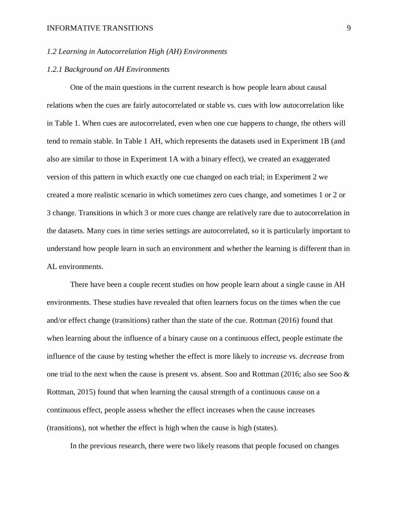
1.2 Learning in Autocorrelation High (AH) Environments
1.2.1 Background on AH Environments
One of the main questions in the current research is how people learn about causal
relations when the cues are fairly autocorrelated or stable vs. cues with low autocorrelation like
in Table 1. When cues are autocorrelated, even when one cue happens to change, the others will
tend to remain stable. In Table 1 AH, which represents the datasets used in Experiment 1B (and
also are similar to those in Experiment 1A with a binary effect), we created an exaggerated
version of this pattern in which exactly one cue changed on each trial; in Experiment 2 we
created a more realistic scenario in which sometimes zero cues change, and sometimes 1 or 2 or
3 change. Transitions in which 3 or more cues change are relatively rare due to autocorrelation in
the datasets. Many cues in time series settings are autocorrelated, so it is particularly important to
understand how people learn in such an environment and whether the learning is different than in
AL environments.
There have been a couple recent studies on how people learn about a single cause in AH
environments. These studies have revealed that often learners focus on the times when the cue
and/or effect change (transitions) rather than the state of the cue. Rottman (2016) found that
when learning about the influence of a binary cause on a continuous effect, people estimate the
influence of the cause by testing whether the effect is more likely to increase vs. decrease from
one trial to the next when the cause is present vs. absent. Soo and Rottman (2016; also see Soo &
Rottman, 2015) found that when learning the causal strength of a continuous cause on a
continuous effect, people assess whether the effect increases when the cause increases
(transitions), not whether the effect is high when the cause is high (states).
In the previous research, there were two likely reasons that people focused on changes
INFORMATIVE TRANSITIONS 10
when learning cause-effect relations in AH environments. First, changing cues might be more
salient than stable cues. The second reason is from a computational perspective. Using the
changes in variables over time rather than their states is a cognitively simple way to account for
non-stationarity or autocorrelation when performing inferential statistics on time-series data
(Rottman, 2016; Shumway & Stoffer, 2011). However, all the previous research on transitions
involved just one potential cause; in the current research we investigate how people learn about
many potential causes.
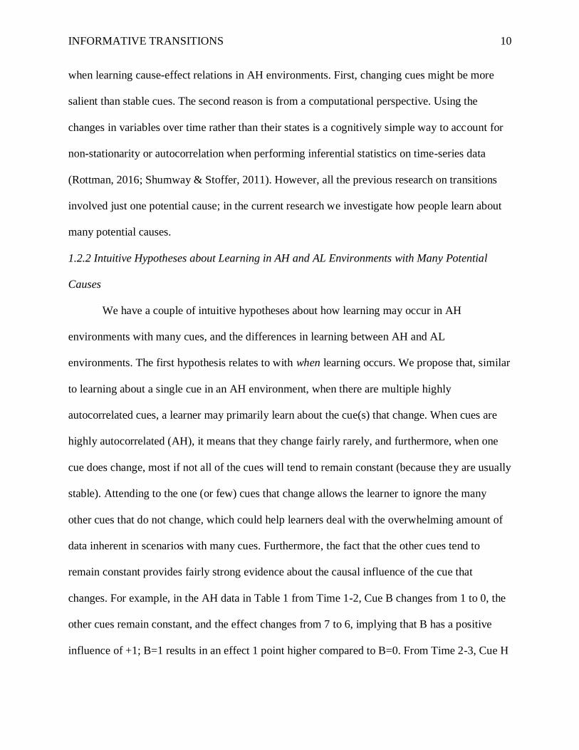
1.2.2 Intuitive Hypotheses about Learning in AH and AL Environments with Many Potential
Causes
We have a couple of intuitive hypotheses about how learning may occur in AH
environments with many cues, and the differences in learning between AH and AL
environments. The first hypothesis relates to with when learning occurs. We propose that, similar
to learning about a single cue in an AH environment, when there are multiple highly
autocorrelated cues, a learner may primarily learn about the cue(s) that change. When cues are
highly autocorrelated (AH), it means that they change fairly rarely, and furthermore, when one
cue does change, most if not all of the cues will tend to remain constant (because they are usually
stable). Attending to the one (or few) cues that change allows the learner to ignore the many
other cues that do not change, which could help learners deal with the overwhelming amount of
data inherent in scenarios with many cues. Furthermore, the fact that the other cues tend to
remain constant provides fairly strong evidence about the causal influence of the cue that
changes. For example, in the AH data in Table 1 from Time 1-2, Cue B changes from 1 to 0, the
other cues remain constant, and the effect changes from 7 to 6, implying that B has a positive
influence of +1; B=1 results in an effect 1 point higher compared to B=0. From Time 2-3, Cue H
INFORMATIVE TRANSITIONS 11
changes from 0 to 1, and the effect changes from 6 to 5, implying that H has a negative influence
of -1. From Time 4-5, Cue D changes from 1 to 0, and the effect does not change, implying that
D has no influence on the effect. Statistically, these transitions in which only one cue changes are
especially informative for learning about the influence of the variable that changed, because all
the other cues are held constant. For this reason, we further predict not just that people will
primarily learn about cues that change, but that they will learn more when a single cue changes
than when multiple cues change simultaneously.
The second hypothesis relates to the consequences of focusing on changes. If learners
focus on changes, then they should be able to fairly accurately learn the causal relations in an AH
environment. For the AH dataset in Table 1, they should be able to learn that the positive cues
have a strong positive influence, that the negative cues have a strong negative influence, and that
the neutral cues have no influence. Likewise, when asked to predict the effect on a given trial,
their predictions should be quite accurate.
A third hypothesis has to do with the difference between the AH and AL environments.
Given the prevalence of AH environments in everyday learning, we hypothesize that people
might also focus on changes even in AL environments. Furthermore, people tend to think that
variables are positively autocorrelated even when they have zero autocorrelation, so they might
attend to changes merely because they fail to realize that the data are not autocorrelated (e.g.
Lopes & Oden, 1987; Wagenaar, 1970; but also see debates about the hot hand fallacy vs. the
gambler’s fallacy, reviewed by Oskarsson, Van Boven, McClelland & Hastie, 2009).
If people focus on changes in the AL environment, then learning would be worse in the
AL environment compared to the AH environment. In the AL environment, often multiple cues
change from one observation to the next, which could confuse subjects and slow learning. For
INFORMATIVE TRANSITIONS 12
example, if two cues change, and the effect increases by 1, it could be that one of the cues is
responsible and the other cue is neutral, or that both of them have a small influence. If three or
more cues change simultaneously the possibilities grow much larger. For this reason, we
hypothesize that subjects will learn better in AH than AL environments.
Using change-score analyses is one normative approach to deal with time series data
(AH). Is it wrong to learn from changes in an AL environment? Technically, in AL environments
people should not use changes. However, the consequences of doing so are not all that bad from
a normative perspective. In the data in the current study (e.g., Table 1), if one performs a
multiple regression on the first-order change scores of each of the eight cues and the effect, the
final causal strength estimates are exactly the same as if performed on the raw data, although the
change score regression learns slightly more slowly during the first 10 trials. Other simulations
we have performed using regression on first-order change scores have demonstrated that they
perform almost as well as just using the raw data in AL environments, and perform much better
in AH environments (Rottman, 2016; Soo & Rottman, under review). In AL environments, the
change-score analyses asymptote to the right values with large sample sizes, and have slightly
move variance in the estimates with small sample sizes, which can be viewed as a slight slowing
of learning.
In the following two sections we compare two models, Multiple Regression, and
Rescorla-Wagner, on how they perform in AH vs. AL environments to see if they capture any of
these hypotheses. Subsequently we introduce two versions of a new model designed to capture
them.
INFORMATIVE TRANSITIONS 13
1.3. Multiple Regression
1.3.1 Theory
We view multiple regression (MR) as the optimal model for calculating the influence of
each potential cause (cue) on the effect, while controlling for the other cues.1 Our experiments
involve trial-by-trial causal learning, so we implement MR by running it after each trial to
determine how the regression outputs change with each new experience. Traditionally, MR has
been viewed as a computational-level theory within psychology (Dawes & Corrigan, 1974;
Hogarth & Karelaia, 2007; Kahneman & Tversky, 1973), and because it would require
remembering all the previously experienced data, we do not view it as a psychologically
plausible way to learn about a large number of cues. Still, MR is valuable as the optimal model
against which learning can be compared, and because it makes two interesting predictions about
when learning occurs.
First, according to MR, nothing can be learned about cues with zero variance – the first
time that MR can estimate a regression weight for a cue is after the cue has been observed as
both present and absent for at least one trial each. This idea, that learning occurs when the target
cue changes (at least the first time that the cue changes), is one of the main empirical questions
of the four experiments.
1 We view Bayesian multiple regression (e.g., Kruschke, 2011) as essentially equivalent to
standard MR for the purposes of this manuscript. We did not consider a Bayesian model to learn
Causal Power, which assumes noisy-OR or noisy-AND-NOT functional forms (Cheng, 1997).
Historically, learning Causal Power has relied upon using focal sets (Cheng, 1997), which
becomes problematic with many cues. (See Section 7.2.) We do not know of an algorithm that
can learn Causal Power for a large number of cues, each of which could be generative or
inhibitory, as can be done with regression. Lastly, we note that even though noisy-OR and noisy-
AND-NOT functional forms have been dominant within the psychology research on causal
learning and reasoning, in machine learning, historically the functional forms used in regression
– linear Gaussian models and logistic models – have been the primary functional forms used for
causal structure modeling (e.g., Heckerman, 1998).
INFORMATIVE TRANSITIONS 14
The second psychologically important aspect of MR is that it does not estimate regression
weights for cues that are perfectly confounded with other cues or with linear combinations of
other cues. For example, if on the first two learning trials two cues are both off, and then both on,
even though the cues have variance, MR still cannot estimate a weight for these cues.
Technically, software packages often estimate a weight for one of the confounded variables and
drop the others. However, this decision of which cue to report is arbitrary - it depends on the
order of the variables in the model. In our simulations, we treat both variables as if no regression
weight can be calculated, to avoid arbitrarily privileging one. This question of what individuals
learn about two or more cues that change simultaneously is another of the main empirical
questions studied in the four experiments.
One important point about our simulations for MR is that we use partial variance
explained by a given cue as the metric of causal strength. We use partial variance explained
instead of the regression weights because unstandardized regression weights are not measures of
effect size.
1.3.2 MR Applied to the Autocorrelation Low (AL) Data in Table 1 as an Example
These two principles of MR (no learning with no variance or with perfect confounds) can
be seen in AL data in Table 1 as well as Figure 1A and 1B. Nothing can be learned about Cue A
during Times 1 and 2 because A=1 for both trials (variance is zero). At Time 3, A=0 so A has
variance; however, at Time 3, Cue A is still perfectly correlated with Cue H, which means that
separate estimates cannot be reached for these two cues. For this reason, we still code A as
explaining zero percent of the variance (partial variance explained) in Figure 1A. At Time 4, A is
no longer perfectly confounded with any of the other cues, but it is still confounded with a linear
combination of the other cues: A = G + H - C. Time 7 is the first time that A is not confounded
INFORMATIVE TRANSITIONS 15
with any of the other cues or combinations of the other cues, allowing a regression weight to be
calculated. Since the effect is perfectly determined by the cues, the partial variance explained for
Cue A jumps from 0% to 100% at Time 7, and stays there for the rest of the learning data. Figure
1B plots the amount of learning during each trial as the change in the strength. This figure
highlights the moments when learning occurs (Time 7), and is the graphical format that we use in
our experiments.
Figure 1 also highlights another feature of MR; learning can occur either when a cue
changes or when it is stable. In Figure 1A and 1B, learning for Cue A occurs at Time 7, and
during Time 6 and Time 7, Cue A stays at 0. However, according to MR, it is also possible for
learning to occur when a cue changes, so long as the cue is not confounded with other cues.
In the datasets studied here, the effect is determined perfectly by the eight cues. However,
similar patterns of learning would occur in a noisy system. If there is noise in the learning data,
there would still be a large increase in the percent variance explained at the first trial when a cue
has variance and is not confounded, and the jump would, on average, go to the true percent
variance explained. However, unlike the simulation in Figure 1A and 1B, there would continue
to be fluctuation in the percent variance explained for the remaining trials, and the estimate
would gradually converge on true percent variance explained.
The bottom three rows of Figure 1 (AL) parallel the top two, but present the average for
Cue A (a positive cue) in a large number of randomly generated datasets from Experiment 1B,
which are similar to Table 1. These panels show that MR learns a lot about the cues near the
beginning of the datasets, especially during Times 8-10, and gradually learns less and less over
time. The reason is that in most datasets, most of the cues have variance and become
unconfounded roughly around Times 8-10 on average. Figure 1D and 1E break down the amount
INFORMATIVE TRANSITIONS 16
of learning during trials in which a given cue changes vs. does not change. These graphs show
that MR can learn in both cases, because in both cases a cue can become unconfounded with
other cues. There is slightly more updating when a cue changes, which again reflects the fact that
the first time a cue can explain unique variance is at the moment at which it has variance itself.
1.3.3. The performance of MR in AH Environments
The performance of MR in AH vs. AL is a bit tricky to compare. In our datasets, MR
learns faster initially in the AH condition (Figure 1H, times 5-7). However, the AL condition
allows multiple cues to gain variance and become unconfounded simultaneously, leading to fast
learning between trials 8 to 13 of Figure 1C. By the end of the learning data, MR has fully
learned about all the cues in both AH and AL conditions; MR is insensitive to the order of the
data, and the AL datasets have the same trials as AH, just in a random order. For this reason, MR
does not capture the prediction that by the end of the data, learning is better in AH.
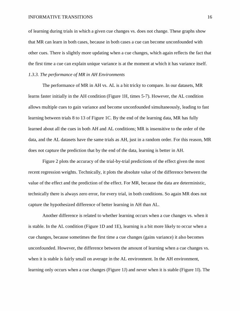
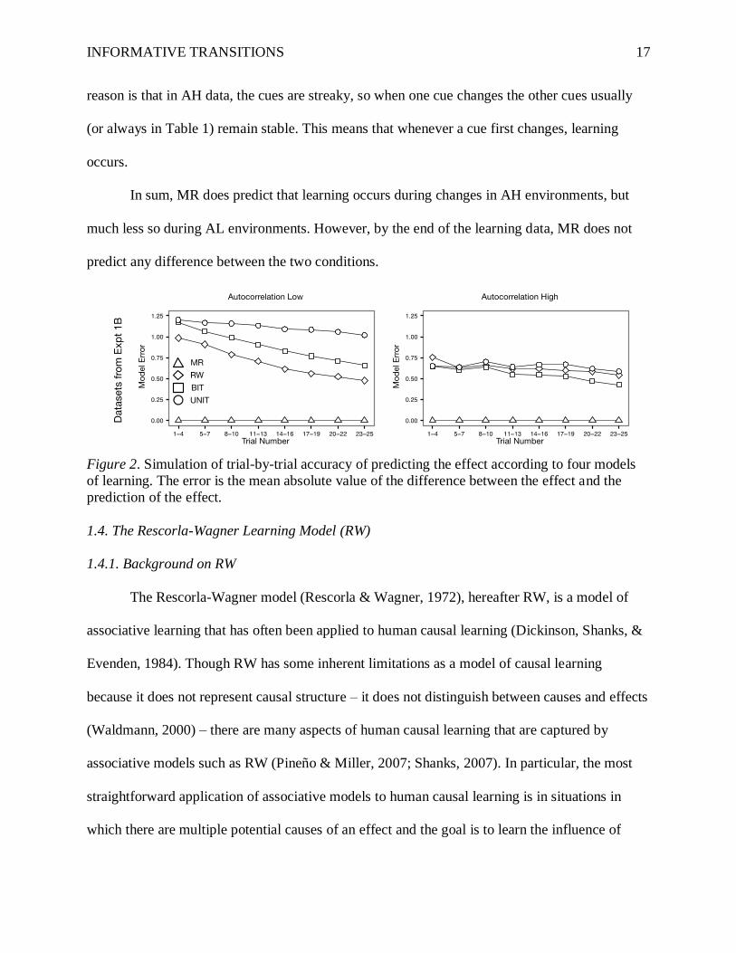
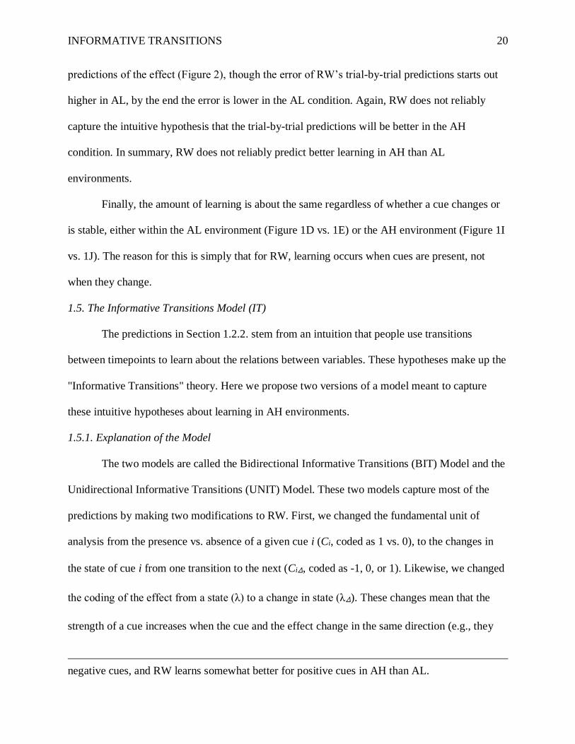
Figure 2 plots the accuracy of the trial-by-trial predictions of the effect given the most
recent regression weights. Technically, it plots the absolute value of the difference between the
value of the effect and the prediction of the effect. For MR, because the data are deterministic,
technically there is always zero error, for every trial, in both conditions. So again MR does not
capture the hypothesized difference of better learning in AH than AL.
Another difference is related to whether learning occurs when a cue changes vs. when it
is stable. In the AL condition (Figure 1D and 1E), learning is a bit more likely to occur when a
cue changes, because sometimes the first time a cue changes (gains variance) it also becomes
unconfounded. However, the difference between the amount of learning when a cue changes vs.
when it is stable is fairly small on average in the AL environment. In the AH environment,
learning only occurs when a cue changes (Figure 1J) and never when it is stable (Figure 1I). The
INFORMATIVE TRANSITIONS 17
reason is that in AH data, the cues are streaky, so when one cue changes the other cues usually
(or always in Table 1) remain stable. This means that whenever a cue first changes, learning
occurs.
In sum, MR does predict that learning occurs during changes in AH environments, but
much less so during AL environments. However, by the end of the learning data, MR does not
predict any difference between the two conditions.
Figure 2. Simulation of trial-by-trial accuracy of predicting the effect according to four models
of learning. The error is the mean absolute value of the difference between the effect and the
prediction of the effect.
1.4. The Rescorla-Wagner Learning Model (RW)
1.4.1. Background on RW
The Rescorla-Wagner model (Rescorla & Wagner, 1972), hereafter RW, is a model of
associative learning that has often been applied to human causal learning (Dickinson, Shanks, &
Evenden, 1984). Though RW has some inherent limitations as a model of causal learning
because it does not represent causal structure – it does not distinguish between causes and effects
(Waldmann, 2000) – there are many aspects of human causal learning that are captured by
associative models such as RW (Pineño & Miller, 2007; Shanks, 2007). In particular, the most
straightforward application of associative models to human causal learning is in situations in
which there are multiple potential causes of an effect and the goal is to learn the influence of
INFORMATIVE TRANSITIONS 18
each of these cues. In the long run, under many standard paradigms, RW calculates ‘conditional
contrasts’ for each cue, which means that it estimates the strength of a cue while controlling for
alternative cues that could be confounded with the target cue, similar to multiple regression
(Cheng, 1997; Danks, 2003).
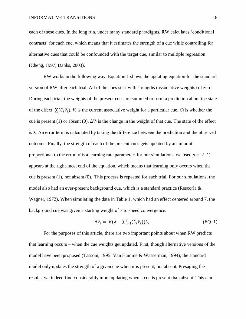
RW works in the following way. Equation 1 shows the updating equation for the standard
version of RW after each trial. All of the cues start with strengths (associative weights) of zero.
During each trial, the weights of the present cues are summed to form a prediction about the state
of the effect: ∑(𝐶𝑖𝑉𝑖). Vi is the current associative weight for a particular cue. Ci is whether the
cue is present (1) or absent (0). ∆Vi is the change in the weight of that cue. The state of the effect
is λ. An error term is calculated by taking the difference between the prediction and the observed
outcome. Finally, the strength of each of the present cues gets updated by an amount
proportional to the error. β is a learning rate parameter; for our simulations, we used β = .2. Ci
appears at the right-most end of the equation, which means that learning only occurs when the
cue is present (1), not absent (0). This process is repeated for each trial. For our simulations, the
model also had an ever-present background cue, which is a standard practice (Rescorla &
Wagner, 1972). When simulating the data in Table 1, which had an effect centered around 7, the
background cue was given a starting weight of 7 to speed convergence.
∆𝑉𝑖 = 𝛽( − ∑ (𝐶𝑖𝑉𝑖))𝐶𝑖8𝑖=1 (EQ. 1)
For the purposes of this article, there are two important points about when RW predicts
that learning occurs – when the cue weights get updated. First, though alternative versions of the
model have been proposed (Tassoni, 1995; Van Hamme & Wasserman, 1994), the standard
model only updates the strength of a given cue when it is present, not absent. Presaging the
results, we indeed find considerably more updating when a cue is present than absent. This can
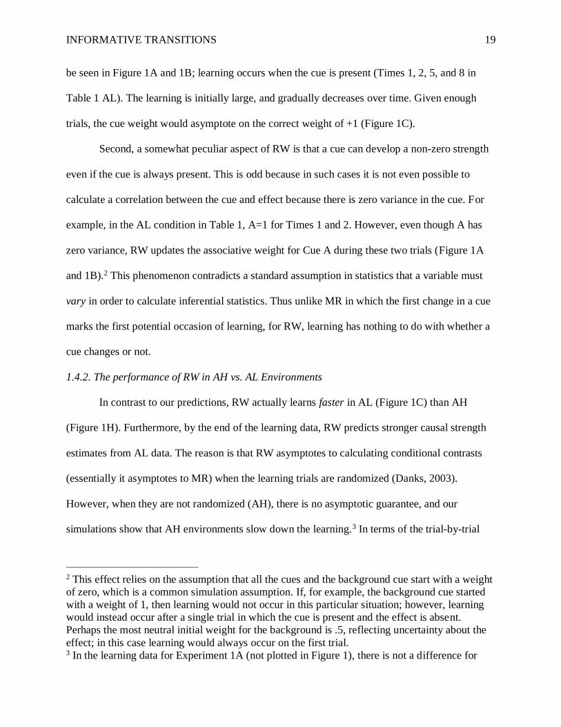
INFORMATIVE TRANSITIONS 19
be seen in Figure 1A and 1B; learning occurs when the cue is present (Times 1, 2, 5, and 8 in
Table 1 AL). The learning is initially large, and gradually decreases over time. Given enough
trials, the cue weight would asymptote on the correct weight of +1 (Figure 1C).
Second, a somewhat peculiar aspect of RW is that a cue can develop a non-zero strength
even if the cue is always present. This is odd because in such cases it is not even possible to
calculate a correlation between the cue and effect because there is zero variance in the cue. For
example, in the AL condition in Table 1, A=1 for Times 1 and 2. However, even though A has
zero variance, RW updates the associative weight for Cue A during these two trials (Figure 1A
and 1B).2 This phenomenon contradicts a standard assumption in statistics that a variable must
vary in order to calculate inferential statistics. Thus unlike MR in which the first change in a cue
marks the first potential occasion of learning, for RW, learning has nothing to do with whether a
cue changes or not.
1.4.2. The performance of RW in AH vs. AL Environments
In contrast to our predictions, RW actually learns faster in AL (Figure 1C) than AH
(Figure 1H). Furthermore, by the end of the learning data, RW predicts stronger causal strength
estimates from AL data. The reason is that RW asymptotes to calculating conditional contrasts
(essentially it asymptotes to MR) when the learning trials are randomized (Danks, 2003).
However, when they are not randomized (AH), there is no asymptotic guarantee, and our
simulations show that AH environments slow down the learning.3 In terms of the trial-by-trial
2 This effect relies on the assumption that all the cues and the background cue start with a weight
of zero, which is a common simulation assumption. If, for example, the background cue started
with a weight of 1, then learning would not occur in this particular situation; however, learning
would instead occur after a single trial in which the cue is present and the effect is absent.
Perhaps the most neutral initial weight for the background is .5, reflecting uncertainty about the
effect; in this case learning would always occur on the first trial. 3 In the learning data for Experiment 1A (not plotted in Figure 1), there is not a difference for
INFORMATIVE TRANSITIONS 20
predictions of the effect (Figure 2), though the error of RW’s trial-by-trial predictions starts out
higher in AL, by the end the error is lower in the AL condition. Again, RW does not reliably
capture the intuitive hypothesis that the trial-by-trial predictions will be better in the AH
condition. In summary, RW does not reliably predict better learning in AH than AL
environments.
Finally, the amount of learning is about the same regardless of whether a cue changes or
is stable, either within the AL environment (Figure 1D vs. 1E) or the AH environment (Figure 1I
vs. 1J). The reason for this is simply that for RW, learning occurs when cues are present, not
when they change.
1.5. The Informative Transitions Model (IT)
The predictions in Section 1.2.2. stem from an intuition that people use transitions
between timepoints to learn about the relations between variables. These hypotheses make up the
"Informative Transitions" theory. Here we propose two versions of a model meant to capture
these intuitive hypotheses about learning in AH environments.
1.5.1. Explanation of the Model
The two models are called the Bidirectional Informative Transitions (BIT) Model and the
Unidirectional Informative Transitions (UNIT) Model. These two models capture most of the
predictions by making two modifications to RW. First, we changed the fundamental unit of
analysis from the presence vs. absence of a given cue i (Ci, coded as 1 vs. 0), to the changes in
the state of cue i from one transition to the next (Ci∆, coded as -1, 0, or 1). Likewise, we changed
the coding of the effect from a state (λ) to a change in state (λ∆). These changes mean that the
strength of a cue increases when the cue and the effect change in the same direction (e.g., they
negative cues, and RW learns somewhat better for positive cues in AH than AL.
INFORMATIVE TRANSITIONS 21
both change from absent to present or vice versa), and the strength of a cue decreases when the
cue and the effect change in opposite directions. This difference also means that no learning
occurs when a cue stays constant.
The second difference is in the amount of updating. For RW, regardless of how many
cues are present, RW updates them all by the same amount. In Section 1.2.2. we suggested that
individuals might learn more during a one-change transition than during a multi-change
transition. We implemented this in Equation 2 by dividing the updating amount by the number of
cues that changed during the transition (η).
∆𝑉𝑖 =𝛽(𝜆∆− ∑ (𝐶𝑖∆𝑉𝑖))𝐶𝑖∆
8𝑖=1
𝜂 (EQ. 2)
The difference between BIT vs. UNIT is that BIT updates the causal strengths when a cue
turns on (from 0 to 1) or off (from 1 to 0), whereas UNIT only updates the causal strengths when
a cue turns on. BIT was our first attempt at a model and is the simplest version of a transitions-
based model. We created UNIT for a couple of reasons. RW predicts that learning occurs when a
cue is present, not absent, and indeed we found evidence of this effect, which can be captured to
some extent by assuming that learning occurs primarily when a cue turns on. Second, UNIT is
actually very similar to a reinforcement learning model developed by Klopf (1988) called the
Drive-Reinforcement model. According to this model, learning occurs when a cue turns on and
the effect changes. The Drive-Reinforcement model is considerably more complicated in ways
that are inspired by neural assumptions that are overly restrictive for our purposes. It is also built
for real-time classical conditioning paradigms and is challenging to use as a model of a self-
paced, trial-by-trial human learning paradigm. For these reasons, we chose to propose UNIT
instead of using Klopf’s model to demonstrate the minimal modifications that need to be made
relative to RW to accommodate our findings. Algorithmically, this is achieved by modifying

INFORMATIVE TRANSITIONS 22
Equation 2 by multiplying the amount of updating by the state of the cue after the transition (i.e.,
1 if the cue turns on, 0 if it turns off).
1.5.2. Simulations of BIT and UNIT.
BIT and UNIT both capture many of the intuitive predictions from Section 1.2.2. This
section goes through each of the predictions. There are a few instances in which the model
captures the data for Experiment 1B (Figure 1) but not for Experiment 1A (binary effect data), or
vice versa, which are noted below.
The most basic hypothesis is that individuals are likely to update their beliefs about
causal strength when the cue changes in either direction (BIT) or changes from 0 to 1 (UNIT).
This can be seen in Figure 1. In the AL data in Table 1 (also Figure 1A and 1B), Time 3 is the
first time that Cue A changes, and is the first time that BIT exhibits learning. BIT only learns a
little because five other cues change simultaneously. Since A changes from 1 to 0 at Time 3,
UNIT does not learn; it first learns at Time 5 when A changes from 0 to 1. In the AH data (also
Figure 1F and 1G), both BIT and UNIT first learn at Time 4 when Cue A changes from 0 to 1.
When looking at the aggregated data across all the learning datasets, for both BIT and UNIT, the
weights are only updated when the cues change (Figure 1E and 1J), not then they are stable
(Figure 1D and 1I).
In addition, according to BIT and UNIT, causal strength beliefs are updated more during
a one-change transition, when only one cue changes and all the other cues remain stable, relative
to a multi-change transition, when two or more cues change simultaneously. This is the reason
that the amount of learning is higher for BIT and UNIT in Figure 1J (AH data; only one cue
changes at a time) than in Figure 1E (AL data; multiple cues change simultaneously); note the
differences in the Y axis.
INFORMATIVE TRANSITIONS 23
Another hypothesis concerns subjects’ final causal strength judgments in AH vs. AL
environments. If people focus on changes, they will learn better in environments with high vs.
low autocorrelation, because there are many one-change transitions in the AH condition but
predominantly multi-change transitions in the AL condition. Multi-change transitions can lead to
incorrect learning. For example, if a positive cue and a neutral cue both turn on simultaneously,
the effect will increase, and that increase could be attributed to both cues or either one. (BIT and
UNIT would update both cues in a positive direction.) This can be seen in the fact that BIT
asymptotes a bit higher in Figure 1H than 1C. UNIT actually fails to capture this prediction in
the Experiment 1B data in Figure 14, though it does for the Experiment 1A data.
A related hypothesis is that if subjects do not learn as well in the AL condition compared
to the AH condition, then their trial-by-trial predictions of the effect should be less accurate.
Indeed, in Figure 2, both BIT and UNIT have lower error in the trial-by-trial predictions of the
effect in AH than AL environments. However, none of the models capture this hypothesis for the
Experiment 1A datasets; see Section 2.2.3 for more details.
In sum both BIT and UNIT capture most of the predictions proposed in Section 1.2.2.
Further analyses will reveal whether people primarily update whenever a cue changes (BIT) or
primarily when a cue turns on (UNIT).
1.6. Outline of Experiments
In Experiments 1A and 1B, we tested whether, by the end of the learning data,
participants develop more accurate estimates of causal influence in an environment in which the
cues are fairly stable and only one cue changes at a time (AH), compared to an environment in
4 UNIT learns about as much in AL (Figure 1C) and AH (Figure 1H). The reason essentially is
that in AL relative to AH there are more changes and therefore more opportunities to learn, but
learning is slowed down because multiple cues change simultaneously. For UNIT both of these
factors roughly cancel out, whereas for BIT the second dominates.
INFORMATIVE TRANSITIONS 24
which the trials are randomly presented and often multiple cues change from one observation to
the next (AL). These experiments also allowed us to test whether subjects are more likely to
update their beliefs about causal strength when a cue changes vs. does not change. In Experiment
2, we tested whether participants are more likely to update their beliefs about the influence of a
cue, trial-by-trial, when only one cue changes relative to two or three cues changing, all within
an AH environment.
In Experiments 3 and 4, we tested the implications of learning about cues in
environments in which the order of the learning trials is organized in two different ways.
Intuitively it may be easier to learn causal relations if the data are organized in ways that makes
it easier to summarize the trials, such as organizing the trials by the state of the effect
(Experiment 3) or organizing the trials by the states of the cues (Experiment 4). However,
organizing the trials in these ways reduces the number of one-change transitions, which could
impair learning according to the IT models.
2. Experiment 1A: Learning with a Binary Effect
In Experiment 1A, we manipulated the order of the data participants experienced to
determine if participants would learn better in an AH vs. AL environment. The effect was a
binary variable. (See Table 2 for an example.) In the AH condition, every transition was a one-
change transition, whereas in the AL condition, the trial order from the AH condition was
randomized, which is a common feature of many trial-by-trial causal and associative learning
studies (e.g., Busemeyer, Myung, & McDaniel, 1993; Goedert & Spellman, 2005; Spellman et
al., 2001). A random trial order means that frequently multiple cues changed simultaneously.
Because the same trials were used across the two conditions, the final multiple regression outputs
and bivariate correlations are the same for the two conditions (Table 3).
INFORMATIVE TRANSITIONS 25
2.1. Method
2.1.1. Participants
For all the experiments in the article, participants were recruited using Amazon’s
Mechanical Turk service (MTurk). Only participants in the US with an acceptance rate of over
95% were eligible for the experiments. We also limited the sample to participants who had not
completed any other experiment in this study. In Experiment 1A, 100 participants were recruited.
They were paid $2 for Experiments 1A and 1B (approximately $6-$8 per hour) plus a bonus
described below.
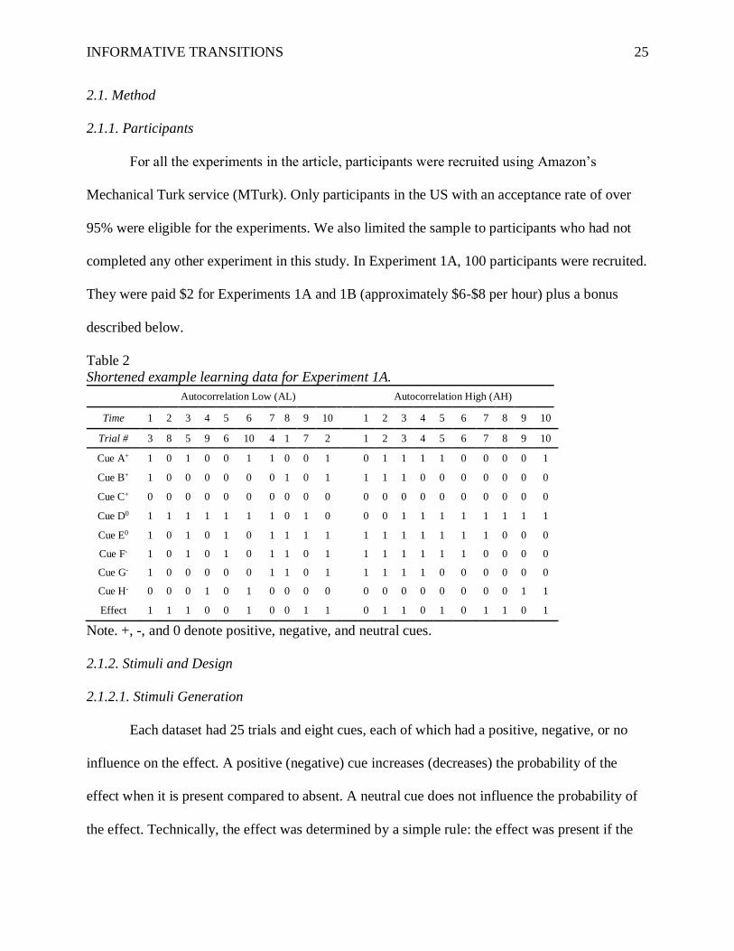
Table 2
Shortened example learning data for Experiment 1A.
Autocorrelation Low (AL) Autocorrelation High (AH)
Time 1 2 3 4 5 6 7 8 9 10 1 2 3 4 5 6 7 8 9 10
Trial # 3 8 5 9 6 10 4 1 7 2 1 2 3 4 5 6 7 8 9 10
Cue A+ 1 0 1 0 0 1 1 0 0 1 0 1 1 1 1 0 0 0 0 1
Cue B+ 1 0 0 0 0 0 0 1 0 1 1 1 1 0 0 0 0 0 0 0
Cue C+ 0 0 0 0 0 0 0 0 0 0 0 0 0 0 0 0 0 0 0 0
Cue D0 1 1 1 1 1 1 1 0 1 0 0 0 1 1 1 1 1 1 1 1
Cue E0 1 0 1 0 1 0 1 1 1 1 1 1 1 1 1 1 1 0 0 0
Cue F- 1 0 1 0 1 0 1 1 0 1 1 1 1 1 1 1 0 0 0 0
Cue G- 1 0 0 0 0 0 1 1 0 1 1 1 1 1 0 0 0 0 0 0
Cue H- 0 0 0 1 0 1 0 0 0 0 0 0 0 0 0 0 0 0 1 1
Effect 1 1 1 0 0 1 0 0 1 1 0 1 1 0 1 0 1 1 0 1
Note. +, -, and 0 denote positive, negative, and neutral cues.
2.1.2. Stimuli and Design
2.1.2.1. Stimuli Generation
Each dataset had 25 trials and eight cues, each of which had a positive, negative, or no
influence on the effect. A positive (negative) cue increases (decreases) the probability of the
effect when it is present compared to absent. A neutral cue does not influence the probability of
the effect. Technically, the effect was determined by a simple rule: the effect was present if the
INFORMATIVE TRANSITIONS 26
number of positive cues that were present on a given trial was greater than or equal to the
number of negative cues.
Because participants worked with three datasets, we systematically varied the number of
positive, negative, and neutral cues in each dataset to prevent participants from knowing how
many of each to expect. There were three types of datasets: datasets with two positive cues (and
three negative and three neutral), two negative (and three positive and three neutral), or two
neutral (and three positive and three negative). (Table 2 is an example with three positive, three
negative, and two neutral cues.) The different types of datasets were not separated for analysis.
Datasets for the AH condition were generated in the following way; see Table 2 for a
shortened example. Each of the eight cues changed three times, and each time it changed all
other cues remained stable (one-change transitions), resulting in 24 total transitions (25 trials).
For the first trial, the states of the eight cues and the effect were determined randomly. On each
subsequent trial, one of the eight cues was chosen to change relative to the prior trial. Neutral
cues could always be selected to change, provided they had not yet changed three times. Positive
and negative cues were only eligible to be selected to change under certain conditions. Positive
cues could only change if they were in the same state as the effect; for a positive cue to change
from 0 to 1, the effect had to initially be 0 so that it could change to 1. If the effect was initially
at 1, then even if the positive cue changed to 1, the effect would not be able to change. The same
is true in reverse for negative cues, which could only change when they were in the opposite
state as the effect. One hundred fifty datasets for the AH condition were created with a computer
program.
INFORMATIVE TRANSITIONS 27
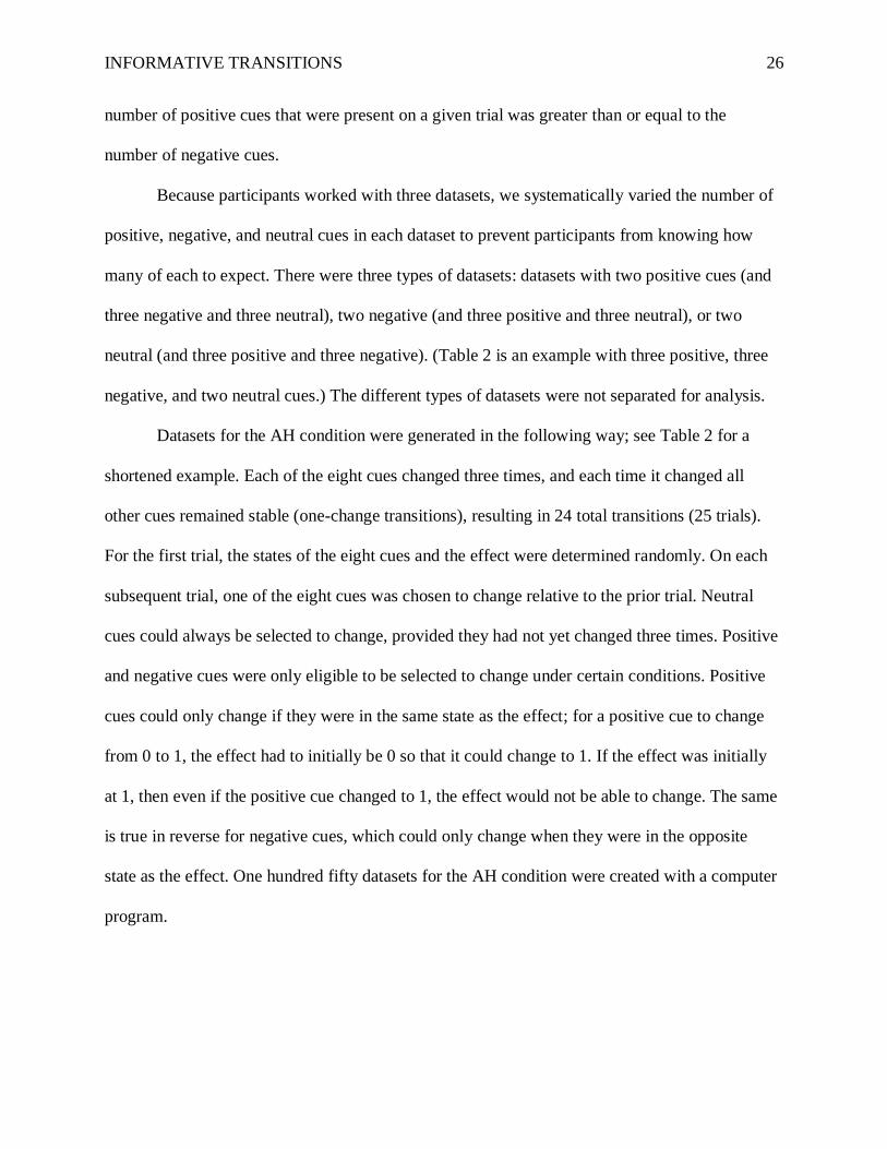
Table 3
Average bivariate and multivariate partial r2 for positive, negative, and neutral cues for datasets
in each experiment
Experiments 1A & 3 Experiments 1B, 2, & 4
Valence Bivariate r2 Multivariate
Partial r2 Bivariate r2
Multivariate
Partial r2
Positive/Negative 0.07 1.00 0.24 1.00
Neutral 0.02 0.00 0.10 0.00
The datasets for the AL condition were the same datasets from the AH condition, except
that the trials were presented to participants in a randomized order; the randomization occurred
separately for each participant and dataset.
2.1.2.2. Stimuli Properties
Creating the datasets in this way produced a number of important characteristics. First,
the positive and negative cues are perfectly predictive. Within a dataset, it is possible to perfectly
predict the effect from the eight cues; multiple r2=1. This also means that each of the positive
and negative cues, controlling for the other seven, perfectly predicts the effect, so the partial
variance explained is 100% for the positive and negative cues (Table 3). Thus, if participants
control for alternative cues, they should judge the positive and negative cues to be very strong. In
contrast, the average variance explained by a single cue, not controlling for the others was just
7% (Table 3; Bivariate r2).
Second, both logistic and linear regression fit the data perfectly. For logistic regression,
the weights would approach positive infinity, zero, and negative infinity for the positive, neutral,
and negative cues. For linear regression, the weights are exactly +1, 0, and -1 for the positive,
neutral, and negative cues. Instead of regression weights, we focus on partial variance explained
by each of the eight cues. Unlike regression weights, partial variance explained has the same
meaning in logistic and linear regression; linear regression is necessary for Experiment 1B.
Partial variance explained is also bounded, and because the cues perfectly predict the outcome, a

INFORMATIVE TRANSITIONS 28
partial variance explained approach argues that the positive and negative explain 100% of the
remaining variance.
Third, if multiple regression is performed after each trial, as soon as a regression weight
can be calculated (the cue has variance and is not perfectly confounded with another cue), the
regression weight and the partial variance explained goes right to the correct value (i.e., +1 linear
regression weight, 100% partial variance explained for a positive cue).
Fourth, the cues do not interact with each other. If a multiple regression is run with all
eight cues as well as all possible interactions, all of the interactions have a weight of zero (unless
they are confounded with one of the cues, in which the cues were given precedence and the
interaction was ignored). This feature is true even if the regression is run after each trial, and for
both logistic and linear regression. In sum, there is no need to posit any interactions because
main effects perfectly explain the causal relations.
Lastly, although Figures 1 and 2 present simulations of the datasets in Experiment 1B
which use an effect on a continuous scale, simulations using the datasets in Experiment 1A with
a binary effect show mostly the same patterns except where previously noted.
2.1.3. Procedure
Participants were randomly assigned to either the AH or AL condition, between subjects,
and worked with three datasets. One dataset of each of the three types was randomly selected,
and the order of these three was randomized.
Participants were asked to imagine that they worked for a nursing home, and that their
job was to determine if the medications (cues) the patients were taking influenced the quality of
their sleep (effect). After completing a brief practice dataset with 7 trials in which every
transition was one-change, participants began the experiment. Each of the three datasets was
INFORMATIVE TRANSITIONS 29
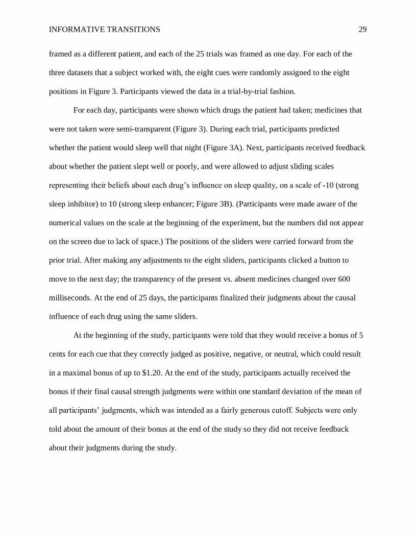
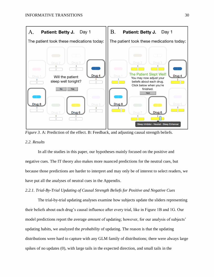
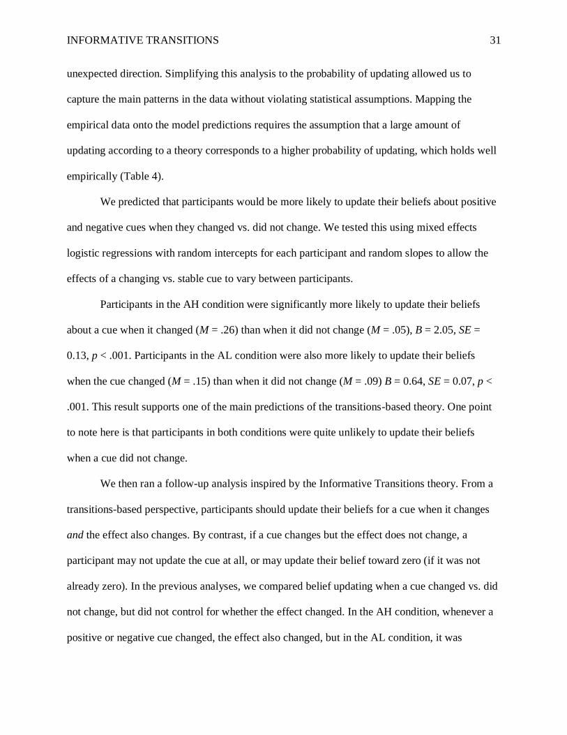
framed as a different patient, and each of the 25 trials was framed as one day. For each of the
three datasets that a subject worked with, the eight cues were randomly assigned to the eight
positions in Figure 3. Participants viewed the data in a trial-by-trial fashion.
For each day, participants were shown which drugs the patient had taken; medicines that
were not taken were semi-transparent (Figure 3). During each trial, participants predicted
whether the patient would sleep well that night (Figure 3A). Next, participants received feedback
about whether the patient slept well or poorly, and were allowed to adjust sliding scales
representing their beliefs about each drug’s influence on sleep quality, on a scale of -10 (strong
sleep inhibitor) to 10 (strong sleep enhancer; Figure 3B). (Participants were made aware of the
numerical values on the scale at the beginning of the experiment, but the numbers did not appear
on the screen due to lack of space.) The positions of the sliders were carried forward from the
prior trial. After making any adjustments to the eight sliders, participants clicked a button to
move to the next day; the transparency of the present vs. absent medicines changed over 600
milliseconds. At the end of 25 days, the participants finalized their judgments about the causal
influence of each drug using the same sliders.
At the beginning of the study, participants were told that they would receive a bonus of 5
cents for each cue that they correctly judged as positive, negative, or neutral, which could result
in a maximal bonus of up to $1.20. At the end of the study, participants actually received the
bonus if their final causal strength judgments were within one standard deviation of the mean of
all participants’ judgments, which was intended as a fairly generous cutoff. Subjects were only
told about the amount of their bonus at the end of the study so they did not receive feedback
about their judgments during the study.
INFORMATIVE TRANSITIONS 30
Figure 3. A: Prediction of the effect. B: Feedback, and adjusting causal strength beliefs.
2.2. Results
In all the studies in this paper, our hypotheses mainly focused on the positive and
negative cues. The IT theory also makes more nuanced predictions for the neutral cues, but
because those predictions are harder to interpret and may only be of interest to select readers, we
have put all the analyses of neutral cues in the Appendix.
2.2.1. Trial-By-Trial Updating of Causal Strength Beliefs for Positive and Negative Cues
The trial-by-trial updating analyses examine how subjects update the sliders representing
their beliefs about each drug’s causal influence after every trial, like in Figure 1B and 1G. Our
model predictions report the average amount of updating; however, for our analysis of subjects’
updating habits, we analyzed the probability of updating. The reason is that the updating
distributions were hard to capture with any GLM family of distributions; there were always large
spikes of no updates (0), with large tails in the expected direction, and small tails in the
INFORMATIVE TRANSITIONS 31
unexpected direction. Simplifying this analysis to the probability of updating allowed us to
capture the main patterns in the data without violating statistical assumptions. Mapping the
empirical data onto the model predictions requires the assumption that a large amount of
updating according to a theory corresponds to a higher probability of updating, which holds well
empirically (Table 4).
We predicted that participants would be more likely to update their beliefs about positive
and negative cues when they changed vs. did not change. We tested this using mixed effects
logistic regressions with random intercepts for each participant and random slopes to allow the
effects of a changing vs. stable cue to vary between participants.
Participants in the AH condition were significantly more likely to update their beliefs
about a cue when it changed (M = .26) than when it did not change (M = .05), B = 2.05, SE =
0.13, p < .001. Participants in the AL condition were also more likely to update their beliefs
when the cue changed (M = .15) than when it did not change (M = .09) B = 0.64, SE = 0.07, p <
.001. This result supports one of the main predictions of the transitions-based theory. One point
to note here is that participants in both conditions were quite unlikely to update their beliefs
when a cue did not change.
We then ran a follow-up analysis inspired by the Informative Transitions theory. From a
transitions-based perspective, participants should update their beliefs for a cue when it changes
and the effect also changes. By contrast, if a cue changes but the effect does not change, a
participant may not update the cue at all, or may update their belief toward zero (if it was not
already zero). In the previous analyses, we compared belief updating when a cue changed vs. did
not change, but did not control for whether the effect changed. In the AH condition, whenever a
positive or negative cue changed, the effect also changed, but in the AL condition, it was
INFORMATIVE TRANSITIONS 32
possible for multiple cues to change but the effect not to change. Furthermore, in the AH
condition, when a cue did not change, it was possible for 1) another positive or negative cue to
change, in which case the effect also changed, or 2) for a ‘neutral’ causal to change, in which
case the effect did not change.
To develop a closer comparison within and across conditions, we ran the following
analyses within the subset of trials in which the effect changed. First, within the AH condition,
participants were more likely to update their beliefs about a given cue when that cue changed (M
= .26) than when the cue did not change (M = .05), B = 2.04, SE = 0.14, p < .001. Second, in the
AL condition, participants were also more likely to update their beliefs about a given cue when
that cue changed (M = .17) than when the cue did not change (M = .09), B = 0.72, SE = 0.09, p <
.001. Third, participants were more likely to update their beliefs about a given cue in the AH
condition when that cue changed (and no other cues changed) than in the AL condition, when a
given cue changed (and other cues may have also changed) B = -0.63, SE = 0.16, p < .001. This
last finding is evidence that participants are more likely to update their beliefs during a ‘one-
change’ transition.
For simplicity and consistency, all further trial-by-trial analyses of causal strength belief
updating will be reported for the subset of data in which the effect changed. None of the
significance tests were changed by subsetting the data in this way.
Table 4 reports these statistics of the probability of updating when the cue changes vs.
does not change, and the effect changes, for all experiments. A visual summary of the empirical
results and the predictions from each model is provided in Figure 4. (See Section 7 for a
discussion of qualitative model predictions.)
INFORMATIVE TRANSITIONS 33
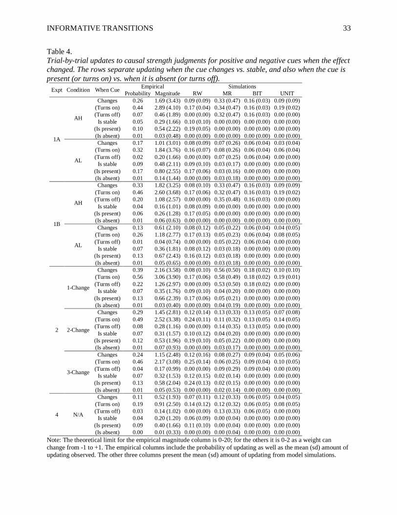
Table 4.
Trial-by-trial updates to causal strength judgments for positive and negative cues when the effect
changed. The rows separate updating when the cue changes vs. stable, and also when the cue is
present (or turns on) vs. when it is absent (or turns off).
Expt Condition When Cue Empirical Simulations
Probability Magnitude RW MR BIT UNIT
1A
AH
Changes 0.26 1.69 (3.43) 0.09 (0.09) 0.33 (0.47) 0.16 (0.03) 0.09 (0.09)
(Turns on) 0.44 2.89 (4.10) 0.17 (0.04) 0.34 (0.47) 0.16 (0.03) 0.19 (0.02)
(Turns off) 0.07 0.46 (1.89) 0.00 (0.00) 0.32 (0.47) 0.16 (0.03) 0.00 (0.00)
Is stable 0.05 0.29 (1.66) 0.10 (0.10) 0.00 (0.00) 0.00 (0.00) 0.00 (0.00)
(Is present) 0.10 0.54 (2.22) 0.19 (0.05) 0.00 (0.00) 0.00 (0.00) 0.00 (0.00)
(Is absent) 0.01 0.03 (0.48) 0.00 (0.00) 0.00 (0.00) 0.00 (0.00) 0.00 (0.00)
AL
Changes 0.17 1.01 (3.01) 0.08 (0.09) 0.07 (0.26) 0.06 (0.04) 0.03 (0.04)
(Turns on) 0.32 1.84 (3.76) 0.16 (0.07) 0.08 (0.26) 0.06 (0.04) 0.06 (0.04)
(Turns off) 0.02 0.20 (1.66) 0.00 (0.00) 0.07 (0.25) 0.06 (0.04) 0.00 (0.00)
Is stable 0.09 0.48 (2.11) 0.09 (0.10) 0.03 (0.17) 0.00 (0.00) 0.00 (0.00)
(Is present) 0.17 0.80 (2.55) 0.17 (0.06) 0.03 (0.16) 0.00 (0.00) 0.00 (0.00)
(Is absent) 0.01 0.14 (1.44) 0.00 (0.00) 0.03 (0.18) 0.00 (0.00) 0.00 (0.00)
1B
AH
Changes 0.33 1.82 (3.25) 0.08 (0.10) 0.33 (0.47) 0.16 (0.03) 0.09 (0.09)
(Turns on) 0.46 2.60 (3.68) 0.17 (0.06) 0.32 (0.47) 0.16 (0.03) 0.19 (0.02)
(Turns off) 0.20 1.08 (2.57) 0.00 (0.00) 0.35 (0.48) 0.16 (0.03) 0.00 (0.00)
Is stable 0.04 0.16 (1.01) 0.08 (0.09) 0.00 (0.00) 0.00 (0.00) 0.00 (0.00)
(Is present) 0.06 0.26 (1.28) 0.17 (0.05) 0.00 (0.00) 0.00 (0.00) 0.00 (0.00)
(Is absent) 0.01 0.06 (0.63) 0.00 (0.00) 0.00 (0.00) 0.00 (0.00) 0.00 (0.00)
AL
Changes 0.13 0.61 (2.10) 0.08 (0.12) 0.05 (0.22) 0.06 (0.04) 0.04 (0.05)
(Turns on) 0.26 1.18 (2.77) 0.17 (0.13) 0.05 (0.23) 0.06 (0.04) 0.08 (0.05)
(Turns off) 0.01 0.04 (0.74) 0.00 (0.00) 0.05 (0.22) 0.06 (0.04) 0.00 (0.00)
Is stable 0.07 0.36 (1.81) 0.08 (0.12) 0.03 (0.18) 0.00 (0.00) 0.00 (0.00)
(Is present) 0.13 0.67 (2.43) 0.16 (0.12) 0.03 (0.18) 0.00 (0.00) 0.00 (0.00)
(Is absent) 0.01 0.05 (0.65) 0.00 (0.00) 0.03 (0.18) 0.00 (0.00) 0.00 (0.00)
2
1-Change
Changes 0.39 2.16 (3.58) 0.08 (0.10) 0.56 (0.50) 0.18 (0.02) 0.10 (0.10)
(Turns on) 0.56 3.06 (3.90) 0.17 (0.06) 0.58 (0.49) 0.18 (0.02) 0.19 (0.01)
(Turns off) 0.22 1.26 (2.97) 0.00 (0.00) 0.53 (0.50) 0.18 (0.02) 0.00 (0.00)
Is stable 0.07 0.35 (1.76) 0.09 (0.10) 0.04 (0.20) 0.00 (0.00) 0.00 (0.00)
(Is present) 0.13 0.66 (2.39) 0.17 (0.06) 0.05 (0.21) 0.00 (0.00) 0.00 (0.00)
(Is absent) 0.01 0.03 (0.40) 0.00 (0.00) 0.04 (0.19) 0.00 (0.00) 0.00 (0.00)
2-Change
Changes 0.29 1.45 (2.81) 0.12 (0.14) 0.13 (0.33) 0.13 (0.05) 0.07 (0.08)
(Turns on) 0.49 2.52 (3.38) 0.24 (0.11) 0.11 (0.32) 0.13 (0.05) 0.14 (0.05)
(Turns off) 0.08 0.28 (1.16) 0.00 (0.00) 0.14 (0.35) 0.13 (0.05) 0.00 (0.00)
Is stable 0.07 0.31 (1.57) 0.10 (0.12) 0.04 (0.20) 0.00 (0.00) 0.00 (0.00)
(Is present) 0.12 0.53 (1.96) 0.19 (0.10) 0.05 (0.22) 0.00 (0.00) 0.00 (0.00)
(Is absent) 0.01 0.07 (0.93) 0.00 (0.00) 0.03 (0.17) 0.00 (0.00) 0.00 (0.00)
3-Change
Changes 0.24 1.15 (2.48) 0.12 (0.16) 0.08 (0.27) 0.09 (0.04) 0.05 (0.06)
(Turns on) 0.46 2.17 (3.08) 0.25 (0.14) 0.06 (0.25) 0.09 (0.04) 0.10 (0.05)
(Turns off) 0.04 0.17 (0.99) 0.00 (0.00) 0.09 (0.29) 0.09 (0.04) 0.00 (0.00)
Is stable 0.07 0.32 (1.53) 0.12 (0.15) 0.02 (0.14) 0.00 (0.00) 0.00 (0.00)
(Is present) 0.13 0.58 (2.04) 0.24 (0.13) 0.02 (0.15) 0.00 (0.00) 0.00 (0.00)
(Is absent) 0.01 0.05 (0.53) 0.00 (0.00) 0.02 (0.14) 0.00 (0.00) 0.00 (0.00)
4 N/A
Changes 0.11 0.52 (1.93) 0.07 (0.11) 0.12 (0.33) 0.06 (0.05) 0.04 (0.05)
(Turns on) 0.19 0.91 (2.50) 0.14 (0.12) 0.12 (0.32) 0.06 (0.05) 0.08 (0.05)
(Turns off) 0.03 0.14 (1.02) 0.00 (0.00) 0.13 (0.33) 0.06 (0.05) 0.00 (0.00)
Is stable 0.04 0.20 (1.20) 0.06 (0.09) 0.00 (0.04) 0.00 (0.00) 0.00 (0.00)
(Is present) 0.09 0.40 (1.66) 0.11 (0.10) 0.00 (0.04) 0.00 (0.00) 0.00 (0.00)
(Is absent) 0.00 0.01 (0.33) 0.00 (0.00) 0.00 (0.04) 0.00 (0.00) 0.00 (0.00)
Note: The theoretical limit for the empirical magnitude column is 0-20; for the others it is 0-2 as a weight can
change from -1 to +1. The empirical columns include the probability of updating as well as the mean (sd) amount of
updating observed. The other three columns present the mean (sd) amount of updating from model simulations.
INFORMATIVE TRANSITIONS 34
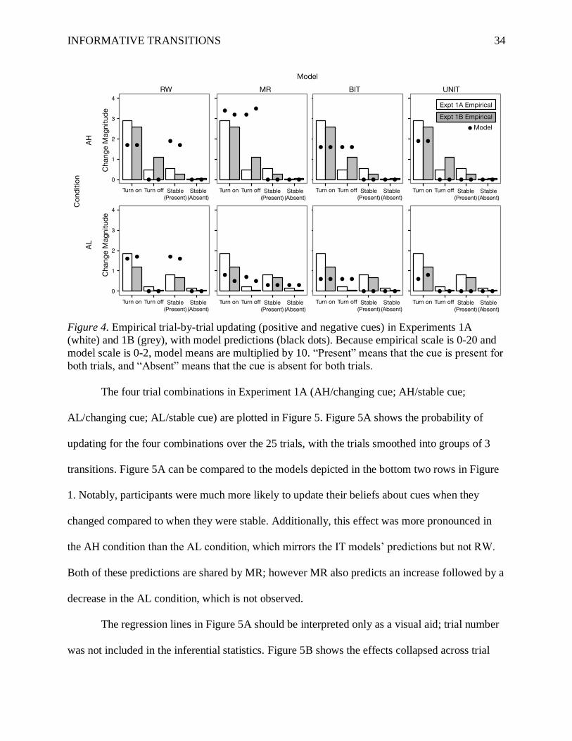
Figure 4. Empirical trial-by-trial updating (positive and negative cues) in Experiments 1A
(white) and 1B (grey), with model predictions (black dots). Because empirical scale is 0-20 and
model scale is 0-2, model means are multiplied by 10. “Present” means that the cue is present for
both trials, and “Absent” means that the cue is absent for both trials.
The four trial combinations in Experiment 1A (AH/changing cue; AH/stable cue;
AL/changing cue; AL/stable cue) are plotted in Figure 5. Figure 5A shows the probability of
updating for the four combinations over the 25 trials, with the trials smoothed into groups of 3
transitions. Figure 5A can be compared to the models depicted in the bottom two rows in Figure
1. Notably, participants were much more likely to update their beliefs about cues when they
changed compared to when they were stable. Additionally, this effect was more pronounced in
the AH condition than the AL condition, which mirrors the IT models’ predictions but not RW.
Both of these predictions are shared by MR; however MR also predicts an increase followed by a
decrease in the AL condition, which is not observed.
The regression lines in Figure 5A should be interpreted only as a visual aid; trial number
was not included in the inferential statistics. Figure 5B shows the effects collapsed across trial
INFORMATIVE TRANSITIONS 35
number. This overall comparison is what we used in the above analyses.
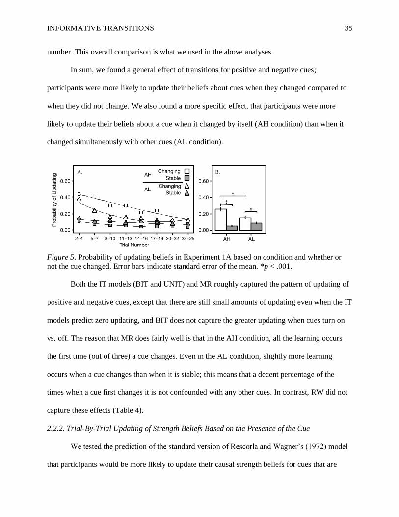
In sum, we found a general effect of transitions for positive and negative cues;
participants were more likely to update their beliefs about cues when they changed compared to
when they did not change. We also found a more specific effect, that participants were more
likely to update their beliefs about a cue when it changed by itself (AH condition) than when it
changed simultaneously with other cues (AL condition).
Figure 5. Probability of updating beliefs in Experiment 1A based on condition and whether or
not the cue changed. Error bars indicate standard error of the mean. *p < .001.
Both the IT models (BIT and UNIT) and MR roughly captured the pattern of updating of
positive and negative cues, except that there are still small amounts of updating even when the IT
models predict zero updating, and BIT does not capture the greater updating when cues turn on
vs. off. The reason that MR does fairly well is that in the AH condition, all the learning occurs
the first time (out of three) a cue changes. Even in the AL condition, slightly more learning
occurs when a cue changes than when it is stable; this means that a decent percentage of the
times when a cue first changes it is not confounded with any other cues. In contrast, RW did not
capture these effects (Table 4).
2.2.2. Trial-By-Trial Updating of Strength Beliefs Based on the Presence of the Cue
We tested the prediction of the standard version of Rescorla and Wagner’s (1972) model
that participants would be more likely to update their causal strength beliefs for cues that are
INFORMATIVE TRANSITIONS 36
present on a given trial than those that are absent. Table 4 separates cues that are present vs.
absent. (For cues that change, the present cues are described as “turning on” and the absent cues
as “turning off”.) As can be seen in Table 4 and Figure 4, there is considerably more updating
when a cue is present than absent for both changing and stable cues.
This effect was formally tested with a mixed effects logistic regression, with
presence/absence of the cue as the predictor. We included by-subject random intercepts and a
random slope for presence/absence of the cue. This analysis included positive, negative, and
neutral cues. Participants were significantly more likely to update their beliefs about cues when
they were present than when they were absent both for the AH condition, (M = .14 vs. .01), B =
2.94, SE = 0.24, p < .001, and for the AL condition, (M = .21 vs. .01), B = 4.21, SE = 0.31, p <
.001. (Note, these summary numbers are not reported in Table 4.) This finding matches
predictions from RW and UNIT, but not BIT. Furthermore, participants in the AL condition were
more likely to update their causal strength beliefs than participants in the AH condition when a
cue was present, B = 0.50, SE = 0.19, p < .01.
In sum, the most updating occurred when a cue turned on, which fits best with the UNIT
model.
2.2.3. Accuracy of Trial-By-Trial Predictions of the Effect
We next analyzed the accuracy of subjects’ trial-by-trial predictions of the effect. For
each trial, participants were shown which medications the patient took that day, and were asked
to predict whether or not the patient would sleep well. We predicted that participants in the AH
condition would be more accurate; if participants are better able to infer causal strength in the
AH condition, they should also be better able to predict the effect. A mixed effects logistic
regression with by-subject random intercepts found that participants were better able to predict
INFORMATIVE TRANSITIONS 37
the effect (i.e. their absolute prediction error was lower) in the AH condition compared to the AL
condition, B = -0.27, SE = 0.07, p < .001. (See Table 5 for descriptive statistics of prediction
error.)
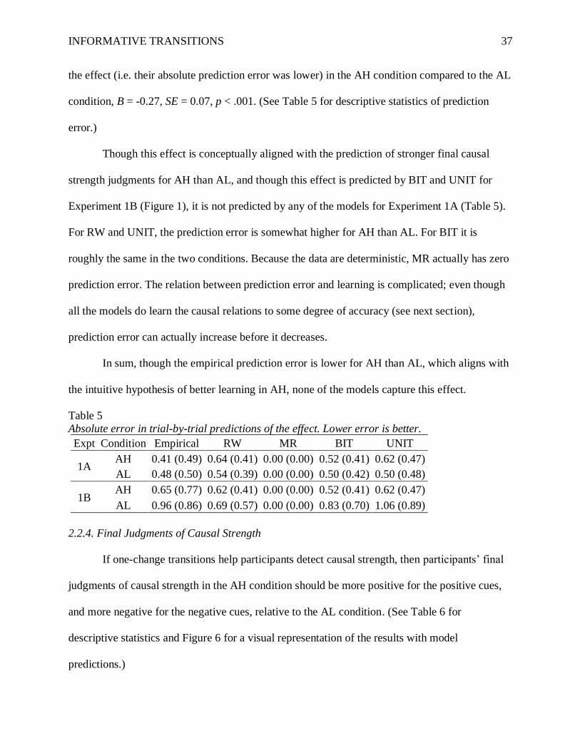
Though this effect is conceptually aligned with the prediction of stronger final causal
strength judgments for AH than AL, and though this effect is predicted by BIT and UNIT for
Experiment 1B (Figure 1), it is not predicted by any of the models for Experiment 1A (Table 5).
For RW and UNIT, the prediction error is somewhat higher for AH than AL. For BIT it is
roughly the same in the two conditions. Because the data are deterministic, MR actually has zero
prediction error. The relation between prediction error and learning is complicated; even though
all the models do learn the causal relations to some degree of accuracy (see next section),
prediction error can actually increase before it decreases.
In sum, though the empirical prediction error is lower for AH than AL, which aligns with
the intuitive hypothesis of better learning in AH, none of the models capture this effect.
Table 5
Absolute error in trial-by-trial predictions of the effect. Lower error is better.
Expt Condition Empirical RW MR BIT UNIT
1A AH 0.41 (0.49) 0.64 (0.41) 0.00 (0.00) 0.52 (0.41) 0.62 (0.47)
AL 0.48 (0.50) 0.54 (0.39) 0.00 (0.00) 0.50 (0.42) 0.50 (0.48)
1B AH 0.65 (0.77) 0.62 (0.41) 0.00 (0.00) 0.52 (0.41) 0.62 (0.47)
AL 0.96 (0.86) 0.69 (0.57) 0.00 (0.00) 0.83 (0.70) 1.06 (0.89)
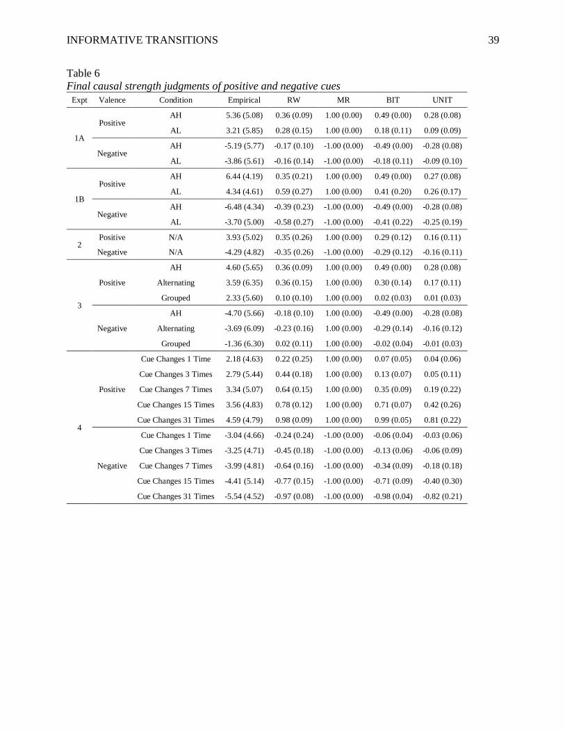
2.2.4. Final Judgments of Causal Strength
If one-change transitions help participants detect causal strength, then participants’ final
judgments of causal strength in the AH condition should be more positive for the positive cues,
and more negative for the negative cues, relative to the AL condition. (See Table 6 for
descriptive statistics and Figure 6 for a visual representation of the results with model
predictions.)

INFORMATIVE TRANSITIONS 38
Because the data were heavily skewed, with many judgments near the positive extreme
for positive cues and the negative extreme for negative cues, we used a Gamma regression. For
positive cues, we transformed the data by multiplying each judgment by -1 and adding 11 so that
the data lay on the positive integers. For negative cues, we added 11 to each judgment. This
meant that ‘stronger’ judgments would be closer to zero. The descriptive statistics are reported
on the original scale. The regression models incorporated a by-subject random intercept and
fixed effect for condition (which was between-Ss). Participants judged the positive cues to be
more positive in the AH condition than in the AL condition (B = -0.07, SE = 0.02, p < .001, R2 =
.03, d = 0.35), and they judged the negative cues to be more negative in the AH condition than
AL condition (B = -0.06, SE = 0.02, p < .01, R2 = .01, d = 0.20).
In respect to the models, MR cannot explain any differences between conditions because
it is insensitive to trial order. RW captured this effect for positive but not negative cues, and not
in subsequent experiments. The IT models captured the directions of the differences between
conditions in Experiment 1A.
INFORMATIVE TRANSITIONS 39
Table 6
Final causal strength judgments of positive and negative cues
Expt Valence Condition Empirical RW MR BIT UNIT
1A
Positive AH 5.36 (5.08) 0.36 (0.09) 1.00 (0.00) 0.49 (0.00) 0.28 (0.08)
AL 3.21 (5.85) 0.28 (0.15) 1.00 (0.00) 0.18 (0.11) 0.09 (0.09)
Negative AH -5.19 (5.77) -0.17 (0.10) -1.00 (0.00) -0.49 (0.00) -0.28 (0.08)
AL -3.86 (5.61) -0.16 (0.14) -1.00 (0.00) -0.18 (0.11) -0.09 (0.10)
1B
Positive AH 6.44 (4.19) 0.35 (0.21) 1.00 (0.00) 0.49 (0.00) 0.27 (0.08)
AL 4.34 (4.61) 0.59 (0.27) 1.00 (0.00) 0.41 (0.20) 0.26 (0.17)
Negative AH -6.48 (4.34) -0.39 (0.23) -1.00 (0.00) -0.49 (0.00) -0.28 (0.08)
AL -3.70 (5.00) -0.58 (0.27) -1.00 (0.00) -0.41 (0.22) -0.25 (0.19)
2 Positive N/A 3.93 (5.02) 0.35 (0.26) 1.00 (0.00) 0.29 (0.12) 0.16 (0.11)
Negative N/A -4.29 (4.82) -0.35 (0.26) -1.00 (0.00) -0.29 (0.12) -0.16 (0.11)
3
Positive
AH 4.60 (5.65) 0.36 (0.09) 1.00 (0.00) 0.49 (0.00) 0.28 (0.08)
Alternating 3.59 (6.35) 0.36 (0.15) 1.00 (0.00) 0.30 (0.14) 0.17 (0.11)
Grouped 2.33 (5.60) 0.10 (0.10) 1.00 (0.00) 0.02 (0.03) 0.01 (0.03)
Negative
AH -4.70 (5.66) -0.18 (0.10) 1.00 (0.00) -0.49 (0.00) -0.28 (0.08)
Alternating -3.69 (6.09) -0.23 (0.16) 1.00 (0.00) -0.29 (0.14) -0.16 (0.12)
Grouped -1.36 (6.30) 0.02 (0.11) 1.00 (0.00) -0.02 (0.04) -0.01 (0.03)
4
Positive
Cue Changes 1 Time 2.18 (4.63) 0.22 (0.25) 1.00 (0.00) 0.07 (0.05) 0.04 (0.06)
Cue Changes 3 Times 2.79 (5.44) 0.44 (0.18) 1.00 (0.00) 0.13 (0.07) 0.05 (0.11)
Cue Changes 7 Times 3.34 (5.07) 0.64 (0.15) 1.00 (0.00) 0.35 (0.09) 0.19 (0.22)
Cue Changes 15 Times 3.56 (4.83) 0.78 (0.12) 1.00 (0.00) 0.71 (0.07) 0.42 (0.26)
Cue Changes 31 Times 4.59 (4.79) 0.98 (0.09) 1.00 (0.00) 0.99 (0.05) 0.81 (0.22)
Negative
Cue Changes 1 Time -3.04 (4.66) -0.24 (0.24) -1.00 (0.00) -0.06 (0.04) -0.03 (0.06)
Cue Changes 3 Times -3.25 (4.71) -0.45 (0.18) -1.00 (0.00) -0.13 (0.06) -0.06 (0.09)
Cue Changes 7 Times -3.99 (4.81) -0.64 (0.16) -1.00 (0.00) -0.34 (0.09) -0.18 (0.18)
Cue Changes 15 Times -4.41 (5.14) -0.77 (0.15) -1.00 (0.00) -0.71 (0.09) -0.40 (0.30)
Cue Changes 31 Times -5.54 (4.52) -0.97 (0.08) -1.00 (0.00) -0.98 (0.04) -0.82 (0.21)
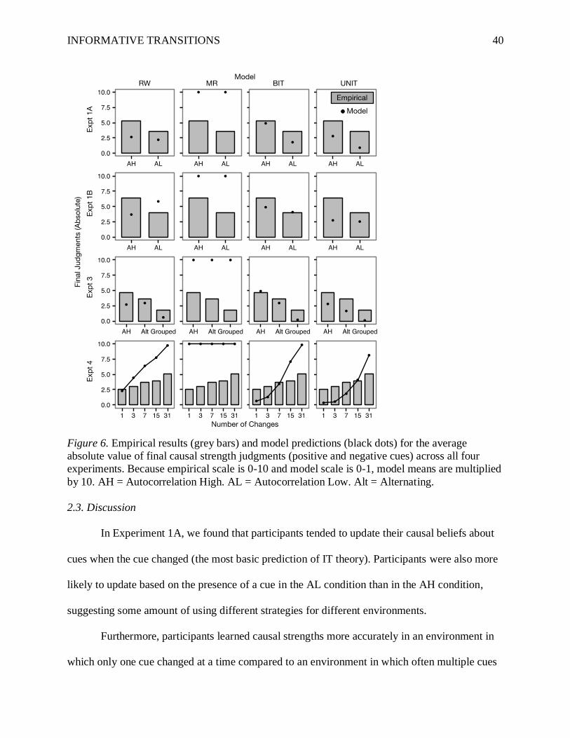
INFORMATIVE TRANSITIONS 40
Figure 6. Empirical results (grey bars) and model predictions (black dots) for the average
absolute value of final causal strength judgments (positive and negative cues) across all four
experiments. Because empirical scale is 0-10 and model scale is 0-1, model means are multiplied
by 10. AH = Autocorrelation High. AL = Autocorrelation Low. Alt = Alternating.
2.3. Discussion
In Experiment 1A, we found that participants tended to update their causal beliefs about
cues when the cue changed (the most basic prediction of IT theory). Participants were also more
likely to update based on the presence of a cue in the AL condition than in the AH condition,
suggesting some amount of using different strategies for different environments.
Furthermore, participants learned causal strengths more accurately in an environment in
which only one cue changed at a time compared to an environment in which often multiple cues
INFORMATIVE TRANSITIONS 41
changed at once. This provides some initial support for the hypothesis that people treat one-
change transitions as more informative.
One nuance, which will be examined more in Experiment 2, is that participants did
update their beliefs about cues when they changed, even when multiple other cues changed
simultaneously (the AL condition). Experiment 2 will provide a better test of whether
participants are more likely to update their beliefs after one-change vs. multi-change transitions.
With respect to the models, MR does a good job of capturing the trial-by-trial updating,
but not the final judgments. RW captures some of the final judgments, but not the trial-by-trial
updating when cues change. Both UNIT and BIT capture almost all of the trends, except that BIT
fails to capture the fact that subjects are more likely to update a cue when it is present than
absent, and both predict zero updating when a cue does not change (in reality there is some
updating when a cue does not change). Additionally, none of the models under consideration
captured the differences in accuracy in predicting the effect.
3. Experiment 1B: Learning with an Integer-Scale Effect
In Experiment 1B, we extended the paradigm from Experiment 1A, which used a binary
effect (e.g., Table 2), to an effect on the integer scale (e.g., Table 1). One advantage is simply to
extend the findings to a broader range of learning situations. A second advantage is that in
Experiment 1A we used a somewhat idiosyncratic way of creating the learning data that was
necessary to obtain the multiple regression features for the learning data. Using an integer scale
allows us to test a more straightforward data generation mechanism. We predicted the same
patterns of findings as in Experiment 1A.
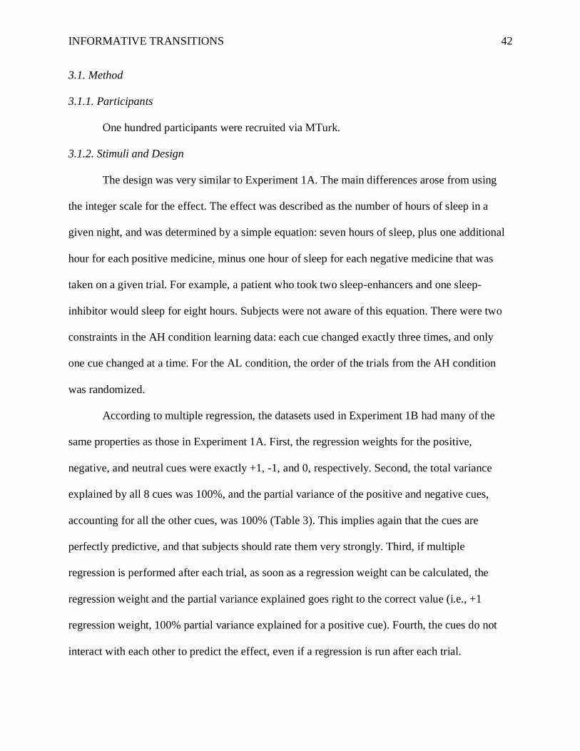
INFORMATIVE TRANSITIONS 42
3.1. Method
3.1.1. Participants
One hundred participants were recruited via MTurk.
3.1.2. Stimuli and Design
The design was very similar to Experiment 1A. The main differences arose from using
the integer scale for the effect. The effect was described as the number of hours of sleep in a
given night, and was determined by a simple equation: seven hours of sleep, plus one additional
hour for each positive medicine, minus one hour of sleep for each negative medicine that was
taken on a given trial. For example, a patient who took two sleep-enhancers and one sleep-
inhibitor would sleep for eight hours. Subjects were not aware of this equation. There were two
constraints in the AH condition learning data: each cue changed exactly three times, and only
one cue changed at a time. For the AL condition, the order of the trials from the AH condition
was randomized.
According to multiple regression, the datasets used in Experiment 1B had many of the
same properties as those in Experiment 1A. First, the regression weights for the positive,
negative, and neutral cues were exactly +1, -1, and 0, respectively. Second, the total variance
explained by all 8 cues was 100%, and the partial variance of the positive and negative cues,
accounting for all the other cues, was 100% (Table 3). This implies again that the cues are
perfectly predictive, and that subjects should rate them very strongly. Third, if multiple
regression is performed after each trial, as soon as a regression weight can be calculated, the
regression weight and the partial variance explained goes right to the correct value (i.e., +1
regression weight, 100% partial variance explained for a positive cue). Fourth, the cues do not
interact with each other to predict the effect, even if a regression is run after each trial.
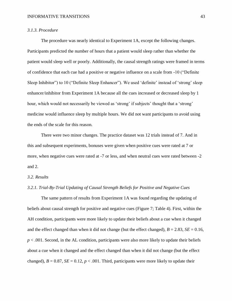
INFORMATIVE TRANSITIONS 43
3.1.3. Procedure
The procedure was nearly identical to Experiment 1A, except the following changes.
Participants predicted the number of hours that a patient would sleep rather than whether the
patient would sleep well or poorly. Additionally, the causal strength ratings were framed in terms
of confidence that each cue had a positive or negative influence on a scale from -10 (“Definite
Sleep Inhibitor”) to 10 (“Definite Sleep Enhancer”). We used ‘definite’ instead of ‘strong’ sleep
enhancer/inhibitor from Experiment 1A because all the cues increased or decreased sleep by 1
hour, which would not necessarily be viewed as ‘strong’ if subjects’ thought that a ‘strong’
medicine would influence sleep by multiple hours. We did not want participants to avoid using
the ends of the scale for this reason.
There were two minor changes. The practice dataset was 12 trials instead of 7. And in
this and subsequent experiments, bonuses were given when positive cues were rated at 7 or
more, when negative cues were rated at -7 or less, and when neutral cues were rated between -2
and 2.
3.2. Results
3.2.1. Trial-By-Trial Updating of Causal Strength Beliefs for Positive and Negative Cues
The same pattern of results from Experiment 1A was found regarding the updating of
beliefs about causal strength for positive and negative cues (Figure 7; Table 4). First, within the
AH condition, participants were more likely to update their beliefs about a cue when it changed
and the effect changed than when it did not change (but the effect changed), B = 2.83, SE = 0.16,
p < .001. Second, in the AL condition, participants were also more likely to update their beliefs
about a cue when it changed and the effect changed than when it did not change (but the effect
changed), B = 0.87, SE = 0.12, p < .001. Third, participants were more likely to update their
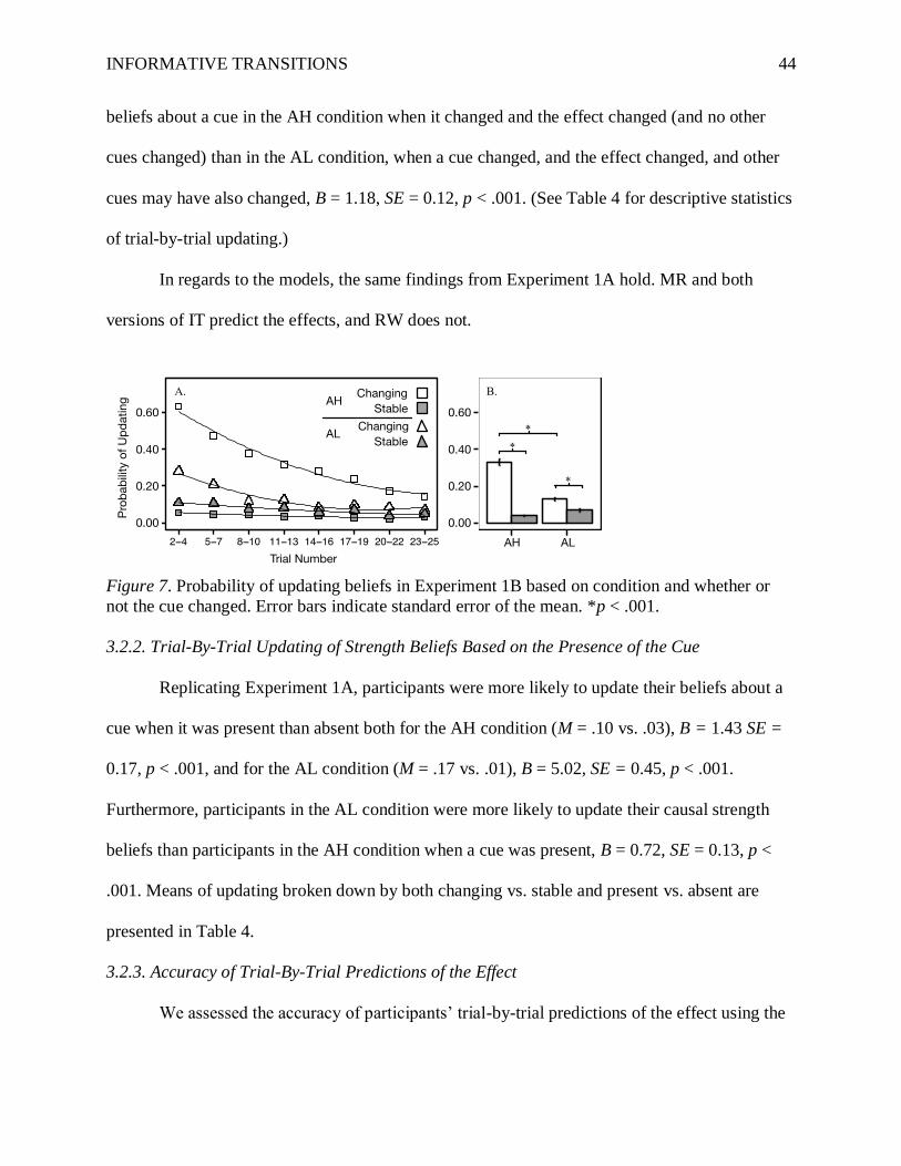
INFORMATIVE TRANSITIONS 44
beliefs about a cue in the AH condition when it changed and the effect changed (and no other
cues changed) than in the AL condition, when a cue changed, and the effect changed, and other
cues may have also changed, B = 1.18, SE = 0.12, p < .001. (See Table 4 for descriptive statistics
of trial-by-trial updating.)
In regards to the models, the same findings from Experiment 1A hold. MR and both
versions of IT predict the effects, and RW does not.
Figure 7. Probability of updating beliefs in Experiment 1B based on condition and whether or
not the cue changed. Error bars indicate standard error of the mean. *p < .001.
3.2.2. Trial-By-Trial Updating of Strength Beliefs Based on the Presence of the Cue
Replicating Experiment 1A, participants were more likely to update their beliefs about a
cue when it was present than absent both for the AH condition (M = .10 vs. .03), B = 1.43 SE =
0.17, p < .001, and for the AL condition (M = .17 vs. .01), B = 5.02, SE = 0.45, p < .001.
Furthermore, participants in the AL condition were more likely to update their causal strength
beliefs than participants in the AH condition when a cue was present, B = 0.72, SE = 0.13, p <
.001. Means of updating broken down by both changing vs. stable and present vs. absent are
presented in Table 4.
3.2.3. Accuracy of Trial-By-Trial Predictions of the Effect
We assessed the accuracy of participants’ trial-by-trial predictions of the effect using the
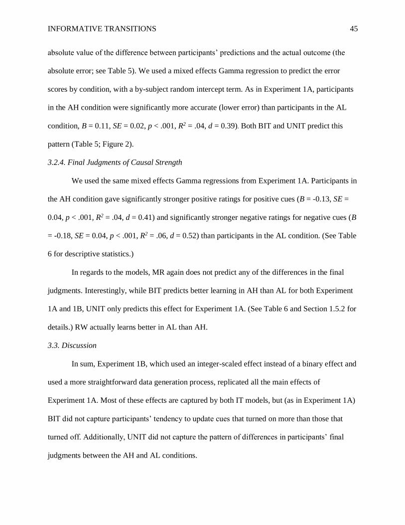
INFORMATIVE TRANSITIONS 45
absolute value of the difference between participants’ predictions and the actual outcome (the
absolute error; see Table 5). We used a mixed effects Gamma regression to predict the error
scores by condition, with a by-subject random intercept term. As in Experiment 1A, participants
in the AH condition were significantly more accurate (lower error) than participants in the AL
condition, B = 0.11, SE = 0.02, p < .001, R2 = .04, d = 0.39). Both BIT and UNIT predict this
pattern (Table 5; Figure 2).
3.2.4. Final Judgments of Causal Strength
We used the same mixed effects Gamma regressions from Experiment 1A. Participants in
the AH condition gave significantly stronger positive ratings for positive cues (B = -0.13, SE =
0.04, p < .001, R2 = .04, d = 0.41) and significantly stronger negative ratings for negative cues (B
= -0.18, SE = 0.04, p < .001, R2 = .06, d = 0.52) than participants in the AL condition. (See Table
6 for descriptive statistics.)
In regards to the models, MR again does not predict any of the differences in the final
judgments. Interestingly, while BIT predicts better learning in AH than AL for both Experiment
1A and 1B, UNIT only predicts this effect for Experiment 1A. (See Table 6 and Section 1.5.2 for
details.) RW actually learns better in AL than AH.
3.3. Discussion
In sum, Experiment 1B, which used an integer-scaled effect instead of a binary effect and
used a more straightforward data generation process, replicated all the main effects of
Experiment 1A. Most of these effects are captured by both IT models, but (as in Experiment 1A)
BIT did not capture participants’ tendency to update cues that turned on more than those that
turned off. Additionally, UNIT did not capture the pattern of differences in participants’ final
judgments between the AH and AL conditions.
INFORMATIVE TRANSITIONS 46
4. Experiment 2: Do Participants Learn More from One-Change Transitions?
In Experiments 1A and 1B, we found that learners were more likely to update their
beliefs about a positive cue when both the cue and the effect changed in the same direction,
compared to when the cue did not change but the effect changed. This finding corresponds to the
first main prediction of the Informative Transitions theory of causal learning, that changes in a
cue are some of the primary occasions of learning. We also found that that learners were more
likely to update their beliefs about a cue in the AH condition, when the cue changed by itself,
than in the AL condition. In the AL condition, when a cue changed, it sometimes changed by
itself, but often one or more than one of the other cues changed at the same time. This finding
provides initial support for the hypothesis that people are more likely to update their beliefs
during a one-change transition. According to IT theory, one-change transitions are more
informative because the other cues are held constant. However, one limitation of this comparison
is that in the AL condition, when a cue changed, sometimes it changed by itself, so the
manipulation between conditions was not as strong as it could be. The fact that we obtained
significant effects speaks to the strength of the phenomenon; however, it is still desirable to have
a cleaner comparison.
Experiment 2 was designed to carefully test whether participants selectively learn about a
cue when it is the only cue to change (a one-change transition) compared to when other cues
change as well. Instead of comparing two conditions, we used a within-subjects design, and
compared learning during transitions in which one, two, or three cues changed. We predicted that
participants would be more likely to update their beliefs about the influence of a cue when it
changed alone than when it changed at the same time as other cues.
INFORMATIVE TRANSITIONS 47
4.1. Method
4.1.1. Participants
One hundred participants were paid $3 for Experiment 2 and the subsequent experiments.
4.1.2. Design
One hundred and fifty datasets were created with 18 trials and 8 cues, and the effect was
an integer determined in the same way as in Experiment 1B. The data sets were designed so that
during each transition 0-3 cues changed, and most commonly 0-2 cues changed. This was
accomplished in the following way. On the first trial, we randomly determined the states of the
eight cues. During the next 17 trials, each cue changed at three randomly chosen times; see Table
7 for an example. Since they only changed three times, the cues were fairly autocorrelated; they
tended to remain in the same state for 6 trials in a row, on average. Because we wanted to have
the most power to detect differences between instances when only one cue changed vs. when two
cues changed, we only retained datasets in which the number of one-change and two-change
transitions were equivalent. This scheme meant that 0 cues changed in 24% of transitions, 1 or 2
cues changed in 29% of transitions each, and 3 cues changed in 18% of transitions. There were
no transitions in which 4 or more cues changed. The practice dataset was 12 trials in length and
was representative of the datasets participants would experience later in the procedure. Aside
from these changes, the design of the experiment was the same as Experiments 1A and 1B.
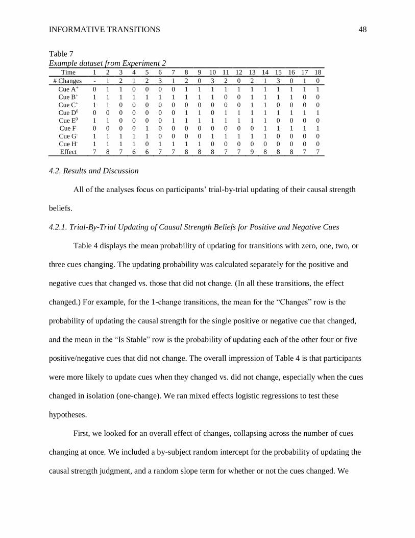
INFORMATIVE TRANSITIONS 48
Table 7
Example dataset from Experiment 2 Time 1 2 3 4 5 6 7 8 9 10 11 12 13 14 15 16 17 18
# Changes - 1 2 1 2 3 1 2 0 3 2 0 2 1 3 0 1 0
Cue A+ 0 1 1 0 0 0 0 1 1 1 1 1 1 1 1 1 1 1
Cue B+ 1 1 1 1 1 1 1 1 1 1 0 0 1 1 1 1 0 0
Cue C+ 1 1 0 0 0 0 0 0 0 0 0 0 1 1 0 0 0 0
Cue D0 0 0 0 0 0 0 0 1 1 0 1 1 1 1 1 1 1 1
Cue E0 1 1 0 0 0 0 1 1 1 1 1 1 1 1 0 0 0 0
Cue F- 0 0 0 0 1 0 0 0 0 0 0 0 0 1 1 1 1 1
Cue G- 1 1 1 1 1 0 0 0 0 1 1 1 1 1 0 0 0 0
Cue H- 1 1 1 1 0 1 1 1 1 0 0 0 0 0 0 0 0 0
Effect 7 8 7 6 6 7 7 8 8 8 7 7 9 8 8 8 7 7
4.2. Results and Discussion
All of the analyses focus on participants’ trial-by-trial updating of their causal strength
beliefs.
4.2.1. Trial-By-Trial Updating of Causal Strength Beliefs for Positive and Negative Cues
Table 4 displays the mean probability of updating for transitions with zero, one, two, or
three cues changing. The updating probability was calculated separately for the positive and
negative cues that changed vs. those that did not change. (In all these transitions, the effect
changed.) For example, for the 1-change transitions, the mean for the “Changes” row is the
probability of updating the causal strength for the single positive or negative cue that changed,
and the mean in the “Is Stable” row is the probability of updating each of the other four or five
positive/negative cues that did not change. The overall impression of Table 4 is that participants
were more likely to update cues when they changed vs. did not change, especially when the cues
changed in isolation (one-change). We ran mixed effects logistic regressions to test these
hypotheses.
First, we looked for an overall effect of changes, collapsing across the number of cues
changing at once. We included a by-subject random intercept for the probability of updating the
causal strength judgment, and a random slope term for whether or not the cues changed. We
INFORMATIVE TRANSITIONS 49
found that overall, participants were more likely to update their beliefs about a cue when it
changed and the effect changed than when it did not change (but the effect still changed), B =
1.94, SE = 0.11, p < .001. Next, we examined this same effect when one, two, or three cues
changed, using the same random effects terms. Participants were more likely to update their
beliefs about cues when they changed than when they were stable within transitions in which one
cue changed (B = 2.49, SE = 0.17, p < .001), two cues changed (B = 2.00, SE = 0.14, p < .001),
and three cues changed (B = 1.66, SE = 0.18, p < .001).
Finally, and most importantly, we compared the probability of belief updating when cues
changed in transitions in which one, two, or three cues changed. Again, we only examined
transitions in which the effect also changed. We included a by-subject random intercept for the
probability of updating the causal strength judgment, and a random slope term for the number of
cues that changed. Participants were more likely to update their beliefs about the single cue that
changed in a one-change transition than for the two cues that changed in a two-change transition
(B = 0.43, SE = 0.10, p < .001), and in a two-change transition compared to a three-change
transition (B = 0.29, SE = 0.11, p < .01). (See Figure 8 and Table 4.)
With respect to the models, as in the prior experiments, RW does not predict the effect,
but MR, BIT, and UNIT predict the general pattern. The reason that MR predicts this effect has
to do with the fact that a cue must not be confounded with another cue (two-change and three-
change transitions) for learning to occur.
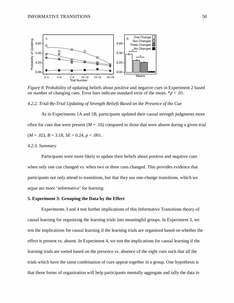
INFORMATIVE TRANSITIONS 50
Figure 8. Probability of updating beliefs about positive and negative cues in Experiment 2 based
on number of changing cues. Error bars indicate standard error of the mean. *p < .01.
4.2.2. Trial-By-Trial Updating of Strength Beliefs Based on the Presence of the Cue
As in Experiments 1A and 1B, participants updated their causal strength judgments more
often for cues that were present (M = .16) compared to those that were absent during a given trial
(M = .02), B = 3.18, SE = 0.24, p < .001.
4.2.3. Summary
Participants were more likely to update their beliefs about positive and negative cues
when only one cue changed vs. when two or three cues changed. This provides evidence that
participants not only attend to transitions, but that they use one-change transitions, which we
argue are more ‘informative’ for learning.
5. Experiment 3: Grouping the Data by the Effect
Experiments 3 and 4 test further implications of this Informative Transitions theory of
causal learning for organizing the learning trials into meaningful groups. In Experiment 3, we
test the implications for causal learning if the learning trials are organized based on whether the
effect is present vs. absent. In Experiment 4, we test the implications for causal learning if the
learning trials are sorted based on the presence vs. absence of the eight cues such that all the
trials which have the same combination of cues appear together in a group. One hypothesis is
that these forms of organization will help participants mentally aggregate and tally the data in
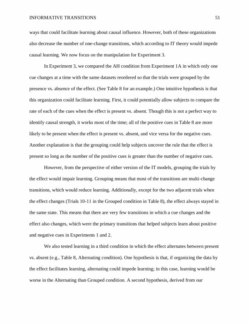
INFORMATIVE TRANSITIONS 51
ways that could facilitate learning about causal influence. However, both of these organizations
also decrease the number of one-change transitions, which according to IT theory would impede
causal learning. We now focus on the manipulation for Experiment 3.
In Experiment 3, we compared the AH condition from Experiment 1A in which only one
cue changes at a time with the same datasets reordered so that the trials were grouped by the
presence vs. absence of the effect. (See Table 8 for an example.) One intuitive hypothesis is that
this organization could facilitate learning. First, it could potentially allow subjects to compare the
rate of each of the cues when the effect is present vs. absent. Though this is not a perfect way to
identify causal strength, it works most of the time; all of the positive cues in Table 8 are more
likely to be present when the effect is present vs. absent, and vice versa for the negative cues.
Another explanation is that the grouping could help subjects uncover the rule that the effect is
present so long as the number of the positive cues is greater than the number of negative cues.
However, from the perspective of either version of the IT models, grouping the trials by
the effect would impair learning. Grouping means that most of the transitions are multi-change
transitions, which would reduce learning. Additionally, except for the two adjacent trials when
the effect changes (Trials 10-11 in the Grouped condition in Table 8), the effect always stayed in
the same state. This means that there are very few transitions in which a cue changes and the
effect also changes, which were the primary transitions that helped subjects learn about positive
and negative cues in Experiments 1 and 2.
We also tested learning in a third condition in which the effect alternates between present
vs. absent (e.g., Table 8, Alternating condition). One hypothesis is that, if organizing the data by
the effect facilitates learning, alternating could impede learning; in this case, learning would be
worse in the Alternating than Grouped condition. A second hypothesis, derived from our
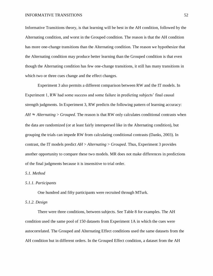
INFORMATIVE TRANSITIONS 52
Informative Transitions theory, is that learning will be best in the AH condition, followed by the
Alternating condition, and worst in the Grouped condition. The reason is that the AH condition
has more one-change transitions than the Alternating condition. The reason we hypothesize that
the Alternating condition may produce better learning than the Grouped condition is that even
though the Alternating condition has few one-change transitions, it still has many transitions in
which two or three cues change and the effect changes.
Experiment 3 also permits a different comparison between RW and the IT models. In
Experiment 1, RW had some success and some failure in predicting subjects’ final causal
strength judgments. In Experiment 3, RW predicts the following pattern of learning accuracy:
AH ≈ Alternating > Grouped. The reason is that RW only calculates conditional contrasts when
the data are randomized (or at least fairly interspersed like in the Alternating condition), but
grouping the trials can impede RW from calculating conditional contrasts (Danks, 2003). In
contrast, the IT models predict AH > Alternating > Grouped. Thus, Experiment 3 provides
another opportunity to compare these two models. MR does not make differences in predictions
of the final judgments because it is insensitive to trial order.
5.1. Method
5.1.1. Participants
One hundred and fifty participants were recruited through MTurk.
5.1.2. Design
There were three conditions, between subjects. See Table 8 for examples. The AH
condition used the same pool of 150 datasets from Experiment 1A in which the cues were
autocorrelated. The Grouped and Alternating Effect conditions used the same datasets from the
AH condition but in different orders. In the Grouped Effect condition, a dataset from the AH
INFORMATIVE TRANSITIONS 53
condition was split into effect-present and effect-absent groups. The trials within each group
were randomly ordered, and either the effect-present or effect-absent group was randomly
presented first. On average, 3.26 (SD=1.80) cues changed per transition.
For the Alternating Effect condition, we used a computer program to randomly rearrange
the order of the trials from the AH condition datasets in a way that maximized the number of
alternations between effect-present and effect-absent trials. Because the numbers of effect-
present and effect-absent trials were often not equal, sometimes the effect stayed the same for
two or three trials (e.g., Trials 3-4 in the Alternating condition in Table 8). On average, 3.29
(SD=1.77) cues changed per transition.
Each participant was randomly assigned to one of the three conditions, and viewed one
randomly selected dataset of each type (two positive, two negative, or two neutral cues; see
Section 2.1.2.1.). The order in which the three datasets were presented was also randomized.
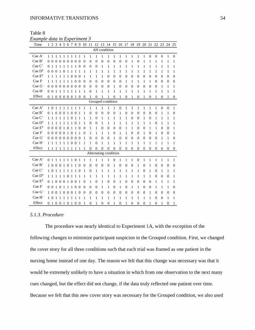
INFORMATIVE TRANSITIONS 54
Table 8
Example data in Experiment 3 Time 1 2 3 4 5 6 7 8 9 10 11 12 13 14 15 16 17 18 19 20 21 22 23 24 25
AH condition
Cue A+ 1 1 1 1 1 1 1 1 1 1 1 1 1 1 1 1 1 1 1 1 0 0 0 1 0
Cue B+ 0 0 0 0 0 0 0 0 0 0 0 0 0 0 0 0 0 1 0 1 1 1 1 1 1
Cue C+ 0 1 1 1 1 1 1 1 0 0 0 0 1 1 1 1 1 1 1 1 1 1 1 1 1
Cue D0 0 0 0 1 0 1 1 1 1 1 1 1 1 1 1 1 1 1 1 1 1 1 1 1 1
Cue E0 1 1 1 1 1 1 0 0 0 1 1 1 1 0 0 0 0 0 0 0 0 0 0 0 0
Cue F- 1 1 1 1 1 1 1 0 0 0 0 0 0 0 0 0 1 1 1 1 1 0 0 0 0
Cue G- 0 0 0 0 0 0 0 0 0 0 0 0 0 0 1 0 0 0 0 0 0 0 1 1 1
Cue H- 0 0 1 1 1 1 1 1 1 1 0 1 1 1 1 1 1 1 1 1 1 1 1 1 1
Effect 0 1 0 0 0 0 0 1 0 0 1 0 1 1 0 1 0 1 0 1 0 1 0 1 0
Grouped condition
Cue A+ 1 0 1 1 1 1 1 1 1 1 1 1 1 1 1 0 1 1 1 1 1 1 0 0 1
Cue B+ 0 1 0 0 0 1 0 0 1 1 0 0 0 0 0 1 0 0 0 0 0 0 1 1 0
Cue C+ 1 1 1 1 1 1 0 1 1 1 1 0 1 1 1 1 1 0 0 1 0 1 1 1 1
Cue D0 1 1 1 1 1 1 1 0 1 1 0 0 1 1 1 1 1 1 1 1 1 0 1 1 1
Cue E0 0 0 0 0 1 0 1 1 0 0 1 1 0 0 0 0 1 1 0 0 1 1 0 0 1
Cue F- 0 0 0 0 0 1 0 1 1 0 1 1 1 1 0 1 1 0 0 1 0 1 0 0 1
Cue G- 0 0 0 0 0 0 0 0 0 1 0 0 0 0 1 0 0 0 0 0 0 0 1 1 0
Cue H- 1 1 1 1 1 1 0 0 1 1 1 0 1 1 1 1 1 1 1 1 1 1 1 1 1
Effect 1 1 1 1 1 1 1 1 1 1 0 0 0 0 0 0 0 0 0 0 0 0 0 0 0
Alternating condition
Cue A+ 0 1 1 1 1 1 1 0 1 1 1 1 1 1 0 1 1 1 0 1 1 1 1 1 1
Cue B+ 1 0 0 0 1 0 1 1 0 0 0 0 0 0 1 0 0 0 1 0 1 0 0 0 0
Cue C+ 1 0 1 1 1 1 1 1 0 1 0 1 1 1 1 1 1 1 1 0 1 0 1 1 1
Cue D0 1 1 1 1 1 0 1 1 1 1 1 1 1 1 1 1 1 1 1 1 1 0 0 0 1
Cue E0 0 1 0 0 0 1 0 0 1 0 1 0 1 0 0 1 0 0 0 0 0 1 1 1 1
Cue F- 0 0 1 0 1 1 1 0 0 0 0 0 1 1 0 1 0 1 1 0 0 1 1 1 0
Cue G- 1 0 0 1 0 0 0 1 0 0 0 0 0 0 0 0 0 0 0 0 1 0 0 0 0
Cue H- 1 0 1 1 1 1 1 1 1 1 1 1 1 1 1 1 1 1 1 1 1 0 0 1 1
Effect 0 1 0 0 1 0 1 0 0 1 0 1 0 0 1 0 1 0 0 0 1 0 1 0 1
5.1.3. Procedure
The procedure was nearly identical to Experiment 1A, with the exception of the
following changes to minimize participant suspicion in the Grouped condition. First, we changed
the cover story for all three conditions such that each trial was framed as one patient in the
nursing home instead of one day. The reason we felt that this change was necessary was that it
would be extremely unlikely to have a situation in which from one observation to the next many
cues changed, but the effect did not change, if the data truly reflected one patient over time.
Because we felt that this new cover story was necessary for the Grouped condition, we also used
INFORMATIVE TRANSITIONS 55
it for the other two conditions to hold it constant. In addition, participants in the Grouped
condition were told that the data would be presented in an order such that they would first see
either all of the patients who slept well or all of the patients who slept poorly; we felt that an
explanation was needed because the organization was so obvious. Participants in the other two
conditions were not told how the data were organized. The three datasets were framed as three
nursing homes, with 25 patients (trials) each. Finally, the practice dataset consisted of 9 trials,
and the practice dataset was ordered according to experimental condition.
5.2. Results and Discussion
5.2.1. Final Judgments of Positive and Negative Cues
The analysis focused on participants’ final judgments of causal strength (Table 6).5 We
performed a mixed effects Gamma regression with a random intercept for each participant and
fixed effects for condition (between Ss), just as in Experiment 1A. For positive cues, participants
in the AH condition gave the strongest causal strength judgments, followed by the Alternating
condition, and lastly the Grouped condition. The difference between AH vs. Alternating was
marginal (B = -0.03, SE = 0.02, p = .08, R2 = .01, d = 0.15), and the difference between
Alternating and Grouped was significant (B = -0.02, SE = 0.01, p = .03, R2 = .01, d = 0.18). The
difference between AH vs. Grouped was significant (B = -0.06, SE = 0.02, p < .001, R2 = .03, d
= 0.34). For negative cues, judgments from participants in the AH condition were marginally
stronger than those in the Alternating condition (B = -0.03, SE = 0.02, p = .05, R2 = .01, d =
0.15), and the difference between Alternating and Grouped was significant (B = -0.03, SE = 0.01,
p < .001, R2 = .02, d = 0.30). The difference between AH and Grouped was significant (B = -
5The trial-by-trial data were accidentally not recorded for this experiment. However, this is not a
critical problem because the primary hypotheses for this experiment were about the final
judgments; it is less interesting to examine trial-by-trial changes in the Grouped condition
because the transitions-based theory predicts few updates.
INFORMATIVE TRANSITIONS 56
0.07, SE = 0.02, p < .001, R2 = .05, d = 0.46).
With regard to the models, RW captures the distinction between the Grouped condition
vs. the other two conditions, but not between the AH vs. Alternating conditions. BIT and UNIT
predict differences between all three conditions. For both the positive and negative cues, the
difference between the AH and Alternating conditions were borderline significant.
5.2.2. Summary and Discussion
The pattern of results for the positive and negative cues corresponds with the predictions
made by the IT models and RW. Participants performed worst in the Grouped condition in which
the cues often changed but the effect rarely changed; organizing the learning data apparently
does not facilitate causal learning. They performed marginally better in the AH condition with
many one-change transitions than the Alternating condition with many transitions in which
multiple cues changed and the effect often changed, which was predicted by the IT models but
not RW.
6. Experiment 4: Sorting the Data by the Cues
In Experiment 3, we found that participants had difficulty learning causal strength when
the trials were sorted by the state of the effect. In Experiment 4, we tested the implication of
organizing the trials by the states of the cues. We sorted the trials based on the eight cues (e.g.,
Table 9), similar to how the rows are organized in a truth table, to make the data as organized as
possible for the learner.
In this sorting system, some cues change only a few times, whereas others change very
frequently. According to our transitions-based theory of causal learning, it should be easier to
learn about the cues that change more frequently for two reasons. First, the cue that changes most
frequently (e.g., Cue H in Table 9) is the only one that has any one-change transitions. Second,
INFORMATIVE TRANSITIONS 57
both versions of the IT models predict that people learn more even in a multi-change transition
than if the cue does not change. For this reason, we expected learning to be better for the cues
that changed more frequently (Cues E-H in Table 9) than the cues that changed less frequently
(Cues A-D in Table 9).
If these predictions hold, it would slightly change the interpretation of the IT theory. In
Experiments 1A and 1B, data with high as opposed to low autocorrelation produced better
learning. The IT predictions for Experiment 4 are that people will learn better about the cues that
change more frequently, which have low (in fact negative) autocorrelation, relative to the cues
with high autocorrelation. The logic of this hypothesis is that in general learning is better in a
highly autocorrelated environment, but for an individual cue it helps for the cue to have low or
negative autocorrelation (within a highly autocorrelated environment).
6.1. Method
6.1.1. Participants
One hundred participants were recruited via MTurk.
6.1.2. Design and Procedure
We created a new pool of 150 datasets with 32 trials. The effect was an integer
determined in the same way as in Experiment 1B. The length of 32 trials was chosen because it
is a power of two, which allowed the datasets to have 5 cues that changed every 1 (Cue H), 2
(Cue G), 4 (Cue F), 8 (Cue E), or 16 (Cue D) trials. This means that the datasets had cues that
changed 1, 3, 7, 15, or 31 times (Cue D-H). We wanted to use eight cues, like in the previous
experiments, instead of just five, so we added three additional cues (A-C) that changed once
between trials 8 and 24, randomly chosen.
The cover story involved a single patient observed repeatedly over time like in
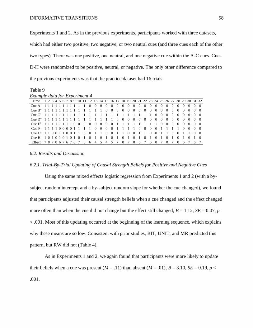
INFORMATIVE TRANSITIONS 58
Experiments 1 and 2. As in the previous experiments, participants worked with three datasets,
which had either two positive, two negative, or two neutral cues (and three cues each of the other
two types). There was one positive, one neutral, and one negative cue within the A-C cues. Cues
D-H were randomized to be positive, neutral, or negative. The only other difference compared to
the previous experiments was that the practice dataset had 16 trials.
Table 9
Example data for Experiment 4 Time 1 2 3 4 5 6 7 8 9 10 11 12 13 14 15 16 17 18 19 20 21 22 23 24 25 26 27 28 29 30 31 32
Cue A+ 1 1 1 1 1 1 1 1 1 1 1 0 0 0 0 0 0 0 0 0 0 0 0 0 0 0 0 0 0 0 0 0
Cue B+ 1 1 1 1 1 1 1 1 1 1 1 1 1 1 0 0 0 0 0 0 0 0 0 0 0 0 0 0 0 0 0 0
Cue C+ 1 1 1 1 1 1 1 1 1 1 1 1 1 1 1 1 1 1 1 1 1 1 1 0 0 0 0 0 0 0 0 0
Cue D0 1 1 1 1 1 1 1 1 1 1 1 1 1 1 1 1 0 0 0 0 0 0 0 0 0 0 0 0 0 0 0 0
Cue E0 1 1 1 1 1 1 1 1 0 0 0 0 0 0 0 0 1 1 1 1 1 1 1 1 0 0 0 0 0 0 0 0
Cue F- 1 1 1 1 0 0 0 0 1 1 1 1 0 0 0 0 1 1 1 1 0 0 0 0 1 1 1 1 0 0 0 0
Cue G- 1 1 0 0 1 1 0 0 1 1 0 0 1 1 0 0 1 1 0 0 1 1 0 0 1 1 0 0 1 1 0 0
Cue H- 1 0 1 0 1 0 1 0 1 0 1 0 1 0 1 0 1 0 1 0 1 0 1 0 1 0 1 0 1 0 1 0
Effect 7 8 7 8 6 7 6 7 6 7 6 6 4 5 4 5 7 8 7 8 6 7 6 8 7 8 7 8 6 7 6 7
6.2. Results and Discussion
6.2.1. Trial-By-Trial Updating of Causal Strength Beliefs for Positive and Negative Cues
Using the same mixed effects logistic regression from Experiments 1 and 2 (with a by-
subject random intercept and a by-subject random slope for whether the cue changed), we found
that participants adjusted their causal strength beliefs when a cue changed and the effect changed
more often than when the cue did not change but the effect still changed, B = 1.12, SE = 0.07, p
< .001. Most of this updating occurred at the beginning of the learning sequence, which explains
why these means are so low. Consistent with prior studies, BIT, UNIT, and MR predicted this
pattern, but RW did not (Table 4).
As in Experiments 1 and 2, we again found that participants were more likely to update
their beliefs when a cue was present (M = .11) than absent (M = .01), B = 3.10, SE = 0.19, p <
.001.
INFORMATIVE TRANSITIONS 59
6.2.2. Final Judgments of Causal Strength
Because we did not expect the number of changes to map proportionally onto causal
strength judgments, we recoded the cues that changed 1, 3, 7, 15, or 31 times as 1, 2, 3, 4, and 5,
respectively. We then entered this predictor into a mixed effects Gamma regression with a by-
subject random intercept and a by-subjects random slope for the number of times that the cue
changed. Participants made stronger final causal strength judgments for cues that changed more,
both for positive (B = -0.15, SE = 0.03, p < .001, R2 = .02, d = 0.27) and negative cues (B = -
0.12, SE = 0.03, p < .001, R2 = .02, d = 0.29). (See Table 6 for descriptive statistics.)
6.2.3. Discussion
Experiment 4 revealed, similarly to Experiment 3, that ‘organizing’ the data into blocks
does not inherently help the learner. Participants learned the best about cues that frequently
changed state, and learned the worst about cues that were highly stable. Another way to think
about this finding is that even though learning is better in a highly autocorrelated environment
than in an environment with low autocorrelation (Experiments 1A and 1B), for an individual cue
in a highly autocorrelated environment, it helps for the cue to change frequently (low
autocorrelation).
7. General Discussion
In four experiments, we tested how people learn which of multiple possible cues have
positive, negative, or no influence on an effect. The key novel finding is that participants tend to
learn about and update their beliefs about the strength of an individual cue when it changes. This
is especially true when a cue turns on (rather than off), and also when a cue changes by itself and
all the other cues do not change. Because of this feature of learning, participants’ final causal
strength judgments are more accurate in environments in which the cues tend to remain fairly
INFORMATIVE TRANSITIONS 60
stable over time, and usually only one cue changes at a time. These findings hold for a variety of
important environments including positively autocorrelated environments, randomized
environments, and environments in which the experiences are 'organized' or sorted based on the
states of the cues or effect. Though in the paper we focused on positive and negative cues, in the
Appendix we report similar findings for neutral cues. Table 10 (see also Figures 4 and 6)
documents the key findings, other related findings, and the predictions of all the models.
To account for these results, we developed two ‘Informative Transitions’ models, in
which learning is informed by cue/effect transitions between timepoints. Overall, our IT models
captured most of the findings. At the same time, Table 10 (also Figures 4 and 6) makes clear that
neither of the IT models are perfect. (The same can be said of our findings regarding neutral
cues; see Appendix A and Table A2.) In particular, the IT models predict no updating when cues
do not change; in reality there is some degree of updating. Furthermore, there is considerably
more updating when cues are stable and present, rather than absent, especially in the
Autocorrelation Low condition. This effect is uniquely predicted by RW. Lastly, none of the
models predict the different patterns of updating in the AH vs. AL conditions, though the two IT
models do a good job of predicting differences between conditions in the final judgments.
Overall, these findings uncover a number of new features of human learning, and though the
models do help to explain them, there is clearly more work to be done to accurately capture all
these findings.
Our view on the adaptive rationality of IT can be summarized in the following way. 1)
Focusing on changes is normative in time series environments. 2) Focusing on changes is not
justified in non-time series environments, but 3) it is consistent with the tendency to see positive
autocorrelation even when learning data have zero autocorrelation, and 4) it costs very little in

INFORMATIVE TRANSITIONS 61
terms of learning efficiency and accuracy. 5) In light of these considerations, parsimony
demands consideration of the possibility that learners focus on changes in all environments.
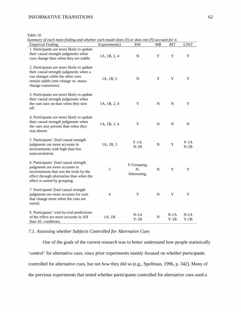
INFORMATIVE TRANSITIONS 62
Table 10
Summary of each main finding and whether each model does (Y) or does not (N) account for it.
Empirical Finding Experiment(s) RW MR BIT UNIT
1. Participants are more likely to update
their causal strength judgments when
cues change than when they are stable.
1A, 1B, 2, 4 N Y Y Y
2. Participants are more likely to update
their causal strength judgments when a
cue changes while the other cues
remain stable (one-change vs. many-
change transitions).
1A, 1B, 2 N Y Y Y
3. Participants are more likely to update
their causal strength judgments when
the cues turn on than when they turn
off.
1A, 1B, 2, 4 Y N N Y
4. Participants are more likely to update
their causal strength judgments when
the cues stay present than when they
stay absent.
1A, 1B, 2, 4 Y N N N
5. Participants’ final causal strength
judgments are more accurate in
environments with high than low
autocorrelation.
1A, 1B, 3 Y-1A.
N-1B N Y
Y-1A
N-1B
6. Participants’ final causal strength
judgments are more accurate in
environments that sort the trials by the
effect through alternation than when the
effect is sorted by grouping.
3
Y-Grouping.
N-
Alternating.
N Y Y
7. Participants' final causal strength
judgments are more accurate for cues
that change more when the cues are
sorted.
4 Y N Y Y
8. Participants’ trial-by-trial predictions
of the effect are more accurate in AH
than AL conditions.
1A, 1B N-1A
Y-1B N
N-1A
Y-1B
N-1A
Y-1B
7.1. Assessing whether Subjects Controlled for Alternative Cues
One of the goals of the current research was to better understand how people statistically
‘control’ for alternative cues, since prior experiments mainly focused on whether participants
controlled for alternative cues, but not how they did so (e.g., Spellman, 1996, p. 342). Many of
the previous experiments that tested whether participants controlled for alternative cues used a
INFORMATIVE TRANSITIONS 63
design involving Simpson’s paradox with two cues (e.g., Spellman, 1996; Spellman et al., 2001,
Waldmann & Hagmayer, 2001). However, we could not use this paradigm in the current
experiements: the design was developed for two cues, and even if we could figure out a way to
generalize the Simpson’s paradox design to eight cues, it still would not allow us to test the
hypotheses about one-change transitions. Still, our design does permit us to infer whether
participants controlled for alternative cues using a different logic.
In the current experiments, the partial variance explained by the positive and negative
cues (controlling for all the other cues) is 100%. In contrast, the variance explained by a single
cue in a bivariate analysis was sometimes as low as 7% (Table 3). Because we do not expect
variance explained to map linearly onto our causal strength scale, we cannot interpret the
absolute value of a causal strength judgment; we cannot say whether an average causal strength
rating of roughly 5 (Experiment 1A) or 6 (Experiment 1B) on a -10 to +10 scale means that
participants did or did not control for alternative cues. However, all the manipulations that
caused participants to give more extreme causal strength ratings (e.g., AH vs. AL conditions in
Experiments 1A and 1B, AH vs. Alternating Effect vs. Grouped Effect in Experiment 3, and
sorting in Experiment 4) can be viewed as helping participants to control for alternative cues and
thereby infer stronger, more accurate causal strengths.
7.2. Focal Sets
There is another prominent theory of how people control for alternative cues, which has
not yet been addressed in this paper, called Focal Set theory (Cheng & Novick, 1990; Cheng &
Holyoak, 1995; Cheng, 1997). According to this theory, when assessing the strength of a target
cue on an effect, learners focus on a subset of the data in which the other factor(s) are constant.
Then, within this focal set, the learner could compute causal influence by using measures of
INFORMATIVE TRANSITIONS 64
causal strength for situations involving a single cue and effect such as ∆P (Jenkins & Ward,
1965) or Power PC (Cheng, 1997), or any one of a number of other options (e.g., Hattori &
Oaksford, 2007). Though focal set theory is intuitively appealing because of its simplicity, there
are several theoretical problems with the theory that have been left unresolved, so that in many
situations, especially when there are more than just a few cues, the theory either fails to make a
single prediction (e.g., Kim, Markman, & Kim, 2016) or cannot make any predictions at all.
The first problem is that it is unclear exactly how people would use focal sets to control
for multiple alternative cues. One issue is that as the number of cues increases, the number of
possible focal sets increases exponentially. Specifically, there are 2n focal sets for n alternative
binary cues. For example, if there are three alternative cues, one could choose the focal set in
which all three are absent, or the first two are present but the third is absent, etc. In this way, a
learner may be forced to choose arbitrarily between multiple possible focal sets. Another
problem is that when there are many alternative cues, but a limited number of learning trials,
there might be no usable focal sets. For a focal set to be usable within a particular set of learning
data, the data must include at least one trial in which the target cue is present and another in
which the target cue is absent within the given focal set. Going back to the example when there
are three alternative cues, there may not be any trials in which all three alternative cues are
absent. Even if there is at least one trial in which all three alternative cues are absent, there may
not be a pair of trials for which the target cue is present and absent, while the alternatives are all
absent. Most previous research has focused on scenarios in which there are only two cues, in
which case these issues do not arise.
The second problem is that searching for usable focal sets would be computationally
challenging and require unrealistically large memory resources. There are often very few usable
INFORMATIVE TRANSITIONS 65
focal sets, which means that a learner must keep track of all the data; the learner cannot start the
learning scenario only storing data from a certain pre-specified focal set and forgetting the other
trials. To demonstrate this, we conducted a simulation of 1000 datasets, each with eight binary
cues and 25 trials. For each trial, each cue had a 50% chance of being 1 or 0. For a given cue,
there were 0 usable focal sets 30% of the time, 1 usable focal set 40% of the time, 2 usable focal
sets 22% of the time, and 3 or more usable focal sets 8% of the time. Further, the vast majority of
the usable focal sets contained only two trials. Because there will be a small number of usable
focal sets out of the 27=128 possible focal sets for a given target cue, the learner cannot enter the
scenario focusing only on one particular focal set and ignoring all the trials that do not fit that
focal set. This means that the learner would have to search for usable focal sets retrospectively,
which would be overwhelming. Because of these challenges, the details of how the focal set
theory would actually be implemented in the context of many alternative cues have been left
unspecified, and we do not consider it as a viable option for learning in the current experiments.
However, in a sense, one-change transitions can be viewed as a local focal set; all the
other cues are held constant while the state of the target cue varies. In the Informative
Transitions theory, a learner can dynamically use many different focal sets over time. For
example, in the AH condition in Table 1, when estimating the influence of Cue A, the learner
could use one focal set for Trials 3-4, a second for Trials 6-7, and a third for Trials 9-10. Another
way in which the Informative Transitions theory differs from focal sets is that according to the
Informative Transitions theory, learning will be very difficult in the AL condition in Table 1
because there are no adjacent trials which comprise one-change transitions for Cue A. In
contrast, focal set theory is insensitive to the order, so in theory a learner could use the focal sets
inherent in Trial Numbers 3 vs. 4, 6 vs. 7, or 9 vs. 10 even though they are not adjacent in the AL
INFORMATIVE TRANSITIONS 66
condition.
7.3. Grouping of Trials in Causality Research and Categorization
There are two sets of findings from the prior literature that are especially relevant to the
grouping manipulations used in the current experiments.
7.3.1. Categorization Research on Grouping
Experiment 3, which compared Grouped Effect vs. Alternating Effect conditions, is
similar to a number of studies of category learning that have compared performance after the
learning exemplars of different categories were either blocked or interleaved. The more effective
strategy seems to depend on the structure of the task. Noh, Yan, Bjork, and Maddox (2016)
argued that blocking helps for rule-based categories, in which verbalizable rules can reliably
predict the category given the cues, whereas alternation helps for information-integration
categories, in which the relation between the cues and the category is not easily verbalizable.
If we conceptualize our stimuli as falling into categories of “effect present” or “effect
absent” in Experiments 1A and 3, our stimuli are arguably rule-based categories in that simple,
verbalizable linear rules can be used to predict the effect perfectly given the cues. (For example,
in Table 2, the effect equals 1 plus 1 for each positive cue that is present minus 1 for each
negative cue that is present.) However, unlike what was found for categorization, that blocking
facilitates learning rule-based categories, in Experiment 3 we found that alternating facilitated
learning.
One possible explanation why our results seem to contradict Noh et al.’s (2016) findings
is that blocking is superior when the task involves discriminating between fairly easily
discriminable categories (Carvalho & Goldstone, 2014; Zulkiply & Burt, 2013). Arguably our
stimuli in Experiments 1A and 3 form high-similarity categories that are difficult to discriminate;
INFORMATIVE TRANSITIONS 67
the difference between a trial in which the effect is present and one in which it is absent may
depend upon the difference of just one cue, and none of the cues are necessary or sufficient.
More generally, if this categorization work applies to causal learning, it will be important to
more thoroughly investigate the circumstances under which one-change transitions and
interleaving effects are helpful.
7.3.2. Causal Learning Research on Grouping
Our Experiment 4, which organized the trials by sorting them based on the eight cues, is
somewhat similar to a manipulation used in Waldmann and Hagmayer’s (2001) Experiment 2. In
their study, there was a target cue and an alternative cue, and one binary effect. The learning
trials were presented either in a random order or organized into blocks based on the alternative
cue. Participants in the blocked condition were more likely to adequately control for the alternate
cue than in the randomized condition. (In our terminology, the blocked condition had many one-
change transitions for the target cue.)
In our Experiment 4, we found that learning was better for cues that frequently changed
than those that rarely changed (were organized into blocks). One interpretation of this finding, in
line with Waldmann and Hagmayer’s (2001) study, is that organizing some cues into blocks
facilitated learning about the other cues that changed more frequently. Experiments 1A and 1B
can be viewed under a similar interpretation; in the AH conditions, the cues are fairly stable
(grouped into blocks), which collectively facilitated learning about all eight cues.
In sum, one-change transitions and ‘grouping’ can be viewed as opposite sides of the
same phenomenon; one-change transitions arise to the extent that alternative cues are stable
(grouped). The current experiments demonstrate the wide-ranging implications for grouping, and
identify one-change transitions as the occasions of learning.
INFORMATIVE TRANSITIONS 68
7.4 Connections with other Theories of Learning
A number of theories of causal learning are relevant to learning about multiple cues
simultaneously. Lu, Yuille, Liljeholm, Cheng, and Holyoak (2008; see also Powell, Merrick, Lu,
& Holyoak, 2016) proposed that people approach learning about a set of potentially relevant cues
with priors that only a small number are actually causes, and those that are causes are very
strong. Yeung and Griffiths (2015) also suggest that people initially believe that causes are likely
to be deterministic. Griffiths and Tenenbaum (2005) proposed that when people infer causal
strength, that they are really trying to calculate whether a cue is a cause or not. Though all of
these studies only involved one to three cues, perhaps one way to think about these findings is
that subjects’ priors and goals could direct their attention when learning about multiple causes;
they might try to initially learn about a limited number of very strong cues, and then only later
begin to entertain the possibility that there are multiple causes, and to learn the relative strengths
of all of the causes. It could be useful in future work to generalize these theories to larger
numbers of causes.
In another front, even though many causal learning theories (e.g., citations in prior
paragraph) focus mainly on final causal strengths at the end of learning, research on
reinforcement learning has a much stronger emphasis on what is being learned trial-by-trial as
well as the neural correlates of learning. Furthermore, many reinforcement learning tasks are
similar to the current studies in that they involve learning about multiple probabilistic cues (e.g.,
Foerde, Knowlton, & Poldrack, 2006; Daw, O’Doherty, Dayan, Seymour, & Dolan, 2006). It is
possible that informative transitions theory may predict learning in trial-by-trial reinforcement
learning tasks, even if they are not explicitly causal.
The current research also is relevant to the literature on ‘complex dynamic control’
INFORMATIVE TRANSITIONS 69
(CDC) tasks, in which participants try to learn how to control a system with large numbers of
cues that interact in complicated ways (e.g., Osman, 2010a, 2010b, Ch 7.) This Informative
Transitions perspective may help explain why people tend to be fairly bad at these CDC tasks.
First, since so many variables change from one time point to the next in CDC tasks, one-change
transitions are quite rare, which could impede learning. Second, in CDC tasks, subjects often
need to learn that in order to control the system, they must make multiple simultaneous
interventions. However, subjects tend to just make one intervention at a time, similar to a one-
change transition (Osman, 2010b, pp. 185-186). It is possible that difficulty extracting
information when multiple factors change simultaneously, and difficulty making multiple
interventions simultaneously, may prevent people from learning how to control highly complex
systems.
7.5. Limitations Regarding Manipulations of the Cover Story
One of the challenges in the current research is that in reality there are two aspects of the
experiment that could reveal the structure of the data. Typically data that come from observing
one entity over time (e.g., one patient over multiple days) would be autocorrelated, and data that
come from observing many independent entities (e.g., many unrelated patients) would not be
autocorrelated. A statistician would use time series data analysis procedures (e.g., change scores)
for the former, and normal regression for the latter. Technically, people shouldn’t attend to
changes in situations without autocorrelation; doing so can slow down learning a bit (Section
1.2.2).
The challenge for the current studies is that we did not want to simultaneously manipulate
both autocorrelation and the cover story (one vs. many entities), even though they typically go
hand in hand. In Experiments 1A and 1B we manipulated the degree of autocorrelation and held
INFORMATIVE TRANSITIONS 70
the cover story constant. We chose to use the one-entity (a single patient) cover story instead of a
many-entity cover story for two reasons. First, we did not want to orthogonally manipulate both
the degree of autocorrelation and the cover story because the experiments were already quite
complex. Second, whereas it is conceptually possible to have low autocorrelation even when
following a single entity over time (e.g., if there is considerable noise in the system), it would be
very strange to observe high autocorrelation when observing many independent entities -
something would have to explain the autocorrelation and subjects would likely distrust the data
or the cover story.
It is possible that our subjects thought that the AL condition was odd in Experiments 1A
and 1B if they were expecting autocorrelation from the cover story; this mismatch between the
cover story and the autocorrelation in the data could have contributed to worse performance in
the AL condition. However, we feel that the convergent evidence from all the experiments
implies that the better performance in AH than AL was primarily driven by transitions-based
learning, rather than the mismatch. First, many of the important analyses in Experiment 1A and
1B involve understanding when learning occurs within the AH condition and do not require a
comparison between conditions. Likewise, Experiment 2 does not rely on a comparison between
conditions. Second, Experiment 3 investigated learning with a many-entity cover story, and
learning was still better in the AH condition (mismatch) than in the other two conditions (no
mismatch). Third, Experiment 4 used a one-entity cover story, and some cues had high positive
autocorrelation whereas others had neutral or negative autocorrelation. As predicted by the IT
models, subjects’ learning was worst about the cues with high positive autocorrelation (no
mismatch), and better about the cues with low and negative autocorrelation (mismatch). In sum,
this mismatch hypothesis does not hold up well across all the studies.
INFORMATIVE TRANSITIONS 71
7.6. Boundary Conditions
We foresee at least three potential boundary conditions of the IT theory. First, it is
possible that individuals are especially sensitive to transitions when there are many cues,
Focusing on transitions greatly simplifies learning when there are many cues and the data are
autocorrelated. When there are just two cues, it might be easy for participants to conditionalize
using a process like focal set theory (Cheng & Novick, 1990, 1992; Cheng & Holyoak, 1995;
Cheng, 1997). With that said, there is some evidence that people use transitions even when
learning about a single cue (Rottman, 2016; Soo & Rottman, 2015, 2016).
Second, the benefits of one-change transitions may not hold when there are very few
learning trials. The number of cues in the scenario and the number of observations collectively
limit the usefulness of one-change transitions. For example, in eight-cue environments, at least
nine trials (eight transitions) are necessary for every cue to have a one-change transition. This
means that learning would likely be very bad if there are so few trials that not every cue has a
one-change transition. In a situation with so few observations, it is possible that a learner may
actually perform better if multiple cues change simultaneously.
Third, the benefits of one-change transitions may disappear with a sufficiently large
number of learning trials. For example, once a subject figures out the causal strength of Cue A,
they might be able to use this knowledge in subsequent transitions when Cue A changes
simultaneously with Cue B, to estimate the unique influence of Cue B. In a sense, once a subject
has a strong belief about Cue A, a transition in which Cues A and B change becomes a one-
change transition for Cue B.
7.7. Conclusions
In four experiments we found that participants were most likely to update their beliefs

INFORMATIVE TRANSITIONS 72
about the strength of a cue when 1) the cue changed and the effect changed, a ‘transition’, and 2)
other cues did not change, a ‘one-change transition’. This learning process results in better causal
strength learning in autocorrelated environments in which most of the cues are fairly stable
across time. Given that many variables in our lives are positively autocorrelated (either from
moment-to-moment, or often even on longer timeframes such as from day-to-day), these findings
could represent one way in which humans are adapted to the environment, allowing us to
discover causal relations in complex situations with many cues. Further, we found evidence of
this same learning strategy in environments without any autocorrelation, suggesting that this
strategy is pervasive.
INFORMATIVE TRANSITIONS 73
References
Busemeyer, J. R., Myung, I. J., & McDaniel, M. A. (1993). Cue competition effects: Empirical
tests of adaptive network learning models. Psychological Science, 4(3), 190-195. doi:
10.1111/j.1467-9280.1993.tb00486.x
Carvalho, P. F., & Goldstone, R. L. (2014). The benefits of interleaved and blocked study:
Different tasks benefit from different schedules of study. Psychonomic Bulletin &
Review, 22(1), 281-288. doi: 10.3758/s13423-014-0676-4
Chen, Z., & Klahr, D. (1999). All other things being equal: Acquisition and transfer of the
control of variables strategy. Child development, 70(5), 1098-1120. doi: 10.1111/1467-
8624.00081
Cheng, P. W. (1997). From covariation to causation: A causal power theory. Psychological
Review, 104(2), 367–405. doi:10.1037//0033-295X.104.2.367
Cheng, P. W., & Holyoak, K. J. (1995). Complex adaptive systems as intuitive statisticians:
Causality, contingency, and prediction. In H. L. Roitblat & J. -A. Meyer (Eds.),
Comparative Approaches to Cognitive Science. Cambridge, MA: MIT Press.
Cheng, P., & Novick, L. (1990). A probabilistic contrast model of causal induction. Journal of
Personality and Social Psychology, 58(4), 545-567. doi: 10.1037/0022-3514.58.4.545
Cheng, P., & Novick, L. (1992). Covariation in natural causal induction. Psychological Review,
99(2), 365-382. doi: 10.1037/0033-295x.99.2.365
Cook, C., Goodman, N. D., & Schulz, L. E. (2011). Where science starts: Spontaneous
experiments in preschoolers’ exploratory play. Cognition,120(3), 341-349. doi:
10.1016/j.cognition.2011.03.003
Danks, D. (2003). Equilibria of the Rescorla-Wagner model. Journal of Mathematical
INFORMATIVE TRANSITIONS 74
Psychology, 47, 109-121. doi: 10.1016/s0022-2496(02)00016-0
Daw, N. D., O’Doherty, J. P., Dayan, P., Seymour, B., & Dolan, R. J. (2006). Cortical substrates
for exploratory decisions in humans. Nature, 441, 876–879. doi: 10.1038/nature04766
Dawes, R. M., & Corrigan, B. (1974). Linear models in decision making. Psychological Bulletin,
81, 95–106. doi: 10.1017/cbo9780511809477.029
Dickinson, A., Shanks, D., & Evenden, J. (1984). Judgment of act–outcome contingency: The
role of selective attribution. Quarterly Journal of Experimental Psychology Section A,
36(1), 29-50. doi: 10.1080/14640748408401502
Foerde, K., Knowlton, B. J., & Poldrack, R. A. (2006). Modulation of competing memory
systems by distraction. Proceedings of the National Academy of Sciences, 103(31),
11778-11783. doi: 10.1073/pnas.0602659103
Goedert, K., & Spellman, B. (2005). Nonnormative discounting: There is more to cue interaction
effects than controlling for alternative causes. Learning & Behavior, 33(2), 197-210. doi:
10.3758/bf03196063
Griffiths, T. L., & Tenenbaum, J. (2005). Structure and strength in causal induction. Cognitive
Psychology, 51(4), 334–84. doi:10.1016/j.cogpsych.2005.05.004
Hattori, M., & Oaksford, M. (2007). Adaptive non-interventional heuristics for covariation
detection in causal induction: Model comparison and rational analysis. Cognitive Science,
31(5), 765–814. doi:10.1080/03640210701530755
Heckerman, D. (1998). A tutorial on learning with Bayesian networks. In M. I. Jordan (Ed.),
Learning in graphical models (pp. 301–354). Dordecht, The Netherlands: Kluwer
Academic Publishers. doi: 10.1007/978-94-011-5014-9_11
Hogarth, R. M., & Karelaia, N. (2007). Heuristic and linear models of judgment: Matching rules
INFORMATIVE TRANSITIONS 75
and environments. Psychological Review, 114(3), 733–758. doi: 10.1037/0033-
295x.114.3.733
Jenkins, H. M., & Ward, W. C. (1965). Judgment of contingency between responses and
outcomes. Psychological Monographs: General & Applied, 79(1), 1-17. doi:
10.1037/h0093874
Kahneman, D., & Tversky, A. (1973). On the psychology of prediction. Psychological Review,
80(4), 237–251. doi: 10.1037/h0034747
Kelley, H. H. (1973). The processes of causal attribution. American psychologist, 28(2), 107.
doi: 10.1037/h0034225
Kim, K., Markman, A. B., & Kim, T. H. (2016). The influence of the number of relevant causes
on the processing of covariation information in causal reasoning. Cognitive Processing,
1–37. doi:10.1007/s10339-016-0770-9
Klopf, A. H. (1988). A neuronal model of classical conditioning. Psychobiology, 16(2), 85-125.
Kruschke, J. K. (2011). Doing Bayesian data analysis: A tutorial with R and BUGS. Oxford:
Academic Press.
Kuhn, D., & Dean, D. (2005). Is developing scientific thinking all about learning to control
variables? Psychological Science, 16(11), 866-870. doi: 10.1111/j.1467-
9280.2005.01628.x
Lopes, L. L., & Oden, G. C. (1987). Distinguishing between random and nonrandom events.
Journal of Experimental Psychology: Learning, Memory, and Cognition, 13(3), 392.
Lu, H., Yuille, A. L., Liljeholm, M., Cheng, P. W., & Holyoak, K. J. (2008). Bayesian generic
priors for causal learning. Psychological review, 115(4), 955. doi: 10.1037/a0013256
Noh, S. M., Yan, V. X., Bjork, R. A., & Maddox, W. T. (2016). Optimal sequencing during
INFORMATIVE TRANSITIONS 76
category learning: Testing a dual-learning systems perspective. Cognition, 155, 23-29.
doi: 10.1016/j.cognition.2016.06.007
Oskarsson, A. T., Van Boven, L., McClelland, G. H., & Hastie, R. (2009). What's next? Judging
sequences of binary events. Psychological bulletin, 135(2), 262.
Osman, M. (2010a). Controlling uncertainty: A review of human behavior in complex dynamic
environments. Psychological Bulletin, 136(1), 65-86. doi: 10.1037/a0017815
Osman, M. (2010b). Controlling Uncertainty: Decision making and learning in complex worlds.
West Sussex, UK: Wiley-Blackwell.
Pineño, O., & Miller, R. R. (2007). Comparing associative, statistical, and inferential reasoning
accounts of human contingency learning. Quarterly Journal of Experimental Psychology
(2006), 60(3), 310–329. doi:10.1080/17470210601000680
Powell, D., Merrick, M. A., Lu, H., & Holyoak, K. J. (2016). Causal competition based on
generic priors. Cognitive psychology, 86, 62-86. doi: 10.1016/j.cogpsych.2016.02.001
Rescorla, R., & Wagner, A. R. (1972). A Theory on Pavlovian Conditioning: Variations in the
Effectiveness of Reinforcement and Nonreinforcement. In A. H. Black & W. F. Prokasy
(Eds.), Classical Conditioning II: Current Theory and Research (pp. 64-99). New York,
NY: Appleton-Century-Crofts.
Rottman, B. M. (2016). Searching for the best cause: Roles of mechanism beliefs,
autocorrelation, and exploitation. Journal of Experimental Psychology: Learning,
Memory, and Cognition, 42(8), 1233-1256. doi: 10.1037/xlm0000244
Schulz, L. E., & Bonawitz, E. B. (2007). Serious fun: Preschoolers engage in more exploratory
play when evidence is confounded. Developmental psychology, 43(4), 1045. doi:
10.1037/0012-1649.43.4.1045
INFORMATIVE TRANSITIONS 77
Shanahan, Murray, "The Frame Problem", The Stanford Encyclopedia of Philosophy (Spring
2016 Edition), Edward N. Zalta (ed.). Retrieved from
http://plato.stanford.edu/archives/spr2016/entries/frame-problem
Shanks, D. R. (2007). Associationism and cognition: human contingency learning at 25.
Quarterly Journal of Experimental Psychology (2006), 60(3), 291–309.
doi:10.1080/17470210601000581
Shumway, R., & Stoffer, D. (2011). Time series analysis and its applications: With R examples.
New York, NY: Springer. doi: 10.1007/978-1-4419-7865-3
Soo, K., & Rottman, B. M. (2015). Elemental causal learning from transitions. In R. Dale, C.
Jennings, P. Maglio, T. Matlock, D. Noelle, A. Warlaumont, & J. Yoshimi (Eds.),
Proceedings of the 37th Annual Conference of the Cognitive Science Society. Austin, TX:
Cognitive Science Society.
Soo, K., & Rottman, B. M. (2016). Causal learning with continuous variables over time. In A.
Papafragou, D. Grodner, D. Mirman, & J. Trueswell (Eds.), Proceedings of the 38th
Annual Conference of the Cognitive Science Society. Austin, TX: Cognitive Science
Society.
Soo, K., & Rottman, B. M. (under review). Causal strength induction from time series data.
Spellman, B. A. (1996). Acting as intuitive scientists: Contingency judgments are made while
controlling for alternative potential causes. Psychological Science, 7(6), 337-342. doi:
10.1111/j.1467-9280.1996.tb00385.x
Spellman, B. A., Price, C., & Logan, J. (2001) How two causes are different from one: The use
of (un)conditional information in Simpson’s paradox. Memory & Cognition, 29(2), 193-
208. doi: 10.3758/BF03194913
INFORMATIVE TRANSITIONS 78
Tassoni, C. J. (1995). The least mean squares network with information coding: A model of cue
learning. Journal of Experimental Psychology: Learning, Memory, and Cognition, 21(1),
193–204. doi: 10.1037/0278-7393.21.1.193
Van Hamme, L. J., & Wasserman, E. A. (1994). Cue competition in causality judgments: The
role of nonpresentation of compound stimulus elements. Learning and Motivation, 25(2),
127–151. doi: 10.1006/lmot.1994.1008
Vandorpe, S., & De Houwer, J. (2006). A comparison of cue competition in a simple and a
complex design. Acta Psychologica, 122(3), 234–246. doi:10.1016/j.actpsy.2005.11.003
Wagenaar, W. A. (1970). Appreciation of conditional probabilities in binary sequences. Acta
Psychologica, 34, 348-356.
Waldmann, M. R. (2000). Competition among causes but not effects in predictive and diagnostic
learning. Journal of Experimental Psychology: Learning, Memory, and Cognition,
26, 53-76. doi: 10.1037/0278-7393.26.1.53
Waldmann, M., & Hagmayer, Y. (2001). Estimating causal strength: The role of structural
knowledge and processing effort. Cognition, 82(1): 27-58. doi: 10.1016/s0010-
0277(01)00141-x
Waldmann, M., & Holyoak, K. (1992). Predictive and diagnostic learning within causal models:
Asymmetries in cue competition. Journal of Experimental Psychology: General, 121(2),
222-236. doi: 10.1037/0096-3445.121.2.222
Yeung, S., & Griffiths, T. L. (2015). Identifying expectations about the strength of causal
relationships. Cognitive psychology, 76, 1-29. doi: 10.1016/j.cogpsych.2014.11.001
Zulkiply, N., & Burt, J. S. (2013). The exemplar interleaving effect in inductive learning:
Moderation by the difficulty of category discriminations. Memory & Cognition, 41(1),

INFORMATIVE TRANSITIONS 79
16-27. doi: 10.3758/s13421-012-0238-9
INFORMATIVE TRANSITIONS 80
Appendix A: Analysis of Neutral Cues
A.1. Introduction to the Analysis of Neutral Cues
In the main paper, we focused on how individuals learn about the causal strength of
positive and negative cues. The Informative Transitions perspective does make predictions about
the learning of neutral cues, and the experiments also provide empirical insight into this learning
process. However, the learning of neutral cues is more challenging to study than positive and
negative cues, and is likely to be of less interest to the broader audience, hence we put these
analyses in an appendix.
A.1.1. Trial-by-Trial Updating of Neutral Cues
At a trial-by-trial level, neutral cues are more challenging to analyze because the causal
strength beliefs start at zero at the beginning of the scenario, and they should ideally stay at zero
throughout learning, so relative to positive and negative cues there should be less updating of
neutral cues. We chose to focus our analysis of neutral cues on trials during which participants
incorrectly believed that a neutral cue had a non-neutral strength (either positive or negative),
and then examined which sorts of transitions lead subjects to correct their beliefs back towards
zero. Based on the IT theory of causal learning, we hypothesized that there are four different
sorts of transitions, which we analyze in terms of their likelihood of causing a subject to change
their judgment back towards zero. Because of non-Gaussian distributions of the magnitudes of
the changes and difficulty applying GLM, we classified all updates as moving the judgment in
the direction of zero (even if it goes past zero) or not moving towards zero (if the judgment does
not change at all, or moves in the direction away from zero). The probability of updating towards
zero does track the mean amount of updating towards zero quite well (Table A1).
First, we expected to find the most (and/or largest) corrections towards zero if a transition
INFORMATIVE TRANSITIONS 81
is inconsistent with a subject’s prior belief about the causal strength. Suppose that a subject
believes that a neutral cue actually has a positive causal strength. We hypothesized that subjects
would be likely to correct their causal strength belief towards zero immediately following a
negative transition (the cue turns on and the effect turns off, or vice versa). Alternatively, if a
subject’s initial causal belief was negative, and they experienced a positive transition (the cue
and effect both turn on or both turn off), we also hypothesized that subjects would likely correct
their causal strength belief towards zero.
Second, we also expected corrections towards zero during neutral transitions, when the
cue changes but the effect does not change. However, we expected fewer and/or smaller
corrections towards zero compared to inconsistent transitions. Inconsistent transitions are
evidence for the opposite causal strength compared to the prior belief, necessitating a large
change in belief. In contrast, neutral transitions are evidence of no causal strength, necessitating
a smaller change in belief.
Third, we expected to see relatively few changes to the causal strength judgments
following a stable transition - when a cue does not change at all. This logic is the same logic as
used for stable transitions for positive and negative cues in the main paper.
Fourth, we expected very few corrections towards zero if a transition was consistent with
the prior belief. For example, if a subject believes a neutral cue actually has a positive strength,
and they experience a positive transition (both the cue and effect turn on or both turn off), the
subject is likely to continue to believe that the causal strength is positive, or even strengthen the
belief away from zero. Both of these possibilities were coded as not a movement towards zero.
The trial-by-trial predictions from each model, along with the empirical results, can be
found in Table A1. Table A2 reports all the statistical comparisons between all four transition
INFORMATIVE TRANSITIONS 82
types; we used a mixed effects logistic regression with random intercepts by subject and random
slopes by transition type. The overall impression of Tables A1 and A2 is that for the most part
the hypothesized ordering (Inconsistent > Neutral > Stable > Consistent) holds fairly well. Out
of all the 24 comparisons in Table A2, 16 are significant in the predicted direction, and 7 are
nonsignificant. Only one is significant in the opposite direction.
RW and both versions of IT models do a fairly decent job of capturing the updating of
neutral cues. One limitation of the IT models is that they cannot make predictions for the AH
condition because neutral cues never have non-zero strength, so they cannot be corrected towards
zero. If a non-zero strength were injected into the model, it would predict updating back towards
zero after a neutral but not a stable transition, which is the observed pattern; according to the IT
models, when a cue does not change, no learning occurs. RW does a bad job of predicting the
difference between the Neutral and the Stable transitions in the AH condition; it does not really
predict a difference even though there is more updating towards zero after a Neutral transition.
MR does not make any predictions at all, because neutral cues never explain any of the
variance in our learning data.
A.1.2. Final Causal Strength Judgments of Neutral Cues
We also analyzed participants’ final strength judgments for neutral cues. Ideally, subjects
should give causal strength judgments near zero for the neutral cues. We analyzed this by taking
the absolute value of the causal judgments, and assessing whether the absolute value is higher
(more error) or lower (less error) in different conditions. (See Table A3 for descriptive statistics.)
The overall impression is that there is more error in the AL than the AH conditions, and
more error when a cue changes only once in Experiment 4 compared to many times. The IT
models both predict judgments that are closer to zero in the AH condition of Experiments 1A and
INFORMATIVE TRANSITIONS 83
1B. Technically, the IT models predict judgments of exactly zero with no error in the AH
condition, because whenever a neutral cue changes in AH, the effect always stays the same, so
no learning occurs. In contrast, in the AL conditions, sometimes when a neutral cause changes
the effect also changes, leading to incorrect learning. (The predictions for Experiments 3 and 4
are complicated and are discussed below.) In contrast to the trial-by-trial predictions, RW does
not predict differences between AH and AL conditions in Experiments 1A and 1B, though it
does predict the pattern in Experiment 4.
The sections below report the detailed results for all four experiments. To analyze the
final strength judgments, we tested whether the absolute values of participants’ causal strength
judgments were lower in the different conditions with a mixed effects Gamma regression, with
random intercepts by subject.
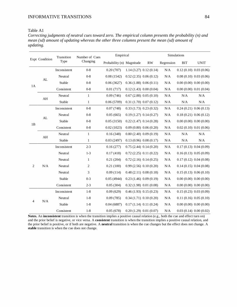
INFORMATIVE TRANSITIONS 84
Table A1
Correcting judgments of neutral cues toward zero. The empirical column presents the probability (n) and
mean (sd) amount of updating whereas the other three columns present the mean (sd) amount of
updating.
Expt Condition Transition
Type
Number of Cues
Changing
Empirical Simulations
Probability (n) Magnitude RW Regression BIT UNIT
1A
AL
Inconsistent 0-8 0.20 (707) 1.14 (3.27) 0.12 (0.14) N/A 0.12 (0.10) 0.03 (0.06)
Neutral 0-8 0.08 (1542) 0.52 (2.35) 0.06 (0.12) N/A 0.08 (0.10) 0.03 (0.06)
Stable 0-8 0.06 (3627) 0.36 (1.88) 0.06 (0.11) N/A 0.00 (0.00) 0.00 (0.00)
Consistent 0-8 0.01 (717) 0.12 (1.43) 0.00 (0.04) N/A 0.00 (0.00) 0.01 (0.04)
AH Neutral 1 0.09 (746) 0.67 (2.88) 0.05 (0.10) N/A N/A N/A
Stable 1 0.06 (5709) 0.31 (1.70) 0.07 (0.12) N/A N/A N/A
1B
AL
Inconsistent 0-8 0.07 (748) 0.33 (1.73) 0.23 (0.32) N/A 0.24 (0.21) 0.06 (0.13)
Neutral 0-8 0.05 (665) 0.19 (1.27) 0.14 (0.27) N/A 0.18 (0.21) 0.06 (0.12)
Stable 0-8 0.05 (3150) 0.22 (1.47) 0.14 (0.28) N/A 0.00 (0.00) 0.00 (0.00)
Consistent 0-8 0.02 (1023) 0.09 (0.80) 0.06 (0.20) N/A 0.02 (0.10) 0.01 (0.06)
AH Neutral 1 0.16 (348) 0.80 (2.40) 0.09 (0.19) N/A N/A N/A
Stable 1 0.03 (2497) 0.13 (0.96) 0.08 (0.17) N/A N/A N/A
2 N/A
Inconsistent 2-3 0.16 (277) 0.75 (2.44) 0.14 (0.20) N/A 0.17 (0.13) 0.04 (0.09)
Neutral 1-3 0.17 (418) 0.72 (2.25) 0.11 (0.22) N/A 0.16 (0.13) 0.05 (0.09)
Neutral 1 0.21 (204) 0.72 (2.16) 0.14 (0.25) N/A 0.17 (0.12) 0.04 (0.08)
Neutral 2 0.21 (100) 0.99 (2.56) 0.10 (0.20) N/A 0.14 (0.15) 0.04 (0.08)
Neutral 3 0.09 (114) 0.48 (2.11) 0.08 (0.18) N/A 0.15 (0.13) 0.06 (0.10)
Stable 0-3 0.05 (4944) 0.23 (1.46) 0.09 (0.19) N/A 0.00 (0.00) 0.00 (0.00)
Consistent 2-3 0.05 (304) 0.32 (1.98) 0.01 (0.08) N/A 0.00 (0.00) 0.00 (0.00)
4 N/A
Inconsistent 1-8 0.09 (629) 0.46 (1.93) 0.15 (0.23) N/A 0.15 (0.23) 0.03 (0.09)
Neutral 1-8 0.09 (785) 0.34 (1.71) 0.10 (0.20) N/A 0.11 (0.16) 0.05 (0.10)
Stable 1-8 0.04 (6887) 0.17 (1.14) 0.11 (0.24) N/A 0.00 (0.00) 0.00 (0.00)
Consistent 1-8 0.05 (678) 0.20 (1.29) 0.01 (0.07) N/A 0.03 (0.14) 0.00 (0.02)
Notes. An inconsistent transition is when the transition implies a positive causal relation (e.g., both the cue and effect turn on)
and the prior belief is negative, or vice versa. A consistent transition is when the transition implies a positive causal relation, and
the prior belief is positive, or if both are negative. A neutral transition is when the cue changes but the effect does not change. A
stable transition is when the cue does not change.
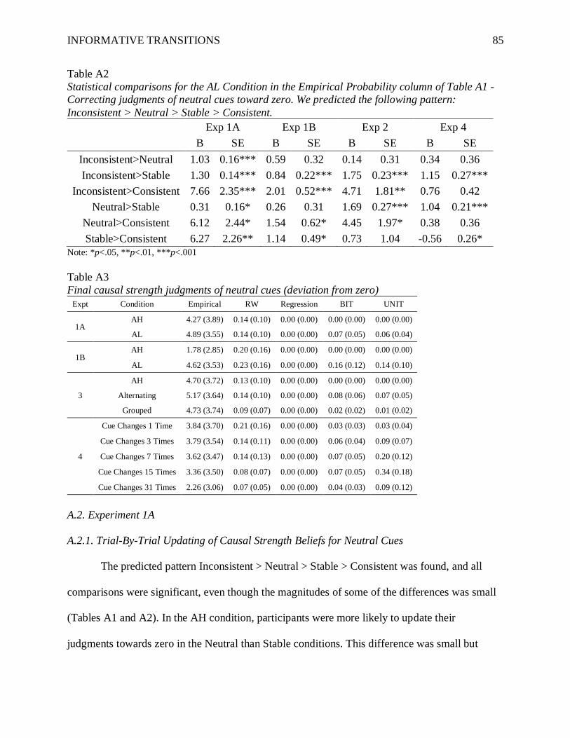
INFORMATIVE TRANSITIONS 85
Table A2
Statistical comparisons for the AL Condition in the Empirical Probability column of Table A1 -
Correcting judgments of neutral cues toward zero. We predicted the following pattern:
Inconsistent > Neutral > Stable > Consistent.
Exp 1A Exp 1B Exp 2 Exp 4
B SE B SE B SE B SE
Inconsistent>Neutral 1.03 0.16*** 0.59 0.32 0.14 0.31 0.34 0.36
Inconsistent>Stable 1.30 0.14*** 0.84 0.22*** 1.75 0.23*** 1.15 0.27***
Inconsistent>Consistent 7.66 2.35*** 2.01 0.52*** 4.71 1.81** 0.76 0.42
Neutral>Stable 0.31 0.16* 0.26 0.31 1.69 0.27*** 1.04 0.21***
Neutral>Consistent 6.12 2.44* 1.54 0.62* 4.45 1.97* 0.38 0.36
Stable>Consistent 6.27 2.26** 1.14 0.49* 0.73 1.04 -0.56 0.26*
Note: *p<.05, **p<.01, ***p<.001
Table A3
Final causal strength judgments of neutral cues (deviation from zero)
Expt Condition Empirical RW Regression BIT UNIT
1A AH 4.27 (3.89) 0.14 (0.10) 0.00 (0.00) 0.00 (0.00) 0.00 (0.00)
AL 4.89 (3.55) 0.14 (0.10) 0.00 (0.00) 0.07 (0.05) 0.06 (0.04)
1B AH 1.78 (2.85) 0.20 (0.16) 0.00 (0.00) 0.00 (0.00) 0.00 (0.00)
AL 4.62 (3.53) 0.23 (0.16) 0.00 (0.00) 0.16 (0.12) 0.14 (0.10)
3
AH 4.70 (3.72) 0.13 (0.10) 0.00 (0.00) 0.00 (0.00) 0.00 (0.00)
Alternating 5.17 (3.64) 0.14 (0.10) 0.00 (0.00) 0.08 (0.06) 0.07 (0.05)
Grouped 4.73 (3.74) 0.09 (0.07) 0.00 (0.00) 0.02 (0.02) 0.01 (0.02)
4
Cue Changes 1 Time 3.84 (3.70) 0.21 (0.16) 0.00 (0.00) 0.03 (0.03) 0.03 (0.04)
Cue Changes 3 Times 3.79 (3.54) 0.14 (0.11) 0.00 (0.00) 0.06 (0.04) 0.09 (0.07)
Cue Changes 7 Times 3.62 (3.47) 0.14 (0.13) 0.00 (0.00) 0.07 (0.05) 0.20 (0.12)
Cue Changes 15 Times 3.36 (3.50) 0.08 (0.07) 0.00 (0.00) 0.07 (0.05) 0.34 (0.18)
Cue Changes 31 Times 2.26 (3.06) 0.07 (0.05) 0.00 (0.00) 0.04 (0.03) 0.09 (0.12)
A.2. Experiment 1A
A.2.1. Trial-By-Trial Updating of Causal Strength Beliefs for Neutral Cues
The predicted pattern Inconsistent > Neutral > Stable > Consistent was found, and all
comparisons were significant, even though the magnitudes of some of the differences was small
(Tables A1 and A2). In the AH condition, participants were more likely to update their
judgments towards zero in the Neutral than Stable conditions. This difference was small but
INFORMATIVE TRANSITIONS 86
significant, B = -0.69, SE = 0.16, p < .001.
A.2.2. Final Causal Strength Judgments for Neutral Cues
The mean ratings of the neutral cues were near zero for both the AH (M = 0.92, SD =
5.70) and AL conditions (M = 1.01, SD = 5.97). Our main interest was whether the absolute
values of participants’ causal strength judgments were lower in the AH than the AL condition
(Table A3); the difference was in the expected direction but was not significant, B = -0.04, SE =
0.03, p = .16, R2 < .01, d = 0.14.
A.3. Experiment 1B
A.3.1. Trial-By-Trial Updating of Causal Strength Beliefs for Neutral Cues
In the AL condition, the findings again support the hypothesized pattern Inconsistent >
Neutral > Stable > Consistent, though the rates of updating towards zero were overall quite low
and the differences were small. (Note, the mean magnitude of updating in Table A1 shows a
stronger pattern than the probability of updates towards zero.)
In the AH condition there was considerably more correction back towards zero after a
neutral than a stable transition B = -2.03, SE = 0.41, p < .001. Also, fitting with the finding that
there is more updating of positive and negative cues in the AH than AL condition, there was
more correction of neutral cue after a neutral transition in the AH than AL condition (M = .16 vs.
M = .05), B = 1.58, SE = 0.35, p < .001.
A.3.2. Final Causal Strength Judgments for Neutral Cues
Participants’ final beliefs about neutral cues were closer to zero in the AH than in the AL
condition, B = 0.23, SE = 0.04, p < .001, R2 = .16, d = 0.86.
INFORMATIVE TRANSITIONS 87
A.4. Experiment 2
In Experiment 2, only the trial-by-trial updating was analyzed, not the final judgments,
because there was only one condition. The results generally followed the predicted pattern
Inconsistent > Neutral > Stable > Consistent; 4 of the 6 comparisons were significant (Table A2).
The main goal of Experiment 2 was to compare transitions during which one, two, or
three cues changed. Table A1 shows the probability of correcting toward zero after each kind of
transition, and also separates the neutral transitions according to the number of causes that
changed. A logistic regression with a by-subject random intercept and a by-subject random slope
for the number of cues changing found that subjects were marginally more likely to update their
judgments after a one-change than a two-change transition, B = -4.19, SE = 2.14, p = .05.6 There
was a significant difference between two-change and three-change transitions, B = 6.30, SE =
1.85, p < .001. The difference between the one-change and three-change transitions was in the
expected direction but was not significant B = -0.38, SE = 0.22, p = .09. Although some of these
individual comparisons were significant in the predicted direction, an overall analysis using the
number of changes (1, 2, or 3) as a random factor did not find a significant negative effect B = -
0.21, SE = 0.27, p = .45.
Our second analysis was coarser; we tested whether participants would correct toward
zero more often when fewer cues changed, across inconsistent, neutral, and consistent
6Though the means for the one-change and two-change conditions are the same in Table
A1, those means also include subjects who saw only a one-change or only a two-change
transition. The random effects model is especially sensitive to the subjects who saw both, which
provides an opportunity for a within-subjects comparison, which is how this result can be
marginally significant. In the subset of participants who saw both one-change and two-change
transitions the probabilities of correcting towards zero were .25 vs. .21, respectively. In the
subset of participants who saw both two-change and three-change transitions, the probabilities of
correcting towards zero were .17 and .09, respectively. In the subset of participants who saw
both one-change and three-change transitions, the probabilities of correcting towards zero were
.23 and .08, respectively.
INFORMATIVE TRANSITIONS 88
transitions; stable transitions were not included because we were only looking at transitions in
which a neutral cue changed. Our participants were more likely to correct a neutral cue back
towards zero after a single neutral cue changed (M = .21, N = 204), than after two cues changed,
at least one of which was a neutral cue (M = .12, N = 441), B = -0.67, SE = 0.34, p = .049. The
difference between two-change (M = .12, N = 441) and three-change transitions (M = .10, N =
354) was not significant, B = -0.24, SE = 0.39, p = .53. The difference between a one-change and
a three-change transition was significant, B = -1.01, SE = 0.43, p = .02.
In sum, there was more correction back towards zero for neutral cues when fewer cues
changed, though whether there is a significant difference between one vs. two cues changing, or
two vs. three, depends on the analysis.
RW captured the rough pattern of the effects. The IT models did not capture the expected
difference between one-change, two-change, and three-change transitions. Updating neutral cues
when multiple cues change can be very complicated and produce non-intuitive updating patterns.
For example, suppose that two neutral causes change, and suppose that one of the neutral causes
has a positive weight and another has a negative weight. Whichever cause has a stronger absolute
value of the weight will drive the error, and both cues will be updated in the same direction,
meaning that the cause that was previously believed to be weaker will actually be updated away
from zero.
A.5. Experiment 3
Only the final judgments were analyzed for Experiment 3. All three models predict the
causal strengths for the neutral cues to be very close to zero and for the absolute deviation to be
small (Table A3). They also do not predict large differences between conditions; BIT and UNIT
predict somewhat higher error in the Alternating condition because there are often multi-change
INFORMATIVE TRANSITIONS 89
transitions in which multiple cues (including neutral cues) change and the effect change. They
predict low rates of error for the grouped condition because the effect only changes once.
In fact, the absolute deviation from zero of participants’ strength ratings was slightly but
non-significantly higher for the Alternating condition. There were no significant differences
between the AH and Alternating Effect conditions (B = -0.01, SE = 0.02, p = .37, R2 = .003, d =
0.10), the AH and Grouped Effect conditions (B = 0.002, SE = 0.01, p = .92, R2 < .001, d < 0.01),
or the Grouped and Alternating Effect conditions (B = -0.01, SE = 0.01, p = .43, R2 = .002, d =
0.10).
A.6. Experiment 4
A.6.1 Trial-By-Trial Updating of Causal Strength Beliefs for Neutral Cues
Overall, the rates of correcting towards zero were quite low, so that even though the
effects were roughly in the expected directions, some were not significant. Two of the
comparisons were significant in the expected direction, and one in the unexpected direction
(Table A2).
A.6.2 Final judgments for neutral cues
Participants judged neutral cues that changed more to be weaker (more accurate), B = -
0.07, SE = 0.02, p < .001, R2 = .01, d = 0.24. This pattern fits with the pattern of learning about
positive and negative cues; positive and negative cues that changed more were judged as stronger
(more accurate).
RW captures this effect for the same reasons as it works for the positive and negative
cues. BIT and UNIT predict the most error for cues that change an intermediate number of times
(7), and lower error for cues that change few times (1) or many times (31). The reason for this
pattern is that if a cue changes very few times, there are very little opportunities for incorrect
INFORMATIVE TRANSITIONS 90
learning to occur (e.g., if a neutral cue changes at the same time as a positive cue, and the effect
also increases, which could make it seem as if the neutral cue is positive), so the cue weights stay
close to zero. In an intermediate amount of changes, there are a number of opportunities for
incorrect learning. After many transitions, the incorrect learning gets unlearned. The main
difference compared to participants is that when a subject learns about a cue that only changed
once instead of defaulting to assuming it is a neutral cue, they make a wide variety of judgments
with high error.