INFORMATION TO USERS - Yale Universityarb4/students_files/FengLiangThesis.pdfYale University in Candidacy for the ... For problems of model selection in regression, vve determine an

INFORMATION TO USERS

This manuscript has been reproduced from the microfilm master. UMI films

the text directly from the original or copy submitted. Thus, some thesis and

dissertation copies are in typewriter face, while others may be from any type of computer printer.

The quality of this reproduction is dependent upon the quality of the

copy submitted. Broken or indistinct print, colored or poor quality illustrations

and photographs, print bleedthrough, substandard margins, and improper alignment can adversely affect reproduction.

In the unlikely event that the author did not send UMI a complete manuscript and there are missing pages, these will be noted. Also, if unauthorized

copyright material had to be removed, a note will indicate the deletion.

Oversize materials (e.g., maps, drawings, charts) are reproduced by

sectioning the original, beginning at the upper left-hand comer and continuing

from left to right in equal sections with small overlaps.

Photographs included in the original manuscript have been reproduced

xerographically in this copy. Higher quality 6" x 9" black and white

photographic prints are available for any photographs or illustrations appearing

in this copy for an additional charge. Contact UMI directly to order.

ProQuest Information and Learning 300 North Zeeb Road, Ann Arbor, Ml 48106-1346 USA

800-521-0600

Reproduced with permission of the copyright owner. Further reproduction prohibited without permission.


Exact Minimax Procedures for Predictive Density Estim ationand D ata Compression

A Dissertation

Presented to the Faculty of the G raduate School

of

Yale University

in Candidacy for the Degree of

D octor of Philosophy

by

Feng Liang

D issertation Director: Professor Andrew R. Barron

May 2002


UMI Number: 3046185

___ ®

UMIUMI Microform 3046185

Copyright 2002 by ProQuest Information and Learning Company. All rights reserved. This microform edition is protected against

unauthorized copying under Title 17, United States Code.

ProQuest Information and Learning Company 300 North Zeeb Road

P.O. Box 1346 Ann Arbor, Ml 48106-1346


© 2002 by Feng Liang.

All rights reserved.


A b s tra c t

Exact M inim ax Procedures for Predictive D ensity Estim ation and

D ata Compression

Feng Liang

2002

For problems of m odel selection in regression, vve determ ine an exact m inim ax uni

versal data compression s trategy for the minimum description length (MDL) criterion.

The analysis also gives the best invariant and indeed m inim ax procedure for predic

tive density estim ation in location families, scale families and location-scale families,

using Kullback-Leibler loss. The exact m inimax rule is a generalized Bayes using

a uniform (Lebesgue measure) prior on the location param eter for location families

and on the log-scale for the scale families, and the p roduct measure on the com bined

location-scale families. Such im proper priors are m ade proper by conditioning on an

initial set of observations.

O ur proof for the m inim axity already implies the adm issibility for location families

in one dimension. However, it is well known th a t there m ight e;dst a bette r estim ato r

th an the constant m inim ax estim ator in high dimension. For example, for norm al

location families, the sam ple mean is not admissible when dimension is th ree or

higher (Stein, 55). Moreover, there exists a proper Bayes estim ator which is m inim ax

and produces be tte r risk everywhere than the sample m ean (Strawderman, 71), when


dim ension is bigger than four. We present an analogous result for predictive density

estim ation , using Kullback-Leibler loss.

2


Contents

1 I n t r o d u c t io n 3

1.1 Problem S ta te m e n t ............................................................................................... 3

1.2 Layout of This T h e s is ........................................................................................... 8

2 B e s t I n v a r ia n t E s t im a to r s 10

2.1 Location F a m il ie s .................................................................................................. 10

2.2 O ther Transform ation F am ilies ......................................................................... 13

2.3 Examples ................................................................................................................ 17

2.4 D isc u ss io n ................................................................................................................ 20

3 M in im a x E s t im a to r s 23

3.1 Location F a m ilie s .................................................................................................. 23

3.1.1 Proof for M in im a x ity ............................................................................. 24

3.1.2 A dm issibility and In a d m is s ib il i ty ..................................................... 26

3.2 O ther T ransform ation F am ilies ......................................................................... 28

3.3 M inimal Conditioning S i z e ................................................................................ 33

3.4 M inimax Rule For R e g re s s io n ......................................................................... 35

3.5 A p p e n d ix ................................................................................................................ 40

4 A P r o p e r B ay es M in im a x E s t im a to r 44

4.1 In tro d u c tio n ............................................................................................................ 44

1


4.2 M ain Result and P r o o f ......................................................................................... 45

4.3 Im p lic a tio n s ............................................................................................................ 51

4.4 A p p e n d i x ................................................................................................................ 53

2


Chapter 1

Introduction

Suppose we observed some data from a normal d istribu tion w ith standard variance

and unknown m ean. So what is a good density estim ato r for the next observation?

Of course, I should first define what I mean about a good estim ator.

1.1 P ro b lem Statem ent

Let Y — ( Yi , . . . , Yn) be a random vector to which we wish to assign a distribution

given observed d a ta Y — (Yi , . . . , Ym). For each model it is assum ed th a t there is a

param etric fam ily of distributions PY\g and Py\Y0 densities p(y | 6) and p(y \y ,9 ) ,

depending on a d-dimensional param eter vector 6 taking values in a param eter space

0 , possibly consisting of all of To each choice of predictive distribution Q Y\Y with

density q{y | y) we incur a loss given by the Kullback-Leibler inform ation divergence

d (p y\y,6WQy\y) = J p(v 1 v-.d) lQg p( ~ j/~ p dv- ( i - i )

Our in terest is in the minimax risk

R = mQin *20- Er\9D (PY\Y,eWQY\Y) (!-2 )

and in the determ ination of a predictive d istribution Q Y \Y th a t achieves it. In uni

versal d a ta compression [23][5], the value \ o g \ / q ( y \ y ) corresponds to the length of

3


description o f y given y in the absence of knowledge of 9, and the expected Kullback-

Leibler loss arises as the excess average code length (redundancy)

E ^ , , [log l / l ( Y I Y ) - log l / p ( Y I V, 0 )

The op tim al choice of q(y | y) is the one providing the m inimax redundancy.

In th is thesis, I provide exact solution to this m inimax problem for certa in families

of densities param eterized by location or scale. Implications are discussed for predic

tive density estim ation and for the M inim um Description Length (MDL) criterion.

D en sity E stim a tio n

In density estim ation , our aim is to estim ate the density function for Y using the data

Y in the absence of knowledge of 9. The risk function is the expected Kullback-Leibler

loss R(9,q) = Ey|flD (Pp|0 ||Qy>|K). E stim ato rs q(y | y) are required to be non-negative

and to in teg ra te to one for each y, and as such can be in terp re ted as predictive

densities for y given y. Though it may be custom ary to use plug in type estim ators

q(ij I y) = P(y I &(y))i one finds th a t the op tim al density estim ators (from Bayes and

m inim ax perspectives) take on the form of an average of members of the fam ily with

respect to a posterior distribution given y. We remind the readers of th e Bayes

optim ality property : w ith prior w and Kullback-Leibler loss, the Bayes risk Rw(q) =

f R (9 , q)w(9)d9 is minimized by choosing q to be the Bayes predictive density

I - 1 x f m f e p (y ,y \0 )w (9 )d 9p M \v) = j p (v I v, S M S I y)M = J&p(l)lg)w{e)M ■ U-3)

Indeed for all q the Bayes risk difference Rw(q) — Rw(pw) reduces to the expected KL

divergence betw een pw and q which is positive unless q = pw.

A procedure is said to be generalized Bayes if it takes the sam e form as in (1.3),

with a possibly im proper prior (i.e. f w{6)d9 might not be finite), b u t proper pos


terior. Such generalized Bayes procedures arise in our exam ination of m inim ax opti

mality.

I prove th a t for location families w ith Kullback-Leibler loss, a m inim ax procedure

is the generalized Bayes using a uniform (Lebesgue) prior. A sim ilar conclusion holds

if for a un ivaria te scale param eter 0 ^ 0 such th a t K = 9~l Zi where now the m inim ax

procedure uses a uniform prior on lo g |0 |. Likewise when one has bo th m ultivariate

location (01 E Rd) and univariate scale (02 / 0 ) param eters such th a t Yt = O ^ Z i + 01?

the m inim ax procedure uses Lebesgue product measure on 0\ and lo g |0 2|.

P artia l resu lts (showing the procedure th a t minimizes risk am ong invariant esti

m ators) are given for families defined by o ther groups of transform ations including

linear transform ations K = d~lZ { for d x d non-singular m atrices 0 and affine trans

form ations Yi = 02*1 Z{ 4- 0i where 0i E 02 is non-singular d x d m atrix . The

best invariant density estim ator uses the prior l / \6 \d (where |0 | denotes the absolute

value of the de term inan t of m atrix 0 ) for linear transform ation families, and the prior

1 / 1 21 ( w i t h respect to Lebesgue product measure on the coordinates of 0X and 02)

for affine families.

For norm al location families, I give a proper Bayes estim ator which is m inim ax and

produces sm aller risk everywhere than the constant m inim ax estim ator. This work

is related w ith S traw derm an’s [22] proper Bayes estim ator for m ultivaria te normal

mean vector.

M in im u m D escr ip tion L en gth

Of particu lar h istorical and practical im portance is the problem of m odel selection in

linear regression, first considered from the MDL perspective by Rissanen [16]. Suppose

we have a to ta l o f N observations K which m ay be predicted using given d-dim ensional

explanatory vectors x* for i = 1, 2 , . . . , N . One may describe such outcom es using a

5


Gaussian d istribution , in which for given 0 and a 1, each Yt is m odeled as independent

N orm al(x‘0, a 2) for i = 1 , 2 , . . . , N . If a 2 is fixed and 0 is estim ated , these models

lead to description length criteria of the form

2^5 5 1 ^ * ' “ x & 2 + ^ log AT + c.i = 1

In Rissanen’s original two-stage code form ulation, the param eter 0 is estim ated by

least squares and the term ( | log N + c) corresponds to the length of description of

the coordinates of 0 to precision of order l / \ / N . Various values for c have arisen in

the literature corresponding to different schemes of quantification of 0 , or to the use

of m ixture or predictive coding strategies ra th er than two-stage [19]. A sym ptotics in

N have also played a role in justifying the form of the criterion [5]. W hen several

candidates are available for the explanatory variables x, the model selection criterion

picks out the subset of the variables th a t leads the shortest to ta l descrip tion length

achieving the best trade off between sum of squared errors and the com plexity of the

model (d/2) log N -I- c.

In this thesis I show th a t if one conditions on m initial observations w ith m at

least as large as the param eter dimension d, then for any regression problem and for

all prediction horizon lengths n > 1, an exact m inim ax strategy is to use a m ixture-

based code (or predictive distribution) where the prior is taken to be uniform over

0 in (made proper by conditioning on the initial observations). As a particu lar

case of the general theory, the exact m inim ax strategy for linear regression models

w ith Gaussian errors is studied. The exact m inim ax strategy leads to the description

length criterion of the form1 N i iV

2^2 ~ x i8ff)2 + 2 log I XiXi\ ~i = I i = 1

where I specify the exact form of Cm (it is YJT= \.(yi-x \dm )2+ | log | Xix[|).

If we set R n = j j x ix b then the m ain term s in the penalty are ^ lo g A - +

6


jlog |i?yv|. For some Xj-’s (e.g. those evolving according to some no n sta tio n ary time

series m odels), th e sum YliLi x ix \ may grow a t faster rates, e.g. o rder N 2 ra th e r than

N , leading to \ log \ N R n \ of order d logiV ra th er th an | log N . In general it is better

to retain the i log |iV/?jv| determ inate form of the penalty ra th e r th a n the |lo g iV .

Thus the de term inan t of the inform ation m atrix plays a key role in the

exact m inim ax s tra teg y for regression. Previous work has identified the role of the

inform ation m atrix in asym ptotically op tim al two-stage codes [2], in stochastic com

plexity (Bayes m ix tu re codes) [2][18][3] and in asym ptotically m in im ax code [4][20]

when the p aram eter space is restricted so th a t the square root of th e determ inant of

the inform ation m atrix is integrable.

Priors providing asym ptotically m inim ax codes in [4] are m odifications of Jef

freys’ prior (p roportional to the root of th e determ inant of the inform ation m atrix),

historically im p o rtan t [13] [11] because of a local invariance p roperty - sm all diame

te r K ullback-Leibler balls have approxim ately the same prior probability in different

parts of the p aram eter space. For the regression problem and o th er unconstrained

location and scale families the Jeffreys’ prior is im proper (root d e term inan t informa

tion is not integrable) com m ensorate w ith infinite m inim ax redundancy. Nevertheless,

conditioning on sufficiently many initial observations produces p roper posterior dis

tributions and finite m axim al risk (conditional redundancy). C onditioning on initial

observations can change the asym ptotically op tim al prior from w hat it was in the

unconditional case. In particular, w ith conditioning, the optim al p rio r need not be

Jeffreys’. Nevertheless, the procedures we show to be exactly m inim ax (w ith condi

tioning) do coincide w ith the use of Jeffreys’ prior for location or scale families.

7


1.2 L ayout o f T h is T hesis

This d isserta tion is arranged as following:

the problem has already form ulated in section 1 in this C hapter. Im plications like

density estim ation and model selection are also discussed. I do not have a “historical

review” in th is Chapter, instead I will discuss those related work in each Chapter.

In C h ap ter 2, I am going to introduce a class of estim ators which are invariant

under certain transform ations such as location shift. One property of invariant esti

m ators is th a t they have constant risk. The best invariant estim ators are calculated

for some transform ation families such as location families. Exam ples for some famil

iar param etric families are given. The understanding of invariance th rough groups of

transform ations and the connection between best invariant estim ators and right Haar

m easure are given in the discussion section.

In C hap ter 3, I prove th a t the best invariant estim ators are m inim ax for location

families, scale families and the m ultivariate location and univariate scale families,

if conditioning on enough initial data . The minimax risk is instead infinity if not

conditioning on enough d a ta set. The proof for m inim axitv already implies the ad

m issibility in one dimension. For norm al location family, I find th a t the constant

m inim ax estim ato r is not adm issible when dimension is three or higher. The simi

lar analysis reveals the m inim ax estim ator for regression under K ullback-Leibler loss.

Consequently, we can use such a m inim ax estim ator to derive a criterion for model

selection in regression.

The m inim ax estim ator, which is also the best invariant estim ato r w ith constant

risk, is a generalized Bayes estim ator w ith the im proper uniform prior on location

param eter for location families. In C hapter 4, for normal location family, I will give

a proper Bayes estim ator which is also m inim ax and produces b e tte r risk everywhere

8


than the constant minimax estim ator, provided th a t the dimension is bigger than

four. This piece of work is related w ith Straw derm an’s proper Bayes estim ator in

point estim ation for normal location.

9


Chapter 2

Best Invariant Estimators

2.1 L ocation Fam ilies

Consider first location families. We are to observe Y = (V'i, . . . , Fm) and want to

encode or provide predictive d istribu tion for the future observations Y = (V'i, . . . , Yn),

where Yi = Zi + 9, Y{ = Zi + 9 w ith unknown 9 e Rd. We assum e th a t Z =

( Z i , . . . , Zm) and Z = ( Z i , . . . , Z n) have a known joint density p z z . Then the jo in t

density for Y and Y is given by p(y, y | 9) = pz z {]J — 0, V — #)• We use y — 9 and

y — 9 as shorthand notations for yi — 9, . . . , — 6 and yi — 9 , . . . , yn — 9, respectively.

W hen the context is clear, we will w rite p z z as p.

Our first goal is to find the best invariant estim ator or coding s tra teg y q*(y | y).

D e fin itio n 1 A procedure q is invariant under location shift, i f fo r each a € and

all y, y, q(y \ y + a) = q(y — a \ y ) .

T hat is, adding a constant a to the observations y = ( y i , . . . , ym) shifts th e density

estim ator for y by the same am ount a. Consequently, if we shift bo th y and y by the

same am ount, the value of q{y | y) is unchanged,

q(y + a |y + a) = q ( y \ y ) . (2 .1)

P r o p o s i t io n 1 Invariant procedures have constant risk.

10


P ro o f : A pplying the invariance of q, we obtain

R(9 ,q) = E y y , 0\o g P^ ~ ~ 6>) = Ez z l o g P(f . (2.2)' ^ ' r,g h q { Y - e \ Y - 6 ) ZZ % ( Z | Z ) 1 '

which is equal to R(0,q), a quantity not depending on 0. T hus P roposition 1 is

proved. □

Now we derive the best invariant procedure. The idea is to express the risk in

terms of transform ed variables th a t are invariant to the location shift: here Zj — Zi,

Zi — Z\ for j = 1, . . . , n and i — 2 , . . . , m . Applying the invariance property (2.1)

with a = —Zi in equation(2.2), we ob tain

R{B,q) = Ez log — =---------------P(Z \ Z)--------------------z,z q(Z — Z x | 0, Z2 — Z 1; • • • , Zm — Zi)

Define U = Z — Z\ , U\ = Z]_ and Ui = Zi — Z\ for i = 2 , . . . . m. Then U given

U2, ■ ■ ■, Um will have a conditional density function p(u \ u2, , u m) which we show

provides the op tim al q. Indeed for any q , the risk satisfies

p ( Z | Z )R(d, q) = Ez z log

q ( U I 0, C/2, • • • , Um)

> Ez,z log - f f 1 z) (2.3)p(U \ U2, . . . , U m )

because the difference

E log , 6 '2------ Um) = Et ,„ log p{? 1 °'2'- ' • ’ ° m) ]& q ( U \ 0 , U 2, . . . , U m) ....“ - 1 U,U‘ U~ q(U I 0 . LT2-. ■ • • : Ujn)

is an expected Kullback-Leibler divergence th a t is greater th an or equal to zero, and

it is equal to zero (i.e. achieves the sm allest risk) if and only if q{u | 0, u 2, . . . , um) =

p ( u \ u 2, . . . , u m ) -

This analysis for the best invariant density estim ator w ith K ullback-Leibler loss

is analogous to th a t originally given by P itm an [15] (cf. Ferguson [10], page 186-187)

for finding the best invariant estim ator of 6 w ith squared error loss.

11


Now we solve for p(u | u 2, . . . , u m) — p(u2, . . . , um, u ) /p ( u 2, . . . . ttm). Note th a t the

m apping from Z , Z to U, U has unit Jacobian. So the jo in t density p(u, u) is given by

P2 z {uuU2 -f u i , . . . , um + «i , u 4- «i). Integrating out u l: we obtain

p(u2, . . . , um, u) = J p z z ( u i , U 2 + U i , . . . , U m + U i , U + U i ) d U y . (2.4)

Observe th a t Ui = Zi — zi = yi — y i for i = 2 , . . . . m and u = z — Zy = y — y 1: then

(2.4) is equal to

j P z , z ( U h V2 - V i + u h ■ ■ ■ i V m - y \ + M l , y - IJl + U ^ d U y .

Letting 9 = yy — uy, we m ay express this integral as

J Pz ,z (y i - 0 ^ y 2 - 9 , . . . , y m - 9 , y - 9)d0 = J p ( y , y | G)d9.

Similarly, we obtain p(u2, . . . , um) = f p(y \ 9)d9. Thus the conditional density for u

given u2, . . . , um (expressed as a function of y and y) is the ratio,

/ - i \ f P i V i y I 9)dQp ( u \ u 2, . . . . u m) = f p { y l e ) d e , (2 .5 )

which we denote as q*{y | y). One can check th a t q* is an invariant procedure under

location shift. O ur analysis a t inequality (2.3) and following show th a t this predictive

density q* has the sm allest risk am ong all invariant estim ators. It is also the unique

best invariant one due to the stric t convexity of the KL loss. So we get the following

proposition.

P r o p o s i t io n 2 The unique best invariant predictive density fo r a location family is

f p ( y , y \ 0 ) d 0, ( , l s ) = 7 * w T ^

12


The procedure q* we have showed to be the best invariant can be interpreted as

a generalized Bayes procedure with uniform (im proper) p rio r w(9) constant on K.d

(Lebesgue measure) for location families. Bayes prediction densities are not invariant

in general, except for certain im proper priors, identified in H artigan [11] as relatively

invariant priors, for which w { 9 Jr t ) = c(t)w(9), e.g., w(9) = cea0. A corollary then of

Proposition 2 is th a t the relatively invariant prior w ith th e sm allest constant risk is

the uniform prior on Rd {w{6) — c).

2.2 O ther T ransform ation Fam ilies

Sim ilarly we can derive the best invariant predictive density estim ato r for other trans

form ation families, such as

1. Linear Transform ation family: Yi = 9~lZi, Y = 9~lZi, where 9 is a non-singular

d x d m atrix and

p(y,y I#) = \9\m+npZ'z(9y,9y)Specially, when d = 1, it is called a univariate scale family.

2. Affine family: Yi = 9 f l Z{ 4- 9X, Y = 9 ^ xZi + 9^. G 92 non-singular d x d

m atrix

p { y , y \ e ) = \92r +nPz^{9 2{y - 9 ^ , 9 ^ - 9X))

3. M ultivariate location w ith univariate scale: same as in affine family with 9\ G

but with scalar 92 G R — 0.

p(y, &\0) = l«2l lm+,'v pz.i m y - e,), e2(y- t>, ))

D e f in i tio n 2 A procedure q is invariant under linear transformation i f for any non

singular d x d matrix b and all y, y, q(y | by) = j ^ q ( b ~ ly | y). Thus

\b\nq(by j by) = q(y | y). (2 .6 )

13


It is invariant under affine transformation i f f o r any a G Rd and non-singular d x d

matrix b,

W q { b { y - a) | b(y - a)) = q(y | y). (2.7)

Likewise, it is invariant fo r multivariate location with univariate scale i f f o r any

a 6 K.d and non-zero scalar b,

\b\ndq(b(y - a) | b{y - a)) = q(y | y). (2 .8 )

Suppose q is invariant under linear transform ation, then the risk R(0, q) is equal

to

^ 1 \9\nq { 9 Y \0 Y ) ' q ( Z \ Z )Thus q has constant risk. Similarly, the risk is constant for affine transform ation

families and affine invariant estim ators. Likewise, for m ultivariate location w ith uni

variate scale families. A parallel result to P roposition 2 is given below for the three

families.

P r o p o s i t io n 3 The unique best invariant predictive density is

, /© w P (V i V I d ) d e

q (y\y> = ~ r i —I Ta\â~f e JopP(y I ®)ddfor a linear transformation family,

, /© iflq*p(y, y I 0)d0q ( y I y >= ~i— / i n ^ ,Q

f e m p p ( y l ° ) ddfor an affine family where dQ denotes integration with respect to both location param

eter Qx in and scale parameter 02 in Rdxd, and

, f e j k p ^ y ^ y i ° )dB q (y\y) = t M —, im.a-f e m p (y 19)dd

for a multivariate location with univariate scale family, where dO denotes integration

with respect to both the location parameter 0X in and the scale parameter d2 in

R - {0 }.

14


P ro o f: As we stud ied before, for all three transform ation families, we have the

risk R{Q,q) equal to

Ewlog^fHf (2 '9)q { Z \ Z )

For linear transform ation , let Z f denote ( ZL, . . . , Zd)-. the d x d m atrix w ith Z, in

the zth column for i = 1 , . . . , d. Define

U = ( Z ? ) - lZ, Ui = ( Z f ) - lZI7 i = d + l , . . . , m . (2.10)

N ote th a t those variables are invariant to linear transform ation of the Zt and Z , so

th a t

U = { Y ? ) ' lY , Ui = { Y f Y 'Y i , i = d + 1, . . . , m, (2 .11)

where Y f is the d x d m atrix formed from the initial portion of Y.

Applying the invariance property (2.6) in (2.9) w ith b = ( Z f ) _I , then in a m anner

sim ilar to the proof for location families (Proposition 2), the best invariant estim ator

q* satisfies

qm{ u \ e u . . . , e d, ud+i,m) = P(^ +l ’m, f , (2 .12)P{u d+l,m)

where e* is the zth colum n of the d x d identity m atrix and u d+ i,m = (ud+l, . . . , um).

Next we derive the expression (in terms of y and y ) for bo th sides of (2.12). By the

m apping between U, U and Z, Z given in (2.10), the jo in t density for Z \ . . . . , Z d, Ud+ i,m

and U is given by

\z l |m+ Pz,z(Z 1: ■ ' ' Zdi z \ ud+1? - • • i z l UTn-> z l &).

where \zf\ denotes the absolute value of the determ inant of the m atrix z f and |zji |7n+n-d

comes out as the Jacobian. Rewriting ud+ itm and u using (2.11) and changing the

variables of integration z f = (21, . . . , zd) to 6 = 2f (yf ) - 1 , a d x d m atrix, we obtain

p(u«i+ifm,w) = | v i\n+rn J p ( y , y \ Q) d 0 .

15


Then the conditional d istribu tion is equal to

I vid ,n fp ( y ^ y \d)de

f p { y \ 9 ) d d

O n the other hand, using the equalities at (2.11) and the invariance p roperty of q*,

we have the left side of (2.12) equal to \yi\nq*[y1 y ). So

S p ( y , y \ o ) d 9 = f P(yW e •

For the affine families, define the variables

0 = \ Z p l - Z X\ \ - \ Z - Z x), Ui = \ Z i * ' - Z x\ \ - ' ( Z i - Z x), i = d + 2 , . . . , m ,

(2.13)

where 1 = (1, . . . , 1) is the row vector of all one’s and thus Z \ \ is the m atrix w ith

d identical columns Z\. One can see th a t the variables U and £/, are invariant to

affine transform ation of the Z /s and Z. Applying the invariance property (2.8) w ith

a = — Z\ and b = [Z$ — Z i l ]-1 in (2.9), we find the best invariant estim ator q* satisfies

q*{u | 0, e l5. . . , erf, u d+2,m) = p{u | Ud+2,m)- The rem ainder of the proof is the sam e as

the one above for the linear transform ation families.

For m ultivariate location w ith univariate scale families, define a scalar random

variable W which is the first coordinate of the vector Z2 — Z\. The last d — 1

coordinates divided by W is defined to be V (thus (1, V) = (Z2 — Z \ ) / W ) and we

define

& = (2.14)

A fter applying the invariance property with a = —Z\ and b = 1/HA it tu rn s out

th a t the best invariant estim ato r q* satisfies q*(u | 0, (1, v), u^^m) = p(u \ v, The

jo in t density for V, C/3im and U is given by

J |ry|(m+n_I)<i_lp Zj^ (2i, (w , wv) + Z\ , w u 3 + z i , . . . , w u m -I- z t , wu + z\)dz]_dw. (2.15)

16


Let b be the first coord inate of vector Y2 — Yi. Note V , U and C/t ’s are invariant to

location shift and univaria te scale, th a t is, V is equal to the last d - 1 coordinates of

Y> — Yi divided by b and

fr * - Y l rr K - Y .t . „U = ---- , Ui = ---- ------, I = 3 , . . . , m.

Plug them back into equation (2.15) and change variable w to 02 with w = 02b, then

(2.15) is equal to

J |02 |(m+n_I)rf-1|&|(m+" " 1)dP£,;z(zi, 02(z/2- J / i )+ z i , • • •, 02(z/m -I/i)+ zi, 02( y - y i ) + z i ) d z i d d 2.

Change variable again w ith Q\ = — z i /0 2 whose Jacob ian is \02\d to obtain

The rest of the proof is th en the same as we have given for o ther transform ation

families. □

2.3 E xam ples

The best invariant es tim ato r q* is calculated for some exam ples in which we have m

observations Y i , . . . , Ym and w ant to estim ate the density for the next observation Y .

Let Y(i) be the i th order s ta tis tic (the zth smallest value) am ong Y \ , . . . , Ym.

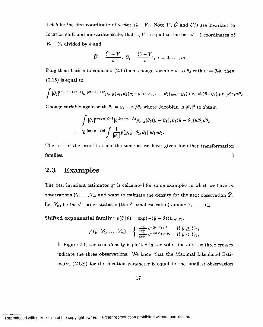
S h if te d e x p o n e n t ia l f a m ily : p(y | 0) = exp (—(y — 0 ) ) l { y>o>.

n*hl IV, y u m+l y — (!)q {.y\ | _ ^_ e-m (r(1)-y) i f y < y (1)

In Figure 2 .1, the tru e density is plotted in the solid line and the three crosses

indicate the three observations. VVe know th a t the M axim al Likelihood E sti

m ator (MLE) for th e location param eter is equal to the smallest observation

17


true density

&■aceo

0.5 t.O 15 2 52.0 3.0

Figure 2.1: P lo t of true density vs. q* for shifted exponential family.

V(p. The corresponding MLE plug-in estim ator for the density is plotted in the

dash-dot line. We can see there is a gap between the true density and the MLE

plug-in estim ator, which causes infinite loss. Some calculations reveal th a t the

best invariant estim ato r q* has finite risk equal to log (l -+- T ). To avoid the in

finite loss, the best invariant estim ator q*. p lo tted in the dashed line in Figure

2 .1, d istributes a sm all portion ( ^ j ) of the to ta l m ass on the left of and

puts the rem aining mass on the right. This is an exam ple in which the opti

m al (best am ong invariant estim ators) estim ator is not in the same param etric

family as the tru th .

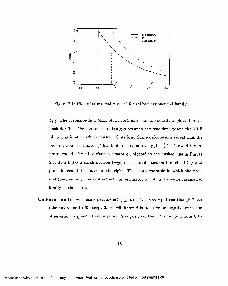
U n ifo rm fa m ily (w ith scale param eter): p(y | 9) = |0|l{o<oy<i}- Even though 9 can

take any value in R except 0, we will know 9 is positive or negative once one

observation is given. Here suppose Y\ is positive, then 9 is ranging from 0 to

18


tru e d e n s i ty q* w ith m = 5

1-1.5

Figure 2.2: Plot of true density (0 = 1) vs. q* (m = 5) for uniform family with scale param eter.

oo.

' 1 f p ( Y u . . . , y m \ e ) l M

if g > v'(m,

Figure 2.2 plots the tru e density (solid line) and the best invariant estim ator q*

(dashed line) for 6 = 1 and m = 5.

N o rm a l L o c a tio n : Norm al(0, cr2), 0 unknown and a 2 fixed wi thp(y | 0) = 0^2 ( y —0).

qm( y \ Y u - - - : Y m) = 0 <T2(1+ x )(y - V').v 771

This is the norm al density w ith mean Y = (1/m ) Yi and a slightly larger

variance cr2( l + L ). The MLE plug-in estim ator, a norm al density w ith mean

Y , but variance cr2, is also invariant. The risk for the MLE plug-in estim ator is

equal to ( f ) ( ^ ) , which is bigger than the risk of q“, ( | ) log(l -I- T).

19


N o rm a l lo c a tio n a n d sc a le : Norm al(0. cr2). 9 £ Rd, a 2 > 0, both unknown. T he

best invariant estim ato r is proportional to (1 + ||y — y ||2/ s 2c)-md/2, th a t is

a - t i w Y ) r ( ^ > + 1 i i y - * T , n - ^" , l r ( (m; 1>1' ) [ir{m - l)d]d l (m - l ) c / (1 + l / m ) i 2 J

where s2 = 52™. t ll « — ^"ll2/ ( ( m ~ 1)* ) is the sam ple variance. Thus T = (V' —

h ) /[ ( ! + m)^2]l/2 assigned a predictive d istribu tion which is the m ultivariate

t d istribution with (m — l)d degrees of freedom.

U n ifo rm o n P a ra l le lo g ra m s : p(y |0i ,0o) = {0-21l(o,i)x(o,i)(^2(2/ + 0 i ) ) , where e

R2 and 02 is a 2 x 2 m atrix w ith determ inant not equal to 0 . Conditioning on a t

least three observations, one can show th a t the best invariant density estim ation

q ' is constant in the convex hull spanned by the observations, and tapers down

toward zero as one moves away from the convex hull.

2 .4 D iscussion

In this section, we will briefly review some results abou t invariant decision problem s

through groups of transform ations. For more detail, please refer to [9][25][6].

In a decision problem, we have a sam ple space X . a family of densities with

param eter space 0 and an action space A . Suppose there is a group of transform ations

(one-to-one and onto) G on the sam ple space, th a t is, all the transform ations from G

form a group using the usual composition as the group operator.

The param eter space is said to be invariant under the group G i f , for every g £ G

and 8 £ 0 , there exists an unique 6' £ 0 such th a t the corresponding density for

g{Y ) is p { y \6 ' ) . We can denote 9* by g(9), then G = {g : g £ G } is the induced

group of transform ations on 0 into itself. Consequently, the following two equalities

hold true:

P0(g (X ) £ A) = Pm ( X £ A)

20


and

E»[/(S(-Y))] = I W /( -Y ) ] .

A loss function L ( 6 ,a ) is said to be invariant under the group G if , for every

g £ G and a £ A , there exists an a* £ A such th a t L(6. a) = L{g{9), a*) for all 0. The

action a* is denoted by g(a), and then G = {g : g £ G } is a group of transform ation

of the action space A into itself.

Now we restate some of the invariant decision problems we considered in this

C hap ter using the idea of transform ation groups.

E x a m p le 1 For location fam ily with X = Kd. consider the transform ation group

G = {gc : c £ Kd }. where gc{x) = x + c. This group is called th e additive group or

location group. The corresponding transform ation on the p aram eter space is gc(6) =

Q + c, and the one on the action space is gc(q) = q(y — c: y), since

. p (V ' | y ,0 + c)L{gc{9)-gc{qy\y)) = Ey-|0+clog

= % --c |0 log

= E.y|0 log

q (Y - c; y) p{Y — c \ y , 9 )

q{Y - c: y ) p {X \y .O )

= L[0,q),

where we change the integration variable Y' — c to X a t the th ird equality. So this

decision problem is invariant under the location group.

E x a m p le 2 For an affine fam ily with X = R, consider the transform ation group

G — {gb,c{%) = bx + c. b £ M.. c £ K.}. It can be checked th a t the decision problem for

the affine fam ily is invariant under th a t group.

Next we give the definition of right H aar density.

D e f in i t io n 3 A density vr is a right Haar density on G i f fo r any set , 4 g G and all

21


<7o C G, it satisfies

Similarly, we can define left H aar density (measure).

For example, the uniform is the right Haar measure for the location group since

if we shift a set A to A + c, its measure is unchanged.

The best invariant estim ators, we identified in this C hapter, are generalized Bayes

estim ators w ith im proper priors which are made proper by conditioning. Those im

proper priors are the same as the right H aar measures for the corresponding transfor

m ation groups on the param eter space 0 which leave the decision problem invariant.

This is not a coincidence. It is proved th a t under some conditions the best invariant

estim ator is the generalized Bayes estim ator using the right Haar measure (Berger

[6]). The calculations in Section 1 and 2 in this C hapter, which follow P itm an’s

technique, provide a way to understand this general result w ithout any knowledge of

group theory.

22


Chapter 3

Minimax Estimators

Since the risk is constant for invariant predictive density estim ato rs, the best invariant

estim ator q* is the m inim ax procedure among all invariant procedures. Hunt-Stein

theory provides a means by which to show that under som e conditions the best

invariant rule is in fact minimax over all rules, and this s tra teg y has proved effectively

in param eter estim ation and hypothesis testing [24][14], T he sam e technique might

be carried over to prove the same conjecture for predictive density estim ation. In

this paper, we provide a proof based on the fact from decision theory th a t constant

risk plus extended Bayes implies m inim ax (see A ppendix A). We use tools from

Inform ation Theory to confirm th a t our best invariant procedure, which is known to

have constant risk, is extended Bayes and hence minimax.

3.1 L ocation Fam ilies

We first work w ith location families. Recall a location fam ily has observations Y\ =

Zi + 9 w ith i = 1 , . . . , m and future d a ta Yj = Zj + 9 w ith j = 1, . . . , n, where 9

is unknown and we assume Z = ( Z i , . . . , Z m) and Z = ( Z j , . . . , Z„) have a known

joint density p z z - Then the jo in t density for Y' and Y' is given by p(y, y \9) =

P z j i y - Q , y - 6 ) -

23


3 .1 .1 P r o o f for M in im ax ity

D e f in i t io n 4 A predictive procedure q is called extended Bayes, i f there exists a se

quence of Bayes procedures {pWk } with proper priors Wk such that their Bayes risk

differences go to zero, that is,

Rwk{q) - Rwk(,Pwk) -> 0 , as k -» oo.

T h e o r e m 1 Assume for the location family that at least one of the Z \ , . . . , Z m has

f inite second moment. Then, under Kullback-Leibler loss, the best invariant predictive

procedure\ f p ( y , y \ 9 ) d 0

q ( y \ y ) = r t iJ p(y Io)deis m in im ax fo r any dimension d.

P ro o f : To show minimaxity, it suffices to show th a t qm, known to have constant

risk, is extended Bayes. We take a sequence of priors to be the normal d istribu

tions w ith mean zero and variance k. Recall th a t the corresponding Bayes predictive

procedure pWk is defined by (1.3).

Exam ine the Bayes risk difference between q* and pWk.

Rwk(q') - RWk{Pwk) = J [R(9,q') - R(0,pWk)]tVk(9)d9

= Ey- y log Pwk (3

where in the expectation E yy-, the distribution of (T , 1 ) is a m ix tu re with respect to

p rio r w k.

By the chain rule of Inform ation Theory, the Bayes risk difference

Ey-,'- lOg ^ C?" I*l» - • • ’ *"«)( K i l l , . . . , I'm)

24


is less than or equal to the following to tal Bayes risk difference (conditioning only on

Yi).

e ^ o

_ r f p ( Y \ : . . . , Y m. Y \ 9)wk( 9 ) ^ d 9 J p { Y x \9')wk{9')d9'

° g f p ( Y u . . . , Y m, Y \ 9 ) w k(9)d9 ° S f p ( Y x \9')d9' J

= Ey-,r [ - logE0|V-,-.(— L y ) - log j p ( Y x | 9')wk(9')d9']

where we have used th a t f p ( Y x | 9')d9' = 1. The variable on which to condition is

chosen to be one for which the variance is finite (here F1; w ithout loss of generality).

Invoking Jensen's inequality in both terms (using convexity of — log), we get the

Bayes risk difference is less th an or equal to

Efl log wk{9) - Ey-j J p ( Y \ I 9') log Wk(9’)d9'

= j ' wk(9) lo g wk(9)d9 - J J w k{9)p{yx - 9)p{yx - 9') log ^ ^ ^ dO'dy^9(3 .1 )

where f wk(9)p(yx — 9)d9 in the second term is the m ixture giving the distribution

of Fi. Next we do a change of variables where for each 9, we replace y x and 9' with

z x = y x — 9 and = y x — 9', which have unit Jacobians. So (3.1) becomes

f wk{9) loguuk(9)d0 - j [ wk(9)p{z[)p{zx) log — -rz— --------—dz[dzxd9J J J Wk {9 + Zx - Z x)

= I&z, 2 ' 0 lo g -------- (3 2 )Zl,Zl'8 S wk(9 + Z x - Z[) K ]

_ ^ \\9 + Z x - Z[\\2 - ||0 ||2— ^Zi,Z\,0---------------^ -------------

_ „ \\ZX — Z[\\2~ EIIZHI2- EZltZ. -= — — .

Thus R Wk(q*) — R Wk{pWk) is m ade arb itrary small for large k. So q* is extended Bayes,

and therefore minimax (as per Lemma 2 of Appendix A). □

R e m a rk : A sim ilar b u t more involved argum ent using prior wk{9) with tails

th a t decay at a polynomial ra th e r than exponential rate (e.g. Cauchy priors) shows

25


th a t finite logarithm ic m om ent ( th a t is, E lo g (l \Z t\) finite for some i) is sufficient

for m inim axity of the best invariant rule (see A ppendix B).

3.1 .2 A d m iss ib ility and In ad m issib ility

The proof for m inim axity already implies the adm issibility of q* in one dimension.

T h e o re m 2 Assume fo r a location family on R that at least one of the Z \ . , Z m

has finite second moment. Then

is admissible under Kullback-Leibler loss.

P ro o f: Sufficient conditions for adm issibility are sum m arized in Lemma 3 in

Appendix C. Choose nn to be the unnormalized norm al density

1 , - 6 2exp{—— }.

\j2ii k

Notice th a t 7-k is bounded below by Therefore for any nondegenerate convex set

C e 0 ,

J - n{6)de > J ttj.{6)dG = K > 0 .

So condition (b) in Lem m a 3 is satisfied by this choice of tt*. (Note tha t the standard

N ( 0 , k ) densities, which are equal to 7rk / ' / k , would not satisfy this condition.) Some

calculation reveals th a t the Bayes risks R^k{qm) and Rrrk (Pirk) are finite where pTfc are

the corresponding Bayes estim ators with respect to prior ~k■ Therefore condition

(a) is also satisfied. In our proof for m inim axity of q*, we have already showed

th a t the Bayes risk difference is bounded by E Z f / k using the s tandard norm al prior

Wk = ft k / ' / k . So£ 7 2

26


which goes to zero when k goes to oc. Condition (c) is verified. Thus qm is admissible

R e m a rk : A pparently , the same trick (choice of priors 7rk ) is going to fail when

the dimension is bigger than one. Based on th e parallel result for point estim ation,

will involve a sequence of more delicate priors.

Let us consider a norm al location family an d focus on the density estim ation for

only one future observation y. As we m entioned before, the minimax estim ator (also

the best invariant w ith constant risk) q* is reduced to norm al density with mean ym

and a slightly larger variance er2(l + A), \y e are going to show the inadmissibility of

q’ when dim ension is three or higher (d > 3).

Consider a special estim ator q which is a norm al density with mean T(y) and

variance cr2(l + i.e_

where T(y) is a function of the sample y i , . . . , y m. For exam ple, if T(y) = yrn, the

mean of the sam ple, then q is just equal to q ' . We are going to show th a t estim ator

q will has sm aller risk than q* by some choices of T(-).

For any 6, the risk difference between q and qm is given by

in one dimension. □

it might be true th a t q* is also admissible in two dim ension. But we think the proof

Due to the special form of normal density, the risk difference is equal to

(3.3)

27


Notice th a t (3.3) is proportional to the risk difference in param eter estim ation un

der mean squared loss. So if T ( Y ) , as a point estim ation for 9, has sm aller mean

squared risk th an the sam ple mean then the predictive density estim ato r q which

is N ( T ( y ) , a 2( 1 -I- ^ ) ) , has smaller Kullback-Leibler risk than qM. A pparently, when

dimension is th ree or higher, such an estim ato r T ( Y ) does exist, such as S tein’s

shrinkage estim ato r [21] and S traw derm an’s proper Bayes estim ator [22]. So qm is

inadmissible when dim ension d > 3 for norm al location families.

3.2 O th er T ransform ation Fam ilies

Next we consider m inim axity for o ther groups. For linear transform ation and affine

families, the best invariant procedure uses a prior l / \ 9 \d which is not only im proper,

bu t also hard to be approxim ated by sequences of proper priors when d > 1. Nev

ertheless, the cases of univariate scale (Theorem 3) and m ultivariate location with

univariate scale (Theorem 4) can be handled by our technique.

T h e o re m 3 Assume fo r the scale family (i.e. general linear transformation family

with d — 1 and 8 ^ 0 ) that there exists i € { 1 , . . . . m} such that log(jZ*|) is integrable.

Then, under the Kullback-Leibler loss, the best invariant predictive procedure

f ^p{lJAj\9)dO

\ 0 \

is minimax.

/ jJrP (y |0)d0

P ro o f: To show th a t q* is extended Bayes, we take a sequence of proper priors

to be wk(6) p roportional to m in(|0 |-1-Q*, |0 |-l+Qfc), where a k > 0. For a k sm all, these

priors have behavior close to that of im proper prior w(6) = |0 | -1 .

28


By the chain rule of Inform ation Theory, the Bayes risk difference Rwk(q*) —

Ru!k{pWk) is less than or equal to the Bayes risk difference conditioning only on Y\.

.Pwk(Y2. . . , Y m, V\ y i )Ey-,y- log| y\ )

= r _ J p < .r ,Y \ e )w k ( 0 ) g f a d e f p j y ,

°s fp(Y,Y\e)w*(e)de og j x n 1 J

“ (3.4)

where all the superscripts on E indicate the corresponding priors on 9 for those

m arginal or posterior d istributions, for example. E'j'jy^. is the posterior expectation

when the prior is wk(9) and is the posterior expectation (given only >'L) when

the prior is w{9). The outer expectation E .*:. is taken with respect to the marginal

d istribu tion of {Y ,Y) when 9 has prior wk(9). By Jensen’s inequality, we have (3.4)

is less or equal to

E» lo« l ^ j - - E> - . ^ i n log (3-0)

For given y1; the density of 9' is proportional to -^p{y i | 9') — p{y\6')- We change

variable 9' to z[ = y^9' which has Jacobian y\, then, with iji fixed, the density for Z[

is indeed p ( ^ ) independent of y x. Also replace y: by z\ w ith zi — 9 y i , then (3.5) is

equal to

l* K (* ).Z ’.M l o g TyTx , 7/

\d \\zT\wk { d ^ )= ^ Zl,z'vo m m { - a k \og\9\, a * lo g |0 |)

- min ( - a k lo g \9\ - a k log j ~ r , a k log |0| + a k log . (3.6)lz i| lz il

Use the inequality: min(a, —a) — m in ( —a — b.a + b) < |6 |, then (3.6) is less than or\Z * Iequal to a*.E | log which goes to zero when a k goes to zero by our assumption.

□

29


One can see the same technique is used in deriving th e upper bounds for the

Bayes risk differences in the proofs for Theorems 1 and 2. T h is technique turns out

to be very useful for Theorem s 3, 4 and 5 as well. VVe sum m arize a key step in this

technique as a more general lem m a.

L e m m a 1 [Bayes Risk Difference Bound]: Suppose there is a parametric family

{ p ( y ,y \6 ) : 0 £ ©}. Let v and w be two priors (v proper, w possibly improper)

on 9 and let u = f ( y ) be a func t ion of y with density pu(u | 9) f o r which the posterior

w ( 9 \ u ) is proper, that is, f pcr(u \ 8)w(9)d9 is f inite for all u. Then the Bayes risk

difference satisfies the following inequality:

R.(p„) - RAPv) < EgE„|,IHy|t, log ,

where Eg)^- denotes the expectation with respect to the posterior of 9' given U when

9' has prior w and Ev0 denotes the expectation with respect to the prior v on 9.

P ro o f : By definition, th e risk difference RuiPw) — Ru(pv) is equal to

IE? [E,. log 19 ! - log I Q .]

= K s - ‘°g rlriT) = 108 f?F7T ~ log j w y (3 -7)P w ( r I i j p wy l , i ) Pw\ * j

Sim ilarly to the proof for Theorem s 1 and 2, we express the first term of (3.7) as

a conditional expectation and then apply Jensens inequality using the convexity of

- lo g .

v (y y ) , f p(y- y 10M 0 ) 7 $ r deEf.,. log — = E f..-. ( — log ——-—:— L — )M B p w( Y , y ) ’ f p ( Y , Y \ 0 ) v ( 0 ) d 0 ’

< ^ . ^ ( - l o g ^ - E S t o g ^ .

T he second term of (3.7), Ey- logP v ( y ) / P w ( y ) : is the K ullback-Leibler divergence

between densities pv and p w. Recall the following result from Inform ation Theory:

30


let Py i I y be two densities and u is a function of y w ith corresponding densities pu

and qu, then

D{pY\\qy) > DipuWqu). (3.8)

To prove the inequality, consider the Kullback-Leibler divergence between the joint

densities pY,u and qY,u , D {p Y<u\\qy,u), which is equal to D{pY\u\\qY\u) + D{pu \\qu ).

On the other hand,

D (p Y'U\\Qy,u ) = Ev'-D(Pc/|>'lkc/|v) + D(pY \\qY ) = D(py-|| <?>-),

since U is the function of Y . Therefore D(py-|]<?y-) > D{pu\\qu) by the non-negativity

of the Kullback-Leibler divergence.

Let pv,p w be the p.q in inequality (3.8) and then

/>.<>') nr. P ' W ) _ „ ,P»(V) - " S p„(C) 1/108 f p ( U \ 6 ' ) w ( 6 ' ) d 6 '

> K K l u loS ^ l ,

where Jensen's inequality is applied a t the last step.

Combining all the steps after equation (3.7), we have the Bayes risk difference is

less than or equal to

EZlog ^ - K .K l u t os ^ l .

which completes the proof. □

T h e o re m 4 For the multivariate location with univariate scale family, conditioning

on at least two observations (m > 2), assume that there exist i. j € { l . . . . , m } and

k G {1---- .d} such that log (|Z ik — Z jk \), l og ( l + | |) and log(l + \\Zi\\) are

integrable, where Z[ and Zj are independent copies of Zi and Zj, respectively, and Z lk

31


denotes the k tb coordinate o f the d-dimensional vector Z x. Then, under the Kullback-

Leibler loss, the best invariant predictive procedure

qm(y\y) =SI jiriP(y^y\9^ d2)ddid9o

If i£ jp ( t / |0 i , 02)d0 id 02

is minimax.

P ro o f: We take the proper prior wk{9x,92) to be the product of priors on dx and

do which we used in the proofs for location families (A ppendix B, Theorem 1') and

scale families (Theorem 2). T h a t is. wk(9x,92) = w[l\ 9 x)w <} f \ 9 2) and

ro>l | f f l ) ~ (1 + H fl.V ) '* 1 ’ ~ (3.9)

This provides our sequence of proper priors with behavior close to th a t of the im proper

prior w(9x,92) = 1/ |# 2 |-

W ithout loss of generality, we assume the indices i, j and k in the assum ption are

equal to 1, 2 and 1. A pply Lemm a 1 with u = (2/1, 2/21) and v = it;*, where 2/21 is the

first coordinate of y2. Then the Bayes risk difference R Wk{p*) — Rwk(pWk) is less than

or equal to

Ey*E, . „n , l o g (3.10)

In a manner sim ilar to the previous proofs, for given 7 /1 and 2/21, we change variable

(#j, #2) to (cj, z'2X) with

{2( = D!2(yi - S [ ) f S', =z’ol = O'o(y2l - 9 ' n ) j 02, = -n -n

1 - y i i - y n11 '21

The corresponding Jacobian is equal to \9\ \~d[y2X — 2/ u | _1- Do a change of variables

with (2/1, 2/21) replaced by z x = #2(2/1 — #1) and 221 = #2(2/21 — #n)- We find th a t the

jo in t density for (Z[, Z'2l) is independent of 2/1, 2/21 and has the same d istribu tion as

32


{Zy,Z2l). Now (3.10) is equal to

E r E z , . z ,1Ezi . a , [ l o f ” ‘ l(Sl)

+ l o g _________________ 1

_ £ l ^ n - ^ i . a iwk \Q2 02 Z^-ZA, ^

By the proof for Theorem 1' (in Appendix B) an d Theorem 2, we know th a t the

quantities above go to zero provided th a t log(l + \ \ f f — 1[ ) and log( |Z 2i —

Z n | ) are integrable. Now

Ek* + "I - ffcjfl') s “‘“s'1 + ll|lD + E“* (‘+ ifj^f D’where each term is finite by our assumptions. □

Use Theorems 1 and 3. it is easy to check th a t those best invariant estim ators

calculated in section 2 for norm al families are m inim ax.

3.3 M in im al C on d ition in g S ize

Next we show th a t the m inim ax risk is infinite w ithou t conditioning on enough initial

observations. Here the m inim al number of initial observations required is one for

location or scale families, and two for m ultivaria te location with un ivaria te scale

families.

P r o p o s i t io n 4 For the location or scale families, the minimax risk (using Kullback-

Leibler loss) is infinity i f one does not condition on any observations. That is,

m,ln moaX D v-| J k r ) = o c .

33


P ro o f: We first prove the conclusion for location families. Let q{y) denote any

density estim ator with risk

Let q0 denote the shifted density function q(- + 9), then the risk is equal to D{pz\\qo)-

Since q and p% both in tegrate to one, there exists a ball B ( 0, r) centering a t origin

with radius r, such that

Let 9 = 2r, then the shift of th is ball B(0, r) + 9 = B(2r ,r ) is in B c. Therefore

Qo{B) = Q ( B + 9) < e. The divergence between d istributions is a t least as large as

the divergence restricted to a p artitio n [23]. P artition ing simply into { B . B C} yields

Letting e —> 0 yields sup0 D(pz\\qo) = oc. Therefore the minimax risk is equal to oc.

For scale families, we have D{py\0\\q) = D (p ^ ||^ ) , where q0 denotes the scaled

density qg(y ) = \9\~lq(y/6). Since q is integrable, for any e > 0, there exits a J such

th a t for any measurable set A w ith measure less than S, Q(-4) < e. Consider a ball

B with P ( B ) > 1/2. Let 6 be a sufficiently large positive num ber such th a t the

Lebesgue m easure of B / 9 is less th an 8, then

D [ p f v \\qt ) = Ej>„ log 9] = logq(Y) q( Z + 9)

P z (B ) > 1 - c > 1/2, and Q( B) > 1 - c.

D{Pz\\qo) >

Q{B/9)

= — log 2 + - log - + log 9,

which, as it shows for location families, means the m inim ax risk is infinity. □

34


P r o p o s i t io n 5 For multivariate location with univariate scale families, the minimax

risk (using Kullback-Leibler loss) is infinity i f conditioning on less than two observa

tions.

P ro o f: W hen conditioning on no observations, the conclusion is a consequence

of Proposition 4. Now we condition on only one observation. Suppose the mini

m ax risk is finite, then there exists q(y | y i ), such th a t for any 9 = {9i ,92), the risk

Er.yiiolog \p^X I ^)/Q^Y I ^ i) 1 is bounded by some positive num ber M. Therefore for

any 6 , there exists a y\, such th a t

E ^ l o g - ^ i ^ A f . (3.11)q(y lyi)

Fixing yi, we define a new variable X — Y — y {. Its density is given by |02|dp(02(i;+

y \ —8i)) = |^2 |rfp(^2(^ + 2i)) which only depends on the scale factor 92. The function

<j(y I Vi) produces a predictive density for X with gm (x) = q{x + yi | yfj. By changing

variables, we can find th a t the risk R(92,gyi) is equal to the left side of (3.11) and

hence bounded by M for any 92. B ut by Proposition 4, we know th a t max02 R(92,gy,)

is infinity, so the m inim ax risk is infinity when conditioning on only one observation.

□R e m a rk : The m inim al requirem ent for the conditioning size is the same as the

one for the minimal training set in Berger and Pericchi’s intrinsic Bayes factor [7][8]

for the transform ation groups discussed in this Chapter. In [8], the minimal training

set is used for the convenience in com putation of the Bayes factor.

3 .4 M in im ax R ule For R egression

We consider a linear regression model

yi = XnGi + ----- 1- x id6d + Zi = x\9 4- zz,

35


where x ,• = ( x ^ , . . . ,Xif) is a d-dim ensional input vector, and Zi is the random error.

O ur interest is in finding the exact m inim ax coding strategy (or predictive density

estim ation) for linear regression models. We use Y = (y1?. . . , Ym) for the initial data ,

Y = (Vi, . . . , Yn) for the d a ta for which we want to predict the distribution , and Z, Z

for the corresponding errors. Let x denote the d x n m atrix w ith Xj as its ith column.

Same for X; and x.

Assume (Z, Z) is modeled by a d istribution P w ith density p. Then the density

for ( ! ', Y ) is given by

Pr.Y \o(y-y \9) = P{y ~ i le , y ~ x l9), 6 e R d, (3.12)

which is different from the ord inary location families we studied before, but sim ilar

analysis can be applied and it reveals th a t the exact m inimax strategy is the Bayes

procedure with uniform prior over the param eter space Rrf, conditioning on a t least

m > d observations.

T h e o re m 5 Assume that for the parametric family given in (3.12) with m > d there

exists a d-element subset from ( l , . . . , m ) , denoted by { i \ , . . . , i f ) , such that the d

errors (Z, !?•••» Zid ) have finite second moments and that the d x d matrix composed

by the d vectors x; t , . . . , x ld is non-singular. Then

\ f p ( v - x le ,y - x l0 )d6<1 (y \y) = r i —Jp {y - x t9)dd

is m inimax under the Kullback-Leibler loss.

P ro o f: F irst show th a t qm has constant risk.

R(6,q) = log Xlet} ( Y~ X‘e, l (3-13)q*(Y - x l 6 | V — x l9)

* - P ( Z \ z )— ®Z,Z ^°S , / 7 |q { z \ z)

36


where (3.13) is because

_£ t f p ( y - x t0 - x ta , y - x t0 - x ta )d aq { y - x l0 \ y - x l0 ) = j —----------— -------------

J p(y — x l0 — x ta )d af p ( y - x l0 ', y - x t0 ')d0 '

f p ( y — x t0 ')d0 ' ’ Q

= q*(y\y)-T h a t is. q’ is invariant to shift of y by x l0 if y is correspondingly shifted by x l0.

Next we show th a t qm is extended Bayes. Take normal priors Wk{0) as in the proof

for Theorem 1. Let w(0) = 1 and u = ( y ^ , . . . . yid), then by Lemma 1.

R w Al") - < K ' V u v K v log (3.14)

Let x denote the d x d m atrix (ir,^. . . . , x id) which is non-singular by our assum p

tion. Change variables with z' = u — x l0' and z = u — x l0. We find the poste

rior distribution of Z ' given a is independent of u and has the same d istribution as

Z = (ZM. . . . . Z id). So the right side of inequality (3.14) is equal to

EgkEz Ez > log - ’* ^ 1 = Ez z> o lo g ------------ --------------------° z ^ z 6 ^ ^ , ) z ,z * Wk(o + (x t y i ( z - Z '))

\\0 + {x1) - 1 - Z ') \ \2 - \\0\\2 = Ez,Z',0------------------- ^ -------------------

Trace[(x_ l)(x_L)< E Z Z 1} k ?

which goes to zero when k goes to infinity provided th a t x is non-singular and Z

has finite second mom ent which are implied in our assum ption. Thus qM is extended

Bayes w ith constant risk, hence rninim ax. □

In ordinary regression models, we often assume th a t the errors Z {s and Z ,’s are

d istribu ted as independent N orm al(0, cr2). The minimax predictive density <7* for fu

ture n observations Y = (I''1;.. ., £'„) based on the past observations 1' = ( l ' i .__ Ym)

is. / - 1 x f<P^(y ~ i £0 )< ^ (y - x l0 )d0

v (y \ y = KT~7 HUE • (3-10)J 00-2 (y - x l0)d0

37


We note th a t

/ / I n m—d 1 1M v - x‘9)dB = ( - ^ = ) j ^ e x p t - ^ j R S S ^ )

where S m = x ix \ inform ation m atrix and RSSm = \\y—x t9m \\2 is the resid

ual sum of squares (RSS) from the least squares regression, where 9m = (x tx ) ~ lx ty

is the least squares estim ate of Q based on the m observations y. Similarly sim plify

ing the num erator of (3.15), we have th e following expression for the log predictive

density and MDL code length.

'°s - wV t = ? 'o s2™ 2 + A ( R S S m+„ - RSSm) + i log (3.16)q(y\y) 2 ^ 2 2 |5m|

m+Tl ||2;where S m+n = 5 m + Y ^ = ix ix \ and RSSm+„ = ||y - x40m+ri||2 + ||y - x l9

respectively, are the information m atrix and the residual sum of squares using all

N = m + n observations.

For regression model selection, we are looking for the optim al subset of x to predict

y. Here, the "optim al” means the resulting model has the shortest description length.

The code length for the minimax coding strategy q* given in (3.16) can be used as

the criterion for model selection. Since the first term ( n /2) log27rcr2 is shared by all

models, we omit it from the final MDL criterion:

- ^ ( R S S m+„ - R S S J + i log |5 ’"+"12a-' 2 ° |Sml

W hen a 2 is unknown, we find th a t the minimax procedure q ’ is the generalized

Bayes procedure with a uniform prior on the location and log-scale param eters (T he

orem 6 ).

JT a & îy - x t Q)<t><r2(y - x t9)d6day’ {y \y ) = f f \d>ai{y - x l6 )dddcr

r ( 2i±s=d) j |5 m|i/2 (RSSm)(m- d)/2

F ( s ^ ) (7r)n/2 |Sm+n| 1/2 (RSSm+n)(m+n_d)/2 ’

38


which leads to the following MDL criterion

m + n - d m - dr log RSSm +n —

F ( m+n—d \logRSSm + £ log - log 4 - /m2 . }1 , 15

\sm\ r(s^)T h e o re m 6 For the regression model with m > d + 1 . assume (Y , V') is modeled by

normal with mean (x t0 . x t8) and unknown variance cr2. Then

f f - xlQ)<p<j'-{y - x t0 )dddoq { y I y) =

f f i f o i y ~ x t0 )d0 do

is minimax under the Kullback-Leibler loss.

P ro o f: Similarly to the proof for Theorem 5. we can show th a t q* has constant

risk. To show q ' is extended Bayes, we take the priors W k ( O . o ) = w [ l \ d ) w ^ { o )

where wj}'* and w ^ are defined in (3.9). The limiting (im proper) prior is denoted by

w {6 , cr) = 1/cr. Let u = (y1?. . . . ijd+i) and then by Lem m a 1,

« * * (? ') - Rn (Pm) < cr') Icr'

Change variables from {O'. o') to z' = ( ^ . . . , z'd+l) w ith z[ = (v/t — x \6' ) /o ' and

from y^s to z^s with Zj = {yi — x \0 ) /o . i -- 1, . . . .d 4- 1. We find th a t the posterior

distribution of Z ' given U is independent of U and has the same distribution as

Z = {Zx. . . . . Z d). So,

< E £ E ZEZ. [log 4 ^ 1 + log ro| , l(^ j <T) ].K ( ° ) w l { ° ) W \

From the proof for Theorem 4, we know that the risk difference will go to zero if

E lo g (l + ||# — #'||) and E| logdcr/cr'DI are finite.

Solve {O', o') in terms of (#. cr), z{'s and ^-’s.

Xd+1,1 Xd+1 ,d. zd+1 /1 a li ad+1,1

det(A) \ a \4 +i ad+l,d+l

o~d+ 1

O d+ 1

= .4 - i

<xzd+i j

39


where a ,J is the cofactor for the ( i . j ) element in m atrix -4. N ote th a t {al,d+1}f_l'1l only

involve x's and all o ther a lJ are linear combinations of z'fs.

where each term is in tegrable since det(A) = ^2 i a l'd+lz'i and Y L izi s are

norm al distributed by o u r assum ption.

which is integrable due to the norm ality of ^ ■ aJ'd+1 z, and aJ'd+lz'j.

So we proved th a t qm is extended Bayes and therefore it is m inim ax for regression

3 .5 A p p en d ix

A p p en d ix A

F irst for completeness we give a standard fact from s ta tis tica l decision theory (cf.

Ferguson[10], pp. 91. Theorem 3)

L e m m a 2 I f procedure q is extended Bayes and has constant finite risk, then q is

minimax.

P ro o f : Suppose no t, then there exists a procedure q' and a positive constan t

c such th a t max# R(9, q') < m axj R {6 , q) — c. Since R{9, q) is constant for all 9, we

d

\det{A)\) + log (l + | (3.18)

j

\det{A)\

m odel with normal errors whose variance is unknown. □

40


have R(9, q') — R(9, q) < —c for all 6 . Since the Bayes procedure pWk m inimizes the

Bayes risk, we have

R w M ') - Rwk{Pv,k) > 0. (3.19)

The left side of (3.19) is equal to

R w M ) R wic{q) t R-wlXq) Ftwic PwiX)

wk(9)[R(9,q') - R(9.q)]d9 + \RWk(q) - / ^ ( p tt.J]

^ C + R<L'l- (*? ) Ftuik (Pwk ) •

/which is strictly less th an zero when k goes to infinity because of q being extended

Bayes. Then it con trad ic ts the condition (3.19) and hence q is minimax. □

A p p en d ix B

Here we relax the m om ent assum ption in Theorem 1.

T h e o re m 1' A ssum e for the location family th a t a t least one of the Z 1; . . . , Zm

has finite expectation of log(l + \Zt\). Then, under Kullback-Leibler loss, the best

invariant predictive procedure

Ip{y-.y \Q )d9

is m inimax for any dim ension d.

P ro o f: We use th e following priors with a polynom ial tails:

W kW ~ ( T T M T t p ^ '

Continuing the calcu lation from equation (3.2).

Ez , z ' A d + 1) [ log(l + - ~ Zlk — ~lh - log(l + )]

< Ez ,z r .o(d -F 1) log ( l -l- -— ^— —)

< Ez 2 ( d + l ) l o g ( H - J ! M ) , (3.20)

41


where we use log(l + ||a + 6 ||) < log(l + ||a ||) + Iog(l + ||6 ||) at the two inequalities.

Since Iog(l + \\Zy\\/k) is monotone decreasing w ith k and it is integrable when

A; = 1 by our assum ption, the right side of (3.20) goes to zero when k goes to infinity,

as a result of M onotone Convergence Theorem. □

A p p en d ix C

The following lemma s ta tes the sufficient conditions for adm issibility from Berger [6]

(page 386). This version is summarized from Farrell (1964) and Brown (1971).

L e m m a 3 Consider a decision problem in which © is a nondegenerate convex subset

o f Euclidean space (i.e.. © has positive Lebesgue measure), and in which the decision

rules with continuous risk functions form a complete class. Then an estimator So

(with a continuous risk function) is admissible i f there exists a sequence {tt*.} of

(generalized) priors such that

(a) the Bayes risks R nk(So) and R Kk(S-k) are fin ite fo r all k. where SXk is the Bayes

rule with respect to tt*;

(b) fo r any nondegenerate convex set C € 0 , there exists a K > 0 and an integer

N such that, for n > N ,

J dF*k{9) > K:

(c) l im ^ o o ^ J d o ) - R*k{.<>*k)\ = 0 .

P ro o f : Suppose So is not admissible. Then there exists a decision rule S' such

th a t R(O.S') < R ( 6 .So), w ith stric t inequality for some 9. say 90. Since the rules

w ith continuous risk function form a complete class, it can be assumed th a t S' has

continuous risk function. Since R(9. d0) is also continuous, it follows th a t there exist

constants ei, e2 > 0 such th a t R { 6 , S') < R{9, d0) — for 6 6 C = {9 6 © : \9 — 0O| <

42


e2}. Using this, conditions (a) and (b), and th e fact th a t Bjrk(Sk) < B 7rk(5'), it can

be concluded th a t for n > IV,

B ^ iS o ) - B Vt(Sk) > Bxk(60) - B Vk(6 ')

= f Trk (9)[R(6, 50) - R{0,5')]dd Jq

> f nk {9)[R{e,50) - R { e ,8')}d6 J c'c

> £\K .

This contradicts condition (c) in the assum ption. Hence 80 must be adm issible.

43


Chapter 4

A Proper Bayes Minimax Estimator

4.1 In trod u ction

Assume we have d a ta V'i, . . . , Y'm in Rd from a Gaussian family N {9 , a 21) w ith density

n ™ i Qa-i'Ui ~ 9) where 9 is the unknown location param eter and • — 9) denotes

the density function for N (9 , a 2). Let q(y | Y'i,. . . . Ym) denote the predictive density

estim ator for future observations Y = ( r m+i , . . . . Y'v) given the previous m observa

tions. Define the loss to be the Kullback divergence between the density functions

<?(y ~ 9) and q(y | Y’i , . . . , Y^,)- The corresponding risk is given by

1

In C hapter 3. we give a minimax estim ator q* which is the best invariant estim ator

and therefore has constant risk. It takes the form

9 - f I F =i* ( V i - O ) d 0 (41)

For instance when N = m + 1 this reduces to q*(y | j / i , . . . , ym) = — Vm)' m 'where ym denotes the mean of . . . , ym. Note th a t q* is a generalized Bayes proce

dure with the im proper uniform prior on Kd. In this C hapter we will give a proper

44


Bayes estim ator which is also m inim ax. It is admissible and b ea ts q* everywhere

provided th a t th e dimension is bigger than four.

4.2 M ain R esu lt and P r o o f

Let ptu{y | y i , . . . . ym) denote the Bayes estim ator with prior w. Consider the following

two-stage prior:

6 ~ N ( 0 , 1/a )

r > d/ 2. (4.2)(l- fa<T2/ m 0) 2

It is essentially S traw derm an’s prior [22] except that (rather th an having the prior

depend on the size m of the sample on which we condition instead) we now have a

fixed m 0 and allow all conditioning size m > mo.

T h e o re m 7 The Bayes procedure pw using the above two-stage prior for the multi

variate normal location family N ( 8 , a ~ I ) is m inimax using Kullback loss, with risk

that is everywhere strictly smaller than what is achieved by q*. fo r every conditioning

size m > mo and all predictive horizons N > m.

P ro o f: We are to show that the risk difference R(80 ,p w) — R (90, q*) is less than

zero for any dQ, by the following steps.

1. Recall th a t the risk difference is equal to

e [ log - l o g ^ n g L ]1 V ( v m J

= Elog P » ( Y W K l , (4.3)Pw(Y,Y)/q-(Y,Y)

For the norm al distribution, the m arginal density pw(y) has the following de

com position (as used in factorization of the likelihood in accordance with the

45


sufficiency of Ym):

P mP w ( y ) = I Y [ < P < T * ( y i - 0 ) i v ( 9 ) d 0

i=i

= ^ v ^ V ”‘ - e )w W d e - (4 -4)

The above equality holds true for any Bayes m ixture pw including q* which has

the im proper prior w = 1. Therefore the term s outside the in tegral in (4.4) are

shared by bo th p w and q*. Moreover the integral in (4.4) for q* is equal to 1

since w = 1. So the risk difference (4.3) can be simplified to be

/ <t>a_1 {Yrn- e ) w { e ) d e

Elog / ^ ( i ' v - e ) w W dS' (4'5).V

where Ym ~ N(G0, g ) and Km+1 ~ iV{dQ, ^ j - ) .

Notice th a t the risk difference (4.5) involves normal random variables which

only differ in variance. If we define

D (t) = Ez log J 0 r-( tZ + d0 — 9)w{9)dd,

where Z ~ N orm al(0 .1), then the risk difference (4.5) is equal to D { - ^ ) —

To show th a t the risk difference is less than or equal to zero, it suffices

to show th a t D (t) is a decreasing function of t when t is less th an to = cr/v/mo.

2. Next we are to show th a t the derivative of D(t) using our tw o-stage prior

w is negative. Let g ( t ) denote the integral inside the log. Using w(9) =

f 4>i(9)p(a)da, we havea

g(t) = J cf)t2( tZ + 9q — 9)<t)\{9)pr(a)d9da. (4.6)

Changing the variable 9 to 9 = 9 / t and then integrating 9 out, we ob tain the

46


following:

g { t ) = J <P(Z + y - 0) <!> j p f y p W d O d a

= h ! ^ * ^ { z + e j ] ~ p { a ) S d ai r 9

= J + y ) p(a )da -

Use A to denote at2/ ( I + at2) which is between 0 and 1, and also use p\(X) to

denote the corresponding density for A induced from the density p{a). Then

the derivative of g(t) w ith respect to t is given by

^ J <Pi ( A ') p a (A ) [(<?o • A' — d)X — A(1 — A)||.Y||2]dA.

where 60 = do/a and A = Z + 0O is d istribu ted as -V(0O, I)- W ith our choice of

p(a) as given in (4.2), the induced prior on A is

( X ) = C X r - i ~ l t l r~d~2

[1 + X(t*/t* - 1)]r - i + i t2T~d+2'

Take the derivative of D(t ) = Elog^f i ) w ith respect to t to obtain

E j f f f = jEvi&Eai.v [(So • -V - d) A - A(1 - A)||A'||2], (4.7)

where the conditional distribution of A given X is given by

Ol { X) Px{X)p ( X I A ) =

f <p±( X) pA(X)dX

Xr~le~AUA H~/2ht(X)f 0L x r- le-w*ir-/2h t (x)dx

with ht(X) = [1 + A(t2/ t 2 - l ) ]_(r_f +1).

(4.8)

Using the fact th a t the noncentraled chi-squared d istribution is a Poisson mix

tu re of central chi-squares and some results from [1] which are sum m arized in

Lemma 7 in the A ppendix, we have th a t expression (4.7) is equal to

i E A-Ev-|*[(2A' - d - U)E(A | V) + UE(A2 | V)],

47


where K is a Poisson random variable with m ean ||(9o||2/2 i2 and given K, the

random variable V is chi-squared distributed w ith d + 2K degrees of freedom.

The density of A given V is given by (4.8) w ith all the ||.Y ||2 replaced by V.

3. We are going to show th a t

EV'|K=fc[(2A: - d - V)E(A | V’) + V'E(A2 | V')] (4.9)

is negative for any integer k.

It is shown in Lemm a 4 th a t V'E[A2 | V'] < 2 (r + 1)E[A | V], Thus expression

(4.9) is less than or equal to

Ev-|k-=*V'E(A | V')(pr — 1)

where * is used to denote the expression 2k — d + 2r + 2. Lemma 6 shows tha t

f ( V ) = VrE[A | V'] is increasing in V. Therefore considering the expectation

separately over the parts where V < * and \ ' > *, we obtain the bound

/(*)E\-|A--fc(— — 1) = f { 2 k — d + 2 r + + _~0 ■ (4.10)

Here we used the fact th a t E ( l / l ' ) = 1 j{d + 2k — 2) when V is distributed

as Chi-squared with degrees of freedom d + 2k. The term (4.10) is negative if

r < d — 2. Recall th a t r is also required to be bigger than d/2. So we have the

desired term s are negative if d > 4. □

L e m m a 4 We have that

V'E(A2 | V) < 2 (r + 1)E(A | V')

where the density function o f A given V is given by

. N i T -x Ar~ le~xv/2h t ( \ )p ( \ V) = —,--------------------— -. (4.11)

f 0l Ar- le - M'/2ht (A)dA

with ht {A) = [1 + A ( t l / t 2 — l ) ]_(r_^+I).

48


P ro o f : For each V, change the variable from A to A = XV, then

VT5[A2 | V] = | VI, (4.12)

where the conditional density function of A given V is given by

Xr~ le~'x/2h t ( X / V )

f 0v \ r - ' e - xr-ht { \ / V ) d \

Let

G r(’ ’) = Ic Y ^ Xr~ le~k/2h‘(X /V )d X ’

which can be regarded as the expectation of the function M A /V ') lr> .x>0 w ith A

d istributed as G am m a(r, 2).

The G am m a(r, 2) random variables are stochastically increasing in r, which im

plies th a t expectations of increasing functions are also increasing in r. Likewise

expectation of decreasing functions are decreasing in r . Since ht {X/ V) 1 t>.\>o is non

negative, decreasing with respect to A (when t < t0), we have

Gr+i(V) < G r(V) . (4.13)

Notice th a t E[A2 | V] = 4 r ( r 4- 1 ) ^• Using (4.13), we obtain

E[A2 | V] < 4r(r + = 2L _ti>E [A | )'].

Incorporating this bound into expression (4.12), and reexpressing it in term s of A and

V, we finally get

UE(A2 |V ) < 2(r + 1)E(A j V) .

□

L e m m a 5 Suppose g(x) and f (x) are two positive func tions on R and assume x f ( x )/ f ' {x)

is a monotone decreasing function. Then for a random variable X 6 R with density

proportional to g ( x ) f ( x / v ) where v > 0 , its mean is increasing in v.

49

V' > A > 0.


P ro o f : We want to prove th a t

I Z c x g { x ) f ( x / v ) d x'OC-oc"OO

- o o •

(4.14)/ Z o ff(x ) f ( x / v ) d x

is an increasing function of v. Taking derivative of (4.14) w ith respect to v, we obtain

\S s(x)j(x/v)dx\* [ - f f g(x)n*/v)dx

+ J x g ( x ) f ( x / u ) d x j x g ( x ) f ' ( x / v ) d x \ .

W riting the product of two integrals as a double integral, we have the expression

w ithin the bracket is equal to

r r r n v f r ) o f ' ( x / v ) i , / w ,J - J - [ j 7 ^ M ~ - J ^ ^ { x ) f ( x l v ) g { y ) n y l v ) d x d y

-

where we use S( x . y ) denote the sym m etric expression g ( x ) f ( x / v ) g ( y ) f ( y / v ) a t the

last step.

Recall th a t

r o c r o c r o o r y r o c r*x

/ / • • • d xd y = / • - • dxdy -f- / / • • • dydx.J —CO/ —oc J —oc J —oc J — o c J —oc

So we have expression (4.15) is equal to

Sw itching the symbols x and y in (4.16) and using the sym m etry of S ( x . y ) . we have

the last expression equal to

r r y , u / w » ) n x / v h c ,/ / { x - y ) [ y - x \ S { x , y ) d x d y ,J-oJ-oc f ( y / v ) f { x / v ) i

50


which is always positive if x f ' ( x ) / f ( x ) is decreasing in x. So we just show th a t the

derivative of the m ean of X (w ith respect to v) is non-negative, hence it is a m onotone

increasing function of v. □

L e m m a 6 Show that VTE[A | V\ increases in V where the conditional density o f A

given V is given by (4 .11).

P ro o f: Recall the changing variable we did in th e proof for Lemma 4, and we

have VTE[A | V] = E[A | V], which is the conditional m ean of the random variable A

which has the density p roportional to Ar - 1e_A/2 lyr>A>oh t ( \ / V ) . The function ht (-)

takes the form of [1 4- xa \~ k where a and k are both positive. It is easy to check th a t

h'(x) —ka x — ' = x-

h(x) l - i- xa

is a decreasing function. So the monotonicity of PE[A | V ] follows by Lemma 5. □

4.3 Im p lication sIm p lic a t io n fo r D a ta C o m p re s s io n

In universal d a ta com pression [5] [23] each choice of proper probability d istribution for

Y U . . . , Y „ provides a s tra teg y for compression of (a rb itra ry discretizations of) these

variables. The to tal description length corresponds to the sum of the description

length for an initial segm ent Y = {Y\ , . . . , Ym) based on a distribution q{y) and the

description length for the rest Y = (T^+i , . . . , V)v) based on a conditional d istribu tion

Q{ij 1 y)- If 0 were known the optional strategy would use p(y, y | 9). Perform ance is

m easured using the redundancy (expected excess codelength), which for the condi

tional descriptions is given by

R( 9 , q) = Ey- y \o f l°g — -------- l°g — =—' 1 •’ I L q(Y | Y ) p ( Y \ Y , 9 y

51


In Chapter 3, it is shown th a t for location families the redundancy of the to tal

description length (w ithout conditioning) has infinite suprem um over 9 for every

code strategy q (i.e., th e m inim ax total redundancy is infinite). Fortunately, w ith

conditioning on a t least one observation (m > 1) the m inim ax value is finite and is

achieved by a Bayes predictive distribution (the best invariant rule) q * ( y \ y ) based

on the uniform prior on Rrf. This predictive distribution is m ade proper by the

conditioning on the in itia l observation(s) y. However, it does not correspond to a

proper Bayes d istribu tion q(y \ y) = f p(y, y | 9)w(9)d9 for the description of the to tal

sequence. This m otivates our search for proper Bayes m inim ax strategies, as we have

determ ined in the special case of Gaussian location families. Indeed with the prior

given above we have a valid Bayes optim al description for the entire sequence which

is sim ultaneously m inim ax optim al for the conditional description for all conditioning

sizes m > m 0. Serindipidously, compared to the best invariant rule, it provides

everywhere sm aller (conditional) redundancy R{9,q).

Im p lic a t io n fo r M D L C r i te r ia in R e g re ss io n

I believe the above theory will extend to the problem of assigning an optim al descrip

tion length criterion for model selection in linear regression. If d a ta V'i,. . . , given

explanatory variables X i , . . . are modeled as Yi = x\9 + where ~ iV(0,cr2)

w ith a 2 known and unknown 9 £ a minimax optim al description length criterion

(for selection am ong choices of the explanatory variables of dim ension d < m) is

tions on the first m observations. Here 9m, 9^ denote the least squares estim ates

based on m , N observations, respectively. This m inim ax criterion is the Bayes stra t-

where Cm = ^ Yl'iLiiVi ~ x i^m)2 + \ log | x ix \\ ancl we conditioned the descrip-

52


egy using a uniform (im proper) prior for 9 in Rd .

I t is under cu rren t investigation w hether certa in proper Bayes rules are also mini

m ax for this regression problem . The problem is sim ilar to tha t studied above except

for the fact th a t th e covariance m atrix of the sufficient statistics based on all the d a ta

Y x, . . . , Y n is c 2 (53^11. x ix \)~ l (rather than (cr2/ N ) I ) which is not sim ply a scalar

m ultiple of the corresponding covariance a 2{'Y'JfLl x ix tj )~y based on Y \ , . . . , Y m . So

the calculations are som ew hat more delicate.

4 .4 A p p en d ix

L e m m a 7 Assum e Y ~ N(9,cr2I) and <7( ||I^ ||2) is any function o f the norm o f Y ,

then

E s d l^ l l2) = e - M lW m \ 2/ 2 ? 2) \ [g{^ x l +2k)]k=0

= Ek n g ( a 2xi+2K) I K \ (4.17)

where K is distributed as Poisson with mean \\0\\2/2cr2 and

l9'E(r<,(||K||2)] = Ek E[2o2Kg(a2x2d K) I !<}■ (4.18)

P ro o f: The p roo f uses the idea from [12] and [1].

F irst we make an orthogonal transform ation m apping Y to another random vari

able w ith the same norm and 9 to (||0||, 0 , . . . , 0). So ||K ||2 = U + V where U ~ a-2Xd_x

and V — (o Z -F- ||0 | |)2 w ith Z ~ N ( 0 , 1 ) . The density functions for U and V are

1 1 r _(VE±M1lli (^-iiaii)2 ,Pv(v) = —7 = - —= e + e --V2 .

\ / 2ttc P 2 \ / v j

53


The density for \\Y\\2 = U + V is equal to the convolution of pu and pv,

/ \ r t \ 1 1 r -h£E*+m)l (S ^ -m n 2 .P ,lv j* M = y c

Noticing that

g—(\/rû+||0||)2/2(T2 + ^(./F^-llflll)2 2OO

— 11/5112 I 1 ~ 2= e 2 ^ 2 g(2*)!fc=0

and reorganizing the expression, we have the density for ||P'||2 is equal to

e - ^ e-ll* llW ^ (1 1 0 1 1 /a 2)2* f r u=x_.r ( t i ) ( 2^ ) W ^ S (2*)i I “ ’ " ( r - u) ~ Id “ ' (419)

The integration in last expression is equal to r (-d+2k^2~lB ( £ ^ , k + | ) where B(-, -) is

the Beta function. Plugging in the result back into expression (4.19), finally we get

the density for ||K ||2 expressed as

« r ^ ~ l e—r/2^2 c _m ? n s. ,||fl||2 fc 1fr'0 r { ^ ) ( 2 a 2) ±iTk V2a2 ) kV

which is a mixture of a Poisson (with m ean||0||2/2cr2) random variable K and a scaled

(with factor a 2) central chi-squared distribution with degrees of freedom d -I- 2K .

Then equality (4.17) is straightforward.

After the transformation, O' E[TgdlKH2)] is equal to ||0|| E[Vi<7 ( ||T ||2)] where Y\

is the first component of the vector Y. Observe that

So ||0|| E [ y is ( | |r | |2) is equal to

2 -||fl||2/2<72 d f _ [ g f ' S ^ y 2) 1 r-=fry:g.a + gd\\0\\J J '

54


which is equal to

= 2ct2£ ( t )* p * E[s(cr2Xd+2i)]fc=0

= E ^ E [ 2 c r2 / ! : ^ ( o - 2 X rf+ 2 A :) I K ] .

So equality (4.18) is true.

55


Bibliography

[1] A. J. Baranchik. A family of m inim ax estim ators of the mean of a m ultivaria te

normal distribution. Ann. Math. Stat., 41:642-645. 1970.

[2] A. R. Barron. Locally smooth density estimation. Ph .D . dissertation, S tanford

University, 1985.

[3] A. R. Barron and B. S. Clarke. Inform ation-theoretic asym ptotics of bayes m eth

ods. IE E E Trans. Inform. Theory, 36:453-471, M ay 1990.

[4] A. R. Barron and B. S. Clarke. Jeffrey’s prior is asym ptotically least favorable

under entropy risk. Journal o f Statistical Planning and Inference, (41):37-60,

1994.

[5] A. R. Barron, J. Rissanen, and B. Yu. The m inim um description length principle

in coding and modeling. IE E E Trans. Inform. Theory, 44:2743-2760, O ctober

1998.

[6] J. O. Berger. Statistical decision theory, foundations, concepts, and methods.

Springer-Verlag New York, 1980.

[7] J. O. Berger and L. R. Pericchi. The intrinsic bayes factor for model selection and

prediction. Journal o f the American Statistical Association , 91:109-122, 1996.

56


[8] J. O. Berger, L. R. Pericchi, and J. A. Varshavsky. Bayes factors and m arginal

distributions in invariant situations. Sankhya A, 60:307-321, 1998.

[9] T . Cover and J. Thom as. Elements o f Information Theory. New York: John

W iley &: Sons, 1991.

[10] M. L. Eaton. Group Invariance Applications in Statistics. IMS Lecture Notes-

M onograph Series, 1989.

[11] T. S. Ferguson. Mathematical Statistics, A Decision Theoretic Approach. New

York: Academic Press, 1967.

[12] J. H artigan. Bayes Theory. New York: Springer-Verlag, 1983.

[13] W Jam es and C. Stein. E stim ation with quadratic loss. In Proc. Fourth Berkeley

Symp. Math. Statist. Prob., pages 1:361-379. Univ. of California Press, 1960.

[14] H. Jeffreys. Theory o f Probability. New York: Oxford Univ. Press, 1961.

[15] J . Kiefer. Invariance, m inim ax sequential estim ation, and continuous tim e pro

cesses. Ann. Math. Stat., 28:537-601, 1957.

[16] E. J. G. P itm an. The estim ation of location and scale param eters of a continuous

population of any given form. Biometrika , 30, 1939.

[17] J . Rissanen. Modeling by shortest d a ta description. Automatica , 14:465-471,

1978.

[18] J. Rissanen. Stochastic com plexity and modeling. Ann. Statist., 14:1080-1100,

1986.

[19] J . Rissanen. Stochastic complexity. Journal o f the Royal Statistical Society ,

49(3):223-239, 1987.

57


[20] J. Rissanen. Stochastic complexity and statistical inquiry. Singapore: World

Scientific, 1989.

[21] J. Rissanen. Fisher information and stochastic complexity. IE E E Trans. Inform.

Theory, 42:40-47, 1996.

[22] C. Stein. Inadm issibility of the usual estim ator for the m ean of a m ultivariate

normal d istribution. In Proc. Third Berkeley Symp. Math. Statist. Prob., pages

1:197-206. Univ. of California Press, 1955.

[23] W. E. Straw derm an. Proper bayes minimax estim ators of the m ultivariate normal

mean. Ann. Math. Stat., 42:385-388, 1971.

[24] O. Wesler. Invariance theory and a modified minimax principle. Ann. Math.

Stat., 30:1-20, 1959.

[25] R. A. W ijsman. Invariant Measures on Groups and Their Use in Statistics. IMS

Lecture Notes-M onograph Series, 1990.

58


Documents

INFORMATION TO USERS - Yale Universityarb4/students_files/FengLiangThesis.pdfYale University in Candidacy for the ... For problems of model selection in regression, vve determine an