Embed Size (px)
Citation preview

INFORMATION TO USERS
This reproduction was made from a copy of a document sent to us for microfilming.While the most advanced technology has been used to photograph and reproducethis document, the quality of the reproduction is heavily dependent upon thequality of the material submitted.
The following explanation of techniques is provided to help clarify markings ornotations which may appear on this reproduction.
1. The sign or "target" for pages apparently lacking from the documentphotographed is "Missing Page(s)". If it was possible to obtain the missingpage(s) or section, they are spliced into the film along with adjacent pages. Thismay have necessitated cutting through an image and duplicating adjacent pagesto assure complete continuity.
2. When an image on the film is obliterated with a round black mark, it is anindication of either blurred copy because of movement during exposure,duplicate copy, or copyrighted materials that should not have been filmed. Forblurred pages, a good image of the page can be found in the adjacent frame. Ifcopyrighted materials were deleted, a target note will appear listing the pages inthe adjacent frame.
3. When a map, drawing or chart, etc., is part of the material being photographed,a definite method of "sectioning" the material has been followed. It iscustomary to begin filming at the upper left hand comer of a large sheet and tocontinue from left to right in equal sections with small overlaps. If necessary,sectioning is continued again-beginning below the first row and continuing onuntil complete.
4. For illustrations that cannot be satisfactorily reproduced by xerographicmeans, photographic prints can be purchased at additional cost and insertedinto your xerographic copy. These prints are available upon request from theDissertations Customer Services Department.
5. Some pages in any document may have indistinct print. In all cases the bestavailable copy has been filmed.
UniversityMicr<5films
International300 N.ZeebRoadAnn Arbor,MI48106


8429310
Yamada, Randolph
QUANTITATIVE GENETIC VARIATION IN THE FISH, TILAPIA (OREOCHROMISMOSSAMBICUS)
University of Hawaii
UniversityMicrofilms
International 300 N. Zeeb Road, Ann Arbor, MI48106
PH.D. 1984


QUANTITATIVE GENETIC VARIATION
IN THE FISH, TILAPIA
(Oreochromis mossambicus)
A DISSERTATION SUBMITTED TO THE GRADUATE DIVISION OF THEUNIVERSITY OF HAWAII IN PARTIAL FULFILLMENT
OF THE REQUIREMENTS FOR THE DEGREE OF
DOCTOR OF PHILOSOPHY
IN BIOMEDICAL SCIENCES (GENETICS)
AUGUST 1984
BY
RANDOLPH YAMADA
DISSERTATION COMMITTEE
MING-PI MI, CHAIRMANGEOFFREY C. ASHTONHAMPTON L. CARSONTERRENCE W. LYTTLE
JOHN E. BARDACH

thank
Hawaii
study, I
of the
ACKNOWLEDGEMENTS
would like to express my most profound
gratitutde to Dr. Ming-Pi Mi for his guidance, genius, and
patience during my years at the University of Hawaii
every student should have such a mentor.
My sincerest thanks are due to Dr. Phil Helfrich,
Director of the Hawaii Institute of Marine Biology and to
Mr. James Makasiale, D't r e c t or s and Dr. Michael Hamnett of
the Pacific Islands Development Program, East West Center
for without their sponsorship this study would not have
been possible.
For thei r rel i ab 1c ass i stance and needed humor
during the experimental stages of this
Messrs. Steve Shimoda and Lloyd Watarai
Institute of Marine Biology.
To Mr. Filemon Quiaoit of the Data Resources
Proyram, Cancer Center of Hawaii offer my deepest
appreciation and esteemed respect for his assistance with
the computers during my data analysis. In addition, I
thank the friendly staff at the Data Resources Program for
allowing me to use the facilities.
I also extend my gratitude to Dr. James Brock,
Veterinarian with the Aquaculture Development Program for
his helpful recommendations and care in keeping my fishes
al i ve ,
Lastly, a special thanks to my family whose
support and faith has meant a great deal to me.
iii

ABSTRACT
This study investigated the genetic variation of
economic traits in seawater cage cultured O. mossambicus
in Hawaii. A hierarchical experimental design was
implemented consisting of 31 sires and 61 dams.
Twenty-nine paternal half-sib families, 61 full-sib
families, and 22 replicated families were analyzed. The
body measurements of weight, total length, head size, and
height size were recorded monthly from 1- to 5- months of
age. At the end of the fifth month all fish were
sacrificed and measured for the additional traits of
drawnweight, intestinal length, and gill surface area.
Males and females were distinguished in the 3- to 5- month
old data.
In spite of past evidence suggesting a depauperate
gene pool for Q. mossambicus in Hawaii, the results in
this study reveal genetic variation in the p~pulation.
Significant differences among sires and among dams within
sire were found in both males and females for weight at 4
months of age and in males only at 5- months of age for
weight, drawnweight, and total length. The estimated
narrow-sense heritabilities derived from the sire
component of variance for the above traits were in the
intermediate range with values from 0.31 to 0.39. The
genetic correlations between the male traits ranged from
0.87 to unity. These findings suggest that growth rate of
iv

O. mossambicus in Hawaii has the potential to be improved
by genetic selection techniques.
v

TABLE OF CONTENTS
PAGE
• • vii i
• • • 14
x
1
6
6
6
7
9
• 0
· . i v
· . iii
· .
• • 14
· • . . . 16
· • . . • 17
• • 18
• 20
. . . . . . . 21
• • • • • 25
• 26
• 31
• 34
• • 34
37
• • 56
. . . . .ACKNOWLEDGEMENTS • • • • • • • • •
ABSTRACT • • • • • • •• • • • •
LIST OF TABLES • • ••••
LIST OF FIGURES. • • • • • •••
CHAPTER I: INTRODUCTI ON. • • • • • • • •
CHAPTER II: BACKGROUND INFORMATION •••••••
A. TAXONOMY • • • • •••••••••
B. BREEDING CYCLE ••
C. DISTRIBUTION • • •••••••
D. TILAPIA GENETICS ••••••••••
CHAPTER III: MATERIALS AND METHODS ••
A. COLLECTION OF BREEDING STOCK
B. SPAWNING •••••••••
C. STOCKING. • •••
D. TAGGING INDIVIDUAL FISH•••••
E. FEEDING•••••••••••••••••
F. DATA COLLECTION•••••••
G. ANALYSIS OF DATA ••••••••
H. ESTIMATION OF VARIANCE COMPONENTS.
CHAPTER IV: RESULTS AND DISCUSSION
A. MATING SCHEME. • • • ••••
B. CAGE DENSITY AND FISH MORTALITY.
C. ADJUSTMENT OF DATA • • • • •
D. GENETIC ANALYSIS ••••
vi

CHAPTER V: GENERAL DISCUSSION ....
A. METHODOLOGICAL CONSIDERATIONS .
B. PRACTICAL APPLICATION OF RESULTS ••
APPENDICES
A. MEASUREMENT OF FISH LENGTHS USING ACOMPUTER DIGITIZER. •. • .•.
PAGE
• 72
. • 75
• 78
· 80
B. DESCRIPTION OF BREEDERS AND BROODSHIPS ..•• 93
C. MULTIPLE REGRESSION COEFFICIENTS ANDSTANDARD ERRORS OF ENVIRONMENTAL EFFECTS... 99
REFERENCES .••.•..........•.•..•103
vii

TABLE
LIST OF TABLES
PAGE
1 DESCRIPTIVE STATISTICS OF TRAITS AT1- AND 2- MONTHS OF AGE • • • • • . • • 32
2 DESCRIPTIVE STATISTICS OF TRAITS AT3- TO 5- MONTHS OF AGE. . • 33
3 CONTINGENCY TABLE OF MALE AND FEMALEBREEDERS CLASSIFIED ACCORDING TO FARMLOCATION. . • • • • • • • . • • . . • • • 35
4 DESCRIPTIVE STATISTICS OF ENVIRONMENTALEFFECTS AT 1- AND 2- MONTHS OF AGE. • • • 42
5 DESCRIPTIVE STATISTICS OF ENVIRONMENTALEFFECTS AT 3- TO 5- MONTHS OF AGE . • • 43
6 ANOVA OF TRAITS AT 1- AND 2- MONTHSOF AGE. • . • • •• • • • • • • 57
7 VARIANCE COMPONENTS FOR TRAITS AT 1- AND2- MONTHS OF AGE. • • • • • • • • . • 58
8 PERCENTAGE OF GENETIC, MATERNAL, ANDENVIRONMENTAL VARIATION RELATIVE TOPHENOTYPIC VARIATION AT 1- AND 2- MONTHSOF AGE •••••••••••••••••••• 59
9 ANOVA FOR WEIGHT AT 3- TO 5- MONTHSOF AGE. • • • • • • • • • • 61
10 ANOVA FOR TOTAL LENGTH AT 3- TO 5-MONTHS OF AGE • • • • • • • • • • 62
11 ANOVA FOR HEIGHT AT 3- TO 5- MONTHSOF AGE. • • • • • • • • 63
12 ANOVA FOR HEAD SIZE AT 3- TO 5- MONTHSOF AGE. • • • • • • • • • • • •• • 64
13 ANOVA FOR DRAWNWEIGHT, INTESTINAL LENGTH,AND GILL SURFACE AREA AT 5- MONTHS OF AGE •• 65
14 VARIANCE COMPONENTS FOR TRAITS AT 3- TO5- MONTHS OF AGE. • • • • • • • • • •• • 67
15 PERCENTAGE OF GENETIC, MATERNAL, ANDENVIRONMENTAL VARIANCE COMPONENTS AT3- TO 5- MONTHS OF AGE•••••••••••• 70
v;;;

16 LEAST SQUARES MEANS AND STANDARD ERRORSOF METHOD OF MEASUREMENT FOR FIXEDEFFECTS OF FOUR VARIABLES FOR EACHJUDGE • • • • • • • • • • • • • • • • 86
17 THE BETWEEN AND WITHIN COMPONENTS OFVARIATION FOR JUDGES. • • • • • • 88
ix

LIST OF FIGURES
FIGURE PAGE
1 COLLECTION SITE. · · · · · · · · · .15
2 EXPERIMENTAL SITE. · · · · · .19
3 MEASUREMENTS ON O. mossambicus · .22
4 DAM DISTRIBUTION WITHIN SIRES. · .38
5 DAILY WATER TEMPERATURE. · · · · · · .40
6 DAILY PHOTOPERIOD. · · · · · · · .41
7 AVERAGE TEMPERATURE OF EACH FAMILY -1st month growth · · · · · · · · · · .46
8 AVERAGE TEMPERATURE OF EACH FAMILY -2nd month growth · · · · · · · · · · · · · · .47
9 AVERAGE TEMPERATURE OF EACH FAMILY -3rd month growth · · · · · · · · · · · · · · .48
10 AVERAGE TEMPERATURE OF EACH FAMILY4th month growth · · · · · · · · · · · · · · .49
11 AVERAGE TEMPERATURE OF EACH FAMILY -5th month growth · · · · · · · · · · · · · · .50
12 AVERAGE PHOTOPERIOD OF EACH FAMILY -1st month growth · · · · · · · · · · · · · · .51
13 AVERAGE PHOTOPERIOD OF EACH FAMILY -2nd month growth · · · · · · · · · · · · · · .52
14 AVERAGE PHOTOPERIOD OF EACH FAMILY -3rd month growth · · · · · · · · · · · · · · .53
15 AVERAGE PHOTOPERIOD OF EACH FAMILY -4th month growth · · · · · · · · · · • · · · .54
16 AVERAGE PHOTOPERIOD OF EACH FAMILY -5th month growth · · · · · · • · · · · · · · .55
x

I. INTRODUCTION
Tilapias have al~ays been regarded as an important
food fish since the beginning of recorded history. The
earliest example of its culture in ponds came from an
Egyptian tomb frieze dating around 2500 B.C. (Hickling,
1963). Scholars also speculate that the fish Saint Peter
caught in the Sea of Galilee and those which Christ fed
the multitudes were tilapia (Bardach, Ryther, and
McLarney, 1972). More recently, however, tilapias have
been referred to as "miracle fish" in hopes their culture
would make significant contributions towards alleviating
malnourishment in today·s developing tropical countries.
Its reputation as an easily convertible and accessible
source of animal protein comes from its circumtropical
distribution, high yield potential, general hardiness,
excellent table quality, ease of breeding, and resistance
to diseases. In addition, tilapias can utilize a wide
spectrum of food materials and tolerate a wide range of
salinities. The United Nations Food and Agriculture
Organization has endorsed tilapia as a priority
aquaculture species requiring further research and
development (FAD, 1980). Pacific Island leaders have also
recognized the potential of this fish and have given it
priority status as a strategy to increase the supply of
aquatic protein in and exports from the Pacific region
(Pacific Islands Conference Standing Committee, 1981).
1

In spite of these qualities and the exigencies of
world policy makers, world production of tilapias was a
disappointingly low 415,965 metric tons for 1981 (FAa,
1983). This represents about 5 percent of the world's
total production from inland waters. In comparison, the
same annual production for carp and other cyrpinids was
706,197 metric tons. The FAa statistics are often unable
to differentiate tilapia catches by species, but when
classification was possible, the most important species in
this group was O. mossambicus at 36,499 metric tons in
1981. The next in importance was O. niloticus at only
8,174 metric tons.
The world market for tilapia is still expanding
within producing countries and in areas previously
unfamiliar with this fish. In Africa, about 31 countries
are involved with tilapia production for purely domestic
consumption (Balarin and Hatton, 1979). In Latin America,
tilapia is the leading cultured fish that is being
produced in every country except Chile, Bolivia,
Argentina, Uruguay, and Venezuela. It is often the only
major source of animal protein accessible to local
inhabitants (Inter-American Development Bank, 1977). In
the United States, there are only 11 known commercial
farms, but a preliminary economic feasibility report
indicates the potential of a 10 million pound mainland
market (Shang and Macauley, 1981). The largest production
2

and consumption of tilapia occurs in Southeast Asia (e.g.
Indonesia, Tha i1 and, Philippines, and Malaysia). The most
dramatic and probably unique example of this fish's
upcoming status i s in Taiwan where 13,000 tons were
produced in 1974 (Chen, 1976) compared to the present
level of over 80,000 tons (Liao and Chen, 1983). It is
also noteworthy that the history of Taiwanese tilapia
culture is less than 40 years old.
The main reason world tilapia yields are low in
most countries and have not fulfilled expectations as a
panacea in food programs is because there are problems
associated with its husbandry. The primary obstacle to its
culture is the sexually precocious nature of this fish.
Although its breeding potential is great, uncontrolled
reproduction rapidly leads to an overpopulation of stunted
fish too small for market. Therefore, the main research
efforts on tilapia have tended to concentrate on methods
of reproductive control rather than investigating other
economic traits such as fast growth rate. The methods
employed for curbing excessive reproduction have been
reviewed by Balarin and Hatton (1979).
The first of the five tilapia species introduced
into Hawaii was Oreochromis mossambicus from Singapore in
1951 (Maciolek, 1984). The Department of Planning and
Economic Development for the State of Hawaii has
recognized the commercial importance of this established
3
exotic and has been promoting tilapia culture as part of
its diversified agriculture program. However, the same
over-reproduction problem mentioned above is encountered.
A novel genetics approach to solving this problem is to
examine the feasiblity of genetic selection for fast
growth rate such that the fish reaches marketable size
before reaching sexual maturity. In other fishes, the
potential success of genetic selection, based upon
heritability estimates, has been reported for the channel
catfish (Reagan et al., 1976; El-Ibiary and Joyce, 1978)
and salmonids (Von Limbach, 1970; Gall and Gross, 1978a,b;
Refstie and Steine, 1978; Gunnes and Gjedrem, 1978).
The cage culture of tilapia is a relatively new
practice that is on the increase in developing tropical
countries. A comprehensive review of the subject has been
published by Coche (1982). The concept of cage culture in
a seawater environment is somewhat unique because tilapia
are usually considered a freshwater fish traditionally
freshwater ponds (Bardach, Ryther, andcultured
McLarney,
in
1972). The euryhaline character of
Q. mossambicus, presumably due to their marine ancestry
(Kirk, 1972), has never been fully exploited even though
they are known to successfully ~pawn and naturally inhabit
seawater environments (Brock, 1954; Knaggs, 1977;
Borgstrom, 1978; Whitfield and Blaber, 1979; Lobel, 1980).
The need to exp)ore this species in more saline areas
4

(e.g. estuaries and coastal waters) has become urgent in
tropical countries because of the increasing competition
of ponds with agriculture for suitable lands. The
importance of seawater cage culture of tilapia is
currently being demonstrated in research projects in the
Philippines, Taiwan, the Ivory Coast, Puerto Rico, and
Costa Rica (Coche, 1982; Kuo, Lee, and Huang, 1983; Liao
and Chang, 1983).
The excessive reproduction problem in the
husbandry of tilapia and the diminishing freshwater
resources available for its culture are important economic
considerations and obstacles to the future farming of this
fish. The idea of genetic selection for fast growth rate
in tilapia such that the fish reaches marketable size
before reaching sexual maturity has never been fully
explored in O. mossambicus or any other tilapia species.
Hence, this study represents the first attempt to
investigate the genetic variation of seawater cage
cultured O. mossambicus for the potential of future
genetic manipulations.
5

II. BACKGROUND INFORMATION
TAXONOMY
In past literature, the fish in this study has
been referred to as both Tilapia mossambica and
Sarotherodon mossambicus. However, the generic grouping of
Tilapiini species has been undergoing a number of recent
classification changes at the British Museum of Natural
History (Trewavas, 1982a,b). The current nomenclature is
to retain the generic name based on the type of brooding:
Tilapia for substrate brooders, Sarotherodon for paternal
mouthbrooders, and Oreochromis for maternal mouthbrooders.
To be consistent with the updated taxonomy, this study
will use the proper name of Oreochromis mossambicus. For
general reference, this Cichlid group will be referred ·to
as tilapia (pl. tilapias).
BREEDING CYCLE
In the maternal mouthbrooding species
Oreochromis mossambicus, the males dig a distinctive
territorial nest in the pond bottom, attracts a female,
and undergoes a prolonged and complex courtship. The ripe
female then lays several hundred eggs in small, successive
batches each of which in turn is fertilized by the male.
The female collects the eggs in her mouth after each batch
6

is fertilized, incubates them, and in 3 to 5 days hatching
occurs (Bardach, Ryther, and McLarney, 1972). The larvae
remain in her mouth for protection against predators until
two weeks after the yolk sacs are absorbed. The young,
free-swimming fry can mature as early as 2 to 3 months old
and breed every 3 to 6 weeks as long as the water is warm
and food available.
During the incubation period the female usually
does not feed because the eggs require constant churning
in her mouth for surface cleaning and aeration. In
addition, since these eggs are very yolky, lack of
churning will cause the heavy lipids to settle to the
lower pole and disrupt embryo development (Fryer and Iles,
1972).
DISTRIBUTION
Among the 700 species of the Cichlidae family, the
most important group are the tilapias which are mainly
indigenous to Africa. The tilapia species in this study,
Oreochromis mossambicus, has a natural range in southeast
Africa from Kenya, Tanzania, Mozambique, to South Africa
(Philippart and Ruwet, 1982). However, 20th century
transplantations by man have established this species
within a circumtropical distribution.
The first evidence of tilapias outside of Africa
7

occurred in Asia in 1939, when five O. mossambicus
specimens were collected from a small lagoon on the south
coast of Java. Record s indicate that two females were
found bearing eggs and fry in their mouths (Atz, 1954) •
How and when these fish 1eft Africa and arrived i n
Indonesia is st ill a mystery. It is speculated they were
imported as exotic aquarium fish (Ling, 1977). Most
significant is that these five founders are responsible
for the present O. mossambicus populations in the
Asia/Pacific region.
During World War II, the production of these five
founders increasingly replaced the traditional Indonesian
practice of milkfish (Chanos chanos) culture that was
deteriorating under the Japanese occupation. Tilapia were
eventually spread throughout Indonesia and became a highly
regarded component of the local diet. Towards the end of
the war, retreating Japanese introduced tilapia to
Singapore where, as a highly successful colonizing
species, it spread and established itself throughout
southeast Asia. It now inhabits virtually every kind of
aquatic niche - ponds, ditches, canals, reservoirs, and
ricefields. Practically every country in this region now
considers tilapia an important food fish.
In the 1950·s and 60·s, there were deliberate
official attempts to introduce o. mossambicus to Oceania
from such countries as Java, Singapore, the Philippines,
8

and Malaysia (Van Pel, 1955; Devambez, 1964; Balarin and
Hatton, 1979). Its establ i shment has been successful, but
has generated mixed reactions. For example, in Papua New
Guinea tilapia is a major fisheries and in Fiji and Guam
it is a minor one. However, in the Cook Islands, the
Fanning Atoll, and the Republic of Kiribati it is
considered a nuisance in the wild and there have been
deliberate attempts at eradication.
In 1951, the Hawaii Division of Fish and Game
imported 14 Q. mossambicus from Singapore and successfully
introduced this exotic to all the major islands of Hawaii
(Maciolek, 1984). The rationale for this introduction was
unclear (Lobel, 1980). However, in 1955, tilapia were
tested for use as a skipjack bait (Hida, Harada, and King,
1962). Currently tilapia is considered a "trash" fish
among Hawaiian commercial and sports fishermen.
not
that
estimates
suggested
variation within
little attention.
University have
and length of
Their results
TILAPIA GENETICS
The investigation of genetic
species of tilapia has received very
Tave and Smitherman (1980) of Auburn
estimated heritabilities for weight
Oreochromis niloticus at 45 and 90 days.
from sib analysis produced heritability
significantly different from zero. It was
9

the original foundation stock for the Auburn University
population was very small and that almost a decade of
subsequent inbreeding had narrowed any existing genetic
base.
In a conference abstract whose papers are
currently in press, Bondari et al. (1983) of the
University of Georgia reported results obtained from one
generation of high and low selection for body weight and
total length in Oreochromis aureus. Results indicate the
responses were assymmetrical with the high line consisting
of heavier and longer fish after 40 weeks of growth.
In a Russian study (Chan, 1971) cited by
Kirpichnikov (1981), the results from a realized
heritability estimate for weight in O. mossambicus was
found to range from 0.12-0.32 and 0.12-0.29 in females and·
males, respectively.
The existence of additive genetic variation is
suggested from two studies practicing negative selection.
In Lake George, Uganda, Gwahaba (1973) found that 20 years
of intense overfishing of a natural population of
O. niloticus resulted in a reduction of the mean weight of
the species. He attributes this phenomenon to partially
negative selection pressures as well as to a possibly
deteriorating environment.
Silliman (1975) later conducted a three year study
of culling or selecting out larger individuals from an
10

experimental population of O. mossambicus and found growth
to be significantly depressed when compared to a
contemporary, unselected experimental population of
O. mossambicus.
Electrophoretic variation in O. mossambicus in
Hawaii has been studied by Malecha (1968). His
experimental population was similar to the one in this
study in that specimens were collected from four locations
on Oahu ranging from freshwater to full-strength seawater
habitats. By the use of starch gel electrophoresis, serum
esterase and transferrin were found to be monomorphic. In
contrast, Oreochromis macrochir and the substrate spawning
Tilapia melanopleura collected from the Nuuanu and Wahiawa
Reservoirs, respectively, were found to be polymorphic.
Malecha speculated that since the monomorphic esterase and
transferrin loci of O. mossambicus were similar to some
phenotypes of O. macrochir, that O. mossambicus probably
had become monomorphic owing to the effects of intense
genetic drift.
No other electrophoretic studies have been
conducted on O. mossambicus outside of Hawaii to compare
if mono- or polymorphisms also exist in other populations.
O. mossambicus from Malaysia (Chen and Tsuyuki, 1970) and
O. mossambicus probably from Thailand (Hines and Yashouv,
1970; Herzberg, 1978) have been electrophoretically
examined for the purpose of distinguishing them from other
11

tilapia species. It is not possible to draw a conclusion
concerning polymorphisms in the proteins or enzymes
investigated, because these studies were investigating
between-species electrophoretic variation rather than
within-species variation.
Electrophoretic markers in other tilapia species
have been used for solving taxonomic problems and
investigating genetic variation in natural fish
populations (Hines, Yashouv, and Wilamovski, 1971;
Basasibwaki, 1975; Avtalion, Prugenin, and Rothbard, 1975;
Avtalion and Mires, 1976; Avtalion et ale, 1976; Kornfield
et al , , 1979). Screening for electrophoretic markers also
has an applied value in selective breeding programs for
breed identification and efficient experimental designs
that reduce the number of experimental units by the mixing
of genetic fish groups (Moav et a l , , 1976). There are
currently no visual or morphological markers available in
tilapia for this purpose.
The problem of excessive reproduction mentioned
earlier has channeled most tilapia research efforts into
interspecific hybridizations to produce all-male progenies
for aquaculture production. This approach was first
developed by Hickling (1960). The males are preferred over
females because of their markedly faster growth rate and
larger size (Lowe-McConnell, 1982). About 30 species are
known to have formed 114 inter-hybrid crosses in the wild
12

or in the laboratory (Schwartz, 1983). Skewed sex ratios
from many of these crosses have prompted research to
identify the mechanism for sex determination which is not
predictable from any Mendelian system. Wohlfarth and
Hulata (1981) state that not a single case of a
heteromorphic pair of chromosomes, which might be regarded
as sex chromosomes, has been detected in tilapias. Thus
the sex determining mechanism appears to be genetic rather
than cytological. Many investigators (Hickling, 1960;
Chen, 1969; Jalabert, Kammacher, and Lessent, 1971;
Avtalion and Hammerman, 1978; Hammerman and Avtalion,
1979; Wohlfarth and Hulata, 1981; Chen, 1983) have
constructed genetic models to explain these skewed sex
ratios. These ranged from non-homologous chromosomes
carrying sex determining factors to one pair of sex
chromosomes with one sex determining locus consisting of a
series of multiple alleles. Unfortunately, none of the
models are yet able to offer satisfactory explanations.
13

III. MATERIALS AND METHODS
COLLECTION OF BREEDING STOCK
Adult Oreochromis mossambicus breeding stock were
collected by using overnight fish traps at four commercial
aquaculture farms on the northshore area of Oahu (Figure
1). More specifically, the collection areas were:
1. Freshwater drainage ditches of the Kahuku Prawn
Company,
2. A freshwater stream at Hanohano Enterprises in
Punuluu,
3. Brackish and freshwater drainage ditches at the
Kahuku Seafood Plantation, and
4. Brackishwater drainage ditches and freshwater
prawn ponds at Amorient in Kahuku.
The collected fish were immediately transported in
oxygenated containers to the Hawaii Institute of ~arine
Biology (HIMB) on Coconut Island in Kaneohe Bay. These
fish were then stocked into fiberglass tanks having the
same salinity as their origin and separated on the basis
of their sex and site of collection. During several weeks
of captivity the fish were maintained on a commercial
salmon feed (Silver Cup Trout Feed).
The fish were slowly acclimated to full strength
seawater (34 ppt). This process took five to seven days.
14

FIGURE 1COLLECTIon SITES
...-Hanohano Entenlrises
Seafood Plantation
~ JlmorientKahuku Prawn Co.OAHU
o 10mil.1I I' iii
o IS.m21·L CONTOUR INTERVAL: 1000Ii15'
21·30'
21"4S' i iN iI I
......U1
ISS·IS'W 15S·00' IS7·4S'

Preliminary studies showed that when the transition took
less than five days osmotic stress resulted in a very high
mortality rate.
SPAWNING
The adults were fin clipped for origin
identification before being transferred to outdoor
floating cages in the seawater lagoon fronting the
laboratory facility. For each cage, 2 to 5 sexually mature
females were randomly assigned to one breeding male.
The floating cages were constructed of 1/4 inch
galvanized hardware cloth with dimensions of 102cm x 91cm
x 61cm (l x H x W). These were floated by two styrofoam
buoys. A bottom substrate of fiberglass material was used
to prevent eggs from falling through the cage during the
mating process.
The cages were visually examined 2 to 3 times per
week for mouthbrooding females. A brooding female was
usually recognized as being solitary, having darkened
eyes, flared operculums, distended mouth, lips, and lower
jaw, plus exhibiting a light-yellowish body coloration.
These brooding characteristics were similar to those
described by Lanzing and Bower (1979) in Australia.
Once a brooding female was identified in the
mating cage, she was quickly hand netted and transferred
16

95
(May
to an indoor flow-through 75 liter fiberglass tank.
Brooding females were transferred because if left in the
cage they were occassionally observed with abrasions on
their sides, presumably from the aggressive behavior of
the male, the other females, or a combination of the two.
In the transfer process, the mouth of the brooding female
had to be held shut, otherwise, the eggs would be spat out
and abandoned.
After about 5 to 7 days of solitary brooding, the
female was separated from her fry. The fry usually had
small yolk sacs, but were free-swimming. Past experience
demonstrated that allowing brooding to continue until yolk
sacs were fully absorbed invited maternal cannibalism in
the confines of aqu~ria.
The matings in this study were accomplished in a
12 week period, from mid-May to mid-August. However,
percent of the females spawned in a 7 week interval
26 - July 15).
The final hierarchichal mating scheme consisted of
31 males mated to 61 females for the analysis of 29
paternal half-sib families and 61 full-sib families. Also,
22 families were replicated.
STOCKING
After the fry absorbed their yolk sacs, family
17

groups were randomly transferred from the indoor aquaria
to outdoor floating cages. The cages previously used for
mating were modified with an inside liner of fine mesh
netting to prevent the small fry from escaping. A total of
80 cages were available for stocking. The number of
full-sibs in a family ranged from approximately 100-900
fry depending upon size of female and the number of eggs
or fry lost during handling.
Each family was raised in a cage for two months.
At the end of the second month, 25 fish were randomly
chosen while the remainder were culled. Each cage,
thereafter, contained a family size of 25 or less fish
that were raised to the end of the fifth month and then
sacrificed. Figure 2 outlines the experimental site with
each number representing a cage.
TAGGING INDIVIDUAL FISH
Fish were individually tagged to record their
growth rate from the third to fourth to fifth month. Since
three month old fish were too small for commercial tagging
guns, a method developed by Hauser and Legner (1976) was
initially adopted. This used a tag made of 10mm wide
plastic embossing tape that had a number punched on it by
a hand-held label maker (e.g. "Dymo-gun"). The tags were
attached to the fish with monofilament fishing line
18

i:$ I~ ;Af IL]] ~~ ....
~ ~~ .,. .n ".
I;;; sl lL2I.. r0-t,)c
[OJ ~cr.I... ... .. 'lI :.l
QI
~ l~ $1 !LJ]...l:>u0E-o
LoJI- :'iU:X;C;-VI
oft
...J '" ~etI-
.... E3'"z: or ;;J. ... \QLoJ~
;;i- ...0:: E3
N
LoJ 0 a '"Co '" ... N
X ~'Z
LoJ .... !!: 10 0N
I ~ ~0
I '" E:J <.!1N 0 ~
~ .... S\ «!! ~ --l
LoJ0:: in:::::l~
0on ....t<"\- <0 "'
~..~
:z:
'"Col:..>
00
:z::.:I
5Q
0
:z: 0E-o
s
0::!!
19

through the dorsal musculature near the posterior base of
the dorsal fin. These tags were applied to the first 2
families, but proved unsatisfactory in that their stiff
edges caused wounds in a small percentage of the fish.
Therefore, another method was improvised consisting of
three 1/8 inch diameter colored beads strung in
combination and attached with monofilament fishing line.
individual
The color combinations provided each fish with an
identification. This technique was highly
satisfactory and produced no apparent physical trauma to
the fish.
FEEDING
Feeding was done twice a day throughout the
experiment. During the first 2 months of growth the fish
were fed commercially prepared salmon fry pellets i n
quantity. At 3- to 4- months of age, feed wa s given to
each cage at a rate of 10 percent of the tota 1 fish weight
in a cage. Adjustments of feeding rates were made every
two weeks by linear extrapolation of fish growth. By the
fifth month, the size of the fishes necessitated using a
larger sized floating catfish pellet which were fed to
each cage at a rate of 5 percent of the total fi sh weight
in a cage.
20

OATA COLLECTI ON
The metric characters in this study were measured
at age 35, 65, 95, 125, and 155 days. Howe ver , for
descriptive purposes these ages were respectively referred
to as 1, 2, 3, 4, and 5 months. In the 1- and 2- month old
data, 30 to 35 fish were randomly selected from each
family for measurement. Whereas in the 3- to 5- month old
data all fish were measured. The following variables were
measured for each fish at the specified ages:
MONTH
1 2 3 4 5
a. total body weight x x x x x
b. drawn body weight x
c. total body length x x x x x
d. head x x x x x
e. height x x x x x
f. intestinal. length x
g. gill surface area x
Total length (c) was measured from the tip of the
snout to the end of the tail, head size (d) was from the
tip of the snout to the end of the operculum, and height
size (e) was from dorsal to ventral sides of the body.
21

These measurements of O. mossambicus are illustrated in
Figure 3:
FIGURE 3
e
(illustration from Ling, 1977)
Measurements of observed traits were conducted as follows:
Total body weight and drawn body weight:
Monthly total body weight was measured in grams by
a top loading electronic digital balance. Drawn
body weight was a form of carcass quality, measured
on the fifth month after the removal of sc a-l e s ,
gills, and guts (Pirsch, 1982).
Total body 1ength, head, and height:
A lateral view of each fish was photographed
monthly using Kodak P1us-X black and white film. A
22

ruler was included in each photograph's background
to later standardize measurements. The photographic
set-up consisted of a tripod-mounted Nikon camera
with a macro lens, and dual strobe lights. The film
was immediately developed at HIMB in the event
subjects had to be re-photographed. Body
measurements were subsequently made from the
negatives by a novel method using a Hewlett-Packard
9874A digitizer and Hewlett-Packard 2649G
i ntell i gent gr a ph icst e rm ina 1. Inapr eli minar y
study (Appendix 1), the new digitizer method
developed for this work proved comparable to the
traditional' method of taking fish length
measurements by a ruler. The digitizer method had
the advantage of creating less handling stress on
the fish, minimizing data entry errors, and
providing a permanent record on film.
Intestinal length:
All fish were sacrificed at 5- months of age. The
intestine was dissected out by cutting the
connection to the stomach and anus. It was then
placed on a wet plexiglass plate to prevent
stretching or shrinking while being measured by
hand with a ruler.
23

Gill surface area:
The four gills on the right side of all sacrificed
5 month old fish were dissected out and
photographed. A ruler was included in each
photograph's background to later standardize
measurements. The Hewlett-Packard digitizer
measured gill surface area from the photographic
negative by calculating the area of trapezoids
formed by the coordinate axes of the gills (Davis
et al., 1981).
24

ANALYSIS OF DATA
All analyses were conducted on a Hewlett-Packard
3000 series III computer using several generalized
computer programs for statistical analysis available at
the Cancer Research Center of Hawaii (Mi, Onizuka, and
Hong, 1977).
The data set in this study was checked for
digitizing, keypunching, and formatting errors before data
analysis. A simple regression was calculated treating
weight as the independent variable separately regressed
upon the traits of total length, head size, height size,
drawnweight, intestinal length, and gill surface area for
all month classes. The 99 percent confidence interval wasA
estimated for each predicted Y fo~lowing Snedecor and
Cochran (1967). Thus, for each observed weight, the
dependent variable was checked for whether it was inside
or outside of the regression's confidence band. If a
dependent variable had an outlier value, then its record
was re-examined for error.
on a
For 3- to 5- month old fish, each sex was adjusted
within sire basis for the effects of water
temperature, photoperiod, and cage density (number of fish
per cage). Data were adjusted on a within sire basis to
preserve any genetic variation in the sire components. The
least squares model was:
25

where:
P = least-squares mean;
b l = partial regression coefficient of trait studiedon water temperature;
b2 a partial re~ression coefficient of trait studiedon photoperiod;
b3 = partial re~ression coefficient of trait studied. on cage density;
Xl = average monthly water temperature;
X2 = average monthly photoperiod;
X3 = average monthly ca?e density;
ei = random effect.
For l- and 2- month old fish, sex was
undistinguishable and fish per cage densities were not
counted. Therefore, the above statistical model for
combined sexes was applied without the effects of cage
density.
ESTIMATION OF VARIANCE COMPONENTS
For the 3- to 5- month old fish, a 3-stage nested
ANOVA was used to estimate the variance components:
26

. Yi j kl = J1 + S1 + Di .1 + Ri lk + eOjklJ 1.
where:
J1 a least-squares mean;
Si = effect of ith sire;
Di j = effect of jth dam mated to the ith sire;
Ri jk = effect of kth replicate nested within the jth dam. mated to the ith sire;
ei j kl = random effect.
The expected mean squares model was as follows:
SOURCE
Between sire
Between dam/sire
Between rep/dam/sire
Residual
df
N3-N4NZ-N3N1-NZNO-N1
EMS
tf~+ K4tf: + K56~ + K60~
~~+ K2~ + K3<f:
O"~ to K1G'~
(f~
The degrees of freedom in this analysis can be
calculated according to Gower (1962). where:
NO = total number of individuals;
N1 = number of replications;
NZ = number of dams;
N3 = number of sire;
N4
= 1
The K coefficients or the coefficients of the
variance components of the mean square expectations were
calculated according to the method by Gates and Shiue
27

(1962). In general, the K coefficient of as-stage
hierarchical classification can be expressed as:
5-1 2.[1.. _J- lk. _ r n~ ni, n,,-d
l.j - (j~i.)
, where:
ni = totals used in deriving the ith source of variation;
di ~ de~rees of f.reedom for the ith source of variation;
s = number of subclasses.
In this unbalanced design, an approximate, F-test
was used to evaluate the level of significance I by
re-calculating the mean squares using constant K
coefficients. The method developed by Tietjen and Moore
(1968) could not be employed to test the components of
variance because the experiment was incompletely nested
with only one-third of the families replicated.
For the 1- and 2- month old fish, a 2-stage nested
ANOVA without the replicate was required. Degrees of
freedom, K coeffcients, and expected mean squares were
calculated accordingly.
The 3-stage nested ANOVA was also applied to
replicated family data only. This data set consisted of 22
replicated families or about one-third of the main data
set. The ratio of the estimated replicate to dam variance
components was used to partition out the replicate effect
28

from the dam variance component in the main dataset.
The sire component, which was derived from the
means of half-sib families, estimated the phenotypic
covariance of half-sibs. The dam component, which was
derived from the differences between dam groups, estimated
the covariance of full-sibs minus the covariance of the
sire half-sib groups, because the sire effect was removed
in the analysis of variance. The residual or within
component contains the remainder of the genetic and
environmental variance. The causal component relationships
are tabulated according to Falconer (1981):
where:
VA = additive genetic variance;
VD = dominance ~enetic variance;
VEe = common environmental variance;
V~J = random environmental variance.
The epistatic or interaction components (e.g.
additive x additive, additive x dominance) were assumed to
be zero. Also there were no practical methods for its
partition (Jacquard, 1983).
The additive genetic (V(G», maternal (V(M», and
environmental (V(E» variance components were estimated
according to Hazel, Baker, and Reinmiller (1943):
29

4trs2
V(G) = u,
V( M) = a;2. _o:. () sV( E) = (J2. 2.1f"1 (f2.
..", - v s;- Re~\ico~e
The narrow-sense heritability or the ratio of the
additive genetic to total phenotypic variance was
estimated from the sire component of variance according to
Falconer (1981):
4(fs2.
a:2. (f,z. a:2. z.S + 0 + R.eplic.a.+e + Ow
h2. = ....;.....:~--
This estimation remains unbiased from non-additive genetic
influences (e.g. dominance genetic variance) and is the
chief determinant for predicting the response of a
population to selection.
The genetic correlation was also derived from the
sire component of variance according to Falconer (1981):
30

IV. RESULTS AND DISCUSSION
The data for this study were checked for
digitizing, keypunching, and formatting errors prior to
the start of analysis. Over 2500 records were examined.
Of these, less than 3 percent were found subject to error.
At 1- and 2- months of age, the sample sizes are
relatively large with the body measurements more than
doubling during this one-month period of growth. Table 1
shows the means and standard deviations for weight, total
length, head and height size.
At the 3~ to 5- month ages, it is interesting to
note the marked dimorphism in size when the experimental
population is sexed. For example, the males are about
twice as heavy as the females at 5 months of age. Also,
the growth rate appears to level off with time. Table 2
shows the same traits measured at later ages and separated
by sex. The sample sizes have been notably reduced because
of culling all but 25 fish per family at 3 months of age.
The 5- month of age panel of Table 2 includes
additional traits which were measured when the fish were
sacrificed: drawnweight, intestinal length, and gill
surface area. The drawnweight is a form of carcass
quality. The intestine and gills were measured in this
study because of their important metabolic and
31

TABLE 1
,DESCRIPTIVE STATISTICS OF TRAITS AT
1- AND 2- MONTHS OF AGE
1 Month 2 Months
w VARIABLE N MEAN S.D. N MEAN S.D.N
Weight (g) 1806 0.7 0.7 1491 6.0 3.6
Total Length (mm) 1805 32.0 9.0 1491 66.5 13.2
Height (mm) 1805 9.5 3.0 1491 20.5 4.3
Head (mm) 1805 8.8 2.3 1491 17.7 3.3

TABLE 2
DESCRIPTIVE STATISTICS OF TRAITS AT
3- TO 5- MONTHS OF AGE
3 Months 4 Honths 5 Months
VARIABLE N . MEAN S.D. N MEAN S.D. N 1-1EAN S.D.
MALES:
Weight (g) 969 17.3 8.6 954 36.7 14.8 946 57.1 21.2
Total Length (rom) 969 96.2 16.8 954 124.9 18.4 946 145.3 19.9
Height (mm) 969 29.5 5.1 954 38.4 5.7 946 44.5 6.4
Head (rom) 969 24.8 4.0 954 31.9 4.5 946 37.2 5.0w Drawn \~eight (g) 943 50.1 18.8w - - - - - -
2 914 465.7 119.5Gills (mm ) - - - - - -Intestine (mm) - - - - - - 944 817.1 248.5
FEMALES:
Weight (g) 731 13.6 5.6 725 23.3 8.0 719 31.7 10.8
Total Length (rom) 731 88.1 12.7 725 106.1 13.1 719 117.8 13.9
Height (rom) 731 27.2 4.1 725 32.6 4.0 719 36.0 4.5
Head (rom) 731 22.6 3.0 725 27.0 3.0 719 30.0 3.4
Dra~l Weight (g) - - - - - - 716 27.4 9.52Gills (rom ) - - - - - - 692 321. 7 79.7
Intestine (rom) - - - - - - 716 586.7 175.6

osmoregulatory functions (Smith, 1982; Gilles-Baillien and
Gilles, 1983) in the culture of seawater tilapia. The
coefficient of variation (standard deviation/mean) in
these traits between males and females were approximately
the same.
MATING SCHEME
The mating scheme of this study is shown in
Appendix 2, which describes the farm origins of the adult
breeders and the birthdates, cage locations, and cage
densities of their families. The pairwise matings of male
and female breeders from four farm locations was tested
for independence or random distribution after intorduction
into the cages by the analysis of a 4 x 4 contingency
table (Table 3). The Chi-square value was 11.81 with 9 df
(p-O.25) indicating no significant difference between the
observed and expected distributions, hence, a fairly
random distribution.
The progeny of sires from the four farm locations
showed no significant difference in size from each other.
This suggests a homogenous population rather than the
existence of separate O. mossambicus farm populations.
CAGE DENSITY AND FISH MORTALITY
34

TABLE 3
CONTINGENCY TABLE OF MALE AND FE}~LE BREEDERSCLASSIFIED ACCORDING TO FARM LOCATION
F E M A L E SMALES TOTALS
P H L S
P: Observed 9 4 12 3 28
Expected 9.26 5.61 10.66 2.81 28.34
H: Observed 5 1 7 1 14
Expected 4.63 2.81 5.33 1.40 14.17
L: Observed 6 6 4 1 17
Expected 5.64 3.42 6.49 1.71 17.26
S: Observed 0 1 0 1 2
Expected 0.60 0.37 0.70 0.18 1.85
rrOTALS:
Observed 20 12 23 6 61
Expected 20.13 12.21 23.18 6.10 61.62
X2.= 11.81 with 9 d.f., n.s.
FAFMS:
H = Hanohano EnterprisesP = Seafood PlantationL = AmorientS = Kahuku Prawn Co.
35

The total number of fi sh per cage for each fami 1y
at 5 months of age are listed under the density column in
Appendix 2. The lack of uniformity in this variable was
exemplified in sire number 9 where the two half-sib
families have respective cage densities of 25 and 4 fish.
There are several reasons for differing cage
densities. In the first 2 months of age when hundreds of
fry occupied a cage, mortality was often high due to the
invasion of small, predatory, nocturnal crabs •.Daily
morning checks to remove crabs and securely fasten covers
on cages proved a tedious battle until the fish grew large
enough to escape their predators. Otherwise, crabs may
have decimated entire fish cage populations.
Diseases and parasites during the early months of
growth were also of paramount concern. In addition to
marine monogenetic trematodes (Neobenedia ~.), copepods
(Caligus ~.), and leeches (Piscicola ~.), fry appeared
susceptible to bacterial septicemia (e.g. Vibriosis).
The area where this experiment was conducted was
simultaneously being used by other HIMB investigators and
Waikiki Aquarium staff to cage their fish specimens or
collections. Such an accumulation of assorted fishes could
have created a reservoir of parasites and diseases.
Preliminary studies as well as research conducted
by Kaneko (1983) revealed a range of treatments and
prophylactics. The entire experimental population was
36

subjected to freshwater and antibiotic furacin dip
treat~ents every 2-4 weeks. Tetracycline or
chloramphenicol antibiotics 'were also added into pelleted
diets as necessary. The residual or long-term effects that
the illnesses and/or treatments had upon fish growth in
this study are unknown. However, the survival or average
cage density appeared to stabilize around the third month
and was generally maintained through the fifth month.
Since there was no evidence that these deaths were
selectively based upon certain genotypes, it was assumed
that all mortality was random within the population.
ADJUSTMENT OF DATA
Although every effort was made to standardize the
environmental conditions in this study, a definite time
effect existed due to the lack of synchronous birth dates
among families. This is illustrated by the distribution of
dams within sires graphed in Figure 4. The sires were
chronologically rearranged from Appendix 2 by birth date
for easier visualization. In this graph, sire 6 is the
most obvious example showing the first half-sib family
born on June 1st and the second half-sib family on August
10th - a difference of 70 days.
As a consequence, the variance between dams within
sires was inflated due to environmental time differences
37

FIGURE 4
DAM DISTRIBUTION· WITHIN SIRES
SIRE IDENTIFICATION NUMBER32: :
30
26
AUG 13AUG 3JULY 14
• •_ w
••..•
e---e
• •• •• •
• •• ••• •• •• •• ••• •• •• •• •e
• •• •e• •• •• •• •MAY 25
28
24
22
20w00 18
16
14
12
10
8
6
4
2
0MAY 15
BIRTH DATE OF DAMS MATED TO EACH SIRE

created by the differing birth dates of the respective
families. To reduce this variance the adjustment of
environmental effects was necessary. Adjustments were made
on a within sire basis to preserve the genetic variation
represented in the variation of sires.
Daily water temperatures and photoperiods were
recorded at HIMB. Figure 5 shows the daily fluctuations in
water temperature, ranging from a low of 70 degrees
Farenheit to a high of 82 degrees Farenheit. Figure 6
shows the variation in photoperiods ranging from 11 to
over 13 hours of light per day. It is evident that water
temperature is subject to more fluctuation than
photoperiod on a day to day basis. The water temperature
and photoperiod means and standard deviations of the
experimental fish populations for 1- and 2- months as well
as 3- to 5- months of age are respectively shown in Tables
4 and 5. These tables show water temperature and
photoperiod generally decreasing over the course of this
study. Hence, data adjustment was made for water
temperature, photoperiod, as well as on the stocking
density of fish cages.
In using the multiple regression model for
adjustment, one of the assumptions is that there be no
exact relationship between the independent variables in
the model. If there is collinearity, the estimated
regression parameters would be quite imprecise as
39

FIGURE 5
DAILY WATEf~ TE~v1PEf~ATURE
TEMPERATURE (Farenhelt)84~---~ .-..-....-.s_"............ --.._ ..._...~""__""~_..._ ...... ....... _.._.....~_ .....",..,..~~_... ......--._. ~--'-
f
I.
I." irt::t~ .~
;i ". I
\;:\
. J .. .... .• ".)". " •• ~•.."a..."'• .J.nov 6 DEC 6 JAN 5
.iOCT -;
,.- .SEPT'
i~r I~ ~·l / v\ /\ t l.' \/\,A J ~ I. . i>,)'r' I \I \ "\ "\ \
~! J \v "~I IV Ii'\V V I,
\. /\/,V1,,:,v' \ "I.'
I ~J\ ,.... \\ i~ I ! ! ,
\ /~ Ii\,i
\i.1
JUNE 9
78
76
70 "-"....._ ...-J..•.•,.".~u,~""l. """~ '.' 'N'.l -...MAY 10
72
80
82
74
~o
,-,AYS

---------'--:--------14 ~L'<l/:..i
~........,------_._.-._-_. .
\\II
.1)
I
/J
I
It)
<tJ
UWa
".......0iLW
to Q..!...J.J 0
r-0::: 0:::> :r:o Q..u...'-/ ,--l
<1:,':l
//
Ir
I/
, I
/:,1
1
//
/
/
:/I
/I
rI
:/
//
I/
'";'I
I(
~
\Nl') ........
Ol
WZ:::l~
o...
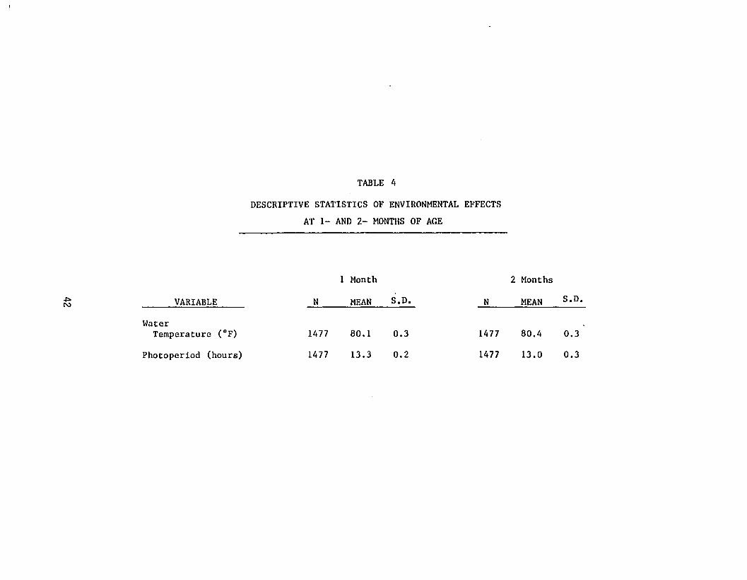
TABLE 4
DESCRIPTIVE STATISTICS OF ENVIRO~ffiNTAL EFFECTS
AT 1- AND 2- MONTHS OF AGE
1 Month 2 Months
~ VARIABLE N MEAN S.D. N MEAN S.D.N -
WaterTemperature (OF) 1477 80.1 0.3 1477 80.4 0.3
Photoperiod (hours) 1477 13.3 0.2 1477 13.0 0.3

TABLE 5
DESCRIPTIVE STATISTICS OF ENVIRO~ffiNTAL EFFECTS
AT 3- TO 5- MONTHS OF AGE
3 Months 4 Months 5 Months
VARIABLE N MEAN S.D. N MEAN S.D. N MEAN S.D.
MALES:
WaterTemperature (OF) 971 80.0 0.5 971 79.1 1.1 971 77 .4 1.4
.(:::0w
Photoperiod (hours) 971 12.5 0.3 971 11. 9 0.3 971 11.3 0.2
Density (fish/cage) 971 22.1 4.2 971 21.6 4.5 971 21.4 4.6
FE~1ALES:
WaterTemperature (OF) 733 80.0 0.5 733 79.1 1.1 733 77 .4 1.4
Photoperiod (hours) 733 12.5 0.3 733 11.9 0.3 733 11.3 0.2
Density (fish/cage) 733 22.2 4.2 733 21.8 4.5 733 21.7 4.5

expressed in the form of very high standard errors for the
estimated regression parameter. This indicates one of the
highly correlated independent variables should be dropped
from the analysis (Pindyck and Rubinfeld, 1981). Since
this experimental design is unbalanced with respect to
time, the correlations between environmental effects from
monthly family means are correpondingly low. Thus
collinearity is not a concern. When simulataneously
incorporated into the multiple regression model, the
regression coefficients of water temperature, photoperiod,
and density did not have unduly large standard errors
(Appendix 3a,b). There is no bias due to misspecification
of the model. Furthermore, a F-test of the additional sum
of squares from the simultaneous inclusion of temperature,
photoperiod, and density over that of a one or two
independent variable model proved to be a significantly
better regression model. The coefficient of determinat{on
of the three independent variables was approximately 15
percent.
All first order interaction effects were found not
to be significant. In addition, the effects of water
temperature, photoperiod, and density were judged to be
linear because their second degree terms in the regression
model were cal cul ated, tested, and found to be
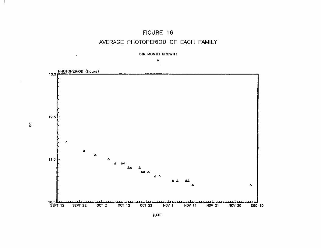
insignificant. This is illustrated by the average water
temperature graphs (Figures 7 to 11) and average
44

photoperiod graphs (Figures 12 to 16) for each family at
1- to 5- months of age. None of these graphs are
curvilinear. Although there were 61 families, less than
that number are shown because some families were born on
the same day and, thus, share the same average values.
Growth was adjusted to a water temperature of 80 degrees
Farenheit, a photoperiod of 12 hours of light per day, and
a density of 20 fish per cage.
The least squares adjustment factors for the
environmental effects of water temperature, photoperiod,
and density have been tabulated in Appendix 3a for 1- and
2- month old data and 3b for 3- to 5- month old data. It
is interesting to note that the significant regression
coefficients of water temperature, photoperiod, and
density in all traits in every month class have slopes
that are respectively positive, negative, and negative.
The positive slope of water temperature implies that
growth was promoted by increased water temperature ·for
increased metabolic activity. Lower cage density very
likely led to reduced conspecific interaction or
competition, hence, more growth. The negative growth
effect of lengthened photoperiod was possibly created by
oxygen depletion due to prolonged photosynthetic activity
of the various micro and macro algal communities growing
on the cages.
In addition to the effects of water temperature,
45

FIGURE 7
AVERAGE TEMPERATURE OF EACH FAMILY1st MONTH GROWTH
*
*** ******* *** * ******
TEMPERATURE (Farenhoft)81 ,_ - ,
79*
~ 78m
75
73 [' , , '~' , , , ' ....I.M' , , I l..u..l~L.u.l.J.1.1..J.M.u.I...lJ...u..L.L!.Jr~J...u.bY 4,,+1 I.J.! Y LL+6"*.LY.I,1.1MAY 15 MAY 25 JUNE 4 JUNE 14 JUNE 24 JULY 4 JULY 14 JULY 24 AUG 3 AUG 13
DATE
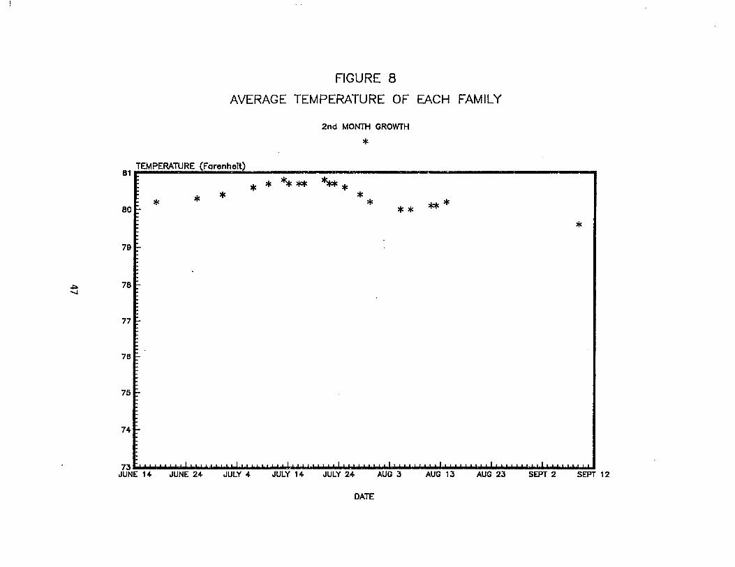
FIGURE 8
AVERAGE TEMPERATURE OF EACH FAMILY
2nd MONTH GROWTH
*TEMPERATURE (Forenhelt)
81 , ,
* * **** ****801-
79f~ 781-"'-J
nl
761-
751-
741-
* * * * * ** ****
73~ ' I I I , , , , I I I , , , , , , I ! I I , , 'M.a61mJ , , I , , , I I I , , , I , , I I I I , , I I I I I
JUNE 14 JUNE 24 JULY 4 JULY 14 JULY 24 AUG 3 AUG 13
DATE
....w.r..AUG 23
"I, ,
SEPT 2 SEPT 12

FIGURE 9
AVERAGE TEMPERATURE OF EACH FAMILY
3rd MONTH GROwrH
*TEMPERATURE (FarenheTt)
81 E ,
*
801-
791-
.j:>o 781-CO
77F-
761-
751-
741-
** * * **** **** ** ** ** *
*
L' , I I , I
JULY 24JJ.
AUG 3~,,1d J+.L'd
AUG 13~
AUG 23
DATE
~SEPT 2
! I I J I , I
SEPT 12w.J..&.i..I
SEPT 22.I.dJ..I..I.OCT 2
.OCT 12

FIGURE 10
AVERAGE TEMPERATURE OF EACH FAMILY
4th MONTH GROWTH
*TEMPERATURE (Farenhelt)
81' .,
~1.0
801-
F
79t
781-
* * ** *
******** ** ** **
*77r:-
761-
*751-
741-
NOV 11I , , I • .1.
NOV 1'" I I
OCT 22...u..L.u.
SEPT 2L' I I '4
AUG 23....
DATE

FIGURE 11
AVERAGE TEMPERATURE OF EACH FAMILY
5th MONTH GROWTH
*TEMPERATURE (Farenhelt)
81 Ii 'IW:Iol ·e. ,
Ulo
78
77
** * * * ****
*** * **
76 **
** *
74
*-'J..UDEC 10OCT 2SEPT 22
731dd I I I , , I I I I ! '=Y ' 1 , ',b&"J.J...LJ..L.L.J.4L.l~LLU!.bl.l,..L14.L,t,.L.LL1,,~~bJ.1 LIlli I 1 , I I , I 4" dadSEPT 12
DATE

FIGURE 12
AVERAGE PHOTOPERIOD OF EACH FAMILY
1st MONTH GROWTH
b.
PHOTOPERIOD (hours)13.5' ,
ent-'
12.51-
11.51-
b. b..6. b. b. MM b.Mb. b.b.
b.b.
Mil.
b.
""'" I, ,MAY 25
..l.1.l..IJUNE 4
'" I" """ I IJUNE 14 JUNE 24
DATE
~JULY 4
'" I"""", I"JULY 14 JULY 24
.....L.r..a.AUG 3 AUG 13

FIGURE 13
AVERAGE PHOTOPERIOD OF EACH FAMILY
2nd MONmH GROWTH
.6.
PHOTOPERIOD (hours)13.5. ,
.6.
.6.
A AA M
M MA A .6.
.6.
12.5 --
6.
6. 6.
.6.6.U1N
.6.
11.51-
SEPT 12.......
SEPT 2..w...
AUG 23..w...
AUG 13.w.
AUG 3'" I",JULY 24
w.rJ.JULY 14
~JULY 4
&"", ,. ,JUNE 24
10.5 ........JUNE 14
DATE

FIGURE 14
AVERAGE PHOTOPERIOD OF EACH FAMILY
3rd MONTH GROWTH
/).
PHOTOPERIOD (hours)
13.5l I/).
66
/).
/).
10.5 ........JULY 1...
<J1W
12.51-
11.51-
.... '""JULY 2...
......L..I..I.AUG 3
MM
iJ.w.AUG 13
A.A.6./). /).
/).
l.IJ.AUG 23
DATE
/)./).
~SEPT 2
/).
/)./).
""""'"SEPT 12IooIoJ.
SEPT 22"", ,OCT 2
6
OCT 12

(.J1
+::>
FIGURE 15
AVERAGE PHOTOPERIOD OF EACH FAMILY
4th MONTH GROWTH
I:.
PHOTOPERIOD (hours)1~5, ,
12.5~ I:.
ll.ll.
ll.ll.
J:J:J; M~
ll. ll.ll.
11.5 .... 1:.1:.
M ll.
ll.
10.5 .........AUG 13
",'," ,AUG 23
I"""" I I
SEPT 2 SEPT 12"I" ,
SEPT 22
DATE
"I" ,
OCT 2,,', ,
OCT 12,,',"""',', ,
OCT 22 NOV 1.
NOV 12
0101
FIGURE 16
AVERAGE PHOTOPERIOD OF EACH FAMILY
5th MONTH GROWTH
A
PHOTOPERIOD (hours)13.5n--- -- ---- ...
12.5
A
AA
11.5 AA AA
AA AAAA
AAAA AA
A A
10.5' , I I , I , , , , I I J, Y"&+' I I , , , , I 1 J I ld I" 1..J.1.1.1.J...1,J.l.L'. , , I , ld-l.L~L.l-.u..LL.&.1.+,L.J-,y,1 , I .4y.&J: ' , I,LLh'~SEPT 12 SEPT 22 OCT 2 OCT 12 OCT 22 NOV 1 NOV 11 NOV 21 NOV 30 DEC 10
DATE

photoperiod, and density there were probably other factors
involved in this study. For example, the influence of
micro-environmental differences from the location of cages
at the experimental site could not be estimated because of
the confounding of sires and dams with cage location. The
sex composition in a family was thought to have an
important social interaction effect, but when tested in
the statistical model was found to be insignificant. Other
factors influencing body measurements probably existed in
this study but remain unidentified.
GENETIC ANALYSIS
The mean squares for 1- and 2- month old traits
are shown in Table 6 after data were adjusted for water
temperature and photoperiod. Density was not considered.
Difference among dams within sires were highly significant
for all traits (p<O.Ol), but differences among sires were
not significant. For the 1- month old fish measurements,
the sire mean squares are smaller than the dam mean
squares suggesting a zero sire component of variance. This
is reflected in the variance components estimated in Table
7. In 2- month 01 d fi sh measurements a si re component was
recorded, but is not statistically significant. To follow
the change in the components of variance between 1- and 2
months of age, Table 8 shows the additive genetic,
56

TABLE 6
ANOVA OF TRAITS AT 1- AND 2- l-tONTHS OF AGE-
SOURCE df 1 Month 2 Months
WEIGHT:
Sire 30 5.52 134.05
Darn/Sire 30 6.58 ** 83.74 **Residual 1416 0.22 7.01
TOTAL LENGTH:
Sire 30 853.50 1760.01
Darn/Sire 30 890.88 ** 968.19 **Residual 1416 33.54 102.26
Ul HEAD:......Sire 30 55.47 100.18
Darn/Sire 30 59.31 ** 55.59 **Residual 1416 2.25 6.61
HEIGHT:
Sire 30 88.39 176.94
Darn/Sire 30 97.57 ** 103.17 **Residual 1416 3.88 11.13
*p < 0.05
**p < 0.01
K COEFFICIENTS
Kl = 22.06K2 = 26.28K3 = 47.56

TABLE 7
VARIANCE COMPONE~ITS FOR TRAITS
AT 1- AND 2- MONTHS OF AGE
VARIANCECOMPONENT WEIGHT LENGTH HEAD HEIGHT
1 Month:
(j~ 0.00 0.00 0.00 0.00
(f'Z. 0.29 38.87 2.59 4.251)
<r~ 0.22 33.54 2.25 3.88
2 Months:
(S''2.0.75 13.17 0.74 1.185
a' 3.48 39.26 2.22 4.171)
(j2 7.01 102.26 6.61 11.13'oJ
<S: = Sire Component
6~ = Dam Component
(f~= Within Progeny
58

TABLE 8
PERCENTAGE OF GENETIC, MATERNAL, ANn ENVIRONMENTAL VARIATION
RELATIVE TO PHENOTYPIC VARIATION AT 1- AND 2- MONTHS OF AGE
TOTALVARIANCE WEIGHT LENGTH HEAD HEIGHT
1 Month:
V(G) 0.0 0.0 0.0 0.0
V(M) 56.9 53.7 53.5 52.3
V(E) 43.1 46.3 46.5 47.7
2 Months:
V(G) 26.7 34.1 30.9 28.6
V(M) 24.3 16.9 15.5 18.1
V(E) 49.0 49.1 53.6 53.2
V(G) = Additive Genetic Variance
V(M) = Maternal Variance
V(E) Environmental Variance
59

maternal, and environmental components of variance as
percentages. The percentage of genetic variance exhibits a
marked increase with time while the maternal variance
percentage decreases. Although differences among sires
were not significant, the potential trend corresponds with
Kirpichnikov (1982) who states that early environmental
variation (e.g. maternal variation) is very high at early
stages of a fish's life, but decreases thereafter with a 2
to 3 times comcomitant increase in the heritability of
weight and size. Since differences among sires were not
significant, the heritabilities and genetic correlations
were not estimated.
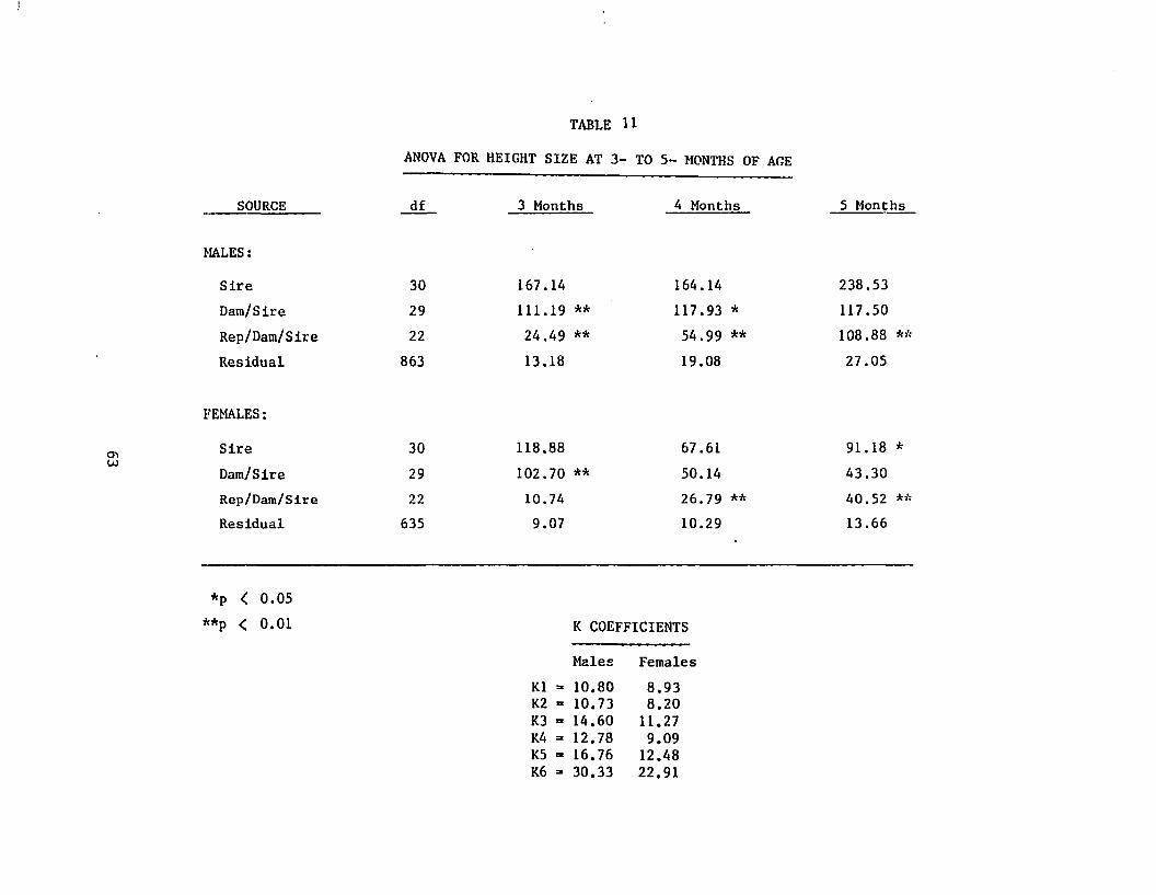
The ANOVA for weight at 3- to 5- .. months of age
after adjustment of data is shown in Table 9. The mean
square values for the males was notably higher than the
females thus justifying the separate analysis by sex. The
ANOVA table for weight is quite representative of the
other traits of total length, head, height, dr awnwe i qh t ,
intestinal length, and gill surface area (Tables 10 to
13). In general, the difference among dams within sires
were significant for all the traits through time, but
differences among sires were not significant. However,
where sire differences occurred, especially at the fifth
month, the differences among dams within sires were not
significant. There was no instance when both the among
sire and among dam within sire differences were
60

TABLE 9
ANOVA FOR HEIGHT AT 3- TO 5- MONTHS OF AGE .SOURCE df 3 Honths 4 Honths 5 Months
MALES:
Sire 30 568.58 1566.43 3247.73
Dam/Sire 29 357.64 ** 900.58 * 1789.86
Rep/Dam/Sire 22 65.35 ** 374.57 ** 1273.99 1,1,
Residual 863 32.41 108.22 247.72
FEMALES:
Sire 30 116.61 345.21 651.33 **en Dam/Sire 29 77 .80 ** 196.03 * 249.90I-'
Rep/Dam/Sire 22 16.80 94.18 ** 254.96 **Residual 635 15.89 37.07 73.02
*p .( 0.05
**p <: 0.01 K COEFFICIENTS
Males
Kl .. 10.80K2 .. 10.73K3 .. 14.60K4 .. 12.78K5 .. 16.76K6 .. 30.33
Females
8.938.20
1l.279.09
12.4822.91

TABLE 10
ANVOA FOR TOTAL LENGTH AT 3- TO 5- MONTHS OF AGE
SOURCE df 3 Months 4 Months 5 Months
MALES:
Sire 30 1884.37 2018.20 2393.67
Dam/Sire 29 1208.48 ** 1299.01 ** 1373.23
Rep/Dam/Sire 22 196.47 427.74 ** 804.73 **Residual 863 136.46 187.45 252.80
FEMALES:0'\N Sire 30 479.79 759.11 963.31 *
Dam/Sire 29 465.79 ** 504.18 * 410.85
Rep/Dam/Sire 22 103.93 232.65 ** 318.46 *,'{Residual 635 84.42 100.49 128.67
*p < 0.05
**p < 0.01 K COEFFICIENTS
Males
Kl :z 10.80K2 :z 10.73K3 :z 14.60K4 :z 12.78K5 :z 16.76K6 :zo30.33
Females
8.938.20
11.279.09
12.4822.91
*p < 0.05
**p < 0.01 K COEFFICIENTS
Males
Kl :z 10.80K2 :z 10.73K3 :z 14.60K4 :z 12.78K5 = 16.76K6 :z 30.33
Females
8.938.20
11.279.09
12.4822.91

TABLE 12
ANOVA FOR HEAD SIZE AT 3- TO 5- NONTHS OF AGE
SOURCE df 3 Months 4 Honths 5 Months
MALES:
Sire 30 106.29 112.78 150.05 '/(
Dam/Sire 29 67.39 )~* 70.63 ** 65.28
Rep/Dam/Sire 22 12.46 24.42 ,~* 49.65 *ic
Residual 863 8.36 12.45 16.54
FEMALES:
Sire 30 26.16 38.60 52.61 *0'1
Dam/Sire 25.87 ** 25.94~ 29 20.70
Rep/Dam/Sire 22 7.54 15.68 ** 18.33 *1(
Residual 635 5.20 5.71 7.65
*p < 0.05
>,c*p < 0.01 K COEFFICIENTS
Males Females
K1 ::0 10.80 8.93K2 ::0 10.73 8.20K3 ::0 14.60 11.27K4 ::0 12.78 9.09K5 ::0 16.76 12.48K6 ::0 30.33 22.91

TABLE 13
ANOVA FOR DRAWNlolEIGHT, INTESTINAL LENGTH, AND GILL SURFACE AREA
AT 5- MONTHS OF AGE
SOURCE df Drawnweight df Intestine df Gills
MALES:
Sire 30 2335.26 30 448324.00 * 30 151317.00 **Dam/Sire 29 1399.59 29 191067.00 28 45161.60
Rep/Dam/Sire 22 988.97 ** 22 152479.00 ** 20 55022.20 "0"
Residual 861 199.63 861 30597.70 , 835 8299.95
FEMALES:
Sire 30 466.16 * 30 164632.00 ** 30 36890.10
Dam/Sire 29 198.89 29 59123.00 28 18628.90 *Ol Rep/Dam/Sire 22 199.50 ,~* 22 42159.50 ** 20 9183.41 *~<U1
Residual 634 56.58 634 16335.30 613 3845.59
'~p < 0.05 K COEFFICIENTS K COEFFICENTS K COEFFICIENTS**p < 0.01 (DrawnweiRht) (Intestine) (Gills)
Males Females Males Females l~ales FemaLes
Kl = 10.78 8.90 10.78 8.90 10.95 8.84K2 .. 10.71 8.20 10.71 8.20 10.61 8.31K3 .. 14.58 11.27 14.58 11.27 14.30 11.19K4 .. 12.75 9.08 12.75 9.08 12.84 9.08K5 .. 16.72 12.45 16.72 12.45 16.50 12.11K6 .. 30.26 22.87 30.26 22.87 29.32 22.09

significant.
The repl ication differences demonstrated an
increasing level of significance from 3- to 5- months of
age in all observed traits. This source of variation
represented the contemporaneous effect between cages.
In Table 14, variance components were
re-calculated after partitioning out replicate effects
derived from the replicated family data. The mean squares
were then re-calculated accordingly with significant among
sire and among dam within sire differences observed in
both males and females at 4- months of age for weight and
in males only at 5- months of age for weight, drawnweight,
and total length. The estimated narrow-sense
heritabilities derived from the sire component of variance
for these traits are shown below:
MONTH
4 5
MALES
Weight 0.39 0.39
Drawnweight 0.31
Total Length 0.31
FEMALES
Weight 0.39
The genetic correlations for the above male traits
66

TABLE 14
VARIJL~CE COMPONENTS FOR TRAITS AT3- TO 5-MONTHS OF AGE
VARIANCE TOTAL DRAt-.'N-COMPONENT HEIGHT LENGTH HEAD HEIGHT tVEIGHT INTESTINE GILLS
MALES
3 Months:
o~ 5.37 17.06 1.00 1.37cr; 16.47 65.79 3.59 5.50
(f~ 38.98 145.47 R.91 14.65
4 Uonths:
()'~ 18.12 18.32 1.11 1.0502
29.60 57.21 2.97 4. J.2'D
(il 139.05 211. 92 13.74 22.56IN
5 Months:
~~ 40.67 28.25 2.56 3.56 24.92 7735.07 3389.51
6; 41.95 43.32 1.28 2.14 33.76 4510.59 104.74
(f"Z. 335.14 298.99 19.36 34.99 266.78 39979.31 11814.34w
FEMALES
3 Months:
u; 1. 41 0.00 O.CO 0.27
0; 5.7.2 31.68 1.56 7.97(jl 16.19 87.17 5.55 9.46
VI
4 Months:
<r; 5.78' 9.26 0.46 0.58
cr~ 7.77 24.11 1.10 2.10'(J2- 45.15 116.22 6.71 12.24IN
5 Months:
<5~ 16.73 22.83 1.33 1.96 11.08 4510.29 769.32(jz 4.09 11.89 0.50 1.01 3.35 103.11 716.51D
(j~ 90.17 147.61 8.64 16.10 70.29 20736.06 4610.51
a~ ='Sire Componentc:r; = Dam ComponentU;, = Within Progeny Component
67

DRAWN TOTALWEIGHT-5 WEIGHT-5 LENGTH-5
0.92 0.88 0.87
are as follows:
WEIGHT-4
WEIGHT-5
DRAWNWEIGHT-5
TOTAL LENGTH-5
WEIGHT-4
1.01 0.95
0.94
The larger variance components in males than in
females is a reflection of their sexually dimorphic growth
rate. The current explanations for the cause or mechanisms
of dimorphism in tilapia range from II i ncompl etel y
understood II to lI unknown . 1I Lowe-McConnell (1982) suggests
an environmental and behavioral basis of sexually
dimorphic growth rather than a genetic one. It is possible
that precocious sexual maturation in females for
vitellogenesis may stunt growth more than in males for
spermatogenesis) thus) providing smaller variance
component estimates in females than in males. The
variability in the onset of sexual maturity in males and
females have not been adequately studied in tilapia
(Jalabert and Zohar, 1982). However, if females mature
earlier than in males the switch from growth to
reproduction may also account for their smaller observed
variances.
For both sexes, the dam variance components in 3-
68
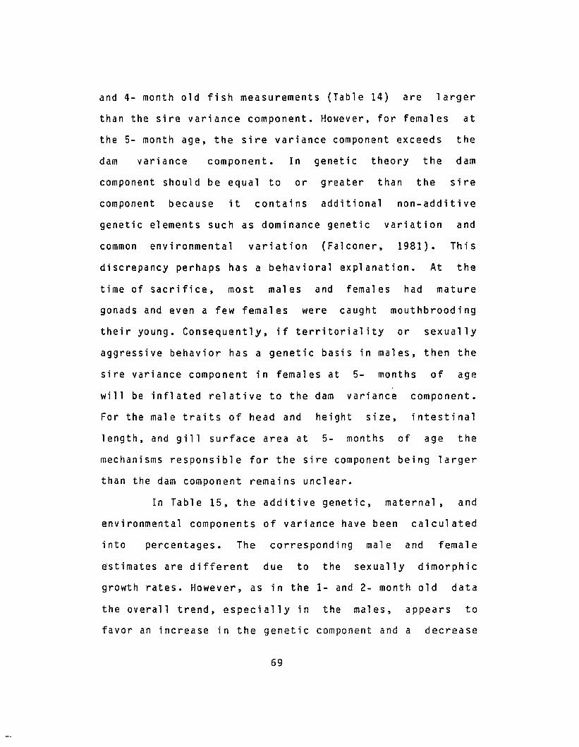
and 4- month old fish measurements (Table 14) are larger
than the sire variance component. However, for females at
the 5- month age, the sire variance component exceeds the
dam variance component. In genetic theory the dam
component should be equal to or greater than the sire
component because it contains additional non-additive
genetic elements such as dominance genetic variation and
common environmental variation (Falconer, 1981). This
discrepancy perhaps has a behavioral explanation. At the
time of sacrifice, most males and females had mature
gonads and even a few females were caught mouthbrooding
their young. Consequently, if territoriality or sexually
aggressive behavior has a genetic basis in males, then the
sire variance component in females at 5- months of age
will be inflated relative to the dam variance component.
For the male traits of head and height size, intestinal
length, and gill surface area at 5- months of age the
mechanisms responsible for the sire component being larger
than the dam component remains unclear.
In Table 15, the additive genetic, maternal, and
environmental components of variance have been calculated
into percentages. The corresponding male and female
~stimates are different due to the sexually dimorphic
growth rates. However, as in the 1- and 2- month old data
the overall trend, especially in the males, appears to
favor an increase in the genetic component and a decrease
69

TABLE 15
PERCENTAGE OF GENETIC, MATE~~AL, AND ENVIROm1ENTALVARIANCE Cm1PONENTS AT 3- TO 5-MONTHS OF AGE
VARIANCE TOTAL DRA~·lN-
COHPONENT w"EIGHT LENGTH HEAD HEIGHT HEIGHT INTESTIt\E GILLS
MALES
3 Months:
V(G) 35.3 29.9 29.6 25.5V(M) 18.3 21.3 19.2 19.2
VeE) 46.4 48.8 51.2 55.3
4 Months:
V(G) 313.8 2.'5.5 24.9 15.1
V(M) 6.1 13.5 10.4 11.1
VeE) 55.0 61.0 64.6 73.8
5 Months:
V(G) 39.2 30.5 41.8 35.5 30.6 55.8 72.9
V(M) 0.3 4.1 f! /,1 2.7 IF II.r
VeE) 60.5 65.4 58.2 64.5 66.7 44.2 27.1
FEMALES
3 Months:
V(G) 24.6 O. o 0.0 6.1
V(M) 16.7 26.7 21.9 43.5
VeE) 58.7 73.3 78.1 50.4
4 Months:
V(G) 39.4 24.8 22.2 15.5
V(M) 3.4 9.9 7.7 10.2
VeE) 57.2 65.3 70.0 74.3
5 Months:
V(G) 54.1 47.2 47.1 39.2 47.9 60.6 50.0
V(M) II II II f! f,f II II
VeE) 45.9 52.8 52.9 60.8 52.1 39.4 50.0
V(G) = Additive Genetic VarianceV(M) = Maternal VarianceVeE) = Environmental Variance
II indicates V(M) <. 0
70

; n the maternal component.
71

v. GENERAL DISCUSSION
Five founder specimens collected in Java in 1939
were responsible for the extant O. mossambicus populations
in the Asia/Pacific region. As a testimony to their
successful colonizing abilities, this fish has become an
established exotic able to exploit a wide spectrum of
aquatic environments in the tropical developing countries
of Asia and Oceania. In 1951, fourteen O. mossambicus
individuals were reported introduced into Hawaii from
Singapore. This study investigated the genetic variation
of economic traits in the Hawaiian O. mossambicus
population.
In spite of the potentially depauperate gene pool
in the above founder specimens and Malecha1s (1968) study
indicating serum esterase and transferrin loci were
monomorphic, the results from this study reveal the
presence of genetic variation in O. mossambicus.
Significant differences among sires and among dams within
sire were found in males and females for weight at 4
months of age and in males only at 5- months of age for
weight, drawnweight, and· total length. The estimated
heritabilities on these traits were found to lie in the
intermediate range with genetic correlations ranging from
0.87 to unity.
72

Allendorf and Utter (1979) hypothesized that the
amount of genetic variation by isozyme loci in fish is an
indicator of the genetic variation throughout the genome
of that population. Therefore, populations with a high or
low average heterozygosity should generally demonstrate
high or low additive genetic variation. However, in this
instance, it appears the two Hawaiian isozyme data
reported by Malecha does not reflect the amount of genetic
variation observed in this study. Unfortunately, no other
work in or outside of Hawaii on electrophoretic variation
within O. mossambicus populations has been done to compare
results. Since polygenic or quantitative traits are, by
definition, assumed to be" contro~led by many genes it is
unlikely that there is no genetic variation or that all
loci are fixed in the same direction in the population.
Thus estimation of genetic variation by isozyme
frequencies should be interpreted with caution, and is no
substitute for estimating the genetic variation or
heritabilities of economic traits.
The disparity between the findings of this study
and Malecha's results may be explained by studying a
summary of the reported tilapia introductions to Hawaiian
waters (Maciolek, 1984), as follows:
73

SPECIES SOURCE NUMBER IMPORTED YEAR
~eochromis mossambicus Sin~apore 14 1951+
O. maeroohi» Congo 52 1958+
Sarothe1'odOn meZanothe1'on ? ? )1970
TiZapia meZanopZeura Congo 50 1957
T. zUZU ~Iest Jndies 19 1957+
It is possible that in addition to genetic drift for
monomorphism the 1 locus, 2 allele systems in serum
esterase and transferrin were already fixed in the small
number of introduced O. mossambicus individuals. The
polymorphisms found in Q. macrochir and T. melanopleura
had an increased probability of detection when noting that
52 and 50 specimens were introduced respectively. Genetic
variation in Q. mossambicus may also have increased since
1951 from mutations, hybridizations with other tilapia
species, or through subsequent unreported introductions of
O. mossambicus into Hawa t t .
The amount of genetic variability reported in this
study is not surprising. Although Q. mossambicus in Hawaii
has undergone two founder events this does not necessarily
lead to greatly reduced levels of variability. For
example, Ne i , Maruyama, and Chakroborty (1975) and
Templeton (1980) have respectively studied this topic by
computer simulation and empirical investigations. They
demonstrated that if a polygenic trait is controlled by a
74

large number of loci each having small additive effects,
then there is often very little change in genetic
variability after the founder effect. It appears that if
the founder genome is sufficiently heterozygous it can
survive and genetically respond to the forces of drift and
altered selective forces provided there is an open niche
to allow a population flush. A clear example of such a
case is provided by Carson's (1978) comprehensive studies
documenting the repeated inter-island founder events by
the Hawaiian Drosophila.
METHODOLOGICAL CONSIDERATIONS
One of the major problems in the methodology of
experiments in animal genetics is synchronous mating or
spawning dates in families. The reason for such concern is
that fishes, as opposed to mammals, are known to be more
sensitive to environmental variations, e.g. water
temperature, density, competition, food availability, and
water quality (Gall and Gross, 1978a; El-Ibiary and Joyce,
1978). Hence, uniformity of environmental conditions is
particularly important when evaluating quantitative
traits.
This problem of asynchronous mating of sires and
dams has been overcome through artificial fertilization
techniques. These are regularly practiced in salmonids.
75

the
been
overadvantages
variance in
design has
Stripping of gametes and artificial fertilization have
already been demonstrated in tilapia (Rothbard and
Prugenin, 1975). In conjunction, a successful egg
incubation system has been devised (Rothbard and Hulata,
1975). However, these techniques have never been attempted
on a large scale. If artificial fertilization were
practiced in this study, the time effects of water
temperature and photoperiod would have been eliminated.
Other studies could likewise have benefited from
artificial fertilization, but instead have encountered
difficulties using "na t ur a l service." For example, in
channel catfish, Reagan et ale (1970) produced inflated
heritability estimates for weight and length traits
because of assortative mating. Female breeders had to be
of equal or smaller size than the males to prevent injury.
Artificial fertilization paves the way for a more
precise approach to estimating genetic variation in
tilapia by analysis of variance techniques. The ideal
experimental design would be a factoral design whereby all
sires and dams would be simultaneously mated to each
other. The lack of incubation units for fertilized eggs
prevented the implementation of a factoral experiment for
this study.
The factoral design has distinct
the hierachal design. A lower error
heritability estimates using a factoral
76

demonstrated using real data with the long head poppy
(Papaver dUbium) (Kearsey, 1965) as well as with simulated
data (Pederson, 1972). The simulation study of Pederson's
suggests the required number of sires in a factoral design
would be less than that required in a hierarchical design
in order to get the same amount of genetic information.
This is an important consideration since the number of
testable sires is almost always governed by the
capabilities of the testing facility.
Refstie and Steine (1978) used a hierarchical
design to estimate heritabilities for weight and length of
freshwater Atlantic salmon using 62 sires and 33,000
observations of offspring. They cite Henry (1968) in
estimating that the same level of accuracy in their study
would be obtained with only 3000 observations of offspring
if sire numbers were increased from 62 to 100. However,
the testing of 100 sires is a very demanding study. The
advantage in the factoral design of requiring fewer sires
to get the same amount of genetic information is much
appreciated by any investigator.
In addition, the factoral design is superior to
the hierarchical design in partitioning components of
variance (Becker, 1975). Maternal variation in tilapia can"
be partitioned without the confounding effects of
dominance genetic variation. The interaction of genotypes
or sire x dam interaction can also be partitioned, whereas
77

this effect is confounded in the dam variance component in
the hierarchical design.
PRACTICAL APPLICATION OF RESULTS
Tilapia culture is currently considered to have
significant impact in food programs for alleviating
protein shortages in developing tropical countries. Its
importance is undisputable. However, there appears a
difference of opinion among scientists on how to best
improve growth rate for increased production. For example,
Lowe-McConnell (1982) believes genetic factors are
unimportant relative to the manipulation of environmental
and behavioral mechanisms. In contrast, Gall (1983)
generally supports a genetic approach in fishes because
selection experiments on other fish species have resulted
in genetic responses typical of animal studies. A review
by Gjedrem (1983) showed that in 18 mass selection
experiments in a variety of fishes, 15 of those studies
showed positive genetic gains.
This study has revealed that growth in
o. mossambicus is not depauperate of genetic variation,
but has the potential to be improved by means of genetic
manipulation. The heritability estimates for weight and
total lengths were found to range between 0.31 to 0.39.
The Russian study by Chan (1971) had similar realized
78

heritability estimates for weight that ranged from 0.12 to
0.32.
It is of interest to note that the Asian
o. mossambicus which is in Hawaii is morphologically
different from the African O. mossambicus. The former is
long and cylindrical in contrast to the latter being
deep-bodied and generally growing to a larger size
(Pullin, 1982). Therefore, if growth rates in Hawaiian
Q. mossambicus are to be improved through selection, the
introduction of O. mossambicus from Africa should be
considered to increase the gene pool for optimal genetic
gains.
79

VI. APPENDIX 1
MEASUREMENT OF FISH LENGTHS USING A COMPUTER DIGITIZER
ABSTRACT
The use of a computer digitizer as a new technique
for measuring fish lengths was statistically compared
against the traditional method of measurement by a hand
ruler. Three judges measured four types of body lengths in
Oreochromis mossambicus. Each fish was measured by each
judge, three times by the digitizer method, and three more
times by the hand method. A two-way analysis of variance
revealed very strong (judge x method) interaction. When
the two methods of measurement were analyzed independently
of each other, their respective components of judge
variation were about equal. Thus the digitizer appears to
be a comparable new fish measuring tool that is equally
applicable to other aquatic species. This study also lists
its advantages and possible conditions which may affect
its measurement precision.
INTRODUCTION
classification, or taxonomic purposes
Fish measurements for growth
have
rate, age
traditionally
80
been done by the use of a reliable ruler. More recently.
still photography has captured the imagination of
scientists in improving new measurement techniques. For
example. juvenile salmon were photographed against a graph
paper background for estimation of their lengths (Martin.
1967) and weights of live fish have been estimated by
length and width measurements of their photographic images
(Hawkes. 1975; Christensen. Fiandt, and Benoit, 1977).
In the continuing improvement of length measuring
devices, the potential of the computer digitizer has yet
to be fully exploited. To demonstrate its usefulness, Frie
(1982) has measured fish scales and back calculated body
length using a digitizer coupled to an Apple II
microcomputer. However, the degree of reliability and
efficiency in this novel method relative to the hand
measurement is unknown. This study evaluates the two
methods by the comparison of their respective variance
components.
METHODS AND MATERIALS
A total of 24 live, unanaesthetized Cichlid fish
(Oreochromis mossambicus) were used as subjects with half
of them categorized as "small (juvenile)" (total length
40-70mm) and the other half as "large (adults)" (total
length 130-185mm). For each method of measurement. three
81

judges separately measured the total length, standard
length, height, and head size of the same fish. These
measurements were performed on each fish three times by
each judge.
HAND MEASUREMENT
The live fish subjects were placed into separate
water-filled glass containers that were labeled for
identification. Each of three judges randomly chose and
measured each fish by hand ruler at three different times.
The fish were returned to their individual containers
after each measurement.
DIGITIZER MEASUREMENT
Each fish was individually photographed in a
lateral position three separate times. A ruler was
included in each photograph's background to later
standardize measurements. Kodak ektachrome slide film was
used in a hand held single lens reflex camera equipped
with a macro lens. A single tensor lamp provided the light
source.
A computer program written in BASIC permitted
digitizing of a fish by placing the developed slide on the
lighted platen of a Hewlett-Packard 9874A digitizer
coupled to a Hewlett-Packard 2649G intelligent graphics
terminal. The logic for determining fish lengths was the
82

Pythagorean theorem in calculating the distance between
two points on the digitizer's platen grid. To improve the
measurement of fish details from a 35mm slide, binocular
magnifying glasses ("optivisor") were worn around the
forehead. To standardize body measurements in millimeters,
it was necessary to scale the fish using the ruler in the
photographic background. All data were stored on cassette
tape and later read into a Hewlett-Packard 3000 for
analysis.
STATISTICAL ANALYSIS
A two-way ANOVA with interaction was performed on
the following statistical model:
Yijk = mean + Ji + Mj + JiMj + R(error)ijk
where:
Yijk = the kth observation in the ith Judge and jth Method
mean = parametric mean of the population
Ji = random contribution of the ith Judge group
Mj = random contribution of the jth Method group
JiMj = interaction between the ith Judge and jth Method
groups
R(error)ijk = error term of the ith Judge and jth Method
83

A set of one-way ANOVAs on the methods of
measurement estimated the method effects of each judge
independent of the other two judges. The statistical model
for each judge was:
Yij = mean + Mi + R(error)ij
where:
Yij = the jth observation in the ith Method
mean = parametric mean of the population
Mi = random contribution of the ith Method
R(error)ij = error term of the jth item in the ith Method
A hierarchical ANOVA to estimate the variance
components of judg~ variation in fish groups were
separately analyzed for each method of measurement. The
analysis was performed on the following fish sizes: (1)
small fish only, (2) large fish only,and (3) all fish
pooled. The statistical model was:
Yijk = mean + Fi + Jij + eijk
where:
Yijk = the kth observation in the jth Judge subgroup of
the ith Fish group
mean = parametric mean of the population
84

Fi = random contribution of the ith Fish group
Jij = random contribution of the jth Judge subgroup in the
ith Fish group
eijk = error term of the kth observation in the jth Judge
subgroup in the ith Fish group
RESULTS
The F-values of the two-way ANOVA with interaction
indicated that not only are there highly significant
differences (p<O.01) in both main effects of judge and
method, but also highly significant is the (judge x
method) interaction. These results were consistent in all
four body measurements. This indicates that the effects of
the two factors were not simply additive.
To investigate the cause of the significant
interaction component, a least squares approach to
estimate method effects of each separate judge indicated
that the hand method generally gave smaller values in the
four body lengths compared to the digitizer measurements
(Table 16). The magnitude rather than the direction of
each judge's measurement appears to be the contributor to
the observed interaction component.
A clear interpretation of the two methods tested
was complicated by the presence of interaction. Therefore,
each method was separately analyzed by a hierarchal ANJVA
85

TABLE 16
LEAST-SQUARES MEANS AND STANDARD ERRORS OF METHODOF MEASUREMENT FOR FIXED EFFECTS OF FOUR VARIABLES
FOR EACH JUDGE
TOTAL STA.~DARD
LENGTH LENGTH HEIGHT HEAD
JUDGE 1
Overall Mean 108.19 87.00 33.39 28.00
Hand -0.82+.13 -1. 98+0.18 0.08+0.06 -0.95+0.11
Digitizer 0.82+.13 1. 98+0.18 -0.08+0.06 0.95+0.11
JUDGE 2
Overall Hean 107.72 85.92 32.68 28.33
Hand -0.93+0.10 -1. 38+0.15 -0.30+0.04 -0.45+0.07
Digitizer 0.93+0.10 1. 38+0.15 0.30+0.04 0.45+0.07
JUDGE 3
Overall Mean 107.91 86.27 32.55 28.36
Hand 0.06+0.09 -0.63+0.13 -0.40+0.06 -0.09+0.07
Digitizer -0.06+0.09 0.63+0.13 0.40+0.06 0.09+0.07
86

on a between judge within fish size basis to compare their
respective components of judge variation. From Table 17,
the digitizer method relative to the hand method generally
has a smaller pattern of variation. However, there are
several exceptions which merit explanation. An example is
when a judge measures the same fish three separate times,
the digitizer has a large within component of judge
variation in total length. In examining the replicate
photographic slides of each fish subject, it was founo
that the fish tail was sometimes tilted in the upward
direction in a replicate slide due to dorsal muscle
contraction at the region of the caudal peduncle. This
contributed to the increased variation which is less
noticeable in the small size fish. Increased variation due
to the tilted position of the tail is corroborated by the
consistently smaller variation in digitizer measurements
of standard length values which do not include the tail
length.
The digitizer method also has a larger within
component of judge variation in head size, which measures
the front of the snout to the outermost edge of the
operculum. This was caused by poor photographic lighting.
It was difficult to clearly define the operculum edge from
a slide image. This was particularly evident in the large
O. mossambicus where melanin pigments obscured visual
perception by turning the body a dark coloration when the
87

TABLE 17
THE BETt·lEEN AND WITHIN COMPONENTS OF VARIATION FOR JUDGES
W I T H I N B E T W E E N
H&~D DIGITIZER HAND DIGITIZERMETHOD METHOD METHOD METHOD
ALL FISH
Total Length 0.68 1. 33 1.27 0.24
Standard Length 0.78 0.73 3.30 3.25
Height Size 0.32 0.29 0.80 0.02
Head Size 0.44 0.57 0.92 0.00
SMALL FISH
Total Length 0.24 0.27 1. 31 0.06
Standard Length 0.21 0.17 2.86 0.15
Height Size 0.11 0.10 o.i i 0.03
Head Size 0.19 0.21 0.05 0.06
LARGE FISH
Total Length loll 2:40 1.22 0.42
Standard Length 1.36 1.29 3.74 6.36
Height Size 0.54 0.49 1.50 0.16
Head Size 0.69 0.93 1.80 0.00
88

fish was out of the water. In the small or juvenile sized
fish subjects, the melanin was not fully developed. Hence,
this problem was not as evident as shown by the almost
equal within component of judge variation in the hand and
digitizer methods.
In general, the digitizer method maintained a
smaller between component of judge variation than the hand
measurement. The difference in the between component of
judge variation in head size of small fish by the
digitizer (0.06) compared to the hand method (0.05) is
slight and considered negligible. However, standard length
in large fish has a significantly larger between component
of judge variation using the digitizer. This is possibly
attributable to the differing subjective judgements of
each judge in determining the photographic location of the
caudal peduncle. The lesser variation in the hand
measurement reveals each judge is better able to
repeatedly locate the caudal peduncle by feel rather than
sight. In contrast, the reverse is true in small fish
where the caudal peduncle is more difficult to find by
feel than by sight. These results may be interpreted as:
when one person always performs the measurement of
standard lengths in large fish, then the digitizer is a
more reliable method of measurement compared to the hand
method.
89

component of
the digitizer
as previously
DISCUSSION
This study statistically evaluated the differences
between a novel method of measuring fish lengths using a
computer digitizer against the traditional method of
measurement using a hand ruler. Four types of body length
measurements were used to test for differences between the
digitizer and hand methods. Analysis of variance revealed
very strong (judge x method) interaction throughout the
results. ConseG~ently, each method was analyzed on a
separate basis and then had their respective components of
judge variation compared.
In general, all the components of judge variation
were smaller with the digitizer than by hand. Exceptions
from this pattern were noted. First, the larger within
component of judge variation in head size could be
explained by poor lighting. This can be easily remedied by
improving the lighting source during the photographic
sessions. Second, the larger within component of judge
variation in the total length of large fish is caused by
tilting of the tail at the region of the caudal peduncle.
This problem can be minimized by relaxing the fish through
anaesthetizatlon.
The standard length's large between
judge variation found in large fish by
cannot be significantly reduced. However,
90

noted, the digitizer's within-judge component is smaller
than the hand method and is deemed the more reliable
method when one person consistently measures the standard
length in large fish.
In summary, these two methods of measurement
appear to be about equal. Although the components of judge
variation in the digitizer usually had smaller variances,
this study did reveal possible conditions which can
increase variation (e.g. fish body color, fish size, and
fish position during photography).
An investigator must take careful consideration of
the advantages a digitizer offers over the hand method of
measurement. In very small or delicate fish, the process
of photography for digitizing minimizes the handling
stress inherent in hand measurements. More important, each
fish retains a permanent record on film for calculation or
re-calculation of data at any time convenient to the
investigator. This property of a permanent record is an
asset generally unavailable in fish growth studies.
Lastly, since the digitizer directly records data to
memory devices, the tedium, time, and error of manual data
entry is notably reduced. The disadvantages of the
digitizing method in this study can be its monetary costs
(i.e. photography and digitizer/computer system) as well
as time and expertise required for film development
done by the investigator.
91
".1 I

The digitizer method is a comparable performer to
hand measurements and has potential applications not yet
fully exploited in the fishery sciences. This technique is
not limited to fish but can also be used on other aquatic
species for morphometric measurements in taxonomy as well
as for growth rate/size measurements in research and
management. Not only can linear size data be collected
from photographic slides, negatives, video tape
projections, or even x-rays, but the digitizer can also
map the coordinates of non-linear items, measure surface
areas, and reproduce precise drawings and outlines. The
broad and flexible scope of the digitizer can be a very
useful device on many subjects requiring quantification.
ACKNOWLEGEMENTS
This study was supported by the Hawaii Institute
of Marine Biology, Kaneohe, Hawaii, the Pacific Islands
Development Program, East West Center, Honolulu, Hawaii,
and the Data Computations Unit, Cancer Center of Hawaii,
Honolulu, Hawaii.
92

APPENDIX 2
DESCRIPTION OF BREEDERS AND BROODSHIPS
SIRE FARM 1 DAM FARM BIRT~ REP. CAGEDENSITy4NO. ORIGIN NO. ORIGIN l DATE NO. LOCATIO~~3
1 16 241 H 139
- - -1 P
1 42 2554 p ] R7
- - -J. 61 24
2 P 147- - -
2 L1 71 7
32 L 168- - -1 74 25
3 L 152- - -
3 H1 35 18
21 P 164- - -1 75 15
4 S 152- - -
4 P1 6 25
60 H 196- - -1 77 22
5 L 152- - --I 48 25
5 H 62 L 2222 16 23
1 64 063 L 179 I
- - -
93

APPENDIX 2 (Continued)
SIRE FAlU-! DAH FARM BIR~ REP. CAGEDENSITy4
NO. ORIGIN 1 NO. ORIGIN 1 DATE NO. LOCATION3
1 66 256 H 152
2 67 256 L
1 60 2411 P 147
2 43 25
1 38 197 H 152
2 28 157 L
1 69 248 P 152
2 28 24
1 37 179 L 152 .
- - -8 P
1 64 2558 ? 181
- - -1 27 25
10 H 152- - -
9 S1 32 4
35 S 176- - -1 31 21
12 L 152t - - -
10 H1 - 0
26 S 167I - - -
1 24 2513 L 158
2 55 2511 P
I1 I 12 25
38 S
I172
i 2 76 25
94
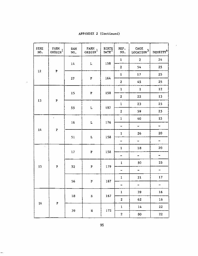
APPENDIX 2 (Continued)
SIRE FARM DAM FAlU-1 BIRT~ REP. CAGENO. ORIGIN 1
NO. ORIGINI DATE NO. LOCATION3 DENSITY4
1 2 2414 L 158
2 54 2512 P
1 17 2527 P 164
2 45 25
1 1 1215 P 158
2 22 1313 P
I 1 23 25II
55 L 1872 59 25
1 40 1516 L 176
- - -14 P
1 26 2051 L 158
I - - -
I 1 18 2017 P 158
- - -1 50 25
15 P 52 P 179- - -
1 21 1756 P 187
- - -1 39 16
18 S 1672 62 16
16 P1 14 22
39
IH 172
I2 SO 22
95

APPENDIX 2 (Continued)
SIRE "'ARM DAH FAR11 1 BIRT~ REP. CAGE ,~O. ORIGIN1
NO. ORIGIN DATE NO. LOCATION"" DENSITY l
1 57 2519 L 158
- - -17 P
1 41 1828 P 164
- - -1 63 25
20 L 161- - -
18 P1 19 25
61 L 2222 2 21
1 25 2419 H 22 P 167
- - -1 5 15
23 L 161- - -
20 L1 56 8
49 L 174- - -
1 3 1424 p 164
2 47 1421 H
1 51 1725 L 161
2 58 17
1 72 2229 L 168
- - -22 L
1 65 2557 H 189
- - -
96

APPENDIX 2 (Continued)
SIRE FARM nA.'t FARH BIRTZ REP. CAGENO. ORIGIN I
NO. ORIGINI DATE NO. LOCATION3 DENSITY 4
1 73 2523 L 30 H 172
- - -1 70 22
31 P 168- - -
24 L1 79 25
43 H 176- - -1 20 19
33 Ii 1652 78 19
25 p
1 11 1142 L 172
2 58 14
1 51 1234 L 194
- - -26 L I
I 1 49 25II 40 S 176
: - - -
I 1 9 2536 H 173
2 16 2527 II
1 13 2037 L 172
2 46 22,
1 10 2541 p 174
- - -28 P
,!
I 1 4 1545 L 174
II - - - I97

APPENDIX 2 (Continued)
SIRE °FARL'1 DAM FAIU'1 BIRT~ REP. CAGEDENSITY4NO. ORIGIN1
NO. ORIGIN1 DATE NO. LOCATION3
1 33 1346 H 193
2 52 1329 L
1 7 2253 L 187
2 30 9
1 8 1747 p 173
- - -30 H
1 15 2548 p 173
- - -1 53 15
50 L 174- - -
31 P1 44 24
I 59 P 196
I - - -
1Farms:H = Hanohano EnterprisesP = Seafood PlantationL = ArnorientS = Kahuku Prawn Co.
2Julian Calendar date.
3See Figure 1 for reference map of cage locations.
4Total number of fish per cage at 5 months of age.
98

APPENDIX 3a
ML~TIPLE REGRESSION COEFFICIENTS AND STANDARD ERRORSOF ENVIRONMENTAL EFFECTS AT 1 AND 2 MONTHS OF AGE
W E I G H T
TEMPERATURE PHOTOPERIOD
MONTH
1 0.15+0.08 -2.01+1.47
2 2.78+0.63 -4.92+0.56
TOT A L LEN G T H
TEMPERATURE PHOTOPERIOD
MONTH
1 L52+O.92 -23.64+1. 79
2 13.62+2.36 -18.31+2.09
H E A D S I Z E
TEMPERATURE PHOTOPERIOD
MONTH
1 0.32+0.24 -6.18+0.46
2 3.18+0.60 -4.28+0.53
H E I G H T S I Z E
TEMPERATURE PHOTOPERIOD
MONTH
1 0.40+0.31 -7.88+0.60
2 5.04+0.78 -6.35+0.69
99

· .
APPENDIX 3b
~ruLTIPLE REGRESSION COEFFICIE~ITS AND STA~DARD ERRORSOF ENVIRONHENTAL EFFECTS AT 3- TO 5-MONTHS OF AGE
MONTH
Males:
3
4
5
Females:
3
4
5
TEMPERATURE
0.55+1.46
10.13+1. 66
8.01+1. 54
2.25+1. 15
5.73+1.16
5.78+1. 01
WEI G H T
PHOTOPERIOD
-6.21+1. 76
-33.43+5.51
-25.43+9.79
-6.98+1. 33
-17.00+3.55
-:H. 18+5. 79
DENSITY
-0.48+0.07
-0.72+0.13
-0.66+0.20
-0.50+0.05
-0.45+0.08
-0.42+0.10
TEMPERATUREMONTH
Males:
3
4
5
Females:
3
4
5
5.03+2.91
14.57+2.12
8.36+1. 49
7.65+2.62
10.97+1. 89
7.86+1. 32
T 0 ~ ALL ENG T H
PHOTOPERIOD
-16.12+3.50
-48.00+7.04
-30.11+9.48
-18.92+3.10
-35.16+5.81
-29.68+7.55
100
DENSITY
-0.84+0.14
-0.86+0.16
-0.54+0.19
-0.98+0.12
-0.78+0.12
-0.63+0.14

APPENDIX 3b(Continued)
H E A D S I Z E
HONTH TEHPERATURE PHOTOPERIOD "DENSITY
Males:
3 1. 77+0. 71 -4.77+0.86 -0.16+0.03
4 3.67+0.53 -12.24+1. 78 -0.16+0.04
5 2.23+0.37 -6.68+2.37 -0.10+0.05
Females:
3 2.29+0.66 -5.29+0.76 -0.19+0.03
4 2.65+0.45 -8.78+1. 38 -0.16+0.03
5 2.07+0.32 -7.10+1.82 -0.14+0.03
H E I G H T S I Z E
MONTH TE~!PERATURE PHOTOPERIOD DENSITY
Males:
3 2.00+0.90 -5.04+1. 09 -0.28+0.04
4 3.75+0.67 -11.92+2.24 -0.23+0.05
5 2.28+0.48 -6.49+3.08 -0.15+0.06
Females:
3 2.66+0.89 -5.64+1.03 -0.33+0.04
4 3.16+0.61 -9.22+1. 86 -0.20+0.04
5 2.45+0.43 -9.20+2.47 -0.18+0.04
101

APPENDIX 3b(Continued)
DRAWNtfflIGHT AT 5 MONTHS
TEMPERATURE PHOTOPERIOD DENSITY
Males 6.99+1. 38 -24.02+8.75 -0.66+0.18
Females 4.85+0.89 -18.43+5.11 -0.39+0.09
INTESTINAL LENGTH AT 5 MONTIiS
TEMPERATURE PHOTOPERIOD DENSITY
Males 53.16+16.87 107.55+107.35 1. 29+2.15
Females 53.44+15.04 -40. fi7± 85.82 -0.40+1.55
GILL SURFACE AREA AT 5 MONTHS
TEMPERATURE PP.OTI)P~RIOD DENSITY
Nales 19.59+11. 61 91. 57+73. 39 1.84+1.42
Females 58.59+9.83 -169.68+56.17 0.33+0.99
102

VII. REFERENCES
Allendorf, F.W. and F.M. Utter. 1979. Population genetics.In: Fish physiology: bioenergetics and growth. Hoar, W.S.and D.J. Randall (eds.). Academic Press, New York. p.407-454.
Atz, J.W. 1954. The pereginating tilapia.57:148-155.
Anim. King.
Avtalion, R., Y. Prugenin, and S. Rothbard. 1975Determination of xenogenic markers in the genus ofTilapia. I. Identification of sex and hybrids in Tilapiaby electrophoretic analysis of serum proteins. Bamidgeh27:8-13.
Avtalion, R. and D. Mires. 1976. Determination ofallogeneic and xenogeneic markers in the genus of Tilapia.III. Electrophoretic identification of pseudohermaphrodlsmin I. aurea serum. Aquaculture 7:391-394.
Avtalion, R., M. Duczmines, A. Wojdani, and Y. Prugenin.1976. Determination of allogeneic and xenogeneic markersin the genus Tilapia. II. Identification of T. aurea, T.vulcani, and T. nilotica by electrophoretTc analysis oftheir serum proteins. Aquaculture 7:255-265.'
Avtalion, R.R. and 1.5. Hammerman. 1978. Sex determinationin Sarotherodon (Tilapia). I. Introduction to a theory ofautosomal influence. Bamidgeh 30:110-115.
toof
1979. Tilapia: A guidein Africa. University
Balarin, J.D. and J.P. Hatton.their biology and cultureStirling, Scotland. 174 pp.
Bardach, J.E., J.H. Ryther, and W.O. McLarney. 1972.Aquaculture: The farming and husbandry of freshwater andmarine organisms.
Basasibwaki, P. 1975. Comparative electrophoretic patternsof LDH and MDH in five Lake Victoria Cichlid species. Afr.J. Trop. Hydrobiol. Fish. 4:21-26.
Becker, W.A. 1975. ManualWashington State University170 pp.
of quantitative genetics.Press, Pullman, Washington.
Bondari, K., R.A.S. Castillo.for body weighton Tilapia in
Dunham, R.O. Smitherman, J.A. Joyce, and1983. Response to bidirectional selectionin blue tilapia. International SymposiumAquaculture, 8-13 May 1983, Nazareth,
103

Israel. (in press)
Borgstrom, G. 1978. The contribution of freshwater fishesto human food. In: Ecology of freshwater fish production.Gerking, S.D. (ed.). Blackwell Scientific Publications,Oxford. p. 469-491.
Brock, V.E. 1954. A note on the spawning of Tilapiamossambica in seawater. Copeia 1954(1):72.
Carson, H.L. 1978. Speciation and sexual selection inHawaiian Drosophila. In: Ecological genetics: Theinterface. Brussard, P.F. (ed.). Springer-Verlag, NewYork. p, 93-107.
Chan, May-Tchien. 1971. Experience with the determinationof realized weight heritability in the tilapia (Tilapiamossambica Genetika (Moscow) 7(1):53-59(RE).
Chen, F.Y. 1969. Preliminary studies on the sexdetermining mechanism of Tilapia mossambica Peters and T.hornorum Trewavas. Vehr. Int. Ver. Limnol. 17:719-724.
Chen, F.Y. 1983. Inheritance of biochemical markers of S.mossambicus and S. hornorum in F2 and backcross hybrids,and its potentTal in filapia culture. InternationalSymposium on Tilapia in Aquaculture, 8-13 May 1983,Nazareth, Israel. (in press)
Chen, F.Y. and H. Tsuyuki. 1970. Zone electrophoreticstudies on the proteins of Tilapia mossambica and T.hornorum and their Fl hybrids, T. zi1lii and T.melanopleura. J." Fish. Res. Bd. Can.-27:2167-2177.
Chen, T.P. 1976. Aquaculture practice in Taiwan. FishingNews Books, Lt d , , Farnham, Surrey, England. 176 pp,
Christensen, G.M., J.T.Estimation of live fishFish-Cult. 39:41-42.
Fiandt, and D.A. Benoit. 1977.weight by photography. Progr.
Coche, A.G. 1982. Cage culture of tilapias. In: Thebiology and culture of tilapias. Pullin, R.S.V. and R.H.Lowe-McConnell (eds.). ICLARM Conference Proceedings 7,Manila, Philippines. 432 pp.
Davis, R.E., F.S. Foote, J.M. Anderson, and E.M. Mikhail.1981. Surveying theory and practice. McGraw-Hill BookCo., New York. p. 345-346.
Devambez, L.C. 1964. Tilapia in the South Pacific. SouthPacific Bulletin 14(4):27-28,52.
104

El-Ibiarys H.M. and J.A. Joyce. 1978. Heritability andbody size traits s dressing weight and lipid content inchannel catfish. J. Anim. Sci. 47(1):82-88.
Falconer, O.S. 1981. Introduction to quantitativegenetics. Longman, Inc , , New York. 340 pp •
FAO. 1980. Report of the ad hoc consultation on aquacultureresearch. FAa Fish. Rep. 238. 26 pp.
FAO. 1983. 1981 Yearbook of fishery statistics. Volume 52.U.N. Food and Agriculture Organization, Rome, Italy.
andpad
fish scalesa digitizing
Frie, R.V. 1982. Measurement ofback-calculation of body lengths usingand microcomputer. Fisheries 7(6):5-8.
Fryer, G. and ToO. Iles. 1972. The Gichlid fishes of theGreat Lakes of Africa. Oliver and Boyd, Edinburgh. 641pp.
Gall s G.A.E. 1983. Genetics of fish: A summary ofdiscussion. Aquaculture 33:383-394.
Gall, G.A.E.growth in13:225-234.
and S.J. Gross. 1978a. Genetic studies ofdomesticated rainbow trout. Aquaculture
Galls G.A.E. and S.J. Gross. 1978b. A genetic analysis ofthe performance of three rainbow trout broodstocks.Aquaculture 15:113-127.
Gates, G.E. and G-J. Shiue. 1962. The analysis of varianceof the S-stage hierarchal classification. Biometrics18(4) :529-536 •.
Gilles-Bail1ien s M. and R.transport: FundamentalSpringer-Verlag, New York.
Gilles. 1983.and comparative375 pp.
Intestinalaspects.
Gjedrem, T. 1983. Genetic variation in quantitative traitsand selective breeding in fish and shellfish. Aquaculture33:51-72.
Gower, J.G. 1962. Variance component estimation forunbalanced hierarchal classifications. Biometrics18:537-542.
Gunnes, K. and T Gjedrem. 1978. Selection experiments withsalmon. IV. Growth of Atlantic salmon during two years inthe sea. Aquaculture 15:19-33.
G\tlahaba, J.J. 1973. Effects of fishing on the Tilapia
105

nilotica (linne, 1757) population in Lake George, Ugandaover the past 20 years. E. Afr. Wildl. J. 11:317-328.
Hammerman, I.S. and R.R. Avtalion. 1979. Sex determinationin Sarotherodon (Tilapia). II. The sex ratio as a tool forthe detrmination of genotype - A model of autosomal andgonosomal influence. Theoret. Apple Get~et. 55:177-187.
Hauser, W.J. and E.F. Legner. 1976. Simple, inexpensivetechnique for tagging fish. Progr. Fish-Cult. 38(1):18-19.
Hawkes, C.L. 1975. Estimating dry weight of live,unanesthetized fish by photography. J. Fish. Res. Bd. Can.32(2):321-324.
Hazel, L.N., M.L. Baker, and C.F. Reinmiller. 1943. Geneticand environmental correlations between the growth rates ofpigs at different ages. J. Anim. Sci. 2:118-128.
Henry, Y. 1968. Optimum planning of experimental designs:precision of experimental data, number of replications.International Summer School on Biomathematics and DataProcessing in Animal Experiments. 30 June - 13 July 1968,Elsinore, Denmark. 42 pp. (mimeographed)
Herzberg, A. 1978. Electrophoretic esterase patterns of thesurface mucus for the identification of tilapia species.Aquaculture 13:81-83.
Hickling, C.F. 1960.Genet. 57:1-10.
The Malacca Tilapia hybrids. J.
1970. Preliminary studies onoccuring within the genus
Hickling, C.F. 1963. The cultivation of tilapia.Scientific American 208(5):143-148,150-152.
Hida, T.S., J.R. Harada, and J.E. King. 1962. Rearingtilapia for tuna bait. U.S. Fish. Wildl. Servo Fish. Bull.62:1-20.
Hines, R. and A. Yashouv.muscle protein polymorphismTilapia. Bamidgeh 22:69-71.
Hines, R, A. Yashouv, and A. Wilamovski. 1971. Differencesin the electrophoretic· mobility of the hemoglobins ofTilaaia aurea, Tilapia vulcani and their hybrid cross.Bami geh 23:53-55.
Inter-American Development Bank. 1977. Aquaculture inLatin America. IDB/FAO Cooperative Program (INF. 8/77).111 pp •
106
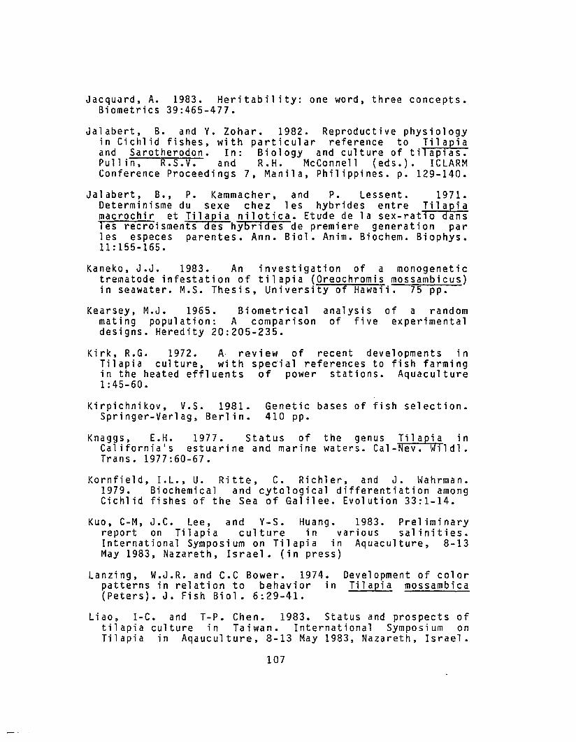
Jacquard, A. 1983. Heritability: one word, three concepts.Biometrics 39:465-477.
Ja1abert, B. and V. Zohar. 1982. Reproductive physiologyin Cich1id fishes, with particular reference to Ti1apiaand Sarotherodon. In: Biology and culture of tilapias.Pullin, R.S.V. and R.H. McConnell (eds.). ICLARMConference Proceedings 7, Manila, Philippines. p. 129-140.
Jalabert, B., P. Kammacher, and P. Lessent. 1971.Determinisme du sexe chez 1es hybrides entre Tilapiamacrochir et Ti1apia nilotica. Etude de 1a sex-ratio dansles recroisments des hy6rides de premiere generation parles especes parentes. Ann. Biol. Anim. Biochem. Biophys.11:155-165.
Kaneko, J.J. 1983. An investigation of a monogenetictrematode infestation of til apia (Oreochromis mossambicus)in seawater. M.S. Thesis, University of Hawaii. 75 pp.
Kearsey, M.J. 1965. Biometrica1mating population: A comparisondesigns. Heredity 20:205-235.
analysis of a randomof five experimental
Kirk, R.G. 1972. A· review of recent developments inTilapia culture, with special references to fish farmingin the heated effluents of power stations. Aquaculture1:45-60.
Kirpichnikov, V.S. 1981.Spri nger-Ver1 ag, Ber1 in.
Genetic bases of fish selection.410 pp.
Knaggs, E.H. 1977. Status of the genus Ti1apia inCa1ifornia 1s estuarine and marine waters. Cal-Nev. Wi1d1.Trans. 1977:60-67.
Kornfie1d, I.L., U. Ritte, C. Richler, and J. Wahrman.1979. Biochemical and cytological differentiation amongCich1id fishes of the Sea of Galilee. Evolution 33:1-14.
Kuo, C-M, J.C. Lee, and V-So Huang. 1983. Preliminaryreport on Ti1apia culture in various salinities.International Symposium on Ti1apia in Aquaculture, 8-13May 1983, Nazareth, Israel. (in press)
Lanzing, W.J.R. and C.C Bower. 1974.patterns in relation to behavior in(Peters). J. Fish Bio1. 6:29-41.
Development of colorTi1apia mossambica
Liao, I-C. and T-P. Chen. 1983. Status and prospects oftilapia culture in Taiwan. International Symposium onTilapia in Aqauculture, 8-13 May 1983, Nazareth, Israel.
107

(in press)
Liao, I-C. and S-L. Chang. 1983.feasibility of red tilapia cultureInternational Symposium on Tilapia inMay 1983, Nazareth, Israel. (in press)
Studies on thein saline water.Aquac ult ur e , 8-13
Ling, S-W. 1977. Aquaculture in Southeast Asia: Ahistorical overview. Washington Sea Grant Publication,contribution - College of Fisheries, Univ. of Washington:no. 465. 108 pp .
Lobel, P.S. 1980. Invasion by the Mozambique tilapia(Sarotherodon mossambicus; Pisces; Cichlidae) of a Pacificatoll marine ecosystem. Micronesica 16(2}:349-355.
Lowe-McConnell, R.H. 1982. Tilapias in fish communities.In: Biology and culture of tilapias. Pullin, R.S.V. andR.H. McConnell (eds.). ICLARM Conference Proceedings 7,Manila, Philippines. p, 83-113.
Maciolek, J.A. 1983. Exotic fishes in Hawaii and otherislands of Oceania. In: Distribution, biology, andmanagement of exotic fishes. Courtenay, W.R. Jr. and J.R.Stauffer (eds.). John Hopkins University Press. (in press)
Malecha, S. 1968. Studies on the serum proteinpolymorphisms in populations of introduced fresh waterfishes. M.S. Thesis, University of Hawaii. 122 pp.
Martin, J.W. 1967. Ajuvenile salmon from29:238-240.
method of measuringphotographs. Progr.
lengths ofFish-Cult.
Mi, M.P., S.M. Onizuka, and J.C. Wong. 1977. Computerprograms for statistical analysis of biomedical data.Cancer Center of Hawaii, Technical Report no. 5. 75 pp ,
Moav, R., T. Brody, G. Wohlfarth,Applications of electrophoreticbreeding. I. Advantages and9:217-228.
and G. Hulata. 1976.genetic markers to fishmethods. Aquaculture
Nei, M., T. Maruyama, and R. Chakraborty.bottleneck effect and genetic variability inEvolution 29:1-10.
1975. Thepopulations.
Pacific Islands Conference Standing Committee. 1981.Minutes of the Pacific Islands Conference StandingCommittee Meeting, Pago Pago, American Samoa, March 1981.
Pederson, D.G. 1972. A comparison of four experimental
108

designs for the estimation of heritability. Theor. Appl.Genet. 42:371-377.
Philippart, J-Cl. and J-Cl. Ruwet. 1982. Ecology anddistribution of tilapias. In: The biology and culture oftilapias. Pullin, R.S.V. and R.H. lowe-McConnell (eds.).IClARM Conference Proceedings 7, Manila, Philippines. p.15-59.
Pindyck, R.S. and D.L. Rubinfeld. 1981. Econometric modelsand economic forecasts. McGraw-Hill Book Co., New York.630 pp.
Pirsch, S. 1982. Buying fresh fish that is really fresh.Makai (UH Sea Grant Program) 4(9):3,5.
Pullin, R.S.V. 1982. General discussion on the biology andculture of tilapias. In: Biology and culture of tilapias.Pullin, R.S.V. and R.H. McConnell (eds.). ICLARMConference Proceedings 7, Manila, Philippines. p. 331-351.
Reagan, R.E., G.B. Pardue, and E.J. Eisen. 1976. Predictingselection response for growth of channel catfish. J. ofHeredity 67:49-53.
Refstie, T. and T.A. Steine. 1978. Selection experimentswith salmon. III. Genetic and environmental sources ofvariation in length and weight of Atlantic salmon in thefreshwater phase. Aquaculture 14:221-234.
Rothbard, S. and Y. Prugenin. 1975. Induced spawning andartificial incubation of Tilapia. Aquaculture 5:315-321.
Rothbard, S. and G. Hulata. 1980. Closed-system incubationfor Cichlid eggs. Progr. Fish-Cult. 42(4):203-204.
Schwartz, F.J. 1983. "Tilapia" hybrids: problems, values,use and world literature. International Symposium onTilapia in Aquaculture, 8-13 May 1983, Nazareth, Israel.(in press)
Shang, Y.C. and P. Macauley. 1981. Tilapia and Chinesecarp production and marketing in Hawaii: status andeconomic observations. Dept. of Planning and EconomicDevelopment, State of Hawaii. Mimeograph. 40 pp.
Silliman, R.P. 1975. Selective andexploitation of experimental populationsmossambica. Fish. Bull. 73(3):495-507.
unselectiveof Tilapia
Smith, L.S. 1982. Introduction to fish physiology. T.F.H.Publications, Inc., New Jersey. 352 pp.
109

Snedecor, G.W. and W.G. Cochran. 1967. Statisticalmethods. Iowa State Univ. Press, Ames, Iowa. 593 pp.
Tave, D. and R.O. Smitherman. 1980. Predicted response toselection for early growth in Tilapia nilotica. Trans. Am.Fish. Soc. 109:439-445.
Templeton, A.R. 1980. The theory of speciation via thefounder principle. Genetics 94:1011-1038.
Tietjen, G.l. and R.H. Moore. 1968. On testingsignificance of components of variance in the unbalancednested analysis of variance. Biometrics 24:423-429.
Trewavas, E. 1982a. Generic groupings of Tilapiini used inaquaculture. Aquaculture 27:79-81.
Trewavas, E. 1982b. Tilapias: Taxonomy and speciation. In:The biology and culture of tilapias. Pullin, R.S.V. andR.H. lowe-McConnell (eds.). IClARM Conference Proceedings7, Ma nil a, Phi 1 i ppin e s . p . 3- 13 •
Van Pel, H. 1955. Pond culture of tilapia. South PacificCommission Quarterly Bulletin 5(3): 30-31.
Von limbach, B. 1970. Fish genetics laboratory. Progressin sport fishery research. U.S. Fish Wildl. Servo ResourcePubl. 106:153-160.
Whitfield, A.K. and S.J.M. Blaber. 1979. The distributionof the freshwater cichlid Sarotherodon mossambicus inestuarine systems. Environ. Bio1. Fishes 4(1):77-81.
Wohlfarth, G.W. and G.L Hulata. 1981. Applied genetics oftilapias. ICLARM Studies and Reviews 6, Manila,Phil ippines. 26 pp ,
110