INFORMATION THEORY

CIS 400/628 — Spring 2005

Introduction to Cryptography

This is based on Chapter 15 of Trappe and Washington

SHANNON’S INFORMATION THEORY

I Late 1940s.

I Concerned with the amount of information, not whether it

is informative.

I Typical Problem: How much can we compress a message

and be able to reconstruct from the compressed version?

I Focus is on collections of messages and probabilities on them.

So common messages get short encodings and

uncommon ones get longer encodings.

— 1 —

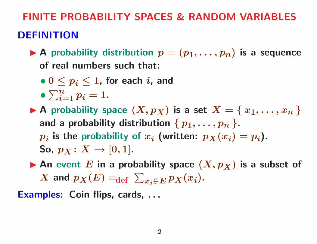
FINITE PROBABILITY SPACES & RANDOM VARIABLES

DEFINITION

I A probability distribution p = (p1, . . . , pn) is a sequence

of real numbers such that:

• 0 ≤ pi ≤ 1, for each i, and

•∑n

i=1 pi = 1.

I A probability space (X, pX) is a set X = { x1, . . . , xn }and a probability distribution { p1, . . . , pn }.

pi is the probability of xi (written: pX(xi) = pi).

So, pX : X → [0, 1].

I An event E in a probability space (X, pX) is a subset of

X and pX(E) =def∑

xi∈E pX(xi).

Examples: Coin flips, cards, . . .

— 2 —

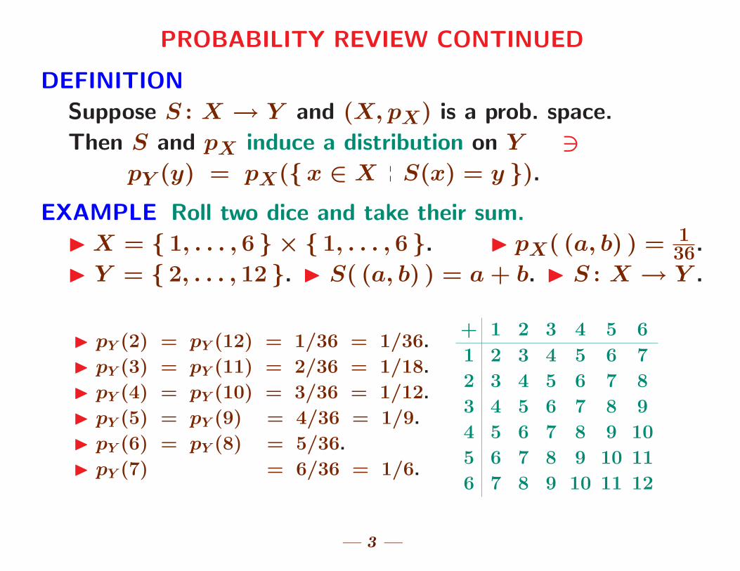
PROBABILITY REVIEW CONTINUED

DEFINITION

Suppose S : X → Y and (X, pX) is a prob. space.

Then S and pX induce a distribution on Y 3pY (y) = pX({ x ∈ X S(x) = y }).

EXAMPLE Roll two dice and take their sum.

I X = { 1, . . . , 6 } × { 1, . . . , 6 }. I pX( (a, b) ) = 136.

I Y = { 2, . . . , 12 }. I S( (a, b) ) = a + b. I S : X → Y .

I pY (2) = pY (12) = 1/36 = 1/36.

I pY (3) = pY (11) = 2/36 = 1/18.

I pY (4) = pY (10) = 3/36 = 1/12.

I pY (5) = pY (9) = 4/36 = 1/9.

I pY (6) = pY (8) = 5/36.

I pY (7) = 6/36 = 1/6.

+ 1 2 3 4 5 6

1 2 3 4 5 6 7

2 3 4 5 6 7 8

3 4 5 6 7 8 9

4 5 6 7 8 9 10

5 6 7 8 9 10 11

6 7 8 9 10 11 12

— 3 —

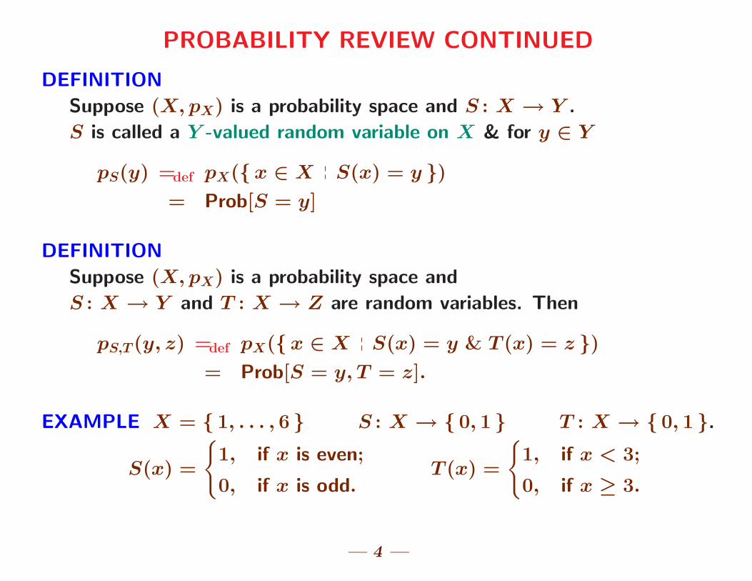
PROBABILITY REVIEW CONTINUED

DEFINITION

Suppose (X, pX) is a probability space and S : X → Y .

S is called a Y -valued random variable on X & for y ∈ Y

pS(y) =def pX({ x ∈ X S(x) = y })

= Prob[S = y]

DEFINITION

Suppose (X, pX) is a probability space and

S : X → Y and T : X → Z are random variables. Then

pS,T (y, z) =def pX({ x ∈ X S(x) = y & T (x) = z })

= Prob[S = y, T = z].

EXAMPLE X = { 1, . . . , 6 } S : X → { 0, 1 } T : X → { 0, 1 }.

S(x) =

{1, if x is even;

0, if x is odd.T (x) =

{1, if x < 3;

0, if x ≥ 3.

— 4 —

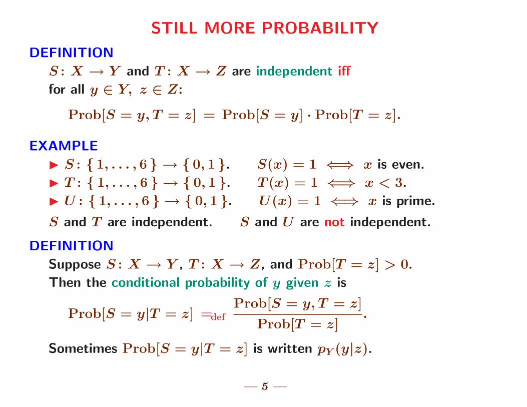
STILL MORE PROBABILITY

DEFINITION

S : X → Y and T : X → Z are independent iff

for all y ∈ Y, z ∈ Z:

Prob[S = y, T = z] = Prob[S = y] · Prob[T = z].

EXAMPLE

I S : { 1, . . . , 6 } → { 0, 1 }. S(x) = 1 ⇐⇒ x is even.

I T : { 1, . . . , 6 } → { 0, 1 }. T (x) = 1 ⇐⇒ x < 3.

I U : { 1, . . . , 6 } → { 0, 1 }. U(x) = 1 ⇐⇒ x is prime.

S and T are independent. S and U are not independent.

DEFINITION

Suppose S : X → Y , T : X → Z, and Prob[T = z] > 0.

Then the conditional probability of y given z is

Prob[S = y|T = z] =def

Prob[S = y, T = z]

Prob[T = z].

Sometimes Prob[S = y|T = z] is written pY (y|z).

— 5 —

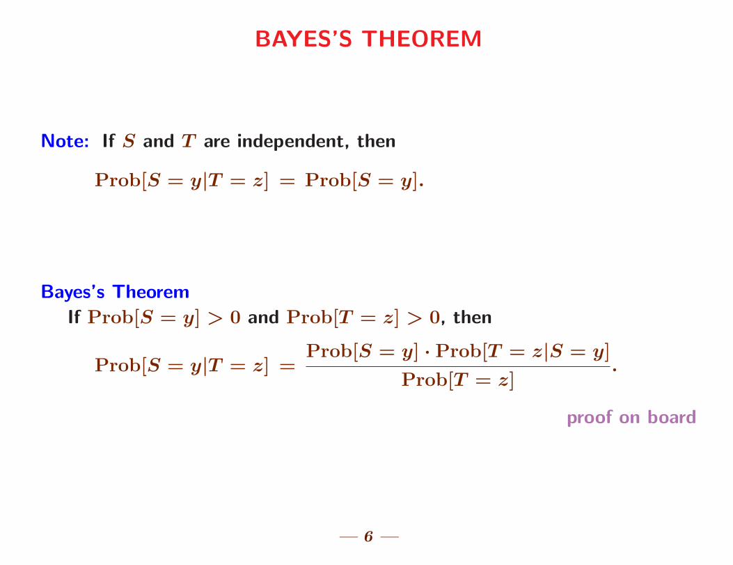
BAYES’S THEOREM

Note: If S and T are independent, then

Prob[S = y|T = z] = Prob[S = y].

Bayes’s Theorem

If Prob[S = y] > 0 and Prob[T = z] > 0, then

Prob[S = y|T = z] =Prob[S = y] · Prob[T = z|S = y]

Prob[T = z].

proof on board

— 6 —

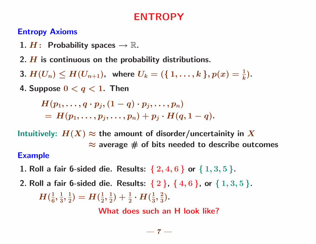
ENTROPY

Entropy Axioms

1. H : Probability spaces → R.

2. H is continuous on the probability distributions.

3. H(Un) ≤ H(Un+1), where Uk = ({ 1, . . . , k }, p(x) = 1k).

4. Suppose 0 < q < 1. Then

H(p1, . . . , q · pj, (1 − q) · pj, . . . , pn)

= H(p1, . . . , pj, . . . , pn) + pj · H(q, 1 − q).

Intuitively: H(X) ≈ the amount of disorder/uncertainity in X

≈ average # of bits needed to describe outcomes

Example

1. Roll a fair 6-sided die. Results: { 2, 4, 6 } or { 1, 3, 5 }.

2. Roll a fair 6-sided die. Results: { 2 }, { 4, 6 }, or { 1, 3, 5 }.

H(16, 1

3, 1

2) = H(1

2, 1

2) + 1

2· H(1

3, 2

3).

What does such an H look like?

— 7 —

MORE ON ENTROPY

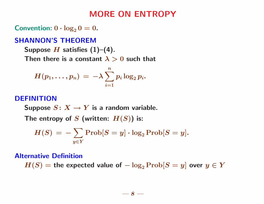
Convention: 0 · log2 0 = 0.

SHANNON’S THEOREM

Suppose H satisfies (1)–(4).

Then there is a constant λ > 0 such that

H(p1, . . . , pn) = −λ

n∑i=1

pi log2 pi.

DEFINITION

Suppose S : X → Y is a random variable.

The entropy of S (written: H(S)) is:

H(S) = −∑y∈Y

Prob[S = y] · log2 Prob[S = y].

Alternative Definition

H(S) = the expected value of − log2 Prob[S = y] over y ∈ Y

— 8 —

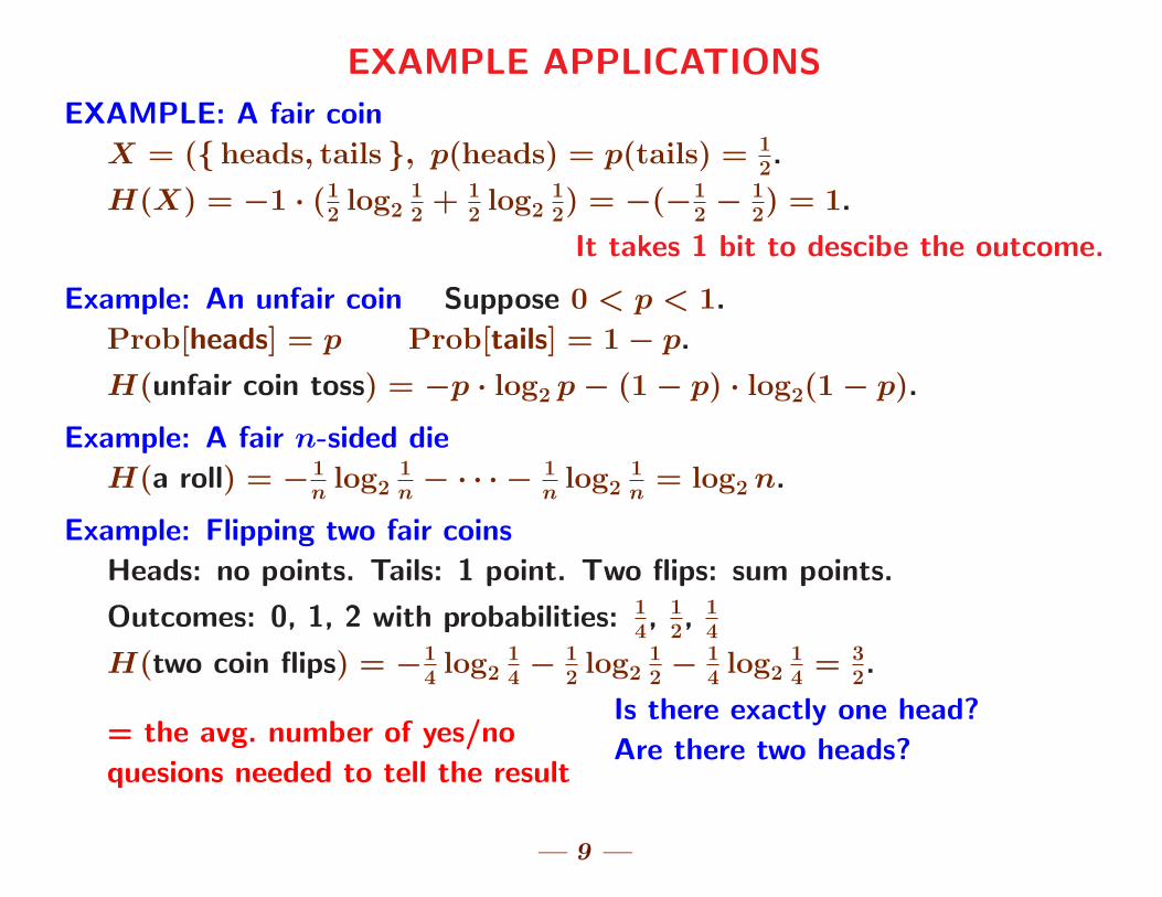
EXAMPLE APPLICATIONS

EXAMPLE: A fair coin

X = ({ heads, tails }, p(heads) = p(tails) = 12.

H(X) = −1 · (12log2

12+ 1

2log2

12) = −(−1

2− 1

2) = 1.

It takes 1 bit to descibe the outcome.

Example: An unfair coin Suppose 0 < p < 1.

Prob[heads] = p Prob[tails] = 1 − p.

H(unfair coin toss) = −p · log2 p − (1 − p) · log2(1 − p).

Example: A fair n-sided die

H(a roll) = −1nlog2

1n

− · · · − 1nlog2

1n

= log2 n.

Example: Flipping two fair coins

Heads: no points. Tails: 1 point. Two flips: sum points.

Outcomes: 0, 1, 2 with probabilities: 14, 1

2, 1

4

H(two coin flips) = −14log2

14

− 12log2

12

− 14log2

14

= 32.

= the avg. number of yes/no

quesions needed to tell the result

Is there exactly one head?

Are there two heads?

— 9 —

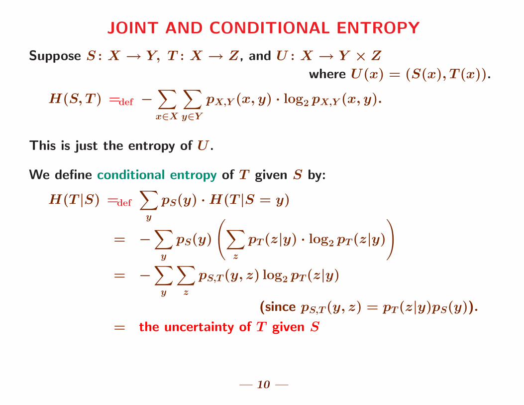
JOINT AND CONDITIONAL ENTROPY

Suppose S : X → Y, T : X → Z, and U : X → Y × Z

where U(x) = (S(x), T (x)).

H(S, T ) =def −∑x∈X

∑y∈Y

pX,Y (x, y) · log2 pX,Y (x, y).

This is just the entropy of U .

We define conditional entropy of T given S by:

H(T |S) =def

∑y

pS(y) · H(T |S = y)

= −∑

y

pS(y)

(∑z

pT (z|y) · log2 pT (z|y)

)= −

∑y

∑z

pS,T (y, z) log2 pT (z|y)

(since pS,T (y, z) = pT (z|y)pS(y)).

= the uncertainty of T given S

— 10 —

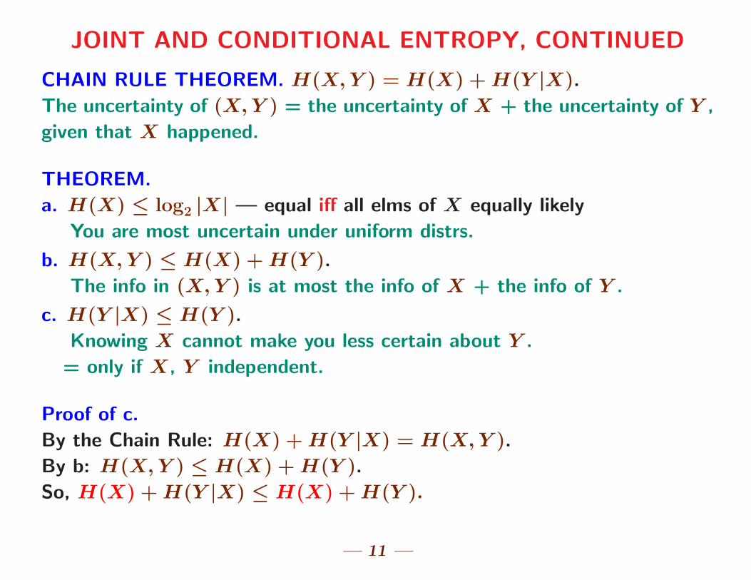
JOINT AND CONDITIONAL ENTROPY, CONTINUED

CHAIN RULE THEOREM. H(X, Y ) = H(X) + H(Y |X).

The uncertainty of (X, Y ) = the uncertainty of X + the uncertainty of Y ,

given that X happened.

THEOREM.

a. H(X) ≤ log2 |X| — equal iff all elms of X equally likely

You are most uncertain under uniform distrs.

b. H(X, Y ) ≤ H(X) + H(Y ).

The info in (X, Y ) is at most the info of X + the info of Y .

c. H(Y |X) ≤ H(Y ).

Knowing X cannot make you less certain about Y .

= only if X, Y independent.

Proof of c.

By the Chain Rule: H(X) + H(Y |X) = H(X, Y ).

By b: H(X, Y ) ≤ H(X) + H(Y ).

So, H(X) + H(Y |X) ≤ H(X) + H(Y ).

— 11 —

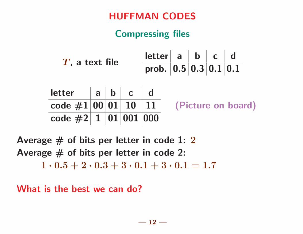
HUFFMAN CODES

Compressing files

T , a text fileletter a b c d

prob. 0.5 0.3 0.1 0.1

letter a b c d

code #1 00 01 10 11

code #2 1 01 001 000

(Picture on board)

Average # of bits per letter in code 1: 2

Average # of bits per letter in code 2:

1 · 0.5 + 2 · 0.3 + 3 · 0.1 + 3 · 0.1 = 1.7

What is the best we can do?

— 12 —

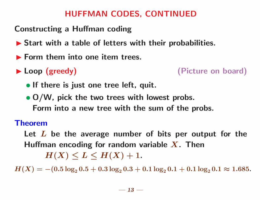
HUFFMAN CODES, CONTINUED

Constructing a Huffman coding

I Start with a table of letters with their probabilities.

I Form them into one item trees.

I Loop (greedy) (Picture on board)

• If there is just one tree left, quit.

• O/W, pick the two trees with lowest probs.

Form into a new tree with the sum of the probs.

Theorem

Let L be the average number of bits per output for the

Huffman encoding for random variable X. Then

H(X) ≤ L ≤ H(X) + 1.

H(X) = −(0.5 log2 0.5 + 0.3 log2 0.3 + 0.1 log2 0.1 + 0.1 log2 0.1 ≈ 1.685.

— 13 —

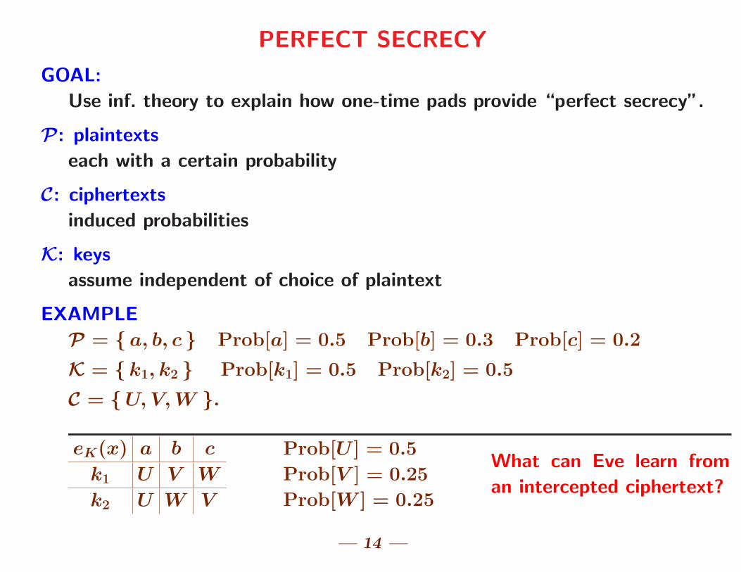
PERFECT SECRECY

GOAL:

Use inf. theory to explain how one-time pads provide “perfect secrecy”.

P: plaintexts

each with a certain probability

C: ciphertexts

induced probabilities

K: keys

assume independent of choice of plaintext

EXAMPLE

P = { a, b, c } Prob[a] = 0.5 Prob[b] = 0.3 Prob[c] = 0.2

K = { k1, k2 } Prob[k1] = 0.5 Prob[k2] = 0.5

C = { U, V, W }.

eK(x) a b c

k1 U V W

k2 U W V

Prob[U ] = 0.5

Prob[V ] = 0.25

Prob[W ] = 0.25

What can Eve learn from

an intercepted ciphertext?

— 14 —

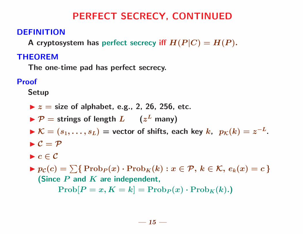
PERFECT SECRECY, CONTINUED

DEFINITION

A cryptosystem has perfect secrecy iff H(P |C) = H(P ).

THEOREM

The one-time pad has perfect secrecy.

Proof

Setup

I z = size of alphabet, e.g., 2, 26, 256, etc.

I P = strings of length L (zL many)

I K = (s1, . . . , sL) = vector of shifts, each key k, pK(k) = z−L.

I C = PI c ∈ CI pC(c) =

∑{ ProbP (x) · ProbK(k) : x ∈ P, k ∈ K, ek(x) = c }

(Since P and K are independent,

Prob[P = x, K = k] = ProbP (x) · ProbK(k).)

— 15 —

PROOF CONTINUED

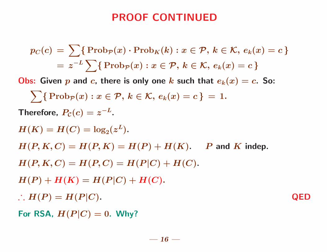
pC(c) =∑

{ ProbP(x) · ProbK(k) : x ∈ P, k ∈ K, ek(x) = c }

= z−L∑

{ ProbP(x) : x ∈ P, k ∈ K, ek(x) = c }

Obs: Given p and c, there is only one k such that ek(x) = c. So:∑{ ProbP(x) : x ∈ P, k ∈ K, ek(x) = c } = 1.

Therefore, PC(c) = z−L.

H(K) = H(C) = log2(zL).

H(P, K, C) = H(P, K) = H(P ) + H(K). P and K indep.

H(P, K, C) = H(P, C) = H(P |C) + H(C).

H(P ) + H(K) = H(P |C) + H(C).

∴ H(P ) = H(P |C). QED

For RSA, H(P |C) = 0. Why?

— 16 —

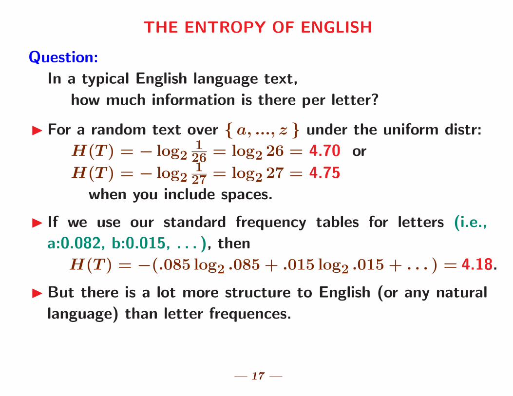
THE ENTROPY OF ENGLISH

Question:

In a typical English language text,

how much information is there per letter?

I For a random text over { a, ..., z } under the uniform distr:

H(T ) = − log2126 = log2 26 = 4.70 or

H(T ) = − log2127 = log2 27 = 4.75

when you include spaces.

I If we use our standard frequency tables for letters (i.e.,

a:0.082, b:0.015, . . . ), then

H(T ) = −(.085 log2 .085 + .015 log2 .015 + . . . ) = 4.18.

I But there is a lot more structure to English (or any natural

language) than letter frequences.

— 17 —

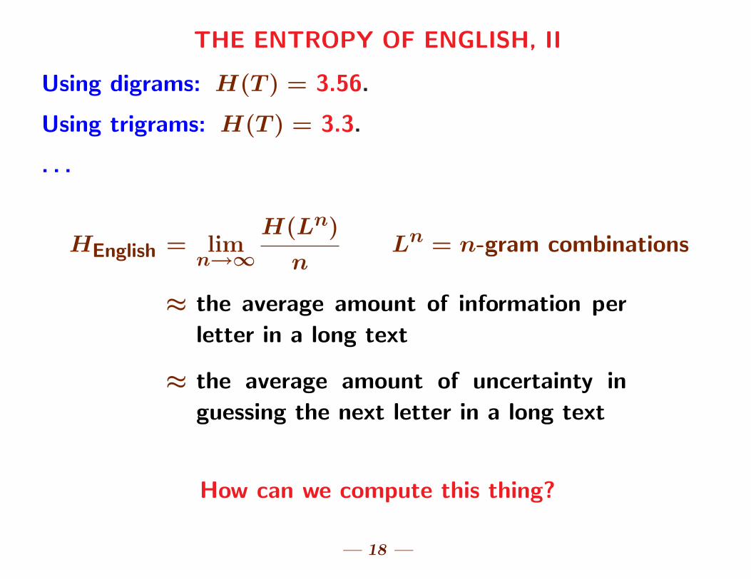
THE ENTROPY OF ENGLISH, II

Using digrams: H(T ) = 3.56.

Using trigrams: H(T ) = 3.3.

. . .

HEnglish = limn→∞

H(Ln)

nLn = n-gram combinations

≈ the average amount of information per

letter in a long text

≈ the average amount of uncertainty in

guessing the next letter in a long text

How can we compute this thing?

— 18 —

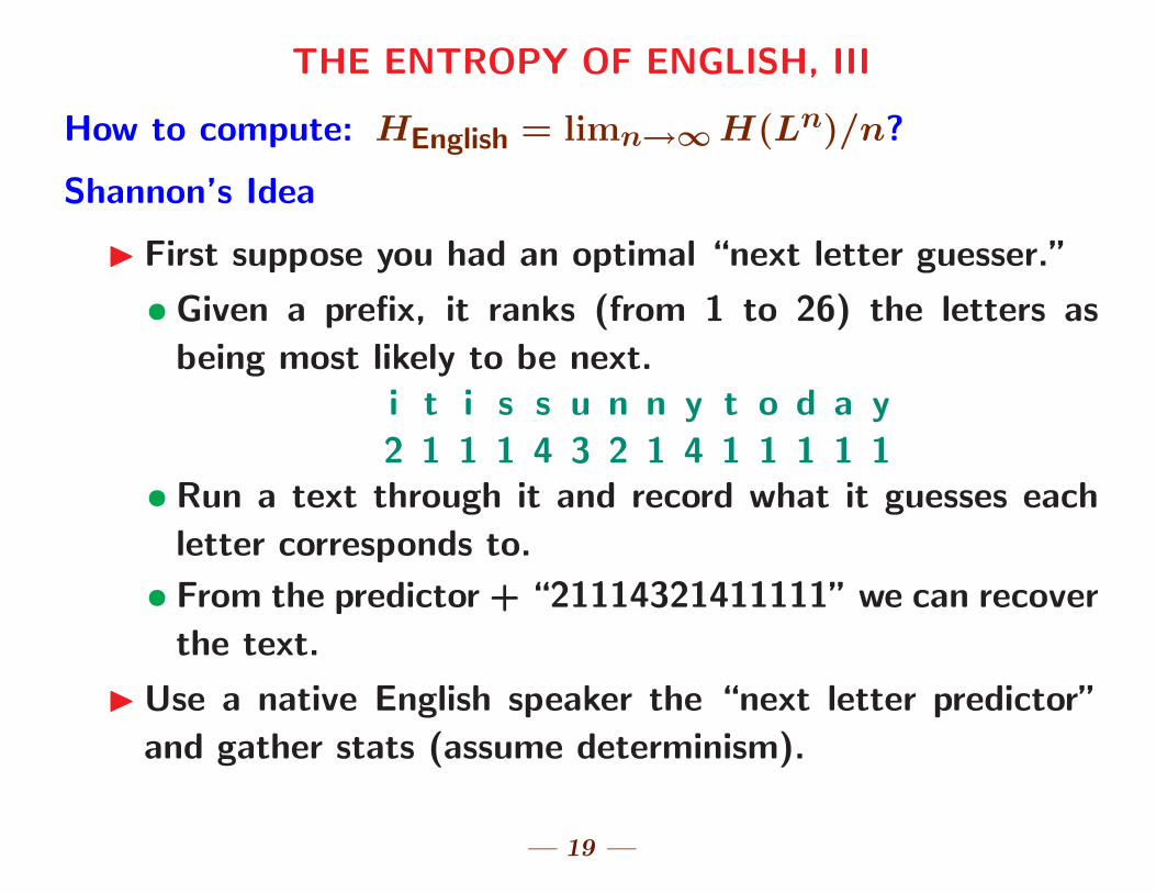
THE ENTROPY OF ENGLISH, III

How to compute: HEnglish = limn→∞ H(Ln)/n?

Shannon’s Idea

I First suppose you had an optimal “next letter guesser.”

• Given a prefix, it ranks (from 1 to 26) the letters as

being most likely to be next.i t i s s u n n y t o d a y

2 1 1 1 4 3 2 1 4 1 1 1 1 1• Run a text through it and record what it guesses each

letter corresponds to.

• From the predictor + “21114321411111” we can recover

the text.

I Use a native English speaker the “next letter predictor”

and gather stats (assume determinism).

— 19 —

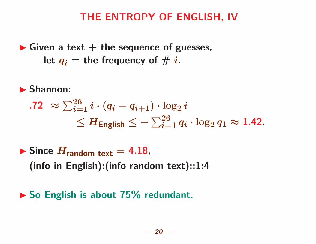
THE ENTROPY OF ENGLISH, IV

I Given a text + the sequence of guesses,

let qi = the frequency of # i.

I Shannon:

.72 ≈∑26

i=1 i · (qi − qi+1) · log2 i

≤ HEnglish ≤ −∑26

i=1 qi · log2 q1 ≈ 1.42.

I Since Hrandom text = 4.18,

(info in English):(info random text)::1:4

I So English is about 75% redundant.

— 20 —