1

Preprint version February 2001. This is the web version of this article, it is not completely identical tothe article published in Vision Research. Citation: Vision Res. 41:1851-1865 (2001)

Information theoretical evaluation of parametric models ofgain control in blowfly photoreceptor cells

J.H. van Hateren and H.P. Snippe

Department of Neurobiophysics, University of Groningen, Nijenborgh 4, NL-9747 AGGroningen, The Netherlands

Keywords: Light adaptation; Natural stimuli; Computational model

Summary

Models are developed and evaluated that are able to describe the response of blowflyphotoreceptor cells to natural time series of intensities. Evaluation of the models is performedusing an information theoretical technique that evaluates the performance of the models interms of a coherence function and a derived coherence rate (in bit/s). Performance is gaugedagainst a maximum expected coherence rate determined from the repeatability of the responseto the same stimulus. The best model performs close to this maximum performance, andconsists of a cascade of two divisive feedback loops followed by a static nonlinearity. Thefirst feedback loop is fast, effectively compressing fast and large transients in the stimulus.The second feedback loop also contains slow components, and is responsible for slowadaptation in the photoreceptor in response to large steps in intensity. Any remaining peaksthat would drive the photoreceptor out of its dynamic range are handled by the finalcompressive nonlinearity.

Introduction

Light intensities in the natural environment of an organism vary considerably. Not only long-term variations in light level are present, as those originating from the cycle of day and nightor from the change of seasons, but relatively large variations also occur on a much shortertime scale. This happens for example when moving through different sections of a landscape,such as going from open terrain into the shade of a group of trees. It also happens when theeye shifts its gaze from brightly lit parts of a scene to shaded areas. The photoreceptors of theeye therefore have to cope with variations in light level of at least 2-3 log units in relativelyshort stretches of time (van Hateren, 1997). This is more than the typical dynamic range ofneurons, with dynamic range defined here as the ratio of the maximum response and the noiselevel. To solve this problem, the photoreceptors of many, if not all, species can quickly adjusttheir gain to changing light levels. The purpose of the present article is to develop andevaluate models of this gain control in the photoreceptor cells of blowflies, and in particularmodels that are able to handle naturally occurring series of intensities.

There are at least three reasons why a model of photoreceptor gain control is useful: aphysiological, a practical, and a theoretical reason. The first, physiological, reason is thatmodelling can help to study the physiology of phototransduction and gain control, by pointingto key control loops and suggesting specific experiments. The second, practical, reason fordesiring a model of photoreceptor gain control is that it can serve as a preprocessing modulefor studying visual processing in higher parts of the visual system. More often than notsimple, linear processing is assumed for early visual processing. This induces the risk thateffects observed at a higher stage are interpreted as properties of that stage, whereas they mayin fact be the byproduct of nonlinearities in earlier stages. A full model of higher visualprocessing needs an adequate preprocessing model, including gain control at the earlieststages. The third, theoretical, reason for wanting a model of gain control is that this will be

2

necessary for understanding the relationship between the properties of natural stimuli andearly visual processing. In this approach, visual processing is considered to be optimallyadapted to the natural visual environment. Although much progress has been made in this areaby the application of information theory (Srinivasan, Laughlin & Dubs, 1982; Atick &Redlich, 1990; van Hateren, 1992), much of this assumes linear or quasi-linear systems, and agood nonlinear model will be instrumental to extend this approach to a more general range ofsystems.

At this point in time, there appears to be not yet sufficient information on blowflyphototransduction and light adaptation to produce a detailed physiological model that wouldwork adequately for the type of signals photoreceptors encounter in natural circumstances.Although such a model will ultimately become possible, it is likely to contain manyparameters given the complexity of the molecular machinery. For some purposes, a complexmodel is undesirable. Therefore, we will focus in this article on relatively simple models, withas few parameters as possible. These models will target in particular the second and thirdpurposes mentioned above: the final model will firstly serve as a preprocessing module usefulfor studies of higher stages of visual processing, and secondly it will help future studies ofunderstanding the information capacity of the early visual system.

For evaluating the various models we use a combination of several recently developedtechniques. As a stimulus, Natural Time Series of Intensities (called NTSIs below, vanHateren, 1997) are used, mimicking the statistics of the intensity as a function of time that isnormally encountered by individual photoreceptors. Responses from blowfly photoreceptorsto this stimulus were measured. From an inversion of the reconstruction method for obtaininginformation rates (Bialek, Rieke, de Ruyter van Steveninck & Warland, 1991; Theunissen,Roddey, Stufflebeam, Clague & Miller, 1996; Haag & Borst, 1997), combined with anonlinear model, a coherence function of stimulus and response is calculated. This cansubsequently be compared with an expected coherence function obtained by looking atresponse repeatability. As a result, the performance of the models can be evaluated as gaugedagainst the maximum performance that can be expected (Haag & Borst, 1997; Roddey, Girish& Miller, 2000). The best model we found, a cascade of two dynamic nonlinearities and astatic nonlinearity, is performing close to this maximum.

Methods

Stimuli and measurements

NTSIs were measured with a light detector worn on a headband by a person walking througha natural environment (van Hateren & van der Schaaf, 1996; van Hateren, 1997). The lightdetector had an acceptance angle of approximately 2 arcmin, and followed the pointingdirection of the face (see van Hateren, 1997, for further details). Obviously, the NTSIs thusmeasured are not identical to those that fly photoreceptor cells would normally encounter:many parameters, such as speed and behaviour of the organism, average distance to objects,and acceptance angle of the photoreceptors are quite different. It can be argued that several ofthese parameters cancel each other, and that scale-invariance of the environment will produceNTSIs for different organisms that are not as different as expected (van Hateren, 1997), butthis argument is not essential for the present study. Here it is only important that the stimulusis sufficiently complex, i.e., that it contains variations in intensity and contrast with the right(natural) mixture of predictability and unpredictability. These variations will then drive thephotoreceptor cells into regimes of gain control similar to those in which they function intruly natural circumstances. This makes the stimulus different from laboratory stimuli likesinusoids, flashes, and white noise, which are less complex (lower dimensional, in the sensethat they can be generated on the basis of only a few parameters). In van Hateren (1997) itwas shown that photoreceptors can handle the NTSIs quite well, and that stimulus andresponse are not linearly related.

The measured NTSIs were played back (at 1200 Hz) on a high-brightness LED, producinglight intensities comparable with daylight conditions (van Hateren, 1997). The LED produced

3

a wide-field stimulus of approximately 15 deg diameter; we found no change in responses forsmaller diameters as long as the stimulus covered the receptive field (approximately 2 deg indiameter) of the photoreceptor cell from which the membrane potential was measured. TheLED was driven by a D/A-convertor of a computer connected to a voltage-to-currentconvertor. The output of the LED was measured with a photodetector with a linear responsecharacteristic; this output was very similar to the original time series, showing only minornonlinearities in the LED and LED driver. For the analysis in this article, the measured LEDoutput was used as the NTSI, as this was the actual stimulus given to the photoreceptor. Themembrane potential of the photoreceptor cell was recorded by using an intracellularmicroelectrode, it was sampled at 1200 Hz, and stored for off-line analysis. The resultspresented here are based on 16 measurements in 7 photoreceptor cells of 4 blowflies(Calliphora vicina). For further details see van Hateren (1997).

Model evaluation

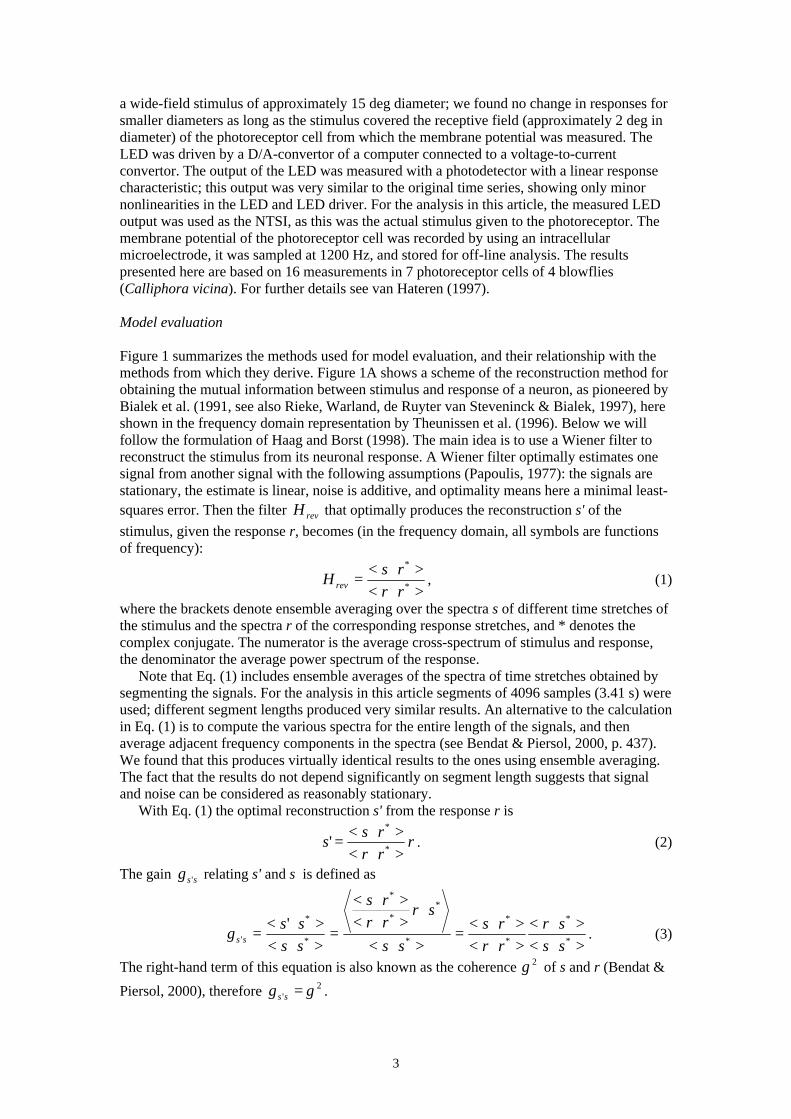
Figure 1 summarizes the methods used for model evaluation, and their relationship with themethods from which they derive. Figure 1A shows a scheme of the reconstruction method forobtaining the mutual information between stimulus and response of a neuron, as pioneered byBialek et al. (1991, see also Rieke, Warland, de Ruyter van Steveninck & Bialek, 1997), hereshown in the frequency domain representation by Theunissen et al. (1996). Below we willfollow the formulation of Haag and Borst (1998). The main idea is to use a Wiener filter toreconstruct the stimulus from its neuronal response. A Wiener filter optimally estimates onesignal from another signal with the following assumptions (Papoulis, 1977): the signals arestationary, the estimate is linear, noise is additive, and optimality means here a minimal least-squares error. Then the filter revH that optimally produces the reconstruction s' of the

stimulus, given the response r, becomes (in the frequency domain, all symbols are functionsof frequency):

>⋅<>⋅<

=*

*

rr

rsH rev , (1)

where the brackets denote ensemble averaging over the spectra s of different time stretches ofthe stimulus and the spectra r of the corresponding response stretches, and * denotes thecomplex conjugate. The numerator is the average cross-spectrum of stimulus and response,the denominator the average power spectrum of the response.

Note that Eq. (1) includes ensemble averages of the spectra of time stretches obtained bysegmenting the signals. For the analysis in this article segments of 4096 samples (3.41 s) wereused; different segment lengths produced very similar results. An alternative to the calculationin Eq. (1) is to compute the various spectra for the entire length of the signals, and thenaverage adjacent frequency components in the spectra (see Bendat & Piersol, 2000, p. 437).We found that this produces virtually identical results to the ones using ensemble averaging.The fact that the results do not depend significantly on segment length suggests that signaland noise can be considered as reasonably stationary.

With Eq. (1) the optimal reconstruction s' from the response r is

rrr

rss

>⋅<>⋅<

=*

*

' . (2)

The gain ssg ' relating s' and s is defined as

>⋅<>⋅<

>⋅<>⋅<

=>⋅<

⋅>⋅<>⋅<

=>⋅<>⋅<

=*

*

*

*

*

**

*

*

*

'

'

ss

sr

rr

rs

ss

srrr

rs

ss

ssg ss . (3)

The right-hand term of this equation is also known as the coherence 2γ of s and r (Bendat &

Piersol, 2000), therefore 2' γ=ssg .

4

From the symmetry of the equations, in particular Eq. (3), it is clear that a forwardformulation of the problem (Fig. 1B) leads to equivalent equations: the filter fwdH that

optimally produces a construction of the response r', given the stimulus s, is

>⋅<>⋅<

=*

*

ss

srH fwd , (4)

with

sss

srr

>⋅<>⋅<

=*

*

' (5)

and

2'*

*

*

*

*

*

'

'γ==

>⋅<>⋅<

>⋅<>⋅<

=>⋅<>⋅<

= ssrr grr

rs

ss

sr

rr

rrg . (6)

The simplest interpretation of 2γ is that it is the concatenation (in any order) of the forward

and reverse Wiener filters. If the system is linear and noise-free, 2γ would be 1 for allfrequencies (original signal perfectly recovered after subsequent forward and reverse Wiener

filtering). If 12 <γ then this is due either to noise or other unaccounted signal sources, or tononlinearities (Bendat & Piersol, 2000). Note that Eq. (6) shows that the coherence functionsthat follow from the methods of Figs. 1A and B are identical. For a thoughtful discussion ofthe relative merits of the forward and reverse techniques see Theunissen et al. (1996).

Figure 1C shows how we propose to extend the method of Fig. 1B to nonlinear systems.The assumption here is that the stimulus is transformed first by a nonlinear system (yieldingssys) or a nonlinear model (yielding smod). Both are assumed to be essentially noise-free, i.e., tohave an effective noise level small compared to the noise that is added in the final stepleading to the response r. This final step is assumed to be linear, and can thus be treated witha Wiener filter as above. The gain rrg ' is in this case the coherence between smod and r. Notethat the measured response, r, is the response to a single stimulus presentation, not an averageresponse (see General method).

The final method, shown in Fig. 1D, provides an independent way to obtain a coherencefunction, and is used in this article as a benchmark for evaluating the models used in themethod of Fig. 1C (see General method). Again all nonlinearities are assumed to be includedin the nonlinear system, and the final step is taken as linear with transfer function g andassumed additive noise, n, yielding

nsnsgr rsys +=+= . (7)

The coherence between ssys and r is then (again following Haag & Borst, 1998, we will call

this the expected coherence, 2expγ )

1

)(

)()(

)()(

**

*

***

***

****

****2

+=

>⋅<+>⋅<>⋅<

=

=>⋅<+>⋅<>⋅<

>⋅<>⋅<=

=>+⋅+<>⋅<

>⋅+<>+⋅<=

SNR

SNR

nnss

ss

nnssss

ssgssg

nsgnsgss

snsgnsgs

rr

rr

rrsyssys

syssyssyssys

syssyssyssys

syssyssyssysexpγ

(8)

assuming uncorrelated signal and noise, thus 0* >=⋅< nssys , and with the signal-to-noise

ratio, SNR, defined as the ratio of signal and noise power

>⋅<>⋅<

=*

*

nn

ssSNR rr . (9)

From Eq. (8) it follows that

5

2

2

1 exp

expSNRγ

γ−

= . (10)

The expected coherence function 2expγ is determined by the method of Fig. 1D, by first

estimating the SNR from a repetition of the stimulus and subsequently applying Eq. (8). TheSNR was estimated in the following way. Suppose that the stimulus is repeated m times,yielding photoreceptor responses )(tiρ (i=1..m); note that the response is given here as a

function of the time t. From these measured responses we obtain the average response

)(1

)(1

tm

tm

ii∑

=

= ρρ , (11)

and the deviations )(tiδ of the responses around the average

)()()( ttt ii ρρδ −= . (12)

Now we can compute )(ωr , the Fourier transform of )(tρ , and )(ωid , the Fourier

transform of )(tiδ ; r and id are functions of the frequencyω . From this the raw signal and

noise power spectra can be computed:*

raw rrS ⋅= (13)

∑=

⋅=m

iii dd

mN

1

*raw

1, (14)

where, as before, the brackets denote averages over time segments. Both rawS and rawN are

biased estimators, however. The quantity rawS is an overestimate of the power spectrum*rr ssS ⋅= of the actual signal rs , as used in Eq. (9). A simple example illustrating this

problem is when 0=S (i.e., when the photoreceptor output contains only noise), because forfinite m the individual responses (consisting only of noise here) are not likely to cancelexactly in the average. Hence 0raw >S , even if 0=S . Because part of the noise power is

thus mistaken for signal power, the estimated noise power rawN will be an underestimate of

the true noise power *nnN ⋅= as used in Eq. (9). Therefore, estimating the SNR as

rawraw / NS (as is often done) leads to an overestimate of the actual SNR. Here we correct for

this bias as follows. Analogous to Eq. (7), we write the observed responses as a sum)()()( ttt iri νσρ += (15)

of a noise-free signal rσ and a noise iν , assuming rσ and iν to be statistically independent.

Assuming also that the noises iν in the repetitions of the experiment are statistically

independent, the computed quantity rawS has a mathematical expectation

Nm

SS1ˆ

raw += . (16)

From Eqs. (11) and (15) we find

∑=

+=m

iir t

mtt

1

)(1

)()( νσρ , (17)

and consequently with Eqs. (12), (15) and (17)

∑∑≠==

−−=−=−+=m

ijj

ji

m

jjiiri mmm

t11

1)

11(

1)()( ννννρνσδ . (18)

6

Because )(ωid is the Fourier transform of )(tiδ , we find with Eq. (14) that the computed

quantity rawN has a mathematical expectation

Nm

mN

m

mN

mN

11)

11(ˆ

22

raw

−=

−+−= , (19)

again assuming that the noises iν are statistically independent. From Eqs. (16) and (19) it

follows that unbiased estimates N and S of N and S can be obtained as

raw1ˆ N

m

mN

−= (20)

rawrawraw 1

1ˆ1ˆ Nm

SNm

SS−

−=−= . (21)

Finally, from S and N an estimate of the SNR is obtained as

mN

S

m

m

N

SSNR

11ˆ

ˆ

raw

raw −−

== . (22)

For very large m, Eq. (22) reduces to the raw estimate rawraw / NS , but for small m it gives a

better estimate of the actual SNR.

The coherence rate

If signal and noise have Gaussian statistics, and are independent of each other, Shannon'sequation (Shannon, 1948) gives the information rate R in the channel as

dfSNRR )1(log0

2 += ∫∞

, (23)

with f the frequency. With Eq. (10) this gives an information rate

dfR exp )1(log 2

0

2 γ−−= ∫∞

. (24)

This quantifies, with a single number, how close the coherence function is to 1 over the entire

frequency range. The contribution of frequencies where 2expγ is close to 1 is very large, and it

is very small for frequencies where 2expγ is close to 0. It is a useful measure even when the

conditions for Shannon's equation (23) are not met. It then simply summarizes the coherencefunction in a way that is more meaningful than, for instance, the average of the coherencefunction over a particular frequency band. In the remainder of this article, this single numberwill be called the coherence rate cohR ; it is given in bit/s as it can be considered as an

approximation of the information rate. cohR is defined for any coherence 2γ as

dfRcoh )1(log 2

0

2 γ−−= ∫∞

. (25)

Using this definition and the term 'coherence rate' aims to avoid confusion with the trueinformation rate of the system.

The method of Fig. 1D yields the expected coherence 2expγ . Using this result for 2γ in Eq.

(25), we obtain the expected coherence rate, Rexp. It is in fact the expectation of the coherencebetween single responses ri and a noise-free system response ssys , where the latter isdetermined by averaging many responses. The result of this averaging can be considered asthe response that the best possible (non-linear) model should give. Any model that deviatesfrom this best possible one will show larger deviations from the measured responses, and thus

7

a coherence rate smaller than the coherence rate, Rexp, due to the method of Fig. 1D. Thisconclusion depends on whether the averaging is not biased by experimental artefacts such asdrift in the measurements during the course of the experiment. This appears not to be asignificant problem in the present experiments, as we found that the cross-correlation betweenstimulus and noise (as determined according to the method of Fig. 1D) is negligible. We alsodid not find a systematic change in noise level as a function of response level. Therefore, Rexp

can be considered as a target for the coherence rate, an upper bound against which coherencerates obtained through the method of Fig. 1C can be gauged. A variant of this method wasrecently used by Roddey et al. (2000) for investigating the performance of a linear model forreceptor cells in the cricket cercal system.

General method

The general method followed in this article is then as follows: for a given model, parameterswere fitted to maximize the coherence rate Rcoh for that model (Fig. 1C). This maximizationwas performed using a simplex algorithm (Press, Teukolsky, Vetterling & Flannery, 1992).Coherence rates were calculated with Eq. (25) by integrating up to 200 Hz; this frequencyrange includes virtually all signal power for blowfly photoreceptor cells. For the resultspresented below, the coherence functions and responses were calculated for the same fullstretch of 300 s data as was used for fitting the parameters of each model. To check againstoverfitting, we performed control computations where coherence rates were calculated for adifferent part of the time series than what was used for the fits, and found virtually identicalresults. Different models were investigated, each time maximizing Rcoh, in order to find amodel with Rcoh as close as possible to Rexp (Fig. 1D). The models presented below are in factthe most instructive or interesting results of this search through model space.

For evaluating the models of Fig. 1C we chose to use the response r to a single stimuluspresentation for calculating the coherence function with the model outcome. An alternativewould have been to use the average response to a large number of stimulus repeats. We didnot use this alternative because it would yield much higher coherence rates (because the noisewould be averaged out), which could not be compared with the results of the method of Fig.1D. Thus we would loose our benchmark. A potential advantage of using averages rather thatsingle responses is that it avoids that the models would try to fit the noise in the responses aswell as the signal. The control computations mentioned above already suggest that this effectdoes not occur here to any significant degree. It is also not to be expected because thestimulus is long (typically 300 s). Even if the model would manage to fit noise in oneparticular segment of the stimulus, this is likely to be punished by a decreased quality of fit inanother segment (where the stimulus and reponses might be roughly similar, but the noisewould most likely be different). In this respect a long stimulus is similarly effective inavoiding fitting noise as a much shorter stimulus repeated many times.

Results

Below we will first present results from models that contain no or only a static (memory-less)nonlinearity, subsequently from models with a dynamic nonlinearity, and finally fromcombinations of these. The longer-term behaviour is discussed next, and for the purpose ofsimulations a complete model, including a parametrization of the Wiener filter, is presented.

Models with a static nonlinearity

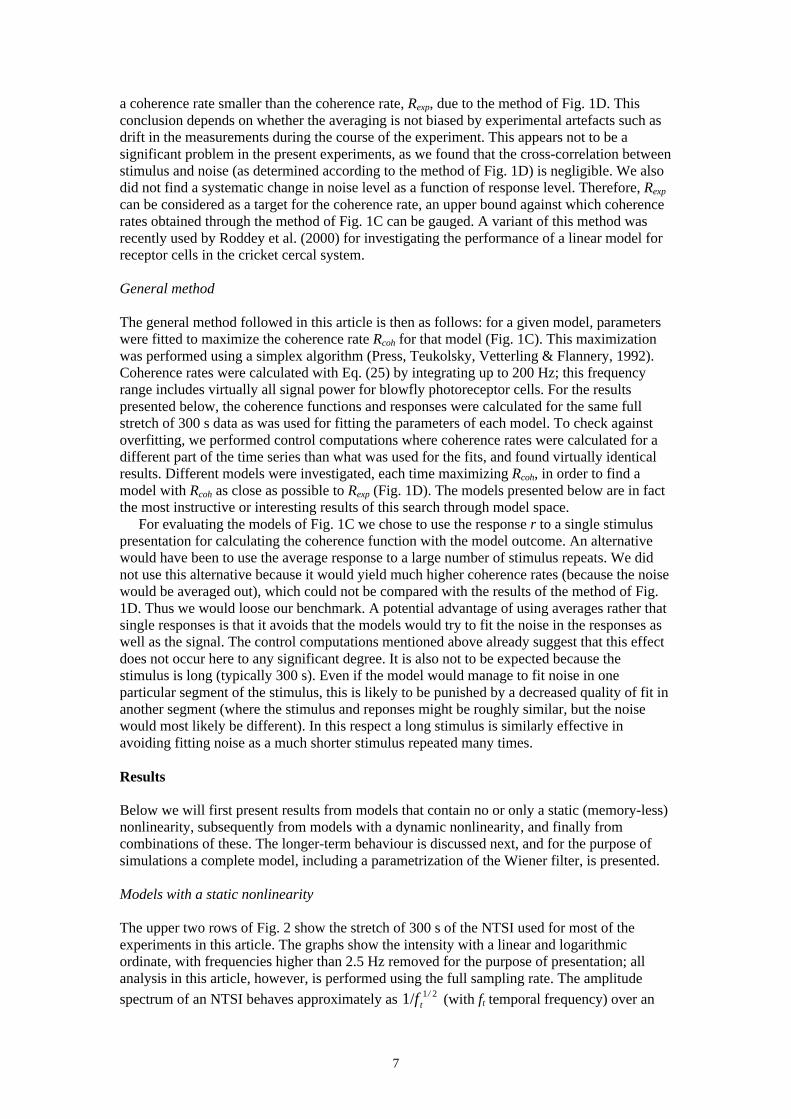
The upper two rows of Fig. 2 show the stretch of 300 s of the NTSI used for most of theexperiments in this article. The graphs show the intensity with a linear and logarithmicordinate, with frequencies higher than 2.5 Hz removed for the purpose of presentation; allanalysis in this article, however, is performed using the full sampling rate. The amplitude

spectrum of an NTSI behaves approximately as 211/ /tf (with ft temporal frequency) over an

8

appreciable frequency range (van Hateren, 1997). Thus low temporal frequencies dominatethe stimulus, although amplitudes at high frequencies are still appreciable because the fall-offwith frequency is relatively slow. The distribution of intensities is quite skew, with values athigh intensities sparser than at low intensities (Fig. 2, upper row); taking the logarithm of theintensity leads to a more symmetrical distribution (Fig. 2, second row). Further details on thestatistics can be found in van Hateren (1997).

The model results below are based on 16 measurements of the response of photoreceptorsto the NTSI shown in Fig. 2 (obtained from recordings of 7 photoreceptor cells in 4 flies). Theresponses shown in Figs. 2 and 4 are from a typical cell, which had a coherence rate andparameter values for model MDWN close to the average of the entire set of measurements.

The results of three simple models are shown in the third row and below of Fig. 2. Thefirst model, Mlin, contains no nonlinearities, so it just consists of the (linear) Wiener filter. Thethin line (red) shows the response of the photoreceptor cell, and the thick broken line (blue)the optimal Wiener prediction of the response. Both the total stretch of 300 s (limited to 2.5Hz) and three shorter sections of 500 ms (at full resolution) are shown. The shorter sectionsare taken from positions denoted by the vertical bars on the abscissa of the 300 s graph; thebar widths cover approximately the temporal extent of these sections. As is clear from thegraphs, the linear model is not performing very well: apart from large DC shifts, also theamplitude of fast modulations is not well predicted. This is also clear from the coherencefunction shown to the right (obtained through Eq. 6). A maximum coherence of 0.8 is in factnot particularly high: for a linear system it would correspond, via Eq. (10), to an SNR=4.

The second model shown in Fig. 2, Mlog, is doing much better. It consists of a staticnonlinearity, a logarithm, followed by a Wiener filter. The coherence function is nowapproximately 0.95 at low frequencies, corresponding to an SNR=19. A logarithm is a verysimple implementation of Weber's law: it gives equal responses to stimuli of equal contrast,i.e., stimuli which scale in proportion to the local (time-)average of the intensity. Thelogarithm is also closely related to the dynamic gain control module called 'Weber' below(MW).

The final model of Fig. 2, Msqrt, consists of a square-root nonlinearity followed by aWiener filter. Although it performs somewhat worse than Mlog, this is mainly due todiscrepancies at low frequencies (as can be seen in the 500 ms sections). The coherence athigher frequencies is similar to that of Mlog, which means that the coherence rate (Eq. 25) isnot much lower for Msqrt than for Mlog (see Performance of the models below). The square-root nonlinearity is closely related to the dynamic gain module called 'DeVries-Rose' below(MD).

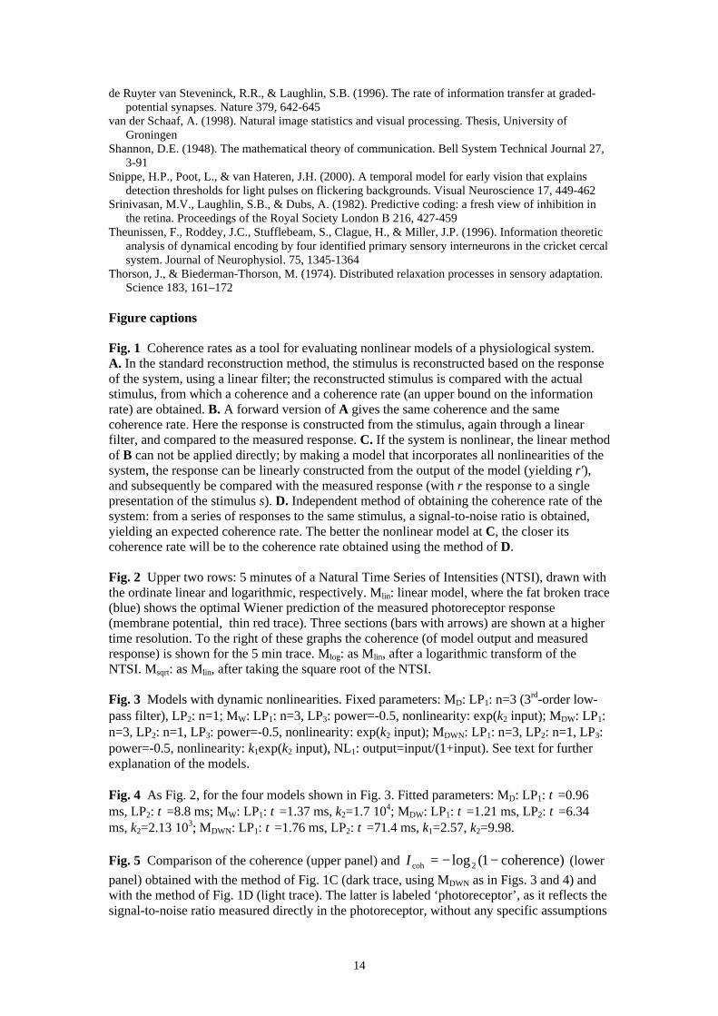
Models with a dynamic nonlinearity and cascaded models

Figure 3 shows schemes of several models that contain dynamic, rather than staticnonlinearities. These models are inspired by a recent model for light adaptation in the humanvisual system (Snippe, Poot & van Hateren, 2000). The upper two rows show models withonly a single control loop. The DeVries-Rose model, MD, contains a divisive feedback. Itssteady-state behaviour follows a square root, because for the steady state output=input/output,

thus output= input . A square-root scaling of sensitivity with luminance is commonly known

as the DeVries-Rose law, hence the model name. Note, however, that this behaviour of themodel is not caused by photon noise (a common cause of square-root behaviour), but is just aproperty of the feedback structure. Because of the low-pass filter LP2, the model producesovershoots at increment steps of the intensity, and undershoots at decrement steps. Figure 4,upper two rows, shows the performance of this model. Not surprisingly, it performs similarlyto Msqrt, although slightly better (see Performance of the models below).

The second model of Fig. 3 is the Weber model, MW, which contains an exponentialnonlinearity in the feedback loop. This is similar to Automatic Gain Control (AGC) systemsas used for regulating sound or video amplifiers (Ohlson, 1974). In the steady state it givesoutput=input/exp(output), which yields output ≈ log(input) if the scaling is chosen such that

9

log(output) << output. Therefore, an AGC loop has, like a pure logarithm, built-in Weberbehaviour. Although for AGC systems LP3 is usually taken as a first-order low-pass filter, itwas chosen here in a different way. When an intensity step is presented to a blowflyphotoreceptor, the response will, after an initial fast transient, continue to drop slowly forquite a long time (seconds to minutes). This long-term adaptation is in fact well matched tothe properties of NTSIs: these have power spectra that behave approximately as 1/ft (with ft

temporal frequency) over an appreciable range of frequencies (van Hateren, 1997; van derSchaaf, 1998). This means that NTSIs contain strong slow components, producing very longcorrelation times. If the underlying, 'local average' light intensity of such an NTSI would haveto be estimated, one possibility would be to weight the incoming intensities with a matched

filter (Papoulis, 1977), i.e., a filter with an amplitude characteristic ~ 211/ /tf . Although the

filter LP3 in Fig. 3 in fact operates on the model output rather than on the incomingintensities, this does not affect the basic idea since it is known (van Hateren, 1997) that, for

NTSIs, the actual photoreceptor output still behaves as approximately 211/ /tf . The filter LP3

in Fig. 3 is implemented as a superposition of first-order filters covering a range of timescales (Thorson & Biederman-Thorson, 1974). It is designated as 'power-law' because the

impulse response of a 211/ /tf -filter has a tail that declines as a power law of time (~ 211/ /t for a

minimum phase filter, see Kasdin, 1995). The filter is limited here to a total time span of 25 sto ensure it is integrable; changing this length by a factor of two had only small effects on theresults. Figure 4, second pair of rows, shows the performance of MW. It performs slightlyworse than MD.

The final two models schematized in Fig. 3 are cascades of two dynamic nonlinearitieswith (MDWN) and without (MDW) a final static nonlinearity. This static nonlinearity wasimplemented as a Naka-Rushton equation (output=input/(1+input)), but similar results wereobtained with an arctangent function as used before (Snippe et al., 2000). As Fig. 4 shows,both models perform quite well, better than any of the other models. The rms-deviationbetween model and measurement is slightly larger for the lowest response levels than forhigher ones: for MDWN the rms-deviation is 1.27 mV for responses <10 mV (4.5% of thedata), 0.92 mV for 10-15 mV (24%), 0.93 mV for 15-20 mV (28%), 0.87 mV for 20-25 mV(24%), 1.05 mV for 25-30 mV (17%), and 0.96 mV for responses >30mV (2.5%). A similartrend was found for the rms-deviation between model and measurement as a function ofstimulus intensity. In the next section we will investigate the relative overall performance ofthe models, and how well they compare to the maximum performance that can be expected.

Performance of the models

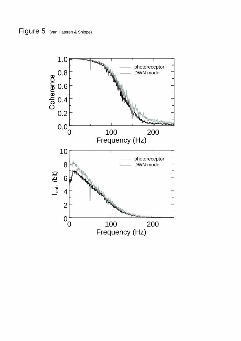
The coherence functions shown in Figs. 2 and 4 are those according to Eq. (6), following thescheme of Fig. 1C. They show the coherence between the measured response r and thenonlinear model prediction smod. An independent way to estimate a coherence function isthrough the scheme of Fig. 1D. The stimulus is here repeated many times, and only theresponses are subsequently studied. The signal power spectrum follows from the averageresponse, and the noise power spectrum from the average of the power spectra obtained fromthe difference between each individual response and the average response. From these spectrathe signal-to-noise ratio, SNR, can be obtained through Eq. (15). This subsequently yields,

through Eq. (8), an estimate of the expected coherence function, 2expγ . The expected

coherence function can be considered as an upper bound of the coherence function of thesystem (see Methods). As only the repeatability of the response is considered, there are noassumptions involved on a specific nonlinear model linking stimulus to response. Therefore,by comparing this with the coherence functions calculated for the models in Figs. 2 and 4, it ispossible to quantify how close the models are to the maximum coherence that can thus be

expected. Figure 5A shows an example of 2γ for MDWN (fat, blue line) and 2expγ (thin, red

line) determined for the same photoreceptor cell. As can be seen, they are quite close. An

10

alternative view of the performance is given by )1(log 22 γ−−=cohI , which is perhaps

more adequate because the coherence rate is the integral over cohI . From the resulting Fig. 5B

it is clear that the remaining discrepancies are mainly in the low-frequency part of cohI , but

that they are not very large.Although Fig. 5A shows that the coherence remains quite high up to frequencies as high as

70-80 Hz, this does not imply that this also holds for the SNR and cohI . The reason is that

coherences of similar magnitude, for example 0.99 and 0.95, can be associated with quitedifferent SNRs, in the example 99 and 19, respectively. As Fig. 5B shows, the performance ofthe photoreceptor to NTSIs already starts to decrease at frequencies of 20 Hz and up, at aboutthe same frequencies where the low-pass filtering of the photoreceptor starts to becomeapparent (van Hateren, 1997).

Integrating the curves in Fig. 5B over frequency gives two estimates of the coherence rate,

firstly the expected rate due to 2expγ , and secondly the coherence rate following from the 2γ

obtained from MDWN. These numbers were computed for all measurements and models, andthe results are shown in Fig. 6. The filled circles show the coherence rate obtained byaveraging the rates of the 16 measurements. Error bars show the s.e.m., with most of the barsfalling within the boundary of the circles. The coherence rate of the best model (MDWN) isonly slightly smaller than the expected coherence rate (open circle, average and s.e.m. of 8measurements with each typically 15 repeats; measurements were from 4 photoreceptors cellsof 3 blowflies).

Longer-term behaviour

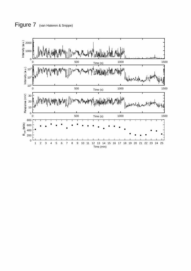
Most measurements were obtained with an NTSI of 5 min duration. A series of longerrecordings of 25 min were obtained as well (7 measurements from 6 cells in 3 flies), butintracellular recording time was not long enough to repeat this stimulus often enough to

obtain a reliable estimate of 2expγ . Nevertheless, using the model MDWN, it is possible to study

the coherence rate and how it varies over longer times. Figure 7 shows the 25 min stretch ofNTSI used (with the first 5 min identical to the NTSI of Fig. 2; graph limited to frequencieslower than 1 Hz). After about 1050 s the average intensity drops considerably, because forthis particular recording a wood was entered after walking through half-open countryside. Thethird row gives a typical photoreceptor response to this stimulus; this only gives a rough ideaof the response, however, because it had to be limited to frequencies lower than 1 Hz for thepurpose of presentation. Model MDWN was applied to each minute of this stimulus-responsepair, with different parameter settings fitted to each minute. From this the coherence rate ineach minute was calculated, which is shown in the lower graph (mean and s.e.m. of 7measurements). The coherence rate varies somewhat, but most when the average intensityvaries. The coherence rate averaged over the 25 minutes was 460 bit/s.

The performance of the various models when applied to the entire 25 min (thus now withparameters fixed for the entire period) is shown in Fig. 8. The model MDWN gives a coherencerate of 389±33 bit/s, appreciably smaller than the 460 bit/s found for separate minutes.Indeed, the parameters obtained from the fits to single minutes vary systematically, inparticular with the average light intensity of each minute. Figure 9 shows an attempt to takethis variation into account, by varying the time constant of the first filter, LP1, depending onthe output of filter LP3. The latter gives a rough, slowly varying estimate of the logarithm ofthe light intensity. Indeed, this model, Mτ, raises the coherence rate to 415±30 bit/s. Althoughthis may not seem significantly larger than the 389±33 bit/s of MDWN, this is masked by thevariation between cells: all 7 individual measurements gave an increased coherence rate, withan average increase of 7.4±2.3 %. Nevertheless, as this coherence rate still falls short of the460 bit/s average for single minutes, it is clear that model Mτ only captures part of the longer-term variations of photoreceptor cell functioning.

11

Models including a parametrization of the Wiener filter

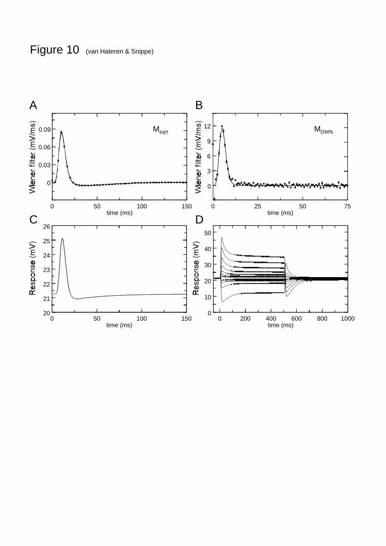
Although the models with static nonlinearities evaluated in Fig. 2 and the dynamic modelsshown in Fig. 3 take care of the nonlinearities in the system, they have to be followed by alinear filter (the Wiener filter) in order to completely specify the response of the system to aspecific stimulus. The Wiener filters that result from the analysis of the various models arefound in numerical form. For the purpose of evaluating the models or using them aspreprocessing modules in future studies of higher visual processing, it is more convenient tosummarize them with a simple function. We will do that here for two of the models, Msqrt andMDWN. The first is the simplest model that performs reasonably well for both the 5 and the 25minute NTSI (Figs. 6 and 8). Model MDWN is the overall top-performer. Figure 10A shows theWiener filter for Msqrt (dots) and its descriptive function (line). Figure 10B shows this forMDWN. Finally, Fig. 10C and D show the response of MDWN to several simple stimuli that haveoften been used for testing light-adapted photoreceptors: the responses to a very short pulseand to a series of 500 ms intensity steps of various magnitudes, both decrements andincrements. In the Discussion these model responses will be further assessed.

Discussion

In this article we used an information theoretical method to compare the performance of arange of models describing light adaptation and gain control in blowfly photoreceptor cells.The method makes it possible to gauge the performance of the models in terms of a coherencerate against an upper bound of a coherence rate that was estimated from the repeatability ofthe response to the same stimulus. The main conclusions are that nonlinearities are needed foran adequate model, and that dynamic nonlinearities perform better than static (memory-less)nonlinearities. Finally, for models describing longer-term behaviour additional control loops,adjusting for instance the time constants of the system, appear to be necessary.

The final model, MDWN, consists of a cascade of a fast feedback gain control loop, a slownonlinear feedback loop, and a static nonlinearity. The first feedback loop, behavingapproximately as a square-root device, will significantly reduce the considerable dynamicrange of the stimulus (short-term range 102-103) down to a size (10-30) that is manageable bythe physiology of the photoreceptor cell. Larger steps in stimulus intensity, occurringpredominantly on much slower time-scales, are handled by the second control loop,containing a power-law low-pass filter matching the time-scale invariance of NTSIs. Finally,any remaining peaks that would drive the photoreceptor cell out of its dynamic range, arehandled by the final static nonlinearity (van Hateren & Snippe, 2000). This combined systemkeeps the response well within the dynamic range of the photoreceptor cell, and produces acoherence rate close to the upper bound estimated from the repeatability of the response.

The number of fitted parameters is 4 for MDWN, with several more implicitly fixed by thechoice of filters and functional forms of nonlinearities. Clearly, the coherence rates followingfrom the progression of models in Figs. 2 and 4 increase with the number of parameters.Nevertheless, given the complexity and high dimensionality of the stimulus and response, thenumber of parameters is very modest in the nonlinear part of the models. Although the final(linear) Wiener filter does have many degrees of freedom, these do not contribute to thecoherence estimates. This can be readily shown from Eq. (6): multiplying s (or r) by anarbitrary linear filter F does not affect the coherence, because the effects of F in thenumerator and denominator of Eq. (6) cancel. The Wiener filter in the model only serves tominimize the root-mean-square deviations between the model outputs and the observedphotoreceptor response.

The MDWN model is similar to the first stage of the model by Snippe et al. (2000),developed for describing light adaptation and contrast gain control in the human visualsystem. The main difference is in the low-pass filter in the second control loop, which wastaken as a very slow first-order filter in Snippe et al. (in fact not dynamically active in theexperiments described there). Here it is modelled as a power-law low-pass filter, weighting

12

the incoming NTSI simultaneously over a range of time scales. The result is that adaptationworks over a range of time-scales, including quite slow ones. This is consistent with theobserved dynamics of fly photoreceptor adaptation.

Several of the components of the model have been used before by Lankheet, van Wezel,Prickaerts and van de Grind (1993) to describe gain control in horizontal cells in cat retina.They found that their results could be well described by a divisive feedback generating asquare-root behaviour, followed by a static nonlinearity. A difference with the MDWN modelevaluated here is that their model does not have the second, nonlinear feedback stage with apower-law low-pass filter. This module is used here to describe slow components in the gaincontrol.

French, Korenberg, Järvilehto, Kouvalainen, Juusola and Weckström (1993) developedmodels for predicting the response of blowfly photoreceptor cells to steps of intensity. Thesemodels consist of a cascade of static nonlinearities and a linear filter, thus somewhatresembling the models with static nonlinearities discussed in Fig. 2. Contrary to the presentstudy they subtract the DC-term from the membrane potential, and thus only study the rangeof temporal frequencies contained in intensity steps of 200 ms duration. It remains to bedetermined how well their class of models can perform with NTSIs, including variations inaverage light level on quite slow time-scales.

The responses predicted by the MDWN model to simple stimuli (Figs. 10C and D) arereasonably close to those measured before for light-adapted blowfly photoreceptors (French etal., 1993; Juusola, Kouvalainen, Järvilehto & Weckström, 1994). A discrepancy is that the V-logI curve of the model (DC membrane potential as a function of the logarithm of the lightintensity) is too shallow (Laughlin & Hardie, 1978). This is probably a major cause of thedependence of the rms-deviation on the response level (see Results). Nevertheless, theperformance of the model is quite good if one takes into account that it was in fact developedfor and tuned to an entire different class of stimuli (NTSIs). It is quite likely that carefuladjustment of the form of the various filters and nonlinearities in the model can significantlyimprove the reponse to stimuli as in Fig. 10, without deteriorating its performance withNTSIs.

Although the expected coherence rate found here (577±30 bit/s) should not be equatedwith the true information rate (see Methods), it is still interesting to compare these resultswith those obtained by de Ruyter van Steveninck and Laughlin (1996). They used white noisestimuli of much lower effective contrast, producing response amplitudes not exceeding a fewmillivolt. In that case the assumptions on linearity of the signal transfer and Gaussianproperties of the signals are better fullfilled than here, and the information rate they find forthis stimulus is roughly 400 bit/s (estimated from their Fig. 2). They subsequently extrapolatethis to higher contrasts, yielding 1000 bit/s. Given the assumptions involved in that procedure,and the non-Gaussian statistics of the stimuli used in the present study, it is clear that theirresults and those reported here are in essence consistent.

Coherence rates as a tool for model evaluation

The coherence and coherence rate were used here as a tool to evaluate the adequacy ofparticular models, as compared to an upper bound on the coherence rate obtained byanalyzing the repeatability of the response to the same stimulus. This method provides themodeller with a single number that summarizes how one model compares to another.Moreover, it also shows how far a model is from the final goal, a model equally adequate asthe system under consideration itself. Although this can also be accomplished by the moretraditional approach of calculating the root-mean-square difference between model predictionand measurement, we believe the present method has several advantages, in particular formodelling information processing systems. Deviations between model and measurement areweighted according to how much information the various frequency bands carry about thesignal. Furthermore, the resulting coherence rate has a simple interpretation in that it is anestimate of the information transferred by the system, be it that the estimate will be biased inthe case of non-Gaussian signals.

13

For the methods of Figs. 1C and D it was assumed that the nonlinear system could be splitin a deterministic part followed by an additive noise source. But we know that noise tends tobe generated at practically any stage of a real physiological system, thus it remains to be seenhow good this assumption is. For a system with distributed noise sources, it depends on thetype of nonlinearities how much of the resulting noise can in effect be considered as additive,rather than, for example, multiplicative.

Acknowledgements. We would like to thank Sietse van Netten en Doekele Stavenga foruseful comments. Portions of this work were presented at the annual meeting of theAssociation for Research in Vision and Ophthalmology (van Hateren & Snippe, 2000). Theresearch was supported by the Netherlands Organization for Scientific Research (NWO)through the Research Council for Earth and Lifesciences (ALW).

References

Atick, J.J., & Redlich, A.N. (1990). Towards a theory of early visual processing. Neural Computation2, 308-320

Bendat, J.S., & Piersol, A.G. (2000). Random data: analysis and measurement procedures. Thirdedition. Wiley-Interscience, New York

Bialek, W., Rieke, F., de Ruyter van Steveninck, R.R., & Warland, D. (1991). Reading a neural code.Science 252, 1854-1857

French, A.S., Korenberg, M.J., Järvilehto, M., Kouvalainen, E., Juusola, M., & Weckström, M. (1993).The dynamic nonlinear behavior of fly photoreceptors evoked by a wide rage of light intensities.Biophysical Journal 65, 832-839

Haag, J., & Borst, A. (1997) Encoding of visual motion information and reliability in spiking andgraded potential neurons. Journal of Neuroscience 17, 4809-4819

Haag, J., & Borst, A. (1998). Active membrane properties and signal encoding in graded potentialneurons. Journal of Neuroscience 18, 7972-7986

van Hateren, J.H. (1992). Theoretical predictions of spatiotemporal receptive fields of fly LMCs, andexperimental validation. Journal of Comparative Physiology A 171, 157-170

van Hateren, J.H., & van der Schaaf, A. (1996). Temporal properties of natural scenes. In: Proceedingsof the IS&T/SPIE Conference on Electronic Imaging: Science & Technology, Vol.2657 (pp.139-143). San Jose: SPIE

van Hateren, J.H. (1997). Processing of natural time series of intensities by the visual system of theblowfly. Vision Research 37, 3407-3416

van Hateren, J.H., & Snippe, H.P. (2000). A parametric model for the processing of natural time seriesof intensities by blowfly photoreceptor cells. Investigative Ophthalmology & Visual Science(Suppl.) 41, 492

Juusola, M., Kouvalainen, E., Järvilehto, M., & Weckström, M. (1994). Contrast gain, signal-to-noiseratio, and linearity in light-adapted blowfly photoreceptors. Journal of General Physiology 104,593-621

Kasdin, N.J. (1995). Discrete simulation of colored noise and stochastic processes and αf/1 power

law noise generation. Proceeding of the IEEE 83, 802-827Lankheet, M.J.M., van Wezel, R.J.A., Prickaerts, J.H.H.J., & van de Grind, W.A. (1993). The

dynamics of light adaptation in cat horizontal cell responses. Vision Research 33, 1153-1171Laughlin, S.B., & Hardie, R.C. (1978). Common strategies for light adaptation in the peripheral visual

systems of fly and dragonfly. Journal of Comparative Physiology 128, 319-340Ohlson, J.E. (1974). Exact dynamics of automatic gain control. IEEE Transactions on Communications

COM-22, 72-75Papoulis, A. (1977). Signal analysis. McGraw-Hill, New YorkPress, W.H., Teukolsky, S.A., Vetterling, W.T., & Flannery, B.P. (1992). Numerical recipes in Fortran.

Cambridge University Press, New YorkRieke, F., Warland, D., de Ruyter van Steveninck, R.R., & Bialek, W. (1997). Spikes: exploring the

neural code. MIT Press, CambridgeRoddey, J.C., Girish, B., & Miller, J.P. (2000) Assessing the performance of neural encoding models in

the presence of noise. Journal of Computational Neuroscience 8, 95-112

14

de Ruyter van Steveninck, R.R., & Laughlin, S.B. (1996). The rate of information transfer at graded-potential synapses. Nature 379, 642-645

van der Schaaf, A. (1998). Natural image statistics and visual processing. Thesis, University ofGroningen

Shannon, D.E. (1948). The mathematical theory of communication. Bell System Technical Journal 27,3-91

Snippe, H.P., Poot, L., & van Hateren, J.H. (2000). A temporal model for early vision that explainsdetection thresholds for light pulses on flickering backgrounds. Visual Neuroscience 17, 449-462

Srinivasan, M.V., Laughlin, S.B., & Dubs, A. (1982). Predictive coding: a fresh view of inhibition inthe retina. Proceedings of the Royal Society London B 216, 427-459

Theunissen, F., Roddey, J.C., Stufflebeam, S., Clague, H., & Miller, J.P. (1996). Information theoreticanalysis of dynamical encoding by four identified primary sensory interneurons in the cricket cercalsystem. Journal of Neurophysiol. 75, 1345-1364

Thorson, J., & Biederman-Thorson, M. (1974). Distributed relaxation processes in sensory adaptation.Science 183, 161–172

Figure captions

Fig. 1 Coherence rates as a tool for evaluating nonlinear models of a physiological system.A. In the standard reconstruction method, the stimulus is reconstructed based on the responseof the system, using a linear filter; the reconstructed stimulus is compared with the actualstimulus, from which a coherence and a coherence rate (an upper bound on the informationrate) are obtained. B. A forward version of A gives the same coherence and the samecoherence rate. Here the response is constructed from the stimulus, again through a linearfilter, and compared to the measured response. C. If the system is nonlinear, the linear methodof B can not be applied directly; by making a model that incorporates all nonlinearities of thesystem, the response can be linearly constructed from the output of the model (yielding r'),and subsequently be compared with the measured response (with r the response to a singlepresentation of the stimulus s). D. Independent method of obtaining the coherence rate of thesystem: from a series of responses to the same stimulus, a signal-to-noise ratio is obtained,yielding an expected coherence rate. The better the nonlinear model at C, the closer itscoherence rate will be to the coherence rate obtained using the method of D.

Fig. 2 Upper two rows: 5 minutes of a Natural Time Series of Intensities (NTSI), drawn withthe ordinate linear and logarithmic, respectively. Mlin: linear model, where the fat broken trace(blue) shows the optimal Wiener prediction of the measured photoreceptor response(membrane potential, thin red trace). Three sections (bars with arrows) are shown at a highertime resolution. To the right of these graphs the coherence (of model output and measuredresponse) is shown for the 5 min trace. Mlog: as Mlin, after a logarithmic transform of theNTSI. Msqrt: as Mlin, after taking the square root of the NTSI.

Fig. 3 Models with dynamic nonlinearities. Fixed parameters: MD: LP1: n=3 (3rd-order low-pass filter), LP2: n=1; MW: LP1: n=3, LP3: power=-0.5, nonlinearity: exp(k2⋅input); MDW: LP1:n=3, LP2: n=1, LP3: power=-0.5, nonlinearity: exp(k2⋅input); MDWN: LP1: n=3, LP2: n=1, LP3:power=-0.5, nonlinearity: k1exp(k2⋅input), NL1: output=input/(1+input). See text for furtherexplanation of the models.

Fig. 4 As Fig. 2, for the four models shown in Fig. 3. Fitted parameters: MD: LP1: τ =0.96ms, LP2: τ =8.8 ms; MW: LP1: τ =1.37 ms, k2=1.7⋅104; MDW: LP1: τ =1.21 ms, LP2: τ =6.34ms, k2=2.13⋅103; MDWN: LP1: τ =1.76 ms, LP2: τ =71.4 ms, k1=2.57, k2=9.98.

Fig. 5 Comparison of the coherence (upper panel) and )coherence1(log 2coh −−=I (lower

panel) obtained with the method of Fig. 1C (dark trace, using MDWN as in Figs. 3 and 4) andwith the method of Fig. 1D (light trace). The latter is labeled ‘photoreceptor’, as it reflects thesignal-to-noise ratio measured directly in the photoreceptor, without any specific assumptions

15

on a model. It gives an upper bound on the coherence that can only be reached by themodelling method of Fig. 1C if both the nonlinear model is adequate and the assumptionsunderlying the method are correct.

Fig. 6 The coherence rate for a 5 min NTSI of the models evaluated in Figs. 2 and 4,compared to the direct estimation of Fig. 1D (labeled ‘photoreceptor’). Average and s.e.m. of16 measurements (models) and 8 measurements (‘photoreceptor’). Several error bars are notvisible because they fall within the extent of the dots.

Fig. 7 An NTSI of 25 min (upper two panels), an example of the response of a photoreceptorto this stimulus (third panel, limited to 1 Hz for the purpose of presentation), and thecoherence rate of model MDWN evaluated for consecutive minutes (lower panel; average ands.e.m. of 7 measurements).

Fig. 8 The coherence rate for a 25 min NTSI of the models evaluated in Figs. 2 and 4,compared to the average rate obtained by fitting MDWN to each minute separately (data pointsof Fig. 7, lower panel).

Fig. 9 Mτ, a modification of MDWN with a variable time constant of the first low-pass filter.Fixed parameters: LP1: n=3, LP2: n=1, LP3: power=-0.5, nonlinearity: k1exp(k2⋅input), NL1:output=input/(1+input), NL2: τ1 =τ0/(input)w. Fitted parameters for the measurement of Fig. 7,third row: LP1: τ1 output of NL2, with τ0 =0.28 ms, LP2: τ =43.3 ms, k1=8.18, k2=7.18,w=1.52.

Fig. 10 A. Wiener filter and its parametric model fit for Msqrt. The dots and error bars showthe average Wiener filter and the s.e.m. of 16 measurements, the line shows a fit with the

function )/exp()/()/exp()/( 22211121 ττττ ttAttA nn −−− , with A1=1.85⋅10-7 mV/ms,

τ1=1.133 ms, n1=10, A2=2.30⋅10-4 mV/ms, τ2=8.50 ms, n2=5. For the sake of clarity only 1 in

4 dots is shown. B. As A, for model MDWN; the fit is given by )/exp()/( ττ ttA n − , with

A=2.46⋅10-6 mV/ms, τ=0.535 ms, n=11. C. Pulse response of MDWN (including the parametricWiener filter) based on the model fit to one of the measured photoreceptor cells. Parametersof the Wiener filter: A=3.13⋅10-6 mV/ms, τ=0.535 ms, n=11; further model parameters LP1: τ=1.69 ms, LP2: τ =71.8 ms, k1=0.689, k2=9.07. D. Responses of MDWN to 500 ms steps in lightintensity, parameters as in C. Contrast steps: -0.8, -0.4, -0.2, -0.1, 0.1, 0.2, 0.4, 0.8, 1.6, 3.2,6.4.

Reversestimulus s

response r Wienerfilter

reconstructedstimulus 's

Forward

Nonlinear

SNR ofresponse

stimulus s

response r

Wienerfilter

constructedresponse r'

stimulus s

response r

Wienerfilter

constructedresponse r'

nonlinearmodel

nonlinearsystem

.....

gain(s,s')=

coherence rate

gain(r,r')

coherence rate

SNR

vary nonlinearmodel untilR Rcoh exp≈

Figure 1 (van Hateren & Snippe)

transformedstimulus ssys

transformedstimulus smod

gain(r,r')

coherence rate Rcoh

stimulus s

nonlinearsystem

transformedstimulus ssys

A

B

C

Dstimulus s

nonlinearsystem

transformedstimulus ssys

coherence( )s,r

=coherence( )s,r

=coherence( )s ,rmod

coherence( )s ,rsys

expected

coherence rate Rexp

expected

0 100 200 300Time (s)0

25

50

750 100 200 300Time (s)

102

103

0 100 200 300Time (s)0

1000

2000

3000

0 100 200 300Time (s)

10

20

30

0 100 200 300Time (s)0

20

40

0 100 200 300 400 500Time (ms)

10

20

30

40

0 100 200 300 400 500Time (ms)

0

10

20

30

0 100 200 300 400 500Time (ms)

10

20

30

40

0 100 200 300 400 500Time (ms)

20

30

40

50

60

0 100 200 300 400 500Time (ms)

0

10

20

30

0 100 200 300 400 500Time (ms)

0

10

20

30

40

0 100 200 300 400 500Time (ms)

20

30

40

50

0 100 200 300 400 500Time (ms)

5

10

15

20

25

0 100 200 300 400 500Time (ms)

10

20

30

40

Ilin

Ilog

Mlin

Mlog

Msqrt

0 100 200Frequency (Hz)

0.0

0.2

0.4

0.6

0.8

1.0

0 100 200Frequency (Hz)

0.0

0.2

0.4

0.6

0.8

1.0

0 100 200Frequency (Hz)

0.0

0.2

0.4

0.6

0.8

1.0

photoreceptormodel

Figure 2 (van Hateren & Snippe)

LP2

I(t) P(t)LP1

M : De Vries-RoseD

LP3

I(t) P(t)LP1

M : WeberW

LP2 LP3

I(t) P(t)LP1

M : De Vries-Rose & WeberDW

LP2 LP3

NL1I(t) P(t)LP1

M : De Vries-Rose & Weber & NLDWN

Figure 3 (van Hateren & Snippe)

MDW

MDWN

MW

Time (s)MD

photoreceptormodel

0 100 200 3000

20

40

0 100 200 300Time (s)0

20

40

0 100 200 300Time (s)

10

20

30

40

0 100 200 300Time (s)

10

20

30

0 100 200 300 400 500Time (ms)

20

30

40

50

0 100 200 300 400 500Time (ms)

5

10

15

20

25

0 100 200 300 400 500Time (ms)

10

20

30

40

0 100 200Frequency (Hz)

0.0

0.2

0.4

0.6

0.8

1.0

0 100 200 300 400 500Time (ms)

20

30

40

50

0 100 200 300 400 500Time (ms)

5

10

15

20

25

0 100 200 300 400 500Time (ms)

10

20

30

40

0 100 200Frequency (Hz)

0.0

0.2

0.4

0.6

0.8

1.0

0 100 200 300 400 500Time (ms)

20

30

40

0 100 200 300 400 500Time (ms)

5

10

15

20

25

0 100 200 300 400 500Time (ms)

10

20

30

40

0 100 200Frequency (Hz)

0.0

0.2

0.4

0.6

0.8

1.0

0 100 200 300 400 500Time (ms)

20

25

30

35

0 100 200 300 400 500Time (ms)

5

10

15

20

25

0 100 200 300 400 500Time (ms)

10

20

30

40

0 100 200Frequency (Hz)

0.0

0.2

0.4

0.6

0.8

1.0

Figure 4 (van Hateren & Snippe)

0 100 200Frequency (Hz)

0.0

0.2

0.4

0.6

0.8

1.0

0 100 200Frequency (Hz)

0

2

4

6

8

10

photoreceptorDWN model

photoreceptorDWN model

Figure 5 (van Hateren & Snippe)

Model

0

200

400

600

lin DWNDWlogDsqrtW

models

photoreceptor

Figure 6 (van Hateren & Snippe)

Time (s)

Time (s)0 500 1000 15000

1000

2000

0 500 1000 1500101

102

103

Figure 7 (van Hateren & Snippe)

0 500 1000 15000

10

20

30

Time (s)

1 2 3 4 5 6 7 8 9 10 11 12 13 14 15 16 17 18 19 20 21 22 23 24 25Time (min)

0

200

400

600

800

Figure 8 (van Hateren & Snippe)

Model

0

200

400

600

lin DWNDWlogDsqrtW τ

models (25 min)

separate minutes

LP2 LP3

NL1I(t) P(t)LP1

NL2

Figure 9 (van Hateren & Snippe)

0 50 100 150time (ms)

0

0.03

0.06

0.09

0 25 50 75time (ms)

0

3

6

9

12

0 50 100 150time (ms)

20

21

22

23

24

25

26

0 200 400 600 800 1000time (ms)

0

10

20

30

40

50

Msqrt MDWN

A

C D

B

Figure 10 (van Hateren & Snippe)