Embed Size (px)
Citation preview
Information-Theoretic Co-clustering
Inderjit S. DhillonDept. of Computer SciencesUniversity of Texas, Austin
Subramanyam MallelaDept. of Computer SciencesUniversity of Texas, Austin
Dharmendra S. ModhaIBM Almaden Research Center
San Jose, CA
ABSTRACTTwo-dimensional contingency or co-occurrence tables arisefrequently in important applications such as text, web-logand market-basket data analysis. A basic problem in contin-gency table analysis is co-clustering: simultaneous clusteringof the rows and columns. A novel theoretical formulationviews the contingency table as an empirical joint probabil-ity distribution of two discrete random variables and posesthe co-clustering problem as an optimization problem in in-formation theory — the optimal co-clustering maximizes themutual information between the clustered random variablessubject to constraints on the number of row and columnclusters. We present an innovative co-clustering algorithmthat monotonically increases the preserved mutual informa-tion by intertwining both the row and column clusteringsat all stages. Using the practical example of simultaneousword-document clustering, we demonstrate that our algo-rithm works well in practice, especially in the presence ofsparsity and high-dimensionality.
Categories and Subject DescriptorsE.4 [Coding and Information Theory]: Data compactionand compression; G.3 [Probability and Statistics]: Con-tingency table analysis; H.3.3 [Information Search andRetrieval]: Clustering; I.5.3 [Pattern Recognition]: Clus-tering
KeywordsCo-clustering, information theory, mutual information
1. INTRODUCTIONClustering is a fundamental tool in unsupervised learningthat is used to group together similar objects [14], and haspractical importance in a wide variety of applications suchas text, web-log and market-basket data analysis. Typically,the data that arises in these applications is arranged as acontingency or co-occurrence table, such as, word-documentco-occurrence table or webpage-user browsing data. Mostclustering algorithms focus on one-way clustering, i.e., clus-ter one dimension of the table based on similarities along thesecond dimension. For example, documents may be clus-tered based upon their word distributions or words may beclustered based upon their distribution amongst documents.
Permission to make digital or hard copies of all or part of this work forpersonal or classroom use is granted without fee provided that copies arenot made or distributed for profit or commercial advantage and that copiesbear this notice and the full citation on the first page. To copy otherwise, orrepublish, to post on servers or to redistribute to lists, requires prior specificpermission and/or a fee. SIGKDD ’03, August 24-27, 2003, Washington,DC, USA. Copyright 2003 ACM 1-58113-737-0/03/0008...$5.00.
It is often desirable to co-cluster or simultaneously clusterboth dimensions of a contingency table [11] by exploiting theclear duality between rows and columns. For example, wemay be interested in finding similar documents and their in-terplay with word clusters. Quite surprisingly, even if we areinterested in clustering along one dimension of the contin-gency table, when dealing with sparse and high-dimensionaldata, it turns out to be beneficial to employ co-clustering.
To outline a principled approach to co-clustering, we treatthe (normalized) non-negative contingency table as a jointprobability distribution between two discrete random vari-ables that take values over the rows and columns. We defineco-clustering as a pair of maps from rows to row-clustersand from columns to column-clusters. Clearly, these mapsinduce clustered random variables. Information theory cannow be used to give a theoretical formulation to the prob-lem: the optimal co-clustering is one that leads to the largestmutual information between the clustered random variables.Equivalently, the optimal co-clustering is one that minimizesthe difference (“loss”) in mutual information between theoriginal random variables and the mutual information be-tween the clustered random variables. In this paper, wepresent a novel algorithm that directly optimizes the aboveloss function. The resulting algorithm is quite interesting:it intertwines both row and column clustering at all stages.Row clustering is done by assessing closeness of each rowdistribution, in relative entropy, to certain “row cluster pro-totypes”. Column clustering is done similarly, and this pro-cess is iterated till it converges to a local minimum. Co-clustering differs from ordinary one-sided clustering in thatat all stages the row cluster prototypes incorporate columnclustering information, and vice versa. We theoretically es-tablish that our algorithm never increases the loss, and so,gradually improves the quality of co-clustering.
We empirically demonstrate that our co-clustering algorithmalleviates the problems of sparsity and high dimensionalityby presenting results on joint word-document clustering. Aninteresting aspect of the results is that our co-clustering ap-proach yields superior document clusters as compared tothe case where document clustering is performed withoutany word clustering. The explanation is that co-clusteringimplicitly performs an adaptive dimensionality reduction ateach iteration, and estimates fewer parameters than a stan-dard “one-dimensional” clustering approach. This results inan implicitly “regularized” clustering.
A word about notation: upper-case letters such as X, Y ,X, Y will denote random variables. Elements of sets willbe denoted by lower-case letters such as x and y. Quanti-ties associated with clusters will be “hatted”: for example,X denotes a random variable obtained from a clusteringof X while x denotes a cluster. Probability distributionsare denoted by p or q when the random variable is obviousor by p(X, Y ), q(X, Y, X, Y ), p(Y |x), or q(Y |x) to make therandom variable explicit. Logarithms to the base 2 are used.
2. PROBLEM FORMULATIONLet X and Y be discrete random variables that take valuesin the sets {x1, . . . , xm} and {y1, . . . , yn} respectively. Letp(X, Y ) denote the joint probability distribution between Xand Y . We will think of p(X, Y ) as a m×n matrix. In prac-tice, if p is not known, it may be estimated using observa-tions. Such a statistical estimate is called a two-dimensionalcontingency table or as a two-way frequency table [9].
We are interested in simultaneously clustering or quantizingX into (at most) k disjoint or hard clusters, and Y into(at most) ` disjoint or hard clusters. Let the k clusters ofX be written as: {x1, x2, . . . , xk}, and let the ` clusters ofY be written as: {y1, y2, . . . , y`}. In other words, we areinterested in finding maps CX and CY ,
CX : {x1, x2, . . . , xm} → {x1, x2, . . . , xk}CY : {y1, y2, . . . , yn} → {y1, y2, . . . , y`}.
For brevity, we will often write X = CX(X) and Y =
CY (Y ); X and Y are random variables that are a deter-ministic function of X and Y , respectively. Observe that Xand Y are clustered separately, that is, X is a function ofX alone and Y is a function of Y alone. But, the partitionfunctions CX and CY are allowed to depend upon the entirejoint distribution p(X, Y ).
Definition 2.1. We refer to the tuple (CX , CY ) as a co-clustering.
Suppose we are given a co-clustering. Let us “re-order” therows of the joint distribution p such that all rows mappinginto x1 are arranged first, followed by all rows mapping intox2, and so on. Similarly, let us “re-order” the columns ofthe joint distribution p such that all columns mapping intoy1 are arranged first, followed by all columns mapping intoy2, and so on. This row-column reordering has the effect ofdividing the distribution p into little two-dimensional blocks.We refer to each such block as a co-cluster.
A fundamental quantity that measures the amount of infor-mation random variable X contains about Y (and vice versa)is the mutual information I(X; Y ) [3]. We will judge thequality of a co-clustering by the resulting loss in mutual in-formation, I(X; Y )−I(X; Y ) (note that I(X; Y ) ≤ I(X; Y )by Lemma 2.1 below).
Definition 2.2. An optimal co-clustering minimizes
I(X; Y )− I(X; Y ) (1)
subject to the constraints on the number of row and columnclusters.
For a fixed distribution p, I(X; Y ) is fixed; hence minimiz-
ing (1) amounts to maximizing I(X, Y ).
Let us illustrate the situation with an example. Consider the6× 6 matrix below that represents the joint distribution:
p(X, Y ) =
2666664.05 .05 .05 0 0 0.05 .05 .05 0 0 0
0 0 0 .05 .05 .050 0 0 .05 .05 .05
.04 .04 0 .04 .04 .04
.04 .04 .04 0 .04 .04
3777775 (2)
Looking at the row distributions it is natural to group therows into three clusters: x1 = {x1, x2}, x2 = {x3, x4} andx3 = {x5, x6}. Similarly the natural column clustering is:y1 = {y1, y2, y3}, y2 = {y4, y5, y6}. The resulting joint dis-
tribution p(X, Y ), see (6) below, is given by:
p(X, Y ) =
24 .3 00 .3.2 .2
35 . (3)
It can be verified that the mutual information lost due to thisco-clustering is only .0957, and that any other co-clusteringleads to a larger loss in mutual information.
The following lemma shows that the loss in mutual infor-mation can be expressed as the “distance” of p(X, Y ) toan approximation q(X, Y ) — this lemma will facilitate oursearch for the optimal co-clustering.
Lemma 2.1. For a fixed co-clustering (CX , CY ), we canwrite the loss in mutual information as
I(X; Y )− I(X, Y ) = D(p(X, Y )||q(X, Y )), (4)
where D(·||·) denotes the Kullback-Leibler(KL) divergence,also known as relative entropy, and q(X, Y ) is a distributionof the form
q(x, y) = p(x, y)p(x|x)p(y|y), where x ∈ x, y ∈ y. (5)
Proof. Since we are considering hard clustering,
p(x, y) =Xx∈x
Xy∈y
p(x, y), (6)
p(x) =P
x∈x p(x), and p(y) =P
y∈y p(y). By definition,
I(X; Y )− I(X; Y )
=X
x
Xy
Xx∈x
Xy∈y
p(x, y) logp(x, y)
p(x)p(y)
−X
x
Xy
0@Xx∈x
Xy∈y
p(x, y)
1A logp(x, y)
p(x)p(y)
=X
x
Xy
Xx∈x
Xy∈y
p(x, y) logp(x, y)
p(x, y) p(x)p(x)
p(y)p(y)
=X
x
Xy
Xx∈x
Xy∈y
p(x, y) logp(x, y)
q(x, y),
where the last step follows since p(x|x) = p(x)p(x)
for x = CX(x)
and 0 otherwise, and similarly for p(y|y). tu
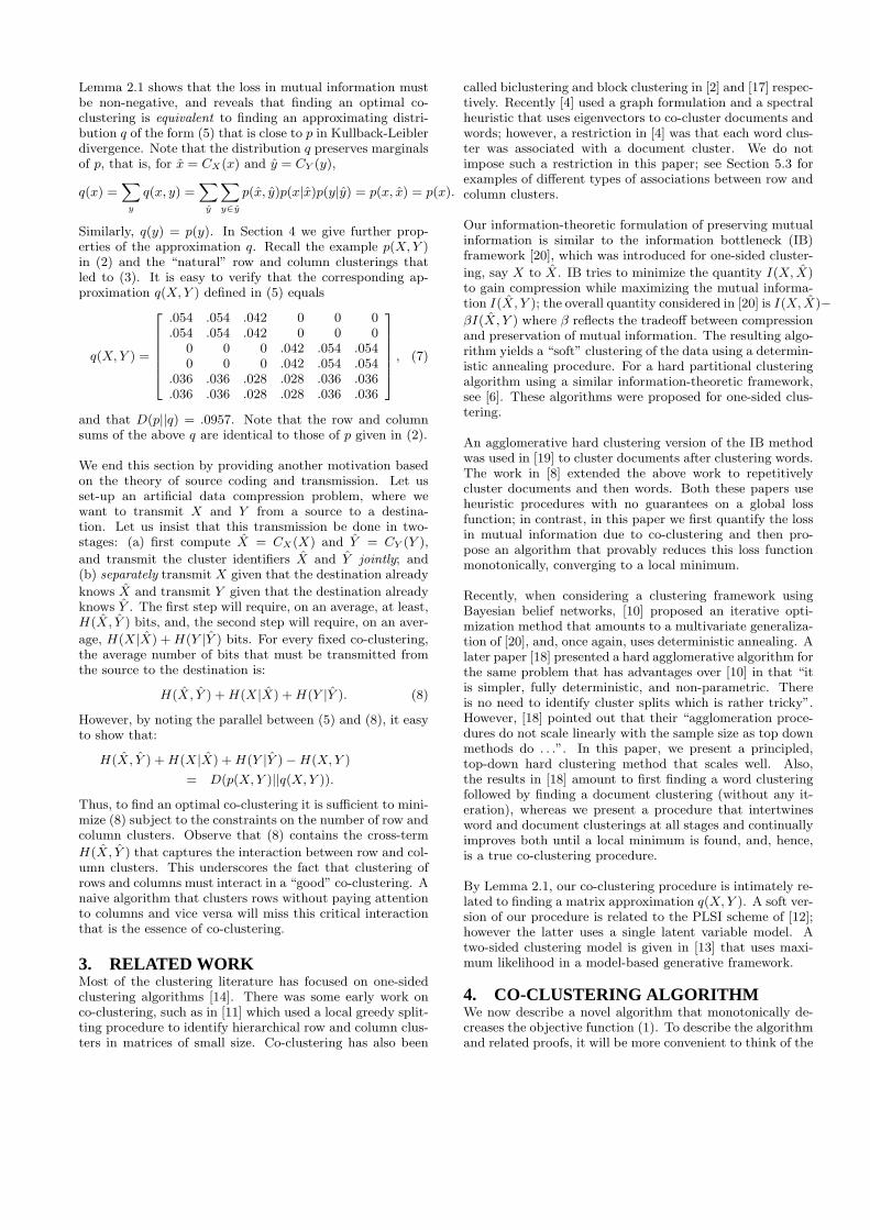
Lemma 2.1 shows that the loss in mutual information mustbe non-negative, and reveals that finding an optimal co-clustering is equivalent to finding an approximating distri-bution q of the form (5) that is close to p in Kullback-Leiblerdivergence. Note that the distribution q preserves marginalsof p, that is, for x = CX(x) and y = CY (y),
q(x) =X
y
q(x, y) =X
y
Xy∈y
p(x, y)p(x|x)p(y|y) = p(x, x) = p(x).
Similarly, q(y) = p(y). In Section 4 we give further prop-erties of the approximation q. Recall the example p(X, Y )in (2) and the “natural” row and column clusterings thatled to (3). It is easy to verify that the corresponding ap-proximation q(X, Y ) defined in (5) equals
q(X, Y ) =
2666664.054 .054 .042 0 0 0.054 .054 .042 0 0 0
0 0 0 .042 .054 .0540 0 0 .042 .054 .054
.036 .036 .028 .028 .036 .036
.036 .036 .028 .028 .036 .036
3777775 , (7)
and that D(p||q) = .0957. Note that the row and columnsums of the above q are identical to those of p given in (2).
We end this section by providing another motivation basedon the theory of source coding and transmission. Let usset-up an artificial data compression problem, where wewant to transmit X and Y from a source to a destina-tion. Let us insist that this transmission be done in two-stages: (a) first compute X = CX(X) and Y = CY (Y ),
and transmit the cluster identifiers X and Y jointly; and(b) separately transmit X given that the destination already
knows X and transmit Y given that the destination alreadyknows Y . The first step will require, on an average, at least,H(X, Y ) bits, and, the second step will require, on an aver-
age, H(X|X) + H(Y |Y ) bits. For every fixed co-clustering,the average number of bits that must be transmitted fromthe source to the destination is:
H(X, Y ) + H(X|X) + H(Y |Y ). (8)
However, by noting the parallel between (5) and (8), it easyto show that:
H(X, Y ) + H(X|X) + H(Y |Y )−H(X, Y )
= D(p(X, Y )||q(X, Y )).
Thus, to find an optimal co-clustering it is sufficient to mini-mize (8) subject to the constraints on the number of row andcolumn clusters. Observe that (8) contains the cross-term
H(X, Y ) that captures the interaction between row and col-umn clusters. This underscores the fact that clustering ofrows and columns must interact in a “good” co-clustering. Anaive algorithm that clusters rows without paying attentionto columns and vice versa will miss this critical interactionthat is the essence of co-clustering.
3. RELATED WORKMost of the clustering literature has focused on one-sidedclustering algorithms [14]. There was some early work onco-clustering, such as in [11] which used a local greedy split-ting procedure to identify hierarchical row and column clus-ters in matrices of small size. Co-clustering has also been
called biclustering and block clustering in [2] and [17] respec-tively. Recently [4] used a graph formulation and a spectralheuristic that uses eigenvectors to co-cluster documents andwords; however, a restriction in [4] was that each word clus-ter was associated with a document cluster. We do notimpose such a restriction in this paper; see Section 5.3 forexamples of different types of associations between row andcolumn clusters.
Our information-theoretic formulation of preserving mutualinformation is similar to the information bottleneck (IB)framework [20], which was introduced for one-sided cluster-
ing, say X to X. IB tries to minimize the quantity I(X, X)to gain compression while maximizing the mutual informa-tion I(X, Y ); the overall quantity considered in [20] is I(X, X)−βI(X, Y ) where β reflects the tradeoff between compressionand preservation of mutual information. The resulting algo-rithm yields a “soft” clustering of the data using a determin-istic annealing procedure. For a hard partitional clusteringalgorithm using a similar information-theoretic framework,see [6]. These algorithms were proposed for one-sided clus-tering.
An agglomerative hard clustering version of the IB methodwas used in [19] to cluster documents after clustering words.The work in [8] extended the above work to repetitivelycluster documents and then words. Both these papers useheuristic procedures with no guarantees on a global lossfunction; in contrast, in this paper we first quantify the lossin mutual information due to co-clustering and then pro-pose an algorithm that provably reduces this loss functionmonotonically, converging to a local minimum.
Recently, when considering a clustering framework usingBayesian belief networks, [10] proposed an iterative opti-mization method that amounts to a multivariate generaliza-tion of [20], and, once again, uses deterministic annealing. Alater paper [18] presented a hard agglomerative algorithm forthe same problem that has advantages over [10] in that “itis simpler, fully deterministic, and non-parametric. Thereis no need to identify cluster splits which is rather tricky”.However, [18] pointed out that their “agglomeration proce-dures do not scale linearly with the sample size as top downmethods do . . .”. In this paper, we present a principled,top-down hard clustering method that scales well. Also,the results in [18] amount to first finding a word clusteringfollowed by finding a document clustering (without any it-eration), whereas we present a procedure that intertwinesword and document clusterings at all stages and continuallyimproves both until a local minimum is found, and, hence,is a true co-clustering procedure.
By Lemma 2.1, our co-clustering procedure is intimately re-lated to finding a matrix approximation q(X, Y ). A soft ver-sion of our procedure is related to the PLSI scheme of [12];however the latter uses a single latent variable model. Atwo-sided clustering model is given in [13] that uses maxi-mum likelihood in a model-based generative framework.
4. CO-CLUSTERING ALGORITHMWe now describe a novel algorithm that monotonically de-creases the objective function (1). To describe the algorithmand related proofs, it will be more convenient to think of the

joint distribution of X, Y, X, and Y . Let p(X, Y, X, Y ) de-note this distribution. Observe that we can write:
p(x, y, x, y) = p(x, y)p(x, y|x, y). (9)
By Lemma 2.1, for the purpose of co-clustering, we willseek an approximation to p(X, Y, X, Y ) using a distribution
q(X, Y, X, Y ) of the form:
q(x, y, x, y) = p(x, y)p(x|x)p(y|y). (10)
The reader may want to compare (5) and (10): observethat the latter is defined for all combinations of x, y, x,and y. Note that in (10) if x 6= CX(x) or y 6= CY (y)then q(x, y, x, y) is zero. We will think of p(X, Y ) as a
two-dimensional marginal of p(X, Y, X, Y ) and q(X, Y ) as
a two-dimensional marginal of q(X, Y, X, Y ). Intuitively, by
(9) and (10), within the co-cluster denoted by X = x and
Y = y, we seek to approximate p(X, Y |X = x, Y = y) by
a distribution of the form p(X|X = x)p(Y |Y = y). Thefollowing proposition (which we state without proof) estab-lishes that there is no harm in adopting such a formulation.
Proposition 4.1. For every fixed “hard” co-clustering,
D(p(X, Y )||q(X, Y )) = D(p(X, Y, X, Y )||q(X, Y, X, Y )).
We first establish a few simple, but useful equalities thathighlight properties of q desirable in approximating p.
Proposition 4.2. For a distribution q of the form (10),the following marginals and conditionals are preserved:
q(x, y) = p(x, y), q(x, x) = p(x, x) & q(y, y) = p(y, y). (11)
Thus,
p(x) = q(x), p(y) = q(y), p(x) = q(x), p(y) = q(y), (12)
p(x|x) = q(x|x), p(y|y) = q(y|y), (13)
p(y|x) = q(y|x), p(x|y) = q(x|y) (14)
∀x, y, x, and y. Further, if y = CY (y) and x = CX(x), then
q(y|x) = q(y|y)q(y|x), (15)
q(x, y, x, y) = p(x)q(y|x), (16)
and, symmetrically,
q(x|y) = q(x|x)q(x|y), (17)
q(x, y, x, y) = p(y)q(x|y).
Proof. The equalities of the marginals in (11) are simpleto show and will not be proved here for brevity. Equalities(12), (13), and (14) easily follow from (11). Equation (15)follows from
q(y|x) = q(y, y|x) =q(y, y, x)
q(x)= q(y|y, x)q(y|x) = q(y|y)q(y|x).
Equation (16) follows from
q(x, y, x, y) = p(x, y)p(x|x)p(y|y)
= p(x)p(x|x)p(y|x)p(y|y)
= p(x, x)p(y|x)p(y|y)
= p(x)q(y|x)q(y|y)
= p(x)q(y|x),
where the last equality follows from (15). tu
Interestingly, q(X, Y ) also enjoys a maximum entropy prop-erty and it can be verified that H(p(X, Y )) ≤ H(q(X, Y ))for any input p(X, Y ).
Lemma 2.1 quantified the loss in mutual information uponco-clustering as the KL-divergence of p(X, Y ) to q(X, Y ).Next, we use the above proposition to prove a lemma thatexpresses the loss in mutual information in two revealingways. This lemma will lead to a “natural” algorithm.
Lemma 4.1. The loss in mutual information can be ex-pressed as (i) a weighted sum of the relative entropies be-tween row distributions p(Y |x) and “row-lumped” distribu-tions q(Y |x), or as (ii) a weighted sum of the relative en-tropies between column distributions p(X|y) and “column-lumped” distributions q(X|y), that is,
D(p(X, Y, X, Y )||q(X, Y, X, Y ))
=X
x
Xx:CX (x)=x
p(x)D(p(Y |x)||q(Y |x)),
D(p(X, Y, X, Y )||q(X, Y, X, Y ))
=X
y
Xy:CY (y)=y
p(y)D(p(X|y)||q(X|y)).
Proof. We show the first equality, the second is similar.
D(p(X, Y, X, Y )||q(X, Y, X, Y ))
=Xx,y
Xx:CX (x)=x,y:CY (y)=y
p(x, y, x, y) logp(x, y, x, y)
q(x, y, x, y)
(a)=
Xx,y
Xx:CX (x)=x,y:CY (y)=y
p(x)p(y|x) logp(x)p(y|x)
p(x)q(y|x)
=X
x
Xx:CX (x)=x
p(x)X
y
p(y|x) logp(y|x)
q(y|x),
where (a) follows from (16) and since p(x, y, x, y) = p(x, y) =p(x)p(y|x) when y = CY (y), x = CX(x). tu
The significance of Lemma 4.1 is that it allows us to expressthe objective function solely in terms of the row-clustering,or in terms of the column-clustering. Furthermore, it allowsus to define the distribution q(Y |x) as a “row-cluster proto-type”, and similarly, the distribution q(X|y) as a “column-cluster prototype”. With this intuition, we now present theco-clustering algorithm in Figure 1. The algorithm works
as follows. It starts with an initial co-clustering (C(0)X , C
(0)Y )
and iteratively refines it to obtain a sequence of co-clusterings:
(C(1)X , C
(1)Y ), (C
(2)X , C
(2)Y ), . . .. Associated with a generic co-
clustering (C(t)X , C
(t)Y ) in the sequence, the distributions p(t)
and q(t) are given by: p(t)(x, y, x, y) = p(t)(x, y)p(t)(x, y|x, y)
and q(t)(x, y, x, y) = p(t)(x, y)p(t)(x|x)p(t)(y|y). Observe that
while as a function of four variables, p(t)(x, y, x, y) depends
upon the iteration index t, the marginal p(t)(x, y) is, in fact,independent of t. Hence, we will write p(x), p(y), p(x|y),
p(y|x), and p(x, y), respectively, instead of p(t)(x), p(t)(y),
p(t)(x|y), p(t)(y|x), and p(t)(x, y).
Algorithm Co Clustering(p,k,`,C†X ,C†
Y )
Input: The joint probability distribution p(X, Y ), k the desirednumber of row clusters, and ` the desired number of columnclusters.
Output: The partition functions C†X and C†
Y .
1. Initialization: Set t = 0. Start with some initial partition
functions C(0)X and C
(0)Y . Compute
q(0)(X, Y ), q(0)(X|X), q(0)(Y |Y )
and the distributions q(0)(Y |x), 1 ≤ x ≤ k using (18).
2. Compute row clusters: For each row x, find its new clusterindex as
C(t+1)X (x) = argminx D
“p(Y |x)||q(t)(Y |x)
”,
resolving ties arbitrarily. Let C(t+1)Y = C
(t)Y .
3. Compute distributions
q(t+1)(X, Y ), q(t+1)(X|X), q(t+1)(Y |Y )
and the distributions q(t+1)(X|y), 1 ≤ y ≤ ` using (19).
4. Compute column clusters: For each column y, find its newcluster index as
C(t+2)Y (y) = argminy D
“p(X|y)||q(t+1)(X|y)
”,
resolving ties arbitrarily. Let C(t+2)X = C
(t+1)X .
5. Compute distributions
q(t+2)(X, Y ), q(t+2)(X|X), q(t+2)(Y |Y )
and the distributions q(t+2)(Y |x), 1 ≤ x ≤ k using (18).
6. Stop and return C†X = C
(t+2)X and C†
Y = C(t+2)Y
if the change in objective function value, that is,D(p(X, Y )||q(t)(X, Y )) − D(p(X, Y )||q(t+2)(X, Y )), is“small” (say 10−3); Else set t = t + 2 and go to step 2.
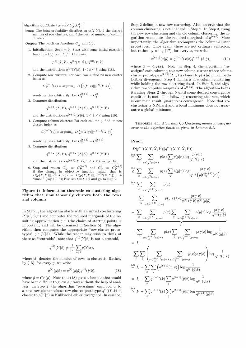
Figure 1: Information theoretic co-clustering algo-rithm that simultaneously clusters both the rowsand columns
In Step 1, the algorithm starts with an initial co-clustering
(C(0)X , C
(0)Y ) and computes the required marginals of the re-
sulting approximation q(0) (the choice of starting points isimportant, and will be discussed in Section 5). The algo-rithm then computes the appropriate “row-cluster proto-types” q(0)(Y |x). While the reader may wish to think of
these as “centroids”, note that q(0)(Y |x) is not a centroid,
q(0)(Y |x) 6= 1
|x|Xx∈x
p(Y |x),
where |x| denotes the number of rows in cluster x. Rather,by (15), for every y, we write
q(t)(y|x) = q(t)(y|y)q(t)(y|x), (18)
where y = CY (y). Note that (18) gives a formula that wouldhave been difficult to guess a priori without the help of anal-ysis. In Step 2, the algorithm “re-assigns” each row x toa new row-cluster whose row-cluster prototype q(t)(Y |x) isclosest to p(Y |x) in Kullback-Leibler divergence. In essence,
Step 2 defines a new row-clustering. Also, observe that thecolumn clustering is not changed in Step 2. In Step 3, usingthe new row-clustering and the old column clustering, the al-gorithm recomputes the required marginals of q(t+1). Moreimportantly, the algorithm recomputes the column-clusterprototypes. Once again, these are not ordinary centroids,but rather by using (17), for every x, we write
q(t+1)(x|y) = q(t+1)(x|x)q(t+1)(x|y), (19)
where x = CX(x). Now, in Step 4, the algorithm “re-assigns” each column y to a new column-cluster whose column-cluster prototype q(t+1)(X|y) is closest to p(X|y) in Kullback-Leibler divergence. Step 4 defines a new column-clusteringwhile holding the row-clustering fixed. In Step 5, the algo-rithm re-computes marginals of q(t+2). The algorithm keepsiterating Steps 2 through 5 until some desired convergencecondition is met. The following reassuring theorem, whichis our main result, guarantees convergence. Note that co-clustering is NP-hard and a local minimum does not guar-antee a global minimum.
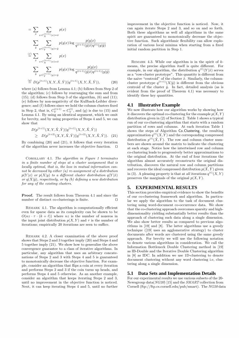
Theorem 4.1. Algorithm Co Clustering monotonically de-creases the objective function given in Lemma 2.1.
Proof.
D(p(t)(X, Y, X, Y )||q(t)(X, Y, X, Y ))
(a)=
Xx
Xx:C
(t)X
(x)=x
p(x)X
y
p(y|x) logp(y|x)
q(t)(y|x)
(b)
≥X
x
Xx:C
(t)X
(x)=x
p(x)X
y
p(y|x) logp(y|x)
q(t)“y|C(t+1)
X (x)”
(c)=
Xx
Xx:C
(t+1)X
(x)=x
p(x)
Xy
Xy:C
(t+1)Y
(y)=y
p(y|x) logp(y|x)
q(t) (y|x) q(t)(y|y)
=X
x
Xx:C
(t+1)X
(x)=x
p(x)X
y
Xy:C
(t+1)Y
(y)=y
p(y|x) logp(y|x)
q(t)(y|y)| {z }I1
+X
x
Xx:C
(t+1)X
(x)=x
p(x)X
y
Xy:C
(t+1)Y
(y)=y
p(y|x) log1
q(t)(y|x)
= I1 +
Xx
Xy
0B@ Xx:C
(t+1)X
(x)=x
Xy:C
(t+1)Y
(y)=y
p(x)p(y|x)
1CA log1
q(t)(y|x)
(d)= I1 +
Xx
Xy
“q(t+1)(x, y)
”log
1
q(t)(y|x)
= I1 +X
x
q(t+1)(x)X
y
q(t+1)(y|x) log1
q(t)(y|x)
(e)
≥ I1 +X
x
q(t+1)(x)X
y
q(t+1)(y|x) log1
q(t+1)(y|x)
=X
x
Xx:C
(t+1)X
(x)=x
p(x)
Xy
Xy:C
(t+1)Y
(y)=y
p(y|x) logp(y|x)
q(t+1)(y|x)q(t)(y|y)
(f)=
Xx
Xx:C
(t+1)X
(x)=x
p(x)
Xy
Xy:C
(t+1)Y
(y)=y
p(y|x) logp(y|x)
q(t+1)(y|x)q(t+1)(y|y)
(g)= D(p(t+1)(X, Y, X, Y )||q(t+1)(X, Y, X, Y )), (20)
where (a) follows from Lemma 4.1; (b) follows from Step 2 ofthe algorithm; (c) follows by rearranging the sum and from(15); (d) follows from Step 3 of the algorithm, (6) and (11);(e) follows by non-negativity of the Kullback-Leibler diver-gence; and (f) follows since we hold the column clusters fixed
in Step 2, that is, C(t+1)Y = C
(t)Y , and (g) is due to (15) and
Lemma 4.1. By using an identical argument, which we omitfor brevity, and by using properties of Steps 4 and 5, we canshow that
D(p(t+1)(X, Y, X, Y )||q(t+1)(X, Y, X, Y ))
≥ D(p(t+2)(X, Y, X, Y )||q(t+2)(X, Y, X, Y )). (21)
By combining (20) and (21), it follows that every iterationof the algorithm never increases the objective function. tu
Corollary 4.1. The algorithm in Figure 1 terminatesin a finite number of steps at a cluster assignment that islocally optimal, that is, the loss in mutual information can-not be decreased by either (a) re-assignment of a distributionp(Y |x) or p(X|y) to a different cluster distribution q(Y |x)or q(X|y), respectively, or by (b) defining a new distributionfor any of the existing clusters.
Proof. The result follows from Theorem 4.1 and since thenumber of distinct co-clusterings is finite. tu
Remark 4.1. The algorithm is computationally efficienteven for sparse data as its complexity can be shown to beO(nz · τ · (k + `)) where nz is the number of nozeros inthe input joint distribution p(X, Y ) and τ is the number ofiterations; empirically 20 iterations are seen to suffice.
Remark 4.2. A closer examination of the above proofshows that Steps 2 and 3 together imply (20) and Steps 4 and5 together imply (21). We show how to generalize the aboveconvergence guarantee to a class of iterative algorithms. Inparticular, any algorithm that uses an arbitrary concate-nations of Steps 2 and 3 with Steps 4 and 5 is guaranteedto monotonically decrease the objective function. For exam-ple, consider an algorithm that flips a coin at every iterationand performs Steps 2 and 3 if the coin turns up heads, andperforms Steps 4 and 5 otherwise. As an another example,consider an algorithm that keeps iterating Steps 2 and 3,until no improvement in the objective function is noticed.Next, it can keep iterating Steps 4 and 5, until no further
improvement in the objective function is noticed. Now, itcan again iterate Steps 2 and 3, and so on and so forth.Both these algorithms as well all algorithms in the samespirit are guaranteed to monotonically decrease the objec-tive function. Such algorithmic flexibility can allow explo-ration of various local minima when starting from a fixedinitial random partition in Step 1.
Remark 4.3. While our algorithm is in the spirit of k-means, the precise algorithm itself is quite different. Forexample, in our algorithm, the distribution q(t)(Y |x) servesas a “row-cluster prototype”. This quantity is different fromthe naive “centroid” of the cluster x. Similarly, the column-cluster prototype q(t+1)(X|y) is different from the obviouscentroid of the cluster y. In fact, detailed analysis (as isevident from the proof of Theorem 4.1) was necessary toidentify these key quantities.
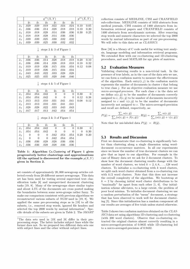
4.1 Illustrative ExampleWe now illustrate how our algorithm works by showing howit discovers the optimal co-clustering for the example p(X, Y )distribution given in (2) of Section 2. Table 1 shows a typicalrun of our co-clustering algorithm that starts with a randompartition of rows and columns. At each iteration Table 1shows the steps of Algorithm Co Clustering, the resultingapproximation q(t)(X, Y ) and the corresponding compressed
distribution p(t)(X, Y ). The row and column cluster num-bers are shown around the matrix to indicate the clusteringat each stage. Notice how the intertwined row and columnco-clustering leads to progressively better approximations tothe original distribution. At the end of four iterations thealgorithm almost accurately reconstructs the original dis-tribution, discovers the natural row and column partitionsand recovers the ideal compressed distribution p(X, Y ) given
in (3). A pleasing property is that at all iterations q(t)(X, Y )preserves the marginals of the original p(X, Y ).
5. EXPERIMENTAL RESULTSThis section provides empirical evidence to show the benefitsof our co-clustering framework and algorithm. In particu-lar we apply the algorithm to the task of document clus-tering using word-document co-occurrence data. We showthat the co-clustering approach overcomes sparsity and high-dimensionality yielding substantially better results than theapproach of clustering such data along a single dimension.We also show better results as compared to previous algo-rithms in [19] and [8]. The latter algorithms use a greedytechnique ([19] uses an agglomerative strategy) to clusterdocuments after words are clustered using the same greedyapproach. For brevity we will use the following notationto denote various algorithms in consideration. We call theInformation Bottleneck Double Clustering method in [19]as IB-Double and the Iterative Double Clustering algorithmin [8] as IDC. In addition we use 1D-clustering to denotedocument clustering without any word clustering i.e, clus-tering along a single dimension.
5.1 Data Sets and Implementation DetailsFor our experimental results we use various subsets of the 20-Newsgroup data(NG20) [15] and the SMART collection fromCornell (ftp://ftp.cs.cornell.edu/pub/smart). The NG20 data
q(t)(X, Y ) p(t)(X, Y )y1 y1 y2 y1 y2 y2
x3 .029 .029 .019 .022 .024 .024 0.10 0.05x1 .036 .036 .014 .028 .018 .018 0.10 0.20x2 .018 .018 .028 .014 .036 .036 0.30 0.25x2 .018 .018 .028 .014 .036 .036x3 .039 .039 .025 .030 .032 .032x3 .039 .039 .025 .030 .032 .032
↓ steps 2 & 3 of Figure 1
y1 y1 y2 y1 y2 y2
x1 .036 .036 .014 .028 .018 .018 0.20 0.10x1 .036 .036 .014 .028 .018 .018 0.18 0.32x2 .019 .019 .026 .015 .034 .034 0.12 0.08x2 .019 .019 .026 .015 .034 .034x3 .043 .043 .022 .033 .028 .028x2 .025 .025 .035 .020 .046 .046
↓ steps 4 & 5 of Figure 1
y1 y1 y1 y2 y2 y2
x1 .054 .054 .042 0 0 0 0.30 0x1 .054 .054 .042 0 0 0 0.12 0.38x2 .013 .013 .010 .031 .041 .041 0.08 0.12x2 .013 .013 .010 .031 .041 .041x3 .028 .028 .022 .033 .043 .043x2 .017 .017 .013 .042 .054 .054
↓ steps 2 & 3 of Figure 1
y1 y1 y1 y2 y2 y2
x1 .054 .054 .042 0 0 0 0.30 0x1 .054 .054 .042 0 0 0 0 0.30x2 0 0 0 .042 .054 .054 0.20 0.20x2 0 0 0 .042 .054 .054x3 .036 .036 .028 .028 .036 .036x3 .036 .036 .028 .028 .036 .036
Table 1: Algorithm Co Clustering of Figure 1 givesprogressively better clusterings and approximationstill the optimal is discovered for the example p(X, Y )given in Section 2.
set consists of approximately 20, 000 newsgroup articles col-lected evenly from 20 different usenet newsgroups. This dataset has been used for testing several supervised text clas-sification tasks [6] and unsupervised document clusteringtasks [19, 8]. Many of the newsgroups share similar topicsand about 4.5% of the documents are cross posted makingthe boundaries between some news-groups rather fuzzy. Tomake our comparison consistent with previous algorithms wereconstructed various subsets of NG20 used in [19, 8]. Weapplied the same pre-processing steps as in [19] to all thesubsets, i.e., removed stop words, ignored file headers andselected the top 2000 words by mutual information1. Spe-cific details of the subsets are given in Table 2. The SMART
1The data sets used in [19] and [8] differ in their pre-processing steps. The latter includes subject lines while theformer does not. So we prepared two different data sets onewith subject lines and the other without subject lines.
collection consists of MEDLINE, CISI and CRANFIELDsub-collections. MEDLINE consists of 1033 abstracts frommedical journals, CISI consists of 1460 abstracts from in-formation retrieval papers and CRANFIELD consists of1400 abstracts from aerodynamic systems. After removingstop words and numeric characters we selected the top 2000words by mutual information as part of our pre-processing.We will refer to this data set as CLASSIC3.
Bow [16] is a library of C code useful for writing text analy-sis, language modeling and information retrieval programs.We extended Bow with our co-clustering and 1D-clusteringprocedures, and used MATLAB for spy plots of matrices.
5.2 Evaluation MeasuresValidating clustering results is a non-trivial task. In thepresence of true labels, as in the case of the data sets we use,we can form a confusion matrix to measure the effectivenessof the algorithm. Each entry(i, j) in the confusion matrixrepresents the number of documents in cluster i that belongto true class j. For an objective evaluation measure we usemicro-averaged-precision. For each class c in the data setwe define α(c, y) to be the number of documents correctlyassigned to c, β(c, y) to be number of documents incorrectlyassigned to c and γ(c, y) to be the number of documentsincorrectly not assigned to c. The micro-averaged-precisionand recall are defined, respectively, as:
P (y) =
Pc α(c, y)P
c(α(c, y) + β(c, y)), R(y) =
Pc α(c, y)P
c(α(c, y) + γ(c, y)).
Note that for uni-labeled data P (y) = R(y).
5.3 Results and DiscussionFirst we demonstrate that co-clustering is significantly bet-ter than clustering along a single dimension using word-document co-occurrence matrices. In all our experimentssince we know the number of true document clusters we cangive that as input to our algorithm. For example in thecase of Binary data set we ask for 2 document clusters. Toshow how the document clustering results change with thenumber of word clusters, we tried k = 2, 4, 8, . . . , 128 wordclusters. To initialize a co-clustering with k word clusters,we split each word cluster obtained from a co-clustering runwith k/2 word clusters. Note that this does not increasethe overall complexity of the algorithm. We bootstrap atk = 2 by choosing initial word cluster distributions to be“maximally” far apart from each other [1, 6]. Our initial-ization scheme alleviates, to a large extent, the problem ofpoor local minima. To initialize document clustering we usea random perturbation of the “mean” document, a strategythat has been observed to work well for document cluster-ing [5]. Since this initialization has a random component allour results are averages of five trials unless stated otherwise.
Table 3 shows two confusion matrices obtained on the CLAS-SIC3 data set using algorithms 1D-clustering and co-clustering(with 200 word clusters). Observe that co-clustering ex-tracted the original clusters almost correctly resulting in amicro-averaged-precision of 0.9835 while 1D-clustering ledto a micro-averaged-precision of 0.9432.
Dataset Newsgroups included #documents Totalper group documents
Binary & Binary subject talk.politics.mideast, talk.politics.misc 250 500Multi5 & Multi5 subject comp.graphics, rec.motorcycles, rec.sports.baseball,
sci.space, talk.politics.mideast 100 500Multi10 & Multi10 subject alt.atheism, comp.sys.mac.hardware, misc.forsale,
rec.autos,rec.sport.hockey, sci.crypt, sci.electronics,sci.med, sci.space, talk.politics.gun 50 500
Table 2: Datasets: Each dataset contains documents randomly sampled from newsgroups in the NG20 corpus.
Co-clustering 1D-clustering992 4 8 944 9 9840 1452 7 71 1431 51 4 1387 18 20 1297
Table 3: Co-clustering accurately recovers originalclusters in the CLASSIC3 data set.
Binary Binary subjectCo-clustering 1D-clustering Co-clustering 1D-clustering244 4 178 104 241 11 179 946 246 72 146 9 239 71 156
Table 4: Co-clustering obtains better clustering re-sults compared to one dimensional document clus-tering on Binary and Binary subject data sets
Table 4 shows confusion matrices obtained by co-clusteringand 1D-clustering on the more “confusable” Binary and Bi-nary subject data sets. While co-clustering achieves 0.98and 0.96 micro-averaged precision on these data sets respec-tively, 1D-clustering yielded only 0.67 and 0.648.
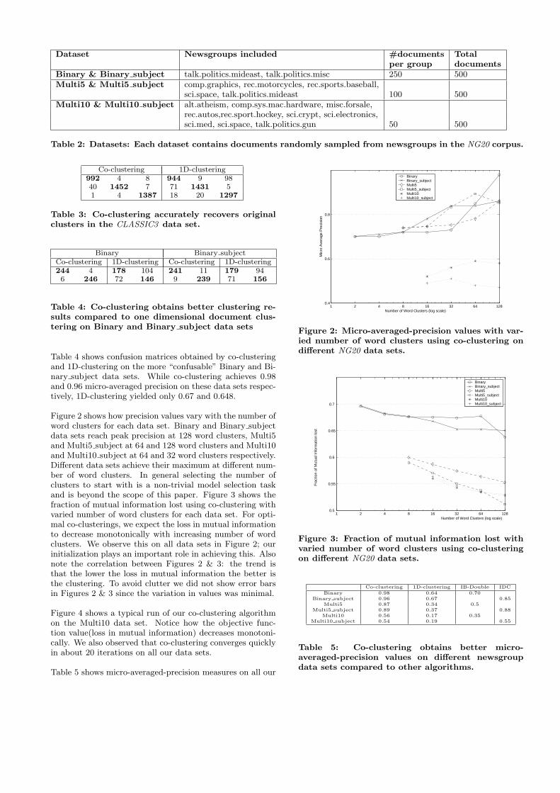
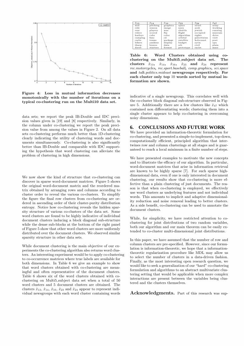
Figure 2 shows how precision values vary with the number ofword clusters for each data set. Binary and Binary subjectdata sets reach peak precision at 128 word clusters, Multi5and Multi5 subject at 64 and 128 word clusters and Multi10and Multi10 subject at 64 and 32 word clusters respectively.Different data sets achieve their maximum at different num-ber of word clusters. In general selecting the number ofclusters to start with is a non-trivial model selection taskand is beyond the scope of this paper. Figure 3 shows thefraction of mutual information lost using co-clustering withvaried number of word clusters for each data set. For opti-mal co-clusterings, we expect the loss in mutual informationto decrease monotonically with increasing number of wordclusters. We observe this on all data sets in Figure 2; ourinitialization plays an important role in achieving this. Alsonote the correlation between Figures 2 & 3: the trend isthat the lower the loss in mutual information the better isthe clustering. To avoid clutter we did not show error barsin Figures 2 & 3 since the variation in values was minimal.
Figure 4 shows a typical run of our co-clustering algorithmon the Multi10 data set. Notice how the objective func-tion value(loss in mutual information) decreases monotoni-cally. We also observed that co-clustering converges quicklyin about 20 iterations on all our data sets.
Table 5 shows micro-averaged-precision measures on all our
1 2 4 8 16 32 64 1280.4
0.6
0.8
Number of Word Clusters (log scale)
Mic
ro A
vera
ge P
reci
sion
BinaryBinary_subjectMulti5Multi5_subjectMulti10Multi10_subject
Figure 2: Micro-averaged-precision values with var-ied number of word clusters using co-clustering ondifferent NG20 data sets.
1 2 4 8 16 32 64 1280.5
0.55
0.6
0.65
0.7
Number of Word Clusters (log scale)
Fra
ctio
n of
Mut
ual I
nfor
mat
ion
lost
BinaryBinary_subjectMulti5Multi5_subjectMulti10Multi10_subject
Figure 3: Fraction of mutual information lost withvaried number of word clusters using co-clusteringon different NG20 data sets.
Co-clustering 1D-clustering IB-Double IDCBinary 0.98 0.64 0.70
Binary subject 0.96 0.67 0.85Multi5 0.87 0.34 0.5
Multi5 subject 0.89 0.37 0.88Multi10 0.56 0.17 0.35
Multi10 subject 0.54 0.19 0.55
Table 5: Co-clustering obtains better micro-averaged-precision values on different newsgroupdata sets compared to other algorithms.
0 2 4 6 8 10 12 14 162.7
2.75
2.8
2.85
Number of Iterations
Obj
ectiv
e_va
lue(
Loss
in M
utua
l Inf
orm
atio
n)
multi10
Figure 4: Loss in mutual information decreasesmonotonically with the number of iterations on atypical co-clustering run on the Multi10 data set.
data sets; we report the peak IB-Double and IDC preci-sion values given in [19] and [8] respectively. Similarly, inthe column under co-clustering we report the peak preci-sion value from among the values in Figure 2. On all datasets co-clustering performs much better than 1D-clusteringclearly indicating the utility of clustering words and doc-uments simultaneously. Co-clustering is also significantlybetter than IB-Double and comparable with IDC support-ing the hypothesis that word clustering can alleviate theproblem of clustering in high dimensions.
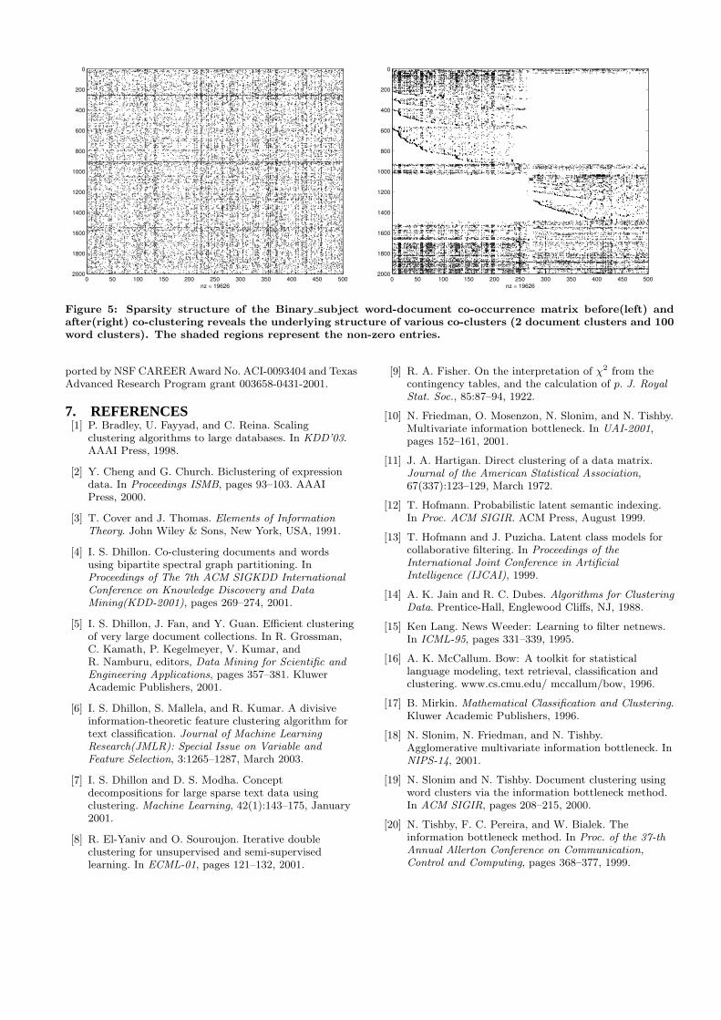
We now show the kind of structure that co-clustering candiscover in sparse word-document matrices. Figure 5 showsthe original word-document matrix and the reordered ma-trix obtained by arranging rows and columns according tocluster order to reveal the various co-clusters. To simplifythe figure the final row clusters from co-clustering are or-dered in ascending order of their cluster-purity distributionentropy. Notice how co-clustering reveals the hidden spar-sity structure of various co-clusters of the data set. Someword clusters are found to be highly indicative of individualdocument clusters inducing a block diagonal sub-structurewhile the dense sub-blocks at the bottom of the right panelof Figure 5 show that other word clusters are more uniformlydistributed over the document clusters. We observed similarsparsity structure in other data sets.
While document clustering is the main objective of our ex-periments the co-clustering algorithm also returns word clus-ters. An interesting experiment would be to apply co-clusteringto co-occurrence matrices where true labels are available forboth dimensions. In Table 6 we give an example to showthat word clusters obtained with co-clustering are mean-ingful and often representative of the document clusters.Table 6 shows six of the word clusters obtained with co-clustering on Multi5 subject data set when a total of 50word clusters and 5 document clusters are obtained. Theclusters x13, x14, x16, x23 and x24 appear to represent indi-vidual newsgroups with each word cluster containing words
x13 x14 x16 x23 x24 x47dod pitching graphics space israel armyride season image nasa arab workingrear players mac shuttle jewish runningriders scored ftp flight occupied museumharleys cubs color algorithm rights drivecamping fans cd orbital palestinian visitcarbs teams package satellite holocaust postbikers yankees display budget syria cputharp braves data srb civil plaindavet starters format prototype racist mass
Table 6: Word Clusters obtained using co-clustering on the Multi5 subject data set. Theclusters x13, x14, x16, x23 and x24 representrec.motorcycles, rec.sport.baseball, comp.graphics, sci.spaceand talk.politics.mideast newsgroups respectively. Foreach cluster only top 10 words sorted by mutual in-formation are shown.
indicative of a single newsgroup. This correlates well withthe co-cluster block diagonal sub-structure observed in Fig-ure 5. Additionally there are a few clusters like x47 whichcontained non differentiating words; clustering them into asingle cluster appears to help co-clustering in overcomingnoisy dimensions.
6. CONCLUSIONS AND FUTURE WORKWe have provided an information-theoretic formulation forco-clustering, and presented a simple-to-implement, top-down,computationally efficient, principled algorithm that inter-twines row and column clusterings at all stages and is guar-anteed to reach a local minimum in a finite number of steps.
We have presented examples to motivate the new conceptsand to illustrate the efficacy of our algorithm. In particular,word-document matrices that arise in information retrievalare known to be highly sparse [7]. For such sparse high-dimensional data, even if one is only interested in documentclustering, our results show that co-clustering is more ef-fective than a plain clustering of just documents. The rea-son is that when co-clustering is employed, we effectivelyuse word clusters as underlying features and not individualwords. This amounts to implicit and adaptive dimensional-ity reduction and noise removal leading to better clusters.As a side benefit, co-clustering can be used to annotate thedocument clusters.
While, for simplicity, we have restricted attention to co-clustering for joint distributions of two random variables,both our algorithm and our main theorem can be easily ex-tended to co-cluster multi-dimensional joint distributions.
In this paper, we have assumed that the number of row andcolumn clusters are pre-specified. However, since our formu-lation is information-theoretic, we hope that a information-theoretic regularization procedure like MDL may allow usto select the number of clusters in a data-driven fashion.Finally, as the most interesting open research question, wewould like to seek a generalization of our “hard” co-clusteringformulation and algorithms to an abstract multivariate clus-tering setting that would be applicable when more complexinteractions are present between the variables being clus-tered and the clusters themselves.
Acknowledgments. Part of this research was sup-
0 50 100 150 200 250 300 350 400 450 500
0
200
400
600
800
1000
1200
1400
1600
1800
2000
nz = 196260 50 100 150 200 250 300 350 400 450 500
0
200
400
600
800
1000
1200
1400
1600
1800
2000
nz = 19626
Figure 5: Sparsity structure of the Binary subject word-document co-occurrence matrix before(left) andafter(right) co-clustering reveals the underlying structure of various co-clusters (2 document clusters and 100word clusters). The shaded regions represent the non-zero entries.
ported by NSF CAREER Award No. ACI-0093404 and TexasAdvanced Research Program grant 003658-0431-2001.
7. REFERENCES[1] P. Bradley, U. Fayyad, and C. Reina. Scaling
clustering algorithms to large databases. In KDD’03.AAAI Press, 1998.
[2] Y. Cheng and G. Church. Biclustering of expressiondata. In Proceedings ISMB, pages 93–103. AAAIPress, 2000.
[3] T. Cover and J. Thomas. Elements of InformationTheory. John Wiley & Sons, New York, USA, 1991.
[4] I. S. Dhillon. Co-clustering documents and wordsusing bipartite spectral graph partitioning. InProceedings of The 7th ACM SIGKDD InternationalConference on Knowledge Discovery and DataMining(KDD-2001), pages 269–274, 2001.
[5] I. S. Dhillon, J. Fan, and Y. Guan. Efficient clusteringof very large document collections. In R. Grossman,C. Kamath, P. Kegelmeyer, V. Kumar, andR. Namburu, editors, Data Mining for Scientific andEngineering Applications, pages 357–381. KluwerAcademic Publishers, 2001.
[6] I. S. Dhillon, S. Mallela, and R. Kumar. A divisiveinformation-theoretic feature clustering algorithm fortext classification. Journal of Machine LearningResearch(JMLR): Special Issue on Variable andFeature Selection, 3:1265–1287, March 2003.
[7] I. S. Dhillon and D. S. Modha. Conceptdecompositions for large sparse text data usingclustering. Machine Learning, 42(1):143–175, January2001.
[8] R. El-Yaniv and O. Souroujon. Iterative doubleclustering for unsupervised and semi-supervisedlearning. In ECML-01, pages 121–132, 2001.
[9] R. A. Fisher. On the interpretation of χ2 from thecontingency tables, and the calculation of p. J. RoyalStat. Soc., 85:87–94, 1922.
[10] N. Friedman, O. Mosenzon, N. Slonim, and N. Tishby.Multivariate information bottleneck. In UAI-2001,pages 152–161, 2001.
[11] J. A. Hartigan. Direct clustering of a data matrix.Journal of the American Statistical Association,67(337):123–129, March 1972.
[12] T. Hofmann. Probabilistic latent semantic indexing.In Proc. ACM SIGIR. ACM Press, August 1999.
[13] T. Hofmann and J. Puzicha. Latent class models forcollaborative filtering. In Proceedings of theInternational Joint Conference in ArtificialIntelligence (IJCAI), 1999.
[14] A. K. Jain and R. C. Dubes. Algorithms for ClusteringData. Prentice-Hall, Englewood Cliffs, NJ, 1988.
[15] Ken Lang. News Weeder: Learning to filter netnews.In ICML-95, pages 331–339, 1995.
[16] A. K. McCallum. Bow: A toolkit for statisticallanguage modeling, text retrieval, classification andclustering. www.cs.cmu.edu/ mccallum/bow, 1996.
[17] B. Mirkin. Mathematical Classification and Clustering.Kluwer Academic Publishers, 1996.
[18] N. Slonim, N. Friedman, and N. Tishby.Agglomerative multivariate information bottleneck. InNIPS-14, 2001.
[19] N. Slonim and N. Tishby. Document clustering usingword clusters via the information bottleneck method.In ACM SIGIR, pages 208–215, 2000.
[20] N. Tishby, F. C. Pereira, and W. Bialek. Theinformation bottleneck method. In Proc. of the 37-thAnnual Allerton Conference on Communication,Control and Computing, pages 368–377, 1999.