Information Support for Groundwater Management in the Wisconsin Central Sands, 2013-2015

A Report to the Wisconsin Department of Natural Resources

George J. Kraft David J. Mechenich

Jessica Haucke

Center for Watershed Science and Education College of Natural Resources

University of Wisconsin – Stevens Point / Extension

August 30, 2016

Information Support for Groundwater Management in the Wisconsin Central Sands, 2013-2015 George J. Kraft David J. Mechenich Jessica Haucke Center for Watershed Science and Education College of Natural Resources University of Wisconsin – Stevens Point / Extension

iii

TABLE OF CONTENTS TABLE OF FIGURES ............................................................................................................................... iii TABLE OF TABLES ................................................................................................................................. iv LIST OF ELECTRONICALLY APPENDED MATERIALS ................................................................ v

1. INTRODUCTION .............................................................................................................................. 1 Objectives of This Effort and Brief Description of How Objectives Were Addressed ................................ 3

2. WEATHER AND HYDROLOGIC CONDITIONS FOR 2014-2015 ............................................ 5 Summary ....................................................................................................................................................... 5 Precipitation .................................................................................................................................................. 5 Drought Index ............................................................................................................................................... 5 Discharges on Reference Streams ................................................................................................................. 6 Groundwater Levels in Areas with Few High Capacity Wells ..................................................................... 6

3. CENTRAL SANDS HIGH CAPACITY WELLS AND GROUNDWATER PUMPING SUMMARY FOR 2013 AND 2014 .......................................................................................................... 11 High Capacity Well Numbers, Uses, and Growth ...................................................................................... 11 2013 and 2014 High Capacity Well Pumping ............................................................................................ 11

4. BASEFLOW DISCHARGES ON SELECT STREAMS – UPDATE ......................................... 15

5. LONG TERM MONITORING WELL WATER LEVELS AND TRENDS – UPDATE .......... 21 Summary ..................................................................................................................................................... 21 Monitoring Wells ........................................................................................................................................ 21 Groundwater Hydrographs .......................................................................................................................... 23 Recent Groundwater Levels and Pumping Drawdowns ............................................................................. 25

6. LAKE LEVEL RECORD AND TRENDS – UPDATE ................................................................ 31 Summary ..................................................................................................................................................... 31 Lake Level Data .......................................................................................................................................... 31 Long Lake – Saxeville Levels ..................................................................................................................... 33 Pumping Effects Update for Four Lakes ..................................................................................................... 34

7. LITTLE PLOVER RIVER 2013-2015 UPDATE .......................................................................... 37 Summary ..................................................................................................................................................... 37 Introduction ................................................................................................................................................. 37 Post 2005 Discharges .................................................................................................................................. 39 Public Rights Flow Failure Rate ................................................................................................................. 39 Pumping in the Little Plover River Vicinity ............................................................................................... 42 Diversions by Municipal and Industrial Pumping ...................................................................................... 45

8. IRRIGATION RATES FOR THE CENTRAL SANDS, 2013-2014 ............................................ 49 Summary ..................................................................................................................................................... 49 Introduction ................................................................................................................................................. 49 Methods ...................................................................................................................................................... 49 Results ......................................................................................................................................................... 51 Conclusions ................................................................................................................................................. 51

LITERATURE CITED ............................................................................................................................ 54

APPENDIX A. Irrigation Rate Estimation by Field for 2013-2014 ................................................... A-1

iii

TABLE OF FIGURES

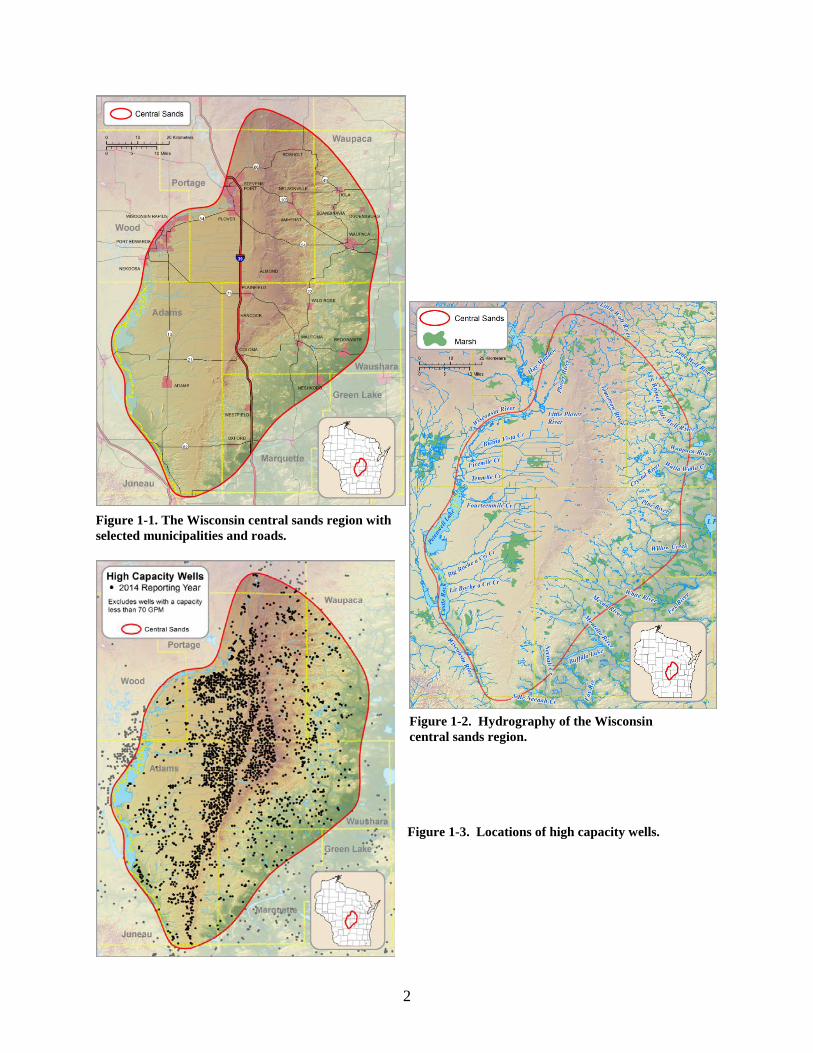
Figure 1-1. The Wisconsin central sands region with selected municipalities and roads. ........................... 2 Figure 1-2. Hydrography of the Wisconsin central sands region. ............................................................... 2 Figure 1-3. Locations of high capacity wells. ............................................................................................. 2 Figure 2-1. Annual precipitation at Stevens Point, Hancock and Wautoma. .............................................. 7 Figure 2-2. Standard departure of annual precipitation and five year average of the standard departure ... 8 Figure 2-3. Palmer Drought Index graph for central Wisconsin ending January 2016 ............................... 9 Figure 2-4. Percentile rank of streamflows by year ending 2015. .............................................................. 9 Figure 2-5. Annual average depth to water in four long term USGS monitoring wells ........................... 10 Figure 3-1. Growth of high capacity wells in the central sands ................................................................ 12 Figure 3-2. High capacity wells in the central sands and their growth since 2000. .................................. 12 Figure 3-3. Total and irrigation high capacity well pumping in the central sands .................................... 14 Figure 4-1. Discharge measurement sites from Kraft et al. 2010 ............................................................. 16 Figure 5-1. Location of eight USGS monitoring wells ............................................................................. 22 Figure 5-2. Annual average water levels in areas of few and many high capacity wells. ......................... 24 Figure 5-3. Measured and expected average annual groundwater elevations at Plover ............................ 27 Figure 5-4. Measured and expected average annual groundwater elevations at Hancock ........................ 28 Figure 5-5. Measured and expected average annual groundwater elevations at Bancroft ........................ 29 Figure 5-6. Measured and expected average annual groundwater elevations at Coloma NW .................. 30 Figure 6-1. Location of lakes with water level data in the project database. ............................................ 31 Figure 6-2. Number of lakes with water level elevations by year ............................................................. 33 Figure 6-3. Hydrograph of Long Lake - Saxeville 1950-2015 ................................................................. 34 Figure 6-4. Declines in water levels at four lakes and the Hancock monitoring well. .............................. 35 Figure 7-1. Little Plover River, its surroundings, and high capacity wells in its vicinity. ........................ 38 Figure 7-2. Baseflow discharges for the Little Plover River ..................................................................... 40 Figure 7-3. Detailed Little Plover baseflows for January 2014 through December 2015. ........................ 41 Figure 7-4. Irrigated land, municipal and industrial high capacity wells, and Del Monte wastewater disposal areas. ............................................................................................................................................. 43 Figure 7-5. Village of Plover total and well-by-well pumping through 2014. .......................................... 44 Figure 7-6. Percentage of Plover pumping from Well 3 ........................................................................... 44 Figure 7-7. Pumping from the Whiting wellfield through December 2014. ............................................. 45 Figure 7-8. Municipal and industrial groundwater pumping diversions from the Little Plover River. .... 47 Figure 8-1. Well and field locations used to estimate irrigation rates ....................................................... 50 Figure 8-2. Median rates for all fields and for four specific crops in central Wisconsin for 2008-2014. . 52 Figure 8-3. 2008-2014 median annual irrigation rates compared with Hancock and Stevens Point summer precipitation. ................................................................................................................................. 52

iv

TABLE OF TABLES

Table 3-1. Central sands high capacity wells ............................................................................................ 11 Table 3-2. Central sands high capacity well pumping .............................................................................. 13 Table 4-1. Discharge measurement sites from Kraft et al. 2010. .............................................................. 17 Table 4-2. Comparison of archived USGS and recent UWSP discharge data (cfs) through 2015. ........... 19 Table 5-1. Useful USGS water level monitoring wells with long term records. ....................................... 22 Table 5-2. Pumping induced water level decline 1999-2008 .................................................................... 23 Table 6-1. Lakes with potentially useful water level information. ............................................................ 32 Table 7-1. Little Plover discharge statistics for the historical record. ....................................................... 38 Table 7-2. Public rights flow failure rates ................................................................................................. 42 Table 7-3. Average annual municipal and industrial diversions ............................................................... 47 Table 8-1. 2013 and 2014 irrigation rates for single and mixed crop fields in central Wisconsin. ........... 53 Table A-1. Irrigation rate estimates by field and crop for 2013. ............................................................. A-1 Table A-2. Irrigation rate estimates by field and crop for 2014. ............................................................. A-4

v

LIST OF ELECTRONICALLY APPENDED MATERIALS

1: Excel file; “Q for Central WI Rivers thru June 2016” 2: Excel file; “Lake Level Data Updated thru 2016” 3. Stream and lake elevation survey (folder) - Survey description - Shapefile 4. Description of past modeling efforts (folder) 5. Refined stream reach segmentation schema (folder)

1

1. INTRODUCTION

This report summarizes data and information gathering for 2013 through 2015 that supports

groundwater management activities in the Wisconsin central sands. The report supplements the previous

work of Clancy et al. (2009) and Kraft et al. (2010, 2012a, 2012b, 2014). These works summarized

important hydrologic literature on the central sands, provided documentation for groundwater flow

models, and statistically analyzed hydrographs for signs of pumping diversions and drawdowns,

concluding that groundwater pumping in the central sands was substantially impacting the region’s water

levels and streamflows, and that stressed water conditions were not explainable by phenomena such as an

unprecedented drought.

The Wisconsin central sands is an extensive (about 2,506 mi2), though loosely-defined, region

characterized by a thick (often > 100 ft) mantle of coarse-grained sediments overlying low permeability

rock, and landforms comprising outwash plains and terminal moraine complexes associated with the

Wisconsin Glaciation. This and the previous works particularly address the area between the headwater

streams of the Fox-Wolf and Central Wisconsin Basins, which contain some 83 lakes larger than 30 acres,

and over 600 miles of headwater streams in close proximity to a great density of high capacity wells

(Figure 1-1 and Figure 1-2).

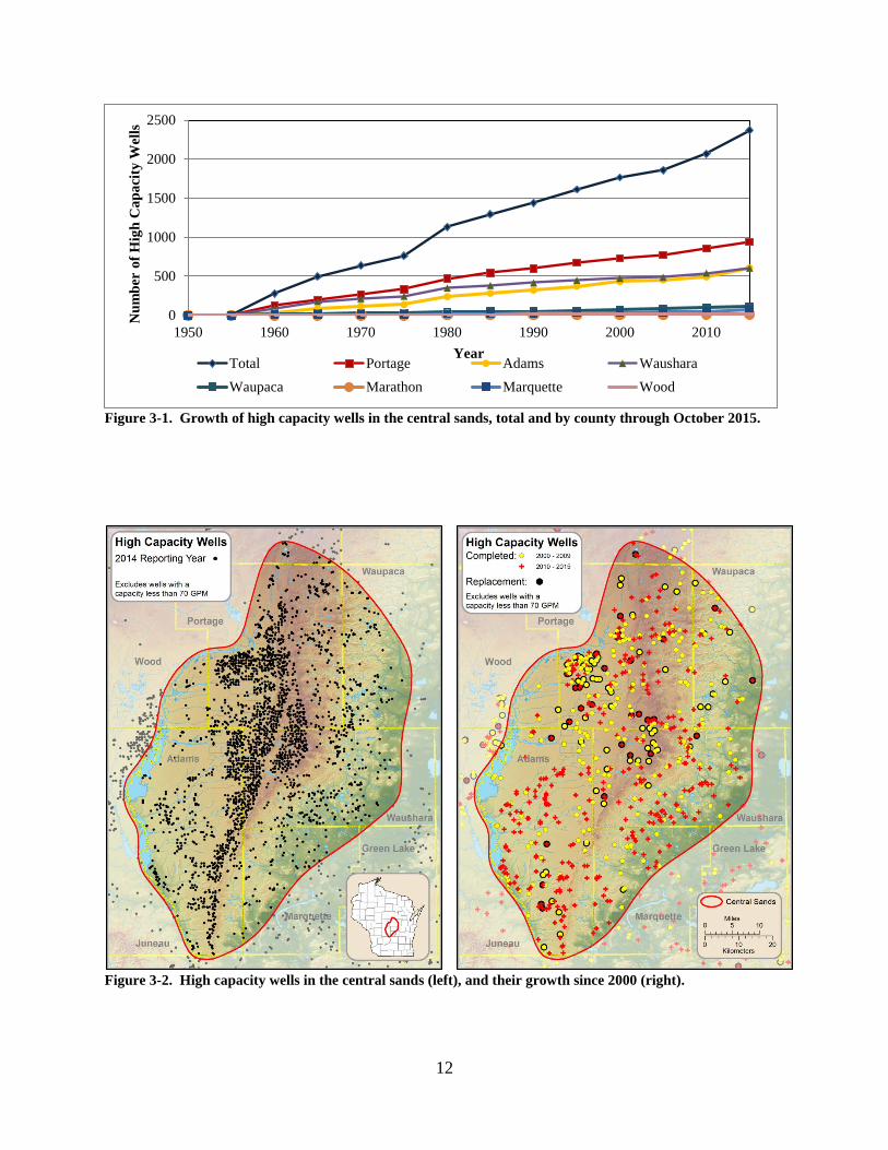
The central sands contains Wisconsin’s greatest density of high capacity wells, about 2,3741 in

the seven counties that this study area overlaps (Figure 1-3). High capacity well pumping in the region

amounted to 28-30% of Wisconsin’s total for 2013-2014; 84-87% was used for agricultural irrigation

(WDNR 2015). Other uses (municipal, industrial) are small and limited geographically, but can have

locally significant surface water impacts (Clancy et al. 2009). Growth in high capacity irrigation well

numbers and pumping has been rapid, minimally managed, and, except for a brief period between the

Richfield Dairy decision in 2014 and Wisconsin Attorney General’s opinion in 2016, with minimal regard

for impacts on lake, stream, and wetland resources.

Lake levels, groundwater levels, and streamflows associated with irrigated portions of the

Wisconsin central sands have been depressed in recent years. For instance, Long Lake near Plainfield,

which in recent times covered 45 acres and had a typical depth of about 10 feet, was near dry to dry in

2005-2009, and even the very large rains in 2010-2011 restored only a few feet of water. Low lake levels

have apparently provoked more frequent winter fish kills on Portage County’s Pickerel Lake. Wolf Lake

County Park in Portage County has had its swimming beach closed due to low water levels for 14

1 High capacity wells for these purposes are defined as wells with a stated maximum pumping capacity of 70 gallons per minute (gpm) or more. Wells with an unknown maximum were also included if the total annual pumping exceeds 365 days, (or 153 days for irrigation wells) of 70 gpm or more.

2

Figure 1-3. Locations of high capacity wells.

Figure 1-2. Hydrography of the Wisconsin central sands region.

Figure 1-1. The Wisconsin central sands region with selected municipalities and roads.

3

years. The Little Plover River, which formerly (1959-1987) discharged at a mean of 10 and a one-day

minimum of 3.9 cubic feet per second (cfs) (Hoover Road gauge), now frequently flows at less than the

former minimum, and was below the Public Rights Flow (WDNR 2009) 37-53% of the time in 2013.

Objectives of This Effort and Brief Description of How Objectives Were Addressed

The goal of this project is to provide monitoring and modeling support for management and policy

processes that address groundwater pumping effects on aquatic resources in the Wisconsin central sands,

with these specific objectives: 1. Measure baseflow discharges on select streams and groundwater levels in select wells; provide data

to USGS and WDNR for archiving.

Baseflow was measured at 32 stream locations (Chapter 4) and groundwater levels were measured at four.

Data have been uploaded to agencies and are provided as electronically appended material. 2. Estimate irrigation rates for crops grown in central Wisconsin for years 2013 and 2014.

Results are provided in Chapter 8. 3. Compile precipitation, groundwater, and lake level data from NOAA, WDNR, County, and USGS

data sources for years 2014 and 2015 and merge with previously compiled data. Use the assembled

data to provide a context for the relative wetness or dryness of the study period.

Results are provided in Chapter 2. 4. Estimate pumping drawdowns for select monitoring wells and lakes for 2014-2015 by statistical

comparisons to reference sites.

Results are provided in Chapters 5 and 6. 5. Run existing groundwater flow models to meet agency and process needs and to explore cause-and-

effect relationships of diminished surface waters to groundwater pumping.

This work occurred irregularly through the life of this two-year project with results passed along to

agency contacts. 6. Collaborate with Department staff in irrigation rate and modeling analyses.

Results are presented in Chapter 8. Other

A stream and lake elevation survey, groundwater modeling documentation, and refined stream reach

segmentation schema are included as electronic files.

5

2. WEATHER AND HYDROLOGIC CONDITIONS FOR 2014-2015

Summary

Precipitation in 2014 and 2015, respectively, was greater than average by 4.0 and 8.8 inches at

Stevens Point, 4.2 and 0.9 inches at Hancock, and 6.8 and 4.1 inches at Wautoma. The Palmer Drought

Index ranged from near normal to unusually moist, and has not fallen below “normal,” or average, since

the end of 2012. Discharges at reference streams were above average, at the 77th-80th percentile, as were

groundwater levels in most areas with few high capacity wells.

Precipitation

2014 and 2015 precipitation

Years 2014 and 2015 were wetter than average, by 4.0 and 8.8 inches at Stevens Point (2014 and

2015 respectively), 4.2 and 0.9 inches at Hancock, and 6.8 and 4.1 inches at Wautoma.

Long term precipitation trends

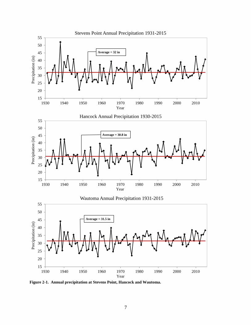
Precipitation amounts for 1930 through 2015 are displayed in Figure 2-1 and Figure 2-2 for

Stevens Point, Hancock, and Wautoma. Stevens Point and Hancock records are virtually complete for the

period, but the Wautoma record needed to be inferred through 2008 using the methods of Serbin and

Kucharik (2009).

Notable in the long term record is a prolonged dry period that prevailed in 1946 through 1964,

when precipitation was less than average by 2.1-2.7 inches/year at the three stations. Hydrographs from

monitoring wells, lakes, and streams during this period often express depressed conditions. Precipitation

since then has generally increased, consistent with wetter conditions that have prevailed over much of the

eastern US, including Wisconsin, since 1970 (Juckem et al. 2008, WICCI 2011). In more recent times,

average precipitation at the three stations was 0.2-2.1 inches above the mean during 2000-2009, and 1.2-

3.6 inches during 2010-2015.

Drought Index

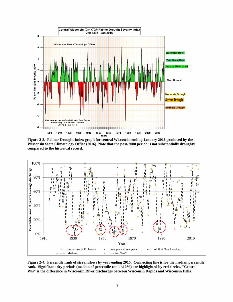
The Palmer Drought Index (Figure 2-3) is an indicator of weather wetness and dryness based on

precipitation and temperature. It is an improvement on precipitation alone as a wet/dry indicator, as it

contains an algorithm that uses temperature as a surrogate for evapotranspiration.

The Palmer Index in 2014 and 2015 ranged from near normal to unusually moist, and has not

fallen below “normal,” or average, since the end of 2012.

6

Discharges on Reference Streams

Long term annual stream discharges provide context for hydrologic conditions. Displayed in

Figure 2-4 are the percentile rank of annual streamflows for four streams that surround the central sands:

the Wolf River at New London (1914-2015), the Embarrass River at Embarrass (1920-2015 with nine

missing years), the Waupaca River at Waupaca (1917-1984 with 20 missing years, plus 2009-2015), and

the Wisconsin River between Wisconsin Dells and Wisconsin Rapids (1935-2015 with eight missing

years). We term the Wisconsin River between Wisconsin Dells and Wisconsin Rapids as the “Wisconsin

River – Central,” obtaining discharge values as the difference between Wisconsin Rapids and Wisconsin

Dells discharges. Wisconsin River – Central replaced the Wisconsin at Wisconsin Dells and at Wisconsin

Rapids in previous reports, which we found to be heavily biased by northern Wisconsin weather. We also

left out Ten Mile Creek at Nekoosa, as it has apparently become irrigation pumping affected.

Each of the stream gauges has limitations when used as a reference for the central sands. The

Wolf River at New London drains a large basin to the northeast and somewhat distant from the central

sands, and hence is subject to differing weather conditions. The Embarrass River at Embarrass is closer

and drains a smaller basin (384 mi2), but is also outside the central sands. The Waupaca River at

Waupaca is in the central sands and does not seem overly affected by irrigation pumping at this time, but

has a sparse record for 1962 through 2009. The Wisconsin River – Central might be confounded by dam

storage and release.

Previously, discharge data from these reference gauges were used to demonstrate significant low

flow periods (defined as percentile ranks of 10% or less, which amounts to about a 10 year return

frequency) during the past ~ 90 years, which include 1931-1934, 1948-1949, 1957-1959, 1964, 1977, and

1988. The 1930s discharges were the smallest on record, and years 1948-1964 mark a long period when

low flows were unusually common (6 of 17 years). In more recent times, years 2000-2004 were about

average, while 2005-2009 were somewhat low. Discharges since have mostly been above average, and

were at the 80th and 77th percentiles in 2014 and 2015.

Groundwater Levels in Areas with Few High Capacity Wells

Four USGS monitoring wells located in areas with relatively few high capacity wells have been

used to provide a context for hydrologic conditions under an assumed small pumping influence (Kraft et

al. 2010, 2012a, 2014). These are Amherst Junction (1958 to 2015 record), Nelsonville (1950 to 1998, 2010 to 2015), Wild Rose (1956 to 1998), and Wautoma (1956 to 2015) (Figure 2-5). The record shows

groundwater levels were at long term lows in the late 1950s and early 1960s, rose through about 1974,

and since have mostly fluctuated cyclically (Kraft et al. 2010, 2012b). Amherst Junction levels were

noticeably low in 2007-2010, but Wautoma levels were not. 2014 and 2015 levels continued to rise and

7

Figure 2-1. Annual precipitation at Stevens Point, Hancock and Wautoma.

15

20

25

30

35

40

45

50

55

1930 1940 1950 1960 1970 1980 1990 2000 2010

Prec

ipita

tion

(in)

Year

Stevens Point Annual Precipitation 1931-2015

15

20

25

30

35

40

45

50

55

1930 1940 1950 1960 1970 1980 1990 2000 2010

Prec

ipita

tion

(in)

Year

Hancock Annual Precipitation 1930-2015

Average = 32 in

Average = 30.8 in

15

20

25

30

35

40

45

50

55

1930 1940 1950 1960 1970 1980 1990 2000 2010

Prec

ipita

tion

(in)

Year

Wautoma Annual Precipitation 1931-2015

Average = 31.5 in

8

Stevens Point

Hancock

Wautoma

Figure 2-2. Standard departure of annual precipitation and five year average of the standard departure for Stevens Point, Hancock, and Wautoma.

-4

-2

0

2

4

1930 1950 1970 1990 2010

Stan

dard

Dep

artu

re

Year

Precipitation Standard Departure1931-2015

-2

-1

0

1

2

1930 1950 1970 1990 2010

Stan

dard

Dep

artu

re

Year

Precipitation Standard Departure 5 Year Average

-4

-2

0

2

4

1930 1950 1970 1990 2010

Stan

dard

Dep

artu

re

Year

Precipitation Standard Departure 1930-2015

-2

-1

0

1

2

1930 1950 1970 1990 2010

Stan

dard

Dep

artu

re

Year

Precipitation Standard Departure 5 Year Average

-2

-1

0

1

2

1930 1950 1970 1990 2010

Stan

dard

Dep

artu

re

Year

Precipitation Standard Departure 5 Year Average

-4

-2

0

2

4

1930 1950 1970 1990 2010

Stan

dard

Dep

artu

re

Year

Precipitation Standard Departure1931-2015

9

Figure 2-3. Palmer Drought Index graph for central Wisconsin ending January 2016 produced by the Wisconsin State Climatology Office (2016). Note that the post-2000 period is not substantially droughty compared to the historical record.

Figure 2-4. Percentile rank of streamflows by year ending 2015. Connecting line is for the median percentile rank. Significant dry periods (median of percentile rank <10%) are highlighted by red circles. "Central Wis" is the difference in Wisconsin River discharges between Wisconsin Rapids and Wisconsin Dells.

0%

20%

40%

60%

80%

100%

1910 1930 1950 1970 1990 2010

Perc

entil

e ra

nk o

f yea

r's a

vera

ge d

isch

arge

YearEmbarrass at Embarass Waupaca at Waupaca Wolf at New LondonMedian Central Wis*

10

Figure 2-5. Annual average depth to water in four long term USGS monitoring wells located in areas with fewer high capacity wells. Water levels were adjusted so that 1969 values were zero for display purposes. were high at Amherst Junction (75th and 79th percentile for 2014 and 2015, respectively), and at

Nelsonville (85th and 86th percentile), but were about average at Wautoma (47th and 64th percentile).

Though the three stations currently producing water level data (Amherst Junction, Nelsonville,

and Wautoma) are in areas with relatively few high capacity wells, they are still somewhat influenced by

pumping. Groundwater flow modeling suggests that pumping may lower water levels at these locations

by 0.4 to 0.76 feet on average (Kraft et al. 2012b). Haucke (2010) found the somewhat low water levels

at Amherst Junction following 2000 could not be explained by precipitation alone, and could be

consistent with a pumping effect. The revived Nelsonville well, which has less pumping influence than

Amherst Junction, may prove to be a better reference location in the future as more data accumulate.

-6

-4

-2

0

2

4

61950 1960 1970 1980 1990 2000 2010

Wat

er D

epth

(ft)

YearAmherst Jct. Nelsonville Wild Rose Wautoma

11

3. CENTRAL SANDS HIGH CAPACITY WELLS AND GROUNDWATER PUMPING SUMMARY FOR 2013 AND 2014

High Capacity Well Numbers, Uses, and Growth

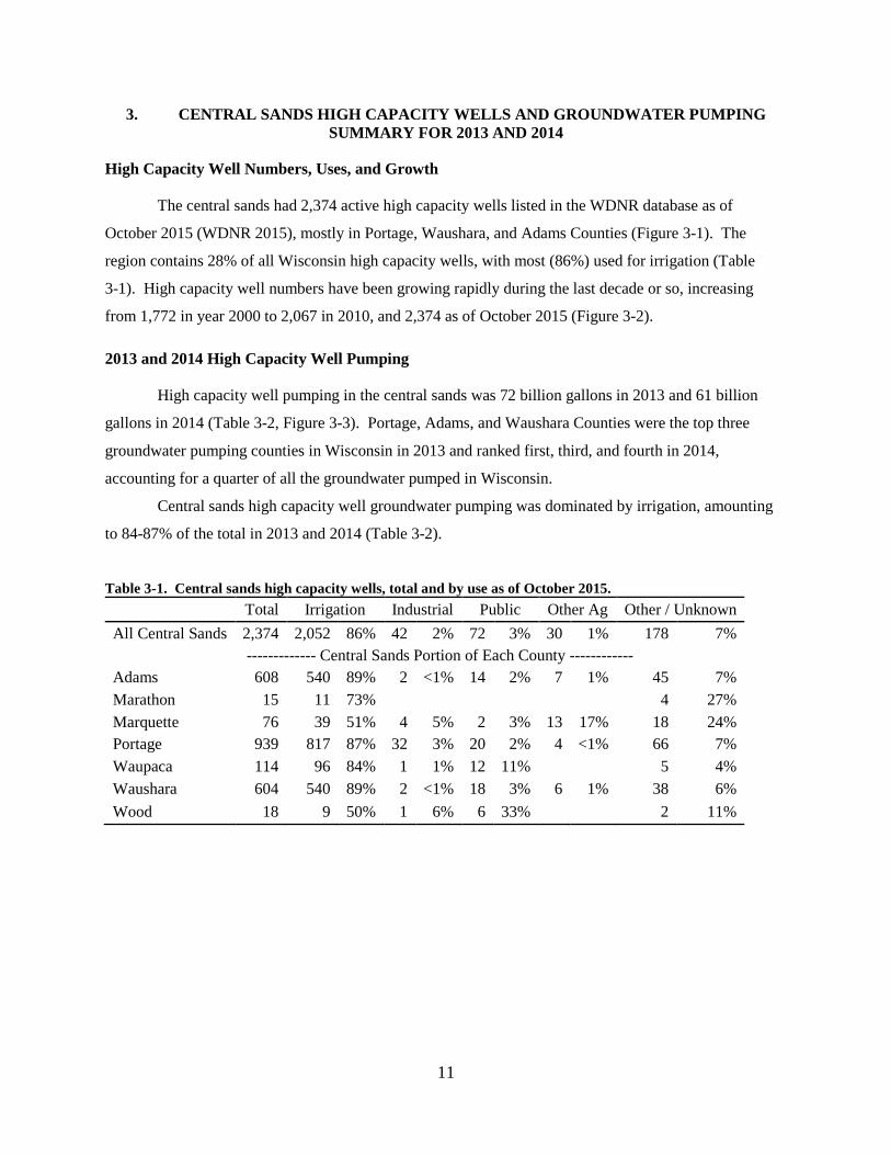
The central sands had 2,374 active high capacity wells listed in the WDNR database as of

October 2015 (WDNR 2015), mostly in Portage, Waushara, and Adams Counties (Figure 3-1). The

region contains 28% of all Wisconsin high capacity wells, with most (86%) used for irrigation (Table

3-1). High capacity well numbers have been growing rapidly during the last decade or so, increasing

from 1,772 in year 2000 to 2,067 in 2010, and 2,374 as of October 2015 (Figure 3-2).

2013 and 2014 High Capacity Well Pumping

High capacity well pumping in the central sands was 72 billion gallons in 2013 and 61 billion

gallons in 2014 (Table 3-2, Figure 3-3). Portage, Adams, and Waushara Counties were the top three

groundwater pumping counties in Wisconsin in 2013 and ranked first, third, and fourth in 2014,

accounting for a quarter of all the groundwater pumped in Wisconsin.

Central sands high capacity well groundwater pumping was dominated by irrigation, amounting

to 84-87% of the total in 2013 and 2014 (Table 3-2).

Table 3-1. Central sands high capacity wells, total and by use as of October 2015. Total Irrigation Industrial Public Other Ag Other / Unknown All Central Sands 2,374 2,052 86% 42 2% 72 3% 30 1% 178 7%

------------- Central Sands Portion of Each County ------------ Adams 608 540 89% 2 <1% 14 2% 7 1% 45 7% Marathon 15 11 73% 4 27% Marquette 76 39 51% 4 5% 2 3% 13 17% 18 24% Portage 939 817 87% 32 3% 20 2% 4 <1% 66 7% Waupaca 114 96 84% 1 1% 12 11% 5 4% Waushara 604 540 89% 2 <1% 18 3% 6 1% 38 6% Wood 18 9 50% 1 6% 6 33% 2 11%

12

Figure 3-1. Growth of high capacity wells in the central sands, total and by county through October 2015.

Figure 3-2. High capacity wells in the central sands (left), and their growth since 2000 (right).

0

500

1000

1500

2000

2500

1950 1960 1970 1980 1990 2000 2010

Num

ber

of H

igh

Cap

acity

Wel

ls

YearTotal Portage Adams WausharaWaupaca Marathon Marquette Wood

13

Table 3-2. Central sands high capacity well pumping, total and by county, for 2013 and 2014, billions of gallons.

2013

Total Irrigation Industrial Public Other Ag Other/ Unknown

All Central Sands 72.08 62.82 87% 2.15 3% 4.63 6% 2.4 3% 0.07 <1%

-------------- Central Sands Portion of Each County -------------

Adams 20.14 19.67 98% 0.02 <1% 0.28 1% 0.14 1% 0.04 <1% Marathon 0.12 0.12 100% 0 0% 0 0% 0 0% 0 0% Marquette 1.98 1.03 52% 0.1 5% 0.001 <1% 0.84 42% 0.001 <1%

Portage 26.84 22.14 82% 2.01 7% 2.64 10% 0.05 0% 0.0017 <1% Waupaca 2.64 1.89 72% 0.024 1% 0.72 27% 0 0% 0 0%

Waushara 19.49 17.87 92% 0.003 <1% 0.21 1% 1.37 7% 0.03 <1% Wood 0.87 0.1 11% 0.001 <1% 0.77 89% 0 0% 0 0%

2014

Total Irrigation Industrial Public Other Ag Other/ Unknown

All Central Sands 61.47 51.88 84% 2.13 3% 5.02 8% 2.42 4% 0.03 <1%

-------------- Central Sands Portion of Each County -------------

Adams 17.94 17.53 98% 0.01 <1% 0.25 1% 0.14 1% 0.01 <1% Marathon 0.06 0.06 100% 0 0% 0 0% 0 0% 0 0% Marquette 1.97 1 51% 0.12 6% 0.001 <1% 0.84 43% 0 0%

Portage 21.12 16.53 78% 1.98 9% 2.56 12% 0.05 <1% 0 0% Waupaca 2.67 1.87 70% 0.01 <1% 0.79 30% 0 0% 0 0%

Waushara 16.36 14.72 90% 0.003 <1% 0.23 1% 1.39 8% 0.02 <1% Wood 1.36 0.17 13% 0 0% 1.19 88% 0 0% 0 0%

14

Figure 3-3. Total and irrigation high capacity well pumping in the central sands, total and by county, 2013 and 2014.

0

20

40

60

80

Bill

ions

of g

allo

ns p

er y

ear

Locale

2013

Total Irrigation

0

10

20

30

40

50

60

70

Bill

ions

of g

allo

ns p

er y

ear

Locale

2014

Total Irrigation

15

4. BASEFLOW DISCHARGES ON SELECT STREAMS – UPDATE

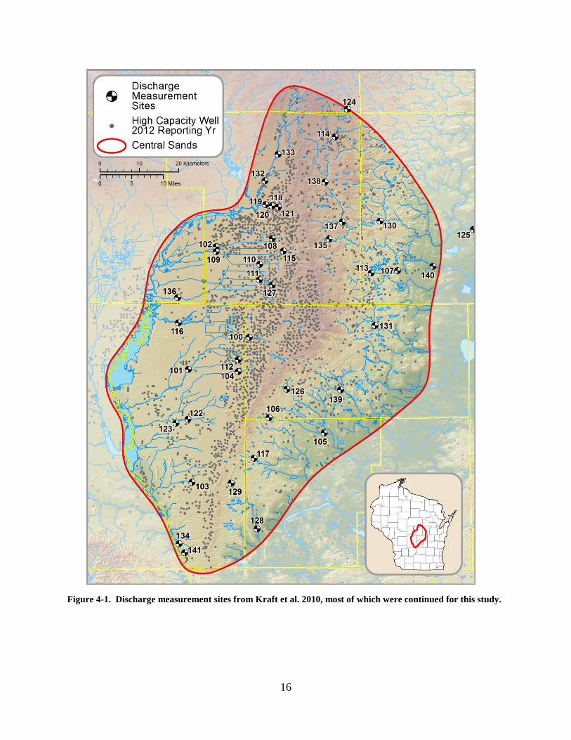
Baseflow discharge measurements continued at 32 of 42 stream locations (Figure 4-1, Table 4-1)

previously measured by Kraft et al. (2010). Discharges were measured monthly through the study period

except in January and April of 2013. Most of the 32 sites had discharge histories that predated Kraft et al.

2010. Thirteen were at or near current and former USGS daily discharge sites, and eight were at USGS

miscellaneous or “spot” sites that had one or more occasional measurements. Thirteen sites, including

eight USGS sites, were gauged as part of the Fox-Wolf project in 2005-2006 (Kraft et al. 2008) (Table

4-1). Data for locations with both UWSP and USGS histories are summarized and compared in Table

4-2. Complete data are included with this report as electronic media in a spreadsheet entitled “Q for

Central WI Rivers thru June 2016.xlsx.” Data collected through June 2016 were sent to USGS to be

archived in their database.

16

Figure 4-1. Discharge measurement sites from Kraft et al. 2010, most of which were continued for this study.

17

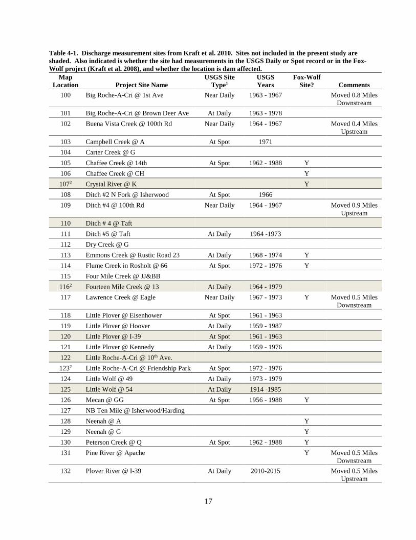
Table 4-1. Discharge measurement sites from Kraft et al. 2010. Sites not included in the present study are shaded. Also indicated is whether the site had measurements in the USGS Daily or Spot record or in the Fox-Wolf project (Kraft et al. 2008), and whether the location is dam affected.

Map Location Project Site Name

USGS Site Type1

USGS Years

Fox-Wolf Site? Comments

100 Big Roche-A-Cri @ 1st Ave Near Daily 1963 - 1967 Moved 0.8 Miles Downstream

101 Big Roche-A-Cri @ Brown Deer Ave At Daily 1963 - 1978 102 Buena Vista Creek @ 100th Rd Near Daily 1964 - 1967 Moved 0.4 Miles

Upstream 103 Campbell Creek @ A At Spot 1971 104 Carter Creek @ G 105 Chaffee Creek @ 14th At Spot 1962 - 1988 Y 106 Chaffee Creek @ CH Y 1072 Crystal River @ K Y 108 Ditch #2 N Fork @ Isherwood At Spot 1966 109 Ditch #4 @ 100th Rd Near Daily 1964 - 1967 Moved 0.9 Miles

Upstream 110 Ditch # 4 @ Taft 111 Ditch #5 @ Taft At Daily 1964 -1973 112 Dry Creek @ G 113 Emmons Creek @ Rustic Road 23 At Daily 1968 - 1974 Y 114 Flume Creek in Rosholt @ 66 At Spot 1972 - 1976 Y 115 Four Mile Creek @ JJ&BB 1162 Fourteen Mile Creek @ 13 At Daily 1964 - 1979 117 Lawrence Creek @ Eagle Near Daily 1967 - 1973 Y Moved 0.5 Miles

Downstream 118 Little Plover @ Eisenhower At Spot 1961 - 1963 119 Little Plover @ Hoover At Daily 1959 - 1987 120 Little Plover @ I-39 At Spot 1961 - 1963 121 Little Plover @ Kennedy At Daily 1959 - 1976 122 Little Roche-A-Cri @ 10th Ave. 1232 Little Roche-A-Cri @ Friendship Park At Spot 1972 - 1976 124 Little Wolf @ 49 At Daily 1973 - 1979 125 Little Wolf @ 54 At Daily 1914 -1985 126 Mecan @ GG At Spot 1956 - 1988 Y 127 NB Ten Mile @ Isherwood/Harding 128 Neenah @ A Y 129 Neenah @ G Y 130 Peterson Creek @ Q At Spot 1962 - 1988 Y 131 Pine River @ Apache Y Moved 0.5 Miles

Downstream 132 Plover River @ I-39 At Daily 2010-2015 Moved 0.5 Miles

Upstream

18

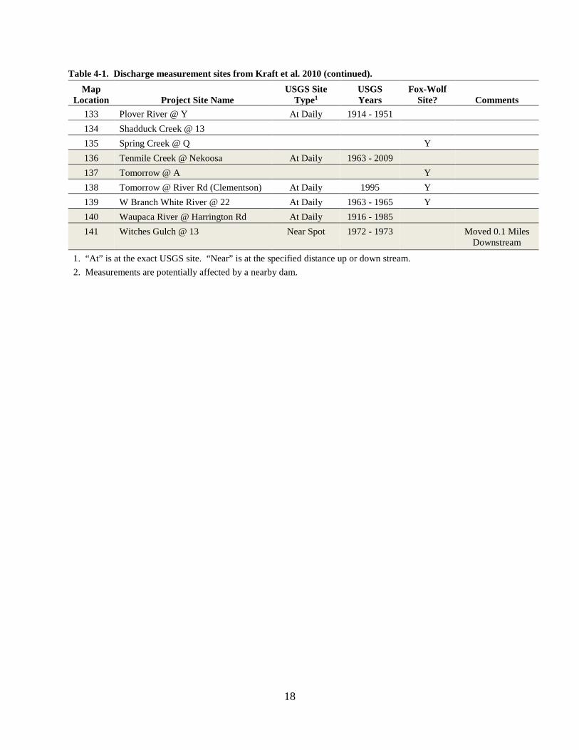
Table 4-1. Discharge measurement sites from Kraft et al. 2010 (continued).

Map Location Project Site Name

USGS Site Type1

USGS Years

Fox-Wolf Site? Comments

133 Plover River @ Y At Daily 1914 - 1951 134 Shadduck Creek @ 13 135 Spring Creek @ Q Y 136 Tenmile Creek @ Nekoosa At Daily 1963 - 2009 137 Tomorrow @ A Y 138 Tomorrow @ River Rd (Clementson) At Daily 1995 Y 139 W Branch White River @ 22 At Daily 1963 - 1965 Y 140 Waupaca River @ Harrington Rd At Daily 1916 - 1985 141 Witches Gulch @ 13 Near Spot 1972 - 1973 Moved 0.1 Miles

Downstream

1. “At” is at the exact USGS site. “Near” is at the specified distance up or down stream. 2. Measurements are potentially affected by a nearby dam.

19

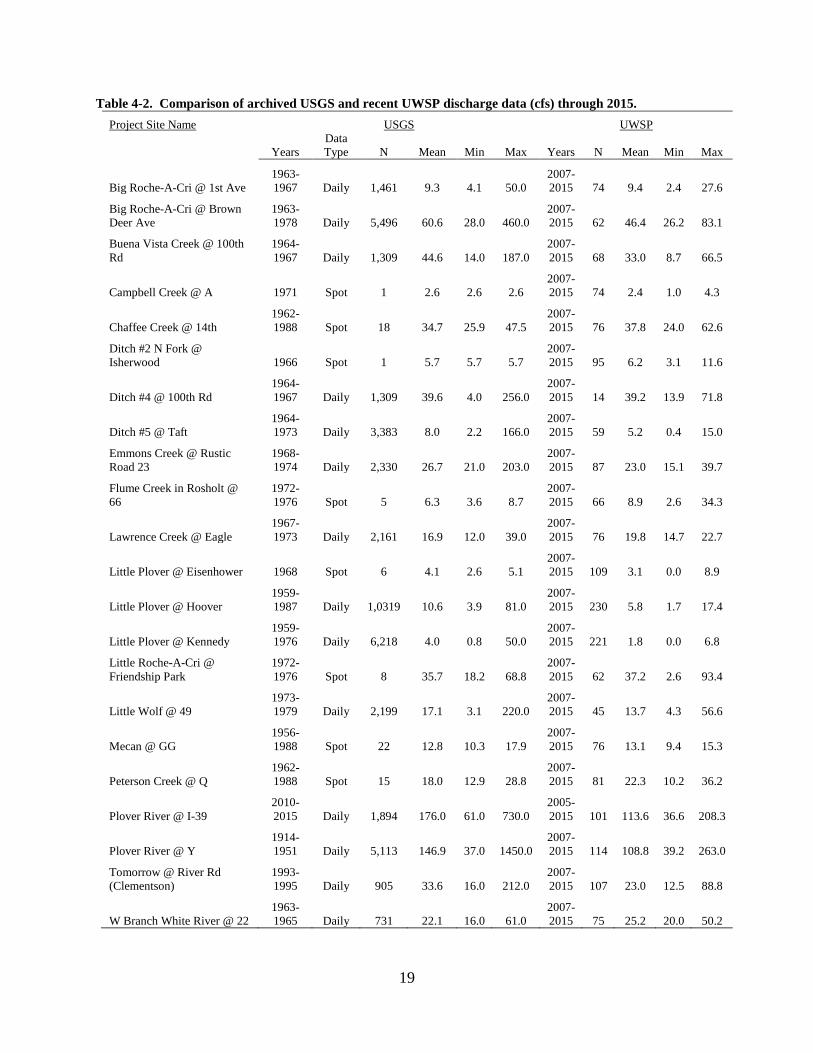
Table 4-2. Comparison of archived USGS and recent UWSP discharge data (cfs) through 2015. Project Site Name USGS UWSP

Years Data Type N Mean Min Max Years N Mean Min Max

Big Roche-A-Cri @ 1st Ave 1963-1967 Daily 1,461 9.3 4.1 50.0

2007-2015 74 9.4 2.4 27.6

Big Roche-A-Cri @ Brown Deer Ave

1963-1978 Daily 5,496 60.6 28.0 460.0

2007-2015 62 46.4 26.2 83.1

Buena Vista Creek @ 100th Rd

1964-1967 Daily 1,309 44.6 14.0 187.0

2007-2015 68 33.0 8.7 66.5

Campbell Creek @ A 1971 Spot 1 2.6 2.6 2.6 2007-2015 74 2.4 1.0 4.3

Chaffee Creek @ 14th 1962-1988 Spot 18 34.7 25.9 47.5

2007-2015 76 37.8 24.0 62.6

Ditch #2 N Fork @ Isherwood 1966 Spot 1 5.7 5.7 5.7

2007-2015 95 6.2 3.1 11.6

Ditch #4 @ 100th Rd 1964-1967 Daily 1,309 39.6 4.0 256.0

2007-2015 14 39.2 13.9 71.8

Ditch #5 @ Taft 1964-1973 Daily 3,383 8.0 2.2 166.0

2007-2015 59 5.2 0.4 15.0

Emmons Creek @ Rustic Road 23

1968-1974 Daily 2,330 26.7 21.0 203.0

2007-2015 87 23.0 15.1 39.7

Flume Creek in Rosholt @ 66

1972-1976 Spot 5 6.3 3.6 8.7

2007-2015 66 8.9 2.6 34.3

Lawrence Creek @ Eagle 1967-1973 Daily 2,161 16.9 12.0 39.0

2007-2015 76 19.8 14.7 22.7

Little Plover @ Eisenhower 1968 Spot 6 4.1 2.6 5.1 2007-2015 109 3.1 0.0 8.9

Little Plover @ Hoover 1959-1987 Daily 1,0319 10.6 3.9 81.0

2007-2015 230 5.8 1.7 17.4

Little Plover @ Kennedy 1959-1976 Daily 6,218 4.0 0.8 50.0

2007-2015 221 1.8 0.0 6.8

Little Roche-A-Cri @ Friendship Park

1972-1976 Spot 8 35.7 18.2 68.8

2007-2015 62 37.2 2.6 93.4

Little Wolf @ 49 1973-1979 Daily 2,199 17.1 3.1 220.0

2007-2015 45 13.7 4.3 56.6

Mecan @ GG 1956-1988 Spot 22 12.8 10.3 17.9

2007-2015 76 13.1 9.4 15.3

Peterson Creek @ Q 1962-1988 Spot 15 18.0 12.9 28.8

2007-2015 81 22.3 10.2 36.2

Plover River @ I-39 2010-2015 Daily 1,894 176.0 61.0 730.0

2005-2015 101 113.6 36.6 208.3

Plover River @ Y 1914-1951 Daily 5,113 146.9 37.0 1450.0

2007-2015 114 108.8 39.2 263.0

Tomorrow @ River Rd (Clementson)

1993-1995 Daily 905 33.6 16.0 212.0

2007-2015 107 23.0 12.5 88.8

W Branch White River @ 22 1963-1965 Daily 731 22.1 16.0 61.0

2007-2015 75 25.2 20.0 50.2

21

5. LONG TERM MONITORING WELL WATER LEVELS AND TRENDS – UPDATE

Summary

The long-term records of eight central sands monitoring wells have proved useful for exploring

groundwater level trends over the last 60 years and for separating the influences of pumping from the

influences of weather. Four of the eight monitoring wells, three of which are still active, are located in

areas with few high capacity wells and are only modestly affected by high capacity well pumping. Their

levels are thus representative of groundwater controlled mostly by weather. Levels in few high capacity

well areas demonstrated record lows during the 1950s and early 1960s, concurrent with the acute drought

that prevailed at the time. Water levels rose from these lows through 1974 and have since fluctuated

cyclically. Levels were somewhat low during 2005-2010 (at the 5th to 23rd percentile of record,

depending on locale), but rebounded sharply following the wet 2010-2011 years and in 2014-2015 were at

the 47th to 91st percentiles of record.

The four monitoring wells located in areas with many high capacity wells are substantially

pumping affected. Their water levels initially paralleled those of few high capacity well areas, but began

an incongruent decline during 1973-1990, depending on locale. Water levels plummeted in 2005-2010 to

lows deeper than the 1950s drought. Recent levels in many high capacity well areas were still at or near

the record lows of the pre-pumping era. Drawdowns in 2013-2014 were estimated at about 4.5 feet at

Plover and Hancock, 0.5 feet at Bancroft, and 2.3 feet at Coloma.

Monitoring Wells

The records of eight monitoring wells in the USGS archives have proved useful (Kraft et al. 2010,

2012a, 2014) for exploring central sands groundwater level trends over the last half-century (Table 5-1,

Figure 5-1). Four of the eight monitoring wells (Amherst Junction, Nelsonville, Wild Rose, and

Wautoma) are in areas with relatively few high capacity wells, and four (Plover1, Hancock, Bancroft, and

Coloma NW) are in areas with many high capacity wells. Here we update the analysis of these records

for 2014-2015.

Water level records suffer several deficiencies. The Wild Rose record terminated in 1994, and

the Nelsonville record lacks observations for 1998-2010. Records are sparse at some locations during

some periods, particularly at Coloma NW. With the reconstruction of the Nelsonville monitoring well

(Kraft et al. 2012a), seven of the eight wells are currently generating data.

1 Three wells have been located at the Plover site with water levels recorded under two different well numbers in the USGS database. Data explored in this study use combined information from these three wells referenced to a common datum, discussed further in Kraft et al. 2010.

22

Table 5-1. Useful USGS water level monitoring wells with long term records.

USGS Station Name Locale or Quadrangle

Well Depth (ft)

First Observation

Last Observation

Number of Observations

PT-24/10E/28-0015* Nelsonville 52.0 8/24/1950 2015+ 1,372+ PT-23/10E/18-0276 Amherst Jct. 17.4 7/2/1958 2015+ 1,740+ PT-23/08E/25-0376** Plover 19.0 12/1/1959 2015+ 1,214+ WS-18/10E/01-0105 Wautoma 14.0 4/18/1956 2015+ 18,974+ WS-19/08E/15-0008 Hancock 18.0 5/1/1951 2015+ 20,479+ PT-21/08E/10-0036 Bancroft 12.0 9/7/1950 2015+ 1,684+ PT-21/07E/31-0059*** Coloma NW 15.3 8/8/1951 2015+ 787+ WS-20/11E/02-0053 Wild Rose 177.0 2/6/1956 5/20/1994 442 * Replaced by 443126089174201 on November 17, 2010. ** Three different monitoring wells have been located at this site, see text. ***Replaced by 441452089433001 in 1995

Figure 5-1. Location of eight USGS monitoring wells with records sufficient for exploring long term water level trends.

23

Groundwater Hydrographs

Updated annual average hydrographs are displayed in Figure 5-2, grouped by location in areas of

few or many high capacity wells. For display purposes, average annual water levels in each well were

zeroed to the well’s 1969 level, with positive values indicating a greater depth to water (water level

decline) compared with 1969, and negative values a shallower depth (water level rise).

The hydrographs demonstrate some common peaks (evident around 1974, 1985, and 1993) and

valleys (1959, 1978, 1990, and 2007) that coincide with wet and dry weather periods (Chapter 2).

Though peaks and valleys coincide, amplitudes and trends differ. Amplitude differences are expected and

are explainable by groundwater hydraulics: groundwater levels near discharge zones are constrained by

the water level of the discharge zone, while groundwater levels far from discharge zones are less

constrained. Thus, groundwater levels at the Coloma NW and Bancroft locations, which are near

groundwater discharge zones, have small amplitudes.

Though water level amplitudes are explainable by the location within the groundwater flow

system, water level trends conform as to whether monitoring wells are in an area of fewer or many high

capacity wells. Levels in areas with fewer high capacity wells were at their record lows during the late

1950s - early 1960s, coincident with a decade that witnessed some years of the smallest precipitation

amounts and stream discharges of the twentieth century (Chapter 2). In contrast, water levels in areas

with many high capacity wells were lower during the modestly dry period of 2005-2010 than the historic

record lows. The declines in areas of many high capacity wells are beyond what is explainable by

weather variability alone and are attributed to a pumping effect (Kraft et al. 2010, 2012a). Water level

decline start date, rate, and average 1999-2008 amount were previously estimated (Table 5-2, Kraft et al.

2010, 2012a, 2012b).

Table 5-2. Pumping induced water level decline 1999-2008, decline rate, and approximate start of decline for monitoring wells in high density irrigated areas (Kraft et al. 2012a, 2012b).

Station Comparison Station(s) Decline (ft) Decline rate (ft y-1) Decline start Plover Amherst Junction 2.1 (3.4)1,* 0.12 1973 Hancock Wautoma 3.2* 0.21 1990 Bancroft Amherst Junction 0.82* 0.062 1984 Bancroft Wautoma 1.2* 0.062 1984 Coloma NW Amherst Junction 0.0 -- -- Coloma NW Wautoma 2.2* -- 1978 * Decline is significant at 0.05 level. 1 Total decline = 3.4 ft; irrigation decline = 2.1 ft

24

Figure 5-2. Annual average water levels in areas of few (top) and many (bottom) high capacity wells. Water levels are zeroed to 1969 water depths for display purposes.

-6

-4

-2

0

2

4

61950 1960 1970 1980 1990 2000 2010

Wat

er D

epth

(ft)

Year

Few High Capacity Wells

Amherst Jct. Nelsonville Wild Rose Wautoma

-6

-4

-2

0

2

4

61950 1960 1970 1980 1990 2000 2010

Wat

er D

epth

(ft)

Year

Many High Capacity Wells

Plover Hancock Bancroft Coloma

25

Recent Groundwater Levels and Pumping Drawdowns

Groundwater levels since 2011 have been mostly steady. Levels in areas of fewer high capacity

well were generally above average, at the 47th to 91st percentile, while those in areas with many high

capacity wells were near or below their historic drought minimums.

Year-by-year pumping declines in pumping affected areas were estimated by subtracting the

actual measured water level from the water level expected in the absence of pumping. Expected water

levels in the absence of pumping were generated using the relationship of water levels in the areas with

many high capacity wells to water levels in one or more wells in areas with few high capacity wells

(“reference” areas) during an early baseline period when pumping effects were assumed small. More

detail on methodology is documented in Kraft et al. (2010, 2012a).

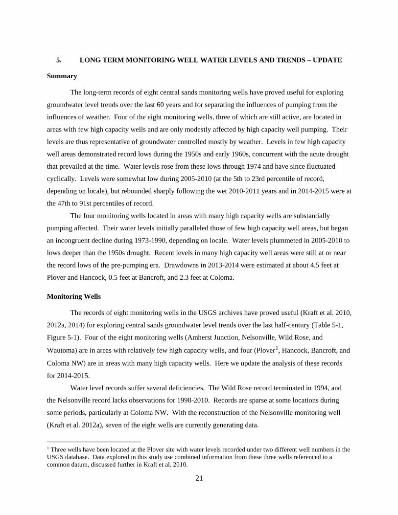
Plover Water levels at the Plover monitoring well have been decreasing since the 1980s (Figure 5-3,

top), and reached a record low in 2007-2008. Pumping drawdowns at Plover were estimated at 4.5 feet

for 2014-2015 (Figure 5-3, bottom).

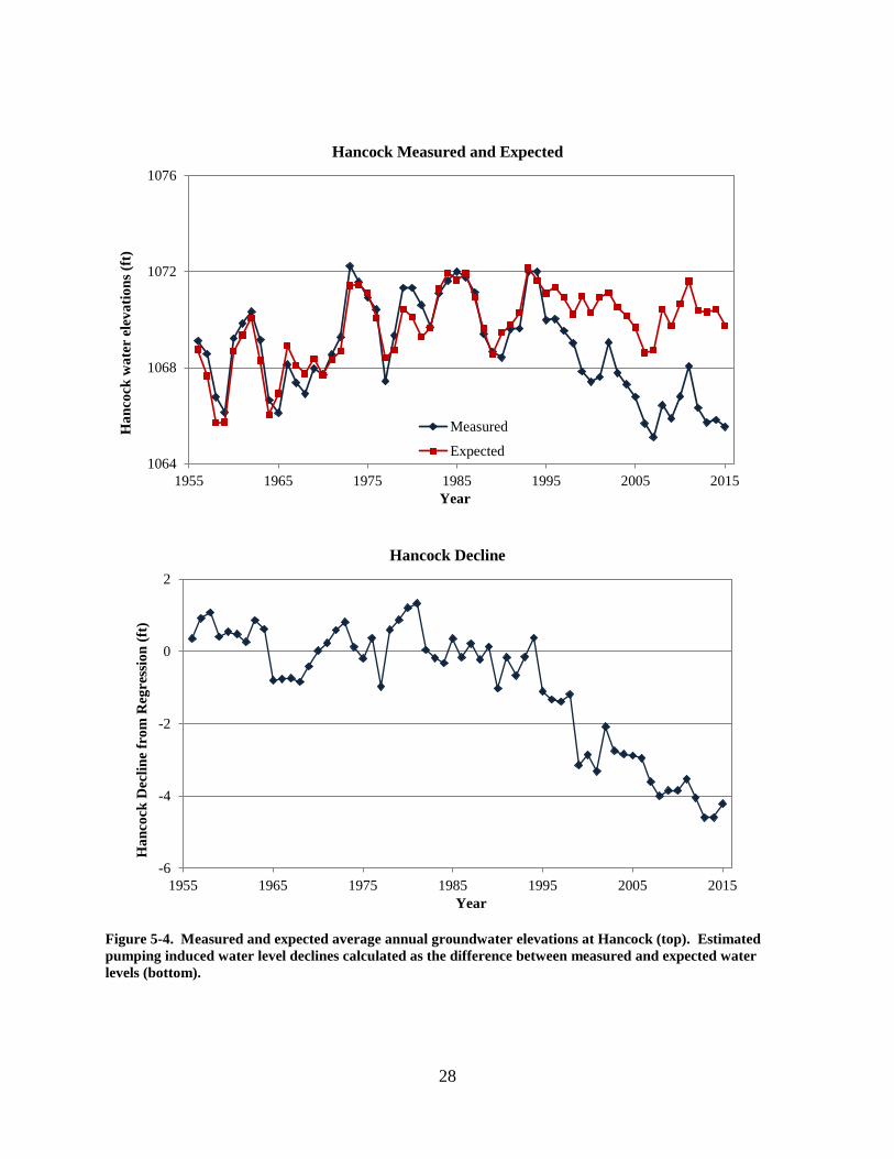
Hancock Water levels at Hancock began a systematic decrease around 1990, and were at record lows

through much of 2006-2009 (Figure 5-4, top). Water levels rebounded several feet in 2010-2011 (again,

presumably in response to large rains), but fell by about 2 feet in 2012-2013. Estimated pumping declines

in 2014-2015 were about 4.4 feet (Figure 5-4 bottom).

Bancroft

Bancroft water levels have been in decline since the mid-1980s and were at record lows during

much of 2003-2007 (Figure 5-5, top). Estimated pumping declines at Bancroft were calculated against

both Wautoma and Amherst Junction, since Bancroft is not particularly nearer to either. The comparison

against Wautoma is likely more appropriate, as the Bancroft early water level record correlates more

closely with Wautoma, and precipitation increase patterns are more similar. Pumping induced declines at

Bancroft have an apparent beginning around 1984, and in 1999-2008 averaged 1.2 feet, Wautoma

reference (Figure 5-5, bottom), or 0.82 feet, Amherst Junction reference. Estimated average pumping

declines in 2014-2015 were 0.34 feet (Wautoma) and 0.55 feet (Amherst Junction).

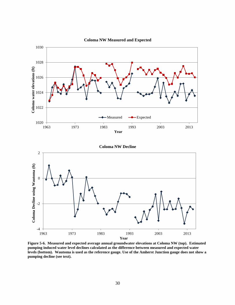
Coloma NW Groundwater levels at Coloma NW have generally been declining since the early 1990s. Levels

were at a low for the 1964-2015 record in 2006, rebounded to near the long term average in 2010-2011,

26

and in 2012-2015 were near the low of the long term record (Figure 5-6, top).

Coloma NW water levels are odd compared with other sites, possibly because of complications

due to its location near a groundwater discharge. The Coloma locale is also distant from both the

Amherst Junction and Wautoma reference wells and not well correlated with either. For this reason, the

methodology used here to estimate the influence of groundwater pumping gives differing estimates

depending on the reference well. The expected water level in absence of pumping and estimated pumping

decline are shown relative to the Wautoma reference well in Figure 5-6 (bottom), which indicates a

maximum pumping decline of 3.6 feet in 2012 and a decline in 2014-2015 of 2.4 feet. Comparisons using

the Amherst Junction reference site indicates a maximum pumping decline of 3.0 feet in 2012 and a

decline in 2014-2015 of 1.7 feet. Haucke (2010), using a statistical method based on precipitation,

estimated a pumping drawdown averaging 0.7 feet at Coloma NW.

27

Plover Measured and Expected

Plover Decline

Figure 5-3. Measured and expected average annual groundwater elevations at Plover (top). Estimated pumping induced water level declines calculated as the difference between measured and expected water levels (bottom).

1076

1080

1084

1088

1958 1968 1978 1988 1998 2008

Plov

er w

ater

ele

vatio

ns (f

t)

Year

Measured

Expected

-6

-4

-2

0

2

4

1958 1968 1978 1988 1998 2008

Plov

er D

eclin

e (f

t)

Year

28

Hancock Measured and Expected

Hancock Decline

Figure 5-4. Measured and expected average annual groundwater elevations at Hancock (top). Estimated pumping induced water level declines calculated as the difference between measured and expected water levels (bottom).

1064

1068

1072

1076

1955 1965 1975 1985 1995 2005 2015

Han

cock

wat

er e

leva

tions

(ft)

Year

Measured

Expected

-6

-4

-2

0

2

1955 1965 1975 1985 1995 2005 2015

Han

cock

Dec

line

from

Reg

ress

ion

(ft)

Year

29

Bancroft Measured and Expected

Bancroft Decline

Figure 5-5. Measured and expected average annual groundwater elevations at Bancroft (top). Estimated pumping induced water level declines calculated as the difference between measured and expected water levels (bottom). Wautoma reference shown, Amherst Junction is similar.

1067

1068

1069

1070

1071

1955 1965 1975 1985 1995 2005 2015

Ban

crof

t wat

er e

leva

tions

(ft)

Year

Measured

Expected

-2

-1

0

1

2

1955 1965 1975 1985 1995 2005 2015

Ban

crof

t Dec

line

Usi

ng W

auto

ma

(ft)

Year

30

Coloma NW Measured and Expected

Coloma NW Decline

Figure 5-6. Measured and expected average annual groundwater elevations at Coloma NW (top). Estimated pumping induced water level declines calculated as the difference between measured and expected water levels (bottom). Wautoma is used as the reference gauge. Use of the Amherst Junction gauge does not show a pumping decline (see text).

1020

1022

1024

1026

1028

1030

1963 1973 1983 1993 2003 2013

Col

oma

wat

er e

leva

tions

(ft)

Year

Measured Expected

-4

-2

0

2

1963 1973 1983 1993 2003 2013

Col

oma

Dec

line

usin

g W

auto

ma

(ft)

Year

31

6. LAKE LEVEL RECORD AND TRENDS – UPDATE

Summary

Lake levels for previously inventoried lakes were downloaded and added to the project’s

database. For the 31 lakes with data, levels were at long-term lows in 2007. Levels increased by an

average 2.6 feet in 2011, presumably due to large rains in 2010-2011. Levels have since declined, by an

average 1.4 feet through 2015. The drawdowns of four lakes previously found to have large and

significant pumping declines were revisited. Estimated drawdowns in the four, which reached 3.3 to 8

feet in 2007-2010, were 1.8 to 5.5 feet in 2015.

Lake Level Data

Kraft et al. (2010) previously identified 39 lakes with potentially useful level records in agency

archives (Figure 6-1). The lake data inventory (Table 6-1) and level data base (Lake Level Data Updated

Figure 6-1. Location of lakes with water level data in the project database.

32

Table 6-1. Lakes with potentially useful water level information.

Lake Name County

Number of Levels

First Lake Level

Last Lake Level

Avg. Years Between Levels

Bean's Lake Waushara 19 7/10/73 8/26/15 2.22 Big Hills Lake (Hills) Waushara 18 9/7/95 8/28/15 1.11 Big Silver Lake Waushara 31 5/14/66 8/26/15 1.59 Big Twin Lake Waushara 21 6/18/75 8/27/15 1.92 Burghs Lake Waushara 26 9/7/73 8/26/15 1.62 Crooked Lake Adams 12 6/14/73 6/20/89 1.34 Curtis Lake Waushara 18 9/12/95 8/24/15 1.11 Deer Lake Waushara 19 7/28/93 8/26/15 1.16 Fenner Lake Adams 8 4/25/74 6/13/85 1.39 Fish Lake Waushara 19 7/10/73 8/24/15 2.22 Gilbert Lake Waushara 36 5/10/62 8/27/15 1.48 Huron Lake Waushara 21 7/3/73 8/24/15 2.01 Irogami Lake Waushara 32 1/1/31 8/26/15 2.65 John's Lake Waushara 19 7/28/93 8/28/15 1.16 Jordan Lake Adams 20 9/8/67 9/6/90 1.15 Kusel Lake Waushara 34 9/30/63 8/28/15 1.53 Lake Lucerne Waushara 30 9/30/63 8/26/15 1.73 Lake Napowan Waushara 22 5/21/85 8/28/15 1.38 Lake Sharon Marquette 72 11/17/84 5/31/94 0.13 Lime Lake Portage 6 10/2/40 11/7/94 9.02 Little Hills Lake Waushara 15 8/3/01 8/26/15 0.94 Little Silver Lake Waushara 19 7/20/93 8/28/15 1.16 Little Twin Lake Waushara 20 5/21/85 8/27/15 1.51 Long Lake Waushara 31 8/16/61 8/24/15 1.74 Long Lake Saxeville1 Waushara 22 11/3/87 8/27/15 1.27 Long Lake Saxeville2 Waushara 84 6/1/47 7/1/09 0.74 Marl Lake Waushara 18 4/1/98 8/24/15 0.97 Norwegian Lake Waushara 20 6/23/75 8/28/15 2.01 Parker Lake Adams 13 5/26/83 9/6/90 0.56 Patrick Lake Adams 9 5/6/77 6/16/86 1.01 Pearl Lake Waushara 19 6/17/75 8/26/15 2.12 Pine Lake Hancock Waushara 23 7/10/73 8/24/15 1.83 Pine Lake (Springwater) Waushara 35 2/8/61 8/27/15 1.56 Pleasant Lake Waushara 29 7/9/64 8/24/15 1.76 Porter's Lake Waushara 14 7/26/02 8/28/15 0.94 Round Lake Waushara 17 4/1/98 8/28/15 1.02 Spring Lake Waushara 26 10/1/63 8/26/15 2.00 Twin Lakes Westfield Marquette 11 6/6/02 8/23/04 0.20 Wilson Lake Waushara 21 6/18/75 8/28/15 1.92 Witter's Lake Waushara 28 10/6/63 8/24/15 1.85 1 Record provided by Waushara County and WDNR 2 Distance of benchmark to water (“beach width”) provided by Long Lake resident.

33

to 2015.xlsx, appended as electronic media) have been updated through 2015.

Thirty-one of the 39 lakes have some post-2000 water level data, but data for the more distant

past are scarce (Figure 6-2). Only five measurements from two lakes pre-date 1950. Lake level records

averaged 0.6 per year in the 1950s, 5 per year in 1960-1989, 10 per year in the 1990s, and almost 31 per

year after 2000.

For the 31 lakes with recent water level information, 2007 marked a long term low, rivalled only

by lows during 1958-1964. Levels increased from 2007 through 2011, by an average of 2.6 feet

(maximum 4.8 feet), though for a few “headwater” lakes (lakes with outlets that control water levels),

increases were a few tenths of a foot. We attribute the water level increases mainly to the large

precipitation amounts of 2010-2011. Lake level trends since 2011 have been downward. Declines

between 2011 and 2015 averaged 1.4 feet and had a maximum of 3.5 feet (Huron Lake).

Figure 6-2. Number of lakes with water level elevations by year (two lakes combined had five total observations prior to 1950).

Long Lake – Saxeville Levels

Long Lake – Saxeville (not to be confused with Long Lake – Oasis near Plainfield, which dried in

2006), has an uncommonly detailed record that includes multiple observations in the 1940s and 1950s,

and even a single observation in 1927. The record has four data sources (Kraft et al. 2010): citizen stage

data, agency (WDNR, Wisconsin Conservation Department, Waushara County) stage data, USGS staff

gauge data, and stages inferred from a citizen’s beach width record (Figure 6-3). The first three sources

were reconciled by P. Juckem of the USGS (pers. comm.), and stages were inferred from citizen beach

0

5

10

15

20

25

30

35

1950 1955 1960 1965 1970 1975 1980 1985 1990 1995 2000 2005 2010 2015

Lak

es w

ith o

bser

vatio

ns

Year

34

width measurements by Kraft et al. (2010) regression. For the most part, Long Lake data sources are

mutually corroborative, with the possible exception of the 1958-1959 period, when beach width derived

levels might be lower than directly observed ones. The Long Lake – Saxeville record shows an extended

period of water level decline from 1940s highs through 1959. In common with monitoring wells in areas

with few high capacity wells (Figure 5-2), water levels generally rose from 1964 through 1974, and

thereafter have fluctuated cyclically. The 2000-2006 lake levels remained above their long term average,

but in 2007 dropped to levels unseen since 1964. Levels rebounded through 2011 before declining

somewhat through 2015.

Figure 6-3. Hydrograph of Long Lake - Saxeville 1950-2015 (not to be confused with Long Lake - Oasis, which dried in 2006).

Pumping Effects Update for Four Lakes

Previously, the records of 13 lakes with sufficient data were evaluated to determine if their water

levels had declined beyond what could be expected from weather influences alone (Kraft et al. 2010).

The evaluation was similar to that used for monitoring wells (Chapter 5), and compared lake water levels

to Wautoma monitoring well levels during a period when pumping was less developed and during the

present period. A difference in the relation between the periods is a signal of a nonweather influence,

presumed to be pumping. Four lakes in the Plainfield – Hancock – Coloma vicinity (Huron, Fish, Pine –

Hancock, and Pleasant) demonstrated large and statistically significant declines. Estimated drawdowns

averaged 1.5 to 3.6 feet, depending on lake, for 1993 through 2007.

Estimated pumping induced declines are revisited here for the four lakes through 2015, with a

866

868

870

872

874

876

878

1920 1929 1940 1950 1960 1970 1980 1990 2000 2010

Lak

e el

evat

ion

(ft M

SL)

YearCitizen beach length Citizen stage Agency stage

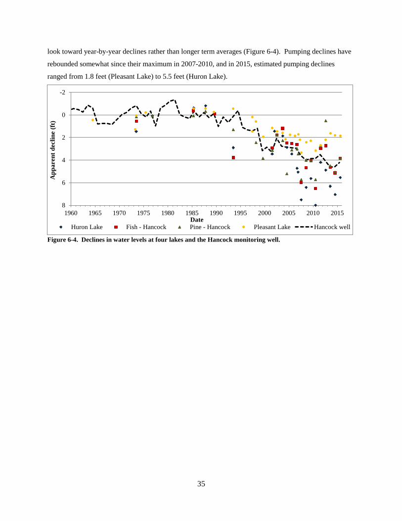
35

look toward year-by-year declines rather than longer term averages (Figure 6-4). Pumping declines have

rebounded somewhat since their maximum in 2007-2010, and in 2015, estimated pumping declines

ranged from 1.8 feet (Pleasant Lake) to 5.5 feet (Huron Lake).

Figure 6-4. Declines in water levels at four lakes and the Hancock monitoring well.

-2

0

2

4

6

81960 1965 1970 1975 1980 1985 1990 1995 2000 2005 2010 2015

App

aren

t dec

line

(ft)

DateHuron Lake Fish - Hancock Pine - Hancock Pleasant Lake Hancock well

37

7. LITTLE PLOVER RIVER 2013-2015 UPDATE

Summary

Little Plover River discharges were mostly between the public rights and historic average in

2014-2015. The public rights flow failure rate was estimated at 37% in 2014 and 53% in 2015

(Eisenhower Road continuous gauge), despite the years being quite wet.

Municipal, industrial, and the 68 irrigation wells located within two miles of the Little Plover

pumped 3.3 and 2.9 billion gallons in 2013 and 2014. Pumping for years 2013 and 2014, respectively,

was irrigation, 1.93 and 1.52 billion gallons; the Village of Plover, 521 and 540 million; Del Monte, 190

and 180 million; and the Whiting wellfield, 693 and 693 million. Plover pumping from Well 3, its well

with the least impact on the Little Plover, amounted to 59% and 71% of total Village pumping in 2013

and 2014, smaller than the goal of 80% articulated by Plover to help Little Plover discharges. Whiting

wellfield pumping remained smaller than historic amounts due to the closure of the New Page paper mill.

Little Plover diversions from municipal and industrial pumping were 1.27 cfs in 2013 and 1.15

cfs in 2014 at Hoover Road. Total diversions, including irrigation pumping (Hoover Road gauge), were

previously estimated to average 4.5 cfs.

Introduction

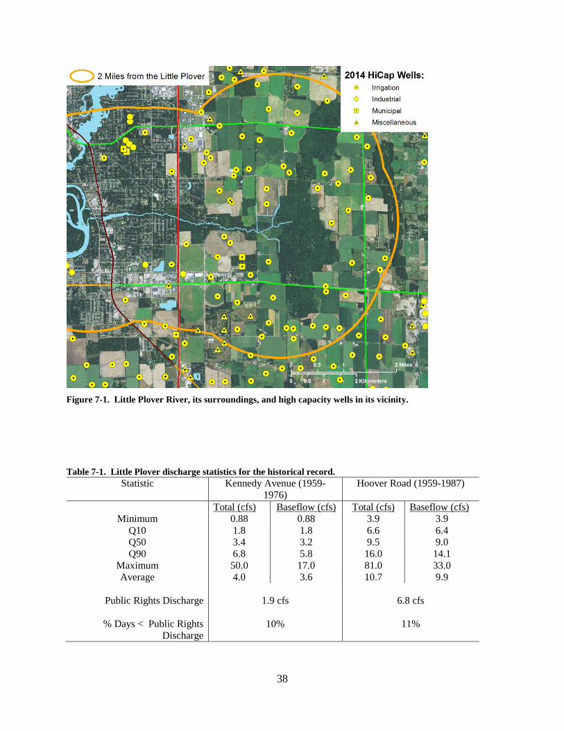
The Little Plover River (Figure 7-1) is among the more prominent of pumping-affected central

sands streams and one of the few with a lengthy continuous discharge record. Formerly renowned as a

productive trout stream (Hunt 1988) that flowed robustly even during the severest droughts (Clancy et al.

2009), the Little Plover dried in stretches during 2005-2009 when precipitation was about average to only

modestly low, and flowed below the public rights levels about half the time since 2005. Here we briefly

update the more detailed work of Clancy et al. (2009) and Kraft et al. (2012a, 2012b, 2014).

Historic discharges

The historic record of Little Plover discharges includes both USGS daily monitoring and

numerous “spot” measurements, as described in Clancy et al. (2009). The historic USGS daily record is

particularly useful and affords a basis for comparison to current conditions (Table 7-1). It comprises

measurements taken 1959-1987 at the “Little Plover at Plover” gauge (USGS # 05400650, also known as

“Hoover Road,” and 1959-1976 at the “Little Plover near Arnott” gauge (USGS #05400600, also known

as “Kennedy Avenue.” Total discharges at Hoover and Kennedy averaged 10.7 and 4.0 cfs, respectively,

baseflow discharges averaged 9.9 and 3.6 cfs, and one-day minima were 3.9 and 0.88 cfs. Minima were

measured at a time when the Little Plover was apparently already pumping affected (Clancy 2009).

38

Figure 7-1. Little Plover River, its surroundings, and high capacity wells in its vicinity. Table 7-1. Little Plover discharge statistics for the historical record.

Statistic Kennedy Avenue (1959-1976)

Hoover Road (1959-1987)

Total (cfs) Baseflow (cfs) Total (cfs) Baseflow (cfs) Minimum 0.88 0.88 3.9 3.9

Q10 1.8 1.8 6.6 6.4 Q50 3.4 3.2 9.5 9.0 Q90 6.8 5.8 16.0 14.1

Maximum 50.0 17.0 81.0 33.0 Average 4.0 3.6 10.7 9.9

Public Rights Discharge 1.9 cfs 6.8 cfs

% Days < Public Rights

Discharge

10%

11%

39

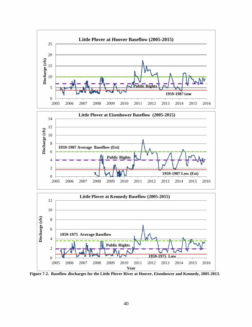
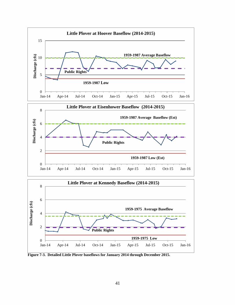
Post 2005 Discharges

Post-2005 discharges have been measured by UWSP staff during baseflow periods at roughly

monthly intervals at Hoover Road, Eisenhower Road, Kennedy Avenue (Figure 7-2 and Figure 7-3) and

occasionally other sites. A USGS gauge (# 05400625) at Eisenhower Road has also been gathering

continuous flow data since October 2013.

The baseflow record shows that 2005 to mid-2010 was a period of extremely-low flow in the

Little Plover, with discharges commonly smaller than the historic one-day low as well as the public rights

flow. Precipitation amounts then were modestly low to about average (Figure 2-1) and alone cannot

explain the small discharges. An unusual wet period spanning 2010-2011 (2010 was the third wettest

year on record, 10 inches above average) brought Little Plover flows out of extreme lows and into a

regime more representative of historic conditions. Little Plover flows once again crashed during the

summer 2012 drought, coinciding with an extreme amount of pumping. Discharges improved during

2013-2015, likely due to the wet conditions. Flows in 2014-2015 have ranged from slightly above former

one-day low flow to about average.

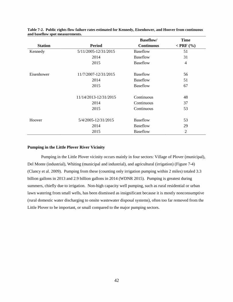
Public Rights Flow Failure Rate

Public rights flow failure rates (fraction of time that discharges were smaller than the established

public rights flow) were estimated from USGS continuous gaging data at Eisenhower Road and from

monthly baseflow measurements at Kennedy, Eisenhower, and Hoover. Failure rate estimation from

continuous data is straightforward and involves a simple tally of daily discharges less than the public

rights flow. Estimates derived from baseflows are somewhat more complicated as the data are spotty and

periods when runoff contributes to discharges is not represented. Spotty data issues were reconciled using

a linear interpolation to assign baseflow discharges to days between measurement dates. The missing of

runoff events is an inherent shortcoming in the procedure that likely biases failure rates upward.

Eisenhower public rights flow failure rates (Table 7-2) estimated from continuous data were 37%

and 53% for 2014 and 2015, respectively, while the same estimated from baseflow were 51% and 67%,

14 percentage points greater. The comparison may provide a basis for assessing bias at Eisenhower, at

least for wet years.

The 2014 failure rates estimated from baseflow data were 31% and 29% at Kennedy and Hoover,

respectively, and in 2015, 4% and 2%. Since 2005, the public rights flow failure rate based on baseflow

discharges averaged 53%.

40

Figure 7-2. Baseflow discharges for the Little Plover River at Hoover, Eisenhower and Kennedy, 2005-2013.

1959-1987 Average Baseflow

0

2

4

6

8

10

12

2005 2006 2007 2008 2009 2010 2011 2012 2013 2014 2015 2016

Dis

char

ge (c

fs)

Year

Little Plover at Kennedy Baseflow (2005-2015)

1959-1975 Average Baseflow

Public Rights

1959-1975 Low

0

2

4

6

8

10

12

14

2005 2006 2007 2008 2009 2010 2011 2012 2013 2014 2015 2016

Dis

char

ge (c

fs)

Little Plover at Eisenhower Baseflow (2005-2015)

1959-1987 Average Baseflow (Est)

Public Rights

1959-1987 Low (Est)

0

5

10

15

20

25

2005 2006 2007 2008 2009 2010 2011 2012 2013 2014 2015 2016

Dis

char

ge (c

fs)

Little Plover at Hoover Baseflow (2005-2015)

Public Rights

1959-1987 Low

41

Figure 7-3. Detailed Little Plover baseflows for January 2014 through December 2015.

0

2

4

6

8

Jan-14 Apr-14 Jul-14 Oct-14 Jan-15 Apr-15 Jul-15 Oct-15 Jan-16

Dis

char

ge (c

fs)

Little Plover at Kennedy Baseflow (2014-2015)

1959-1975 Average Baseflow

Public Rights

1959-1975 Low

0

2

4

6

8

Jan-14 Apr-14 Jul-14 Oct-14 Jan-15 Apr-15 Jul-15 Oct-15 Jan-16

Dis

char

ge (c

fs)

Little Plover at Eisenhower Baseflow (2014-2015)

1959-1987 Average Baseflow (Est)

1959-1987 Low (Est)

Public Rights

0

5

10

15

Jan-14 Apr-14 Jul-14 Oct-14 Jan-15 Apr-15 Jul-15 Oct-15 Jan-16

Dis

char

ge (c

fs)

Little Plover at Hoover Baseflow (2014-2015)

1959-1987 Average Baseflow

Public Rights

1959-1987 Low

42

Table 7-2. Public rights flow failure rates estimated for Kennedy, Eisenhower, and Hoover from continuous and baseflow spot measurements.

Station Period Baseflow/

Continuous Time

< PRF (%) Kennedy 5/11/2005-12/31/2015 Baseflow 51 2014 Baseflow 31 2015 Baseflow 4 Eisenhower 11/7/2007-12/31/2015 Baseflow 56 2014 Baseflow 51 2015 Baseflow 67 11/14/2013-12/31/2015 Continuous 48 2014 Continuous 37 2015 Continuous 53 Hoover 5/4/2005-12/31/2015 Baseflow 53 2014 Baseflow 29 2015 Baseflow 2

Pumping in the Little Plover River Vicinity

Pumping in the Little Plover vicinity occurs mainly in four sectors: Village of Plover (municipal),

Del Monte (industrial), Whiting (municipal and industrial), and agricultural (irrigation) (Figure 7-4)

(Clancy et al. 2009). Pumping from these (counting only irrigation pumping within 2 miles) totaled 3.3

billion gallons in 2013 and 2.9 billion gallons in 2014 (WDNR 2015). Pumping is greatest during

summers, chiefly due to irrigation. Non-high capacity well pumping, such as rural residential or urban

lawn watering from small wells, has been dismissed as insignificant because it is mostly nonconsumptive

(rural domestic water discharging to onsite wastewater disposal systems), often too far removed from the

Little Plover to be important, or small compared to the major pumping sectors.

43

Figure 7-4. Irrigated land, municipal and industrial high capacity wells, and Del Monte wastewater disposal areas. Plover pumping

Village of Plover pumping was 521 million gallons in 2013 and 540 million gallons in 2014

(Figure 7-5). Pumping is from three wells; Wells 1 and 2 which divert about 75% of their pumpage from

the Little Plover, and Well 3 that diverts 30% of its water from the Little Plover (Clancy et al. 2009).

Plover extracted 59% and 71% of its water from Well 3 in 2013-2014, with the remainder from Wells 1

and 2 (Figure 7-6). The Well 3 fraction is below the articulated goal of 80% to help restore some Little

Plover baseflow.

Del Monte pumping and wastewater disposal

Del Monte pumping was 190 and 180 million gallons in 2013 and 2014. Most of that pumping occurs in June through December. Three-fourths of pumped water is reportedly discharged to

44

Figure 7-5. Village of Plover total and well-by-well pumping through 2014.

Figure 7-6. Percentage of Plover pumping from Well 3. The 80% pumping level is indicated.

nearby spray fields that recharge groundwater, reducing Del Monte’s potential pumping diversions from

the Little Plover. In 2010, Del Monte moved some of its wastewater discharge closer to the Little Plover,

which further reduced its pumping impacts.

0.0

0.5

1.0

1.5

2.0

1990 1995 2000 2005 2010 2015

Mill

ion

gallo

ns p

er d

ay

Plover Well 1 Well 2 Well 3

0

20

40

60

80

100

1990 1995 2000 2005 2010 2015

Perc

ent

80%

45

Whiting wellfield

Municipal / industrial pumping from the large Whiting wellfield once supplied the Village of

Whiting and two paper mills; Neenah Papers (formerly Kimberly Clark) and New Page (formerly

Consolidated Papers), before closure of the latter. Pumpage from this wellfield was 693 million gallons

in both 2013 and 2014, a marked decline from the 1.5 billion gallons annually pumped in the previous 10

years (Figure 7-7).

Irrigation pumping

Irrigation pumping extends over a broad area with an impact that diminishes slowly with distance

from the Little Plover and in amounts that vary by crop and year. Some 68 high capacity irrigation wells

are located within two miles of the Little Plover (Figure 7-1), and these wells pumped 1.93 and 1.52

billion gallons in 2013 and 2014, respectively. Numerous high capacity irrigation wells lie beyond two

miles of the Little Plover, and these cause an estimated 18% of the Little Plover irrigation diversion

(Clancy et al. 2009).

Diversions by Municipal and Industrial Pumping

Because municipal and industrial pumping (and in the case of Del Monte, wastewater discharge)

histories are well known, their diversions from the Little Plover are directly amenable to calculation using

numerical models. These diversions were calculated using “Model 4” (Technical Memorandum #16,

Clancy et al. 2009) in transient mode with monthly stress periods beginning in 1965 and ending through

2018. For the post-2014 period, 2014 pump rates and wastewater disposal conditions were projected into

Figure 7-7. Pumping from the Whiting wellfield through December 2014.

0.0

1.0

2.0

3.0

4.0

5.0

6.0

1965 1975 1985 1995 2005 2015

Mill

ion

gallo

ns p

er d

ay

V. Whiting New Page Kimberly Clark Total

46

the future. Del Monte simulation used average pumpage and wastewater disposal (Roger Jacob email

3/3/2011); 203 million gallons distributed as 10, 48, 57, 51, 18, 12, and 7 million gallons for the months

June through December. The 79% of the Del Monte pumpage returned via spray fields as process or

cooling wastewater was modeled as an addition to the base recharge, and the monthly rate was calculated

proportional to the monthly pumpage.1

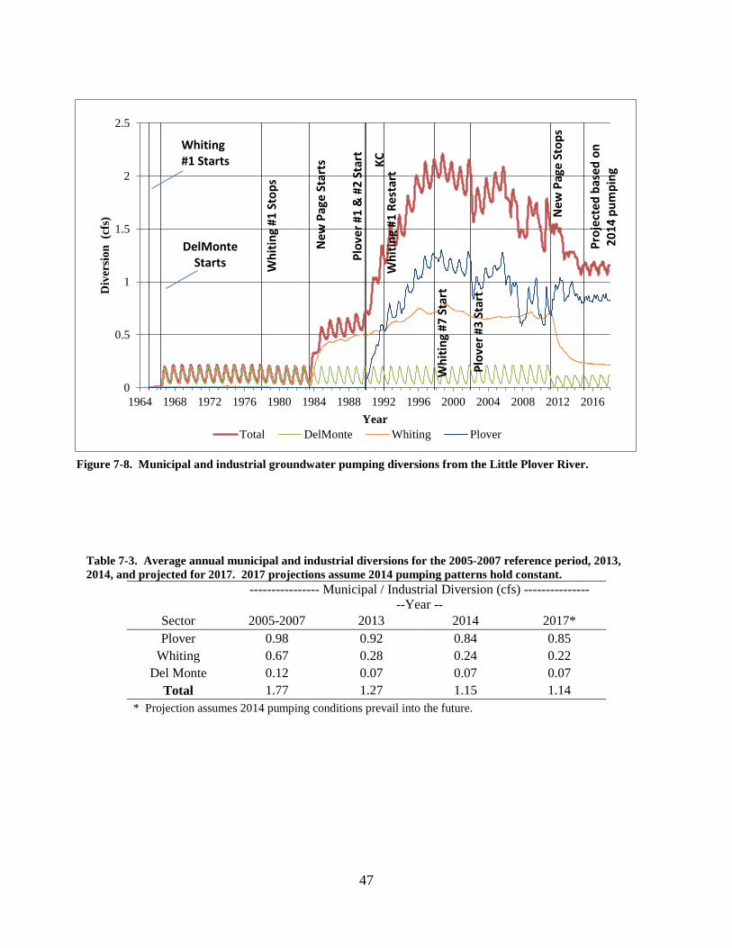
Calculated municipal and industrial diversions at Hoover Road for 1965-2014 are shown in

Figure 7-8, along with important pumping events, such as the start and stop of pumping for individual

members of the pumping sector. Total diversions were minor through 1984, about 0.12 cfs, when only

the Del Monte facility and Whiting municipal well were extracting groundwater. As groundwater

extraction increased to service other purposes (paper manufacturing by New Page / Consolidated and

Kimberly Clark / Nekoosa, Village of Plover), diversions steadily increased to about 2.2 cfs by the late

1990s. Since then, municipal and industrial diversions have experienced a decline.

Total municipal / industrial diversions were 1.27 and 1.15 cfs in 2013 and 2014, a modest

decrease from the 2005-2007 baseline of 1.77 cfs (Table 7-3). Diversions (2013/2014) by pumping entity

were Plover, 0.92/0.84 cfs; Whiting, 0.28/0.24 cfs; and Del Monte, 0.07/0.07 cfs. If 2014 pumping

patterns persist into the future (i.e., no increase in pumping rates or how pumping is apportioned among

wells), 2017 diversions (near steady-state) would be almost steady for Plover at 0.85 cfs, decrease for

Whiting to 0.22 cfs, and remain the same for Del Monte. Total diversions from the municipal and

industrial sector would be 1.14 cfs, a decline of 0.63 cfs compared to the 2005-2007 baseline, due mainly

to the New Page closure.

1 The current spray field areas (Figure 7-4) were simulated from 2010 forward. Del Monte estimated return flows of 10 million gallons cooling water to the northeast basin, 49.6 million gallons cooling water to the plant lawn fields, 37.2 million gallons wastewater to the 113 acre spray field north of the plant, 5.6 million gallons wastewater to the 17 acre spray field immediately southeast of the plant, 41.2 million gallons wastewater to the 125 acre spray field immediately south of CTH B, and 16.2 million gallons wastewater to the 49 acre spray field farthest to the south. Prior to 2011, all cooling water was returned to the plant lawn fields. The wastewater return areas have also changed over time and been modeled accordingly. Originally, all wastewater was returned to the 17 and 125 acre fields south of the plant; the 49 acre southernmost field was added later, and the northern 113 acre field was brought fully online in 2011.

47

Table 7-3. Average annual municipal and industrial diversions for the 2005-2007 reference period, 2013, 2014, and projected for 2017. 2017 projections assume 2014 pumping patterns hold constant.

---------------- Municipal / Industrial Diversion (cfs) --------------- --Year --

Sector 2005-2007 2013 2014 2017* Plover 0.98 0.92 0.84 0.85

Whiting 0.67 0.28 0.24 0.22 Del Monte 0.12 0.07 0.07 0.07

Total 1.77 1.27 1.15 1.14 * Projection assumes 2014 pumping conditions prevail into the future.

Figure 7-8. Municipal and industrial groundwater pumping diversions from the Little Plover River.

0

0.5

1

1.5

2

2.5

1964 1968 1972 1976 1980 1984 1988 1992 1996 2000 2004 2008 2012 2016

Div

ersi

on (

cfs)

YearTotal DelMonte Whiting Plover

Whiting #1 Starts

DelMonte Starts W

hitin

g #1

Sto

ps

New

Pag

e St

arts

Plov

er #

1 &

#2

Star

t

KCW

hitin

g #1

Res

tart

Whi

ting

#7 S

tart

Plov

er #

3 St

art

New

Pag

eSt

ops

Proj

ecte

d ba

sed

on20

14 p

umpi

ng

49

8. IRRIGATION RATES FOR THE CENTRAL SANDS, 2013-2014

Summary

Irrigation rates were estimated for 2013 and 2014 by sampling the pumpage, crop type, and crop

area associated with 52 irrigation wells in Portage, Waushara, and Adams Counties. Median rates among

all irrigated acreages were 9.3 inches in 2013 and 7.8 inches in 2014. Irrigation rates were greatest for

potato followed by field corn, sweet corn, and snap bean. For the 2008 through 2014 period, the annual

irrigation rate across all crops was 8.7 inches, with a range of 4.0-14.9 inches. Annual irrigation rates

correspond to the dryness of summers.

Introduction

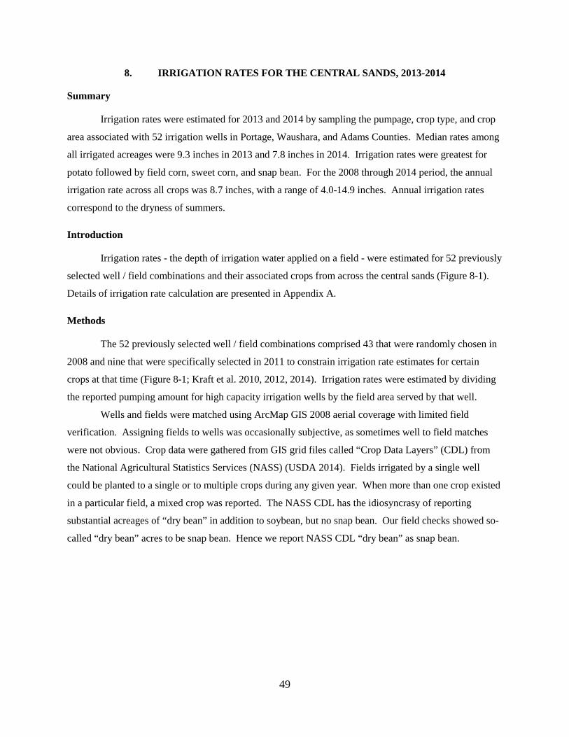
Irrigation rates - the depth of irrigation water applied on a field - were estimated for 52 previously

selected well / field combinations and their associated crops from across the central sands (Figure 8-1).

Details of irrigation rate calculation are presented in Appendix A.

Methods

The 52 previously selected well / field combinations comprised 43 that were randomly chosen in

2008 and nine that were specifically selected in 2011 to constrain irrigation rate estimates for certain

crops at that time (Figure 8-1; Kraft et al. 2010, 2012, 2014). Irrigation rates were estimated by dividing

the reported pumping amount for high capacity irrigation wells by the field area served by that well.

Wells and fields were matched using ArcMap GIS 2008 aerial coverage with limited field

verification. Assigning fields to wells was occasionally subjective, as sometimes well to field matches

were not obvious. Crop data were gathered from GIS grid files called “Crop Data Layers” (CDL) from

the National Agricultural Statistics Services (NASS) (USDA 2014). Fields irrigated by a single well

could be planted to a single or to multiple crops during any given year. When more than one crop existed

in a particular field, a mixed crop was reported. The NASS CDL has the idiosyncrasy of reporting

substantial acreages of “dry bean” in addition to soybean, but no snap bean. Our field checks showed so-

called “dry bean” acres to be snap bean. Hence we report NASS CDL “dry bean” as snap bean.

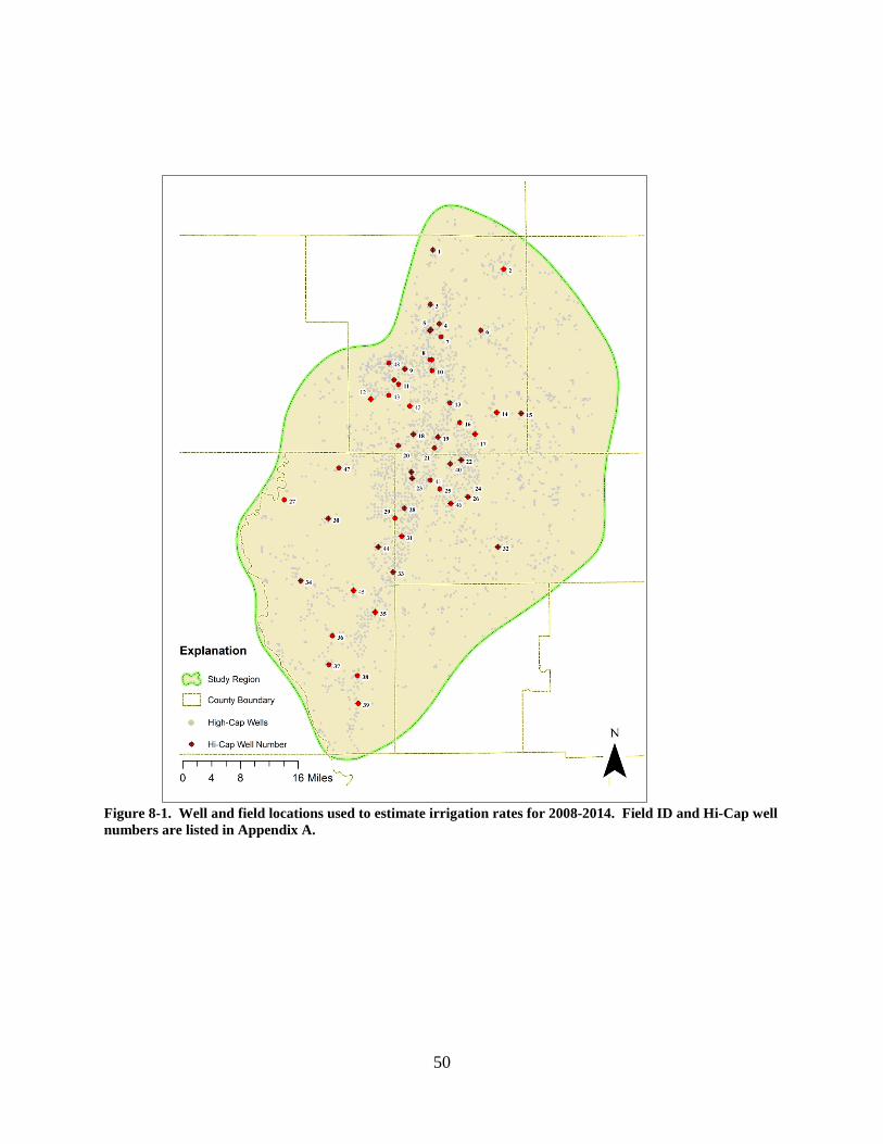
50

Figure 8-1. Well and field locations used to estimate irrigation rates for 2008-2014. Field ID and Hi-Cap well numbers are listed in Appendix A.

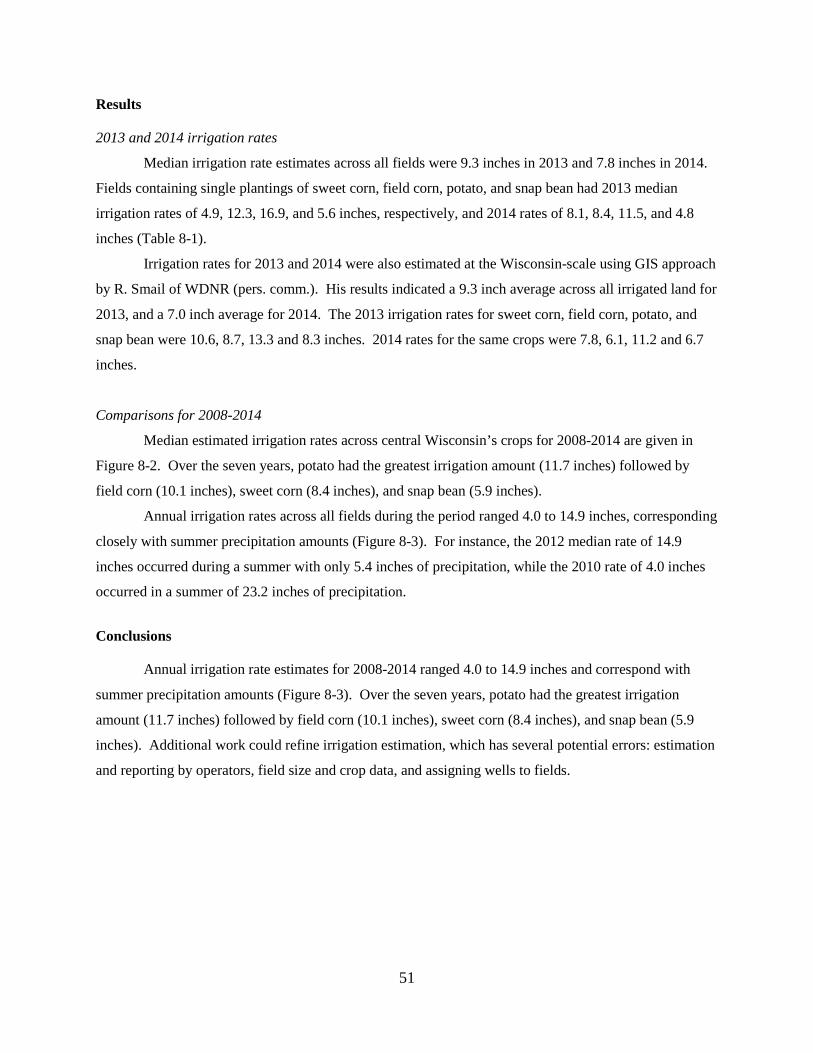
51

Results

2013 and 2014 irrigation rates

Median irrigation rate estimates across all fields were 9.3 inches in 2013 and 7.8 inches in 2014.

Fields containing single plantings of sweet corn, field corn, potato, and snap bean had 2013 median

irrigation rates of 4.9, 12.3, 16.9, and 5.6 inches, respectively, and 2014 rates of 8.1, 8.4, 11.5, and 4.8

inches (Table 8-1).

Irrigation rates for 2013 and 2014 were also estimated at the Wisconsin-scale using GIS approach

by R. Smail of WDNR (pers. comm.). His results indicated a 9.3 inch average across all irrigated land for

2013, and a 7.0 inch average for 2014. The 2013 irrigation rates for sweet corn, field corn, potato, and

snap bean were 10.6, 8.7, 13.3 and 8.3 inches. 2014 rates for the same crops were 7.8, 6.1, 11.2 and 6.7

inches.

Comparisons for 2008-2014

Median estimated irrigation rates across central Wisconsin’s crops for 2008-2014 are given in

Figure 8-2. Over the seven years, potato had the greatest irrigation amount (11.7 inches) followed by

field corn (10.1 inches), sweet corn (8.4 inches), and snap bean (5.9 inches).

Annual irrigation rates across all fields during the period ranged 4.0 to 14.9 inches, corresponding

closely with summer precipitation amounts (Figure 8-3). For instance, the 2012 median rate of 14.9

inches occurred during a summer with only 5.4 inches of precipitation, while the 2010 rate of 4.0 inches

occurred in a summer of 23.2 inches of precipitation.

Conclusions

Annual irrigation rate estimates for 2008-2014 ranged 4.0 to 14.9 inches and correspond with

summer precipitation amounts (Figure 8-3). Over the seven years, potato had the greatest irrigation

amount (11.7 inches) followed by field corn (10.1 inches), sweet corn (8.4 inches), and snap bean (5.9

inches). Additional work could refine irrigation estimation, which has several potential errors: estimation

and reporting by operators, field size and crop data, and assigning wells to fields.

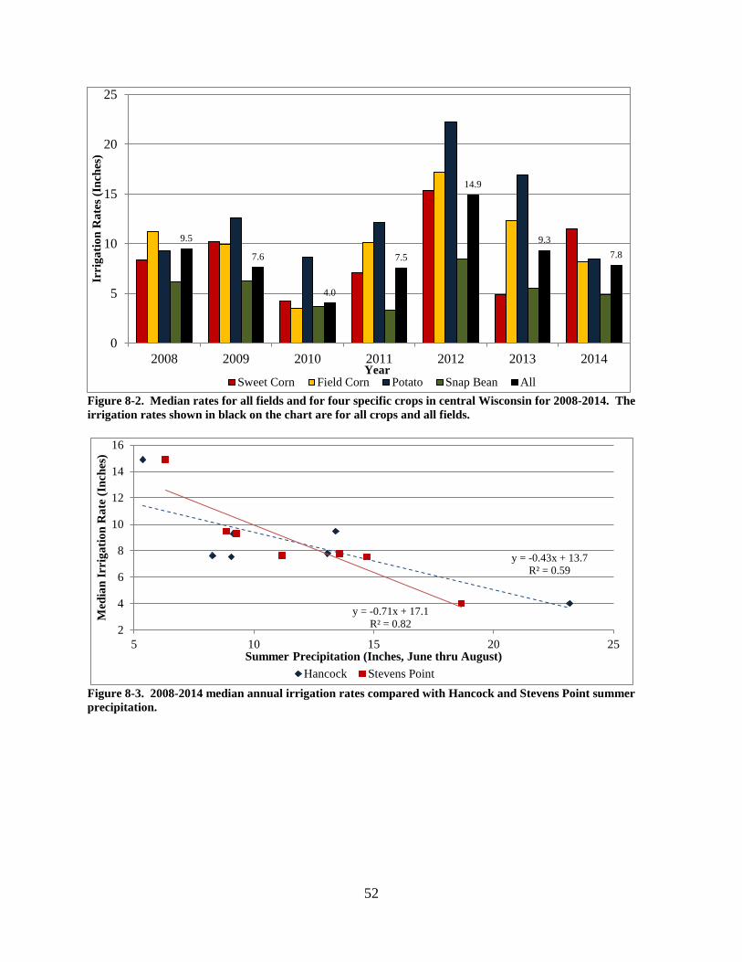
52

Figure 8-2. Median rates for all fields and for four specific crops in central Wisconsin for 2008-2014. The irrigation rates shown in black on the chart are for all crops and all fields.

Figure 8-3. 2008-2014 median annual irrigation rates compared with Hancock and Stevens Point summer precipitation.

9.5

7.6

4.0

7.5

14.9

9.37.8

0

5

10

15

20

25

2008 2009 2010 2011 2012 2013 2014

Irri

gatio

n R

ates

(Inc

hes)

YearSweet Corn Field Corn Potato Snap Bean All

y = -0.43x + 13.7R² = 0.59

y = -0.71x + 17.1R² = 0.822

4

6

8

10

12

14

16

5 10 15 20 25

Med

ian

Irri

gatio

n R

ate

(Inc

hes)

Summer Precipitation (Inches, June thru August)Hancock Stevens Point

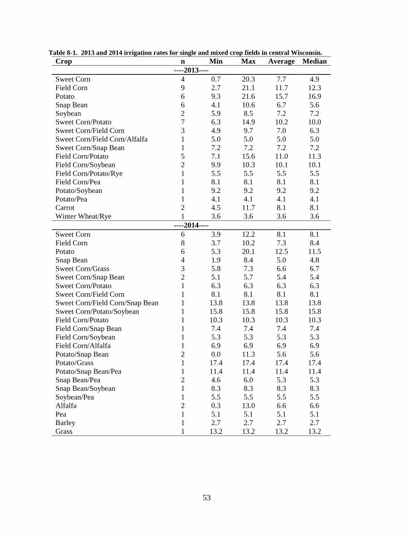
53

Table 8-1. 2013 and 2014 irrigation rates for single and mixed crop fields in central Wisconsin. Crop n Min Max Average Median

----2013---- Sweet Corn 4 0.7 20.3 7.7 4.9 Field Corn 9 2.7 21.1 11.7 12.3 Potato 6 9.3 21.6 15.7 16.9 Snap Bean 6 4.1 10.6 6.7 5.6 Soybean 2 5.9 8.5 7.2 7.2 Sweet Corn/Potato 7 6.3 14.9 10.2 10.0 Sweet Corn/Field Corn 3 4.9 9.7 7.0 6.3 Sweet Corn/Field Corn/Alfalfa 1 5.0 5.0 5.0 5.0 Sweet Corn/Snap Bean 1 7.2 7.2 7.2 7.2 Field Corn/Potato 5 7.1 15.6 11.0 11.3 Field Corn/Soybean 2 9.9 10.3 10.1 10.1 Field Corn/Potato/Rye 1 5.5 5.5 5.5 5.5 Field Corn/Pea 1 8.1 8.1 8.1 8.1 Potato/Soybean 1 9.2 9.2 9.2 9.2 Potato/Pea 1 4.1 4.1 4.1 4.1 Carrot 2 4.5 11.7 8.1 8.1 Winter Wheat/Rye 1 3.6 3.6 3.6 3.6

----2014---- Sweet Corn 6 3.9 12.2 8.1 8.1 Field Corn 8 3.7 10.2 7.3 8.4 Potato 6 5.3 20.1 12.5 11.5 Snap Bean 4 1.9 8.4 5.0 4.8 Sweet Corn/Grass 3 5.8 7.3 6.6 6.7 Sweet Corn/Snap Bean 2 5.1 5.7 5.4 5.4 Sweet Corn/Potato 1 6.3 6.3 6.3 6.3 Sweet Corn/Field Corn 1 8.1 8.1 8.1 8.1 Sweet Corn/Field Corn/Snap Bean 1 13.8 13.8 13.8 13.8 Sweet Corn/Potato/Soybean 1 15.8 15.8 15.8 15.8 Field Corn/Potato 1 10.3 10.3 10.3 10.3 Field Corn/Snap Bean 1 7.4 7.4 7.4 7.4 Field Corn/Soybean 1 5.3 5.3 5.3 5.3 Field Corn/Alfalfa 1 6.9 6.9 6.9 6.9 Potato/Snap Bean 2 0.0 11.3 5.6 5.6 Potato/Grass 1 17.4 17.4 17.4 17.4 Potato/Snap Bean/Pea 1 11.4 11.4 11.4 11.4 Snap Bean/Pea 2 4.6 6.0 5.3 5.3 Snap Bean/Soybean 1 8.3 8.3 8.3 8.3 Soybean/Pea 1 5.5 5.5 5.5 5.5 Alfalfa 2 0.3 13.0 6.6 6.6 Pea 1 5.1 5.1 5.1 5.1 Barley 1 2.7 2.7 2.7 2.7 Grass 1 13.2 13.2 13.2 13.2

54

LITERATURE CITED Clancy, K., G.J. Kraft, and D.J. Mechenich. 2009. Knowledge Development for Groundwater Withdrawal Management around the Little Plover River, Portage County Wisconsin. Center for Watershed Science and Education, University of Wisconsin, Stevens Point, WI. Haucke, J. 2010. Precipitation and Pumping Effects on Groundwater Levels in Central Wisconsin. Masters of Science Thesis, University of Wisconsin – Stevens Point. Stevens Point, WI. Hunt, R.L. 1988. A Compendium of 45 Trout Stream Habitat Development Evaluations in Wisconsin During 1953-1985. Wisconsin Department of Natural Resources Technical Bulletin 162:1-80. Juckem, P.F., R.J. Hunt, M.P. Anderson, and D.M. Robertson. 2008. Effects of Climate and Land Management Change on Streamflow in the Driftless Area of Wisconsin. Journal of Hydrology 355:123–130. doi:10.1016/j.jhydrol.2008.03.010. Kraft, G.J., D.J. Mechenich, K. Clancy, and J. Haucke. 2010. Groundwater Pumping Effects on Groundwater Levels, Lake Levels, and Streamflows in the Wisconsin Central Sands. Center for Watershed Science and Education, University of Wisconsin, Stevens Point, WI. Kraft, G.J., D.J. Mechenich, and J. Haucke. 2012a. Information Support for Groundwater Management in the Wisconsin Central Sands, 2009 – 2011. Center for Watershed Science and Education, University of Wisconsin, Stevens Point, WI. Kraft, G.J., D.J. Mechenich, and J. Haucke. 2014. Information Support for Groundwater Management in the Wisconsin Central Sands, 2011 – 2013. Center for Watershed Science and Education, University of Wisconsin, Stevens Point, WI. Kraft, G.J., K. Clancy, and D.J. Mechenich. 2008. A Survey of Baseflow Discharges in the Western Fox-Wolf Watershed. Center for Watershed Science and Education, University of Wisconsin, Stevens Point, WI. Kraft, G.J., K. Clancy, D.J. Mechenich, and J. Haucke. 2012b. Irrigation Effects in the Northern Lake States: Wisconsin Central Sands Revisited. Ground Water Journal 50 (2):308-318. Serbin, S.P. and C.J. Kucharik. 2009. Spatio-temporal mapping of daily temperature and precipitation for the development of a multi-decadal climatic dataset for Wisconsin. Journal of Applied Meteorology and Climatology 48 (4):742-757. USDA. NASS (National Agricultural Statistical Service). 2014. CropScape – Cropland Data Layer. http://nassgeodata.gmu.edu/CropScape/. WDNR (Wisconsin Department of Natural Resources). 2009. In the Matter of the Establishment of Public Rights Stage(s) / Flow(s) for the Little Plover River, Portage County. http://dnr.wi.gov/water/basin/cwrb/little%20plover%20river %20public% 20rights %20flow%20order.pdf WDNR (Wisconsin Department of Natural Resources). 2015. Water Use Reporting. Water Use Section, Madison, WI. WICCI (Wisconsin Initiative on Climate Change Impacts). 2011. Wisconsin’s Changing Climate: Impacts and Adaptations. Nelson Institute for Environmental Studies, University of Wisconsin-Madison and the Wisconsin Department of Natural Resources, Madison, WI. Wisconsin State Climatology Office. 2016. Central Wisconsin Palmer drought severity index. www.aos.wisc.edu/~sco.

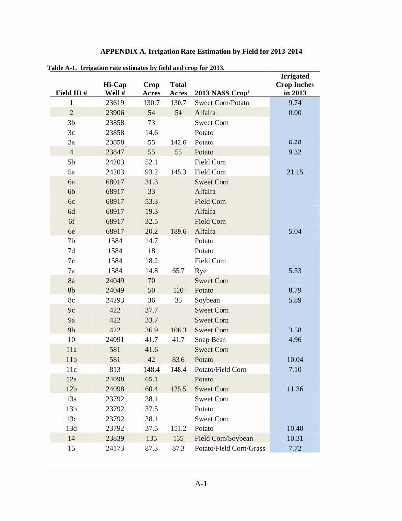
A-1

APPENDIX A. Irrigation Rate Estimation by Field for 2013-2014

Table A-1. Irrigation rate estimates by field and crop for 2013.

Field ID # Hi-Cap Well #

Crop Acres

Total Acres 2013 NASS Crop1

Irrigated Crop Inches

in 2013 1 23619 130.7 130.7 Sweet Corn/Potato 9.74 2 23906 54 54 Alfalfa 0.00

3b 23858 73 Sweet Corn 3c 23858 14.6 Potato 3a 23858 55 142.6 Potato 6.28 4 23847 55 55 Potato 9.32

5b 24203 52.1 Field Corn 5a 24203 93.2 145.3 Field Corn 21.15 6a 68917 31.3 Sweet Corn 6b 68917 33 Alfalfa 6c 68917 53.3 Field Corn 6d 68917 19.3 Alfalfa 6f 68917 32.5 Field Corn 6e 68917 20.2 189.6 Alfalfa 5.04 7b 1584 14.7 Potato 7d 1584 18 Potato 7c 1584 18.2 Field Corn 7a 1584 14.8 65.7 Rye 5.53 8a 24049 70 Sweet Corn 8b 24049 50 120 Potato 8.79 8c 24293 36 36 Soybean 5.89 9c 422 37.7 Sweet Corn 9a 422 33.7 Sweet Corn 9b 422 36.9 108.3 Sweet Corn 3.58 10 24091 41.7 41.7 Snap Bean 4.96 11a 581 41.6 Sweet Corn 11b 581 42 83.6 Potato 10.04 11c 813 148.4 148.4 Potato/Field Corn 7.10 12a 24098 65.1 Potato 12b 24098 60.4 125.5 Sweet Corn 11.36 13a 23792 38.1 Sweet Corn 13b 23792 37.5 Potato 13c 23792 38.1 Sweet Corn 13d 23792 37.5 151.2 Potato 10.40 14 23839 135 135 Field Corn/Soybean 10.31 15 24173 87.3 87.3 Potato/Field Corn/Grass 7.72

A-2

Table A-1. Irrigation rate estimates by field and crop for 2013, continued

Field ID # Hi-Cap Well #

Crop Acres

Total Acres 2013 NASS Crop1

Irrigated Crop Inches

in 2013 16a 23602 62.3 Pea 16b 23602 63.1 125.4 Field Corn 8.13 17a 24014 34.8 Sweet Corn 17b 24014 56.2 Sweet Corn 17c 24014 64 155 Snap Bean 7.23 18 23666 148 148 Carrot 11.70 19 23711/23607 36 Field Corn 19 23711/23607 119 155 Field Corn 2.70

20b 411 30.9 Potato 20a 411 51 Potato 20c 411 50.7 132.6 Soybean 9.16 21a 911 32.8 Field Corn 21b 911 35.2 Field Corn 21c 911 72.3 140.3 Field Corn 11.15 22 36394 146.4 146.4 Snap Bean 4.10

23b 36666 30.6 Potato 23a 36666 29.1 Potato 23c 36666 33.8 93.5 Sweet Corn 14.93 23d 1650 144.8 144.8 Sweet Corn 6.14 24 36550 154.2 154.2 Potato 14.95 25a 36728 28.6 Potato 25b 36728 37 Potato 25c 36728 39.7 Potato 25e 36728 34 Potato 25f 36728 75.7 Potato 25d 36728 37.3 252.3 Field Corn 11.35 26b 67319 69.4 Potato 26a 67319 68.9 138.3 Potato 10.43 27 64 124.2 124.2 Snap Bean 9.74

28b 36454 75.8 Field Corn 28a 36454 110.3 186.1 Field Corn 8.86 29b 36720 113 Field Corn 29a 36720 150 263 Potato 13.19 30b 258 37.4 Potato 30c 258 35.4 Potato 30a 258 72.9 145.7 Field Corn 15.61 31b 36508 74.2 Soybean 31a 36508 114 188.2 Soybean 8.48 32 36529 149.2 149.2 Field Corn/Soybean 9.87

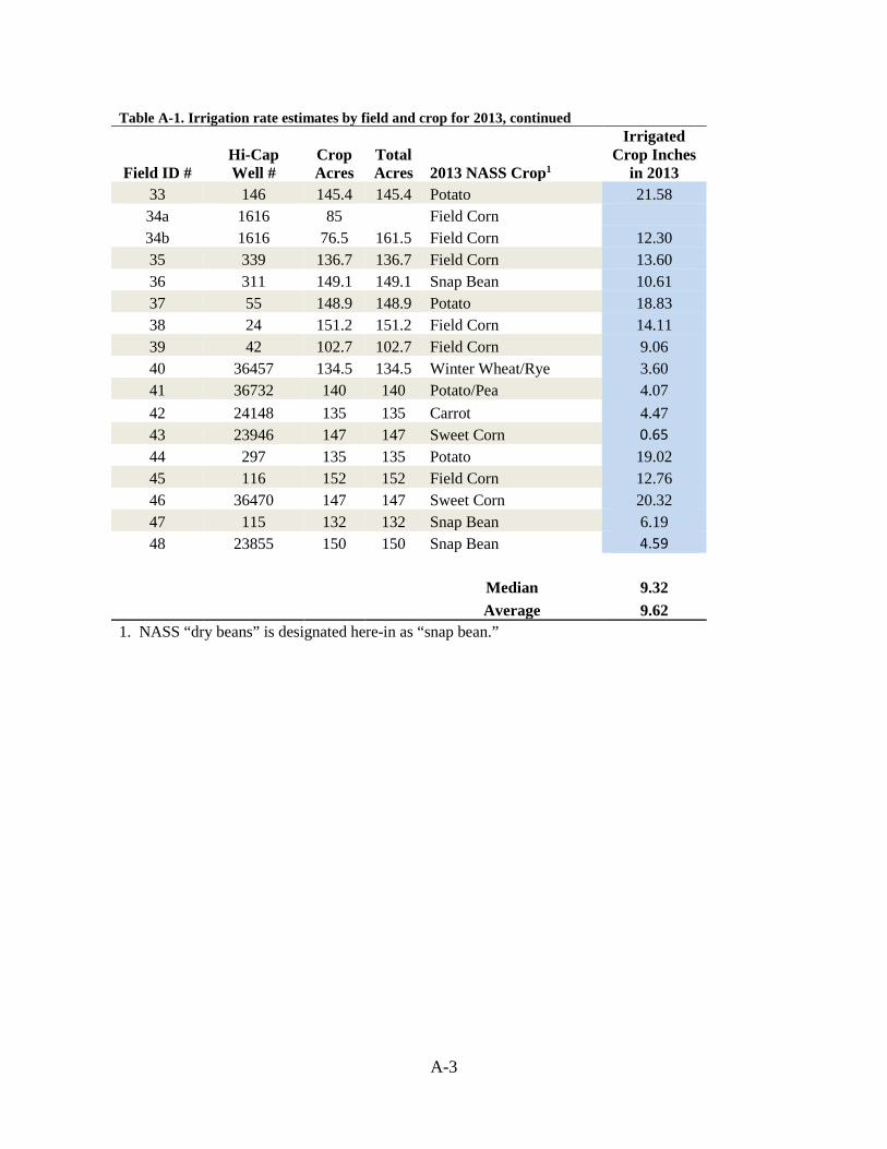
A-3

Table A-1. Irrigation rate estimates by field and crop for 2013, continued

Field ID # Hi-Cap Well #

Crop Acres

Total Acres 2013 NASS Crop1

Irrigated Crop Inches

in 2013 33 146 145.4 145.4 Potato 21.58 34a 1616 85 Field Corn 34b 1616 76.5 161.5 Field Corn 12.30 35 339 136.7 136.7 Field Corn 13.60 36 311 149.1 149.1 Snap Bean 10.61 37 55 148.9 148.9 Potato 18.83 38 24 151.2 151.2 Field Corn 14.11 39 42 102.7 102.7 Field Corn 9.06 40 36457 134.5 134.5 Winter Wheat/Rye 3.60 41 36732 140 140 Potato/Pea 4.07 42 24148 135 135 Carrot 4.47 43 23946 147 147 Sweet Corn 0.65 44 297 135 135 Potato 19.02 45 116 152 152 Field Corn 12.76 46 36470 147 147 Sweet Corn 20.32 47 115 132 132 Snap Bean 6.19 48 23855 150 150 Snap Bean 4.59

Median 9.32 Average 9.62

1. NASS “dry beans” is designated here-in as “snap bean.”

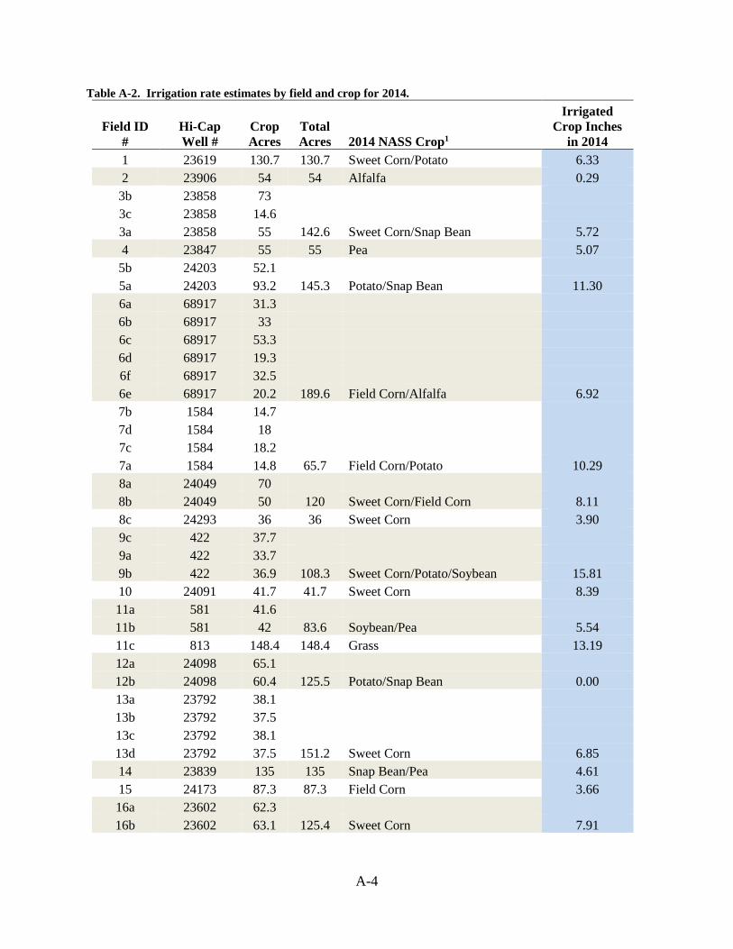
A-4

Table A-2. Irrigation rate estimates by field and crop for 2014.

Field ID #

Hi-Cap Well #

Crop Acres

Total Acres 2014 NASS Crop1

Irrigated Crop Inches

in 2014 1 23619 130.7 130.7 Sweet Corn/Potato 6.33 2 23906 54 54 Alfalfa 0.29

3b 23858 73 3c 23858 14.6 3a 23858 55 142.6 Sweet Corn/Snap Bean 5.72 4 23847 55 55 Pea 5.07

5b 24203 52.1 5a 24203 93.2 145.3 Potato/Snap Bean 11.30 6a 68917 31.3 6b 68917 33 6c 68917 53.3 6d 68917 19.3 6f 68917 32.5 6e 68917 20.2 189.6 Field Corn/Alfalfa 6.92 7b 1584 14.7 7d 1584 18 7c 1584 18.2 7a 1584 14.8 65.7 Field Corn/Potato 10.29 8a 24049 70 8b 24049 50 120 Sweet Corn/Field Corn 8.11 8c 24293 36 36 Sweet Corn 3.90 9c 422 37.7 9a 422 33.7 9b 422 36.9 108.3 Sweet Corn/Potato/Soybean 15.81 10 24091 41.7 41.7 Sweet Corn 8.39 11a 581 41.6 11b 581 42 83.6 Soybean/Pea 5.54 11c 813 148.4 148.4 Grass 13.19 12a 24098 65.1 12b 24098 60.4 125.5 Potato/Snap Bean 0.00 13a 23792 38.1 13b 23792 37.5 13c 23792 38.1 13d 23792 37.5 151.2 Sweet Corn 6.85 14 23839 135 135 Snap Bean/Pea 4.61 15 24173 87.3 87.3 Field Corn 3.66 16a 23602 62.3 16b 23602 63.1 125.4 Sweet Corn 7.91

A-5

Table A-2. Irrigation rate estimates by field and crop for 2014, continued.

Field ID #

Hi-Cap Well #

Crop Acres

Total Acres 2014 NASS Crop1

Irrigated Crop Inches

in 2014 17a 24014 34.8 17b 24014 56.2 17c 24014 64 155 Field Corn 4.67 18 23666 148 148 Sweet Corn/Snap Bean 5.09 19 23711/23607 36 19 23711/23607 119 155 Snap Bean 3.00 20b 411 30.9 20a 411 51 20c 411 50.7 132.6 Sweet Corn/Field Corn/Snap Bean 13.83 21a 911 32.8 21b 911 35.2 21c 911 72.3 140.3 Snap Bean/Soybean 8.25 22 36394 146.4 146.4 Sweet Corn 9.27 23b 36666 30.6 23a 36666 29.1 23c 36666 33.8 93.5 Snap Bean 6.66 23d 1650 144.8 144.8 Potato 5.27 24 36550 154.2 154.2 Sweet Corn/Grass 6.73 25a 36728 28.6 25b 36728 37 25c 36728 39.7 25e 36728 34 25f 36728 75.7 25d 36728 37.3 252.3 Field Corn 7.82 26b 67319 69.4 26a 67319 68.9 138.3 Barley 2.71 27 64 124.2 124.2 Potato 20.11 28b 36454 75.8 28a 36454 110.3 186.1 Field Corn 9.81 29b 36720 113 29a 36720 150 263 Field Corn 4.07 30b 258 37.4 30c 258 35.4 30a 258 72.9 145.7 Potato/Grass 17.37 31b 36508 74.2 31a 36508 114 188.2 Snap Bean/Pea 6.00 32 36529 149.2 149.2 Potato 12.68 33 146 145.4 145.4 Field Corn 9.13 34a 1616 85

A-6

Table A-2. Irrigation rate estimates by field and crop for 2014, continued.

Field ID #

Hi-Cap Well #

Crop Acres

Total Acres 2014 NASS Crop1

Irrigated Crop Inches

in 2014 34b 1616 76.5 161.5 Field Corn/Snap Bean 7.38 35 339 136.7 136.7 Snap Bean 8.42 36 311 149.1 149.1 Alfalfa 13.00 37 55 148.9 148.9 Field Corn 10.21 38 24 151.2 151.2 Potato 16.76 39 42 102.7 102.7 Field Corn/Soybean 5.28 40 36457 134.5 134.5 Snap Bean 1.87 41 36732 140 140 Potato/Snap Bean/Pea 11.37 42 24148 135 135 Potato 10.07 43 23946 147 147 Potato 10.31 44 297 135 135 Sweet Corn/Grass 5.84 45 116 152 152 Field Corn 9.06 46 36470 147 147 Potato/Dry Bean/Soybean/Grass 14.57 47 115 132 132 Sweet Corn 12.24 48 23855 150 150 Sweet Corn/Grass 7.30

Median 7.82 Average 8.24

1. NASS “dry beans” is designated here-in as “snap bean.”