INFORMATION ON ONLINE SOCIAL NETWORKS

INFORMATION ONONLINE SOCIAL NETWORKS

A THESIS SUBMITTED TO THE UNIVERSITY OF MANCHESTER

FOR THE DEGREE OF DOCTOR OF PHILOSOPHY

IN THE FACULTY OF HUMANITIES

2021

Lois M. SimanjuntakSchool of Social Sciences

Economics

Contents

Abstract 8

Declaration 9

Copyright 10

Dedication 11

Acknowledgements 12

Publications from this thesis 13

1 Introduction 141.1 Background and motivation . . . . . . . . . . . . . . . . . . . . . . . . . . . . . . 14

1.2 Organisation of thesis . . . . . . . . . . . . . . . . . . . . . . . . . . . . . . . . . 17

2 Social information and consumer heterogeneity 192.1 Introduction . . . . . . . . . . . . . . . . . . . . . . . . . . . . . . . . . . . . . . 19

2.2 Related literature . . . . . . . . . . . . . . . . . . . . . . . . . . . . . . . . . . . 21

2.3 Setup . . . . . . . . . . . . . . . . . . . . . . . . . . . . . . . . . . . . . . . . . 23

2.4 Results . . . . . . . . . . . . . . . . . . . . . . . . . . . . . . . . . . . . . . . . . 25

2.5 Concluding remarks . . . . . . . . . . . . . . . . . . . . . . . . . . . . . . . . . . 32

3 Social information and consumer heterogeneity: extensions 343.1 Extension to groups of consumers . . . . . . . . . . . . . . . . . . . . . . . . . . 35

3.2 Extension to level of responsiveness to advertising . . . . . . . . . . . . . . . . . . 42

3.3 Extension to number of expenditures . . . . . . . . . . . . . . . . . . . . . . . . . 46

3.4 Extension to sampling procedure . . . . . . . . . . . . . . . . . . . . . . . . . . . 49

3.4.1 Search with possibility of betting . . . . . . . . . . . . . . . . . . . . . . 49

3.4.2 Consumers’ search rule . . . . . . . . . . . . . . . . . . . . . . . . . . . . 50

2

3.4.3 Equilibrium advertising expenditures . . . . . . . . . . . . . . . . . . . . 55

4 Rational spoiling through reviews 654.1 Introduction . . . . . . . . . . . . . . . . . . . . . . . . . . . . . . . . . . . . . . 65

4.2 Related literature . . . . . . . . . . . . . . . . . . . . . . . . . . . . . . . . . . . 66

4.3 Model . . . . . . . . . . . . . . . . . . . . . . . . . . . . . . . . . . . . . . . . . 69

4.3.1 Information structure . . . . . . . . . . . . . . . . . . . . . . . . . . . . . 69

4.3.2 Strategies and payoffs . . . . . . . . . . . . . . . . . . . . . . . . . . . . 70

4.3.3 Timing . . . . . . . . . . . . . . . . . . . . . . . . . . . . . . . . . . . . 72

4.3.4 Equilibrium concept . . . . . . . . . . . . . . . . . . . . . . . . . . . . . 72

4.3.5 Optimal pricing policy . . . . . . . . . . . . . . . . . . . . . . . . . . . . 74

4.4 Analysis . . . . . . . . . . . . . . . . . . . . . . . . . . . . . . . . . . . . . . . . 75

4.4.1 Review with spoilers, homogeneous consumers . . . . . . . . . . . . . . . 75

4.4.2 Review with spoilers, heterogeneous consumers . . . . . . . . . . . . . . . 76

4.4.3 Benchmark case: review without spoilers . . . . . . . . . . . . . . . . . . 83

4.4.4 Consumer welfare . . . . . . . . . . . . . . . . . . . . . . . . . . . . . . 86

4.4.5 Endogenous spoiling . . . . . . . . . . . . . . . . . . . . . . . . . . . . . 90

4.5 Extensions . . . . . . . . . . . . . . . . . . . . . . . . . . . . . . . . . . . . . . . 93

4.5.1 Mixed strategy in homogeneous consumers case . . . . . . . . . . . . . . 93

4.5.2 Mandated uniform pricing . . . . . . . . . . . . . . . . . . . . . . . . . . 94

4.6 Discussion . . . . . . . . . . . . . . . . . . . . . . . . . . . . . . . . . . . . . . . 97

4.7 Conclusion . . . . . . . . . . . . . . . . . . . . . . . . . . . . . . . . . . . . . . 101

5 Concluding remarks 103

A Appendix to Chapter 2 105A.1 Proof of Proposition 1 . . . . . . . . . . . . . . . . . . . . . . . . . . . . . . . . . 105

A.2 Proof of Proposition 2 . . . . . . . . . . . . . . . . . . . . . . . . . . . . . . . . . 106




B Appendix to Chapter 3 113B.1 Proof of Proposition 6 . . . . . . . . . . . . . . . . . . . . . . . . . . . . . . . . . 113

B.2 Proof of Proposition 7 . . . . . . . . . . . . . . . . . . . . . . . . . . . . . . . . . 117



3

B.5 Proof of Proposition 10 . . . . . . . . . . . . . . . . . . . . . . . . . . . . . . . . 122B.6 Proof of Proposition 11 . . . . . . . . . . . . . . . . . . . . . . . . . . . . . . . . 126B.7 Proof of Proposition 12 . . . . . . . . . . . . . . . . . . . . . . . . . . . . . . . . 126B.8 Proof of Proposition 13 . . . . . . . . . . . . . . . . . . . . . . . . . . . . . . . . 127B.9 Proof of Proposition 14 . . . . . . . . . . . . . . . . . . . . . . . . . . . . . . . . 128B.10 Proof of Proposition 15 . . . . . . . . . . . . . . . . . . . . . . . . . . . . . . . . 128B.11 Proof of Proposition 16 . . . . . . . . . . . . . . . . . . . . . . . . . . . . . . . . 129B.12 Proof of Proposition 17 . . . . . . . . . . . . . . . . . . . . . . . . . . . . . . . . 131B.13 Proof of Proposition 18 . . . . . . . . . . . . . . . . . . . . . . . . . . . . . . . . 132B.14 Proof of Proposition 19 . . . . . . . . . . . . . . . . . . . . . . . . . . . . . . . . 134

C Appendix to Chapter 4 137C.1 Proof of Proposition 20 . . . . . . . . . . . . . . . . . . . . . . . . . . . . . . . . 137

C.1.1 Consumers’ best response function . . . . . . . . . . . . . . . . . . . . . 137C.1.2 Consumer equilibrium with homogeneous consumers . . . . . . . . . . . . 141C.1.3 Stackelberg equilibrium with homogeneous consumers . . . . . . . . . . . 142

C.2 Proof of Proposition 21 . . . . . . . . . . . . . . . . . . . . . . . . . . . . . . . . 143C.2.1 Consumers’ best response function . . . . . . . . . . . . . . . . . . . . . 143C.2.2 Consumer equilibrium with heterogeneous consumers . . . . . . . . . . . 143C.2.3 Stackelberg equilibrium with heterogeneous consumers . . . . . . . . . . . 144

C.3 Proof of Proposition 22 . . . . . . . . . . . . . . . . . . . . . . . . . . . . . . . . 146C.4 Proof of Proposition 23 . . . . . . . . . . . . . . . . . . . . . . . . . . . . . . . . 147C.5 Proof of Proposition 24 . . . . . . . . . . . . . . . . . . . . . . . . . . . . . . . . 148C.6 Proof of Proposition 25 . . . . . . . . . . . . . . . . . . . . . . . . . . . . . . . . 150C.7 Proof of Proposition 26 . . . . . . . . . . . . . . . . . . . . . . . . . . . . . . . . 153C.8 Proof of Proposition 27 . . . . . . . . . . . . . . . . . . . . . . . . . . . . . . . . 161C.9 Proof of Proposition 28 . . . . . . . . . . . . . . . . . . . . . . . . . . . . . . . . 163

Word Count: 32586

4

List of Tables

1.1 Role of consumer heterogeneity revealed in the thesis . . . . . . . . . . . . . . . . 16

4.1 Consumer i’s expected payoff ui(si,s−i,p) . . . . . . . . . . . . . . . . . . . . . . 714.2 Examples of experience goods with attributes affecting enjoyment . . . . . . . . . 101

C.1 Consumer i’s best response function given each area (set of price vectors p(α,π,vi) )140C.2 Equilibrium strategies in each area (set of price vectors p(α,π,v) ) . . . . . . . . . 141C.3 Equilibrium outcome and expected revenue for each possible intersection of sets

of price vectors . . . . . . . . . . . . . . . . . . . . . . . . . . . . . . . . . . . . 144C.4 Expected revenue of firm and expected consumer surplus for each case with same

valuation v . . . . . . . . . . . . . . . . . . . . . . . . . . . . . . . . . . . . . . . 148C.5 Expected revenue and expected consumer surplus for each candidate set . . . . . . 149C.6 Optimal level of spoiling for consumers . . . . . . . . . . . . . . . . . . . . . . . 153C.7 Consumer i’s best response function given each area (set of price vectors p(α,π,vi) )162C.8 Equilibrium strategies of consumers and equilibrium outcome in each price range . 163C.9 Equilibrium outcome and expected revenue for each possible intersection of price

ranges . . . . . . . . . . . . . . . . . . . . . . . . . . . . . . . . . . . . . . . . . 164

5

List of Figures

2.1 Illustration of areas of the three types of equilibrium (Proposition 1) . . . . . . . . 28

3.1 Illustration of equilibrium with two consumer groups . . . . . . . . . . . . . . . . 36

3.2 Illustration of model with M groups . . . . . . . . . . . . . . . . . . . . . . . . . 37

3.3 Illustration of equilibrium with three consumer groups (Proposition 6) . . . . . . . 39

3.4 Equilibrium characterisation with three consumer groups, if f0,1 = 0 . . . . . . . . 39

3.5 Equilibrium characterisation with three consumer groups, if f0,1 < 0 . . . . . . . . 40

3.6 Equilibrium characterisation with three consumer groups, if f0,1 > 0 . . . . . . . . 40

3.7 Illustration of equilibrium with inclusion of low responsiveness levels (Proposition 9) 44

3.8 Comparative statics with inclusion of low responsiveness levels . . . . . . . . . . . 45

3.9 Illustration of equilibrium with two advertising expenditure levels (Proposition 10) 47

3.10 Illustration of uninformed consumers’ search rule with possibility of betting . . . . 52

3.11 Illustration of the value of sampling functions with possibility of betting . . . . . . 54

3.12 Illustration of informed consumers’ search rule with possibility of betting . . . . . 55

3.13 Illustration of consumer search rule in the benchmark model (Chapter 2) . . . . . . 56

3.14 Illustration of search costs such that reservation value is smaller than the lowestquality . . . . . . . . . . . . . . . . . . . . . . . . . . . . . . . . . . . . . . . . . 57

3.15 Illustration of search costs such that backup value is greater than the highest quality 58

3.16 Illustration of equilibrium with possibility of betting and subpar qualities (Propo-sition 15) . . . . . . . . . . . . . . . . . . . . . . . . . . . . . . . . . . . . . . . 61

4.1 Stages of the game and payoffs for a consumer . . . . . . . . . . . . . . . . . . . 73

4.2 Stackelberg equilibrium price pE and expected revenue RE in the case of reviewwith spoilers (α > 0), heterogeneous consumers . . . . . . . . . . . . . . . . . . . 78

4.3 Optimal pricing policy in the case of review with spoilers (α > 0), heterogeneousconsumers . . . . . . . . . . . . . . . . . . . . . . . . . . . . . . . . . . . . . . . 80

4.4 Stackelberg equilibrium price pE and expected revenue RE in the case of reviewwithout spoilers (α = 0), heterogeneous consumers . . . . . . . . . . . . . . . . . 84

6

4.5 Optimal pricing policy in the case of review without spoilers (α = 0), heteroge-neous consumers . . . . . . . . . . . . . . . . . . . . . . . . . . . . . . . . . . . 85

4.6 Optimal pricing policy in the case of heterogeneous consumers . . . . . . . . . . . 874.7 Lower and upper thresholds of α∗ in Proposition 25 . . . . . . . . . . . . . . . . . 914.8 Stackelberg equilibrium price pE and expected revenue RE in the case of mandated

uniform pricing, review with spoilers (α > 0), homogeneous consumers . . . . . . 954.9 Stackelberg equilibrium price pE in the case of mandated uniform pricing, review

with spoilers (α > 12 ), heterogeneous consumers . . . . . . . . . . . . . . . . . . . 97

C.1 Action a2i of consumer i given a0 = (0,0) . . . . . . . . . . . . . . . . . . . . . . 137

C.2 Actions a1i and a2

i of consumer i given a0 = (0,1) . . . . . . . . . . . . . . . . . . 138C.3 Division of sets of price vectors with different consumer best responses . . . . . . 140C.4 Division of sets of price vectors in the no-spoilers case (α = 0) . . . . . . . . . . . 147C.5 Division of areas in analysis of endogenous α . . . . . . . . . . . . . . . . . . . . 150C.6 Expected revenue with endogenous α and 0 < π < 1 in areas (i), (ii), and (iii) . . . 151C.7 Expected revenue with endogenous α in areas (iv) and (v) . . . . . . . . . . . . . . 152C.8 Expected consumer surplus with endogenous α . . . . . . . . . . . . . . . . . . . 153C.9 Division of area (II) into subareas . . . . . . . . . . . . . . . . . . . . . . . . . . 154C.10 Mixed-strategy best response functions r∗(q) and q∗(r) . . . . . . . . . . . . . . . 157C.11 Decision making of consumer i . . . . . . . . . . . . . . . . . . . . . . . . . . . . 162C.12 Division of prices with different consumer best responses . . . . . . . . . . . . . . 162

7

Abstract

INFORMATION ON

ONLINE SOCIAL NETWORKS

Lois M. SimanjuntakA thesis submitted to The University of Manchester

for the degree of Doctor of Philosophy, 2021

The aim of the thesis is to study the incentives of a single platform or firm to control the gen-eration and diffusion of information on an online social network, and to investigate the effects ofinformation on consumer behaviour and welfare. Two different games are set up and the equilib-rium for each game is characterised. The first game builds upon an existing model and establishesa welfare-maximising equilibrium. Further extensions of the model are considered and changes tothe results are analysed. The second game newly incorporates the concept of spoilers in a model ofpricing of experience goods which have narrative attributes, through an inclusion of reviews thatentails a unique combination of a positive informational externality and a possiblility of a negativepayoff externality. Results are derived and compared for a number of different cases based on thereviews (with or without spoilers) and consumers’ valuations (homogeneous or heterogeneous).The particular role of consumer heterogeneity is identified and its effect on equilibrium strategies,equilibrium outcomes, and consumer welfare are specified. In the conclusion, directions for futureresearch are outlined.

JEL Classification Codes: D82, D83, L12, L14, L15, L82, L86

Keywords: social information, display advertising, consumer heterogeneity, consumer search, in-formation diffusion, information transmission, experience goods, monopoly pricing, consumerfeedback, review

8

Declaration

No portion of the work referred to in this thesis has beensubmitted in support of an application for another degree orqualification of this or any other university or other instituteof learning.

9

Copyright

i. The author of this thesis (including any appendices and/or schedules to this thesis) ownscertain copyright or related rights in it (the “Copyright”) and s/he has given The Universityof Manchester certain rights to use such Copyright, including for administrative purposes.

ii. Copies of this thesis, either in full or in extracts and whether in hard or electronic copy,may be made only in accordance with the Copyright, Designs and Patents Act 1988 (asamended) and regulations issued under it or, where appropriate, in accordance with licensingagreements which the University has from time to time. This page must form part of anysuch copies made.

iii. The ownership of certain Copyright, patents, designs, trade marks and other intellectualproperty (the “Intellectual Property”) and any reproductions of copyright works in the thesis,for example graphs and tables (“Reproductions”), which may be described in this thesis, maynot be owned by the author and may be owned by third parties. Such Intellectual Propertyand Reproductions cannot and must not be made available for use without the prior writtenpermission of the owner(s) of the relevant Intellectual Property and/or Reproductions.

iv. Further information on the conditions under which disclosure, publication and commer-cialisation of this thesis, the Copyright and any Intellectual Property and/or Reproduc-tions described in it may take place is available in the University IP Policy (see http:

//documents.manchester.ac.uk/DocuInfo.aspx?DocID=24420), in any relevant The-sis restriction declarations deposited in the University Library, The University Library’sregulations (see http://www.library.manchester.ac.uk/about/regulations/) andin The University’s policy on presentation of Theses

10

http://documents.manchester.ac.uk/DocuInfo.aspx?DocID=24420

http://documents.manchester.ac.uk/DocuInfo.aspx?DocID=24420

http://www.library.manchester.ac.uk/about/regulations/

Dedication

To the Author and Perfecter of faith,the Architect and Builder of the city with foundations.

“My goal is that they may be encouraged in heart and united in love,

so that they may have the full riches of complete understanding,

in order that they may know the mystery of God, namely, Christ,

in whom are hidden all the treasures of wisdom and knowledge.”

11

Acknowledgements

I would like to thank my supervisors Dr Carlo Reggiani, Prof Antonio Nicolo, and Dr AlejandroSaporiti for their support, guidance, ideas, and advice throughout my PhD. Thank you to theinternal examiner Dr Mario Pezzino and external examiner Prof Giuseppe Pignataro who kindlyagreed to assess my thesis and provided invaluable feedback for the revision and future research.

I am immensely grateful to the University of Manchester for the studentship that allowedme to pursue and complete my studies. My sincere thank you to the staff at the Economicsdepartment and the School of Social Sciences for their help in various capacities: Prof ChrisWallace (internal examiner for annual review), Prof Ralf Becker and Dr Victoria Jotham (teachingsupervisors), Jacqueline O’Callaghan, Marie Waite, Jackie Boardman, Ann Cronley, and ThomasJenkins (PG Office), Kimberley Hulme (studentship), Victoria Barnes (enrollment).

Thank you to esteemed colleagues who graciously gave their insightful comments and sug-gestions at seminars and conferences: James Banks, Marc Bourreau, Elias Carroni, IoanaChioveanu, Winand Emons, Michael Kummer, Leonardo Madio, Manuel Mueller-Frank, Kyr-iakos Neanidis, Alessandro Pavan, Giuseppe Pignataro, Ludovic Renou. My special thanks toEconomics PhD students for their friendship and camaraderie: fellow theorists/deskmates Yizhi,Minh, Peihong, cohorts Selma, Lin, Chashika, Jubril, and Atiyeh, King, Lotanna.

My deepest gratitude to my family and friends for their love, support, and prayers. Myclosest family Dad, Mum, Daniel, Priska, tante Nanny, tante Ratna, and the wider Simanjuntakand Soerasno family. Friends at Indonesian Fellowship in Manchester (IFMan): Gindo & MariaTampubolon, Delvac & Alma Oceandy, Gwyneth Jones†, Saut & Sisi Simbolon, Thressye, Indra,Jefry & Ester Bode, Samuel & Debby, Ida Lawton, Tasia, Hilton, Elia & Debora & ArwenMaggang, Joni & Natalia Simatupang, Muti, Abel, Fritska, Corry, Elyas. Friends in Manchesterand the UK: Elaine & Gary Wilkinson, Steve & Ishbel Saxton, Mark Glew, Grace Robinson,George Osundiya, Ally MacGregor (Holy Trinity Platt Church), Sarah Charles (OMF UK),Louisa, Aisha, Neny (flatmates), Ima, Devi, Christin, Devina & Petit, Rian, Ilma, Ucha.

12

Publications from this thesis

Working papers

(1) C. Reggiani, A. Saporiti, and L. Simanjuntak. Social Information and Consumer Hetero-geneity. Available at SSRN 3246956, 2018.

13

Chapter 1

Introduction

1.1 Background and motivation

The prevalence of social media has given rise to increased research on social networks, in particularthe generation and diffusion of information on online platforms. In this thesis, two novel gametheoretical models on information diffusion on online social networks are set up and studied. Inboth models, the effect of information generation and diffusion on expected consumer and socialwelfare is analysed.

The work in the second chapter of this thesis extends the model in Mueller-Frank and Pai[49] by allowing consumers to have different responsiveness levels to advertising, which yieldsnovel results especially on the interaction between advertising and social information. The modelcombines the costly search in Weitzman [68] and Friedman’s [29] allocation of advertising expen-ditures, in the context of online platforms. Two firms compete in advertising expenditures to reachpotential consumers who are users of a single online social network. Consumers are divided intotwo groups (early and late), and subsequent consumers may receive information in the form ofa purchase decision of a predecessor. Information generation is exogenous as (early) consumersmust buy one unit of product. The flow of information on the network is controlled by an inter-mediary platform, which is able to choose a level of information diffusion on its network, i.e., thefraction of late consumers who receive information.

The referred Mueller-Frank and Pai [49] paper assumes that all consumers have the same re-sponsiveness to advertising and given this homogeneity, organic social information competes withadvertising so the platform prevents the diffusion of this type of information. If some conditionsare satisfied, it may authorise the circulation of sponsored social information, on which firmscan invest to increase the probability of a purchase of its product being broadcasted to a poten-tial consumer. That is, social information is not organically relayed but the platform distorts theinformation based on how much firms pay.

14

1.1. BACKGROUND AND MOTIVATION 15

In the model in the second chapter, heterogeneity in consumers’ responsiveness to advertisingis accommodated across both individuals and groups, and only the organic type of social infor-mation is considered. The results show that this heterogeneity lets social information complementadvertising instead of always competing with it. Notably, a platform may permit the diffusion of(organic) social information even without the existence of the sponsored one. Although the organicsocial information does not directly provide revenue to the platform through the firms’ investment,it can still be indirectly profitable as it makes the display advertising more effective and thereforegiving firms the incentive to spend (more) on it.

The findings in Chapter 2 also imply that information diffusion improves expected social wel-fare. The existence of welfare-maximising equilibria, in which there is maximum diffusion ofinformation between consumer groups, is therefore established. The analysis in this chapter par-ticularly shows that Mueller-Frank and Pai’s main result of no information diffusion arises only as aspecial case when consumers are equally responsive to advertising. In addition, further extensionsof the model are considered and changes to the results are analysed in Chapter 3.

In the second model introduced in Chapter 4, the concept of spoilers is newly incorporated inthe pricing of experience goods which have narrative attributes, through an inclusion of reviewsthat entails a unique combination of a positive informational externality and a possible negativepayoff externality. A monopolist firm set a price schedule which affect the consumers’ decisions,i.e., whether and when they buy the product, while a consumer can choose to observe informationabout product quality that is given in a review provided by another consumer. Information is en-dogenously generated as consumers can choose not to buy the product so there may be no reviewsprovided. Information flow on the network is controlled by a monopolist firm through its prices.

Theoretical work on experience goods are relatively scarce; existing papers on its pricing,notably Bergemann and Valimaki [10, 11, 12, 13], involve no reviews from previous buyers andsearch models that do, such as Chen, Li, and Zhang [19], does not take into account the possiblespoiling of the product by the observation of reviews. The model of Chapter 4 also includes anovel mixture of externalities as the reviews have both a positive informational externality and apossiblility of a negative payoff externality, whereas current literature concentrate on either payoff(Arieli [2]) or informational (Bergemann & Valimaki [11]; Murto & Valimaki [51]; Rosenberg,Solan, & Vieille [63]) externalities, or a different combination such as consumption and priceexternalities (Bloch & Querou [15]).

Results are derived and compared for a number of different cases based on the reviews (with orwithout spoilers) and consumers’ valuations (homogeneous or heterogeneous). They show that anequilibrium that generates a higher expected ex ante consumer surplus may give a negative realisedex post utility. Several extensions are done at the end of the chapter, which suggest the robustnessof the model and the results.

16 CHAPTER 1. INTRODUCTION

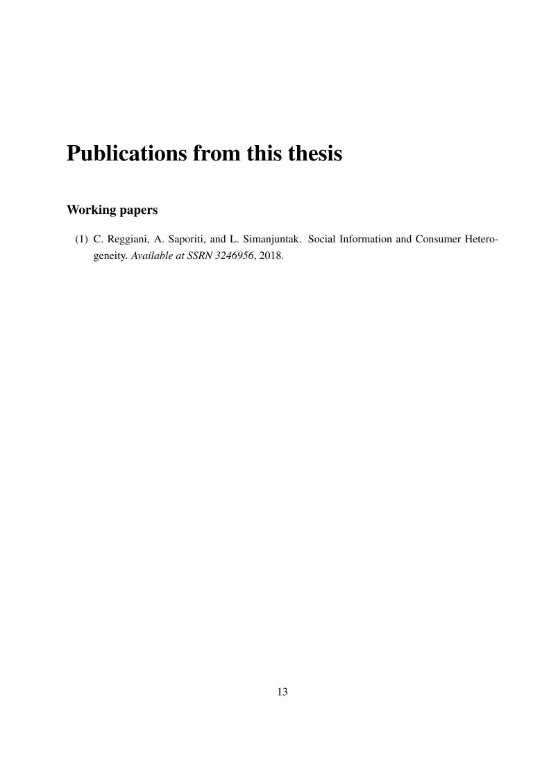
The analyses in Chapters 2 and 4 similarly indicate the significance of consumer heterogeneityon information diffusion (observation) and welfare, as specified in Table 1.1. In Chapter 2, het-erogeneity in responsiveness to advertising allows for a maximum diffusion of information andsubsequently a welfare-maximising equilibrium. Chapter 4 shows that when consumers have dif-ferent valuations of the product, price discrimination is feasible for the firm and it may induce astrictly positive expected consumer surplus.

Table 1.1: Role of consumer heterogeneity revealed in the thesis

Aspect Chapter 2 Chapter 4Type of heterogeneity in responsiveness to advertising in valuation of good

Results withoutno diffusion no observation

of social information of information

heterogeneity social welfare is expected consumer surplus

not maximised is always zero

Results withpossible (maximum) diffusion possible observation

of social information of information

heterogeneity social welfare expected consumer surplus

can be maximised can be strictly positive

In the second chapter, information diffusion (observation) benefits consumers. A social plannerthat maximises expected social welfare shall emphasise to advertising firms the fact that consumersmay be heterogeneous in their responsiveness to advertising and the ensuing potential profitabilityof social information, i.e., how social information can complement advertising, as it can reach lessresponsive ones through more responsive predecessors. This approach will incentivise firms tospend on advertising and warrant information diffusion by the platform.

The work in Chapter 4 suggests that a social planner may opt for a review system or design,with a certain level of spoiling, that maximises expected consumer surplus through its effect on thefirm’s price schedule. However, the pricing policy that maximises expected ex-ante consumer sur-plus prevents observation of information and thereby hinders learning. In this case, the consumercan end up buying the bad-quality product and have a negative realised ex-post utility.

1.2. ORGANISATION OF THESIS 17

1.2 Organisation of thesis

The thesis is divided into five chapters, with the summary given as follows:

Chapter 2: Social information and consumer heterogeneity

This chapter introduces a game of advertising and social information with the focus on studyingthe incentives of a social network to control two types of information circulating on its platform:(i) display advertising by two quality-differentiated firms, and (ii) “social information” (i.e.,purchasing decisions shared among consumers). Consumers engage in a sequential search andtheir choices are influenced by both of these communication channels, whereas the network getsrevenue only through advertising. The equilibrium network diffusion of social information and thefirms’ expenditures on advertising are characterised, and it includes a maximum diffusion levelwhich involves observation of information by every consumer in the latter group. It is shown thatdepending on consumers’ heterogeneous response to advertising, social information can eithercompete with, or be complement of, display advertising. Moreover, in every equilibrium eachconsumer purchases the superior product with a strictly higher probability, and receiving socialinformation further increases such probability. Finally, social information raises social welfare,thereby establishing the existence of a welfare-maximising equilibrium.

Chapter 3: Social information and consumer heterogeneity: Extensions

In this chapter, extensions to the model in Chapter 2 are considered and analysed. These includeextensions to the number of advertising expenditures chosen by firms, the number of consumergroups, the range of the level of responsiveness to advertising, and the sampling procedure.

Chapter 4: Rational spoiling through reviews

This chapter introduces a model of pricing of experience goods that have narrative attributes, withreviews for such products possibly containing “spoilers” that affect consumers’ enjoyment andconsequently influence their purchasing decisions. The objective of the study is to analyse theeffect of the risk of the product being spoiled by a review on a monopolist’s optimal pricing policyand on expected consumer surplus. The results show that consumer heterogeneity in valuationplays a role in the analysis as it allows for price discrimination strategies that would generateinformation and may lead to learning of quality. Furthermore, they indicate the notion of rationalspoiling: if consumers are able to determine the review system, they may strategically commit

18 CHAPTER 1. INTRODUCTION

to one with a sufficiently high risk of spoiling the product for subsequent consumers in order tocounterbalance the potential effect of the firm’s price discrimination over time and make the firmchoose a pricing policy that gives them a higher expected surplus. However, such a policy mayprevent consumers from learning and expose them to the risk of consuming a bad-quality product.

Chapter 5: Concluding remarks

This chapter concludes the thesis with a summary of the main results and possible future researchdirections.

Chapter 2

Social information and consumerheterogeneity

2.1 Introduction

Online social networks has become increasingly popular. As of 2018, there are 3.2 billionpeople using social media, which is forty two percent of the total population on the planet, upthirteen percent from 2017. Internet users are also spending more time on social media. Every daythe average user spends two hours and fifteen minutes on them, accounting for one out of everythree minutes spent online.

Social media networks like Facebook, YouTube, Instagram, LinkedIn, and Twitter are mostly“free” for their users.1 Because of that, online advertising is a major source of income and acharacterising element of the business model of these platforms. Social media advertising is onthe rise and networks are always looking for new advertising spaces in their websites and mobileapps.2 These sponsored messages aim to attract the attention of users to the products or servicesof their client firms.

Online advertising, however, is not the only tool that may raise users’ awareness of productsor services. Social network users, in fact, produce and share a huge amount of material.3 Increating this mass of content, users may also endorse brands and share purchase choices with theirsocial network’s contacts. In other words, the “social information” circulating on a network may

1Facebook notoriously states on its initial page “It’s free and it will always be”.2The forecast advertising revenue of social media for 2018 is about 51.3 billion USD, with an expected annual

growth rate of 10.5 percent in the coming years, and it is predicted to almost double by 2023. See: https://blog.hootsuite.com/social-media-advertising-stats.

3During every minute of every day of 2014, according to Keen [40], the world’s internet users uploaded 72 hours ofYouTube video, shared 2.46m pieces of Facebook content, published 277,000 tweets, and posted 216,000 new photoson Instagram, and these figures are likely to increase year after year.

19

https://blog.hootsuite.com/social-media-advertising-stats

https://blog.hootsuite.com/social-media-advertising-stats

20 CHAPTER 2. SOCIAL INFORMATION AND CONSUMER HETEROGENEITY

influence potential consumers in a way that is similar to advertising.

Importantly, social network users are likely to be heterogeneous in their reaction to each typeof message. Marketing research suggests that millennials tend to be more influenced by socialinformation and less responsive to canonical advertising.4 With the goal of amplifying the impactof online advertising on users, of attracting more advertisers, and of capturing a larger share of themarketing budgets, social networks employ sophisticated algorithms that try to control and orientthe flow of “social information” circulating on their platforms.

This work studies the effects of consumer heterogeneity over the incentives of a social networkto control two types of information circulating on its online platform: (i) display advertising, whichconsists of banners and other messages of uninformative content (such as text, images, flash, video,and audio) sent directly to the network users (consumers) by the advertisers (firms), and (ii) social

information, which takes the form of previous purchasing decisions shared among the consumersthemselves on the network.

The model considered in this chapter focuses on an online social network connecting a contin-uum of consumers and two firms that sell quality-differentiated products. Consumers wish to buythe high quality product, but the quality of each good is privately observed by the sellers. Con-sumers can uncover quality before buying by engaging in to a costly and sequential sampling ofthe goods. Some examples of such kind of sampling include clicking on the banner or link that re-directs the consumer to the firm’s web page, checking product specifications, opening comparisonweb-sites, reading reviews, or watching unboxing videos. In the model, diverse search costs reflectindividuals’ differences in their willingness to engage in these activities.

The network maximises the firms’ expenditures on display advertising. The main purpose ofdisplay advertising is to raise product awareness and increase the purchase intentions of consumers,but it is uninformative of the product quality. To be more precise, each firm uses its online adver-tisement to persuade the consumers to sample its product first. Besides sampling costs, consumersare also heterogeneous in their responsiveness to advertising, i.e., in the probability to be persuadedto sample a particular product.

Consumers do not buy the product all at the same time. There is a mass of “early consumers”that buy the product first, and a mass of “late consumers” that shop afterwards. Besides samplingand shopping first, the early consumers observe on the network only display advertising, whereaseach member of the late group, in addition to an advertisement, may independently observe on-line an early consumer’s purchase. The probability of observing such information is strategicallydetermined by the platform, and is referred to as the network diffusion of social information. Thepurchases of the early group provide a noisy signal about the quality of the products. The noise

4Newman, D. Research Shows Millennials Don’t Respond To Ads. Forbes, April 28, 2015. https://www.forbes.com/sites/danielnewman/2015/04/28/research-shows-millennials-dont-respond-to-ads/.

https://www.forbes.com/sites/danielnewman/2015/04/28/research-shows-millennials-dont-respond-to-ads/

https://www.forbes.com/sites/danielnewman/2015/04/28/research-shows-millennials-dont-respond-to-ads/

2.2. RELATED LITERATURE 21

results because the late consumers do not know for sure if the early consumers have sampled oneor both products, given the uncertainty about the individual costs of sampling (searching).

The main results of the chapter are as follows. First, the chapter characterises the equilibriumlevel of diffusion of social information and the firms’ advertising expenditures. Second, it showsthat social information can either compete with, or be complement of, display advertising. Third,the nature of the relationship between these two ways of reaching consumers on the platform isshown to depend mainly on their heterogeneous response to advertising.

To elaborate, when consumers are equally responsive to advertising, display advertisementsand social information compete with each other. In this case, the platform sets in equilibrium theminimum diffusion and shuts down social information to encourage firms’ spending on advertising.By contrast, when consumers react differently to advertising, the two information channels can becomplements. For that to happen, display advertising directly influences the more-responsive earlyconsumers, whereas the transmission of their purchase decisions (social information) indirectlycaptures the late consumers, who are less responsive to advertising and are more likely to emulatetheir predecessors. In this case, the platform sets in equilibrium the maximum level of diffusion.

Fourth, the chapter proves that in every equilibrium each consumer almost surely purchasesthe superior product with a strictly higher probability, and that receiving social information almost

surely further increases the probability of buying such product. Finally, fifth, social informationis shown to almost surely increase social welfare, establishing as a by-product the existence ofa welfare-maximising equilibrium. These results confirm that in the current environment socialinformation is informative and valuable.

The rest of the chapter is organised as follows. A review of related literature is given in Sec-tion 2.2. Section 2.3 describes the framework, including firms, consumers, and the online socialnetwork. The main results are presented in Section 2.4. Section 2.5 concludes. For expositionalconvenience, all proofs are in Appendix A.

2.2 Related literature

Regarding the literature more closely related with the current chapter, there is first a stream of workthat focuses on platforms as intermediaries, which can strategically distort the content providedby different sides to achieve revenue maximisation. To mention a few examples of this literature,biased news has been studied by Reuter and Zitzewitz [61] and Ellman and Germano [28]; whereasbiased search has been analysed in Burguet, Caminal, and Ellman [17] and de Corniere and Taylor[24], among others. The social network in this chapter acts in a similar fashion, manipulatinginformation diffusion on its platform to maximise display advertising spending.


Second, there is a rapidly growing literature on consumer search. Sequential search of differentproducts was pioneered by Weitzman [68] and recently used, inter alios, by Armstrong, Vickets,and Zhou [3] and Armstrong and Zhou [4] in studying prominence in search. In this chapter’smodel, display advertising leads to prominence, by making a firm’s product more visible to con-sumers. Sequential search and observational learning by agents, important elements of the setupstudied in this chapter, are analysed more in depth in Mueller-Frank and Pai [50] and Garcia andShelegia [34].

Third, the literature on advertising has highlighted the role of sponsored messages as targetedand informative advertising.5 In this chapter, online display advertising by competing firms hasthe sole objective of raising awareness. In particular, to increase the chances to be clicked, firmsbid in an all-pay advertising auction, as developed by Friedman [29], and more recently used inBimpikis, Ozdaglar, and Yildiz [14] and Dockner and Jørgensen [25]. However, unlike the modelof Friedman [29] in which two firms have equal price, quality, reputation, and service, the marketin this chapter is a differentiated duopoly, as in Gabszewicz and Thisse [30]. In such an industry,quality is exogenously given as one firm produce a high-quality product and the other produce alow-quality (“standard”) product, and the two are more or less close substitutes for each other.

Additionally, price is supposedly exogenous in this chapter. The product being sold is a searchgood, meaning that its quality is only known upon sampling. Thus, it could be argued that con-sumers perceive firms as having equal quality before they do any search. The two firms competein advertising that may persuade consumers to sample first their product and disclose its quality,and they would need to set the same price in order to be competitive. In this regard, there is nosignalling of quality and advertising is the only factor that influences the first sampling decisions.In the differentiated industry setting of Gabszewicz and Thisse [30, 31], products are of differentquality but the unit cost of producing either is the same and assumed to be zero. Therefore, itis reasonable to expect firms to have equal (exogenous) price. Moreover, it can assumed that thehigh-quality firm already knows that it has the advantage of being purchased by every consumerwho samples twice due to having the better product. This fraction of consumers are guaranteedeven without having to signal its high quality with (a higher) price.

Finally, this chapter also relates to the literature on information transmission in social net-works. People are influenced by friends’ opinions in deciding which products to buy (Jackson[37]). They can also infer quality from the choices of others and/or acquire more information frompeers (Kircher & Postlewaite [41]). Mueller-Frank and Pai [49], the most closely related articleto this chapter, shows that an online social network (platform) has an incentive to block socialinformation in order to increase advertising revenue. Building upon the latter, the current workextends Mueller-Frank and Pai [49] by focusing on the effects over social information diffusion

5See, e.g., Bagwell [6], Renault [60], Choi, Mela, Balseiro, and Leary [22] for reviews.

2.3. SETUP 23

of consumers’ heterogeneous responsiveness to advertising. In particular, the chapter shows thatMueller-Frank and Pai’s main result of no transmission arises only as a special case when earlyand late consumers are equally responsive to advertising.

Consumers have the same level of responsiveness to advertising, i.e., the probability of sam-pling first the advertised product, in Mueller-Frank and Pai [49]. In this respect, social informationalways compete with display advertising as it is an alternative information source which rendersthe advertisements ineffective and one that does not give any direct revenue to the platform. Themodel in this chapter, meanwhile, allows for heterogeneous levels of responsiveness to advertisingacross individuals and groups. This heterogeneity makes it possible for social information to com-plement advertising: a relatively unresponsive (late) group of consumers can be reached via a moreresponsive (early) group. In other words, social information may indirectly benefit the platform asit can make display advertising more compelling and the firms’ spending on it worthwhile.

In Mueller-Frank and Pai [49], the online social network may permit circulation of sponsored

social information, which diffusion level depends on how much firms pay. Nevertheless, organic

social information is always shut off; that is, social information is valuable for the platform onlywhen it provides direct revenue. The research in this chapter notably shows that it is possible toinduce the organic relay of social information by simply introducing consumer heterogeneity inresponsiveness to advertising, without the existence of sponsored social information.

2.3 Setup

Consider a market with two firms, indexed by i = A, B, who sell (at an exogenous price) a goodof quality qi ∈ [0,1], where q = min{qA,qB} (and respectively, q = max{qA,qB}) denotes thelowest (and respectively, highest) realised product quality. There is a continuum of consumersin the market divided into two groups G = E, L, referred to as the early and the late consumers,with typical elements denoted by e ∈ E and ` ∈ L, respectively. The mass of early consumers isnormalized to 1, and the (relative) mass of late consumers to λ > 0.

To raise awareness of their products and maximise their sales (i.e., the number of units sold),the firms invest on display advertising (also known as banner advertising) in a social network (plat-form). The network maximises the advertising expenditures of the firms by setting the diffusionv ∈ [0,1] of information on the platform, which determines the probability that any late consumerindependently observes the purchasing decision of an early consumer.

Both groups of consumers prefer the product with the highest quality. However, good qualityis unobservable to the consumers. The early consumers shop first and carry out a costly sequentialsearch; sampling a product perfectly reveals its quality. Consumers can sample either one or bothproducts, before buying a single unit from one of the firms. The late consumers do the same


afterwards. In addition to sampling, the late consumers might also receive social informationcirculating on the network, which consists of the purchases of the early consumers. The utility ofeach consumer is the quality of the purchased product minus the search cost.

Let α j be the probability that consumer j ∈ G samples first the product that she observes onthe advertising banner. The parameter α j is interpreted as the responsiveness to advertising ofconsumer j’s sampling decisions. That is, α j reflects how influencaable and easy to persuadeis j ∈ G by the firms’ advertising strategies. This persuasion parameter is heterogeneous acrossindividuals and groups. The firms and the network only know the mean values of α j within eachgroup G = E,L but not the exact value of α j for each consumer j ∈ G. In the sequel, it is assumedthat for each group G = E,L and every consumer j ∈ G, α j is independently drawn from a group-specific cumulative distribution function (c.d.f.) on [0,1] with mean values αG > 1/2, and that it isprivately observed by individual j.6

The game of advertising and social information sketched above consists of the followingsequence of events:

Period 0: The platform sets the diffusion v ∈ [0,1] of the network. The quality qi of firm i is inde-pendently drawn from a c.d.f. Fq on [0,1], with probability density fq positive everywhere.The firms observe the realised qualities (qA, qB), c.d.f. Fc of consumers’ search cost, andmean values αE , αL of consumer groups’ responsiveness to advertising. They simultane-ously and independently choose the expenditures mi ∈ [0,M] on display advertising, whereM > 0 is a large positive integer. The probability that a consumer j ∈G independently sees abanner for product A, (and respectively, B) is given by the expenditure ratio ρ = mA

mA+mB (andrespectively, 1−ρ).

Period 1: For each early consumer e ∈ E, her search cost Ce is drawn from a c.d.f. Fc on [0,1],with density fc positive everywhere. Each early consumer e observes αe and Ce, and withprobability ρ (and resp., 1−ρ) she sees a banner θe = A (and resp., θe = B) of one of thefirms. She subsequently samples at no cost θe with probability αe, and the other product withprobability 1−αe. Sampling the remaining good is possible, but with a cost given by Ce.The quality qset of the sampled products is immediately revealed, where set ∈ {A, B} denotesthe sample choices of e ∈ E, with t = 1, 1′ representing her two trials. The early consumere ∈ E buys the sampled product with the highest quality, with ae ∈ {set}t=1,1′ indicating herconsumption choice.

6The fact that αG > 1/2 simply means that on average both groups sample first more frequently the product thatappears on the ad. The main results do not rely on this assumption, and they extend easily to the case where either αEor αL are below half, which is presented in Section 3.2.

2.4. RESULTS 25

Period 2: Each late consumer ` ∈ L engages into the same shopping routine as that of the earlyconsumers, with α`, C`, θ`, s`t , qs`t , and a` redefined accordingly. The difference betweenthe groups is that before deciding which product to sample first, with probability v consumer` observes a purchasing decision ae, which is randomly selected with equal probability fromthe set of the early consumers’ purchased goods.

An equilibrium of the game of advertising and social information is a perfect Bayesian Nashequilibrium in pure strategies.

2.4 Results

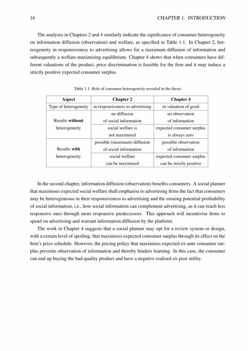
Let N ⊆ E ∪L represent the group of (early and late) consumers who only observe display adver-tising, and let O⊆ L be the set of late consumers who observe social information in addition to theadvertisement. Note that a consumer j ∈ N that samples first a product of quality qi will sample asecond good if and only if the expected quality gain (according to j’s prior belief) from the secondtrial is above j’s search cost C j; that is,

∫ 1

qi(q−qi)dFq(q)≥C j. (2.1)

Denote by IN(qi) =∫ 1

qi (q−qi)dFq(q) the cut-off cost that makes individual j ∈ N indifferent be-tween searching once or twice, given that the quality of the product sampled first is qi. The prob-ability that j ∈ N searches only once (buys the first product sampled i) is τN(qi) = 1−Fc(IN(qi)).For notational convenience, denote τN(q) = τN .

Likewise, a consumer j ∈O⊆ L that observes a purchase ae = i of quality qi reckons that either:(1) the early consumer e could have sampled only ae, which provides no valuable information, or(2) e could have sampled both A and B, in which case ae must be the highest quality good. Thus,individual j’s posterior belief is that ae dominates (quality wise) the other product, and that is whatj samples first.7 Further, consumer j ∈ O will sample a second good if and only if,

τN(qi) ·∫ 1

qi(q−qi)dFq(q)≥C j, (2.2)

7Specifically, sampling first ae = i strictly first-order stochastically dominates sampling the other product−i: givenany q ∈ (0,1) and a consumer’s prior belief on any first sampling P(qs j1 ≥ q), her posterior belief on sampling i isP′(qi ≥ q) = P(qi ≥ q | ae = i) = τN(qi)P(qs j1 ≥ q)+

(1− τN(qi)

)> P(qs j1 ≥ q), whereas the posterior belief on −i

is the same as the prior and therefore P′(qi ≥ q)> P′(q−i ≥ q). Consequently, E[qi | ae = i] =(1−P′(qi ≥ q)

)·E[qi |

qi ≤ q] +P′(qi ≥ q) ·E[qi | qi ≥ q] > E[q−i | q−i ≥ q] +P′(q−i ≥ q) ·(E[q−i | q−i ≥ q]−E[q−i | q−i ≤ q]

)= E[q−i].

That is, an informed consumer has a higher expected utility from sampling first the observed purchase ae = i.


where the left-hand side of (2.2) is j’s expected quality gain from her second trial (according toher posterior belief). As before, define by IO(qi) and τO(qi), respectively, the cut-off cost and theprobability of stopping search after the first sampling for the (socially) informed late consumers,with τO(q) = τO. It is immediate from the inequalities (2.1) and (2.2) that IO(qi) < IN(qi) for allqi ∈ [0,1], and consequently that τO(qi)> τN(qi).8

Before consumers search, both firms observe qualities qA and qB. The low-quality firm withq = min{qA,qB} is disadvantaged because any consumer who samples twice will purchase thehigh-quality product from its competitor. As the only consumers who will buy the inferior goodare those who sample first q and stop searching. As a result, the low-quality firm’s potential con-sumers consist of a fraction τN of the uninformed group, who can be influenced directly throughadvertising, and a fraction τO of the informed group, who are reached indirectly through the τN

fraction of the early group. The high-quality firm is guaranteed the fraction of consumers whosearch twice, hence these non-searching potential consumers are the only ones for which advertis-ing competition takes place.

Given the responsiveness to advertising αG of each group G ∈ {E,L}, its mean sample biastowards advertising is αG− 1/2; this bias expresses how much more likely a consumer in G is tosample first the advertised product rather than the unadvertised one. If a late consumer does notreceive social information, her first sampling depends on her own response to the advertising andit will be converted into a purchase with probability τN , which is the likelihood that she will stopto buy the initially searched good. As such, an uninformed late consumer’s effective response toadvertising is given by τN · (αL− 1/2).

When there is diffusion of social information, advertising influences the informed late con-sumers indirectly through the persuasion exerted on them by the early group’s purchases and theirfirst sampling decisions are subject to the responsiveness (bias) of the early consumers instead. Theconversion of advertising bias to a purchase requires both the informed late consumer and the un-informed early consumer she observes to sample only once, which happens with probability τN τO.Accordingly, the informed late consumer’s effective response to advertising is τN τO · (αE − 1/2).

The following function h can then be defined, which yields the difference between the tworesponses and plays a key role in the subsequent analysis:

h(αE , αL,τO) =

(αL−

12

)− τO ·

(αE −

12

). (2.3)

The function h(αE , αL,τO) captures the consumer heterogeneous response to advertising due tothe presence of social information. When h(·) > 0 (and resp., h(·) < 0), the effective bias of the

8Notice that IO(qi) and IN(qi) may be equal if τN(qi) = 1, which requires qi = 1. However, given that fq iswell-defined and is positive everywhere on the support [0,1], qi 6= 1 almost surely.

2.4. RESULTS 27

uninformed (and resp., informed) late consumers is higher: it is therefore more effective to reachthem through direct (and resp., indirect) advertising and social information competes with (andresp., complement) banner advertisements as an instrument of persuasion for the firms. Instead,when h(·) = 0, both display advertising, social information, and any mixture of them are equallyeffective to reach the platform’s users.

The following proposition characterises the equilibrium strategies of the platform and the firms,for the different regions determined by h(αE , αL,τO).

Proposition 1 (Equilibrium characterisation) The equilibria of the advertising and social in-

formation game are such that the expenditures on display advertising are strictly positive and the

same for both firms, i.e., mA = mB(= m)> 0, and

(i) v = 0 and m = 12 τN

[(αE − 1

2

)+λ

(αL− 1

2

)], if h(αE , αL,τO)> 0;

(ii) v ∈ [0,1] and m = 12 τN

[(αE − 1

2

)+λ

(αL− 1

2

)], if h(αE , αL,τO) = 0; and

(iii) v = 1 and m = 12 τN

(αE − 1

2

)(1+λτO), if h(αE , αL,τO)< 0.

It is clear from Proposition 1 that, except in the knife-edge case (ii) where any level of networkdiffusion is optimal, the equilibrium of the game is unique.

Corollary 1 (Uniqueness) If h(αE , αL,τO) 6= 0, then the advertising and social information game

has a unique equilibrium.

The different levels of diffusion of social information, v, emerging from equilibria of type (i)-(iii) described in Proposition 1 are illustrated in Figure 2.1. These levels depend on the positionof the locus h = 0. To elaborate, suppose that the responsiveness to advertising αL of the averagelate consumer is relatively low, meaning that it lies below the upward-sloping dashed line (h < 0).In this case, social information is from the firms’ viewpoint more effective to exert influence onthe group. The network is aware of this, and it maximises the firms’ expenditures by linking theearly consumers’ shopping decisions to the sampling behavior of the late group, allowing socialinformation to circulate freely on the platform (v = 1). The unique equilibrium is consequentlylocated on the grey-shaded region on Figure 2.1.

By contrast, when αL is above the dashed line (h > 0), the late consumers are relatively moreresponsive as a group to advertising. This means that the firms can persuade this group moreeffectively by reaching them directly with the banners, without relying on the flow of social infor-mation. That offers little incentives to the platform to allow a high level of connection betweenthe purchases of both groups. In fact, the only type of equilibrium consists of the cross-shadedregion on Figure 2.1, where the information diffusion is v = 0. The situation illustrated by the


red-shaded area (on h = 0), that is, the second type of equilibria, is a knife-edge case where anylevel of diffusion v ∈ [0,1] will do as well.

Figure 2.1: Illustration of areas of the three types of equilibrium (Proposition 1)

The next corollary displays as a special case of Proposition 1 the equilibrium when αE = αL,showing that it can only be of type (i): as the mean sample bias towards advertising is the samefor both groups, the effective response of informed late consumers is smaller by a fraction τO andtherefore h > 0. Figure 2.1 exhibits the result on the blue-shaded region, which arises from theintersection between the 45-degree line and the cross-shaded area. In equilibrium, the networkdoes not allow social information to circulate on its platform.

Corollary 2 (Mueller-Frank and Pai [49]) If αE = αL = α, then the equilibria of the adver-

tising and social information game are such that the firms’ expenditures are mA = mB =12 τN

(α− 1

2

)(1+λ), and the network diffusion is v = 0.

When consumers have the same responsiveness level to advertising or all consumer groups areequally responsive on average, as in Mueller-Frank and Pai [49], the platform always shuts offthe organic relay of social information as it competes with display advertisements and thereforedisincentivises spending on advertising. The referred paper shows that the platform may, however,allow sponsored social information–purchase decisions that firms pay the network to display tolate consumers–which gives it direct revenue. The work in this chapter suggests that a non-zerodiffusion of (organic) social information is achievable by simply introducing heterogeneity in con-sumers’ responsiveness to advertising, even without the existence of sponsored social information.

2.4. RESULTS 29

Given this heterogeneity, organically circulated social information potentially complements adver-tising through its role in reaching a less responsive late group via relatively more responsive earlyconsumers; that is, when (αE , αL) is in the grey-shaded region on Figure 2.1. This complementar-ity increases the appeal of investing on advertisements and thus benefits the platform indirectly.

Notice that on Figure 2.1 the size of the equilibrium regions depends on the value of τO, whichis the probability of an informed late consumer sampling only once. When τO is relatively large,the group does not expect much gain from a second trial, even after updating their beliefs withsocial information. As a result, it becomes more likely that the informed late consumers willemulate the early consumer they observe. A greater τO rises therefore the effective response ofthe late group to advertising, by discouraging the informed subgroup to sample more than once.This shifts upwards the locus h(·) on Figure 2.1, and it expands the type (iii) equilibrium region,where social information circulates freely. When τO is relatively small, instead, the locus shiftsdownwards and the type (i) region is enlarged.

With regard to the firms’ expenditures on advertising, Proposition 1 indicates that they arepositive and identical for both firms, independent of the quality of their goods. That is, none ofthe firms (in particular, the high-quality firm) finds it beneficial to signal product quality to theconsumers by spending more on advertising. The reason is because consumers do not observethe firms’ expenditures, but only a single banner with a certain probability. As they do not knowthe frequency with which the banner is realised, they cannot infer quality by simply observing it.That is, there is no way of truncating the distribution of quality after being exposed to a displayadvertisement. This implies that regardless of the quality of their products, both firms face exactlythe same incentives (represented in Appendix A.1 by the first-order conditions (A.3) and (A.4)) toinvest on advertising.

The closed-form expression for the equilibrium expenditures in Proposition 1 offers the possi-bility of analysing how display advertising varies with respect to the main parameters of the model,namely, p = (v, αE , αL,λ,τO,τN ,q). The next proposition collects these results.

Proposition 2 (Comparative statics) Let m(p) denote the equilibrium expenditures of the firms

in the advertising and social information game. Regardless of the network diffusion v ∈ [0,1],∂m(p)

∂p ≥ 0 for each parameter p = αE , αL,λ,τN ,τO,q.

In accordance with intuition, the above proposition confirms that at the equilibrium the firms’advertising expenditures are increasing in the groups’ responsiveness to advertising, the fractionof late consumers, the probabilities of sampling only once, and the lowest realised product quality.As to the comparison of m for different values of the network diffusion v, the results are am-biguous. Equation (A.6) in Appendix A.1 shows that the sign of ∂m/∂v coincides with the sign of


−h(αE , αL,τO). Moreover, the expenditures can be higher in either type of equilibrium dependingmainly on the different values of αE , αL and τO.

Turning to the consumer behavior, Appendix A.3 shows that in every equilibrium of Proposi-tion 1, each consumer j ∈N who does not receive social information purchases the inferior productwith probability 1

2 τN , which is the probability of observing the inferior good on the ad and buyingthe first product sampled. Similarly, each consumer j ∈ O who receives social information buysthe inferior product with probability 1

2 τN τO, which is the probability that the early consumer buysthe inferior good times the probability that the late consumer samples only once. Thus, putting thistogether, it transpires that:

Proposition 3 (Consumer behaviour) In every equilibrium of Proposition 1, (1) each consumer

almost surely purchases the superior product with a strictly higher probability, and (2) receiving

social information almost surely further increases the probability of buying the superior product.

So far, the level of expenditures mi is assumed to be in the interval [0,M], where M > 0 is alarge positive integer. In fact, the expenditures must be sufficiently small for the firms to participateor compete in advertising. The following proposition confirms that this is indeed the case in anyof the equilibrium characterised in Proposition 1.

Proposition 4 (Firm profit) In every equilibrium of Proposition 1, both firms have strictly posi-

tive profits and the firm with the superior product has a strictly higher expected profit than the firm

with the inferior product, i.e.,

Π > Π > 0.

Moreover, in any equilibrium of type (ii) in Proposition 1, the high-quality firm prefers a higher

network diffusion while the low-quality firm prefers a lower diffusion, i.e.,

∂Π

∂v> 0 and

∂Π

∂v< 0.

The first part of the proposition indicates that participation constraints for both firms are satis-fied. In particular, it tells us that though the firms have strictly positive expected profits in equilib-rium, the level of profits differ. That is, the firms’ equal advertising expenditures (Prop. 1) do notresult in equal profits. The difference in product quality may explain this outcome: a consumerbuys the inferior product only when she samples first this product and does not search further; inevery other case she would purchase the superior product. So when both firms spend the sameamount on advertising, as in every equilibrium, intuitively the high-quality firm have a higherchance of selling its product and a higher level of profit than the low-quality firm.

2.4. RESULTS 31

In a type (ii) equilibrium, the platform sets any v ∈ [0,1] since its revenue does not change withthe level of network diffusion. The second part of Proposition 4 shows that the diffusion, however,affects the firms’ level of profits. In every equilibrium, a late consumer has a higher probabilityof purchasing the inferior product when she does not observe any social information. Therefore arise in diffusion level would lower the profits of the low-quality firm and accordingly benefits thehigh-quality firm. Furthermore, it can be inferred that social information helps each late consumergain a higher utility from consuming the superior product. It is then reasonable to predict that anincreased diffusion of information would improve social welfare.

In light of these results, an interesting question to ask is whether social information increasessociety’s well-being. To answer this question, define the ex-ante (expected) social welfare W (·) inthe following way:

W (v) = ∑mi

︸︷︷︸network

+(1+λ−∑mi)︸︷︷︸

firms

+ 1 ·E(qae−Ce)︸︷︷︸early consumers

+

+λ · [v ·E(qa`−C` | ` ∈ O)+(1− v) ·E(qa`−C` | ` ∈ N∩L)]︸︷︷︸late consumers

,(2.4)

where E(·) denotes the expectation operator.

Notice that the revenue of the network ∑mi is equal to the firms’ expenditures on displayadvertising. In addition, the well-being of the early consumers E(qae−Ce) is not affected by socialinformation. Thus, rewriting (2.4) as

W (v) = 1+λ+E(qae−Ce)+λ · E(qa`−C` | ` ∈ N∩L)+

+ v ·λ · [E(qa`−C` | ` ∈ O)−E(qa`−C` | ` ∈ N∩L)] ,(2.5)

it becomes apparent the social information diffusion v only features in the last term of the right-hand side of equation (2.5). Hence, the efficiency of the three types of equilibria described inProposition 1 depends on how the diffusion of the platform interacts with the difference between(a) the expected welfare (quality gain over the search cost) of the late consumers that observe thepurchases of the early group, and (b) the expected welfare of those in the late group that decidewhich product to buy based solely on advertising information.

The next proposition points out that for the equilibrium of the advertising and social informa-tion game to maximize social welfare, the late consumers must be able to observe with certaintythe purchases of the early group.

Proposition 5 (Social welfare) In every equilibrium of Proposition 1, social welfare is almost

surely strictly increasing in the network diffusion, i.e., ∂W (v)∂v > 0. Therefore, arg max

v∈[0,1]W (v) = 1.


An immediate implication of the above proposition is that only types (ii) and (iii) are welfare-maximising equilibria. This happens because social information is valuable for consumers. Thereis a positive probability that an arbitrary early consumer has sampled both products, and thereforethat the observed purchase, which is the first good sampled by the late consumers, has the bestquality. Thus, any late consumer has a higher probability of purchasing the superior product ifshe receives social information. Moreover, as the late consumers are able to update their beliefson quality with the information observed from the early group, their cut-off cost is lower and,consequently, they spend less on search.

2.5 Concluding remarks

This chapter studies the incentives of an online social network to control two kinds of data circulat-ing on its platform: display advertisement and social information. Online social networks accruerevenues through advertising and their users are potential buyers of the advertised products. Socialinformation is produced by users posting on the network and it may be useful to other consumers.As such sharing may include purchase choices, online social information potentially competeswith conventional advertising in raising consumers’ awareness, and its flow can be controlled bythe social network.

In this context, the chapter builds upon a platform model in which an online social networkconnects firms and consumers. The products of the two firms are quality differentiated. Firms caninvest in advertising but such expenditure cannot signal quality. In addition to having differentsearch costs and time of purchase (early or late), consumers are also heterogeneous in the level ofresponsiveness to advertising. The work in this chapter emphasises the role of such heterogeneityin determining the relationship between advertisement and the flow of social information, and howthe latter can be distorted by the platform as a result.

In particular, the findings suggest that if early and late consumers are, on average, fairly ho-mogeneous in their responsiveness to advertising, then social information simply competes withdisplay advertising. Heterogeneity, instead, can lead to a complementary relation between the twoinformation channels. That is, advertising reaches the more-responsive early group of consumersand social information then relays their purchase decisions to the less receptive late group. Hence,firms do invest in advertising, despite social information also circulating on the platform. More-over, in this chapter social information is valuable to consumers and welfare is maximised whenfull diffusion is allowed.

For sake of clarity, a rather stylised model of social networks is employed, but one that canbe potentially extended in several directions. Whereas the monopoly assumption is justifiablein situations with strong network effects or widespread multi-homing, the model may include

2.5. CONCLUDING REMARKS 33

multiple platforms. Competition between these platforms may affect the incentives to manipulateinformation, as in Ellman and Germano [28]. Further, the model is restricted to two groups ofconsumers. Unlike the extreme levels of diffusion in the equilibria, introducing more groups maygenerate interior solutions in which the platform chooses some optimal level of social information–this is revealed to be the case in Section 3.1. Finally, in the search model consumers can only buya product that they have sampled. Following Doval [26], this assumption could be relaxed, as isdone in Section 3.4.

Chapter 3

Social information and consumerheterogeneity: extensions

The following extensions relaxed some of the assumptions made in the stylised model of Chapter2 to better reflect what is potentially seen in practice.

First of all, Proposition 1 and Corollary 1 in Chapter 2 reveal that in any unique equilibriumof the game, the platform sets diffusion level v = 0 or v = 1. This all-or-nothing approach israrely the case in reality, as social networks regularly moderate content and filter information ontheir platforms to a certain degree. A likely reason for the binary choice is the fact that there areonly two consumer groups and the comparison between their responsiveness determines whetherinformation diffusion is lucrative to the platform (represented by the sign of ∂m/∂v). Assumingthat information diffusion is not adjusted throughout time, adding a third group would involveconsideration of three responsiveness levels and may lead to a unique equilibrium with a moderatediffusion v∗ ∈ (0,1). This hypothesis is confirmed by the work in Section 3.1, which also yieldsthe additional result that being informed in a later group is better for consumers as it increases theprobability of buying the superior product.

Secondly, the initial model assumes that αG > 1/2 for each consumer group G; that is, onaverage, consumers are responsive to advertising or biased towards the advertised product. Real-istically, this might not be the case: consumers may experience some disutility from exposure toadvertising or have some negative perceptions on firms who (need to) advertise. The extension inSection 3.2 suggests that most of the derived results remain the same, apart from the equilibriumcharacterisation: now, advertising can still benefit firms, with or without social information, evenif one out of the two groups has an average responsiveness level that is lower than or equal to 1/2.

Thirdly, the each firm in the model presumably makes a one-time investment in advertisingthat will influence both consumer groups. In practice, firms may choose to target a certain group,

34

3.1. EXTENSION TO GROUPS OF CONSUMERS 35

i.e., put more focus on swaying either the early or the late group given their responsiveness to ad-vertising, so that the investment will be more cost-effective. In the extended model in Section 3.3,firms decide an advertising expenditure amount for each period t = 1,2. Similar to the extension inSection 3.2, the equilibrium characterisation result is the sole change but notably firms now investsolely in one period outside the knife-edge case. In the equilibrium with no social information(v = 0), firms do not invest in the first period and choose to target the uninformed late group. Onthe contrary, they do not invest in second period in the equilibrium with maximum informationdiffusion (v = 1) as they are fixated on the early consumers, who help them reach the late groupvia their purchase decisions.

The fourth extension done in Section 3.4 produces several results that significantly deviatesfrom those in the initial model, in which consumers can only purchase goods they have sampled.This assumption is relaxed in the extended model by allowing consumers to buy a product they didnot inspect when the quality in hand is sufficiently low. ‘Betting’ on the unsampled product can bea cheaper alternative in trying to acquire the superior good as consumers may not need to samplea second time to get better quality.

In this final extended model, firms take into account the expected value of product quality,and how the realised qualities compare to it, when choosing their advertising expenditures. Whenqualities are on either side of the expected quality (lower quality is subpar and higher quality isabove-par), every consumer eventually discovers the superior product, with or without a secondsampling, and the case is fittingly trivial: there is no spending on advertising regardless of infor-mation diffusion. If both qualities are above-par, the model is analogous to that in Chapter 2 andthe initial results are unaffected.

Results are strikingly different when the two qualities are subpar. In this instance, social infor-mation ‘reverses’ the effect of advertising on early consumers: a desired effect on the early group E

turns into an opposite effect on the late group L, and vice versa, an opposite effect on E becomes adesired effect on L. Remarkably, advertising is still worthwhile even if the average responsivenesslevel of both groups is lower than or equal to 1/2. Furthermore, observing social information nowdecreases the probability of buying the superior product and social information has an ambiguouseffect on welfare, i.e., information diffusion may not be welfare-improving.

3.1 Extension to groups of consumers

In the benchmark model in Chapter 2, there are two groups of consumers in the market: the earlygroup and the late group. A consumer in j ∈ G samples first the product that is advertised withprobability α j, and its mean value for each group G = E,L is given by αG, with αG > 1/2. Recall

36CHAPTER 3. SOCIAL INFORMATION AND CONSUMER HETEROGENEITY: EXTENSIONS

that τO denotes an informed consumer’s probability of stopping search after the first sampling, i.e.her probability of buying the product that is sampled first.

The function h(αE , αL,τO) = (αL− 1/2)− τO (αE − 1/2) corresponds to the difference betweenthe effective response to advertising of a consumer in the late group L if she is uninformed (given byτN (αL− 1/2)) and if she is informed (given by τN τO (αE − 1/2)). The equilibrium characterisationdepends on h(αE , αL,τO), and the advertising expenditure in equilibrium is given by

m =12

τN

{(αE −

12

)+λ

(αL−

12

)−λ v h(αE , αL,τO)

}.

For generalisation, denote the early group E as the base uninformed group G0 and the lategroup L as G1, the first group to potentially receive social information. The function

f0,1 =−h(αE , αL,τO) = τO

(α0−

12

)−(

α1−12

)

therefore measures the difference between the effective response of an informed consumer in G1

and that of an uninformed consumer in G1; it signifies the impact of social information on theeffectiveness of advertising. By the proof of Proposition 1, sign(∂m/∂v) = sign( f0,1) and the equi-librium diffusion level v is as illustrated in Figure 3.1, which is simply written as follows:

(i) If −h = f0,1 < 0 then v = 0,

(ii) If −h = f0,1 = 0 then v ∈ [0,1],

(iii) If −h = f0,1 > 0 then v = 1.

α012

1

α1

1

(i) v = 0

(iii) v = 1

f0,1 = 0

(ii)v∈ [0

, 1]

Figure 3.1: Illustration of equilibrium with two consumer groups


Now consider a more general model of M ≥ 2 groups of consumers, M ∈N. Denote the groupsby Gk,k = 0,1, . . . ,M−1, with Gk having mass λk and expected value of responsiveness αk. G0 isthe earliest group that does not receive any social information, and each consumer in a subsequentgroup Gk,k = 1,2, . . . ,M− 1 observes a purchase decision of a consumer in group Gk−1 withprobability v, as depicted in Figure 3.2.

Firm ii = A,B mi

Platform(OSN)

Qualityqi ∈ [0, 1]

Expendituremi ∈ [0,M ]

Profit

= units sold - mi

Diffusionv ∈ [0, 1]

Revenue

= mA+mB

probability

of consumer

seeing banner i

mi

mA+mB

G0 v G1 . . . GM−2 v GM−1

α0 ,

mass λ0

α1 ,

mass λ1

αM−2 ,

mass

λM−2

αM−1 ,

mass

λM−1

Figure 3.2: Illustration of model with M groups

Let αk >12 for all k = 0,1, . . . ,M−1. For k = 1,2, . . . ,M−1, define the function

fk−1,k = f (αk−1, αk,τO) = τO

(αk−1−

12

)−(

αk−12

)(3.1)

which represents the impact of social information on the effective response of a consumer in Gk.This function shall be referred to as the intergroup function between group k− 1 and group k,as it compares the direct effect of advertising on group k (without diffusion of social information,through the responsiveness of the group itself) with the indirect effect of advertising (with diffusionof social information, through the responsiveness of the preceding group k−1) and thus it dependson the responsiveness of both groups.


In the extended game with three consumer groups, the two intergroup functions are given by

f0,1 = τO

(α0−

12

)−(

α1−12

)and f1,2 = τO

(α1−

12

)−(

α2−12

).

The equilibrium is characterised in the following proposition and illustrated in Figure 3.3.

Proposition 6 (Equilibrium characterisation with three consumer groups) The equilibria of

the advertising and social information game are such that the expenditures on display advertis-

ing are strictly positive and the same for both firms, i.e., mA = mB(= m)> 0, and

(i) v = 0 and m = 12 τN ∑

2k=0 λk ·

(αk− 1

2

), if f0,1 < 0 and f1,2 ≤−λ1

λ2· f0,1

or if f0,1 = 0 and f1,2 < 0, or if f0,1 > 0 and f1,2 <−(

λ1λ2+ τO

)· f0,1 ;

(ii) v = v∗ =−λ1 f0,1+λ2 f1,22λ2 τO f0,1

∈ (0,1) and m = 12 τN

{∑

2k=0 λk ·

(αk− 1

2

)− (λ1 f0,1+λ2 f1,2)

2

4λ2 τO f0,1

},

if f0,1 < 0 and −λ1λ2· f0,1 < f1,2 <−

(λ1λ2+2τO

)· f0,1 ;

(iii) v ∈ [0,1] and m = 12 τN

{∑

2k=0 λk ·

(αk− 1

2

)+ v ·

(λ1 f0,1 +λ2 f1,2

)+ v2 ·

(λ2 τO f0,1

)},

if f0,1 = 0 and f1,2 = 0; and

(iv) v = 1 and m = 12 τN

{∑

2k=0 λk ·

(αk− 1

2

)+(λ1 +λ2 τO) f0,1 +λ2 f1,2

},

if f0,1 < 0 and f1,2 ≥−(

λ1λ2+2τO

)· f0,1

or if f0,1 = 0 and f1,2 > 0, or if f0,1 > 0 and f1,2 ≥−(

λ1λ2+ τO

)· f0,1 .

In the case of three groups, the equilibrium characterisation depends on the sign of f0,1 and f1,2,and also on the relation between the two. It particularly shows that there is now an equilibrium inwhich the network sets a level of diffusion v∗ ∈ (0,1).

If f0,1 = 0, the equilibrium diffusion is shown in Figure 3.4a, which coincides with the graphof the two-group case. Figure 3.4b compares the responsiveness levels of the three groups and howthey determine the equilibrium diffusion. Note that f0,1 = 0 corresponds to α1 = 1/2+τO (α0− 1/2)

and therefore α1 < α0. The graph shows that v > 0 only if α2 is sufficiently lower than α1, i.e.,when the responsiveness level becomes smaller with each subsequent group. As consumer respon-siveness (sufficiently) decreases over time, advertising is more effective with social informationand the platform will allow for diffusion so that firms invest in advertisements.


f0,1

f1,2

f1,2 = −λ1λ2

· f0,1

f1,2 = −(λ1λ2

+ 2 τO

)· f0,1

f1,2 = −(λ1λ2

+ τO

)· f0,1

v = 0

v = 1

v = v∗ ∈ (0, 1)

−12

0 12

−12

12

•◦v ∈ [0, 1]

Figure 3.3: Illustration of equilibrium with three consumer groups (Proposition 6)

α112

1

α2

1

v = 0

v = 1

f1,2 = 0

v∈ [0

, 1]

(a) Given the responsiveness of thelast two groups α1 and α2

12

1

12

1

α0 α1 α2

12 + τO

(α0 − 1

2

)

12 + τO

(α1 − 1

2

)

f0,1 = 0v = 0

v = 1

v ∈ [0, 1]

(b) Given the responsiveness of all three groupsα0, α1 and α2

Figure 3.4: Equilibrium characterisation with three consumer groups, if f0,1 = 0

If f0,1 < 0, without the presence of G2 the optimal diffusion level between G0 and G1 is v = 0.However, if there is a third group G2 with a responsiveness level α2 that is sufficiently low, it isprofitable to set v = 1 between G1 and G2. Since it is assumed that v cannot be adjusted throughouttime, the platform sets v∗ ∈ (0,1) which is increasing in f1,2; that is, the platform will set a higherlevel of diffusion (until the maximum v = 1) as the last group G2 becomes even less responsive toadvertising compared to G1, with the slopes of the separating hyperplanes being flatter comparedto the two-group case (see Figure 3.5a). Comparing the different levels of α2 in Figure 3.5b with


those in Figure 3.4b it can be seen that, by taking into account G0 and its relation with G1, thevalues of α2 below 1

2 + τO(α1− 1

2

)now also generate lower levels of v (smaller than 1) and even

the minimum diffusion v= 0. As G1 may be more responsive than G0 (α1 > α0), advertising can beconsiderably effective without social information and therefore the platform restricts the diffusion.

f1,2 = 0

f1,2 = −λ1λ2

· f0,1

f1,2 = −(λ1λ2 + 2 τO) · f0,1

α112

1

α2

1

v = 0

v = v∗ ∈ (0, 1)

v = 1

(a) Given the responsiveness of the last twogroups α1 and α2

12

1

12

1

α0 α1 α2

12 + τO

(α0 − 1

2

)12 + τO

(α1 − 1

2

)

12 + τO

(α1 − 1

2

)+ λ1

λ2· f0,1

12 + τO

(α1 − 1

2

)+(λ1λ2

+ 2 τO

)· f0,1

f0,1 < 0

v = 0

v = v∗ ∈ (0, 1)

v = 1

(b) Given the responsiveness of all three groups α0, α1 and α2

Figure 3.5: Equilibrium characterisation with three consumer groups, if f0,1 < 0

Finally, if f0,1 > 0, without G2 the optimal level of diffusion between G0 and G1 is v = 1.Adding G2 into the framework can give the platform incentive to instead set the minimum diffusionv= 0; this happens if the last group G2 is significantly more responsive to advertising than G1, withthe separating hyperplane having a steeper slope than the two-group model (Figure 3.6a). Takinginto account G0 and its relation with G1, the values of α2 above 1

2 + τO(α1− 1

2

)can now generate

the maximum diffusion v = 1 (see Figures 3.6b and 3.4b), as the responsiveness of G1 is lowenough to make information diffusion beneficial to the firms and their advertising efforts.

f1,2 = −(τO + λ1λ2) · f0,1

f1,2 = 0

α112

1

α2

1

v = 0

v = 1

(a) Given the responsiveness of thelast two groups α1 and α2

12

1

12

1

α0 α1 α2

12 + τO

(α0 − 1

2

)

12 + τO

(α1 − 1

2

)

12 + τO

(α1 − 1

2

)+(λ1λ2

+ τO

)· f0,1

f0,1 > 0

v = 0

v = 1

(b) Given the responsiveness of all three groups α0, α1 and α2

Figure 3.6: Equilibrium characterisation with three consumer groups, if f0,1 > 0


The following proposition present the results on consumer behaviour.

Proposition 7 (Consumer behaviour with three consumer groups) In every equilibrium of

Proposition 6, (1) each consumer almost surely purchases the superior product with a strictly

higher probability, (2) receiving social information almost surely increases the probability of buy-

ing the superior product, and (3) being informed in a later group almost surely further increases

this probability.

The first two points in Proposition 7 are the same as in Proposition 3 of the initial model, andreceiving social information remains good for consumers. The additional third point implies thatit is even better to be informed later in time. More preceding groups allows for better relayedpurchasing decisions, as it becomes more likely that a consumer in one of the previous groups hassampled both products and bought the superior product.

The results on firm profit in the initial model also holds in the extended model, as shown in thenext proposition.

Proposition 8 (Firm profit with three consumer groups) In every equilibrium of Proposition 6,

both firms have strictly positive profits and the firm with the superior product has a strictly higher

expected profit than the firm with the inferior product, i.e.,

Π > Π > 0.



∂Π

∂v> 0 and

∂Π

∂v< 0.

Let gk denote an arbitrary consumer in group Gk and E(·) denote the expectation operator. Theex-ante (expected) social welfare is given by

W (v) =∑mi +(λ0 +λ1 +λ2−∑mi)+ λ0 ·E(qag0 −Cg0)︸︷︷︸

group G0 consumers

+

+λ1 · [v ·E(qag1 −C` | g1 ∈ O∩G1)+(1− v) ·E(qag1 −C` | g1 ∈ N∩G1)]︸︷︷︸group G1 consumers

+

+λ2 · [v ·E(qag2 −C` | g2 ∈ O∩G2)+(1− v) ·E(qag2 −C` | g2 ∈ N∩G2)]︸︷︷︸group G2 consumers

,

(3.2)


which can be rewritten as

W (v) =λ0 +λ1 +λ2 +λ0 · E(qag0 −Cg0)+λ1 · E(qag1 −Cg1 | g1 ∈ N∩G1)+

+ v ·λ1 · [E(qag1 −Cg1 | g1 ∈ O∩G1)−E(qag1 −Cg1 | g1 ∈ N∩G1)] +

+ v ·λ2 · [E(qag2 −Cg2 | g2 ∈ O∩G2)−E(qag2 −Cg2 | g2 ∈ N∩G2)] .

(3.3)

Alike the model in Chapter 2, the efficiency of the equilibria characterised in Proposition 6 dependson how the diffusion level relates to the difference between the expected welfare of informedconsumers and that of uninformed consumers, in each late group G1 and G2. By Proposition 7, itremains that a late consumer has a higher chance of buying the better product if she is informed.As in the initial model, this result on consumer behaviour leads to ∂W (v)

∂v > 0; that is, social welfareis (almost surely) strictly increasing in the network diffusion and thus arg max

v∈[0,1]W (v) = 1.

3.2 Extension to level of responsiveness to advertising

In Chapter 2, it is assumed that αG > 1/2, i.e., both groups are, on average, more likely to samplethe advertised product. The results do not rely on this assumption and in this section they shall beextended to cases where either αE or αL are below or equal to 1/2.

In Appendix A.1, the equilibrium advertising expenditure is a function of network diffusion as

m(v) =λ

2τN { f − vh} , (3.4)

wheref (αE , αL,λ) =

(αL−

12

)+

1λ

(αE −

12

)(3.5)

h(αE , αL,τO) =

(αL−

12

)− τO

(αE −

12

). (3.6)

If either αE or αL are below 1/2 then it may be that m < 0, as the value of f and/or

f − vh = (1− v)(

αL−12

)+

(1λ+ vτO

) (αE −

12

)(3.7)

can be negative.

Recall from Section 2.4 the probabilities τN and τO. The probability τN can be seen as the rateat which the first sampling of an uninformed consumer, which is directly affected by the displayadvertisement, is converted into her own purchase. This probability shall be referred to as theadvertising conversion rate of the uninformed group N. Likewise, τN τO is the rate at which thefirst sampling of an uninformed (early) consumer is converted into an informed (late) consumer’s

3.2. EXTENSION TO LEVEL OF RESPONSIVENESS TO ADVERTISING 43

purchase, which is referred to as the advertising conversion rate of the informed group O. Hereit is shown that advertising increases the chances of being sampled first by the consumer andconsequently increases the likelihood of being purchased by uninformed consumers by τN andinformed consumers by a factor of τN τO. This probability of the first sampling positively affectingproduct sales can be referred to as the degree of the desired effect of advertising.

Notice that

λτN · f (αE , αL,λ) = τN ·

consumers’ total biasto advert when there isno social information︷︸︸︷[(

αE −12

)+λ

(αL−

12

)]

︸︷︷︸uninformed consumers’

effective response to advertising

(3.8)

λτN ·h(αE , αL,τO) = λτN ·(

αL−12

)

︸︷︷︸uninformed late group’seffective response to ad

− λτN τO ·(

αE −12

)

︸︷︷︸informed late group’s

effective response to ad

. (3.9)

These two functions mainly depend on: (a) each group G’s mean sample bias towards advertisingαG − 1/2, and (b) the advertising conversion rates of the uninformed and informed consumersobserved on the network. The multiplication of the conversion rate and the mean sample bias givesus the consumers’ effective response to advertisement, i.e., the profitability of display advertising.The first function λτN f is the (total) effective response of the consumers when there is no socialinformation, i.e., when all consumers (mass 1 of early and mass λ of late) are uninformed. Thesecond function λτNh can be seen as the difference in the effective responses of the late groupbetween direct advertising via banners and indirect advertising via social information.

The following proposition characterises the equilibrium strategies of the network and the firmsfor the different regions determined by f (αE , αL,λ) and h(αE , αL,τO), which is an extension toProposition 1 in Chapter 2.

Proposition 9 (Equilibrium characterisation with inclusion of low responsiveness levels)The equilibria of the advertising and social information game are such that the expenditures on

display advertising are strictly positive and the same for both firms, i.e., mA = mB(= m)> 0, and

(i) v = 0 and m = 12 τN

[(αE − 1

2

)+λ

(αL− 1

2

)], if h(·)> 0 and f (·)> 0;

(ii) v ∈ [0,1] and m = 12 τN

[(αE − 1

2

)+λ

(αL− 1

2

)], if h(·) = 0 and f (·)> 0;

(iii) v = 1 and m = 12 τN

(αE − 1

2

)(1+λτO), if h(·)< 0 and f (·)> h(·).


αE0 1

21

αL

12

1

f(αE , αL, λ) = 0

(i) v = 0

(iii) v = 1

h(αE , αL, τO) = 0

(ii)v ∈

[0,1]

Figure 3.7: Illustration of equilibrium with inclusion of low responsiveness levels (Proposition 9)

The intervals of αE and αL which determine the three types of equilibrium depend on the valuesof λ and τO. The areas in Figure 3.7 would adjust if these parameters increase or decrease. Theintervals of all three types of equilibrium depend on the value of τO (Proposition 9) and the changesin intervals/areas are illustrated in Figure 3.8a. A decrease in τO moves the line downward towardsαE = 1/2, which narrows the area of (iii) and expands the area of (i). On the contrary, increasing τO

enlarges the area of (iii) and shrinks the area of (i) since it moves the line upward towards αL = αE .

The variable τO is the probability of a late consumer having a search cost above the cutoff costIO(q), i.e., the probability that a late consumer does not sample the second time after she observedthe purchase of the low-quality product, sampled it, and knew its quality q. If τO decreases,a late consumer who observes the purchase of the inferior product is more likely to searchfurther after sampling it and eventually purchase the superior product. In other words, the socialinformation from the early shopper, which is facilitated by v, only affects the late consumer’sfirst sampling decision but not her purchase decision. Values of αL slightly higher than 1/2 nowgenerate equilibria with minimum or low network diffusion since the display advertising is moreeffective when the late consumer does not observe any social information. If τO increases, a lateconsumer who observes the purchase of the inferior product is less likely to sample the remainingone and therefore less likely to purchase the superior product. In this case, social informationaffects the late consumer’s sampling decision as well as her purchase decision. Even if the late

3.2. EXTENSION TO LEVEL OF RESPONSIVENESS TO ADVERTISING 45

consumers are highly responsive to advertising (αL is high), it is still more effective to reachthe late buyers indirectly through the early shoppers, and this is enabled by the maximum diffusion.

αE0 1

21

αL

12

1

(i)

(iii)

h(αE , αL, τO) = 0⇔

αL = 12 + τO

(αE − 1

2

)

(ii)

τO = 1τO = 1

τO = 0τO = 0

(a) Changes to τO

αE0 1

21

αL

12

1

f(αE , αL, λ) = 0⇔

αL = 12 − 1

λ

(αE − 1

2

)

(i)

(ii)

λ = 0λ = 0

λ = 1λ = 1

λ = 2λ = 2

λ→∞λ→∞(iii)

(b) Changes to λ

Figure 3.8: Comparative statics with inclusion of low responsiveness levels

The parameter λ is the mass of consumers in the late group. Changes to λ will only affect thearea of (i), as seen in Figure 3.8b. An increased λ expands this area and allows smaller valuesof αE in equilibrium. If λ decreases, positive equilibrium expenditures require higher values ofαE and the area is more restricted. A trade-off exists between the number of late consumers(represented by λ) and the responsiveness of the early shopper (αE). In a type (i) equilibrium v = 0and consequently firms can persuade consumers only in a direct way through display advertising.The firms will invest in advertising even if the early shopper is less responsive to it (lower αE) aslong as there are more potential buyers in the second period (late consumers). However, notice thatas λ→ ∞, the border of area (i) approaches the line αL = 1/2 from above. This implies that havingone group with α < 1/2 still gives us an equilibrium with positive expenditures but not two. Atleast one of the groups must be responsive enough (have α greater than 1/2) for the advertisementto be worth investing in. On the other hand, having fewer late consumers on the platform (λ→ 0)needs to be compensated by a higher responsiveness of the early shopper (higher αE).

Even though λ reshapes only one of the three areas of equilibrium, the parameter alters theequilibrium advertising expenditure m in all three types. The relationship between λ and m isa positive one since advertising is even more beneficial when there are more late consumers topersuade. Meanwhile τO only affects m in a type (iii) equilibrium, as in this case all late consumersare informed and the effectiveness of advertising to the early group depends on how likely the late


consumers will end up buying the product they observed. A greater value of τO not only widensthe area of (iii) but also elevates the level of expenditure, as advertising to the early group becomesmore effective given the maximum diffusion of social information.

The consideration of αG ≤ 1/2 for G = E,L simply expands the range of average responsive-ness levels in which the firms’ advertising expenditures are strictly positive, whereas the equilib-rium expenditure levels and the sampling process are unaltered. As such, the comparative statics,consumer behaviour, firm profit, and social welfare results continue to hold in this extended model.

3.3 Extension to number of expenditures

In the benchmark model in Chapter 2, each firm chooses a single level of advertising expenditurewhich applies to two periods. In this case, the equilibrium advertising expenditure is given by

m(v) =12

τN

{(1+λvτO)

(αE −

12

)+λ(1− v)

(αL−

12

)}(3.10)

=12

τN

(αE −

12

)+λ

(αL−

12

)−λv

[(αL−

12

)− τO

(αE −

12

)]

︸︷︷︸h(αE ,αL,τO)

. (3.11)

Now suppose that the firms decide an investment for each period, instead of a single investmentfor both periods, at the beginning of the game. That is, firm i’s strategy is a pair of advertisingexpenditures mi =

(mi

1,mi2), where mi

t is firm i’s investment in period t. The timing of the game isnow as follows:

• At t = 0, qualities qA and qB are drawn. Each firm i ∈ {A,B} decides mi =(mi

1,mi2)

andsimultaneously the platform sets the level of the network diffusion v ∈ [0,1].

• At t = 1, each early consumer e ∈ E sees an advertisement for i’s product with probabilitymi

1mA

1+mB1, engages in the sampling process, and makes a purchase decision ae ∈ {A,B}.

• At t = 2, each early consumer ` ∈ L sees an advertisement for i’s product with probabilitymi

2mA

2+mB2. With probability v, she observes a purchase decision of an early consumer. Con-

sumer ` then engages in the sampling process, and makes a purchase decision a` ∈ {A,B}.

The equilibrium of this extended game is characterised in the following proposition.

3.3. EXTENSION TO NUMBER OF EXPENDITURES 47

Proposition 10 (Equilibrium characterisation with two advertising expenditure levels) The

equilibria of the advertising and social information game are such that the expenditures on display

advertising in each period are the same for both firms, i.e., mA1 = mB

1 (= m1) and mA2 = mB

2 (= m2),

with at least one of them being strictly positive, and

(i) v = 0, m1 = 0, and m2 =12 τN λ

(αL− 1

2

), if αE > 1

2 , αL > 12 , and h(αE , αL,τO)> 0

or if αE < 12 and αL > 1

2 ;

(ii) v ∈ [0,1], m1 =12 τN [1+λvτO]

(αE − 1

2

), and m2 =

12 τN λ(1− v)

(αL− 1

2

)if αE > 1

2 ,

αL > 12 , and h(αE , αL,τO) = 0; and

(iii) v = 1, m1 =12 τN [1+λvτO]

(αE − 1

2

), and m2 = 0, if αE > 1

2 , αL >12 , and h(αE , αL,τO)< 0

or if αE > 12 and αL < 1

2 ;.

αE0 1

21

αL

12

1

(i) v = 0

m1 = 0

m2 > 0

(iii) v = 1

m1 > 0

m2 = 0

h(αE , αL, τO) = 0

(ii)v ∈

[0,1]

m1>0,m2

>0

Figure 3.9: Illustration of equilibrium with two advertising expenditure levels (Proposition 10)

Proposition 10 implies that except in the knife-edge case (ii) where any level of network diffusionis optimal, the equilibrium of the game is unique.

As seen in Figure 3.9, in equilibrium type (i) and (iii) there is no spending on advertisementsin one of the periods. When this is the case, i.e., mA

t = mBt = mt = 0 for t ∈ {1,2}, it is assumed


that mAt

mAt +mB

t=

mBt

mAt +mB

t= 1

2 ; that is, both firms have equal probability of being advertised. It can beshown that the remaining results (comparative statics, consumer behaviour, and firm profit) for theinitial model also hold in this extended model, as presented in the following propositions.

Proposition 11 (Comparative statics with two advertising expenditure levels) Let m1(p) and

m2(p) denote the equilibrium expenditures of the firms in the advertising and social information

game. Regardless of the network diffusion v ∈ [0,1], ∂m1(p)∂p ≥ 0 and ∂m2(p)

∂p ≥ 0 for each parameter

p = αE , αL,λ,τN ,τO,q.

Proposition 12 (Consumer behaviour with two advertising expenditure levels) In every equi-

librium of Proposition 10, (1) each consumer almost surely purchases the superior product with a

strictly higher probability, and (2) receiving social information almost surely further increases the

probability of buying the superior product.

Proposition 13 (Firm profit with two advertising expenditure levels) In every equilibrium of

Proposition 10, both firms have strictly positive profits and the firm with the superior product

has a strictly higher expected profit than the firm with the inferior product, i.e.,

Π > Π > 0.



∂Π

∂v> 0 and

∂Π

∂v< 0.

As there are no changes to the sampling procedure and the result of consumer behaviour (prob-ability of purchasing the superior and inferior products) remains the same, the welfare result con-tinue to hold in this extended model.

Proposition 14 (Social welfare with two advertising expenditure levels) In every equilibrium

of Proposition 10, social welfare is almost surely strictly increasing in the network diffusion, i.e.,∂W (v)

∂v > 0. Therefore, arg maxv∈[0,1]

W (v) = 1.

3.4. EXTENSION TO SAMPLING PROCEDURE 49

3.4 Extension to sampling procedure

3.4.1 Search with possibility of betting

Sketch of the model. A different search process is embed in the setting of Mueller-Frank and Pai[49] and Chapter 2. The model features a social network, two groups of consumers (early, E andlate, L), display advertising by firms (banners) and social information (captured by the probabilityv of observing early consumers’ purchases). As in Chapter 2 the consumers, and their groups onaverage, are heterogeneous in the probability of being influenced by advertising (αE 6= αL).

Firms, i = A,B supply a good whose quality is stochastic, qi ∈ [0,1], and independently drawnfrom a c.d.f. Fq with probability density fq positive everywhere. Denote µq as the ex-ante expectedquality of good i perceived by consumers. Notably, such expected quality is firm invariant, i.e.,firms are ex-ante symmetric in the eyes of consumers.

The game is as follows. The platforms sets a value for the diffusion of social information v.Firms invest in display advertising an amount mi and a consumer sees their banner with probabilityρi = mi

(mi+m−i). Consumers get utility from quality, net of eventual search costs. Early consumers

see a banner that influences their first sample: if they see banner i, they will sample it with averageprobability αE . After revealing the first good quality, they need to decide whether to search furtheror not. If they search further, they pay the search cost and choose the good with the highest quality.If they do not search further, they will pick the option with the highest expected quality.

The details of such a search decision are explained below. The late consumers can be of twotypes: those who see social information (past purchase of one of the early consumers) and thosewho do not. If they are not exposed to social information, they will follow exactly the same searchprocess as the early consumers. If they see an early consumer’s past purchase, they can updatetheir belief about quality. In the latter case, the aim is to show that the consumers will disregardthe display advertisement and start search from the product purchased by its contact, due to thevalue of the information received.

Search process. Differently from Mueller-Frank and Pai [49] and Chapter 2, this extensionconsiders a variation of the Weitzman (1979) search model in the spirit of Doval [26]. In partic-ular, it is assumed that consumers know there are two firms that provide quality heterogeneousgood. They can sample one good for free and find its quality. Then, they face a choice. Theycan either decide to proceed and search further to also disclose the quality of the second goodor they can choose to stop and buy. If they do not search further, they can choose to buy theinspected product or the remaining one. The second search implies an average cost of CG > 0,with G = E,L. This is the one box Pandora’s problem in Doval [26].


For the following analysis, the consumers are also divided based on whether they are informed,i.e., if they receive social information on the platform. Denote N as the group of uninformedconsumers and O as the informed group, which consist of consumers who observe a purchasedecision of an early consumer.

3.4.2 Consumers’ search rule

As in Chapter 2, let N ⊆ E ∪L represent the group of (early and late) consumers who only observedisplay advertising, and let O ⊆ L be the set of late consumers who observe social information inaddition to the advertisement.

Uninformed consumers search rule. Consider first the uninformed consumers in set N ∩ G,for G = E,L. Note that the distribution of product quality Fq is known to all of the consumers, sothey will get an expected quality of µq if they decide to bet on a product.

Let j be a consumer in N ∩G. Based on the banner θ j that j observes and her responsivenessto advertising α j, she chooses which product to search first. Suppose that j samples first producti and observes quality qi. Now j needs to decide whether to sample a second time or not. If j

inspect the remaining product ¬i, she will incur cost CG but discover the best product, which mayor may not be i. If j stops, she picks the maximum between the expected quality of good ¬i (beton ¬i) and qi (stick with i). Therefore, the problem to search further is equivalent to maximisingthe following function:

VN(¬i,qi) = max{

max{µq,qi},−CG +∫

max{q¬i,qi}dFq(q)}

= max{µq,qi}+max{

0,−CG +∫

max{q¬i,qi}dFq(q)−max{µq,qi}}

= max{µq,qi}+max{

0,−CG + IN(qi)}, (3.12)

whereIN(qi) =

∫max{q¬i,qi}dFq(q)−max{µq,qi} (3.13)

is the “value of sampling” function for the uninformed group N. IN(qi) can also be expressed asthe piecewise function

IN(qi) =

IN,L(qi) =∫ qi

0 (qi−q)dFq(q) for qi ≤ µq,

IN,R(qi) =∫ 1

qi(q−qi)dFq(q) for qi ≥ µq.


For qi ≥ µq, the second sampling is valuable if i happens to be the lower quality product, inwhich case it gives the consumer the benefit of discovering the superior good. The expected qualitygain (according to j’s prior belief) from the second sampling is given by

IN,R(qi) =∫ 1

qi(q−qi)dFq(q), (3.14)

so a consumer j ∈ N ∩G who samples first a product of quality qi ∈ [µq,1] will sample ¬i if andonly if IN,R(qi) ≥ CG. Denote qR

N∩G as the reservation value (as in Weitzman [68]) that makesindividual j ∈ N ∩G indifferent between sampling a second time and stopping to purchase theproduct sampled first; that is,

IN,R(qRN∩G) =

∫ 1

qRN∩G

(q−qRN∩G)dFq(q) =CG. (3.15)

Hence the consumer will search again if qi ∈ [µq,qRN∩G] and stop to buy i if qi ∈ (qR

N∩G,1].

On the other hand, for qi ≤ µq the second sampling is valuable if i happens to be the higherquality product, in which case it gives the consumer the benefit of avoiding loss from betting onthe inferior good. The expected quality loss (according to j’s prior belief) from betting is given by

IN,L(qi) =∫ qi

0(qi−q)dFq(q), (3.16)

so a consumer j ∈ N ∩G who samples first a product of quality qi ∈ [0,µq] will sample ¬i if andonly if IN,L(qi) ≥CG. Denote qB

N∩G as the backup value (as in Doval [26]) that makes individualj ∈N∩G indifferent between sampling a second time and stopping to buy the unsearched product.That is,

IN,L(qBN∩G) =

∫ qBN∩G

0(qi−q)dFq(q) =CG. (3.17)

Thus, the consumer will search again if qi ∈ [qBN∩G,µq] and stop to purchase ¬i if qi ∈ [0,qB

N∩G).

Throughout the section, the following assumption is made regarding search cost CG so thatqB

N∩G < µq < qRN∩G. This assumption is equivalent to Assumption 1 in Doval [26] and it guarantees

that with a strictly positive probability the consumer will sample a second time.

Assumption 1 (Nontrivial search environment)

For G = E,L, the search cost CG is such that CG <∫ µq

0(µq−q)dFq(q) = IN(µq). (A1)


For CG < IN(µq), this search rule of consumers in group N∩G boils down to:

• If 0≤ qi < qBN∩G, then stop searching and “bet” on ¬i;

• if qBN∩G ≤ qi ≤ qR

N∩G, then search further and resolve uncertainty;

• if qRN∩G < qi ≤ 1, then stop searching and buy i;

as illustrated in Figure 3.10.

qi0 µq 1

CG

µq

IN (µq)

qBN∩G qRN∩G

IN,L(qi) =

∫ qi

0(qi − q) dFq(q)

IN,R(qi) =

∫ 1

qi(q − qi) dFq(q)

stop search

and bet on ¬i,get q¬i

sample ¬iand buy arg max

x∈{i,¬i}qx,

get q − CG

stop search

and buy i,

get qi

Figure 3.10: Illustration of uninformed consumers’ search rule with possibility of betting

Informed late consumers first sampling decision. Now consider an informed late consumer ` ∈ O

who sees that the early consumer e∈E has bought product ae. The late consumer’s inference aboutae shall be analysed; particularly, whether she should sample first ae or the other product ¬ae.

Denoting q′ = min{µq, q}, if ` samples the unpurchased product ¬ae first then

Pr(q¬ae ≥ q′) = Pr(q≥ q′) =∫ 1

q′dFq(q).


If ` samples first product ae, which was purchased by the observed early consumer e, then

Pr(qae ≥ q′) = Pr(q≥ q′ | q = qae)

= Fq(qB

E)·Pr(q≥ q′)︸︷︷︸

(left tail)

+

(Fq(qR

E)−Fq

(qB

E))·Pr(q≥ q′ | q = q)

︸︷︷︸(middle area)

+

(1−Fq

(qR

E))·Pr(q≥ q′ | q > qR

E)

︸︷︷︸(right tail)

= Fq(qB

E)·Pr(q≥ q′)+

(Fq(qR

E)−Fq

(qB

E))·1+

(1−Fq

(qR

E))·1

= Fq(qB

E)·Pr(q≥ q′)+

(1−Fq

(qB

E))·1,

and since fq is positive everywhere, Pr(q≥ q′)< 1 and therefore

Pr(qae ≥ q′)> Pr(q¬ae ≥ q′),

that is, sampling the product purchased by the observed early consumer first-order stochasticallydominates sampling the other product.

Informed late consumers search rule. It has been shown that if the late consumer ` ∈O observes anearly consumer e, she will sample first ae and disregard the display advertisement she sees alongwith her responsiveness α`.

If `’s first sampling quality qi = qae ≥ µq, she believes that the early consumer has sampledonly once with probability

τN(qi) = 1−Fc(IN,R(qi)) = Pr(CE > IN,R(qi)). (3.18)

and believes that an informed late consumer in O has sampled once with probability

τO(qi) = 1−Fc(IO,R(qi)) = Pr(CL > IO,R(qi)). (3.19)

On the other hand, if qi = qae ≤ µq, the corresponding probabilities are given by

τ′N(q

i) = 1−Fc(IN,L(qi)) = Pr(CE > IN,L(qi)) (3.20)

andτ′O(q

i) = 1−Fc(IO,L(qi)) = Pr(CL > IO,L(qi)). (3.21)


By (3.18) and (3.20), the value of sampling function for the informed late group is given by

IO(qi) =

IO,L(qi) = τ′N(qi) · IN,L(qi) for qi ≤ µq,

IO,R(qi) = τN(qi) · IN,R(qi) for qi ≥ µq,

which value is lower than that of the uninformed consumers in N. So the backup and reservationvalues of the informed group O, denoted respectively by qB

O and qRO, satisfy

IO,L(qBO) = τ

′N(q

BO) ·

∫ qBO

0(qB

O−q)dFq(q) =CL,

IO,R(qRO) = τN(qR

O) ·∫ 1

qRO

(q−qRO)dFq(q) =CL.

Suppose, without loss of generality, that CE >CL. The value of sampling functions, backup values,and reservation values for each consumer group can be seen in Figure 3.11.

qi0 µq 1

CLCE

µq

qBE qREqBN∩L qRN∩LqBO qRO

IN,L(qi) =

∫ qi

0(qi − q) dFq(q)

IN,R(qi) =

∫ 1

qi(q − qi) dFq(q)

IO,L(qi) = τ ′N (qi) · IN,L(q

i)IO,R(qi) = τN (qi) · IN,R(qi)

Figure 3.11: Illustration of the value of sampling functions with possibility of betting

The first sampling quality of informed consumers in group O is qae , and their search rule is:

• If 0≤ qae < qBO, then stop searching and “bet” on ¬ae;

• if qBO ≤ qae ≤ qR

O, then search further and resolve uncertainty;

• if qRO < qae ≤ 1, then stop searching and buy ae;

which is presented in Figure 3.12.


qi = qae0 µq 1

CL

µq

qBO qRO

IN,L(qi) =

∫ qi

0(qi − q) dFq(q)

IN,R(qi) =

∫ 1

qi(q − qi) dFq(q)

IO,L(qi) = τ ′N (qi) · IN,L(q

i)IO,R(qi) = τN (qi) · IN,R(qi)

stop search

and bet on a` = ¬i = ¬ae,

get q¬aesample ¬i = ¬ae

and buy a` = arg maxx∈{i,¬i}

qx,

get q − CL

stop search

and buy a` = i = ae,

get qae

Figure 3.12: Illustration of informed consumers’ search rule with possibility of betting

3.4.3 Equilibrium advertising expenditures

Without loss of generality, let B be the firm with the lower quality q; that is, qB = q< q= qA. Firmsknow both their own quality and their rival’s quality, along with the expected quality perceived byconsumers µq. Note that there are three possible realisations of product qualities:

(I) 0 < q < µq < q < 1 (“subpar” inferior quality and “above-par” superior quality)

(II) µq < q < q < 1 (“above-par” qualities)

(III) 0 < q < q < µq (“subpar” qualities)

and the strategy of the firm and the platform would be different in each case.

Case I: Subpar inferior quality and above-par superior quality

First, suppose that case (I) holds. Since B has the inferior product and its quality q is lower thanµq, no consumers will buy B’s product. If a consumer (uninformed or informed) samples first B,she will search again and purchase q if q is above her backup value, and will bet on product A if q


is below the backup value. The high-quality firm A will capture all of the consumers even withoutany advertising. Therefore, in this case both firms will not invest on expenditure, i.e., mA =mB = 0.

Case II: All above-par qualities

Second, suppose that case (II) holds and both qualities are above-par, i.e., higher than the meanquality µq. Note that the above-par qualities setting is analogous to the original Weitzman [68]search model, which is used in Mueller-Frank and Pai [49] and Chapter 2, in which consumers canonly buy a product they have sampled.

qi0 µq 1

CE

CL

τN(0) · µq

µq

IN (µq)

IO(µq)

qREqRN∩LqRO

IN (qi)IO(qi)

` ∈ O samples ¬i and buys q,

with probability 1− τO(qi) = Pr(CL ≤ Fc(cO(qi)))

` ∈ O stops search and buys i,

with probability τO(qi) = Pr(CL > Fc(cO(qi)))

` ∈ N ∩ L samples ¬i and buys q,

with probability 1− τN (qi) = Pr(CL ≤ Fc(cN (qi)))

` ∈ N ∩ L stops search and buys i,

with probability τN (qi) = Pr(CL > Fc(cN (qi)))

e ∈ E samples ¬i and buys q,

with probability 1− τN (qi) = Pr(CE ≤ Fc(cN (qi)))

e ∈ E stops search and buys i,

with probability τN (qi) = Pr(CE > Fc(cN (qi)))

Figure 3.13: Illustration of consumer search rule in the benchmark model (Chapter 2)

As a result of this assumption, the consumers’ second sampling and purchase decisions onlydepend on their reservation values and not on the average quality µq. Figure 3.13 exhibits thesearch rule in Chapter 2 (assuming CL >CE without loss of generality), which is identical to thatof the extended model for qi ≥ µq (the right half of Fig. 3.10 and Fig. 3.12).


The low-quality product B is bought only by consumers who sample first B and then stop searchingto buy B. These are consumers whose reservation value is below the lowest realised quality q;that is, those who have search cost above IN,R(q) (see Fig. 3.14). Since IN,R(qi) and IO,R(qi) aredecreasing in qi, an uninformed consumer in N∩G will buy B after sampling it first with probability

Pr(qR

N∩G < q)= Pr

(IN,R(qR

N∩G)> IN,R(q)) = Pr

(CG > IN,R(q)

)= τN(q), (3.22)

as seen in Figure 3.14, and an informed consumer in O with probability

Pr(qR

O < q)= Pr

(IO,R(qR

O))> IO,R(q)) = Pr

(CL > IO,R(q)

)= τO(q). (3.23)

For notational convenience, denote τN(q) = τN and τO(q) = τO.

The results in Sections 2.4 and 3.2 hold in the case of above-par qualities (µq < q < q < 1) withτN and τO as given in (3.22) and (3.23).

qi0 µq 1

C

µq

IN (µq)

q

CG

qRN∩G

IN,R(q)

IN,L(qi) =

∫ qi

0(qi − q) dFq(q)

IN,R(qi) =

∫ 1

qi(q − qi) dFq(q)

Figure 3.14: Illustration of search costs such that reservation value is smaller than the lowest quality


Case III: All subpar qualities

Finally, suppose that case (III) holds and both qualities are subpar, i.e., lower than the mean qualityµq. The low-quality product B is bought only by consumers who sample first A and then stopsearching to bet on B. These are consumers who would not search again after observing qA = q

because their backup value is above q; that is, those who have search cost above IN,L(q) (seeFig. 3.15). However, these consumers are also those who would stop to bet on A if they samplefirst B, since their backup value will also be above qB = q. For this particular group of consumers,both firms would prefer to not be sampled first. Since IN,L(qi) and IO,L(qi) are increasing in qi, ifA is sampled first then a consumer in N∩G will stop searching and buy B instead with probability

Pr(qB

N∩G > q)= Pr

(IN,L(qB

N∩G)> IN,L(q)) = Pr(CG > IN,L(q)) = τ

′N(q), (3.24)

as shown in Figure 3.15, and the corresponding probability for an informed consumer in O is

Pr(qB

O > q)= Pr

(IO,L(qB

O))> IO,L(q)) = Pr(CL > IO,L(q)) = τ

′O(q). (3.25)

Denote τ′N(q) = τ′N and τ′O(q) = τ′O for notational convenience.

qi0 µq 1

C

µq

IN (µq)

q

CG

qBN∩G

IN,L(q)

IN,L(qi) =∫ qi

0(qi − q) dFq(q)

IN,R(qi) =∫ 1

qi(q − qi) dFq(q)

Figure 3.15: Illustration of search costs such that backup value is greater than the highest quality

When both product qualities are below the average µq, advertising increases the chances of be-ing sampled first by the consumer, but decreases the likelihood of being purchased by uninformedconsumers by τ′N . This probability of the first sampling negatively affecting product sales can be


referred to as the degree of the opposite effect of advertising. The advertising conversion rate ofthe uninformed group N would then be −τ′N .

Although advertising has an opposite effect on uninformed consumers, it has a positive effecton informed consumers. Since an informed consumer ` in O will always sample first ae, ` buysB only after the following events: B was sampled first by e, e stopped and bet on A, ` searchedfirst A, then ` stopped and bet on B. For both consumers to stop and bet after their respective firstsampling, the backup value of both e and ` must be above q (and therefore above q), which happenswith probability τ′N τ′O.

Note that by being sampled first, firm B will not be purchased by an early consumer withprobability τ′N , and as a result it will also not be sampled first by an informed late consumer withthe same probability. Given that the informed late consumer did not sample first product B, withprobability τ′O she will stop and bet on B after inspecting first product A. Therefore, the advertisingconversion rate for the informed group is τ′N τ′O, which is the rate at which the first sampling of anuninformed (early) consumer is converted into an informed (late) consumer’s purchase.

The following key functions f ′ and h′ shall be defined, which slightly differ from hyperplanesf and h expressed by (3.5) and (3.6):

f ′(αE , αL,λ) =−(

αL−12

)− 1

λ

(αE −

12

)(3.26)

andh′(αE , αL, τ

′O) =−

(αL−

12

)− τ′O

(αE −

12

), (3.27)

so that

λτ′N f ′(αE , αL,λ) = −τ

′N ·

consumers’ total biasto advert when there isno social information︷︸︸︷[(

αE −12

)+λ

(αL−

12

)]

︸︷︷︸uninformed consumers’

effective response to advertising

(3.28)

λτ′N h′(αE , αL, τ

′O) = −λτ

′N ·(

αL−12

)

︸︷︷︸uninformed late group’seffective response to ad

− λτ′N τ′O ·(

αE −12

)

︸︷︷︸informed late group’s

effective response to ad

. (3.29)

The equilibrium strategies of the network and the firms for the different regions determined byf ′(αE , αL,λ) and h′(αE , αL, τ

′O) are characterised in the following proposition, which resembles

Proposition 9 that holds for the initial model in Chapter 2 and the above-par case.


Proposition 15 (Equilibrium characterisation with possibility of betting and subpar qualities)For realised product qualities satisfying 0 < q < q < µq, the equilibria of the advertising and

social information game are such that the expenditures on display advertising are strictly positive

and the same for both firms, i.e., mA = mB(= m)> 0, and

(i) v = 0 and m = 12 τ′N

[(12 − αE

)+λ

(12 − αL

)], if h′(·)> 0 and f ′(·)> 0;

(ii) v ∈ [0,1] and m = 12 τ′N

[(12 − αE

)+λ

(12 − αL

)], if h′(·) = 0 and f ′(·)> 0;

(iii) v = 1 and m = 12 τ′N (1−λτ′O)

(12 − αE

), if h′(·)< 0 and f ′(·)> h′(·).

From Proposition 15, the equilibrium of the game is unique except in the knife-edge case (ii)where any level of network diffusion is optimal.

Corollary 3 (Uniqueness with possibility of betting and subpar qualities) If h′(αE , αL, τ′O) 6=

0, then the advertising and social information game has a unique equilibrium.

Figure 3.16 illustrates equilibria (i)-(iii) described in Proposition 15, for αG > 0. Comparingthis figure with the results without possibility of betting (Fig. 3.7), notice that now advertisingexpenditure is strictly positive even when both groups have responsiveness levels below 1/2. Giventhat advertising has an opposite effect on uninformed consumers, the low levels of α implies thatconsumers are less likely to sample first the advertised product but are more likely to bet on it; thatis, advertising is effective without diffusion of social information.

A high value of αL means that an uninformed late consumer is likely to sample first the adver-tised product and therefore likely to bet on the other product. If a late consumer is informed, shewill sample the good bought by an early consumer, which is less likely to be the advertised one ifthe early group is not responsive.

Figure 3.16a shows that if the mass of the late group is relatively small (λ < 1/τ′O) or if thelikelihood of an informed consumer of betting is low enough

(τ′0 < 1/λ

)then the platform sets the

maximum diffusion when αE is below 12 and αL is relatively high. This means that the desired effect

of advertising on the unresponsive early group can outweigh the opposite effect of advertising onthe late group given the diffusion due to the small number of late consumers.

Meanwhile, Figure 3.16b indicates that if the mass of the late group is big enough (λ > 1/τ′O)

or if the likelihood of an informed consumer of betting is sufficiently high(τ′0 > 1/λ

)then there

is maximum diffusion when the early group’s responsiveness level αE is above 12 and the respon-

siveness of the late group αL is relatively high. That is, the opposite effect of advertising on theearly group can be counterbalanced by the desired effect on the late group as the diffusion of socialinformation reverses the effect.


αE0 1

21

αL

12

1

h′(αE , αL, τ′O) = 0

f ′(αE , αL, λ) = 0

(iii) v = 1

(i) v = 0

(ii) v ∈ [0, 1]

(a) For λ < 1τ′O

αE0 1

21

αL

12

1

f ′(αE , αL, λ) = 0

h′(αE , αL, τ′O) = 0

(iii) v = 1

(i) v = 0

(ii)v ∈

[0, 1]

(b) For λ > 1τ′O

Figure 3.16: Illustration of equilibrium with possibility of betting and subpar qualities (Proposition 15)

The following proposition provides the comparative statics when betting is possible and quali-ties are subpar.

Proposition 16 (Comparative statics with possibility of betting and subpar qualities) Let

m(p) denote the equilibrium expenditures of the firms in the advertising and social information

game. The sign of ∂m(p)∂p for each parameter p = αE , αL,λ, τ

′N , τ′O, q is as follows:

• in any equilibrium of type (i) and (ii),

∂m∂αE

< 0,∂m∂αL

< 0,∂m∂τ′N

> 0

∂m∂q

< 0,∂m∂τ′O

= 0,∂m∂λ

> 0 if αL <12

and∂m∂λ

< 0 if αL >12.

• in any equilibrium of type (iii),

∂m∂αE

< 0 if λ <1

τ′Oand

∂m∂αE

> 0 if λ >1

τ′O,

∂m∂αL

= 0,∂m∂τ′N

> 0,

∂m∂τ′O

< 0 and∂m∂λ

< 0 if αE <12

,∂m∂τ′O

> 0 and∂m∂λ

> 0 if αE >12,

∂m∂q

< 0 if αE <12

and λ >∂τ′N/∂q

∂τ′N τ′O/∂qor if αE >

12

and λ <∂τ′N/∂q

∂τ′N τ′O/∂q,

∂m∂q

> 0 if αE <12

and λ <∂τ′N/∂q

∂τ′N τ′O/∂qor if αE >

12

and λ >∂τ′N/∂q

∂τ′N τ′O/∂q.


The comparative statics in the initial model (Prop. 2) show that the equilibrium advertising ex-penditure m is increasing in all the parameters (αE , αL,λ,τN ,τO,q). In this extended model withthe possibility of betting and subpar qualities, m depends on the superior quality q instead of theinferior quality q, and it is not always increasing in the parameters.

In any equilibrium of type (i) and (ii), the consumers’ responsiveness levels αE and αL aresufficiently low and the advertising expenditure m does not depend on τ′O. It is decreasing inαE and αL due to the opposite effect of advertising given the subpar qualities. If a relativelyunresponsive uninformed consumer is more likely to bet on the product she did not sample first(τ′N increases) then she is also more likely to buy the advertised product and therefore advertisingbecomes more profitable. By definition τ′N is decreasing in q and consequently the expenditurem is also decreasing in q. When late consumers are not responsive

(αL < 1

2

)then advertising

has a desired effect on the late group and a bigger mass (increased λ) is more beneficial. On theother hand, advertising has an opposite effect if the late group is responsive

(αL > 1

2

), hence an

increased number of late consumers decreases the expenditure.

In any equilibrium of type (iii), the consumers’ responsiveness αE and αL are sufficiently highand the advertising expenditure m does not depend on αL. As τ′N increases, an uninformed earlyconsumer is more likely to buy the unadvertised product but the diffusion of social informationleads to a higher probability of an informed late consumer betting on the advertised good, therebygiving an incentive to firms to spend more on advertising. Similarly, as the early consumers becomemore responsive (αE increases) they are also more likely to bet on the unadvertised good. Theinformed group who observes their purchase decisions will then buy the advertised product withprobability τ′O, so advertising is effective if τ′O > 1/λ and less so when τ′O < 1/λ.

If the early group is not responsive(αE < 1

2

), advertising has a desired effect on the early

group and an opposite effect on the late group, with the latter increasing in τ′O or λ. An increasein q decreases both the (total) advertising conversion rate of the uninformed early consumers τ′Nand that of the informed late consumers λτ′N τ′O. In this case, advertising is profitable if the desiredeffect on the early group is larger than the opposite effect on the late group, i.e., if the decrease inτ′N is smaller than the decrease in λτ′N τ′O (if ∂τ′N/∂q > λ ∂τ′N τ′O/∂q).

Conversely, when early consumers are responsive(αE > 1

2

)a higher τ′O or λ would benefit

advertisers as advertising has an opposite effect on the uninformed early consumers and a desiredeffect on the informed late consumers. An increased q now makes advertising valuable to firms ifthe decrease in λτ′N τ′O is smaller than the decrease in τ′N (if λ ∂τ′N τ′O/∂q > ∂τ′N/∂q), as this means thatthe desired effect on the late group is larger than the opposite effect on the early group.


Proposition 17 gives us the results on consumer behaviour, which are considerably differentthan those of the initial model (Prop. 3), which also hold in the case with betting and above-parqualities. When qualities are subpar, an uninformed consumer buys the superior product with astrictly higher probability whereas an informed one will do so only if her probability of betting τ′Ois sufficiently low; that is, when the search cost of the late group is small enough. Furthermore,being informed is no longer favourable to consumers as it increases the chances of purchasing theinferior product.

Proposition 17 (Consumer behaviour with possibility of betting and subpar qualities) In ev-

ery equilibrium of Proposition 15, (1) each uninformed consumer almost surely purchases the

superior product with a strictly higher probability, (2) receiving social information almost surely

increases the probability of buying the inferior product, and (3) each informed consumer also

almost surely purchases the superior product with a strictly higher probability if τ′O < 12−τ′N

.

The first result on firm profit in the initial model (Prop. 4) extends to the subpar case. However,the second result does not: now in the knife-edge case (ii) the firms’ preference on the diffusionlevel are reversed as the high-quality firm prefers a lower diffusion level and the low-quality firmprefers a higher one instead.

Proposition 18 (Firm profit with possibility of betting and subpar qualities) In every equilib-

rium of Proposition 15, both firms have strictly positive profits and the firm with the superior

product has a strictly higher expected profit than the firm with the inferior product, i.e.,

Π > Π > 0.

Moreover, in any equilibrium of type (ii) in Proposition 15, the high-quality firm prefers a lower

network diffusion while the low-quality firm prefers a higher diffusion, i.e.,

∂Π

∂v< 0 and

∂Π

∂v> 0.

By Proposition 17, in equilibrium an uninformed early consumer purchases the superior productwith a strictly higher probability. As the network diffusion v becomes larger, more late consumerswill see a purchase decision of an early consumer, which is more likely to be the high-qualityfirm’s product and therefore increases the likelihood of an observing late consumer of betting onthe inferior product. The high-quality firm has an advantage on uninformed consumers, so it wouldbenefit from the late group staying uninformed without the diffusion that reverses the desired effectit has on the early group.


As in the initial model, the ex-ante (expected) social welfare W (·) is given by

W (v) = ∑mi +(1+λ−∑mi)+1 ·E(qae−Ce)+

+λ · [v ·E(qa`−C` | ` ∈ O)+(1− v) ·E(qa`−C` | ` ∈ N∩L)] ,

= 1+λ+E(qae−Ce)+λ · E(qa`−C` | ` ∈ N∩L)+

+ v ·λ · [E(qa`−C` | ` ∈ O)−E(qa`−C` | ` ∈ N∩L)] , (3.30)

where E(·) denotes the expectation operator. The level of diffusion of social information v appearsonly in the last term of the right-hand side of the equation, so the efficiency of the three types ofequilibria characterised in Proposition 15 depends on how the network diffusion interacts with thedifference between (a) the expected welfare of consumers in the late group that observe social in-formation, and (b) the expected welfare of late consumers that solely base their purchase decisionson the advertisement.

The following proposition reveals that in the subpar case, observing social information doesnot always improve social welfare.

Proposition 19 (Social welfare with possibility of betting and subpar qualities) In every equi-

librium of Proposition 15, social welfare is not (always) increasing in the network diffusion.

That is, there are some conditions that must hold so that ∂W (v)∂v > 0 almost surely (see Ap-

pendix B.6). The effect of social information on welfare is ambiguous when product qualities arebelow average: if a late consumer is informed then she is more likely to bet on the inferior productand less likely to bet on the superior product, but these effects may be offset by the expected utilityfrom buying the superior product without betting if sampling is not too costly.

Chapter 4

Rational spoiling through reviews

4.1 Introduction

“Spoiler alert!” is a phrase widely used in recent years in relation to online reviews about movies.It is a disclaimer stating that the attached review contains so-called ‘spoilers’, i.e., details thatreveal certain elements of the movie, which may ruin the experience of watching it and therefore‘spoil’ the movie. Some people go to great lengths to protect themselves from being exposed tospoilers. Avoidance of narrative spoilers has become common in our society and even may be ofgreat importance to certain market segments such as avid moviegoers or book readers. Most avidmoviegoers would try to watch a long-awaited movie on the first day of release, giving rise to majorstudios holding pre-release ticket sales. Presale tickets for opening day of some blockbusters wereeven resold at exorbitant prices.1

The spoiler culture is driven by the prevalent use of social media, as early watchers are inclinedto give instantaneous responses in the form of comments or reviews, some of which may reveal keypoints such as plot twists. The obsessive fear of spoilers even triggers a debate among film and tvcritics on the presumed obligation to omit plot details from reviews.2 Some argued that the empha-sis on spoilers may ruin storytelling as other aspects of the movie such as writing, cinematography,and soundtrack tend to be overlooked.3

Despite the inevitable risk of movie spoilers on the internet and social media, people are likelyto seek for reviews provided by film critics and early consumers before deciding whether to watcha movie. This is because movies, as other experience goods, have qualities that are unknown beforepurchase but may be inferred from early decisions. However, exposure to spoilers can negatively

1Scalpers offer Avengers: Endgame tickets at prices up to $25,000 on eBay, with one person reportedly paid$15,000. See: https://ftw.usatoday.com/2019/04/avengers-endgame-tickets-ebay.

2https://www.indiewire.com/2019/05/avengers-endgame-spoilers-game-of-thrones-1202130918/3https://www.economist.com/prospero/2019/06/07/why-spoilers-are-ruining-storytelling

65

https://ftw.usatoday.com/2019/04/avengers-endgame-tickets-ebay

https://www.indiewire.com/2019/05/avengers-endgame-spoilers-game-of-thrones-1202130918/

https://www.economist.com/prospero/2019/06/07/why-spoilers-are-ruining-storytelling

66 CHAPTER 4. RATIONAL SPOILING THROUGH REVIEWS

affect enjoyment and experience, thus the risk of it may influence consumers’ purchasing decisionsand their utility. It can also hinder learning, as consumers may rationally choose not to discoverthe product’s quality in order to steer clear of spoilers.

In the framework of this chapter, reviews perfectly disclose quality but spoil the product withsome probability. By assuming a utility function that places considerable importance of enjoymentfrom fun or suspense, there exists the following trade-off. By observing a review, a consumereliminates the risk of buying a bad product but retains the risk of spoiling the experience good.On the other hand, a decision not to observe a review removes the risk of spoiling the product butkeeps the risk of purchasing one with bad quality. An implication of this trade-off is that a reviewfor a good-quality product may spoil it and prevent purchase, thereby hampering diffusion of theexperience good and decreasing the seller’s revenue.

The work in this chapter derives the optimal pricing policy of a monopolist firm selling anexperience good with narrative attributes, with the possible presence of spoilers in the product’sreviews. In addition, it provides an analysis of the effect of the risk of the product being spoiled bya review on the optimal pricing and on expected consumer surplus. The results show that consumerheterogeneity in valuation allows for price discrimination strategies that would generate informa-tion and may lead to learning. Furthermore, there is the notion of rational spoiling: consumersmay strategically commit to provide reviews with a sufficiently high risk of spoiling the productfor subsequent consumers so that the firm chooses a pricing policy that gives a higher expectedsurplus. However, such a policy may hinder learning.

As far as is known, this chapter is the first to incorporate the concept of spoilers in the pricingof experience goods, i.e., include the unique feature of reviews that have positive informationalexternality but with a possibility of a negative payoff externality. Most empirical studies on word-of-mouth of experience goods, including movies, do not take into account this trade-off created bypotential spoilers and only if a review is positive (good quality) or negative (bad quality).

The chapter is organised as follows. Section 2.2 provides a review of related literature. Themodel and the game are described in Section 4.3, and results are presented in Section 4.4. Someextensions to the model are considered in Section 4.5. Section 4.7 concludes. All proofs areprovided in Appendix C for expositional convenience.

4.2 Related literature

This chapter links with the literature on intertemporal pricing. A closely related work in termsof game and pricing is Nocke, Peitz, and Rosar [55], who analysed advance-purchase discounts(APD) as a price discrimination device. This chapter’s setting of a monopolist committing to atwo-period price path and unlimited capacity is similar to theirs, but with the added feature of

4.2. RELATED LITERATURE 67

reviews that allows for product quality disclosure. Unlike Nocke et al. [55], there is uncertaintynot on consumers’ valuations but on quality and enjoyment, i.e., on whether the product is spoiled.They showed the optimality of APD for general products and briefly pointed out that their analysisalso extends to new experience goods. Indeed, this chapter establishes that APD can be optimal inthe case of experience goods, with the risk of spoilers taken into account. Additionally, the resultsin this chapter show that a uniform pricing policy can also be used to price discriminate consumers.

A key component in the model is the option of observing a review provided by a consumerwho has bought the product. Unlike search goods, inspecting an option prior to purchasing isinappropriate for experience goods (Nelson [53]), for which consumers determine their preferredbrand by making repeated purchases or acquiring prepurchase information. Empirical studies havebeen done on the influence of word-of-mouth and reviews by movie critics on box office revenue(Baek, Oh, Yang, & Ahn [5]; Chakravarty, Liu, & Mazumdar [18]; Moul [48]; Reinstein & Snyder[59]) and on subsequent ratings (Moon, Bergey, & Iacobucci [47]). Reimers and Waldfogel [58]studied the causal and welfare impact of prepurchase guidance in the form of professional reviewsand crowd star ratings for books, another type of experience goods. Chevalier and Mayzlin [20]and Li and Hitt [44] also analysed online reviews of books, with the latter focusing on how earlyratings may be biased due to self-selection. There is a more extensive literature on word-of-mouthor reviews of general goods, which relates to social learning and herding (Arieli [2]; Song [66]).

Despite the exhibited abundance of empirical research on experience goods, theoretical papersfocusing on experience goods are comparably few with notable works by Bergemann and Valimaki[10, 11, 12, 13] which model diffusion and pricing of such products in a monopoly or duopolysetting. Chen, Li, and Zhang [19] considered a search model of experience goods, and more recentworks look at search models of products with multiple attributes (Klabjan, Olszewski, & Wolinsky[42]; Olszewski & Wolinsky [56]; Sanjurjo [64]). Indeed, an experience good can be seen ashaving two sets of attributes: a set of “search attributes” that can be inspected prepurchase and aset of “experience attributes” which can only be known postpurchase (Li & Hitt [44]).

The chapter is also a theoretical work on experience goods but one that is motivated by thosewith narrative attributes, such as movies and books. The work distinctly investigates the uniquetrade-off of information disclosure due to the interaction of the attributes. By choosing to see areview, a consumer uncovers the objective quality of the product and will with certainty avoidbuying a bad one. However, by observing a review the consumer risks spoiling the product andthus getting zero enjoyment regardless of its quality. That is, there exists a positive informationalexternality with a possibly negative payoff externality. Many papers concentrate on either payoff(Arieli [2]) or informational (Bergemann & Valimaki [11]; Murto & Valimaki [51]; Rosenberg,Solan, & Vieille [63]) externalities, or a combination of other externalities such as consumptionand price externalities (Bloch & Querou [15]).


In this chapter, the existence of a review depends on the firm’s pricing strategy and consumers’purchasing decisions. Bonatti [16] similarly assumes endogenous generation and diffusion of in-formation but information about quality is gradually revealed through multiple purchases and thefirm sets a menu of price-quantity pairs instead. Hoerger [35] worked on a more comparable two-part pricing model though consumers are ex-ante identical and they can buy the product repeatedly.

This chapter considers a dynamic pricing model of an experience good sold by a monopoly,alike Bergemann and Valimaki [13]. However, this paper and earlier works with a duopoly setting(Bergemann & Valimaki [10, 11]) assume that prices are flexible and adjusted over time, unlikethe fixed price schedule in this chapter’s model. Meanwhile, Bloch and Querou [15] studied therelation between optimal prices and consumers’ centrality in a network, which depends on themarket structure (monopoly or oligopoly).

Some papers on experience goods have firms decide release dates instead of prices, as thedemand for such products are usually affected by seasonality. Belleflamme and Paolini [9] restatedthat in the case of cultural goods, price would not be the main strategic variable as ticket prices toexperience such products are normally uniform and quite stable over time (Chisholm & Norman[21]; Orbach & Einav [57]), whereas Einav [27] argued that prices depend on the marginal costwith some markups and are not strategically chosen. Firms choosing when to release a productmay bear a resemblance to a stopping game, such as that of Murto and Valimaki [51] in whichplayers decide their investment time.

Despite these arguments, in practice there are examples of firms setting the price of experiencegoods. For instance, some cinemas charge higher ticket prices in peak periods such as the openingday and weekends. Tickets can also be sold before the release dates, with willingness to payfor these presale tickets having a large range. Moreover, cinema franchises have a significantadditional source of income through concessions (popcorn, food and beverages, ice cream, sweets,etc.) which may compensate low ticket prices.

Finally, there are studies in communication and psychology related to spoilers, specificallyon whether the fear of it is well-founded; that is, if spoilers indeed have a significant impact onconsumption experience. Several experiments showed that the negative effects of spoilers on en-joyment, mainly the lost of suspense, are unsubstantial so they could be moderated by other factorssuch as genre and involvement (Johnson & Rosenbaum [39]), or organisation of developments andanticipation of implications of events happening in the story (Leavitt & Christenfeld [43]).

Meanwhile, another experiment by Johnson and Rosenbaum [38] indicated that althoughspoiled short stories may be more thought-provoking and memorable, the level of enjoyment issignificantly greater for unspoiled stories due to the fun and suspense that they generate. Un-like Leavitt and Christenfeld [43] who suggested that story spoilers don’t spoil stories, Nakamuraand Komatsu [52] showed that people who like sports find that spoiling information about sports

4.3. MODEL 69

matches is indeed a problem and they prefer them to be unspoiled. Moreover, the paper used in-formation clouding methods to prevent spoilers of sports matches while browsing the internet forpeople who wait to watch a re-run or recording, which is done by detecting keywords related tomatches. Another work on spoilers in the field of computer science is done by Ikeda, Hijikata, andNishida [36], who detected plots in textual reviews with machine learning and presented a systemthat helps users observe reviews without seeing any plot details. Even though these methods mayhelp reduce the risk of being exposed to spoilers, they might not be able to completely eliminateit. Therefore, the potential spoiling of products by reviews remains an issue–one that motivates thework in this chapter.

4.3 Model

4.3.1 Information structure

A monopolist firm sells an experience good with objective quality θ ∈ {G,B} to two consumersi = 1,2 with each buying at most one unit of the product. The firm and all consumers have acommon prior belief π = Pr(θ = G) ∈ (0,1] about the product’s quality. Consumer i has valuationvi(θ) for the good, given by

vi(θ) =

vi if θ = G

0, if θ = B

where vi > 0. In addition, the experience good gives an enjoyment

e =

1, if the product is not spoiled

0, if the product is spoiled.

Each consumer must decide whether to buy in the first period, buy in the second period, ornot buy at all. If a consumer purchase the product in the first period, she will then provide areview ϑ ∈ {g,b} which is independent of her valuation. This review is a truthful signal about theproduct’s objective quality θ, but with probability α ∈ [0,1] it spoils the product by making theplot known and therefore gives zero narrative enjoyment to an observing consumer that decides topurchase the product. It is assumed that α is known to the firm and consumers, and that consumersprefer to buy earlier than later if they are indifferent.


4.3.2 Strategies and payoffs

The game has three stages k = 0,1,2 across two time periods t = 1,2. Denote hk as the history ofthe game at the start of stage k, and Hk as the set of all possible realisations of hk. When consumeri’s history is hk, her set of feasible actions at stage k+ 1 is denoted by Ai(hk+1). At each stage k,consumer i decides an action ak

i ∈ Ai(hk). The stage-k action profile of both consumers is denotedby ak ≡ (ak

i ,ak−i).

Let pt ≥ 0 be the price of the product in period t. Taking into consideration the consumers’decision making, prior to stage 0 the firm commits to a price schedule p = (p1, p2) which gives apayoff (revenue) of

R(p) = R(p1, p2) = ∑t=1,2

(number of consumers who buy in period t)× pt . (4.1)

Consumers are forward-looking, i.e., they set their strategies based on both p1 and p2, andanticipate their optimal actions at the next stages given the two prices. Consumer i’s utility ui is

vi(θ) · e− pt

if she buys the good in period t, and zero otherwise. Notice that with this utility function, ifconsumers observe a review then they will purchase the product only if its quality is good (θ = G,as revealed by ϑ = g) and if they are not made known of the narrative or plot.

The consumers’ actions and strategies are as follows. At the start of play, h0 = ∅. At stage0, each consumer i decides whether or not to buy in the first period at price p1, given price vectorp = (p1, p2), prior π, probability of the product being spoiled α, and her valuation vi. That is, shechooses an action a0

i ∈ Ai(h0) = {0,1}, with

a0i =

{1, if i buys in t = 1

0, otherwise.

At the beginning of stage 1, both consumers observe all of the actions made in the previousstage and their (common) history is given by h1 = (a0) ∈ {(1,1),(1,0),(0,1),(0,0)} = H1. Ifconsumer i bought the good in the first period (stage 0), she provides a review ϑi ∈ {g,b}. Dueto the risk of being spoiled, a consumer who did not buy in t = 1 can choose whether or not toobserve a review. However, this review is only available if the other consumer purchased the goodat stage 0. So consumer i’s set of feasible actions at stage 1 is

Ai(h1) = Ai(a0) =

{y,n}, if a0 = (0,1)

{n}, otherwise

and her action is given by

4.3. MODEL 71

a1i =

y, if i chooses to observe signal (review) ϑ−i

n, if i chooses not to observe signal (review) ϑ−i.

Finally, at stage 2 the history of both consumers is h2 = (a0,a1) and each consumer decideswhether to buy the good in t = 2 at price p2. It is assumed that consumers purchase at most oneunit of the product, so consumer i’s set of feasible actions at stage 2 is

Ai(h2) = Ai(a0,a1) =

{{0,1}, if a0

i = 0

{0}, otherwise.

and the action chosen by i is given by

a2i =

{1, if i buys in t = 2

0, otherwise.

Note that actions a1i = y and a2

i = 1 means that consumer i will choose to observe the review atstage 1 and buy the product at stage 2 if the quality is good (which happens with probability π) andshe is not spoiled the product (probability 1−α).

By the game’s construction, a strategy of consumer i ∈ {1,2} is a 3-tuple si = {ski }k=2

k=0, with

s0i = s0

i(h0)= s0

i (∅) ∈ {0,1}

s1i = s1

i(h1)= s1

i(a0)=

(s1

i(a0−i = 1

),s1

i(a0−i = 0

))∈

{y,n}×{n}, if s0

i = a0i = 0

{n}×{n}, otherwise.

s2i = s2

i(h2)= s2

i(a0,a1)=

(s2

i(a0−i = 1

),s2

i(a0−i = 0

))∈

{0,1}×{0,1}, if s0

i = a0i = 0

{0}×{0}, otherwise.

Consumer i’s expected payoff from playing si given that the other player plays s−i, at price p =

(p1, p2), is presented in Table 4.1.

Table 4.1: Consumer i’s expected payoff ui(si,s−i,p)

sis−i(

1,(n,n),(0,0)) (

0,s1−i,s

2−i)

(1,(n,n),(0,0)

)πvi− p1 πvi− p1(

0,(y,n),(1,1))

π(1−α)(vi− p2) πvi− p2(0,(n,n),(1,1)

)πvi− p2 πvi− p2(

0,(y,n),(1,0))

π(1−α)(vi− p2) 0(0,(n,n),(1,0)

)πvi− p2 0(

0,(y,n),(0,1))

or(0,(n,n),(0,1)

)0 πvi− p2(

0,(y,n),(0,0))

or(0,(n,n),(0,0)

)0 0


Given the strategy profile of the two consumers s = (s1,s2) and price vector p, the objective ofthe firm is to maximise its expected revenue R(s,p).

4.3.3 Timing

The timing of the game is as follows.

• At the start of play in t = 0, the firm commits to a price schedule (p1, p2).

• At stage 0 (period t = 1), each consumer observes both prices and decides whether to pur-chase the product at price p1. If a consumer bought the product in t = 1, the game ends andshe then provides a truthful signal (review) that can be observed by other consumers.

• At stage 1 (the beginning of t = 2), each consumer observes all the decisions made in t = 1,including that of the other consumer. If a consumer who did not buy the product sees thatthe other one has bought it, she decides whether to observe the provided review.

• At stage 2 (end of t = 2), each consumer i who has not purchased the good decides to eitherbuy at price p2 or quit without buying.

The stages of the game and the payoffs for consumer i are illustrated in Figure 4.1.

4.3.4 Equilibrium concept

The framework in this chapter considers a Stackelberg model with the monopolist firm as theleader and the two consumers as the follower, with each player choosing a pure strategy. The firmoptimally chooses its pricing policy assuming that consumers’ purchasing decisions form a Nashequilibrium in each subgame. That is, for any price schedule p = (p1, p2) and set of parameters(α,π,v1,v2), consumers play a game with discrete actions. A consumer equilibrium is a Nashequilibrium of this subgame, which is formally defined as follows.

Definition 1 (Consumer equilibrium) Given the price vector p = (p1, p2), a strategy profile s =(s1,s2) is a consumer equilibrium if for all i ∈ {1,2},

si ∈ argmaxs′∈S

ui(si = s′,s−i,p).

A price schedule and a strategy profile constitute a Stackelberg equilibrium when the pricesand the generated consumer equilibrium maximise the firm’s expected payoff. In the followingdefinition, this equilibrium is formally defined.

4.3. MODEL 73

Consumer i

good quality,get vi− p1

π

bad quality,get −p1

1−π

buy in t = 1

review ϑ

good qualityand not spoiled

↓buy and get vi− p2

π(1−α)

bad qualityand/or spoiled

↓not buy and get 0

1−π(1−α)

may buy in t = 2

get 0

not buy in t = 2

observe ϑ

good quality,get vi− p2

π

bad quality,get −p2

1−π

buy in t = 2

get 0

not buy in t = 2

notobserve ϑ

−i boughtin t = 1

no review

−i did not buyin t = 1

not buy in t = 1

Figure 4.1: Stages of the game and payoffs for a consumer

Definition 2 (Stackelberg equilibrium) Let the set of consumer equilibria at a given price vector

p be denoted by S(p). A pair(pE,sE) of price and strategy vectors is a Stackelberg equilibrium if

sE ∈ S(pE) and there is no profitable deviation for the firm, i.e.,

R(sE,pE)≥ R(s,p), for all p and for all s ∈ S(p).

The two definitions are identical to those in Acemoglu, Makhdoumi, Malekian, and Ozdaglar [1].


4.3.5 Optimal pricing policy

The firm’s strategy is given by a price path (p1, p2). Borrowing the terms in Moller and Watanabe[46] and Nocke, Peitz, and Rosar [55] with some modifications, each price path belongs to one ofthe “classes” of pricing policies.

Definition 3 (Pricing policy) The classes of pricing policies possibly implemented by the firm are

defined as follows.

a) Constant price path:

• A uniform pricing policy is defined by prices p1 = p2.

b) Increasing price path:

• An advance-purchase discount (APD) policy is defined by prices p1 < p2 that induce

strictly positive demand in both periods, i.e., an equilibrium of one consumer buying

early (at t = 1) and the other buying late (at t = 2).

• A mass advance-selling policy is defined by prices p1 < p2 that induce an equilibrium

of all consumers buying early at t = 1.

• A niche advance-selling policy is defined by prices p1 < p2 that induce an equilibrium

of only the high-valuation consumer buying the product, with the purchase made at

t = 1.

c) Decreasing price path:

• A clearance sales policy is defined by prices p1 > p2 that induce strictly positive de-

mand in both periods, i.e., an equilibrium of one consumer buying early (at t = 1) and

the other buying late (at t = 2).

• A mass spot-selling policy is defined by prices p1 > p2 that induce an equilibrium of

all consumers buying late at t = 2.

• A niche spot-selling policy is defined by prices p1 > p2 that induce an equilibrium of

only the high-valuation consumer buying the product, with the purchase made at t = 2.

Additionally, a mass selling policy consists of mass advance-selling and mass spot-selling policies,

whereas a niche selling policy consists of niche advance-selling and niche spot-selling policies.

4.4. ANALYSIS 75

4.4 Analysis

To find the Stackelberg equilibrium of the game, the set of consumer equilibria S(p) is firstlyestablished for each possible price vector p = (p1, p2) by analysing consumers’ decision makinggiven the prices. Using backward induction, their best responses to the prices are obtained, whichdepend on parameters α, π, and valuations v1,v2 (see Appendix C). Based on the best responses,the equilibrium outcome is derived for any chosen price pair.

Next, the price vectors are grouped into different sets based on the resulting equilibrium out-come. The expected revenue of the firm is a function of prices p1 and p2 determined by theequilibrium outcome, so any price vector in the same set would generate the same expected rev-enue function. For each set, there is a subset of prices that maximises the value of the expectedrevenue function. Finally, the firm compares the subsets of maximisers and chooses a price vectorfrom the subset that gives the highest expected revenue.

The following subsections present the Stackelberg equilibrium and the firm’s optimal pricingpolicy for a number of different cases based on the review (with or without spoilers) and con-sumers’ valuations (homogeneous or heterogeneous).

4.4.1 Review with spoilers, homogeneous consumers

Suppose that consumers are homogeneous, i.e., they both have the same valuation v1 = v2 = v >

0. When α > 0, the Stackelberg equilibrium outcome of the game is both consumers buyingthe product in the same period, either the first or second. The Stackelberg equilibrium of thegame is formally presented in Proposition 20, which corresponds to the optimal pricing policy inCorollary 4.

Proposition 20 (Stackelberg equilibrium with spoilers and homogeneous consumers) When

α > 0 and consumers have the same valuation (v1 = v2 = v), the Stackelberg equilibria are

(pE ∈

{(p1, p2) | p1 = πv, p2 > v

}, sE =

((1,(n,n),(0,0)

),(1,(n,n),(0,0)

)))

or(

pE ∈{(p1, p2) | p1 > πv, p2 = πv

}, sE =

((0,(y,n),(1,1)

),(0,(y,n),(1,1)

))).

for any set of parameters (α,π,v). Furthermore, in any Stackelberg equilibrium both consumers

buy the product in the same period at price πv, giving the firm an expected revenue of RE = 2πv.

Given the Stackelberg equilibrum price in Proposition 20, the firm’s corresponding optimalpolicy is described in the following corollary.


Corollary 4 (Optimal pricing policy with spoilers and homogeneous consumers) When con-

sumers are homogeneous and there is a strictly positive risk of the product being spoiled by a

review, it is optimal for the firm to implement a mass selling policy.

By Definition 3, a mass selling policy is implemented by choosing a price schedule that induces allconsumers to buy in the same period, either in the early stage (mass advance-selling) or the laterstage (mass spot-selling).

When consumers have the same valuation, their best responses are symmetric for any priceschedule chosen by the firm. For a particular set of price vectors, a consumer’s best response tothe other purchasing the good in the first period is to wait until the second period and observe thereview. In this case, there is an issue of multiplicity of equilibria when only pure strategies areconsidered. That is, multiple consumer equilibria may arise from a single choice of price vectoras price discrimination is not feasible and the firm cannot ensure that one consumer buys afterthe other. Nevertheless, consumers buying in different periods does not constitute a Stackelbergequilibrium due to the lower generated expected revenue. One option to be considered is to allowconsumers to play mixed strategies, which is done in Section 4.5.1.

4.4.2 Review with spoilers, heterogeneous consumers

Now suppose that consumers are heterogeneous, i.e., they differ in valuations (v1 = vH > vL = v2).Proposition 21 shows that when α > 0, there are multiple possible Stackelberg equilibrium of thegame depending on parameters α, π, vH , and vL.

Proposition 21 (Stackelberg equilibrium with spoilers and heterogeneous consumers) When

α> 0 and consumers have different valuations, i.e., v1 = vH > vL = v2, the Stackelberg equilibrium

depends on the set of parameters (α,π,vH ,vL) as follows:

(1) If 0 < α≤ 1 and 0 < π≤ 12 and 1 < vH

vL≤min

{1−(1−α)π

α,1+α

}

or if 0 < α≤ 1−π

πand 1

2 ≤ π≤ 1 and 1 < vHvL≤min

{1−(1−α)π

α,1+α

}

or if 1−π

π< α≤ 1 and 1

2 ≤ π≤ 1 and 1 < vHvL≤ 1−(1−α)π

α

then the Stackelberg equilibria are(pE ∈ {(p1, p2) | p1 = πvL, p2 > vL} , sE =

((1,(n,n),(0,0)

),(1,(n,n),(0,0)

)))

or(

pE ∈ {(p1, p2) | p1 > πvL, p2 = πvL} , sE =((

0,(y,n),(1,1)),(0,(y,n),(1,1)

)))

and the equilibrium expected revenue is given by RE = R(sE ,pE) = 2πvL.

4.4. ANALYSIS 77

(2) If 0 < α≤ 1 and 0 < π≤ 12 and 1−(1−α)π

α< vH

vL≤ 1+α

or if 0 < α≤ 1−π

πand 1

2 ≤ π≤ 1 and 1−(1−α)πα

< vHvL≤ 1+α

or if 1−π

π< α≤ 1 and 1

2 ≤ π≤ 1 and 1−(1−α)πα

< vHvL≤ 2

then the Stackelberg equilibria are(pE ∈ {(p1, p2) | p1 = πvL, p2 > vL} , sE =

((1,(n,n),(0,0)

),(1,(n,n),(0,0)

)))

or(

pE ∈ {(p1, p2) | p1 > πvL, p2 = πvL} , sE =((

0,(n,n),(1,1)),(0,(y,n),(1,1)

)))

and the equilibrium expected revenue is given by RE = R(sE ,pE) = 2πvL.

(3) If 0 < α≤ 1 and 0 < π≤ 12 and 1+α < vH

vL< 1

π

or if 0 < α≤ 1−π

πand 1

2 ≤ π≤ 1 and 1+α < vHvL

< 1π

then the Stackelberg equilibrium is(pE ∈ {(πvH ,vL)} , sE =

((1,(n,n),(0,0)

),(0,(y,n),(1,0)

)))

and the equilibrium expected revenue is given by RE = R(sE ,pE) = πvH +(1−α)πvL.

(4) If 0 < α≤ 1 and 0 < π≤ 12 and 1

π≤ vH

vL≤ 1+(1−α)π

π

or if 0 < α≤ 1−π

πand 1

2 ≤ π≤ 1 and 1π≤ vH

vL≤ 1+(1−α)π

π

then the Stackelberg equilibrium is(pE ∈ {(vL,vL)} , sE =

((1,(n,n),(0,0)

),(0,(y,n),(1,0)

)))

and the equilibrium expected revenue is given by RE = R(sE ,pE) = vL +(1−α)πvL.

(5) If 0 < α≤ 1 and 0 < π≤ 12 and vH

vL> 1+(1−α)π

π

or if 0 < α≤ 1−π

πand 1

2 ≤ π≤ 1 and vHvL

> 1+(1−α)ππ

or if 1−π

π< α≤ 1 and 1

2 ≤ π≤ 1 and vHvL

> 2then the Stackelberg equilibria are(

pE ∈ {(p1, p2) | p1 = πvH , p2 > vH} , sE =((

1,(n,n),(0,0)),(0,(y,n),(0,0)

)))

or(

pE ∈ {(p1, p2) | p1 > πvH , p2 = πvH} , sE =((

0,(y,n),(1,1)),(0,(y,n),(1,0)

)))

and the equilibrium expected revenue is given by RE = R(sE ,pE) = πvH .

The Stackelberg equilibrium price pE and the corresponding expected revenue RE for each set of

parameters (α,π,vH ,vL) are as in Figure 4.2.


vHvL1 1 + α 2 1

π1+(1−α)π

π

RE = 2πvL RE = πvH + (1− α)πvL RE = vL + (1− α)πvL RE = πvH

pE=

(p1 =πvLp2> vL

)

or

pE=

(p1>πvLp2 =πvL

)

pE =

(p1 =πvHp2 = vL

)pE =

(p1 = vLp2 = vL

)pE=

(p1 =πvHp2>πvH

)

or

pE=

(p1>πvHp2 =πvH

)

(a) For 0 < π≤ 12

vHvL1 1 + α 1

π2 1+(1−α)π

π

RE = 2πvL RE = πvH + (1− α)πvL RE = vL + (1− α)πvL RE = πvH

pE=

(p1 =πvLp2> vL

)

or

pE=

(p1>πvLp2 =πvL

)

pE =

(p1 =πvHp2 = vL

)pE =

(p1 = vLp2 = vL

)pE=

(p1 =πvHp2>πvH

)

or

pE=

(p1>πvHp2 =πvH

)

(b) For 12 < π < 1

1+α

vHvL1 1

π1+(1−α)π

π2

RE = 2πvL RE = πvH

pE=

(p1 =πvLp2> vL

)

or

pE=

(p1>πvLp2 =πvL

)

pE=

(p1 =πvHp2>πvH

)

or

pE=

(p1>πvHp2 =πvH

)

(c) For 11+α≤ π < 1

Figure 4.2: Stackelberg equilibrium price pE and expected revenue RE in the case ofreview with spoilers (α > 0), heterogeneous consumers

4.4. ANALYSIS 79

In cases (3) and (4) of Proposition 21, the firm is able to price discriminate such that the high-valuation consumer purchases the product in the first period (t = 1) and the low-valuation typewaits and potentially buys in the second period (t = 2) after observing a review. The firm canfully extract the expected surplus of the low-valuation consumer by setting p2 = vL. In order tohave the high-valuation type buy sooner than later, p1 needs to be at most her expected valuationπvH but also lower than or equal to p2. The first-period price also has to be higher than the lowtype’s expected valuation πvL so that she waits until the later period. Given these conditions,p1 = min{πvH ,vL}. Accordingly, p1 = πvH < vL = p2 in case (3) when vH

vL< 1

π, and p1 = vL = p2

in case (4) when vHvL≥ 1

π.

The ratio vHvL

notably plays a significant role in determining the equilibrium outcome and ac-cordingly the firm’s optimal pricing policy. The five cases in Proposition 21 boil down to fourdifferent pricing policies:

(i) mass selling policy in cases (1) and (2), implemented by mass advance-selling price schedule(p1 = πvL, p2 > vL) or mass spot-selling price schedule (p1 > πvL, p2 = πvL). This pricingpolicy induces both consumers to buy in the same period. The valuation ratio vH

vLis low, i.e.,

vH is not too high compared to vL. The difference in valuation is not significant and thereforeresembles the case of homogeneous consumers.

(ii) advance-purchase discount policy in case (3), implemented by price schedule (πvH ,vL) withp1 < p2, which induces both consumers to buy in different periods (high-valuation type inthe first, low-valuation type in the second). The valuation ratio vH

vLis intermediate, and this

substantial difference in valuation makes price discrimination feasible.

(iii) uniform pricing policy in case (4), implemented by price schedule (vL,vL) and induces bothconsumers to buy in different periods at the same price (p1 = p2). Similar to the advance-purchase discount policy, the ratio of valuations vH

vLis intermediate and the firm can price

discriminate. However, due to the higher π, price discrimination is done by setting the sameprice in both periods.

(iv) niche selling policy in case (5), implemented by niche advance-selling price schedule (p1 =

πvH , p2 > πvH) or niche spot-selling price schedule (p1 > πvH , p2 = πvH). This pricingpolicy generates an equilibrium in which only the high-valuation consumer buys the product.The valuation ratio vH

vLis high, so vH is large enough that the firm can ‘disregard’ the low-

valuation consumer.

Given these four pricing policies, the Stackelberg equilibrium characterisation in Proposition 21corresponds to the optimal pricing policy in Corollary 5.


Corollary 5 (Optimal pricing policy with spoilers and heterogeneous consumers) When con-

sumers are heterogeneous and there is a strictly positive risk of the product being spoiled by a

review, the firm’s optimal pricing policy depends on the parameters α (the risk of being spoiled),

π (the probability of good quality), and vHvL

(valuation ratio). For 0 < π < 11+α

, it is optimal for the

firm to implement a mass selling policy if 1 < vHvL≤ 1+α, an advance-purchase discount policy

if 1+α ≤ vHvL

< 1π

, a uniform pricing policy if 1π≤ vH

vL≤ 1+(1−α)π

π, and a niche selling policy if

vHvL≥ 1+(1−α)π

π. For 1

1+α≤ π < 1, it is optimal for the firm to implement a mass selling policy if

1 < vHvL≤ 2 and a niche selling policy if vH

vL≥ 2. The optimal pricing policy is as in Figure 4.3.

π0 1

2

11+α 1

vHvL

1

1 + α

2

3

1π

1π+1− α

Advance-

purchase

discount

Mass selling

Unifo

rmpricin

g

Niche

selling

Figure 4.3: Optimal pricing policy in the case of review with spoilers (α > 0), heterogeneous consumers

Unlike the homogeneous case in Section 4.4.1, price discrimination is feasible when the twoconsumers have different valuations. Heterogeneity in willingness to pay creates the opportunityfor the firm to price discriminate. Price discrimination techniques include menu pricing (Bonatti[16]) and advance-purchase discounts (APD). The role of APD as a price discrimination device isexamined by Nocke et al. [55]. In their work, the seller price discriminates between consumerswith different expected valuations. Those with a high expected valuation purchase the productbefore learning their actual valuation at the discounted price, whereas low expected valuation con-sumers will wait and buy at the regular price only if their realised valuation is high. The results inthis chapter are similar, but consumers differ in valuation instead of expected valuation and theylearn about product quality instead of their true valuation. In addition, when the firm price dis-criminates with APD or uniform pricing, the low-valuation type waits and buys the product only ifits quality is good and it has not been spoiled by the review.

4.4. ANALYSIS 81

The high-valuation consumer in this chapter’s framework may be comparable to a central userin Bloch and Querou [15], which modelled a network that sets individual prices as a fee to useits platform. The network price discriminates users according to the number of their neighbours,i.e., their degree centrality. Price discrimination is done by trading off “influence” and “exploita-tion”. This trade-off leads to prices at central nodes being either lower (to maximise influenceover neighbours) or higher (to exploit higher valuation of more central users). A similar trade-offexists in this chapter: the APD and uniform pricing may lead to lower expected revenues but allowthe high-valuation consumer to influence the low-valuation type through her purchase, whereas noreview is available when the niche selling policy is implemented but a higher expected revenuemay be generated as a result of exploiting the high valuation.

Advance-purchase discounts, also known as introductory offer, are commonly seen in the air-line industry in the form of plane tickets being sold cheaper to early buyers (Gale & Holmes[32, 33]). In Moller and Watanabe [46], APD becomes optimal in the presence of individual de-mand uncertainty. As in the model of this chapter, the reservation price is equal to the expectedvaluation in the first period and equal to the (realised) valuation in second period. The APD policyhas a trade-off of increasing potential sales but decreasing average price. It is profit-maximisingwhen capacity is low and when consumers are more likely to have high valuations. Figure 4.3shows that APD is optimal when vH

vLis sufficiently large, i.e., when one of the consumers have a

significantly high valuation.

Prices for airline tickets can be charged differently between peak and off-peak periods. In themotion picture industry, some cinemas charge higher prices on opening day (or week) and peaktimes, such as weekends, knowing there is higher demand and people are willing to pay more towatch earlier, especially on the day of the release. There is also a new trend of presale ticketingthat enables moviegoers to secure tickets weeks before release, usually for blockbusters or moviesfrom major studios.

The results in this chapter notably show that a clearance sales policy is never optimal. Contraryto advanced-purchase discounts, a clearance sales policy is characterised by an initially high pricethen lowering it in the later ‘sales’ period with a mark-down on the earlier regular price. Underdemand certainty, uniform pricing can be optimal (Stokey [67]), and introductory offer policymay be more profitable than uniform pricing (Wilson [69]). Nocke and Peitz [54] argued that themonopolist may prefer clearance sales under demand uncertainty. Yet it is not optimal for the firmto implement a clearance sales policy in this chapter’s model, despite the uncertain demand.

Nocke and Peitz [54] indicated two key features that are necessary for clearance sales to beoptimal, which are demand uncertainty and choice of capacity (maximum quantity) in advance.When these two features are present, high-valuation consumers buy at the higher initial price toavoid being rationed at the low price, whereas low-valuation consumers wait for price to drop


but may be rationed. In their model, consumers are rationed in the sales period with a positiveprobability by a capacity limit that the firm decides before the ‘season’ begins. Hence consumersface a trade-off of buying at a high price with certainty of getting the desired item (availability)or waiting for a lower price with a risk of being rationed. They can anticipate a price cut nearingthe middle or the end of the season but the item that they want may no longer be available. Giventhis framework, the optimal clearance sales policy consists of a low price in the second period thatfully extracts the rent from low-valuation consumers, and a higher first-period price that inducesthe high-valuation consumers to buy the product in the first period instead of delaying the purchasewith a risk of being rationed at the second-period price. Meanwhile, uniform pricing involvessetting the same price for all units with no rationing, which is not optimal with discounting.

The absence of the capacity limit feature may help explain the chapter’s result of clearancesales never being optimal. The firm’s optimal pricing policy may be a decreasing path (p1 > p2)but the prices are such that purchases are made only in the second period. Consumers bear no riskof being rationed in the second period but there is, however, a risk of the product being spoiled byobserving a review (α).

The suboptimality of clearance sales in the results may be further explained by the followingreasoning in Bergemann and Valimaki [13] regarding the marginal buyer. When zero is a possiblevalue for quality, the marginal buyer’s identity remains the same in both periods. In each periodthe marginal buyer does not get positive surplus, and for her there is no option value generatedby early purchasing decisions. Her decisions are made in a myopic manner that overlooks theintertemporal trade-off and consequently the price path is always increasing in equilibrium. Themarginal buyer is one whose willingness to pay determines the equilibrium price, and this buyerchanges over time: uninformed in the early stages and more likely to be in the informed group inlater stages. In the case of this chapter, in both periods the marginal buyer is the low-valuationconsumer and indeed one of the possible quality values is zero as vi(θ) = 0 if θ = B.

This chapter examines an experience good, so product quality is exogenous but unknown be-fore purchase. However, the probability of good quality π is commonly known by all players in themarket. This probability may reflect the reputation or perceived quality of the firm. In the ticketingmodel of Courty [23], consumer u values an event µ+ εu, where µ is a constant representing pop-ularity of the event, and an agency is more likely to sell tickets early when µ increases. The resultsin this chapter indicate that a higher π would increase prices but not necessarily the likelihood ofconsumers buying earlier.

We assume that π = Pr(θ = G) is exogenous and have not yet considered the possibility of thefirm investing to increase π. The firm’s incentives for quality provision can be jointly influencedby price signals of quality and repeat purchases (Riordan [62]). The search model of Chen et

al. [19] distinguishes between product quality q ∈ {H,L} and firm quality β ∈ {βH ,βL} with

4.4. ANALYSIS 83

Pr(q = H) = β and Pr(q = L) = 1−β, and firms decide investment to raise β from βL to βH . Here,β corresponds to π in this chapter’s model. The firm’s expected revenue is always increasing in π

but π determines the equilibrium price, outcome (consumer equilibrium), and payoffs. Thus it isreasonable to expect that there will be thresholds of gain in expected revenue for the firm to investin increasing π.

Probability π can also be interpreted as the expectation about product quality. According toShapiro [65], expectations about quality affect the optimal monopolist pricing as follows. If con-sumers pessimistically underestimate quality then the monopoly sets a low introductory price,whereas price is declining if consumers optimistically overestimate quality. In the model of thischapter, π > 1

2 may represent the optimistic case and π ≤ 12 the pessimistic one. In Figure 4.3,

when consumers are sufficiently heterogeneous(

vHvL

> 2)

the optimal policy changes from APDto uniform pricing to niche selling as π increases. That is, for low quality expectations the monop-olist sets a low introductory price (APD)—identical to the findings of Shapiro [65]. For a higher π,the early price matches the later price (uniform pricing). Finally, for even higher expectations thefirm only sells to the high-valuation type, with prices in both periods above the uniform price. Thisresult also resembles that of Bonatti [16], which shows that as consumers become more optimisticabout quality, the cost of providing incentives to the high type increases and the firm decreasessupply to the low type.

4.4.3 Benchmark case: review without spoilers

Consider a benchmark case in which any review of the product does not contain any spoilers, i.e.,there is no risk of the product being spoiled by observing a review. The Stackelberg equilibriumwhen α = 0 is characterised in next proposition.

Proposition 22 (Stackelberg equilibrium without spoilers) When α = 0, i.e., there is no risk of

the product being spoiled by a review,

a) if consumers have the same valuation (v1 = v2 = v) then the Stackelberg equilibria are(

pE ∈{(p1, p2) | p1 = πv, p2 > v

}, sE =

((1,(n,n),(0,0)

),(1,(n,n),(0,0)

)))

or(

pE ∈{(p1, p2) | p1 > πv, p2 = πv

}, sE =

((0,(y,n),(1,1)

),(0,(y,n),(1,1)

))).

for any set of parameters (π,v) and the equilibrium expected revenue of the firm is given by

RE = R(sE ,pE) = 2πv.


b) if consumers have different valuations (v1 = vH > vL = v2) then the Stackelberg equilibrium

depends on the set of parameters (π,vH ,vL) as follows:

(1) If 0 < π≤ 1 and 1 < vHvL

< 1π

then the Stackelberg equilibrium is(

pE ∈ {(πvH ,vL)} , sE =((

1,(n,n),(0,0)),(0,(y,n),(1,0)

))).

and the equilibrium expected revenue is RE = R(sE ,pE) = πvH +πvL.

(2) If 0 < π≤ 1 and 1π≤ vH

vL≤ 1+π

πthen the Stackelberg equilibrium is

(pE ∈ {(vL,vL)} , sE =

((1,(n,n),(0,0)

),(0,(y,n),(1,0)

))).

and the equilibrium expected revenue is RE = R(sE ,pE) = vL +πvL.

(3) If 0 < π≤ 1 and vHvL

> 1+π

πthen the Stackelberg equilibria are

(pE ∈ {(p1, p2) | p1 = πvH , p2 > vH} , sE =

((1,(n,n),(0,0)

),(0,(y,n),(0,0)

)))

or(

pE ∈ {(p1, p2) | p1 > πvH , p2 = πvH} , sE =((

0,(y,n),(1,1)),(0,(y,n),(1,0)

))).

and the equilibrium expected revenue is RE = R(sE ,pE) = πvH .

The Stackelberg equilibrium price pE and the corresponding expected revenue RE for each

set of parameters (α,π,vH ,vL) are as in Figure 4.4.

vHvL1 1

π1+ππ

RE = πvH + πvL RE = vL + πvL RE = πvH

pE =

(p1 =πvHp2 = vL

)pE =

(p1 = vLp2 = vL

)pE =

(p1 =πvHp2>πvH

)or pE =

(p1>πvHp2 =πvH

)

Figure 4.4: Stackelberg equilibrium price pE and expected revenue RE in the case ofreview without spoilers (α = 0), heterogeneous consumers

In the case of homogeneous consumers, the Stackelberg equilibria remain the same as in Propo-sition 20 seeing that they do not depend on α. A notable change, albeit a small one, is that now theconsumer equilibrium in which consumers buy in different periods generates the same expected

4.4. ANALYSIS 85

revenue function as the Stackelberg equilibrium. Even so, there is still the issue of multiplicitywith this equilibrium.

The change to the equilibrium characterisation is more eminent in the heterogeneous consumerscase. There are only two possible equilibrium outcomes if α= 0, which is one fewer than when α>

0 (in Section 4.4.2) as consumers buying in the same period is no longer an equilibrium. Withoutthe risk of the product being spoiled in the second period, the firm can get a higher expectedrevenue by letting the low-valuation consumer wait until the second period and setting a higherprice in the first period for the high-valuation consumer. Even when vH

vLis small, i.e., vH is close to

vL, it is still more profitable to price discriminate.

Corollary 6 (Optimal pricing policy without spoilers) In the benchmark case when there is no

risk of the product being spoiled by a review,

a) if consumers are homogeneous then the mass selling policy is optimal for the firm,

b) if consumers are heterogeneous then the firm’s optimal pricing policy depends on the valua-

tion ratio vHvL

. It is optimal for the firm to implement an advance-purchase discount policy if

1 < vHvL

< 1π

, a uniform pricing policy if 1π≤ vH

vL≤ 1+π

π, and a niche selling policy if vH

vL≥ 1+π

π.

The optimal pricing policy is as in Figure 4.5.

π0 1

21

vHvL

1

2

3

1π

1π+1

Advance-

purchase

discount

Uniform

pricing

Niche

selling

Figure 4.5: Optimal pricing policy in the case of review without spoilers (α = 0), heterogeneous consumers

These results imply that the absence of spoilers eliminates mass selling as an optimal policy.With a mass selling policy, consumers buy in the same period and therefore no review is gener-ated. Such a policy may be set by the firm to prevent the generation of quality information, so


when there is no risk of the product being spoiled by reviews then the incentive to do so no longerexists. Bonatti [16] explained the trade-off between long-run profits and maximisation of currentrevenue, due to the informational value of sales. The firm’s dual objective is to generate informa-tion and to screen consumers. It initially increases the volume of sales with lower prices at theexpense of short-run revenue, then target high-valuation buyers with higher prices to extract moresurplus as more information is disclosed. In Yu, Debo, and Kapuscinski [70], the firm offers adiscounted price in the first period, before any information is generated, to avoid strategic waitingby consumers even though they may gain surplus from accessing better information.

Information generation is closely related to learning. Nelson [53] compared the learning ofexperience goods with that of search goods by distinguishing between search and experience. Insearching, consumers inspect the option prior to purchasing. This is not suitable for experiencegoods, for which consumers determine their preferred option from consumption experience, i.e.,from one or more purchases. The two methods can have different costs, and either can be moreexpensive or more difficult. When the cost of search is too high, experience will be used instead.Song [66] showed that costly observation may lead to better learning than free observation, whichmay lead to herding. That is, having a cost leads to learning improvement. According to Murtoand Valimaki [51], observational learning improves on average the timing decisions of playersin a stopping game, as they are ex-ante better off being in an informative equilibrium than beingisolated from others.

In this chapter, learning the quality by observing a review prevents the consumer from buyinga bad product but it entails a cost of a risk of spoiling the product. When this risk does not exist(α = 0), the cost of learning is simply the difference in price between periods. Bar-Isaac, Caruana,and Cunat [8] suggested that price difference between the early and late dates can be interpreted as“information acquisition cost” that a consumer has to incur to learn her willingness to pay.

4.4.4 Consumer welfare

Given the probability of the product being spoiled α, the probability of good quality π, and con-sumer valuations v1,v2, the firm sets a price path that maximises its expected revenue. Now sup-pose that a social planner can impose some regulations on either α or π, with the goal of maximis-ing expected consumer surplus. The planner’s objective is to adjust the parameters so that theyinduce the firm to choose a socially optimal pricing policy, i.e., a profit-maximising price schedulewhich also generates the highest expected consumer surplus among all the possible policies.

4.4. ANALYSIS 87

Homogeneous consumers

When consumers have the same valuation, Proposition 20 and Corollary 4 show that in equilibrium,it is always optimal for the firm to implement a mass selling policy by choosing a price vector fromthe set

P E ={(p1, p2) | p1 = πv, p2 > v

}∪{(p1, p2) | p1 > πv, p2 = πv

},

which generates an expected revenue of RE(α,π,v) = 2πv and an expected consumer surplus ofCSE(α,π,v) = 0, given any set of parameters (α,π,v). That is, the firm fully extracts the expectedconsumer surplus in any Stackelberg equilibrium, for both the spoiler case α > 0 and the no-spoiler benchmark case α = 0. The firm’s optimal pricing policy induces both consumers to buyin the same period and the absence of a review, or an observation of one, makes the value of α

inconsequential.

Proposition 23 (Socially optimal pricing policy and parameters with homogeneous consumers)When consumers have the same valuation, i.e., v1 = v2 = v, the expected consumer surplus is

equal to zero for any Stackelberg equilibrium price, which in this case always defines a mass

selling policy. That is, any set of parameters (α,π,v) are socially optimal.

Heterogeneous consumers

When consumers have different valuations, there are four pricing policies that may be optimal:mass selling, advance-purchase discount, uniform pricing, and niche selling (see Fig. 4.6).

π0 1

2

vLvH

1

α

vHvL

− 1

1

1−ππ

Advance-purchase

discountUniform

pricing

Mass selling

(a) Low valuation ratio(

1 < vHvL≤ 2)

π0 1

2

vLvH

vLvH−vL

1

α

1

1π −

(vHvL

− 1)

Advance-

purchase

discount

Uniform

pricing

Niche

selling

(b) High valuation ratio(

vHvL

> 2)

Figure 4.6: Optimal pricing policy in the case of heterogeneous consumers


The socially optimal pricing policy and parameters are identified by comparing the expectedconsumer surplus generated by each policy.

Proposition 24 (Socially optimal pricing policy and parameters with heterogeneous consumers)When consumers have different valuations (v1 = vH > vL = v2), in the case of review with spoilers

(α > 0) expected consumer surplus is highest if a mass selling policy is implemented, i.e., when

the set of parameters are

(vH

vL−1≤ α≤ 1 , 0 < π <

vL

vH, 1 <

vH

vL≤ 2

)

or

(1−π

π< α≤ 1 ,

vL

vH≤ π≤ 1 , 1 <

vH

vL≤ 2

),

whereas in the benchmark case of review without spoilers (α = 0), expected consumer surplus is

highest if a uniform pricing policy is implemented, i.e., when the set of parameters are

(α = 0 ,

vL

vH≤ π≤ 1 , 1 <

vH

vL≤ 2

)

or

(α = 0 ,

vL

vH≤ π≤ vL

vH− vL,

vH

vL> 2

).

In the case of heterogeneous consumers in Section 4.4.2, if α is sufficiently high then it maynot be optimal for the firm to price discriminate, that is, set a higher price in the earlier periodso that only the high-valuation consumer buys in the first period, as it means allowing the low-valuation type to observe a review. When the firm does not price discriminate, i.e., offers a pricelow enough such that both consumers buy in the same period, then the high-valuation type willhave a strictly positive expected consumer surplus. The firm price discriminates with either theadvance-purchase discount (APD) policy or the uniform pricing. When the optimal APD policy isimplemented, expected consumer surplus is fully extracted from both consumers. In Nocke et al.

[55], prohibiting APD reduces consumer surplus and total surplus given some conditions. In thischapter’s results, expected consumer surplus is equal to zero with APD policy and it is highest formass (advance/spot) selling.

If α > 0, a mass selling policy generates the highest expected consumer surplus. Given thispolicy, the equilibrium outcome is both consumers buying the product in the same period. The firmsets p1 = πvL which is sufficiently low so that the low-valuation consumer buys without observ-ing any review, thus giving a positive expected surplus of πvH − πvL to the high-valuation type.

4.4. ANALYSIS 89

Uniform pricing is the only other policy in which expected consumer surplus is positive. The firmsets prices p1 = p2 = vL, which gives rise to an equilibrium in which the high-valuation consumerbuys in t = 1 and the low-valuation type purchasing the product in t = 2. In this equilibrium, thehigh-valuation consumer has an expected surplus of πvH − vL, which is positive but smaller thanthat of a mass selling policy.

Meanwhile, in the benchmark case (α = 0), consumers buying the same period is no longer aStackelberg equilibrium (Prop. 22) and the highest possible expected consumer surplus is πvH−vL.Therefore it can be inferred that when consumers have different valuations, some risk of the productbeing spoiled is better than none for them: for some set of parameters, a prevailing risk forcesthe firm to set a lower price in order to generate the same-period purchasing equilibrium thatmaximises its expected revenue.

The welfare analysis shows that when there is consumer heterogeneity in valuations, the ex-pected consumer surplus is highest when both consumers buy in the same period; that is, when noreview is generated or observed. The price chosen by the firm needs to be low enough for the low-valuation consumer to purchase, and this in turns benefits her high-valuation counterpart. Yu et al.

[70], a related work on dynamic pricing of new experience goods, showed that consumer surplusmay decrease because of consumer-generated quality information but due to a different reason. Intheir model later prices can be adjusted, so reviews allow the firm to make more informed pricingdecisions and therefore enable it to extract more consumer surplus.

It is assumed that the social planner’s objective is expected (ex ante) consumer surplus max-imisation. Reimers and Waldfogel [58] stated the need of distinguishing between expected ex anteutility and experience ex post utility in analysing the effects of prepurchase information. Note thatin the results for the case of heterogeneous consumers, in any equilibrium in which both consumersbuy without any observation of review (i) a higher expected ex ante consumer surplus (for the high-valuation consumer) is generated, but (ii) there is a strictly positive probability for each consumer,including the low-valuation type, of purchasing a bad-quality product and having a negative expe-rience ex post utility. Meanwhile, in any equilibrium in which the low-valuation consumer waitsand observes the high-valuation type’s review (i) lower expected ex ante consumer surplus (for thehigh-valuation consumer) is generated, but (ii) there is zero probability of the low-valuation typegetting a negative payoff as a consequence of buying a bad product.

The effect of reviews in the model can be summed up as follows. Review observation mayspoil the product but guarantees that a bad product is never bought, i.e., the realised ex post utilityis never negative. Without any review observation, the product is never spoiled but a bad-qualityproduct may be consumed and therefore the realised ex post utility may be negative, though theexpected ex ante utility is higher.


4.4.5 Endogenous spoiling

Now suppose that α is endogenous, i.e., the review can be designed in such a way that there isprobability α of the product being spoiled by observing it.

Recall that with homogeneous consumers, the Stackelberg equilibrium pricing does not dependon α and the consumer surplus is always equal to zero. Whereas in the case of heterogeneousconsumers, the optimal level of α depends on whether it is set by the firm or by the consumers, asshown in the following proposition.

Proposition 25 (Optimal level of spoiling) When consumers have the same valuation (v1 = v2 =

v), any level of α is optimal for both the firm and the consumers. When consumers have different

valuations (v1 = vH > vL = v2), no spoiling (α = 0) is always optimal for the firm, whereas the

optimal level of spoiling for the consumers α∗ depends on the probability of good quality π and

consumer valuations vH ,vL as follows:

(i) If 0 < π < vLvH

and 1 < vHvL≤ 2 then vH

vL−1≤ α∗ ≤ 1,

(ii) If vLvH≤ π≤ 1 and 1 < vH

vL≤ 2 then 1−π

π≤ α∗ ≤ 1,

(iii) If 0 < π < vLvH

and vHvL

> 2 then 0≤ α∗ ≤ 1,

(iv) If vLvH≤ π≤ vL

vH−vLand vH

vL> 2 then 0≤ α∗ ≤ 1

π−(

vHvL−1)

,

(v) If vLvH−vL

< π≤ 1 and vHvL

> 2 then 0≤ α∗ ≤ 1.

In cases (iii), (iv), and (v), having α = 0 is optimal for both the firm and the consumers. Inparticular, consumers are indifferent to the level of spoiling in (iii) and (v), as the firm’s optimalpricing does not depend on α in these cases. Denote α and α as the lower and upper thresholdfor α∗, respectively. In cases (i) and (ii) the valuation ratio is low

(1 < vH

vL≤ 2)

, and the optimal

level of spoiling α∗ has a lower threshold α. Meanwhile, the valuation ratio is high(

vHvL

> 2)

inthe remaining three cases, in which α∗ has an upper threshold α instead. The two thresholds areillustrated in Figure 4.7.

Consider first the lower threshold when the valuation ratio is low(

1 < vHvL≤ 2)

, as seen inFigure 4.7a. In case (i), expected consumer surplus jumps from 0 (APD) to πvH −πvL > 0 (massselling) as α crosses over the threshold. The increase in expected surplus does not depend on π

and therefore the lower threshold α is constant given valuations vH ,vL and π.In case (ii), expected consumer surplus is positive for both α below (uniform pricing) and above

(mass selling) the threshold. When α goes above α, expected surplus increases by (1−π)vL, which

4.4. ANALYSIS 91

is decreasing in π. As π becomes larger, the gain in expected surplus from increasing α is smaller,so the consumer (that is, the high-valuation type) is closer to being indifferent in choosing α andthe lower threshold α is a decreasing function of π. Another interpretation is as follows. The morelikely the product is of good quality (the larger π is), the more the firm has to lose and the riskier itis to let the low-valuation consumer wait until the second period. That is, even a small α is enoughto ‘force’ the firm to implement a mass selling policy, i.e., reduce its price in order to have bothconsumers buy in the same period, and ensure that there is no review or any observation of it.

π0 1

2

vLvH

1

α

vHvL

− 1

1

1−ππ

α

(i) (ii)

Advance-purchase

discountUniform

pricing

Mass selling

(a) Low valuation ratio(

1 < vHvL≤ 2)

π0 1

2

vLvH

vLvH−vL

1

α

1

1π −

(vHvL

− 1)

α

(iii) (iv) (v)

Advance-

purchase

discount

Uniform

pricing

Niche

selling

(b) High valuation ratio(

vHvL

> 2)

Figure 4.7: Lower and upper thresholds of α∗ in Proposition 25

Figure 4.7b shows the upper threshold α when valuation ratio is high(

vHvL

> 2)

. In case (iii),the firm implements the optimal APD policy p = (πvH ,vL) regardless of the value of α. Given thispricing, the firm fully extracts expected consumer surplus as the high-valuation consumer buys inthe first period at price πvH and, conditional on the review, the low-valuation type will purchase innext period at price vL. So any α is optimal for consumers and the upper threshold is equal to 1.

When π is larger as in case (iv), the firm’s optimal policy changes as α crosses the threshold.If α≤ α, in equilibrium the firm chooses uniform pricing p = (vL,vL) which results in consumersbuying the product in different periods and the high-valuation consumer getting a surplus of πvH−vL > 0. If α > α, only the high-valuation type purchases the product, in either period, at price πvH

and expected consumer surplus is equal to zero. Alike the lower threshold, the upper threshold α isa (decreasing) function of π as the difference in expected surplus depends on π. Furthermore, in theintermediate case (iv), α needs to be sufficiently small so that reaching the low-valuation consumer


is still valuable to the firm. If α is high, the firm will choose to ‘disregard’ the low-valuation typeas both vH and π are big enough to compensate the loss. In case (v), π is even bigger that thelow-valuation type is disregarded for any level of α.

The risk of the product being spoiled α can be seen as the design of the review system. Numer-ical review systems such as IMDb ratings (from 1 to 10) or Rotten Tomatoes’ Tomatometer score(from 0% to 100%) exemplify the benchmark case (α = 0) in which a consumer bears no risk ofthe product being spoiled by observing a review. Of course, the consumer can search further for thecorresponding full detailed text reviews, which potentially contain spoilers and therefore representthe spoiler case (α > 0).

This chapter has shown that spoiling through reviews is a strategy that consumers can rationallyadopt to counterbalance the potential effect of the firm’s price discrimination over time. When thehigh and low valuations are not far apart, the high-valuation consumer may opt to use a text-basedreview system which imposes a higher risk of spoiling for the low-valuation type if she does notbuy early. Having the low-valuation consumer wait until the later period is too risky for the firm, soit will lower its price so that consumers buy at the same time without any observation of reviews.

Although in some cases consumers may benefit from providing spoiler-ridden reviews (but notfrom observing them), spoiling is always harmful to the firm when consumers are heterogeneous.This is true not only because spoiling reduces the expected revenue through a possible reductionof potential buyers, but also because it negatively affects its pricing strategy. Thus the firm alwaysprefers a spoiler-free review system, and it can try to reduce the risk of spoiling by moderating asystem that does allow for spoilers.

The firm may also opt for a more beneficial review platform. Indeed, social media platformshave different characteristics such as degrees of diffusibility, immediacy, and persuasion effects,thus affecting the firm’s revenue at different stages of a product’s release (Baek et al. [5]). Reimersand Waldfogel [58] conducted an empirical study that dealt with two sources of prepurchase in-formation on books: professional reviews and crowd star ratings. Professional reviews are thosepublished in major outlets or newspapers, which may both create an awareness of a book and pro-vide information about its quality as readers may have not intended to buy the reviewed item. Theyare available only for a small share of book titles, with a higher proportion in certain genres. Starratings, such as those on Amazon, are typically seen by consumers who are already consideringthe reviewed book as ratings are observable only when users are browsing for that particular prod-uct. Also, star ratings are available for a broader range of genres including those overlooked byprofessional book critics.

An endogenously set α (review system) may also determine the precision of quality signal. Nu-merical reviews, such as star ratings, have a small α and low accuracy of quality signal. Intuitively,textual reviews have a larger α and higher signal accuracy. In this case, there is a trade-off between

4.5. EXTENSIONS 93

the risk of spoiling the product and the precision of the signal on product quality. However, α maybe naturally determined by genre. For example, thriller movies or mystery books have a high α asthere are a lot of details to be spoiled, whereas comedies and nature documentaries have a low α.

4.5 Extensions

This section presents two extensions of the model in Section 4.3. In the case of homogeneousconsumers in Section 4.4.1, the issue of multiplicity of equilibria arises when only pure strategiesof consumers are considered. One option to solve this issue is by allowing them to play mixedstrategies, which is analysed in Section 4.5.1. The second extension done in Section 4.5.2 addressesthe argument that prices of experience goods such as movies are normally uniform (Belleflammeand Paolini [9]; Chisholm & Norman [21]; Orbach & Einav [57]), and reveals that the modelremains applicable if uniform pricing is mandated.

4.5.1 Mixed strategy in homogeneous consumers case

Suppose now that each consumer is able to choose a mixed strategy. Proposition 26 shows thateach price vector for which there may be a mixed strategy consumer equilibrium is always weaklydominated by the pure strategy Stackelberg equilibrium price in Proposition 20.

Proposition 26 (Mixed strategy consumer equilibrium) Let S ′(p) be the set of mixed strategyconsumer equilibria at a given price vector p. Then

a) S ′(p) 6= /0 only if p ∈ P ′1 ={(p1, p2) | απv+(1−α)πp2 < p1 ≤ p2,

απv1−(1−α)π < p2 ≤ πv

}

or if p ∈ P ′2 = {(p1, p2) | απv+(1−α)πp2 < p1 ≤ πv,πv < p2 ≤ v}.

b) For every p′1 ∈ P ′1 and s ∈ S ′(p′1), the expected revenue of the firm satisfies R(s,p) ≤R(s∗1,p

∗1), where p∗1 = (πv,πv) and s∗1 ∈ S ′(p∗1).

c) For every p′2 ∈ P ′2 and s ∈ S ′(p′1), the expected revenue of the firm satisfies R(s,p) ≤R(s∗2,p

∗2), where p∗2 = (πv,v) and s∗2 ∈ S ′(p∗2).

d) R(s∗1,p∗1) < R(s∗2,p

∗2) ≤ 2πv = R(sE ,pE), where (pE ,sE) is the pure strategy Stackelberg

equilibrium.

Part a) specifies the price vectors that have a mixed strategy equilibrium, grouped into sets P ′1and P ′2 with each having a different equilibrium outcome and expected revenue function. For each


set, there is a unique price that maximises the value of the expected revenue; the two prices p∗1 andp∗2 are identified in parts b) and c). The last part of the proposition shows that p∗1 and p∗2 are bothweakly dominated by the Stackelberg equilibrium price in Proposition 20, thus neither constitutesa Stackelberg equilibrium.

4.5.2 Mandated uniform pricing

Suppose now that the firm has to set the same price in both periods, i.e., p1 = p2 = p, and this isknown to all consumers. The strategy of each consumer is unchanged, but there are slight changesto their decision making. It is also assumed that consumers would prefer to buy earlier than laterin the case of a tie-break.

Homogeneous consumers

With mandated uniform pricing, the Stackelberg equilibrium in the case of homogeneous con-sumers (v1 = v2 = v) is given by the following proposition.

Proposition 27 (Stackelberg equilibrium with mandated uniform pricing, homogeneous case)When α > 0, consumers are homogeneous (v1 = v2 = v), and uniform pricing is mandated, then

the Stackelberg equilibrium depends on the set of parameters (α,π,v) as follows:

(1) If 0 < π <√

1−2α

1−αand 0 < α≤ 1

2 then the Stackelberg equilibria are(

pE = πv, sE =((

1,(n,n),(0,0)),(0,(y,n),(1,1)

)))

or(

pE = πv, sE =((

0,(y,n),(1,1)),(1,(n,n),(0,0)

)))

and the equilibrium expected revenue is given by RE = R(sE , pE) = πv [1+(1−α)π].

(2) If√

1−2α

1−α≤ π≤ 1 and 0 < α≤ 1

2 , or if 12 < α≤ 1, then the Stackelberg equilibrium is

(pE =

απv1− (1−α)π

, sE =((

1,(n,n),(0,0)),(1,(n,n),(0,0)

))

and the equilibrium expected revenue is given by RE = R(sE , pE) = 2απv1−(1−α)π .

The Stackelberg equilibrium price pE and the corresponding expected revenue RE for each set of

parameters (α,π,v) are as in Figure 4.8.

4.5. EXTENSIONS 95

π0 1

α

12

1

π =√1−2α1−α

pE =πv

RE =πv [1+ (1−α)π]

pE = απv1−(1−α)π

RE = 2απv1−(1−α)π

Figure 4.8: Stackelberg equilibrium price pE and expected revenue RE in the case of mandated uniform pricing,review with spoilers (α > 0), homogeneous consumers

When uniform pricing is not mandated, the firm’s optimal policy is mass-selling for any level ofspoiling risk α, so in equilibrium both consumers buy in the same period and there is no observationof review. When uniform pricing is mandated, the optimal pricing (policy) now depends on α.

Let g(π) be a function such that g(√

1−2α

1−α

)= α. If the risk of spoiling is relatively low

(α < g(π)), the firm sets a price that is equal to the expected valuation of the consumers. In equi-librium, one consumer buys early and the other observes a review and purchases the product in thelater period. As consumers have the same valuation, there are multiple equilibrium outcome – allin which there is review observation. Whereas if the risk of spoiling is relatively high (α≥ g(π)),the firm’s optimal price is lower than the expected valuation such that both consumers buy in thefirst period and there is no review observation.

Heterogeneous consumers

The Stackelberg equilibrium with mandated uniform pricing and heterogeneous consumers (v1 =

vH > vL = v2) is presented in the following proposition.


Proposition 28 (Stackelberg equilibrium with mandated uniform pricing, heterogeneous case)Let π ∈ (0,1) satisfy 2α

1−(1−α)2(π)2 = 1π

. When α > 0, consumers have different valuations

(v1 = vH > vL = v2), and uniform pricing is mandated, then the Stackelberg equilibrium depends

on the set of parameters (α,π,vH ,vL) as follows:

(1) If 0 < α≤ 1 and 0 < π≤ π and 1 < vHvL≤ 2α

1−(1−α)2π2

or if 0 < α≤ 1 and π≤ π≤ 1 and 1π≤ vH

vL≤ 2α

1−(1−α)π

then the Stackelberg equilibrium is(pE =

απvL

1− (1−α)π, sE =

((1,(n,n),(0,0)

),(1,(n,n),(0,0)

)))

and the equilibrium expected revenue is given by RE = R(sE , pE) = 2απvL1−(1−α)π .

(2) If 0 < α≤ 1 and 0 < π < π and vHvL

> 2α

1−(1−α)2π2

or if 0 < α≤ 1 and π < π≤ 1 and 1 < vHvL

< 1π

then the Stackelberg equilibrium is(pE = πvH , sE =

((1,(n,n),(0,0)

),(0,(y,n),(1,1)

)))

and the equilibrium expected revenue is given by RE = R(sE , pE) = πvH [1+π(1−α)].

(3) If 0 < α≤ 1 and 0 < π < π and 1π≤ vH

vL≤ 1+(1−α)π

π

then the Stackelberg equilibrium is(pE = vL, sE =

((1,(n,n),(0,0)

),(0,(y,n),(1,0)

)))

and the equilibrium expected revenue is given by RE = R(sE , pE) = vL [1+π(1−α)].

(4) If 0 < α≤ 1 and 0 < π≤ 1 and vHvL

> max{

1+(1−α)ππ

, 2α

1−(1−α)π

}

then the Stackelberg equilibrium is(pE = πvH , sE =

((1,(n,n),(0,0)

),(0,(y,n),(0,0)

)))

and the equilibrium expected revenue is given by RE = R(sE , pE) = πvH .

The Stackelberg equilibrium price pE and the corresponding expected revenue RE for α > 12 is as

illustrated in Figure 4.9. For α≤ 12 , the threshold 2α is smaller than 1 but the area divisions remain

the same.

4.6. DISCUSSION 97

π0 1

2

11+α

π 1

vHvL

1

2α

2

3

1π

1π+1− α

2α1−(1−α)2π2

2α1−(1−α)π

pE = απvL1−(1−α)π

pE = απvL1−(1−α)π

pE = πvH

pE = πvH

p E=vL

pE = πvH

Figure 4.9: Stackelberg equilibrium price pE in the case of mandated uniform pricing, review with spoilers (α > 12 ),

heterogeneous consumers

Based on the equilibrium outcome given the firm’s pricing strategy, Figure 4.9 is comparableto Figure 4.3 in the initial model with the exception of the small triangle on the bottom right-hand corner, which represents the set of parameters

(0 < α≤ 1, π < π≤ 1,1 < vH

vL< 1

π

). The

equilibrium outcome given these parameters is that of an advance-purchase discount policy, but thearea above the triangle and to the left of it both have a mass-selling policy equilibrium outcome.

4.6 Discussion

This section discusses the chapter’s limitations and its assumptions on the utility function, prices,players in the game, and the market. The following discussion may provide ideas for furtherresearch and extensions.

Assumptions on the utility function. First and foremost, feasible modifications can be made to thecurrent utility function to allow the application of the model in more general or practical settings.Such extensions are likely to improve the model’s relevancy and demonstrate its robustness.

There is currently no discounting in the model, i.e., the discount factor is assumed to be δ = 1.Given the intertemporal aspect of the game, it is reasonable to allow the discounting of future util-ity. If there is discounting (δ < 1), it is expected that the optimal mass and niche selling policieswill only include advance-selling (no spot-selling) and that price (best response thresholds, reser-vation values) can be adjusted with multiplications by the discount factor. In Hoerger [35], the firm


will never sell in only the second period because profits in that period are discounted.

In Yu et al. [70], the discount factor reflects the patience level of the firm and the consumers. Ina market with patient consumers, an impatient firm will decrease initial sales and more consumerswill delay their purchasing decisions. Proposition 3 of Yu et al. [70] shows how patience levelsdetermine the effect of reviews on profits (whether it is positive or negative). Strategic consumersare impatient when it comes to fashionable items such as movies.

Unlike several papers on products with multiple attributes, a multiplicative rather than an addi-tive utility function is used for tractability. A similar multiplicative interaction of product attributesis also adopted in Bonatti [16]; although enjoyment is not considered, product quality and personaltaste interact multiplicatively and the resulting utility function is identical to that of this chapter.The results in the chapter are expected to hold when an additive function is used, only with morecomplex thresholds and equilibrium characterisation.

Apart from tractability, the utility function in the model implies that (i) net utility is zero if theproduct is spoiled even when it has good quality, (ii) net utility is zero if the product is bad, evenwhen it is not spoiled, and (iii) net utility is positive if and only if the product is good and it has notbeen spoiled. The assumption that enjoyment completely diminishes the product’s value would bemore relevant for experience goods with an emphasis on the element of surprise, such as thrillermovies or mystery books, and less so for comedies or documentaries. The current utility functionalso suggests that quality and enjoyment are equally important (salient) to consumers.

An adjusted multiplicative utility function may be considered such that the value of a spoiledproduct is strictly positive, e.g., a fraction of the initial value. Alternatively, a relative importanceof the values of the two attributes (quality and enjoyment) can be incorporated in the utilityfunction, as consumers may have different preferences for each of them (Li & Hitt [44]). Ineither case, a consumer may buy a product even if it is spoiled and the threshold prices woulddepend on the fraction or the parameter that represents the relative importance. Given that thereduced value is still sufficiently high, the price range for which a consumer chooses not to observea review becomes smaller, as the spoiling of the product does not decrease utility as much as before.

Assumptions on prices. The model currently assumes that the firm commits to a price schedule(p1, p2) in advance and that the prices do not convey price does not convey any information aboutproduct quality. In practice, selling firms are likely respond to any information revealed betweenthe two periods and consumers may treat or interpret price as a signal of quality. Extensions thatincorporate these features are more intricate but will also increase the applicability of the model.

If prices are flexible, i.e., the firm can adjust its price in the later stages, then the adjustment maydepend on its capacity (Moller & Watanabe [46]) or on the perceived quality of the product (Yuet al. [70]): the later price is lower if capacity is large or if perceived quality is low, whereas it is

4.6. DISCUSSION 99

higher if capacity is small or if perceived quality is high. Bergemann and Valimaki [13] consideredan initial model of a time-consistent monopolist (prices adjusted over time) and an extension towhen the firm commits to an entire future price path at the start of the game (as in this chapter’smodel). Based on the results for the extended model, in a niche market commitment increasessocial welfare, constant price is the optimal price path, and uninformed consumers receive zeroexpected surplus but their purchasing policy is now efficient. In a mass market, commitmenthas negative consequences on social welfare, as committing to higher prices in the future wouldincrease the value of information for uninformed consumers and prices can be higher in initialperiods, which causes higher prices everywhere.

There is an extensive literature on quality signalling, mainly through price or advertising(Milgrom & Roberts [45]). Price directly affects firms’ incentives to invest in quality andtherefore it successfully signals quality information (Riordan [62]). Specifically, high-qualityproducts can be signalled by higher prices as they cost more to produce (Bagwell & Riordan[7]). In Hoerger [35], a firm can signal quality by charging different prices to new and re-peat consumers and the pattern of prices depend on quality of firm. New customer price ishigher than repeat customer price for a low-quality firm, whereas for a high-quality firm, newcustomer price may be higher or lower than repeat customer price. Moreover, a high-qualityfirm charges a lower new customer price and a higher repeat customer price than a low-quality firm.

Assumptions on players in the game. In this chapter, both the firm and the consumers areassumed to be forward-looking. Even though players are usually non-myopic in strategicexperimentation models such as Murto and Valimaki [51], they can be considered as myopic,as in the model of Rosenberg et al. [63], which also has informational externalities but focuseson the emergence of consensus. Secondary extensions to the model with myopic instead offorward-looking players will possibly have different findings.

The outcome of the game, i.e., the optimal pricing policy, may be altered if the firm is myopic.A dynamic (forward-looking) firm forward-looking firm faces a trade-off between long-run profitsand maximisation of current revenue considering the informational value of sales and may sacri-fice short-term revenue in order to generate more information through initial sales (Bonatti [16]),whereas a myopic (impatient) firm only maximises current profit. In Bergemann and Valimaki[11], a new firm competing in prices with an incumbent would promote its unestablished productand encourage consumers to experiment (buy early) by offering low prices to do so. Bonatti [16]compared a myopic benchmark (impatient firm) with a dynamic solution (forward-looking firm)and found that a myopic firm has lower sales and higher marginal prices than a dynamic one.

This chapter is mainly driven by people’s inclination to buy early because of the risk ofspoilers on the internet or social media, their fear of missing out (popularly abbreviated as FOMO)


on trends, and the ensuing ability to discuss their consumption experience with others–that is, bythe reasonable assumption that consumers are forward-looking. Some consumers are willing towait and delay their purchase to free ride on better information about quality generated by earlierbuyers (Yu et al. [70]); in this chapter, free riding by observing a review has a risk of spoilingthe product. Moreover, consumers who have less extreme signals benefit from informationgenerated by the actions of those with the most extreme signals, so they would rather waituntil the uncertainties are resolved before making their own decisions (Murto & Valimaki [51]).Forward-looking consumers face an intertemporal trade-off of potential losses in the current periodand informational benefits in the future, generated from a purchase (Bergemann & Valimaki [13]),a key part of the framework in this chapter that will be absent if consumers are myopic.

Assumptions on the market. Auxiliary extensions or generalisations can be done on minoraspects of the market, such as the firm’s capacity, quality of reviews, and type of market orproduct.

There is no capacity choice or limit for the monopolist in the model. In Moller and Watanabe[46], the firm sets temporal (per-period) capacity limits. In Gale and Holmes [32, 33], the pricingpolicy of airline tickets is a cutoff type (time cost) which depends on the flight’s capacity. Capacityis limited during the peak period, hence the demand needs to be diverted from the peak flight tooff-peak one. That is, the airline needs to induce its consumers to buy tickets early, which is doneby offering discounts on advance purchases.

The review in this chapter is fully informative of quality. In Yu et al. [70], reviews reduce butdo not eliminate uncertainty on quality and consumers gradually learn about quality by Bayesianupdating after making each purchase. Initial pricing is used to influence the precision or informa-tiveness of reviews through its affect on the volume of initial sales. The model also assumes thatreviews are generated with certainty and are unbiased. That is, a consumer who bought the productdoes not strategically choose whether to provide a review or decide its accuracy.

The optimal paths of sales and prices dichotomy of mass market and niche market is introducedby Bergemann and Valimaki [13]. In a mass market, prices decline over time and uninformedbuyers purchase in all periods at the static monopoly price. In previous literature, this strategywas called skimming pricing. In a niche market, the firm set low initial prices to capture a largershare of uninformed buyers, followed by higher prices to extract surplus from buyers with highwillingness to pay. The lower introductory price is used to establish an adequate base of newcustomers. This policy was known as penetration pricing. Blockbuster movies exemplify a massmarket, in which prices are higher initially then decreasing over time. Based on the results in thischapter, the setting resembles a niche market, in which consumers have no prior familiarity withthe experience good and will not buy early unless the initial price is lower (discounted), i.e., they

4.7. CONCLUSION 101

will only buy in the first period if p1 ≤ p2. This decision-making more likely applies to consumersin the general population and not avid fans or moviegoers.

The experience good in the model is supposedly limited to those with narrative properties suchas movies or books. Nevertheless, it may also be relevant for a wider range of goods with multipleattributes, one of which can spoil the product if made known to consumers. Some examples arelisted in Table 4.2.

Table 4.2: Examples of experience goods with attributes affecting enjoyment

Experience good Objective qualities Enjoyment attributesmovies, series, acting, writing (script), score/

plot twists, ending,television shows soundtrack, cinematography

perpetrator/culpritbooks, novels writing, cover, illustration

murder mystery food, venue,

experience accommodation

escape roomstheme, interior, how to find clues,

setting of room solve codes to escape

computer/video gamesgraphics, connectivity, unlocked levels, ending,

user interaction secret passages, final villain

(rerun/recording of) quality of athletes, final score, key moments

sports matches team play, recording (goals, touchdowns, etc.)

restaurants taste of food, cleanlinessservice, ambiance, decor,

presentation of food

travel/tourism route, landmarks service, management,

packages to be visited tour guides

music concert/ skill of artist/musician,setlist, special guests

performance musicality

4.7 Conclusion

This work in this chapter analyses the effect of spoilers, i.e., the risk of an experience good beingspoiled by a review on a monopolist’s optimal pricing policy and (expected) consumer surplus.One notable result is the notion of rational spoiling: consumers may strategically commit to spoilthe product or create the threat of spoiling it for subsequent consumers through reviews in order toforce the firm to choose a pricing policy which gives a higher expected consumer surplus, specifi-cally to the high-valuation consumer. However, such a policy may prevent learning of quality.


Consumer heterogeneity in valuation plays a role in the analysis and can lead to better poli-cies (higher expected consumer surplus/welfare). If both consumers have the same valuation, inequilibrium the firm’s optimal pricing policy is mass selling, a strategy which generates only anoutcome in which both consumers buy in the same period and no observation of review. The ex-pected consumer surplus is always equal to zero, and therefore the probability of the product beingspoiled does not affect the pricing strategy of the firm.

If the two consumers have different valuations, in equilibrium the firm’s optimal pricing strat-egy and the outcome it generates depend on the parameters in the model: the prior belief of theproduct having good quality, the probability of the product being spoiled by a review, and (theratio of) the two valuations. Spoiling is a strategy that the high-valuation consumer can rationallyadopt to counterbalance the potential effect of the firm’s price discrimination. When the differencein consumer valuation is small, the high-valuation consumer may choose to provide a text-basedreview which exposes the low-valuation type to a higher risk of spoiling if she does not purchaseearly. Having the low-valuation consumer wait until the later period is too risky for the firm, so itwill lower its price so that consumers buy at the same time without any observation of reviews.

When consumers are heterogeneous, consumers may benefit from giving spoiler-ridden reviews(not from observing them) but spoiling is always harmful to the firm. It not only decreases theexpected revenue through a possible reduction of potential buyers but also negatively affects thefirm’s pricing strategy. The firm prefers a spoiler-free review system, and will moderate a systemthat allows for spoilers in order to have a low risk of spoiling.

Chapter 5

Concluding remarks

The aim of this thesis is to provide a comprehensive theoretical research of two novel models oninformation diffusion on online social networks, in particular an analysis of its effect on (expected)consumer and social welfare, and identify relevant policy implications. The two main chapters ofthe thesis identify the specific role of consumer heterogeneity and specify its effect on equilibriumstrategies, equilibrium outcomes, and consumer welfare.

The analysis in Chapter 2 importantly establishes the existence of welfare-maximising equi-libria, in which there is maximum information diffusion between consumer groups, by extendingthe model of Mueller-Frank and Pai [49] to allow for consumers’ heterogeneous responsiveness toadvertising. It reveals that Mueller-Frank and Pai’s main result of no information diffusion arisesonly as a special case when early and late consumers are equally responsive to advertising. Chap-ter 3 attempts to demonstrate the robustness of the model in more general or practical settings byconsidering further extensions of the model and evaluate changes to the results.

The work in Chapter 4 newly incorporates the concept of “spoilers” in the model of pricing ofexperience goods, through an inclusion of reviews that entails a unique combination of a positiveinformational externality and a possible negative payoff externality, Results are derived and com-pared for a number of different cases based on the type pf reviews (with or without spoilers) andconsumers’ valuations (homogeneous or heterogeneous). They notably entail the notion of ratio-nal spoiling: consumers may strategically commit to spoil the product for other potential buyersthrough the reviews they are to provide, in order to affect the monopolist’s pricing policy. In thiscase, spoiling is a strategy that consumers can use to counterbalance the firm’s price discriminationand gain a higher expected surplus. However, a policy that benefits consumers as such may pre-vent information diffusion (observation) and learning of product quality, which leads to potentiallynegative ex post utility.

103

104 CHAPTER 5. CONCLUDING REMARKS

Various extensions of the first model in Chapter 2 have been done in Chapter 3, and future re-search may involve competition between multiple online platforms, additional types of advertising,and elements of network structure. Chapter 4 includes work on two secondary extensions of theinitial model and an extensive discussion of other possible extensions, which include relaxationsor changes to assumptions on the utility function, prices, players in the game, and the market.

Appendix A

Appendix to Chapter 2

As the probability density function fq of quality exists and is positive everywhere on the support[0,1], the realised quality qA is almost surely different from the realised quality qB. Thus, in thesequel assume without loss of generality that qA > qB.

A.1 Proof of Proposition 1

To start, note that the probability that an average consumer in group N∩G buys the lowest qualityproduct is PB

N(mA,mB) = [1− ρ(mA,mB)] αG τN + ρ(mA,mB)(1− αG)τN . Likewise, an average

consumer in group O⊆ L buys good B with probability PBO(m

A,mB) = PBE (m

A,mB)τO. Thus, giventhe strategy of the platform v ∈ [0,1], the conditional payoffs of firms A and B are, resp.,

ΠA(mA,mB,v) = 1+λ−

{[1+λvτO]P

BE (m

A,mB)+λ(1− v)PBN∩L(m

A,mB)}−mA (A.1)

ΠB(mA,mB,v) = [1+λvτO]P

BE (m

A,mB)+λ(1− v)PBN∩L(m

A,mB)−mB. (A.2)

Differentiating (A.1) and (A.2) with respect to firm i’s own strategy mi and equalising to zero,it follows that

τNmB

(mA +mB)2 {[1+λvτO] (2αE −1)+λ(1− v)(2αL−1)}= 1 (A.3)

τNmA

(mA +mB)2 {[1+λvτO] (2αE −1)+λ(1− v)(2αL−1)}= 1. (A.4)

It is easy to note that the system of first-order conditions defined by (A.3) and (A.4) has an interiorsolution if and only if mA = mB = m > 0.1 The expression of the optimal expenditures m(·) ofthe two firms as a function of the diffusion v is obtained by replacing mA = mB = m back into the

1Mueller-Frank and Pai [49], Proposition 1, derives a similar result under consumer homogeneity.

105

106 APPENDIX A. APPENDIX TO CHAPTER 2

equations (A.3) and (A.4). To be more precise, defining f (αE , αL,λ) = (αL− 1/2)+ 1/λ(αE − 1/2),it follows that

m(v) =λ

2τN { f − vh} , (A.5)

where recall that h(αE , αL,τO) = (αL− 1/2)− τO (αE − 1/2).The conditional payoff of the network is mA(v)+mB(v) = 2m(v). Substituting equation (A.5)

and differentiating with respect to v,

∂(2m)

∂v=−λτN h(αE , αL,τO). (A.6)

Thus, as λτN > 0, the sign of ∂m∂v coincides with the sign of −h(αE , αL,τO). To elaborate, if

h(αE , αL,τO) > 0, then ∂m∂v < 0, and the best response for the platform is v = 0. This means that

m = λ

2 τN ( f − vh) = λ

2 τN f > 0 as required, where the last inequality follows from the restrictionson the mean values of αG, namely, αG > 1/2. Similarly, if h(αE , αL,τO) = 0, then ∂m

∂v = 0, and anyvalue of v ∈ [0,1] is a best response to maximise the firms’ expenditures on advertising. As before,m = λ

2 τN f > 0. Finally, if h(αE , αL,τO)< 0, then ∂m∂v > 0, which implies that the platform chooses

v = 1, and therefore m = λ

2 τN ( f −h)> 0 as demanded. This completes the proof.


The first-order partial derivatives of the equilibrium expenditures m(·) with respect to the parame-ters αG, λ, τO, and τN are as follows:

• ∂m∂αE

=

12 τN > 0 if h(αE , αL,τO)≥ 0

12 τN (1+λτO)> 0 if h(αE , αL,τO)< 0;

• ∂m∂αL

=

12 τN λ > 0 if h(αE , αL,τO)≥ 0

0 if h(αE , αL,τO)< 0;

• ∂m∂λ

=

12 τN

(αL− 1

2

)> 0 if h(αE , αL,τO)≥ 0

12 τN τO

(αE − 1

2

)> 0 if h(αE , αL,τO)< 0;

• ∂m∂τN

=

12

[(αE − 1

2

)+λ

(αL− 1

2

)]> 0 if h(αE , αL,τO)≥ 0

12(1+λτO)

(αE − 1

2

)> 0 if h(αE , αL,τO)< 0;

• ∂m∂τO

=

0 if h(αE , αL,τO)≥ 0

12 τN λ

(αE − 1

2

)> 0 if h(αE , αL,τO)< 0.

A.2. PROOF OF PROPOSITION 2 107

As to the sign of ∂m∂q , we proceed as follows. Recall that, by definition, τN = τN(q) = 1−

Fc(IN(q)) =∫ 1

IN(q) fc(x)dx. Hence,

∂τN∂IN(q)

=∂

(∫ 1IN(q) fc(x) dx

)

∂IN(q)=− fc(IN(q))< 0. (A.7)

Applying the Leibniz integral rule,

∂IN(q)∂q

=∂

(∫ 1q (q−q) fq(q)dq

)

∂q=−

∫ 1

qfq(q)dq < 0. (A.8)

Combining (A.7) and (A.8), it follows that

∂τN∂q

=∂τN

∂IN(q)︸︷︷︸<0

∂IN(q)∂q

︸︷︷︸<0

> 0. (A.9)

Repeating the argument for τO,

∂τO∂IO(q)

=∂

(∫ 1IO(q) fc(x)dx

)

∂IO(q)=− fc(IO(q))< 0; (A.10)

and, since by definition IO(q) = τN · IN(q),∂IO(q)

∂q =∂IN(q)

∂q

[∂τN

∂IN(q)· IN(q)+ τN

], which means that

∂IO(q)∂q

=∂IN(q)

∂q︸︷︷︸

<0 by (A.8)

[∫ 1

IN(q)fc(x) dx− IN(q) · fc(IN(q))

]

︸︷︷︸>0

< 0. (A.11)

Combining (A.10) and (A.11),

∂τO∂q

=∂τO

∂IO(q)︸︷︷︸<0

∂IO(q)∂q

︸︷︷︸<0

> 0. (A.12)

Moreover, by (A.9) and (A.12),

∂τNτO∂q

=∂τN∂q︸︷︷︸>0

·τO +∂τO∂q︸︷︷︸>0

·τN > 0. (A.13)


Finally, if h(αE , αL,τO)≥ 0, then by (A.9), ∂m∂q = 1

2

[(αE − 1

2

)+λ

(αL− 1

2

)]· ∂τN

∂q > 0, whereas

if h(αE , αL,τO)< 0, then (A.9) and (A.13) imply that ∂m∂q = 1

2

(αE − 1

2

)·[

∂τN∂q +λ

∂τNτO∂q

]> 0, which

establishes the desired result.


The probability that an arbitrary consumer j ∈ N buys the product of the lowest quality firm isPB

jN(mA,mB) = [1− ρ(mA,mB)]α j τN + ρ(mA,mB)(1−α j)τN . Likewise, an arbitrary consumer

` ∈ O that observes the purchase of an early consumer e ∈ E ⊆ N buys good B with probabilityPBÒ(m

A,mB) = PBeN(m

A,mB)τO. Since by Proposition 1 the expenditures of the firms on displayadvertising are equal in equilibrium, it follows that

PBjN(m

A,mB) =12

α j τN +12(1−α j)τN =

12

τN , (A.14)

andPBÒ(m

A,mB) = PBeN(m

A,mB)τO =12

τN τO. (A.15)

Moreover, τN is almost surely strictly positive, and τO is almost surely strictly smaller thanone.2 Hence, given that τO > τN , by (A.14) and (A.15), for all j ∈ N and ` ∈ O,

PBÒ(m

A,mB)< PBjN(m

A,mB)<12, (A.16)

and consequently12< 1−PB

jN(mA,mB)

︸︷︷︸=PA

jN(mA,mB)

< 1−PBÒ(m

A,mB)︸︷︷︸=PA

Ò(mA,mB)

. (A.17)

The expressions in (A.16) and (A.17) establish that: (1) each consumer almost surely purchasesthe superior product with a strictly higher probability, and (2) receiving social information almost

surely further increases the probability of buying the superior product.

2Indeed, τN is equal to zero if and only if q = 0, which happens with probability zero. Likewise, τO is equal to oneif and only if either q = 0 or q = 1, which happens again with probability zero.



We shall prove that firms have strictly positive profits by spending m so that they participate inadvertising, and that equilibrium profits are asymmetric. Recall that qA > qB without loss of gen-erality. The equal advertising expenditures mA = mB = m result in

PBE (m) = PB

N(m) =12

τN and PBO(m) = PB

N(m)τO. (A.18)

In a type (i) equilibrium the platform sets v = 0, which induces the expenditure m =

PBN(m)

[(αE − 1

2

)+λ

(αL− 1

2

)]and the profit of low-quality firm B

ΠB = PB

E (m)+λPBN(m)−m = PB

N(m)

[1− αE︸︷︷︸

>0

+λ (1− αL)︸︷︷︸>0

+12(1+λ)

︸︷︷︸>0

]> 0.

From (A.18) we have that 1−PBN(m)> PB

N(m) and the equilibrium profit of high-quality firm A isgiven by

ΠA = 1+λ−

(PB

E (m)+λ PBN(m)

)−m > PB

E (m)+λ PBN(m)−m = Π

B.

Therefore the profits in every type (i) equilibrium satisfy ΠA > ΠB > 0.

Meanwhile, in a type (iii) equilibrium the platform sets v = 1 and the advertising expenditureis m = PB

E (m)(αE − 1

2

)(1+λτO) . As a result, firm B’s profit is

ΠB = PB

E (m)+λPBO(m)−m

= PBE (m)+λPB

E (m)τO−PBE (m)

(αE −

12

)(1+λτO)

= PBE (m)

(32− αE

)

︸︷︷︸>0

+λPBE (m)τO

(12+ αE

)

︸︷︷︸>0

> 0.

Since τO < 1 and 1−PBE (m)> PB

E (m), we have that 1−PBO(m)> PB

O(m). Consequently

ΠA = 1+λ−

(PB

E (m)+λ PBO(m)

)−m > PB

E (m)+λ PBO(m)−m = Π

B,

so in every type (iii) equilibrium the profits satisfy ΠA > ΠB > 0.


Finally, in type (ii) equilibrium the platform sets any v ∈ [0,1] with the corresponding expen-diture m = PB

E (m)[(

αE − 12

)+λ

(αL− 1

2

)]. Firm B’s equilibrium profit is

ΠB = PB

E (m)+λ[(1− v) PB

N(m)+ v PBO(m)

]−m

= PBE (m)+λ

[(1− v)PB

E (m)+ vPBE (m)τO

]−m

= (1+λ)PBE (m)+λvPB

E (m) (τO−1)−m

and therefore ∂ΠB

∂v = λPBE (m)

(τO− 1

)< 0. To show that ΠB > 0 for any v ∈ [0,1], we only need

to check that ΠB > 0 for v = 1. In a type (ii) equilibrium αL− 12 = τO

(αE − 1

2

), so when v = 1 the

profit of firm B is

ΠB = PB

E (m)+λPBE (m)τO−PB

E (m)

{(αE −

12

)+λ

(αL−

12

)}

= PBE (m) [1+λτO]︸︷︷︸

>0

{1−(

αE −12

)}

︸︷︷︸>0

> 0.

On the other hand, the equilibrium profit of firm A is

ΠA = 1+λ−

(PB

E (m)+λ[(1− v) PB

N(m)+ v PBO(m)

])−m

= 1+λ−(

PBE (m)+λ

[(1− v)PB

E (m)+ vPBE (m)τO

])−m

= 1+λ−PBE (m)

(1+λ−λv

(1− τO

))−m

and consequently ∂ΠA

∂v = λPBE (m)

(1− τO

)> 0. As before, we only need to check that ΠA > 0

for v = 0 to show that ΠA > 0 for any v ∈ [0,1]. The inequality holds because when v = 0 theexpenditures and profits are identical to those of a type (i) equilibrium, in which we have previouslyshown that ΠA > 0.

Moreover, for any v ∈ [0,1] in a type (ii) equilibrium we have

ΠA = 1−PB

E (m)+λ(1− v)(1−PB

N(m))+λv

(1−PB

O(m))−m

> PBE (m)+λ

[(1− v) PB

N(m)+ v PBO(m)

]−m = Π

B.

Thus ΠA >ΠB > 0 in any equilibrium of Proposition 1, and particularly in any type (ii) equilibriumit holds that ∂ΠA

∂v > 0 > ∂ΠB

∂v .



From the definition of the (expected) social welfare in equation (2.5), it is immediate that

∂W (v)∂v

= λ · [E(qa`−C` | ` ∈ O)−E(qa`−C` | ` ∈ N∩L)] . (A.19)

Therefore, as λ > 0, the sign of ∂W (v)∂v depends on the difference between the late consumers’

expected utilities, namely, E(qa`−C` | ` ∈ O)−E(qa`−C` | ` ∈ N∩L).

On the one hand, for those in the subgroup O⊆ L that observe social information,

E(qa`−C` | ` ∈ O) = PBE τO(qB) ·E(qB|qB < qA)+

+ PBE(1− τO(qB)

)·[E(qA|qA > qB)−E

(C`|C` < IO(qB)

)]+

+(1−PB

E)

τO(qA) ·E(qA|qA > qB)+

+(1−PB

E)(

1− τO(qA))·[E(qA|qA > qB)−E

(C`|C` < IO(qA)

)].

(A.20)

On the other hand, for the subgroup of late consumers N ∩L uninformed of the early group’spurchases, the expected utility is

E(qa`−C` | ` ∈ N∩L) = PBE ·E(qB|qB < qA)+

+

(12−PB

E


(C`|C` ≤ IN(qB)

)]+

+12·[E(qA|qA > qB)−E

(C`|C` ≤ IN(qA)

)]+

+12· τN(qA) ·E

(C`|C` ≤ IN(qA)

).

(A.21)

Thus, combining (A.20) and (A.21) and after some algebraic manipulation, the difference ofthe expected utilities can be written as

E(qa`−C` | ` ∈ O)−E(qa`−C` | ` ∈ N∩L) =

= PBE ·(1− τO(qB)

)·[E(qA|qA > qB)−E(qB|qB < qA)−E

(C`|C` ≤ IO(qB)

)]+

+

(12−PB

E

)·E(C`|C` ≤ IN(qB)

)+

12·(

1− τN(qA))·E(

C`|C` ≤ IN(qA))−

−(1−PB

E)·(

1− τO(qA))·E(

C`|C` ≤ IO(qA)).

(A.22)

The relation established in Section 2.4 for the cutoff costs, namely, IO(q) < IN(q) for all q ∈[0,1], implies that E(C`|C` ≤ IO(q))<E(C`|C` ≤ IN(q)); and by the same token, that 1−τO(q)<


1− τN(q). In addition, recall that the cutoff cost IN(q) is decreasing in q (i.e., the higher thequality of the product sampled first, the lower the probability for the consumers in N to searchfurther as sampling a second time becomes less valuable). Hence, for qA > qB, it follows thatE(C`|C` ≤ IN(qA)

)< E

(C`|C` ≤ IN(qB)

).

By definition, a late consumer ` ∈ O searches twice after observing a purchase of product B ifand only if C` ≤ IO(qB). As

IO(qB)< IN(qB) =∫ 1

qB(q−qB)dFq(q) = E

(q−qB | q > qB)= E

(qA−qB|qA > qB

),

we have that E(C`|C` ≤ IO(qB)

)< E

(qA−qB|qA > qB), i.e., the expected cost incurred by the

late consumer is outweighed by the expected quality gain.Going back to the terms of equation (A.22), the expected utility difference between a socially-

informed late consumer and an uninformed one is

E(qa`−C` | ` ∈ O)−E(qa`−C` | ` ∈ N) =

= PBE ·(1− τO(qB)

)·[E(

qA−qB|qA > qB)−E

(C`|C` ≤ IO(qB)

)]

︸︷︷︸>0

+

+

(12−PB

E

)·E(C`|C` ≤ IN(qB)

)︸︷︷︸

>E(C`|C`≤IO(qA))

+12·(

1− τN(qA))

︸︷︷︸>1−τO(qA)

·E(

C`|C` ≤ IN(qA))

︸︷︷︸>E(C`|C`≤IO(qA))

−

−(1−PB

E)·(

1− τO(qA))·E(

C`|C` ≤ IO(qA)).

(A.23)

Finally, from equation (A.23) it follows that almost surely

E(qa`−C` | ` ∈ O)−E(qa`−C` | ` ∈ N)>

(12−PB

E

)·E(

C`|C` ≤ IO(qA))+

+12·(

1− τO(qA))·E(

C`|C` ≤ IO(qA))−(1−PB

E)·(

1− τO(qA))·E(

C`|C` ≤ IO(qA)),

which can be rewritten after some simplifications as

E(qa`−C` | ` ∈ O)−E(qa`−C` | ` ∈ N)>

> E(

C`|C` ≤ IO(qA))·[(

12−PB

E

)· τO(qA)

]> 0,

(A.24)

where the last inequality follows from the fact that by (A.14), PBE < 1/2. Therefore, from equations

(A.19) and (A.24), we conclude that almost surely ∂W (v)∂v > 0, as desired.

Appendix B


As the probability density function fq of quality exists and is positive everywhere on the support[0,1], the realised quality qA is almost surely different from the realised quality qB. Thus, in thesequel assume without loss of generality that qA > qB.

B.1 Proof of Proposition 6

All the consumers in the earliest group G0 are uninformed, hence G0 ∩O = /0. Given diffusionlevel v, there is mass λk (1− v) of uninformed consumers in Gk ∩N and mass λk v of informedconsumers in Gk∩O for k = 1, . . . ,M−1 with M ≥ 2, M ∈ N.

The probability of an average consumer in Gk∩N buying the inferior product B is

PBGk∩N(m

A,mB) =mB

mA +mB αk τN +mA

mA +mB (1− αk)τN , (B.1)

whereas the corresponding probability of an average consumer in Gk∩O, who observes a purchasedecision of a consumer in the earlier group Gk−1, is given by

PBGk∩O(m

A,mB) = PBGk−1

(mA,mB) · τO =[(1− v)PB

Gk−1∩N(mA,mB)+ vPB

Gk−1∩O(mA,mB)

]· τO,

(B.2)as a consumer in Gk−1 is in the uninformed group Gk−1 ∩N with probability 1− v and is in theinformed group Gk−1∩O with probability v. For ease of notation, we shall write the probabilitiesas simply PB

Gk∩N , PBGk∩O, and PB

Gk, by keeping in mind that they are functions of the advertising

expenditures mA and mB.

113

114 APPENDIX B. APPENDIX TO CHAPTER 3

In the case of M groups, the expected profit of the low-quality firm B is

ΠB(mA,mB,v) = λ0 ·PB

GO+λ1 ·PB

G1+λ2 ·PB

G2+ . . . +λM−1 ·PB

GM−1−mB

= λ0 ·PBGO

+λ1 ·[(1− v)PB

G1∩N + vPBG1∩O

]+λ2 ·

[(1− v)PB

G2∩N + vPBG2∩O

]

+ . . . +λM−1 ·[(1− v)PB

GM−1∩N + vPBGM−1∩O

]−mB

= λ0 ·PBGO

+(1− v)M−1

∑k=1

λk PBGk∩N + vτO

M−1

∑k=1

λk PBGk−1−mB

= λ0 ·PBGO

+(1− v)M−1

∑k=1

λk PBGk∩N + vτO

M−1

∑k=1

λk

[(1− v)PB

Gk−1∩N + vPBGk−1∩O

]−mB.

For k = 1, . . . ,M− 1, the probabilities for informed consumers PBGk−1∩O can be iteratively broken

down into PBG0

and PBGk∩N . As a result, the expected profit of B can be written as

ΠB(mA,mB,v) = PB

GO·

M−1

∑k=0

λk vkτ

kO +PB

G1∩N · (1− v)M−1

∑k=1

λk vk−1τ

k−1O

+PBG2∩N · (1− v)

M−1

∑k=2

λk vk−2τ

k−2O + . . . +PB

GM−1∩N · (1− v)λM−1−mB

= PBGO·

M−1

∑k=0

λk vkτ

kO +(1− v)

M−1

∑k=1

[PB

Gk∩N

M−1

∑i=k

λi vi−kτ

i−kO

]−mB (B.3)

and subsequently the expected profit of firm A is

ΠA(mA,mB,v) =

M−1

∑k=0

λk−{

PBGO·

M−1

∑k=0

λk vkτ

kO +(1− v)

M−1

∑k=1

[PB

Gk∩N

M−1

∑i=k

λi vi−kτ

i−kO

]}−mA

(B.4)

Deriving the expression in (B.1), we have that

∂PBGk∩N

∂mB =mA

(mA +mB)2 τN (2 αk−1) and∂PB

Gk∩N

∂mA =− mB

(mA +mB)2 τN (2 αk−1) .

Thus the first-order conditions ∂ΠA

∂mA = 0 and ∂ΠB

∂mB = 0 can be rewritten as, respectively,

τNmB

(mA +mB)2

{(2 α0−1) ·

M−1

∑k=0

λk vkτ

kO +(1− v)

M−1

∑k=1

[(2 αk−1)

M−1

∑i=k

λi vi−kτ

i−kO

]}= 1 (B.5)

τNmA

(mA +mB)2

{(2 α0−1) ·

M−1

∑k=0

λk vkτ

kO +(1− v)

M−1

∑k=1

[(2 αk−1)

M−1

∑i=k

λi vi−kτ

i−kO

]}= 1 (B.6)

B.1. PROOF OF PROPOSITION 6 115

and the system defined by (B.5) and (B.6) has an interior solution if and only if mA = mB = m > 0.By replacing mA = mB = m back into the equations (B.5) and (B.6), the expression of the optimalexpenditures m(·) as a function of the diffusion v is

m =14

τN

{(2 α0−1) ·

M−1

∑k=0

λk vkτ

kO +(1− v)

M−1

∑k=1

[(2 αk−1)

M−1

∑i=k

λi vi−kτ

i−kO

]}

=14

τN

{M−1

∑k=0

λk (2 αk−1)− vM−1

∑k=1

λk (2 αk−1)+ vτO

M−1

∑k=1

λk (2 αk−1−1)

−v2τO

M−2

∑k=1

λk+1 (2 αk−1)+ v2τ

2O

M−2

∑k=1

λk+1 (2 αk−1−1)+ . . . + vM−1τ

M−1O λM−1 (2 α0−1)

}

=12

τN

{M−1

∑k=0

λk

(αk−

12

)+ v

M−1

∑k=1

λk

[τO

(αk−1−

12

)−(

αk−12

)]

+v2τO

M−2

∑k=1

λk+1

[τO

(αk−1−

12

)−(

αk−12

)]+ . . .

+vM−1τ

M−2O λM−1

[τO

(α0−

12

)−(

α1−12

)]}

=12

τN

{M−1

∑k=0

λk

(αk−

12

)+ v

M−1

∑k=1

λk · fk−1,k + v2τO

M−2

∑k=1

λk+1 · fk−1,k + . . . + vM−1τ

M−2O λM−1 · f0,1

}.

So in the case of M consumer groups, the equilibrium expenditure is given by

m =12

τN

{M−1

∑k=0

λk

(αk−

12

)+

M−1

∑i=1

[vi (τO)

i−1M−i

∑k=1

λi+k−1 · fk−1,k

]}(B.7)

and the nth derivative of m with respect to v, for n = 1,2, . . . ,M−1 is

∂nm∂vn =

12

τN

M−1

∑i=n

[i(i−1)(i− (n−1))vi−n · (τO)

i−1M−i

∑k=1


]. (B.8)

In particular, the (M−1)th derivative is

∂M−1m∂vM−1 =

12

τN

M−1

∑i=M−1

[i(i−1)(i− (M−2))vi−(M−1) · (τO)

i−1M−i

∑k=1


]

=12

τN · (M−1)! (τO)M−2

λM−1 · f0,1 (B.9)

and therefore sign(

∂M−1m∂vM−1

)= sign( f0,1).


By substituting M−1 = 2 into (B.7), (B.8), and (B.9), we obtain the equilibrium expenditure

m =12

τN

{2

∑k=0

λk ·(

αk−12

)+ v ·

(λ1 f0,1 +λ2 f1,2

)+ v2 ·

(λ2 τO f0,1

)}, (B.10)

its first partial derivative

∂m∂v

=12

τN{(

λ1 f0,1 +λ2 f1,2)+2v ·

(λ2 τO f0,1

)}(B.11)

=12

τN{(

λ1 +2vλ2 τO)· f0,1 +λ2 · f1,2

}, (B.12)

and subsequently its second partial derivative

∂2m∂v2 = τN · λ2 τO f0,1. (B.13)

From (B.13) we see that sign(

∂2m∂v2

)= sign( f0,1) and therefore we have the following cases:

(a) If f0,1 < 0⇔ ∂2m∂v2 < 0 then ∂m

∂v is decreasing in v and m is maximised at v∗ such that ∂m∂v∗ = 0.

From (B.11),

∂m∂v∗

= 0⇔(λ1 f0,1 +λ2 f1,2

)+2v∗ ·

(λ2 τO f0,1

)= 0

⇔ v∗ =−λ1 f0,1 +λ2 f1,2

2λ2 τO f0,1

and consequently

• The platform sets v = 0 if

v∗ ≤ 0⇔ λ1 f0,1 +λ2 f1,2 ≤ 0⇔ f1,2 ≤−λ1

λ2· f0,1

• The platform sets v = v∗ ∈ (0,1) if

0 < v∗ < 1⇔−λ1

λ2· f0,1 < f1,2 <−

(λ1

λ2+2τO

)· f0,1


v∗ ≥ 1⇔ λ1 f0,1 +λ2 f1,2 ≥−2λ2 τO f0,1⇔ f1,2 ≥−(

λ1

λ2+2τO

)· f0,1


(b) If f0,1 = 0⇔ ∂2m∂v2 = 0 then ∂m

∂v = 12 τN λ2 · f1,2 is constant in v and sign

(∂m∂v

)= sign( f1,2).

This result coincides with those of the two-group model in which we have only G1 and G2:

• The platform sets v = 0 if f1,2 < 0

• The platform sets v ∈ [0,1] if f1,2 = 0

• The platform sets v = 1 if f1,2 > 0

(c) If f0,1 > 0⇔ ∂2m∂v2 > 0 then ∂m

∂v is increasing in v and m is minimised at v∗ such that ∂m∂v∗ = 0.


m|v=1 < m|v=0⇔ λ1 f0,1 +λ2 f1,2 <−λ2 τO f0,1⇔ f1,2 <−(

λ1

λ2+ τO

)· f0,1


m|v=1 > m|v=0⇔ λ1 f0,1 +λ2 f1,2 ≥−λ2 τO f0,1⇔ f1,2 ≥−(

λ1

λ2+ τO

)· f0,1

All the cases are summarised in the equilibrium characterisation, as desired.


We can show that the results on consumer behaviour hold more generally in the case of M ≥ 2groups, M ∈ N.

In any equilibrium, both firms set the same advertising expenditure and it follows that for allk = 0,1, . . . ,M−1 the probability of an uninformed consumer in group Gk purchasing the inferiorproduct B is

PBGk∩N =

12

αk τN +12(1− αk)τN =

12

τN , (B.14)

and the corresponding probability for an informed consumer in Gk is given by

PBGk∩O = PB

Gk−1· τO =

[(1− v)PB


]· τO

= (1− v)PBGk−1∩N · τO + vPB

Gk−2· (τO)

2

= (1− v)PBGk−1∩N · τO + v

[(1− v)PB


]· (τO)

2.


After some iterations and by (B.14), it can be rewritten as

PBGk∩O = PB

G0vk−1 (τO)

k +(1− v)k−1

∑i=1

PBGi∩N vk−i−1 (τO)

k−i

=12

τN

{vk−1 (τO)

k +(1− v)k−1

∑i=1

vk−i−1 (τO)k−i

}

=12

τN τO

{vk−1 (τO)

k−1 +(1− v)k−1

∑i=1

vk−i−1 (τO)k−i−1

}

=12

τN τO

{vk−1 (τO)

k−1 +(1− v)[vk−2 (τO)

k−2 + vk−3 (τO)k−3 + . . . +1

]}

=12

τN τO

{vk−2 (τO)

k−2 [vτO +(1− v)]+(1− v)[vk−3 (τO)

k−3 + . . . +1]}

=12

τN τO {vτO [vτO {vτO [. . .{. . .} . . . ]+ (1− v)}+(1− v)]+(1− v)}︸︷︷︸k−1 brackets

(B.15)

Note that τO < 1 almost surely, vτO + (1 − v) < v + (1 − v) = 1 and subsequentlyvτO [vτO +(1− v)] + (1− v) < v+ (1− v) = 1. Hence, each bracketed term is strictly smallerthan 1. As also τN < 1 almost surely, by (B.14) and (B.15) we obtain that for all k = 1, . . . ,M−1,

PBGk∩O <

12

τN τO <12

τN = PBGk∩N <

12. (B.16)

As the probability of purchasing the superior product is PA = 1−PB, (B.16) shows that (1) eachconsumer almost surely purchases the superior product with a strictly higher probability, and (2)receiving social information almost surely increases this probability. Moreover,

PBGk+1∩O =

12

τN

{vk (τO)

k+1 +(1− v)k

∑i=1

vk−i (τO)k−i+1

}

=12

τN

vτO︸︷︷︸

<1

vk−1 (τO)k +(1− v)vk−1 (τO)

k︸︷︷︸

<1

+(1− v)k−1

∑i=1


<12

τN

{vk−1 (τO)

k +(1− v)k−1

∑i=1


}= PB

Gk∩O,

i.e, an informed consumer in a later group has a higher probability of buying the superior product.So for all k = 1, . . . ,M−1, the probability of buying the inferior product B satisfies

PBGk+1∩O < PB

Gk∩O < PBGk∩N <

12, (B.17)

which corresponds to the three results on consumer behaviour.



The first result on firm profit of Π > Π > 0 also holds in the general case of M ≥ 2 groups, M ∈N.

By (B.3), the equilibrium profit of the low-quality firm B is given by

ΠB(m,v) = PB

G0·[λ0 +λ1 vτ0 + . . . +λM−1 vM−1 (τ0)

M−1]

+PBG1∩N · (1− v)

[λ1 +λ2 vτ0 + . . . +λM−1 vM−2 (τ0)

M−2]

+PBG2∩N · (1− v)

[λ2 +λ3 vτ0 + . . . +λM−1 vM−3 (τ0)

M−3]

+ . . . +PBGM−1∩N · (1− v)λM−1−m,

whereas firm A’s equilibrium profit is

ΠA(m,v) = λ0 +λ1 +λ2 + . . . +λM−1

−{

PBG0·[λ0 +λ1 vτ0 + . . . +λM−1 vM−1 (τ0)

M−1]

+PBG1∩N · (1− v)

[λ1 +λ2 vτ0 + . . . +λM−1 vM−2 (τ0)

M−2]

+PBG2∩N · (1− v)

[λ2 +λ3 vτ0 + . . . +λM−1 vM−3 (τ0)

M−3]

+ . . . +PBGM−1∩N · (1− v)λM−1

}−m

= λ0[1−PB

G0

]+λ1

[1− vτO PB

G0− (1− v)PB

G1∩N]

+λ2[1− v2 (τO)

2 PBG0− (1− v)vτO PB

G1∩N− (1− v)PBG2∩N

]+ . . .

+λM−1[1− vM−1 (τO)

M−1 PBG0− (1− v)vM−2 (τO)

M−2 PBG1∩N− . . .

−(1− v)PBGM−1∩N

]−m

= λ0[1−PB

G0

]+λ1

[vτO

(1−PB

G0

)+(1− v)

(1−PB

G1∩N)+ v(1− τO)

]

+λ2[v2 (τO)

2 (1−PBG0

)+(1− v)vτO

(1−PB

G1∩N)+(1− v)

(1−PB

G2∩N)

+v(1− τO)(1+ vτO)] + . . .

+λM−1[vM−1 (τO)

M−1 (1−PBG0

)+(1− v)vM−2 (τO)

M−2 (1−PBG1∩N

)+ . . .

+(1− v)(

1−PBGM−1∩N

)+ v(1− τO)(1+ vτO + . . . + vM−2 (τO)

M−2)]−m.


As in equilibrium PBGk∩N < 1

2 , it holds that 1−PBGk∩N > 1

2 > PBGk∩N and consequently

ΠA(m,v)> λ0 PB

G0+λ1

vτO PB

G0+(1− v)PB

G1∩N + v(1− τO)︸︷︷︸>0

+λ2

v2 (τO)

2 PBG0

+(1− v)vτO PBG1∩N +(1− v)PB

G2∩N + v(1− τO)(1+ vτO)︸︷︷︸>0

+ . . .


M−1 PBG0

+(1− v)vM−2 (τO)M−2 PB

G1∩N + . . .

+(1− v)PBGM−1∩N + v(1− τO)(1+ vτO + . . . + vM−2 (τO)

M−2)︸︷︷︸>0

−m

> λ0 PBG0

+λ1[vτO PB

G0+(1− v)PB

G1∩N]

+λ2[v2 (τO)

2 PBG0

+(1− v)vτO PBG1∩N +(1− v)PB

G2∩N]+ . . .


M−1 PBG0

+(1− v)vM−2 (τO)M−2 PB

G1∩N + . . .

+(1− v)PBGM−1∩N

]−m

= PBG0·[λ0 +λ1 vτ0 + . . . +λM−1 vM−1 (τ0)

M−1]

+PBG1∩N · (1− v)

[λ1 +λ2 vτ0 + . . . +λM−1 vM−2 (τ0)

M−2]

+PBG2∩N · (1− v)

[λ2 +λ3 vτ0 + . . . +λM−1 vM−3 (τ0)

M−3]

+ . . . +PBGM−1∩N · (1− v)λM−1−m

= ΠB(m,v).

Furthermore, by (B.3) in equilibrium

ΠB(m,v) =

12

τN ·M−1

∑k=0

λk vkτ

kO +(1− v)

M−1

∑k=1

[12

τN

M−1

∑i=k

λi vi−kτ

i−kO

]−m

=12

τN ·{

M−1

∑k=0

λk vkτ

kO +(1− v)

M−1

∑k=1

[M−1

∑i=k

λi vi−kτ

i−kO

]}

− 12

τN

{(α0−

12

)·

M−1

∑k=0

λk vkτ

kO +(1− v)

M−1

∑k=1

[(αk−

12

)M−1

∑i=k

λi vi−kτ

i−kO

]}


ΠB(m,v) =

12

τN ·{[

1−(

α0−12

)]M−1

∑k=0

λk vkτ

kO

+(1− v)M−1

∑k=1

[{1−(

α0−12

)}M−1

∑i=k

λi vi−kτ

i−kO

]}

=12

τN ·{(

32− α0

)M−1

∑k=0

λk vkτ

kO +(1− v)

M−1

∑k=1

[(32− α0

)M−1

∑i=k

λi vi−kτ

i−kO

]}

=12

τN ·

(32− α0

)·λ0

︸︷︷︸>0

+

(32− α0

)M−1

∑k=1

λk vkτ

kO

︸︷︷︸≥0

+(1− v)︸︷︷︸≥0

M−1

∑k=1

[(32− α0

)M−1

∑i=k

λi vi−kτ

i−kO

]

︸︷︷︸≥0

> 0.

Therefore, we have shown that the equilibrium profit of the firms satisfy ΠA > ΠB > 0 in thegeneral case of M ≥ 2 consumer groups, M ∈ N.

If M = 3, by (B.14) and (B.15) the probability of an uninformed consumer in group Gk,k ∈{0,1,2} buying the low-quality product B is PB

Gk∩N = 1/2 τN . The type (iii) equilibrium occurswhen f0,1 = f1,2 = 0, and in this equilibrium the platform chooses any diffusion level v ∈ [0,1].By (B.10), the corresponding advertising expenditure is m = 1/2 τN ∑

2k=0 λk (αk− 1/2), which does

not depend on v. The equilibrium profit of both firms are given by

ΠB(m,v) =

12

τN

{2

∑k=0

λk vkτ

kO + (1− v)

2

∑k=1

[2

∑i=k

λi vi−kτ

i−kO

]}−m

=12

τN{

λ0 +λ1 vτO +λ2 v2τ

2O +(1− v) [λ1 +λ2 vτO +λ2]

}−m

and ΠA(m,v) = ∑2k=0 λk−

{ΠB(m,v)−m

}−m. It follows that

∂ΠB

∂v=

12

τN{

λ1 τO +2vλ2 τ2O−λ1−2vλ2 τO−λ2

}=

12

τN {(τO−1)(λ1 +2vλ2τO)−λ2}

and∂ΠA

∂v=− ∂ΠB

∂v=

12

τN {(1− τO)(λ1 +2vλ2τO)+λ2} ,

which implies that ∂ΠA/∂v > 0 > ∂ΠB/∂v for any v ∈ [0,1].



The network will choose a diffusion level v ∈ [0,1] that maximises its conditional payoff 2m(v).Because ∂(2m)/∂v = −λτN h and λτN > 0, the sign of ∂m

∂v coincides with the sign of −h and wehave the following results. If h > 0 then ∂m/∂v < 0 and the best response of the platform is v = 0.Consequently, m = λ

2 τN f > 0 if and only if f > 0. If h = 0 then ∂m/∂v = 0 and the platform sets anyv ∈ [0,1]. As in the previous case, m = λ

2 τN f and therefore m > 0 if and only if f > 0. Finally, ifh < 0 then ∂m/∂v > 0 and the maximum diffusion level v = 1 is chosen. In this case the advertisingexpenditure is m = λ

2 τN { f −h}, which is strictly positive if and only if f > h.


The probability that an average consumer in group G buys the lowest quality product B is denotedby PB

G and given by the following:

PBE

(mA

1 ,mB1

)=

mB1

mA1 +mB

1· αE · τN +

mA1

mA1 +mB

1· (1− αE) · τN

PBN∩L

(mA

2 ,mB2

)=

mB2

mA2 +mB

2· αL · τN +

mA2

mA2 +mB

2· (1− αL) · τN

PBO

(mA

1 ,mB1

)= PB

E

(mA

1 ,mB1

)· τO

Denote mA =(mA

1 ,mA2)

and mB =(mB

1 ,mB2)

as the expenditure pair of firm A and firm B. Giventhe platform’s strategy v, the conditional payoffs of firms A and B are, respectively,

ΠA(

mA,mB,v)= 1+λ−

{[1+λvτO]P

BE

(mA

1 ,mB1

)+λ(1− v)PB

N∩L

(mA

2 ,mB2

)}−mA

1 −mA2

(B.18)and

ΠB(

mA,mB,v)= [1+λvτO]P

BE

(mA

1 ,mB1

)+λ(1− v)PB

N∩L

(mA

2 ,mB2

)−mB

1 −mB2 . (B.19)

For ease of notation, denote firm A’s strategy as x = (x1,x2) with x1 = mA1 and x2 = mA

2 , andthat of firm B as y = (y1,y2) with y1 = mB

1 and y2 = mB2 . The maximisation problem of firm B is

maxy

f (y) = maxy1,y2

f (y1,y2)


where

f (y) = f (y1,y2) = [1+λvτO]

{y1

x1 + y1· αE · τN +

x1

x1 + y1· (1− αE) · τN

}− y1

+λ(1− v){

y2

x2 + y2· αL · τN +

x2

x2 + y2· (1− αL) · τN

}− y2.

Note that∂

(y

x+y

)

∂y=

x(x+ y)2 and

∂

(x

(x+y)2

)

∂y=− 2x

(x+ y)3 ,

so the first derivatives of f are

f1(y) =∂ f∂y1

= [1+λvτO]x1

(x1 + y1)2

{αE · τN− (1− αE) · τN

}−1

= [1+λvτO]x1

(x1 + y1)2 τN (2αE −1)−1

f2(y) =∂ f∂y2

= λ(1− v)x2

(x2 + y2)2

{αL · τN− (1− αL) · τN

}−1

= λ(1− v)x2

(x2 + y2)2 τN (2αL−1)−1

and its second derivatives are

f11(y) =∂2 f∂y2

1=

∂ f1

∂y1=− [1+λvτO]

2x1

(x1 + y1)3 τN (2αE −1)

f12(y) = f21(y) =∂2 f

∂y2∂y1=

∂ f1

∂y2= 0

f22(y) =∂2 f∂y2

2=

∂ f2

∂y2=−λ(1− v)

2x2

(x2 + y2)3 τN (2αL−1) .

The Hessian matrix of f at point y = (y1,y2) is given by

H f (y) =

[f11(y) f12(y)f21(y) f22(y)

]

and its determinant

|H f (y)|= f11(y) · f22(y)− f12(y) · f21(y)

= λ(1− v) [1+λvτO]4x1 x2

(x2 + y2)6 (τN)2

︸︷︷︸≥0

(2αE −1) (2αL−1) .


Denote the stationary point of f (y) as y∗ = (y∗1,y∗2), which satisfies the system of first order

conditions

f1(y∗) = 0

f2(y∗) = 0. The stationary point y∗ = (y∗1,y

∗2) is a global maximum of f if for all y

|H f (y)| ≥ 0

f11(y)≤ 0

f22(y)≤ 0

i.e., if αE ≥ 12 and αL ≥ 1

2 . Assuming that αE ≥ 12 and αL ≥ 1

2 , firm B’s optimal strategy (y∗1,y∗2)

satisfies

f1(y∗1,y∗2) = 0

f2(y∗1,y∗2) = 0

⇔

x1(x1+y∗1)

2 τN [1+λvτO] (2αE −1) = 1x2

(x2+y∗2)2 τN λ(1− v) (2αL−1) = 1

. (B.20)

Going through similar steps with firm A, its optimal strategy (x∗1,x∗2) should satisfy

y1(x∗1+y1)2 τN [1+λvτO] (2αE −1) = 1

y2(x∗2+y2)2 τN λ(1− v) (2αL−1) = 1

. (B.21)

As in the initial model, the system of first-order conditions defined by (B.20) and (B.21) hasan interior solution if and only if both firms set the same advertising expenditure, i.e., mA

1 = mB1 =

m1 > 0 and mA2 = mB

2 = m2 > 0. Substituting x∗1 = y∗1 = m1 and x∗2 = y∗2 = m2 into systems (B.20)and (B.21), the optimal expenditures of the two firms can be expressed as a function of the diffusionv as

m1(v) =12

τN [1+λvτO]

(αE −

12

), (B.22)

m2(v) =12

τN λ(1− v)(

αL−12

). (B.23)

Notice that m1(v) + m2(v) = m(v), where m(v) is the expenditure of each firm in the ini-tial model as seen in equation (3.10). That is, the firms’ total expenditures remain the samewhether they decide a single investment for both periods or set an amount for each period. Theconditional payoff of the platform is the total expenditure mA

1 (v) + mA2 (v) + mB

1 (v) + mB2 (v) =

2m1(v)+2m2(v) = 2m(v), which is the same as in the initial model.

We assume first αE > 12 and αL >

12 , so that both m1(v) and m2(v) are strictly positive. Though

similar to initial model we have that ∂(2m)∂v =−λτN h(αE , αL,τO) and the sign of ∂m

∂v coincides with


the sign of −h(αE , αL,τO), an increased v has different effects on each period’s expenditure, as

∂(2m1)

∂v= λτN τO

(αE −

12

)> 0 (B.24)

but∂(2m2)

∂v=−λτN

(αL−

12

)< 0. (B.25)

That is, increasing the network diffusion would induce the firms to spend more in the early periodand less in the second. By allowing more consumers to receive social information, the platformmakes advertising in the first period more profitable and in the second period less profitable, associal information will be relayed to the late consumers and potentially affect their purchase deci-sions towards the benefit of the advertiser.

Recall that h(αE , αL,τO) = (αL− 1/2)− τO (αE − 1/2). If h > 0 then αL− 1/2 > τO (αE − 1/2).By (B.24) and (B.25), this means that the loss of m2 from increasing v is bigger than the gainof m1 from doing so and the platform optimally sets v = 0. On the other hand, if h < 0 thenαL− 1/2 < τO (αE − 1/2), meaning the gain of m1 is now bigger than the loss of m2 if v is increased.In this case, v = 1 is optimal for the platform. These two cases are identical to those of the initialmodel, i.e., equilibrium types (i) and (iii) in Proposition 1.

Meanwhile, in the knife-edge case when h = 0, the optimal diffusion level changes from thatin Proposition 1. In the initial model, equilibrium expenditure m does not depend on v when h = 0and therefore the platform’s indifferent choice of network diffusion does not constitute a problem.In this extended model, as seen in (B.22) and (B.23) both m1(v) and m2(v) depend on v whenh = 0, although m(v) = m1(v)+m2(v) does not. This means that the platform can no longer setany v ∈ [0,1] as the firms are not able to anticipate the diffusion level that will be implemented,and the issue of multiplicity of equilibria arises.

Now suppose that either αE or αL (but not both) can be smaller than 1/2 (as in Section 3.2). IfαE > 1/2 and αL < 1/2 then ∂m1

∂v > 0 and ∂m2∂v > 0. As the early group is significantly more responsive

than the late group (αE > 1/2 > αL), advertising to early consumers in the first period is particularlymore effective. With diffusion of social information, the late consumers are already reached by theearly group’s purchase decisions, thereby obviating the need to advertise in the second period. Theplatform sets v = 1. Both firms equally spend m1 = 1

2 τN [1+λτO](αE − 1

2

)in the first period

and not spend in the second (m2 = 0). Conversely, if αE < 1/2 and αL > 1/2 then ∂m1∂v < 0 and

∂m2∂v < 0. Now the late group is significantly more responsive than the early group (αL > 1/2 > αE),

so advertising to late consumers in the second period is particularly more effective. It is better forthe firms that late consumers remain uninformed and are reached through advertisements, whichobviates the need for both network diffusion and advertising in the first period. The platform sets


v = 0. Both firms do not spend in the first period (m1 = 0) and equally spend m2 =12 τN λ

(αL− 1

2

)

in the second.


In an equilibrium of type (i) in Proposition 10, m1 = 0 and m2 =12 τN λ

(αL− 1

2

)> 0 so ∂m1(p)

∂p = 0for each parameter p = αE , αL,λ,τN ,τO,q, whereas the first-order partial derivatives of second-period expenditure m2 with respect to the parameters are as follows:

∂m2

∂αE= 0,

∂m2

∂αL=

12

τN λ > 0,∂m2

∂λ=

12

τN αL > 0,∂m2

∂τN=

12

λαL > 0,∂m2

∂τO= 0,

and by (A.9)∂m2

∂q=

∂m2

∂τN· ∂τN

∂q> 0.

In an equilibrium of type (iii), m1 =12 τN [1+λvτO]

(αE − 1

2

)> 0 and m2 = 0 so ∂m2(p)

∂p = 0for each parameter p = αE , αL,λ,τN ,τO,q, whereas the first-order partial derivatives of first-periodexpenditure m1 with respect to the parameters are as follows:

∂m1

∂αE=

12

τN [1+λτO]> 0,∂m1

∂αL= 0,

∂m1

∂λ=

12

τN τO

(αE −

12

)> 0,

∂m1

∂τN=

12[1+λτO]

(αE −

12

)> 0,

∂m1

∂τO=

12

τN λ

(αE −

12

)> 0,

and by (A.13)∂m1

∂q=

12

(αE −

12

) [∂τN∂q

+λ∂τNτO

∂q

]> 0.

Finally, in an equilibrium of type (ii), m1 =12 τN [1+λvτO]

(αE − 1

2

)> 0, and m2 =

12 τN λ(1−

v)(αL− 1

2

)≥ 0. By similar steps as the other equilibrium types, we can easily show that ∂m1(p)

∂p ≥ 0

and ∂m2(p)∂p ≥ 0 for each parameter p = αE , αL,λ,τN ,τO,q.


We assume that if mAt = mB

t = mt = 0 for t ∈ {1,2} then mAt

mAt +mB

t=

mBt

mAt +mB

t= 1

2 . Given this assump-tion and the result of equal expenditures in Proposition 10, the probability that an arbitrary early


consumer e ∈ E ⊆ N buys the product of the lowest quality firm is

PBeN(m

A1 ,m

B1 ) =

mB1

mA1 +mB

1αe τN +

mA1

mA1 +mB

1(1−αe)τN =

12

αe τN +12(1−αe)τN =

12

τN , (B.26)

and similarly, an arbitrary uninformed late consumer ` ∈ N purchases B with probability

PB`N(m

A2 ,m

B2 ) =

mB2

mA2 +mB

2α` τN +

mA2

mA2 +mB

2(1−α`)τN =

12

α` τN +12(1−α`)τN =

12

τN . (B.27)

Finally, an arbitrary consumer ` ∈ O that observes the purchase of an early consumer e ∈ E ⊆ N

buys good B with probability

PBÒ(m

A,mB) = PBeN(m

A,mB)τO =12

τN τO. (B.28)

As all of these probabilities are the same as those in the initial model, the rest of the proof isidentical to Appendix A.3.


We shall prove that firms have strictly positive profits by spending m so that they participate inadvertising, and that equilibrium profits are asymmetric. Recall that qA > qB without loss of gen-erality. The equal advertising expenditures mA = mB = m result in

PBE (m) = PB

N(m) =12

τN and PBO(m) = PB

N(m)τO. (B.29)

In a type (i) equilibrium the platform sets v = 0, which induces total expenditure m = m1 +m2 =

PBN(m)λ

(αL− 1

2

)and the profit of low-quality firm B

ΠB = PB


N(m)

[1+λ−λ

(αL−

12

)]= PB

N(m)

[1+λ

(32− αL

)]> 0.

From (B.29) we have that 1−PBN(m)> PB

N(m) and the equilibrium profit of high-quality firm A is

ΠA = 1+λ−

(PB

E (m)+λ PBN(m)

)−m > PB


B.

Thus the profits in every type (i) equilibrium of Proposition 10 satisfy ΠA > ΠB > 0.

In a type (iii) equilibrium v= 1 and the total advertising expenditure is given by m=m1+m2 =

PBE (m)

(αE − 1

2

)(1+λτO), whereas in a type (ii) equilibrium the platform sets any v ∈ [0,1] with


the corresponding total expenditure m = m1 +m2 = PBE (m)

[(αE − 1

2

)+λ

(αL− 1

2

)]. Both total

expenditures coincide with the expenditure m in the corresponding equilibrium type of the initialmodel (see Prop. 1). Therefore, with the same steps as in Appendix A.4 it can be shown thatΠA > ΠB > 0 in equilibrium types (ii) and (iii) of Proposition 10, and additionally ∂ΠA

∂v > 0 > ∂ΠB

∂v

in any type (ii) equilibrium.


From (B.26), (B.27), and (B.28) we see that the equilibrium probabilities of purchasing the inferiorremain the same as in the initial model. As there are also no changes to the searching process, thewelfare result in Proposition 5 continues to hold in this extended model and the proof is as inAppendix A.5.


Recall that ρ(mA,mB) = mA/(mA+mB). In the case of subpar qualities, an uninformed consumer willbuy the lowest quality product B only if she samples first A but bets on B. That is, the probabilitythat an average consumer in group N ∩G buys product B is PB

N(mA,mB) =

[1−ρ(mA,mB)

](1−

αG) τ′N +ρ(mA,mB) αG τ′N . Meanwhile, an informed late consumer will purchase B only if she seesthat an early consumer has purchased A, samples A first, then bets on B. So an average consumer inthe informed late group O ⊆ L buys good B with probability PB

O(mA,mB) =

[1−PB

E (mA,mB)

]τ′O.

Given the platform’s strategy v ∈ [0,1], the conditional payoffs of firms A and B are, resp.,

ΠA(mA,mB,v) = 1+λ−

{[1−λvτ

′O]

PBE (m

A,mB)+λvτ′O +λ(1− v)PB

N∩L(mA,mB)

}−mA

(B.30)

ΠB(mA,mB,v) =

[1−λvτ

′O]

PBE (m

A,mB)+λvτ′O +λ(1− v)PB

N∩L(mA,mB)−mB. (B.31)

Differentiating (B.30) and (B.31) with respect to firm i’s own strategy mi and equalizing tozero, we have the system of first-order conditions

τ′N

mB

(mA +mB)2

{[1−λv τ

′O](1−2αE)+λ(1− v)(1−2αL)

}= 1 (B.32)

τ′N

mA

(mA +mB)2

{[1−λv τ

′O](1−2αE)+λ(1− v)(1−2αL)

}= 1, (B.33)

which has an interior solution if and only if mA = mB = m > 0. By substituting mA = mB = m backinto the equations (B.32) and (B.33), we obtain the expression of the optimal expenditures m(·) as


a function of the diffusion v. It follows that

m(v) =λ

2τ′N{

f ′− vh′}, (B.34)

where f ′ and h′ are as defined by (3.26) and (3.27). Expression (B.34) is analogous to (3.4), andthe rest of the proof is identical to that of Proposition 9.


The first-order partial derivatives of the equilibrium expenditures m(·) with respect to the parame-ters αG, λ, τ′N , and τ′O are as follows:

• ∂m∂αE

=

−12 τ′N < 0 if h(αE , αL, τ

′O)≥ 0

−12 τ′N (1−λτ′O)< 0 if h(αE , αL, τ

′O)< 0 and λ < 1

τ′O

−12 τ′N (1−λτ′O)> 0 if h(αE , αL, τ

′O)< 0 and λ > 1

τ′O;

• ∂m∂αL

=

−1

2 τ′N λ < 0 if h(αE , αL, τ′O)≥ 0

0 if h(αE , αL, τ′O)< 0;

• ∂m∂λ

=

−12 τ′N

(αL− 1

2

)> 0 if h(αE , αL, τ

′O)≥ 0 and αL < 1

2

−12 τ′N

(αL− 1

2

)< 0 if h(αE , αL, τ

′O)≥ 0 and αL > 1

2

12 τ′N τ′O

(αE − 1

2


′O)< 0 and αE < 1

2

12 τ′N τ′O

(αE − 1

2


′O)< 0 and αE > 1

2 ;

• ∂m∂ τ′N

=

−1

2

[(αE − 1

2

)+λ

(αL− 1

2

)]> 0 if h(αE , αL, τ

′O)≥ 0

−12(1−λτ′O)

(αE − 1

2


′O)< 0;

• ∂m∂ τ′O

=

0 if h(αE , αL, τ′O)≥ 0

12 τ′N λ

(αE − 1

2


′O)< 0 and αE < 1

2

12 τ′N λ

(αE − 1

2


′O)< 0 and αE > 1

2 .

The sign of ∂m∂ q is shown by the following steps. Recall that τ′N = τ′N(q) = 1−Fc(IN,L(q)) =∫ 1

IN,L(q) fc(x)dx. Thus,

∂τ′N∂IN,L(q)

=∂

(∫ 1IN,L(q) fc(x) dx

)

∂IN,L(q)=− fc(IN,L(q))< 0. (B.35)


Applying the Leibniz integral rule,

∂IN,L(q)∂q

=∂

(∫ q0 (q−q) fq(q)dq

)

∂q=

∫ q

0fq(q)dq > 0. (B.36)

By (B.35) and (B.36), it follows that

∂τ′N∂q

=∂τ′N

∂IN,L(q)︸︷︷︸<0

∂IN,L(q)∂q︸︷︷︸>0

< 0. (B.37)

Repeating similar steps for τ′O, we obtain

∂τ′O∂IO,L(q)

=∂

(∫ 1IO,L(q) fc(x)dx

)

∂IO,L(q)=− fc(IO,L(q))< 0; (B.38)

by definition IO,L(q) = τ′N · IN,L(q) and therefore ∂IO,L(q)∂q =

∂IN,L(q)∂q

[∂τ′N

∂IN,L(q)· IN,L(q)+ τ′N

], which

implies

∂IO,L(q)∂q

=∂IN,L(q)

∂q︸︷︷︸>0 by (B.36)

[∫ 1

IN,L(q)fc(x) dx− IN,L(q) · fc(IN,L(q))

]

︸︷︷︸>0

> 0. (B.39)

Combining (B.38) and (B.39),

∂τ′O∂q

=∂τ′O

∂IO,L(q)︸︷︷︸<0

∂IO,L(q)∂q︸︷︷︸>0

< 0. (B.40)

Furthermore, by (B.37) and (B.40),

∂τ′N τ′O∂ q

=∂τ′N∂q︸︷︷︸<0

·τ′O +∂τ′O∂q︸︷︷︸<0

·τ′N < 0. (B.41)

If h(αE , αL, τ′O) ≥ 0 then by (B.37), ∂m

∂q = −1/2 [(αE − 1/2) +λ (αL− 1/2)] · ∂τ′N∂q < 0, whereas if

h(αE , αL,τO) < 0 then the sign of ∂m∂q = −1/2(αE − 1/2) ·

[∂τ′N∂q −λ

∂τ′N τ′O∂q

]depends on the sign of

αE − 1/2 and whether λ exceeds∂τ′N/∂q

∂τ′N τ′O/∂q, as stated in the proposition.



The probability that an arbitrary uninformed consumer j ∈N buys the product of the lowest qualityfirm is PB

jN(mA,mB) =

[1−ρ(mA,mB)

](1−α j) τ′N + ρ(mA,mB)α j τ′N , whereas an arbitrary con-

sumer ` ∈ O that observes the purchase of an early consumer e ∈ E ⊆ N buys product B withprobability PB

Ò(mA,mB) =

[1−PB

eN(mA,mB)

]τ′O. By Proposition 15 the firms’ expenditures on

display advertising are equal in equilibrium and therefore

PBjN(m

A,mB) =12(1−α j) τ

′N +

12

α j τ′N =

12

τ′N , (B.42)

andPBÒ(m

A,mB) =[1−PB

eN(mA,mB)

]τ′O =

(1− 1

2τ′N

)τ′O. (B.43)

Recall that τ′N = Pr(CG > IN,L(q)) and τ′O = Pr(CG > IO,L(q)) = Pr(CG > τ′N(q) IN,L(q)),hence τ′N is almost surely strictly positive, and τ′O is almost surely strictly smaller than one.1 More-over, τ′O > τ′N . By (B.42), for all j ∈ N it holds that

PBjN(m

A,mB)<12

(B.44)

and subsequently

PAjN(m

A,mB) = 1−PBjN(m

A,mB)>12. (B.45)

Meanwhile, by (B.43) we have that for all ` ∈ O,

PBÒ(m

A,mB)>12

τ′O >

12

τ′N = PB

jN(mA,mB) (B.46)

and furthermore,

PBÒ(m

A,mB)<12⇔(

1− 12

τ′N

)τ′O <

12⇔ τ

′O <

12− τ′N

. (B.47)

The expressions in (B.44), (B.46) and (B.47) establish that: (1) each uninformed consumeralmost surely purchases the superior product with a strictly higher probability, (2) receiving so-cial information almost surely increases the probability of buying the inferior product, and (3)each informed consumer also almost surely purchases the superior product with a strictly higherprobability if τ′O < 1

2−τ′N.

1Indeed, τ′N is equal to zero if and only if q = 1, which happens with probability zero. Similarly, τ′O is equal to oneif and only if either q = 0 or q = 1, which also happens with probability zero.



We shall prove that both firms have strictly positive profits by spending m so that they compete inadvertising, and that equilibrium profits are asymmetric. As before, without loss of generality letqA > qB. The equal advertising expenditures mA = mB = m (Prop. 15) result in

PBE (m) = PB

N(m) =12

τ′N and PB

O(m) =[1−PB

N(m)]

τ′O. (B.48)

In a type (i) equilibrium the platform sets v = 0 and the firms’ choose the expenditure m =

PBN(m)

[(12 − αE

)+λ

(12 − αL

)]and the profit of low-quality firm B is given by

ΠB = PB


N(m)

[αE +λαL︸︷︷︸

>0

+12(1+λ)

︸︷︷︸>0

]> 0.

By (B.48) it holds that 1−PBN(m)> PB

N(m) and the equilibrium profit of high-quality firm A is

ΠA = 1+λ−

(PB

E (m)+λ PBN(m)

)−m > PB


B.

Thus the firm profits in every type (i) equilibrium satisfy ΠA > ΠB > 0.

In a type (iii) equilibrium, the platform sets the maximum diffusion v = 1 and the advertisingexpenditure is m = PB

E (m)(1

2 − αE)(

1−λτ′O). Consequently, the low-quality firm’s profit is

ΠB = PB

E (m)+λPBO(m)−m

= PBE (m)+λ

[1−PB

E (m)]

τ′O−PB

E (m)

(12− αE

)(1−λτ

′O)

= PBE (m)

(1−λτ

′O) (1

2+ αE

)+λτ

′O

= PBE (m)

(1−λτ

′O) {(1

2− αE

)+2αE

}+λτ

′O

= m+ αE τ′N(1−λτ

′O)+λτ

′O

= m+ αE τ′N +

(1− αE τ

′N)

λτ′O

which is strictly positive because m > 0 and 0≤ αE τ′N < 1. Since τ′O < 1 and 1−PBE (m)> PB

E (m),

ΠA = 1+λ−

(PB

E (m)+λ PBO(m)

)−m

= 1+λ−(

PBE (m)+λτ

′O[1−PB

E (m)])−m


ΠA =

[1−PB

E (m)](

1−λτ′O)+λ−m

> PBE (m)

(1−λτ

′O)+λτ

′O−m

= PBE (m)+λ

[1−PB

E (m)]

τ′O−m = Π

B

so in every type (iii) equilibrium the profits satisfy ΠA > ΠB > 0.

Finally, in type (ii) equilibrium the platform sets any v ∈ [0,1] with the corresponding advertis-ing expenditure m = PB

E (m)[(1

2 − αE)+λ

(12 − αL

)]= PB

E (m)(1−λτ′O

)(12 − αE

). The equilib-

rium profit of firm B is

ΠB = PB

E (m)+λ[(1− v) PB

N(m)+ v PBO(m)

]−m

= PBE (m)+λ

[(1− v)PB

E (m)+ v(1−PB

E (m))τ′O]−m

= PBE (m)

(1−λv τ

′O)+λ(1− v)PB

E (m)−PBE (m)

(1−λτ

′O)(1

2− αE

)

= PBE (m)

(1−λv τ

′O)[1

2− αE +2αE

]+λ(1− v)PB

E (m)

= PBE (m)

(1−λv τ

′O)(1

2− αE

)+PB

E (m)[2αE

(1−λv τ

′O)+λ(1− v)

]︸︷︷︸

>0

> PBE (m)

(1−λτ

′O)(1

2− αE

)= m

and therefore ΠB > 0. Meanwhile, firm A’s equilibrium profit is

ΠA = 1+λ−

{PB

E (m)+λ[(1− v) PB

N(m)+ v PBO(m)

]}−m

= 1+λ−{

PBE (m)+λ

[(1− v)PB

E (m)+ v(1−PB

E (m))τ′O]}−m

=(1−PB

E (m))(

1−λv τ′O)+λv+λ(1− v)−λ(1− v)PB

E (m)−m

=(1−PB

E (m))(

1−λv τ′O)+λv+λ(1− v)

(1−PB

E (m))−m

> PBE (m)

(1−λv τ

′O)+λv τ

′O +λ(1− v)PB

E (m)−m

= PBE (m)+λv τ

′O(1−PB

E (m))+λ(1− v)PB

E (m)−m

= PBE (m)+λ

[(1− v)PB

E (m)+ v(1−PB

E (m))τ′O]−m = Π

B

and thus we have shown that ΠA > ΠB > 0 in any equilibrium of type (ii).

Moreover,

∂ΠB

∂v=−λPB

E (m)+λ(1−PB

E (m))

τ′O = λ

[τ′O−

(1+ τ

′O)

PBE (m)

]


∂ΠB

∂v= λ

[τ′O−

12

τ′N(1+ τ

′O)]

= λ

[τ′O

1+ τ′O− τ′N

2

]

and ∂ΠA

∂v =−∂ΠB

∂v , with τ′O1+τ′O

>τ′N2 because τ′O > τ′N and 1+ τ′O < 2.

Therefore we have shown that ΠA > ΠB > 0 in any equilibrium of Proposition 1, and that inany type (ii) equilibrium the profits satisfy ∂ΠB

∂v > 0 > ∂ΠA

∂v .


By the expression of the ex-ante expected social welfare in equation (3.30),

∂W (v)∂v

= λ · [E(qa`−C` | ` ∈ O)−E(qa`−C` | ` ∈ N∩L)] . (B.49)

As λ > 0, the sign of ∂W (v)∂v then depends on the difference between the late consumers’ expected

utilities, given by E(qa`−C` | ` ∈ O)−E(qa`−C` | ` ∈ N∩L).

For the late consumers in subgroup O⊆ L that observe social information,

E(qa`−C` | ` ∈ O) =(1−PB

E)

τ′O(q

A) ·E(qB|qB < qA)+

+(1−PB

E) (

1− τ′O(q

A))·[E(qA|qA > qB)−E

(C`|C` < IO,L(qA)

)]+

+ PBE τ′O(q

B) ·E(qA|qA > qB)+

+ PBE(1− τ

′O(q

B))·[E(qA|qA > qB)−E

(C`|C` < IO,L(qB)

)].

(B.50)

On the other hand, for the subgroup of late consumers N ∩L uninformed of the early group’spurchases, the expected utility is

E(qa`−C` | ` ∈ N∩L) = PBE ·E(qB|qB < qA)+

+

(12−PB

E


(C`|C` ≤ IN,L(qA)

)]+

+12·[E(qA|qA > qB)−E

(C`|C` ≤ IN,L(qB)

)]+

+12· τ′N(qB) ·E

(C`|C` ≤ IN,L(qB)

).

(B.51)

Thus, combining (B.50) and (B.51) and after some algebraic manipulation, the difference ofthe expected utilities can be written as


E(qa`−C` | ` ∈ O)−E(qa`−C` | ` ∈ N∩L) =

={

PBE − τ

′O(q

A)(1−PB

E)}·[E(qA|qA > qB)−E(qB|qB < qA)−E

(C`|C` ≤ IO,L(qA)

)]+

+

(12−PB

E

)·{E(

C`|C` ≤ IN,L(qA))−2E

(C`|C` ≤ IO,L(qA)

)}

+12·(1− τ

′N(q

B))·E(C`|C` ≤ IN,L(qB)

)−PB

E ·(1− τ

′O(q

B))·E(C`|C` ≤ IO,L(qB)

).

(B.52)

The inequality established in Section 3.4.2 for the cutoff costs, namely, IO,L(q)< IN,L(q) for allq ∈ [0,1], implies that E(C`|C` ≤ IO,L(q))< E(C`|C` ≤ IN,L(q)); and by the same token, that 1−τ′O(q)< 1−τ′N(q). These relations are similar to that of cutoff costs IN(q),IO(q) and probabilitiesτN(q),τO(q) in the initial model. However, in the subpar case the cutoff cost IN,L(q) is nowincreasing in q. That is, sampling a second time now becomes more valuable as the quality ofthe product sampled first is higher: the unsampled product is more likely to have a lower quality,so searching further becomes more beneficial and the probability of uninformed consumers doingso increases. Thus, for qA > qB, it follows that E

(C`|C` ≤ IN(qA)

)> E

(C`|C` ≤ IN(qB)

).

By definition, an informed late consumer ` ∈ O searches twice after observing a purchase ofproduct A if and only if C` ≤ IO,L(qA). As

IO,L(qA)< IN,L(qA) =∫ qA

0(qA−q)dFq(q) = E

(qA−q | qA > q

)= E

(qA−qB|qA > qB

),

we have that E(C`|C` ≤ IO,L(qA)

)< E

(qA−qB|qA > qB), i.e., the expected cost incurred by the

late consumer is outweighed by the expected quality loss from betting on the unsampled product.

Going back to the terms of equation (B.52), the expected utility difference between a socially-informed late consumer and an uninformed one is

E(qa`−C` | ` ∈ O)−E(qa`−C` | ` ∈ N) =

={

PBE − τ

′O(q

A)(1−PB

E)}·[E(

qA−qB|qA > qB)−E

(C`|C` ≤ IO,L(qA)

)]

︸︷︷︸>0

+

+

(12−PB

E

)·

E(

C`|C` ≤ IN,L(qA))

︸︷︷︸>E(C`|C`≤IO,L(qA))

−2E(

C`|C` ≤ IO,L(qA))

+12·(1− τ

′N(q

B))

︸︷︷︸>1−τ′O(q

B)

·E(C`|C` ≤ IN,L(qB)

)︸︷︷︸

>E(C`|C`≤IO,L(qB))

−PBE ·(1− τ

′O(q


).

(B.53)


Expression (B.53) resembles (A.23) but the sign of the difference in expected utility is nowdependent on the parameters in the model. By (B.42), PB

E < 1/2 so the last two terms are (al-most surely) strictly positive and the second term is positive if and only if E

(C`|C` ≤ IN,L(qA)

)>

2E(C`|C` ≤ IO,L(qA)

). However, as τ′N(q

A)< τ′O(qA) and 1+ τ′O(q

A)< 2 it follows that

PBE − τ

′O(q

A)(1−PB

E)=

12

τ′N(q

A)− τ′O(q

A)

(1− 1

2τ′N(q

A)

)=

12

τ′N(q

A)(

1+ τ′O(q

A))− τ′O(q

A)

and subsequently the first term are negative. Equation (B.53) can be rewritten as

E(qa`−C` | ` ∈ O)−E(qa`−C` | ` ∈ N) =

=12·(1− τ

′N(q

B))·E(C`|C` ≤ IN,L(qB)

)−PB

E ·(1− τ

′O(q


)︸︷︷︸

>0

+

(12−PB

E

)·E(

C`|C` ≤ IN,L(qA))

︸︷︷︸>0

−{

τ′O(q

A)(1−PB

E)−PB

E

}·E(

qA−qB|qA > qB)

︸︷︷︸>0

−(1−PB

E) (

1− τ′O(q

A))·E(

C`|C` ≤ IO,L(qA))

︸︷︷︸>0

(B.54)

so we have that almost surely ∂W (v)∂v > 0 if and only if the first two bracketed positive terms in

(B.54) are bigger than the last two. Therefore, we can conclude that social welfare is not alwaysincreasing in the network diffusion.

Appendix C


C.1 Proof of Proposition 20

C.1.1 Consumers’ best response function

We analyse the consumers’ decision-making and solve the consumer equilibrium by backwardinduction. Starting from the 2nd period (t = 2), we consider two cases:

Case 1. Both consumers did not buy in t = 1.

In this case, each consumer observes that the other did not buy in the first period and theirhistory is h1 = (a0) =

((a0

i ,a0−i))=((0,0)

). Both consumers do not observe any signal and thus

a1 = (a1i ,a

1−i) = (n,n). For i = 1,2, consumer i buys in the 2nd period (a2

i = 1) if

πvi− p2 ≥ 0⇔ p2 ≤ πvi

and not buy in the 2nd period (a2i = 0) otherwise.

So given a0 = (0,0), the decision of consumer i at stage 2 is depicted in Figure C.1.

p20 απvi

1−(1−α)ππvi vi

buy in t = 2

a2i = 1

not buy in t = 2

a2i = 0

Figure C.1: Action a2i of consumer i given a0 = (0,0)

137

138 APPENDIX C. APPENDIX TO CHAPTER 4

Case 2. Exactly one of the consumers bought the product in t = 1.

Without loss of generality, suppose that consumer −i bought the product in the first periodand consumer i did not, i.e., a0 = (0,1).

• If i decides to not observe −i’s signal ϑ, her expected payoff from buying the good is

πvi− p2.

• If i decides to observe the signal, notice that she will buy the product only if she receivesa good signal (that is, the quality is good: θ = G) and she is not spoiled. So her expectedpayoff from buying is given by

π(1−α)(vi− p2).

Therefore, consumer i will choose to observe signal ϑ if

π(1−α)(vi− p2)> πvi− p2[1− (1−α)π

]p2 > απvi

p2 >απvi

1− (1−α)π.

Note that for α ∈ (0,1) and π ∈ (0,1), it holds that (1−α)(1−π)> 0 and therefore

1−α− (1−α)π > 0⇔ 1− (1−α)π > α⇔ 1 >α

1− (1−α)π⇔ πvi >

απvi

1− (1−α)π.

Given a0 = (0,1), the decisions of consumer i at stages 1 and 2 are as in the following graph:

p20 απvi


not observe ϑ and buy

a1i = n and a2i = 1

observe ϑ and buy

a1i = y and a2i = 1

observe ϑ and not buy

a1i = y and a2i = 0

Figure C.2: Actions a1i and a2

i of consumer i given a0 = (0,1)

C.1. PROOF OF PROPOSITION 20 139

Now consider the first period (t = 1). For i = 1,2, consumer i’s expected payoff from buyingin this period is πvi− p1.

If p1 > πvi then i will not buy in t = 1 (that is, a0i = 0).

If p1 ≤ πvi, i’s decision in t = 1 will also depend on the second period price p2:

• If p2 ∈[0, απvi

1−(1−α)π

], then p1, p2 ≤ πvi < vi and

– i knows that she will not observe a signal but buy the product in t = 2. So she will buyearlier in t = 1 if

πvi− p1 ≥ πvi− p2

p1 ≤ p2

and buy in t = 2 otherwise.

• If p2 ∈(

απvi1−(1−α)π ,πvi

]then p1, p2 ≤ πvi < vi and

– if a0−i = 0, i knows that she will buy the good in t = 2. So she will buy earlier in t = 1

if p1 ≤ p2 and buy in t = 2 otherwise.

– if a0−i = 1, i knows that in t = 2 she will observe ϑ and buy the product. Consumer i

will buy earlier in t = 1 if

πvi− p1 ≥ π(1−α)(vi− p2)

p1 ≤ πvi−π(1−α)(vi− p2)

p1 ≤ απvi +(1−α)πp2

and buy in t = 2 otherwise.

• If p2 ∈ (πvi,vi] then p1 ≤ πvi < p2 ≤ vi and

– if a0−i = 0, i knows that she will not buy in t = 2 and she will buy in t = 1 instead.

– if a0−i = 1, i knows that she will observe ϑ and buy the product in t = 2 . So she will

buy earlier in t = 1 if p1 ≤ απvi +(1−α)πp2 and buy in t = 2 otherwise.

• If p2 ∈ (vi,∞) then p1 ≤ πvi < vi < p2 and

– i knows that in t = 2 she will not buy the product and will buy in t = 1 instead.


Based on the results above, we shall summarise the consumer’s best response on each ofthe areas in Figure C.3, with each coordinate on the p1 × p2 plane representing price vectorp(α,π,vi) =

(p1(α,π,vi), p2(α,π,vi)

).

p10 απvi απvi


p2

απvi

απvi1−(1−α)π

πvi

vi

p1 = p2p1 = απvi + (1− α)π p2

(I)

(III)

(IIa)

(IIb)

(IV)

(V)

(VI)

Figure C.3: Division of sets of price vectors with different consumer best responses

Denote P Ki as the set of price vectors in area (K) of Figure C.3, and BRK

i (s−i) as the set ofconsumer i’s best response to −i’s strategy s−i given any price vector in set P K

i . The best responsefunction for each area is presented in Table C.1.

Table C.1: Consumer i’s best response function given each area (set of price vectors p(α,π,vi) )

K BRKi(0,s1−i,s

2−i)

BRKi(1,(n,n),(0,0)

)

I{(

1,(n,n),(0,0))} {(

1,(n,n),(0,0))}

IIa{(

1,(n,n),(0,0))} {(

0,(y,n),(1,1))}

IIb{(

1,(n,n),(0,0))} {(

0,(y,n),(1,0))}

III{(

0,(n,n),(1,1))} {(

0,(n,n),(1,1))}

IV{(

0,(y,n),(1,1))} {(

0,(y,n),(1,1))}

V{(

0,(y,n),(1,0))} {(

0,(y,n),(1,0))}

VI{(

0,(y,n),(0,0))} {(

0,(y,n),(0,0))}


C.1.2 Consumer equilibrium with homogeneous consumers

When the firm assumes that both consumers have the same valuation vi = v−i = v and thus theirsets coincide: P K

i = P K−i = P K. Denote RK(p) as the firm’s expected revenue function R(p) for

p ∈ P K. The Nash equilibrium in each area (set of price vectors) and the corresponding expectedrevenue is presented in Table C.2.

Table C.2: Equilibrium strategies in each area (set of price vectors p(α,π,v) )

Case K s∗i ∈ BRKi (s∗−i) s∗−i ∈ BRK

−i(s∗i ) Equilibrium Outcome with p ∈ P K RK(p) RK = maxp∈P K

RK(p)

1

I(1,(n,n),(0,0)

) (1,(n,n),(0,0)

)i and −i buy in t = 1 2 p1

2πvIII(0,(n,n),(1,1)

) (0,(n,n),(1,1)

)i and −i buy in t = 2 2 p2

IV(0,(y,n),(1,1)

) (0,(y,n),(1,1)

)

2

IIa(1,(n,n),(0,0)

) (0,(y,n),(1,1)

) i buys in t = 1,

IIb(1,(n,n),(0,0)

) (0,(y,n),(1,0)

) −i observes ϑ and buy in t = 2

if ϑ = g and −i is not spoiled p1 + πv +

IIa(0,(y,n),(1,1)

) (1,(n,n),(0,0)

) −i buys in t = 1, (1−α)πp2 (1−α)πv

IIb(0,(y,n),(1,0)

) (1,(n,n),(0,0)

) i observes ϑ and buys in t = 2

if ϑ = g and i is not spoiled

3V

(0,(y,n),(1,0)

) (0,(y,n),(1,0)

)i and −i do not buy

0 0VI

(0,(y,n),(0,0)

) (0,(y,n),(0,0)

)i and −i do not buy

Based on Table C.2, we can formally write the set of consumer equilibria S(p) resulting fromthe firm’s choice of prices p= (p1, p2) for any given probability π of a good quality and probabilityα of being spoiled by a review, as follows:

S(p) =

{((1,(n,n),(0,0)

),(1,(n,n),(0,0)

))}if 0≤ p1 ≤min{p2,απv+(1−α)πp2,πv}

and p2 ≥ 0,{((0,(n,n),(1,1)

),(0,(n,n),(1,1)

))}if p1 > p2 and 0≤ p2 ≤ απv

1−(1−α)π ,{((0,(y,n),(1,1)

),(0,(y,n),(1,1)

))}if p1 > p2 and απv

1−(1−α)π < p2 ≤ πv,{((

1,(n,n),(0,0)),(0,(y,n),(1,1)

)),

((0,(y,n),(1,1)

),(1,(n,n),(0,0)

))}if απv+(1−α)πp2 < p1 ≤ p2

and απv1−(1−α)π < p2 ≤ πv,


S(p) =

{((1,(n,n),(0,0)

),(0,(y,n),(1,0)

)),

((0,(y,n),(1,0)

),(1,(n,n),(0,0)

))}if απv+(1−α)πp2 < p1 ≤ πv

and πv < p2 ≤ v,{((0,(y,n),(1,0)

),(0,(y,n),(1,0)

))}if p1 > πv and πv < p2 ≤ v,

{((0,(y,n),(0,0)

),(0,(y,n),(0,0)

))}if p1 > πv and p2 > v.

C.1.3 Stackelberg equilibrium with homogeneous consumers

The last column in Table C.2 gives us the maximum expected revenue function in case k = 1,2,3.For each k, denote this function as Rk(α,π,v), so that

R1(α,π,v) = 2πv

R2(α,π,v) = πv+(1−α)πv

R3(α,π,v) = 0.

Let pk ∈ P K be the monopolist pricing in case k, i.e., RK(pk) = Rk(α,π,v). The equilibrium pricepE(α,π,v) that maximises the firm’s expected revenue given parameters α,π, and v is given by

pE(α,π,v) = pargmax

kRk

,

with the corresponding expected revenue RE(α,π,v) = maxk

Rk.

For any set of parameters (α,π,v) we have that R2 = πv+(1−α)πv ≤ 2πv = R1 and R3 ≤mink=1,2

Rk, so in equilibrium the firm’s expected revenue is equal to

RE(α,π,v) = R1 = 2πv,

which is obtained when both consumers buy in the same period at price πv. Therefore, the Stack-elberg equilibria are

(pE ∈

{(p1, p2) | p1 = πv, p2 > v

}, sE =

((1,(n,n),(0,0)

),(1,(n,n),(0,0)

)))

or(

pE ∈{(p1, p2) | p1 > πv, p2 = πv

}, sE =

((0,(y,n),(1,1)

),(0,(y,n),(1,1)

)))

for any given α, π, and v, with the firm having an expected revenue of 2πv.



C.2.1 Consumers’ best response function

Now suppose that the two consumers have different valuations: consumer H has valuation vH andconsumer L has valuation vL, with vH > vL⇔ vH

vL> 1. The consumers’ decision making analysis

in Appendix C.1.1 still holds in this different-valuation case, with some complexities regarding thethreshold prices.

For any α ∈ [0,1] and π ∈ [0,1], the threshold prices for each consumer i = H,L satisfy

0≤ απvi ≤απvi

1− (1−α)π≤ πvi ≤ vi

and the following inequalities hold:

απvL ≤ απvH ,απvL

1− (1−α)π≤ απvH

1− (1−α)π, πvL ≤ πvH .

However, the relation between the following thresholds, which determines the division of areas(sets of price vectors), depends on the values of α,π and valuations vH ,vL:

απvH andαπvL

1− (1−α)π,

απvH

1− (1−α)πand πvL , πvH and vL.

C.2.2 Consumer equilibrium with heterogeneous consumers

For consumer i = H,L, there is a division of sets of price vectors(

p1(α,π,vi), p2(α,π,vi))

asillustrated in Figure C.3, with i’s best response in each set P K

i presented in Table C.1. We candetermine the equilibrium outcome for each possible intersection P K,K′ = P K

H ∩P K′L that represents

the set of price vectors in which consumer H plays the best response in set P KH and L plays the best

response in set P K′L , for K, K′ ∈ {I, ... , VI}.


Table C.3: Equilibrium outcome and expected revenue for each possible intersection of sets of price vectors

Case K K′ Equilibrium Outcome in P K,K′ = P KH ∩P K′

L RK,K′ (p) RK,K′ = maxp∈P K,K′

RK,K′ (p)

1I I H and L buy in t = 1 2 p1

2πvL

III, IV III, IV H and L buy in t = 2 2 p2

2 I, II II, IV, V

H buys in t = 1,min{πvH ,vL}+

L observes ϑ and buy in t = 2(1−α)πvL

if ϑ = g and L is not spoiled p1 +

3 II, IV, V I, II

L buys in t = 1, (1−α)πp2πvL +

H observes ϑ and buys in t = 2(1−α)πvL

if ϑ = g and H is not spoiled

4I, II VI H buys in t = 1, L does not buy p1

πvH

III, IV V, VI H buys in t = 2, L does not buy p2

5 V, VI V, VI H and L do not buy 0 0

C.2.3 Stackelberg equilibrium with heterogeneous consumers

From Figure C.3 and Table C.3, the set of consumer equilibria S(p) resulting from the firm’s choiceof prices p = (p1, p2) is given by the following:

S(p) =

{((1,(n,n),(0,0)

),(1,(n,n),(0,0)

))}if 0≤ p1 ≤min

{απvL +(1−α)πp2,

p2,πvL}

and p2 ≥ 0,{((0,(n,n),(1,1)

),(0,(n,n),(1,1)

))}if p1 > p2 and 0≤ p2 ≤ απvL

1−(1−α)π ,{((0,(n,n),(1,1)

),(0,(y,n),(1,1)

))}if p1 > p2 and

απvL1−(1−α)π < p2 ≤min

{απvH

1−(1−α)π ,πvL

},{((

0,(y,n),(1,1)),(0,(y,n),(1,1)

))}if p1 > p2 and απvH

1−(1−α)π < p2 ≤ πvL,{((

1,(n,n),(0,0)),(0,(y,n),(1,1)

))}if απvL +(1−α)πp2 < p1

≤min{p2,απvH +(1−α)πp2}and απvL

1−(1−α)π < p2 ≤ πvL,{((1,(n,n),(0,0)

),(0,(y,n),(1,1)

)),

((0,(y,n),(1,1)

),(1,(n,n),(0,0)

))}if απvH +(1−α)πp2 < p1 ≤ p2

and απvH1−(1−α)π < p2 ≤ πvL,


S(p) =

{((1,(n,n),(0,0)

),(0,(y,n),(1,0)

)),

((0,(y,n),(1,1)

),(1,(n,n),(0,0)

))}if απvH +(1−α)πp2 < p1 ≤ πvL and

max{

απvH1−(1−α)π ,πvL

}< p2 ≤min{πvH ,vL}{((

1,(n,n),(0,0)),(0,(y,n),(1,0)

)),

((0,(y,n),(1,0)

),(1,(n,n),(0,0)

))}if απvH +(1−α)πp2 < p1 ≤ πvL

and πvH < p2 ≤ vL,{((1,(n,n),(0,0)

),(0,(y,n),(1,0)

))}if πvL < p1 ≤min{p2,πvH}or απvL +(1−α)πp2 < p1

≤min{πvL,απvH +(1−α)πp2}and πvL < p2 ≤ vL,{((

1,(n,n),(0,0)),(0,(y,n),(0,0)

))}if πvL < p1 ≤min{p2,πvH} and p2 > vL,

{((0,(n,n),(1,1)

),(0,(y,n),(1,0)

))}if p1 > p2 and

πvL < p2 ≤min{

απvH1−(1−α)π ,vL

},{((

0,(n,n),(1,1)),(0,(y,n),(0,0)

))}if p1 > p2 and vL < p2 ≤ απvH

1−(1−α)π ,{((0,(y,n),(1,1)

),(0,(y,n),(1,0)

))}if p1 > p2 and

max{

απvH1−(1−α)π ,πvL

}< p2 ≤min{πvH ,vL} ,{((

0,(y,n),(1,1)),(0,(y,n),(0,0)

))}if p1 > p2 and

max{

απvH1−(1−α)π ,vL

}< p2 ≤ πvH ,{((

0,(y,n),(1,0)),(0,(y,n),(1,0)

))}if p1 > πvH and πvH < p2 ≤ vL,

{((0,(y,n),(1,0)

),(0,(y,n),(0,0)

))}if p1 > πvH and max{πvH ,vL}< p2 ≤ vH ,

{((0,(y,n),(0,0)

),(0,(y,n),(0,0)

))}if p1 > πvH and p2 > vH .

Denote RK,K′(p) as the expected revenue function R(p) for p ∈ P K,K′ . There are seven possi-ble equilibrium outcomes which are divided into five cases with different functions, as shown inTable C.3. The last column in the table gives us the maximum expected revenue function in casek = 1, . . . ,5. For each k, denote this function as Rk(α,π,vH ,vL); that is,


R1(α,π,vH ,vL) = 2πvL

R2(α,π,vH ,vL) = min{πvH ,vL}+(1−α)πvL

R3(α,π,vH ,vL) = πvL +(1−α)πvL

R4(α,π,vH ,vL) = πvH

R5(α,π,vH ,vL) = 0.

Let pk ∈ P K,K′ be the monopolist pricing in case k, i.e., RK,K′(pk) = Rk(α,π,vH ,vL). Then theequilibrium price vector pE(α,π,vH ,vL) that maximises the expected revenue is

pE(α,π,vH ,vL) = pargmax

kRk

,

with the corresponding expected revenue

RE(α,π,vH ,vL) = maxk

Rk.

For any set of parameters (α,π,vH ,vL) we have that R3 ≤ R1 and R5 ≤ mink=1,...,4

Rk, thus

RE(α,π,vH ,vL) ∈ {R1, R2, R4},

which impliespE(α,π,vH ,vL) ∈ {p1, p2, p4}.

The equilibrium pricing and expected revenue for each set of parameters are shown in Figure 4.2,and formally presented in Proposition 21.


When there is no risk of being spoiled, i.e., α= 0, the division of areas are illustrated in Figure C.4.In the same-valuation case, the optimal pricing strategy remains the same since RE and pE do notdepend on α.

If consumers have different valuations, we can see in Figures 4.2a and 4.2b that a decreasedα widens the middle range in which RE = πvH +(1−α)πvL and narrows down the left and rightintervals. When α = 0 the left interval in which RE = 2πvL vanishes completely, as shown inFigure 4.4.


p10 πvi vi

p2

πvi

vi

p1 = p2p1 = π p2

(I) (II)

(III)

(IV)

(V)

Figure C.4: Division of sets of price vectors in the no-spoilers case (α = 0)


Let P E be the set of (Stackelberg) equilibrium price vectors that maximise the firm’s expectedrevenue, i.e.,

P E = P i, i = argmaxk

Rk(α,π,v)

and P ∗ as the candidate set that generates the highest expected consumer surplus; that is,

P ∗ = P j, j = argmaxk

CSk(α,π,v).

In section 4.4.1, the set of equilibrium price vectors in the same-valuation case is

P E ={(p1, p2) | p1 = πv, p2 > v

}∪{(p1, p2) | p1 > πv, p2 = πv

}

with the corresponding expected revenue is RE = 2πv. The expected revenue Rk and the expectedconsumer surplus CSk for each case k are shown in the last two columns of Table C.4. Since theexpected consumer surplus is equal to zero for every case, P E coincides with P ∗ for any set ofparameters (α,π,v).


Table C.4: Expected revenue of firm and expected consumer surplus for each case with same valuation v

k pk1 pk

2 Equilibrium Outcome with pk =(

pk1, pk

2)

Rk(α,π,v) = RK(pk) CSk

1πv > v i and −i buy in t = 1

2πv

0

> πv πv i and −i buy in t = 2

2 πv v

i buys in t = 1,

πv+(1−α)πv

−i observes ϑ and buy in t = 2

if ϑ = g and −i is not spoiled

−i buys in t = 1,

i observes ϑ and buys in t = 2


3> πv > πv

i and −i does not buy 0> πv > v


Denote the candidate sets, i.e., the possible sets of equilibrium prices, as follows:

P 1 = {(p1, p2) | p1 = πvL, p2 > vL}∪{(p1, p2) | p1 > πvL, p2 = πvL}P 2 = {(πvH ,vL)}P 3 = {(vL,vL)}P 4 = {(p1, p2) | p1 = πvH , p2 > vH}∪{(p1, p2) | p1 > πvH , p2 = πvH}

Let P E be the set of (Stackelberg) equilibrium price vectors that maximise the firm’s expectedrevenue, i.e., P E = P i, i = argmax

k∈{1,...,4}Rk(α,π,vH ,vL)

and P ∗ as the candidate set that generates the highest expected consumer surplus; that is,

P ∗ = P j, j = argmaxk∈{1,...,4}

CSk(α,π,vH ,vL).

Table C.5 gives us the equilibrium outcome, the expected revenue, and the expected consumersurplus generated by the price vector in each candidate set.


Table C.5: Expected revenue and expected consumer surplus for each candidate set

Set p1 p2 Equilibrium Outcome with p = (p1, p2) R(α,π,vH ,vL) CS(α,π,vH ,vL)

P 1πvL > vL H and L buy in t = 1

2πvL π(vH − vL)

> πvL πvL H and L buy in t = 2

P 2 πvH vL H buys in t = 1, πvH +(1−α)πvL 0

L observes ϑ and buy in t = 2

P 3 vL vL if ϑ = g and L is not spoiled vL +(1−α)πvL πvH − vL

P 4πvH > max{πvH ,vL} H buys in t = 1, L does not buy

πvH 0> πvH πvH H buys in t = 2, L does not buy

The last column in Table C.5 shows that the expected consumer surplus is maximised in whenthe equilibrium price is in set P 1. This means that P E coincides with P ∗ for sets of parameters(α,π,vH ,vL) in which RE = 2πvL, i.e., when mass selling is the firm’s optimal pricing policy,which by Figure 4.6 are

(vH

vL−1≤ α≤ 1 , 0 < π <

vL

vH, 1 <

vH

vL≤ 2

)

or

(1−π

π< α≤ 1 ,

vL

vH≤ π≤ 1 , 1 <

vH

vL≤ 2

).

As shown in section 4.4.3, a decreased α narrows down the range of valuation-ratio vHvL

forwhich RE = 2πvL, i.e., for which P E = P ∗ = P 1. However, in the benchmark no-spoilers caseP 1 is not a candidate set as mass selling is never the optimal policy for the firm when α = 0.From Table C.5, set P 3 has the highest expected consumer surplus compared to P 2 and P 4, sothe socially optimal set of parameters in this case are those for which it is optimal for the firm toimplement a uniform pricing policy, which by Figure 4.6 are

(α = 0 ,

vL

vH≤ π≤ 1 , 1 <

vH

vL≤ 2

)

or

(α = 0 ,

vL

vH≤ π≤ vL

vH− vL,

vH

vL> 2

).



To find the optimal level of spoiling, we analyse the effect of α given parameters vHvL

and π. Basedon Figure 4.2, we divide the π× vH

vLplane into five areas, as shown in Figure C.5.

π0 1

21

vHvL

1

2

3

1π

1π+1

(i)(ii)

(iii)

(iv)

(v)

Figure C.5: Division of areas in analysis of endogenous α

Recall from Table C.5 the following set of price vectors:

P 1 = {(p1, p2) | p1 = πvL, p2 > vL}∪{(p1, p2) | p1 > πvL, p2 = πvL}P 2 = {(πvH ,vL)}P 3 = {(vL,vL)}P 4 = {(p1, p2) | p1 = πvH , p2 > vH}∪{(p1, p2) | p1 > πvH , p2 = πvH} ,

and that P 2 is a candidate set only when πvH < vL ⇔ vHvL

< 1π

(areas i and iii), whereas P 3 is acandidate set only when πvH > vL⇔ vH

vL> 1

π(areas ii, iv, and v).

For k = 1, . . . ,4, denote pk as an arbitrary price vector in P k and sk as its generated consumerequilibrium that belongs to S(pk). So given the set of parameters (α,π,vH ,vL), there are fourdifferent expected revenue functions as given by the following:

R1(α,π,vH ,vL) = R(s1,p1) = 2πvL

R2(α,π,vH ,vL) = R(s2,p2) = πvH +(1−α)πvL


R3(α,π,vH ,vL) = R(s3,p3) = vL +(1−α)πvL

R4(α,π,vH ,vL) = R(s4,p4) = πvH

Based on the consumer equilibrium outcome resulting from the choice of price vectors, the ex-pected consumer surplus function CSk(α,π,v1,v2) for prices in set P k is

CS1(α,π,vH ,vL) = π(vH− vL)

CS2(α,π,vH ,vL) = CS4(α,π,vH ,vL) = 0

CS3(α,π,vH ,vL) = πvH− vL.

For each area in Figure C.5 we plot the expected revenue functions on α and obtain the graphspresented in Figures C.6 and C.7.

α0 1

R

πvL

πvH

2πvL

πvH + πvL

vL + πvL

R1

R2

R4

2− vHvL

vHvL

− 1

(a) Area (i)

α0 1

R

πvL

vL

πvH

2πvL

vL + πvL

πvH + πvL

R1

R3

R4

1−ππ

1π−

(vHvL

− 1)

(b) Area (ii)

α0 1

R

πvL

2πvL

πvH

πvH + πvL

vL + πvL

R1

R2

R4

(c) Area (iii)

Figure C.6: Expected revenue with endogenous α and 0 < π < 1 in areas (i), (ii), and (iii)


Note that for areas (iv) and (v), the graphs slightly differ depending on whether π ≤ 12 or π > 1

2 .However, the maximum of the expected revenues remains the same in both cases.

α0 1

R

πvL

2πvL

vL

πvH

vL + πvL

πvH + πvL

R1

R3

R4

1π−

(vHvL

− 1)

(a) Area (iv), for 0 < π≤ 12

α0 1

R

πvL

vL

2πvL

πvHvL + πvL

πvH + πvL

R1

R3

R4

1π−

(vHvL

− 1)

1−ππ

(b) Area (iv), for 12 < π < 1

α0 1

R

πvL

2πvLvL

vL + πvL

πvH

πvH + πvL

R1

R3

R4

(c) Area (v), for 0 < π≤ 12

α0 1

R

πvL

vL

2πvL

vL + πvL

πvH

πvH + πvL

R1

R3

R4

1−ππ

(d) Area (v), for 12 < π < 1

Figure C.7: Expected revenue with endogenous α in areas (iv) and (v)

From Figures C.6 and C.7, it is clear that although the revenue-maximising price vector may bedifferent in each area, α= 0 is always optimal for the firm. If, instead of the firm, the consumers areable to set α, then the optimal level of spoiling will be one that maximises the expected consumersurplus. The plots of expected consumer surplus on α are shown in Figure C.8.


α0 1

CS

πvH − vL

π(vH − vL) CS1

CS2CS

4

(a) Areas (i) and (iii)

α0 1

CS

πvH − vL

π(vH − vL) CS1

CS3

CS4

(b) Areas (ii), (iv), and (v)

Figure C.8: Expected consumer surplus with endogenous α

For any given π and vHvL

, expected consumer surplus is always maximised when pE ∈ P 1. How-ever, a price vector in P 1 is never revenue-maximising in areas (iii), (iv), and (v). Based onFigures C.6, C.7, and C.8, the optimal level of spoiling for the consumers α∗ in each area is givenby following table.

Table C.6: Optimal level of spoiling for consumers

Area Optimal α Equilibrium price set

(i) vHvL−1 < α≤ 1 P 1

(ii) 1−π

π< α≤ 1 P 1

(iii) 0≤ α≤ 1 P 2

(iv) 0≤ α < 1π−(

vHvL−1)

P 3

(v) 0≤ α≤ 1 P 4


In areas K = I, III, IV, V, and VI of Figure C.3, both consumers have the same dominant strategygiven price vector p ∈ P K, which generates symmetric pure-strategy equilibria. In area (II), how-ever, we can have mixed-strategy equilibria. We shall focus on the subareas of area (II), as seen inFigure C.9.


p1απv

1−(1−α)ππv v

p2

πv

v

p1 = p2p1 = απv + (1− α)π p2

p2 = πv

(L1)

(L2)

(IIb)

(IIa)

(L3)

(L4)

(D1)

(D2)

Figure C.9: Division of area (II) into subareas

Given prices on line (L1), a border with area (I), both consumers buy in the first period inequilibrium and the firm has the expected revenue of 2 p1. Thus, the firm’s expected revenue ismaximised when it chooses the highest p1 on this line, i.e., set prices

p1 = πv− ε,

p2 =(1−α)πv− ε

(1−α)π

with ε→ 0+, which satisfy p1 =απv+(1−α)πp2. The firm’s expected revenue is RL1 = 2(πv−ε).

On line (L3), p1 = πv and consequently a consumer has zero expected utility from buying inthe first period. Playing

(0,(y,n),(1,0)

)is the best response to any mixed strategy of the other

player, so there are only pure-strategy equilibria in which one consumer buys in t = 2 and the otherobserves the review and buys in t = 2. Since p1 = πv and p2 < v on (L3), the firm’s expectedrevenue is given by RL3 = πv+π(1−α)p2 < πv+π(1−α)v≤ 2πv.

Next, consider area (IIa), in which p1 < p2 < πv. If prices belong in this area, each consumeri knows −i’s best response as shown in Table C.1. Given consumer i’s decision-making in Fig-ures C.1 and C.2, i will observe and buy the good in t = 2 if a0

−i = 1 and will buy the product inthe second period if a0

−i = 0.


Suppose that consumer i believes −i plays a mixed strategy

σ−i =

(1,(n,n),(0,0)

)with probability q

(0,(y,n),(1,1)

)with probability 1−q,

which we shall denote by σ−i =(q,1− q

). Consumer i’s expected payoff from playing strategy(

1,(n,n),(0,0))

is

ui((1,(n,n),(0,0)),σ−i

)= q ·ui

((1,(n,n),(0,0)),(1,(n,n),(0,0))

)+

+(1−q) ·ui((1,(n,n),(0,0)),(0,(y,n),(1,1))

)

= q · (πv− p1) + (1−q) · (πv− p1)

= πv− p1 (C.1)

and her expected payoff from choosing(0,(y,n),(1,1)

)is

ui((0,(y,n),(1,1)),σ−i

)= q ·ui

((0,(y,n),(1,1)),(1,(n,n),(0,0))

)+

+(1−q) ·ui((0,(y,n),(1,1)),(0,(y,n),(1,1))

)

= qπ(1−α)(v− p2) + (1−q)(πv− p2). (C.2)

By equations (C.1) and (C.2), for any price vector in area (IIa), consumer i’s best response toσ−i is

(1,(n,n)(0,0)

)if

ui((1,(n,n),(0,0)),σ−i

)> ui

((0,(y,n),(1,1)),σ−i

)

πv− p1 > qπ(1−α)(v− p2) + (1−q)(πv− p2)

p2− p1 > q [ (1−π) p2 − απ(v− p2) ]

q <p2− p1

(1−π) p2 − απ(v− p2)

and accordingly, her best response is(0,(y,n),(1,1)

)if q < p2−p1

(1−π) p2−απ(v−p2). Finally, i will

randomise between the two strategies if q = p2−p1(1−π) p2−απ(v−p2)

.

Let i’s strategy be

σi =

(1,(n,n),(0,0)

)with probability r

(0,(y,n),(1,1)

)with probability 1− r,

which we shall denote by σi =(r,1− r

). Let BR∗i (σ−i) =

{(r∗(q),1− r∗(q)

)}be the set of con-

sumer i’s best responses to σ−i =(q,1−q

), and BR∗−i(σi) =

{(q∗(r),1−q∗(r)

)}the set of con-

sumer −i’s best responses to σi =(r,1− r

). Functions r∗(q) and q∗(r) are shown in Figure C.10a.


On the other hand, in area (IIb) it holds that p2 > πv, so i will observe and buy the good int = 2 if a0

−i = 1 but will not buy the product if a0−i = 0. Suppose that i believes consumer −i plays

a mixed strategy

σ−i =

(1,(n,n),(0,0)

)with probability q

(0,(y,n),(1,0)

)with probability 1−q,

denoted by σ−i =(q,1−q

). If consumer i plays

(1,(n,n),(0,0)

), her expected payoff is

ui((1,(n,n),(0,0)),σ−i

)= q ·ui

((1,(n,n),(0,0)),(1,(n,n),(0,0))

)+

+(1−q) ·ui((1,(n,n),(0,0)),(0,(y,n),(1,0))

)

= q · (πv− p1) + (1−q) · (πv− p1)

= πv− p1 (C.3)

and the expected payoff if she plays(0,(y,n),(1,0)

)instead is

ui((0,(y,n),(1,0)),σ−i

)= q ·ui

((0,(y,n),(1,0)),(1,(n,n),(0,0))

)+

+(1−q) ·ui((0,(y,n),(1,0)),(0,(y,n),(1,0))

)

= q ·π(1−α)(v− p2) + (1−q) ·0= qπ(1−α)(v− p2). (C.4)

Equations (C.3) and (C.4) show that for any price vector in area (IIb), consumer i’s best re-sponse to σ−i is

(1,(n,n)(0,0)

)if

ui((1,(n,n),(0,0)),σ−i

)> ui

((0,(y,n),(1,0)),σ−i

)

πv− p1 > qπ(1−α)(v− p2)

q <πv− p1

π(1−α)(v− p2)

and is(0,(y,n),(1,0)

)if q > πv−p1

π(1−α)(v−p2).

Suppose that (p1, p2) belongs to area (IIb), so p1 6= πv and p2 6= v. Let i’s strategy be

σi =

(1,(n,n),(0,0)

)with probability r

(0,(y,n),(1,0)

)with probability 1− r,

which is written as σi =(r,1−r

). As before, denote BR∗i (σ−i) =

{(r∗(q),1− r∗(q)

)}as the set of

consumer i’s best responses to σ−i =(q,1−q

), and BR∗−i(σi) =

{(q∗(r),1−q∗(r)

)}as the set of

consumer −i’s best responses to σi =(r,1− r

). Functions r∗(q) and q∗(r) for prices in area (IIb)

are shown in Figure C.10b.


q0 p2−p1

(1−π)p2 −απ(v−p2)1

r

p2−p1(1−π)p2 −απ(v−p2)

1r∗(q)

q∗(r)

(a) For (p1, p2) in area (IIa)

q0 πv−p1

π(1−α)(v−p2)1

r

πv−p1π(1−α)(v−p2)

1r∗(q)

q∗(r)

(b) For (p1, p2) in area (IIb)

Figure C.10: Mixed-strategy best response functions r∗(q) and q∗(r)

An equilibrium strategy profile is(σ∗i ,σ

∗−i)

with σ∗i ∈ BR∗i (σ∗−i) and σ∗−i ∈ BR∗−i(σ

∗i ),

illustrated by the intersection between the two best response functions in Figure C.10.

Area (IIa)

• Equilibrium strategies

σ∗i =

(1,(n,n),(0,0)

)with probability r∗

(0,(y,n),(1,1)

)with probability 1− r∗

and

σ∗−i =

(1,(n,n),(0,0)

)with probability q∗

(0,(y,n),(1,1)

)with probability 1−q∗

• Pure-strategy equilibria: (r∗,q∗) = (0,1) and (r∗,q∗) = (1,0)Expected revenue:

RIIaps = p1 +π(1−α) p2

• Mixed-strategy equilibrium: (r∗,q∗) =(

p2−p1(1−π) p2−απ(v−p2)

, p2−p1(1−π) p2−απ(v−p2)

)

Expected revenue:

RIIams = r∗ q∗ ·2p1 +

[r∗(1−q∗)+(1− r∗)q∗

]·[

p1 +π(1−α) p2]+(1− r∗)(1−q∗) ·2p2

= (q∗)2 ·2p1 +2q∗(1−q∗) ·[

p1 +π(1−α) p2]+(1−q∗)2 ·2p2


• We can show that RIIams > RIIa

ps :

RIIams > RIIa

ps

⇔ (q∗)2 ·2p1 +2q∗(1−q∗) ·[

p1 +π(1−α) p2]+(1−q∗)2 ·2p2 > p1 +π(1−α) p2

⇔ 2(q∗)2 p1 +(1−q∗)2 2p2 +[

2q∗(1−q∗)−1][

p1 +π(1−α) p2]> 0

⇔ 2(q∗)2 p1 +[

1−2q∗+(q∗)2 ]2p2 +[

2q∗−1−2(q∗)2 ][ p1 +π(1−α) p2]> 0

⇔ (2q∗−1) p1 +(1−2q∗)p2[

2−π(1−α)]+2(q∗)2 p2

[1−π(1−α)

]> 0

⇔ (1−2q∗)(p2− p1)+(1−2q∗)p2[

1−π(1−α)]+2(q∗)2 p2

[1−π(1−α)

]> 0

⇔ (1−2q∗)(p2− p1)+[

1−2q∗+2(q∗)2 ][1−π(1−α)]p2 > 0

Since q∗ = p2−p1(1−π) p2−απ(v−p2)

, we have p2− p1 = q∗[(1−π) p2 − απ(v− p2)

]and

RIIams > RIIa

ps

⇔ (1−2q∗)q∗[(1−π) p2 − απ(v− p2)

]+[

1−2q∗+2(q∗)2 ][1−π(1−α)]p2 > 0

⇔ (1−2q∗)q∗{[

1−π(1−α)]

p2 − απv}+[

1−2q∗+2(q∗)2 ][1−π(1−α)]p2 > 0

⇔[

1−π(1−α)]p2

{(1−2q∗)q∗+1−2q∗+2(q∗)2

}− (1−2q∗)q∗απv > 0

⇔[

1−π(1−α)]p2 (1−q∗)− (1−2q∗)q∗απv > 0 (C.5)

In area (II), p2 >απv

1−(1−α)π ⇔[

1−π(1−α)]p2 > απv and consequently

[1−π(1−α)

]p2 (1−q∗)− (1−2q∗)q∗απv > (1−q∗)απv− (1−2q∗)q∗απv

= απv{(1−q∗)− (1−2q∗)q∗

}

= απv︸︷︷︸≥0

[1−2q∗+2(q∗)2 ]︸︷︷︸

>0 ∀q∗∈[0,1]

≥ 0

which gives us (C.5) and therefore RIIams > RIIa

ps .

• However, we can also show that RIIams < 2p2 < 2πv:

RIIams = (q∗)2 ·2p1 +2q∗(1−q∗) ·

[p1 +π(1−α) p2

]+(1−q∗)2 ·2p2

< (q∗)2 ·2p2 +2q∗(1−q∗) ·[

p2 + p2]+(1−q∗)2 ·2p2

={(q∗)2 +2q∗(1−q∗)+(1−q∗)2} ·2p2

= 2p2 < 2πv.

Meanwhile, on line (L2) up until point (D1), consumers’ best response is the same as in area


(IIa) but with p1 = p2. In this case,

r∗(q) = 0 for any q ∈ [0,1]

q∗(r) = 0 for any r ∈ [0,1]

and in equilibrium one consumer buys in the second period while the other randomises between(1,(n,n),(0,0)

)and

(0,(y,n),(1,1)

). This gives the firm an expected revenue of

q · [ p1 +π(1−α)p2 ]+ (1−q) ·2 p2

with q ∈ [0,1]. Accordingly, for π < 1 we have

RL2 = q [ p1 +π(1−α)p2 ]+ (1−q)2 p2

< q [πv+π(1−α)πv ]+ (1−q)2πv = RD1

< q [πv+πv ]+ (1−q)2πv

= 2πv.

Area (IIb)


σ∗i =

(1,(n,n),(0,0)


(0,(y,n),(1,0)


and

σ∗−i =

(1,(n,n),(0,0)


(0,(y,n),(1,0)



RIIbps = p1 +π(1−α) p2

• We can show that RIIbps < RL3 for the same range of p2 ∈ (πv,v):

RIIbps = p1 +π(1−α) p2 < πv+π(1−α) p2 = RL3.



, πv−p1π(1−α)(v−p2)

)

Expected revenue:

RIIbms = r∗ q∗ ·2p1 +

[r∗(1−q∗)+(1− r∗)q∗

]·[

p1 +π(1−α) p2]+(1− r∗)(1−q∗) ·0

= (q∗)2 ·2p1 +2q∗(1−q∗) ·[

p1 +π(1−α) p2]


• We can show that RIIbms < 2πv: since in (IIb) prices satisfy p1 < πv and p2 < v,

RIIbms < (q∗)2 ·2πv+2q∗(1−q∗) ·

[πv+π(1−α)v

]

< (q∗)2 ·2πv+2q∗(1−q∗) ·[

πv+πv]

={(q∗)2 +2q∗(1−q∗)

}·2πv

={

1− (1−q∗)2} ·2πv

< 2πv.

On line (L4) which separates areas (IIa) and (IIb), consumers’ best responses are the same asin (IIa) but the expressions for r∗ and q∗ as the mixed-strategy equilibrium strategies are those of(IIb). That is,


σ∗i =

(1,(n,n),(0,0)


(0,(y,n),(1,1)


and

σ∗−i =

(1,(n,n),(0,0)


(0,(y,n),(1,1)



RL4ps = p1 +π(1−α) p2



, πv−p1π(1−α)(v−p2)

)

Expected revenue:

RL4ms = r∗ q∗ ·2p1 +

[r∗(1−q∗)+(1− r∗)q∗

]·[

p1 +π(1−α) p2]+(1− r∗)(1−q∗) ·2p2

= (q∗)2 ·2p1 +2q∗(1−q∗) ·[

p1 +π(1−α) p2]+(1−q∗)2 ·2p2

• As shown in (IIa), it holds that RL4ms > RL4

ps .

• Similar to (IIa), we can show that RL4ms < 2πv.

Finally, on point (D2) (p1, p2) = (πv,v), both consumers randomise between playing(1,(n,n),(0,0)

)and

(0,(y,n),(1,0)

)since they both give the same zero expected payoff. So


r∗(q)∈ [0,1] and q∗(r)∈ [0,1], and every (q,r) in the [0,1]× [0,1] is a mixed-strategy equilibrium.On (D2) we have p1 = πv and p2 = v, so the expected revenue is

RD2 = r∗ q∗ ·2p1 +[

r∗(1−q∗)+(1− r∗)q∗]·[

p1 +π(1−α) p2]

= r∗ q∗ ·2πv+[

r∗(1−q∗)+(1− r∗)q∗]·[

πv+π(1−α)v]

= 2πvr∗q∗+[

r∗+q∗−2r∗q∗](2−α)πv

= 2πvr∗q∗[

1− (2−α)]+(r∗+q∗)(2−α)πv

={(2−α)(r∗+q∗)− (1−α)2r∗q∗

}πv.

Since r∗,q∗ ∈ [0,1], we can show that (2−α)(r∗+q∗)− (1−α)2r∗q∗ ≤ 2 and therefore

RD2 ={(2−α)(r∗+q∗)− (1−α)2r∗q∗

}πv≤ 2πv,

with the equality holding for r∗ = q∗ = 1.

To summarise, the following inequalities hold:

RL1 < 2πv , RIIaps < RIIa

ms < 2πv , RL4ps < RL4

ms < 2πv ,

RIIbms < 2πv , RIIb

ps < RL3 < 2πv , RL2 < RD1 < 2πv ,

RD2 ≤ 2πv

and any price vector in area (II) gives the firm a weakly lower expected revenue than the monopolistprice in the pure-strategy case, with which the firm has an expected revenue of 2πv. Thus, withmixed strategies considered, the monopolistic pricing remains the same as in the pure-strategycase, i.e.,

pE ∈{(p1, p2) | p1 = πv, p2 > v

}or pE ∈

{(p1, p2) | p1 > πv, p2 = πv

}.


The decision of consumer i given a0−i = 0 is as shown in Figure C.11a, whereas consumer i’s

decision given a0−i = 1 is shown in Figure C.11b.


p0 απv

1−(1−α)ππv v

buy in t = 1

a0i = 1, a2i = 0

not buy in t = 2

a2i = 0

(a) Given that the other consumer did not buy in the first period (a0−i = 0)

p0 απv

1−(1−α)ππv v

buy in t = 1

a0i = 1

observe ϑ and buy in t = 2

a1i = y and a2i = 1

observe ϑ and not buy (quit)

a1i = y and a2i = 0

(b) Given that the other consumer bought in the first period (a0−i = 1)

Figure C.11: Decision making of consumer i

The decision making above implies that consumers have different best responses in each of thefour price ranges illustrated in Figure C.12. The best responses are presented in Table C.7.

p0 απv

1−(1−α)ππv v

I II III IV

Figure C.12: Division of prices with different consumer best responses

Table C.7: Consumer i’s best response function given each area (set of price vectors p(α,π,vi) )

Range BRKi(0,s1−i,s

2−i)

BRKi(1,(n,n),(0,0)

)

I{(

1,(n,n),(0,0))} {(

1,(n,n),(0,0))}

II{(

1,(n,n),(0,0))} {(

0,(y,n),(1,1))}

III{(

0,(y,n),(1,0))} {(

0,(y,n),(1,0))}

IV{(

0,(y,n),(0,0))} {(

0,(y,n),(0,0))}

We shall first consider a setting with homogeneous consumers (v1 = v2 = v). In this case, theconsumer equilibrium for each price range are as given in Table C.8.


Table C.8: Equilibrium strategies of consumers and equilibrium outcome in each price range

Case K s∗i ∈ BRKi (s∗−i) s∗−i ∈ BRK

−i(s∗i ) Equilibrium Outcome with p ∈ P K RK(p) RK = maxp∈P K

RK(p)

1 I(1,(n,n),(0,0)

) (1,(n,n),(0,0)

)i and −i buy in t = 1 2 p 2απv

1−(1−α)π

2

II(1,(n,n),(0,0)

) (0,(y,n),(1,1)

)i buys in t = 1,

−i observes ϑ and buy in t = 2

if ϑ = g and −i is not spoiled p+ πv +

II(0,(y,n),(1,1)

) (1,(n,n),(0,0)

)−i buys in t = 1, (1−α)πp (1−α)π2v

i observes ϑ and buys in t = 2


3III

(0,(y,n),(1,0)

) (0,(y,n),(1,0)

)i and −i quit (do not buy) 0 0

IV(0,(y,n),(0,0)

) (0,(y,n),(0,0)

)

The last column in Table C.8 gives us the firm’s maximum expected revenue in each pricerange. It shows that RIII = RIV = 0 and therefore the equilibrium price would not be in rangeIII or IV . The firm will set a price of either pI = απv

1−(1−α)π or pII = πv, whichever results in ahigher expected revenue. That is, the firm chooses pK if and only if RK = maxk∈{I,II} Rk. We caneasily determine the set of parameters α and π for which RI > RII and RI < RII , i.e., for which theequilibrium price is pI and pII . Finally, we obtain the Stackelberg equilibrium for any given set ofparameters, which is presented in Proposition 27.


In this section, we consider the case of heterogeneous consumers, in which the two consumershave different valuations (v1 = vH > vL = v2). The decision making of consumers is as shown inFigure C.11a and Figure C.11b, but now there are more price ranges to consider depending on thetwo valuations vH and vL.

For any price p chosen by the firm, we can determine range K for consumer H and range K′ forconsumer L to which the price belongs, according to Figure C.12. Table C.9 shows the equilibriumoutcome and expected revenue for any price that is in the intersection of consumer H’s range K

(price set P KH ) and consumer L’s range K′ (price set P K′

L ).


Table C.9: Equilibrium outcome and expected revenue for each possible intersection of price ranges

Case K K′ Equilibrium Outcome in P K,K′ = P KH ∩P K′

L RK,K′ (p) RK,K′ = maxp∈P K,K′

RK,K′ (p)

1 I I H and L buy in t = 1 2 p 2απv1−(1−α)π

2 I, II II, III

H buys in t = 1,min{πvH ,vL}+

L observes ϑ and buy in t = 2(1−α)π ·min{πvH ,vL}

if ϑ = g and L is not spoiled p +

3 II, III I, II

L buys in t = 1, (1−α)πpπvL +

H observes ϑ and buys in t = 2(1−α)π2vL

if ϑ = g and H is not spoiled

4 I, II IV H buys in t = 1, L does not buy p πvH

5 III, IV III, IV H and L do not buy 0 0

Let RK,K′(p) be the expected revenue function R(p) for p ∈ P K,K′ . There are five cases withdifferent maximum expected revenues, as shown in the last column of Table C.9. For each case k,denote the maximum expected revenue function Rk(α,π,vH ,vL); that is,

R1(α,π,vH ,vL) =2απvL

1− (1−α)π

R2(α,π,vH ,vL) = min{πvH ,vL} · [1+π(1−α)]

R3(α,π,vH ,vL) = πvL +(1−α)π2vL = πvL · [1+π(1−α)]

R4(α,π,vH ,vL) = πvH

R5(α,π,vH ,vL) = 0.

Let pk ∈ P K,K′ be the monopolist pricing in case k, i.e., RK,K′(pk) = Rk(α,π,vH ,vL). Then theequilibrium price vector pE(α,π,vH ,vL) that maximises the expected revenue is

pE(α,π,vH ,vL) = pargmax

kRk

,

with the corresponding expected revenue

RE(α,π,vH ,vL) = maxk

Rk.

For any set of parameters (α,π,vH ,vL) it holds that πvL ≤ vL and πvL < πvH , and therefore

R3 = πvL · [1+π(1−α)]≤min{πvH ,vL} · [1+π(1−α)] = R2.


Combining with the fact the R5 = 0≤ mink=1,...,4

Rk, we have that

RE(α,π,vH ,vL) ∈ {R1, R2, R4},

andpE(α,π,vH ,vL) ∈ { p1, p2, p4}.

Notice that R1 ≥ R2⇔ 2α

1−(1−α)2π2 ≥ 1π

if min{πvH ,vL}= vL so we need a threshold value of π

such that R1 = R2. To find this threshold, consider the function

f (π) = 2απ−[1− (1−α)2

π2,]

with first derivative f ′(π) = 2[α+π+α2π−2απ

]. As f ′(0) = 2α ≥ 0 and its second derivative

is f ′′ = 2(1−α)2 ≥ 0, function f (π) is weakly increasing. Finally, we have that f (0) = −1 < 0and f (1) = α2 ≥ 0, hence there exists a threshold π ∈ (0,1] such that f (π) = 0.

After comparing the three expected revenue functions, we obtain the equilibrium pricing andexpected revenue for each set of parameters, which are shown in Figure 4.9 and formally presentedin Proposition 28.

Bibliography

[1] D. Acemoglu, A. Makhdoumi, A. Malekian, and A. Ozdaglar. Too much data: Prices andinefficiencies in data markets. Technical report, National Bureau of Economic Research,2019.

[2] I. Arieli. Payoff externalities and social learning. Games and Economic Behavior, 104:392–410, 2017.

[3] M. Armstrong, J. Vickers, and J. Zhou. Prominence and consumer search. The RAND Journal

of Economics, 40(2):209–233, 2009.

[4] M. Armstrong and J. Zhou. Paying for prominence. The Economic Journal, 121(556):F368–F395, 2011.

[5] H. Baek, S. Oh, H.-D. Yang, and J. Ahn. Electronic word-of-mouth, box office revenue andsocial media. Electronic Commerce Research and Applications, 22:13–23, 2017.

[6] K. Bagwell. The economic analysis of advertising. Handbook of Industrial Organization,3:1701–1844, 2007.

[7] K. Bagwell and M. H. Riordan. High and declining prices signal product quality. The Amer-

ican Economic Review, pages 224–239, 1991.

[8] H. Bar-Isaac, G. Caruana, and V. Cunat. Information gathering and marketing. Journal of

Economics & Management Strategy, 19(2):375–401, 2010.

[9] P. Belleflamme and D. Paolini. Strategic attractiveness and release decisions for culturalgoods. Journal of Economics & Management Strategy, 28(2):198–224, 2019.

[10] D. Bergemann and J. Valimaki. Market diffusion with two-sided learning. The RAND Journal

of Economics, pages 773–795, 1997.

[11] D. Bergemann and J. Valimaki. Experimentation in markets. The Review of Economic Stud-

ies, 67(2):213–234, 2000.

166

BIBLIOGRAPHY 167

[12] D. Bergemann and J. Valimaki. Monopoly pricing of experience goods. 2005.

[13] D. Bergemann and J. Valimaki. Dynamic pricing of new experience goods. Journal of

Political Economy, 114(4):713–743, 2006.

[14] K. Bimpikis, A. Ozdaglar, and E. Yildiz. Competitive targeted advertising over networks.Operations Research, 64(3):705–720, 2016.

[15] F. Bloch and N. Querou. Pricing in social networks. Games and Economic Behavior, 80:243–261, 2013.

[16] A. Bonatti. Menu pricing and learning. American Economic Journal: Microeconomics,3(3):124–63, 2011.

[17] R. Burguet, R. Caminal, and M. Ellman. In google we trust? International Journal of

Industrial Organization, 39:44–55, 2015.

[18] A. Chakravarty, Y. Liu, and T. Mazumdar. The differential effects of online word-of-mouthand critics’ reviews on pre-release movie evaluation. Journal of Interactive Marketing,24(3):185–197, 2010.

[19] Y. Chen, Z. Li, and T. Zhang. Experience goods and consumer search. 2019.

[20] J. A. Chevalier and D. Mayzlin. The effect of word of mouth on sales: Online book reviews.Journal of Marketing Research, 43(3):345–354, 2006.

[21] D. C. Chisholm and G. Norman. Spatial competition and market share: an application tomotion pictures. Journal of Cultural Economics, 36(3):207–225, 2012.

[22] H. Choi, C. F. Mela, S. R. Balseiro, and A. Leary. Online display advertising markets: Aliterature review and future directions. Information Systems Research, 2020.

[23] P. Courty. Ticket pricing under demand uncertainty. The Journal of Law and Economics,46(2):627–652, 2003.

[24] A. De Corniere and G. Taylor. Integration and search engine bias. The RAND Journal of

Economics, 45(3):576–597, 2014.

[25] E. J. Dockner and S. Jørgensen. Strategic rivalry for market share: A contest theory approachto dynamic advertising competition. Dynamic Games and Applications, 8(3):468–489, 2018.

[26] L. Doval. Whether or not to open pandora’s box. Journal of Economic Theory, 175:127–158,2018.

168 BIBLIOGRAPHY

[27] L. Einav. Seasonality in the u.s. motion picture industry. The RAND Journal of Economics,38(1):127–145, 2007.

[28] M. Ellman and F. Germano. What do the papers sell? a model of advertising and media bias.The Economic Journal, 119(537):680–704, 2009.

[29] L. Friedman. Game-theory models in the allocation of advertising expenditures. Operations

Research, 6(5):699–709, 1958.

[30] J. J. Gabszewicz and J.-F. Thisse. Price competition, quality and income disparities. Journal

of economic theory, 20(3):340–359, 1979.

[31] J. J. Gabszewicz and J.-F. Thisse. Entry (and exit) in a differentiated industry. In Noncoop-

erative Approaches to the Theory of Perfect Competition, pages 213–224. Elsevier, 1982.

[32] I. L. Gale and T. J. Holmes. The efficiency of advance-purchase discounts in the presence ofaggregate demand uncertainty. International Journal of Industrial Organization, 10(3):413–437, 1992.

[33] I. L. Gale and T. J. Holmes. Advance-purchase discounts and monopoly allocation of capac-ity. The American Economic Review, pages 135–146, 1993.

[34] D. Garcia and S. Shelegia. Consumer search with observational learning. The RAND Journal

of Economics, 49(1):224–253, 2018.

[35] T. J. Hoerger. Two-part pricing for experience goods in the presence of adverse selection.International Journal of Industrial Organization, 11(4):451–474, 1993.

[36] K. Ikeda, Y. Hijikata, and S. Nishida. Proposal of deleting plots from the reviews to the itemswith stories. In International Conference on Database Systems for Advanced Applications,pages 346–352. Springer, 2010.

[37] M. O. Jackson. Networks in the understanding of economic behaviors. Journal of Economic

Perspectives, 28(4):3–22, 2014.

[38] B. K. Johnson and J. E. Rosenbaum. Spoiler alert: Consequences of narrative spoilersfor dimensions of enjoyment, appreciation, and transportation. Communication Research,42(8):1068–1088, 2015.

[39] B. K. Johnson and J. E. Rosenbaum. (don’t) tell me how it ends: Spoilers, enjoyment, andinvolvement in television and film. Media Psychology, 21(4):582–612, 2018.

BIBLIOGRAPHY 169

[40] A. Keen. The Internet Is Not the Answer. Open Road+ Grove/Atlantic, 2015.

[41] P. Kircher and A. Postlewaite. Strategic firms and endogenous consumer emulation. The

Quarterly Journal of Economics, 123(2):621–661, 2008.

[42] D. Klabjan, W. Olszewski, and A. Wolinsky. Attributes. Games and Economic Behavior,88:190–206, 2014.

[43] J. D. Leavitt and N. J. Christenfeld. Story spoilers don’t spoil stories. Psychological Science,22(9):1152–1154, 2011.

[44] X. Li and L. M. Hitt. Self-selection and information role of online product reviews. Informa-

tion Systems Research, 19(4):456–474, 2008.

[45] P. Milgrom and J. Roberts. Price and advertising signals of product quality. Journal of

Political Economy, 94(4):796–821, 1986.

[46] M. Moller and M. Watanabe. Advance purchase discounts versus clearance sales. The Eco-

nomic Journal, 120(547):1125–1148, 2010.

[47] S. Moon, P. K. Bergey, and D. Iacobucci. Dynamic effects among movie ratings, movierevenues, and viewer satisfaction. Journal of Marketing, 74(1):108–121, 2010.

[48] C. C. Moul. Measuring word of mouth’s impact on theatrical movie admissions. Journal of

Economics & Management Strategy, 16(4):859–892, 2007.

[49] M. Mueller-Frank and M. Pai. Do online social networks increase welfare? 2014.

[50] M. Mueller-Frank and M. M. Pai. Social learning with costly search. American Economic

Journal: Microeconomics, 8(1):83–109, 2016.

[51] P. Murto and J. Valimaki. Delay and information aggregation in stopping games with privateinformation. Journal of Economic Theory, 148(6):2404–2435, 2013.

[52] S. Nakamura and T. Komatsu. Study of information clouding methods to prevent spoilers ofsports match. In Proceedings of the International Working Conference on Advanced Visual

Interfaces, pages 661–664, 2012.

[53] P. Nelson. Information and consumer behavior. Journal of Political Economy, 78(2):311–329, 1970.

[54] V. Nocke and M. Peitz. A theory of clearance sales. The Economic Journal, 117(522):964–990, 2007.

170 BIBLIOGRAPHY

[55] V. Nocke, M. Peitz, and F. Rosar. Advance-purchase discounts as a price discriminationdevice. Journal of Economic Theory, 146(1):141–162, 2011.

[56] W. Olszewski and A. Wolinsky. Search for an object with two attributes. Journal of Economic

Theory, 161:145–160, 2016.

[57] B. Y. Orbach and L. Einav. Uniform prices for differentiated goods: The case of the movie-theater industry. International Review of Law and Economics, 27(2):129–153, 2007.

[58] I. C. Reimers and J. Waldfogel. Digitization and pre-purchase information: The causal andwelfare impacts of reviews and crowd ratings. Technical report, National Bureau of EconomicResearch, 2020.

[59] D. A. Reinstein and C. M. Snyder. The influence of expert reviews on consumer demandfor experience goods: A case study of movie critics. The Journal of Industrial Economics,53(1):27–51, 2005.

[60] R. Renault. Advertising in markets. In Handbook of Media Economics, volume 1, pages121–204. Elsevier, 2015.

[61] J. Reuter and E. Zitzewitz. Do ads influence editors? advertising and bias in the financialmedia. The Quarterly Journal of Economics, 121(1):197–227, 2006.

[62] M. H. Riordan. Monopolistic competition with experience goods. The Quarterly Journal of

Economics, 101(2):265–279, 1986.

[63] D. Rosenberg, E. Solan, and N. Vieille. Informational externalities and emergence of con-sensus. Games and Economic Behavior, 66(2):979–994, 2009.

[64] A. Sanjurjo. Search with multiple attributes: Theory and empirics. Games and Economic

Behavior, 104:535–562, 2017.

[65] C. Shapiro. Optimal pricing of experience goods. The Bell Journal of Economics, pages497–507, 1983.

[66] Y. Song. Social learning with endogenous observation. Journal of Economic Theory,166:324–333, 2016.

[67] N. L. Stokey. Intertemporal price discrimination. The Quarterly Journal of Economics, pages355–371, 1979.

[68] M. L. Weitzman. Optimal search for the best alternative. Econometrica, pages 641–654,1979.

BIBLIOGRAPHY 171

[69] C. A. Wilson. On the optimal pricing policy of a monopolist. Journal of Political Economy,96(1):164–176, 1988.

[70] M. Yu, L. Debo, and R. Kapuscinski. Strategic waiting for consumer-generated quality infor-mation: Dynamic pricing of new experience goods. Management Science, 62(2):410–435,2016.

Documents

INFORMATION ON ONLINE SOCIAL NETWORKS