Information Growth in a Family of Weighted Logrank Statistics Under

1234567891011121314151617181920212223242526272829303132333435363738394041424344

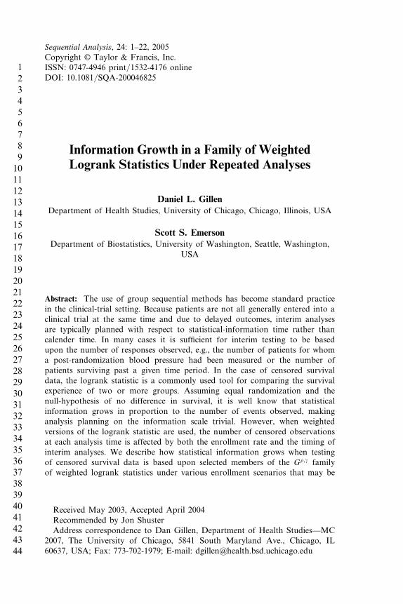
Sequential Analysis, 24: 1–22, 2005Copyright © Taylor & Francis, Inc.ISSN: 0747-4946 print/1532-4176 onlineDOI: 10.1081/SQA-200046825

Information Growth in a Family of WeightedLogrank Statistics Under Repeated Analyses

Daniel L. GillenDepartment of Health Studies, University of Chicago, Chicago, Illinois, USA

Scott S. EmersonDepartment of Biostatistics, University of Washington, Seattle, Washington,

USA

Abstract: The use of group sequential methods has become standard practicein the clinical-trial setting. Because patients are not all generally entered into aclinical trial at the same time and due to delayed outcomes, interim analysesare typically planned with respect to statistical-information time rather thancalender time. In many cases it is sufficient for interim testing to be basedupon the number of responses observed, e.g., the number of patients for whoma post-randomization blood pressure had been measured or the number ofpatients surviving past a given time period. In the case of censored survivaldata, the logrank statistic is a commonly used tool for comparing the survivalexperience of two or more groups. Assuming equal randomization and thenull-hypothesis of no difference in survival, it is well know that statisticalinformation grows in proportion to the number of events observed, makinganalysis planning on the information scale trivial. However, when weightedversions of the logrank statistic are used, the number of censored observationsat each analysis time is affected by both the enrollment rate and the timing ofinterim analyses. We describe how statistical information grows when testingof censored survival data is based upon selected members of the G�� familyof weighted logrank statistics under various enrollment scenarios that may be

Received May 2003, Accepted April 2004Recommended by Jon ShusterAddress correspondence to Dan Gillen, Department of Health Studies—MC

2007, The University of Chicago, 5841 South Maryland Ave., Chicago, IL60637, USA; Fax: 773-702-1979; E-mail: [email protected]

1234567891011121314151617181920212223242526272829303132333435363738394041424344

2 Gillen and Emerson

encountered in the clinical-trial setting. In addition, we consider the impacton estimation of treatment effects when performing an interim analysis at lessthan maximal information in the setting of nonproportional hazards survivaldata. A reweighting of the G�� statistic is proposed that reapportions unusedweight at interim analyses to a subset of the last observed events, therebyproviding estimates of treatment effect obtained at interim analyses that aremore comparable to those that would have been obtained had estimation beenperformed under full support.

Keywords: Censored data; Clinical trials; Information; Non-parametricstatistics; Sequential tests.

Mathematics Subject Classification: Primary 62L05; Secondary 62N.

1. INTRODUCTION

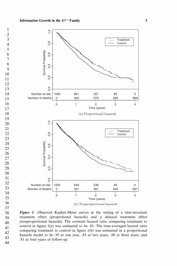
Time to a specified event such as death, myocardial infarction, or strokerepresents the primary outcome of interest in many clinical trials. Acommon strategy in this setting, and one we adopt here, is to basestatistical inference on the hazards of response, parameterizing treatmenteffects in terms of the hazard ratio �1�t�/�0�t�, where �i�t� represents theinstantaneous rate of failure in group i at time t given survival up to timet, i = 0� 1. When treatment effects are hypothesized to remain constantover time, such as simulated in figure 1(a), the logrank score statistic [8]is typically used to compare survival across treatment groups because itis known to be nearly fully efficient in this setting. However, treatmenteffects often vary with time, resulting in nonproportional hazards asdepicted with simulated data in figure 1(b). In order to gain efficiencyin such time-varying treatment-effect settings, various weighted versionsof the logrank statistic have been proposed. In particular, Fleming andHarrington [5] considered a general class of weighted logrank statisticstermed the G�� family, which encompasses both the usual logrankstatistic as well as the generalized Wilcoxon statistic [11].

Typically these weighted logrank statistics have been introducedand evaluated in the fixed sample setting. However, due to ethical andeconomic considerations, the use of group sequential methods has becomecommon in clinical trials. In order to maintain statistical and scientificintegrity, it is of utmost importance to fully evaluate the operatingcharacteristics of potential stopping rules at the design stage (see, forexample, Emerson et al. [12]). In general, a group sequential stopping rulefor the score statistic �j ∼N��Vj� Vj� is specified by a continuation setCj , for j = 1� � � � � J where j denotes the jth analysis of J total analyses.Under an independent increments structure, for a particular value of �

1234567891011121314151617181920212223242526272829303132333435363738394041424344

Information Growth in the G�� Family 3

Time (years)

Sur

viva

l Pro

babi

lity

0 1 2 3 4

0.0

0.2

0.4

0.6

0.8

1.0

TreatmentControl

Number at risk:Number of deaths:

10000

661340

257579

85656

0669

(a) Proportional hazards

Time (years)

Sur

viva

l Pro

babi

lity

0 1 2 3 4

0.0

0.2

0.4

0.6

0.8

1.0

TreatmentControl

Number at risk:Number of deaths:

10000

649351

239581

84645

0661

(b) Nonproportional hazards

Figure 1. Observed Kaplan-Meier curves in the setting of a time-invarianttreatment effect (proportional hazards) and a delayed treatment effect(nonproportional hazards). The constant hazard ratio comparing treatment tocontrol in figure 1(a) was estimated to be .85. The time-averaged hazard ratiocomparing treatment to control in figure 1(b) was estimated in a proportionalhazards model to be .95 at one year, .83 at two years, .80 at three years, and.81 at four years of follow-up.

1234567891011121314151617181920212223242526272829303132333435363738394041424344


the sampling density p�m��m �� for the test statistic �m��m�, m =1� � � � � J , �m ∈ �−�� is given by [2]

p�m�Um �m� ={f�m��m �� m � �m

0 otherwise(1)

where the function f�j��j �� is recursively defined as

f�1��1 �� =1√V1

(�1 − �V1√

V1

)f�j��j �� =

∫Cj−1

1√vj

(�j − u− �vj√

vj

)f�j − 1� u ��du� j = 2� � � � � m

with vj = Vj − Vj−1 for j = 2� � � � � m, and �x� = e−x2/2/√2� the density

of the standard normal distribution. In most situations vj will dependupon both the number of observed events accrued between analysis j − 1and j, as well as the variability of those observations.

Under a time-invariant treatment effect, (1) can be used to computethe operating characteristics of a given stopping rule. However, incomputing these operating characteristics, the value of vj given abovemust be defined, implying that a schedule of analyses defined accordingto the information fraction must be assumed. Further, in order tomaintain all operating characteristics computed during the design stage,adherence to the prespecified analysis times is required. Methods forflexible implementation of group sequential designs allowing for randomanalysis times and maintainance of some (but not all) operatingcharacteristics have been proposed for the independent incrementssetting [3, 6]. However, these methods still require some estimate ofinformation accrual in order to be properly implemented.

Tsiatis [1] demonstrated that a one-parameter subset of the G��

family achieved asymptotic independent increments, and thus how theabove approach for defining and implementing a sequential trial canbe used in this setting. Although the independent increments structureallows for easy computation of the density of these statistics undersequential testing, the estimation of information growth and treatmenteffects can be difficult when applying these statistics in a group sequentialsetting. Several authors have noted that in the case of the logrankstatistic, information growth is proportional to the number of eventsobserved when data exhibit proportional hazards and small departuresfrom the null hypothesis of equality of survival distributions [5, 10].In this situation, the planning of interim analyses is a straightforwardtask. However, this simple relationship between statistical informationaccrual and the number of observed events is not guaranteed to exist

1234567891011121314151617181920212223242526272829303132333435363738394041424344


when a weighted form of the logrank statistic is used [7] or undernonproportional hazards. Specifically, by applying a weighted logrankstatistic, one has implied that events occurring at one point in timeare more or less important (both clinically and statistically) thanevents occurring at some other point in time; thus the proportion ofinformation contributed by one event is not equal to that of anotheroccurring at a different event time.

In addition to information accrual, when using a weighted logrankstatistic one must also consider the estimation of treatment effects atinterim analyses. Keeping in mind that the only reason to choose aweighted version of the logrank statistic is due to the belief that hazardratios are likely to vary with time in some fashion, one must alsoconsider the impact of estimation of treatment effects when analyses areperformed at less than maximal information. For example, consider theKaplan-Meier curves in figure 1(b), which indicate a delayed treatmenteffect. In this setting the estimate of treatment effect calculated in aproportional hazards model at an interim analysis (occurring at less thanfour years) will be consistent for an effect that is smaller than that whichwould be estimated at an analysis occurring at four years. Because afixed sample test usually serves as a reference design when evaluatinggroup sequential stopping rules, the existence of time-varying treatmenteffects such as those portrayed in figure 1(b) can produce difficulties incomparing results obtained at an interim analysis to those that wouldhave been obtained under a single fixed sample test occurring at maximalinformation.

In the current manuscript, we will describe issues related to the useof weighted logrank statistics in clinical trials. In particular, we focuson the measurement of information growth with respect to the numberof observed events and consider the impact on estimation of treatmenteffects when performing an interim analysis based on a weighted logrankstatistic in the setting of nonproportional hazards-survival data. In section2 we describe the G�� family of weighted logrank statistics and defineproportionate information when these statistics are used during the courseof a trial. Section 3 considers information growth under staggered patientaccrual patterns. In section 4 we consider the estimation of treatmenteffects when analyses are performed at less than maximal information.We illustrate how the weighting scheme of the G�� statistic changes whensupport of the survival distribution is truncated due to an interim analysis.We also propose a reallocation of the weights employed by theG�� familyin an attempt to provide estimates of treatment effect that consistentlyestimate the same parameter at all interim analyses. Finally, in section 5we conclude with a discussion of the issues involved in performing interimanalyses where treatment effects are hypothesized to vary with time.

1234567891011121314151617181920212223242526272829303132333435363738394041424344


We consider other weighted statistics that could be used to comparesurvival in the clinical trial setting.

2. MEASURING RELATIVE INFORMATION IN THE G ��

FAMILY

Let Tik, Eik, and Cik denote the survival, entry, and censoring time ofindividual i, i = 1� � � � � mk, belonging to group k, k = 0� 1, where Tik, Eik,and Cik are assumed to be independent. Further, at analysis time � defineXik = min�Tik� �− Eik� Cik� to be the observed time for individual i ingroup k, and let ik = I�Xik = Tik� denote the indicator that the actualsurvival time is observed on the ith individual in group k. Finally, let

Nk�t� =mk∑i

I�Xik ≤ t� ik = 1�

denote the number of events observed in group k occurring prior to timet, and

Yk�t� =mk∑i

I�Xik ≥ t�

denote the number of patients at risk in group k at time t. The G��

statistic as defined by Fleming and Harrington [5] is given by

G�� =(M1 +M0

M1M0

)1/2 ∫ �

0w�t�

{Y1�t�Y0�t�

Y1�t�+ Y0�t�

}{dN1�t�

Y1�t�− dN0�t�

Y0�t�

}� (2)

and a consistent estimate of the variance of (2) can be computed as

�2 =(M1 +M0

M1M0

) ∫ �

0w2�t�

{Y1�t�Y0�t�

Y1�t�+ Y0�t�

}2{1− dN1�t�+ dN0�t�− 1

Y1�t�+ Y0�t�− 1

}×{d�N1�t�+ N0�t��

Y1�t�+ Y0�t�

}� (3)

where Mi denotes the number of patients initially at risk in group i, i =0� 1, and w�t� = �S�t−��1− S�t−��, with S�t−� denoting the Kaplan-Meier estimate of the pooled survival distribution of groups 0 and 1 justprior to time t. Fleming and Harrington [5] point out that because thequantity dNi�t�/Yi�t� in (2) consistently estimates the hazard for group iat time t, the G�� statistic can be viewed simply as a sum, over all failuretimes, of the weighted differences in the estimated hazards.

As noted in section 1, motivation for the use of such weightedlogrank statistics comes from the potential gain in efficiency that canbe obtained in the presence of nonproportional hazards. For instance,

1234567891011121314151617181920212223242526272829303132333435363738394041424344


taking � = 1 and � = 0 in the G�� family yields the generalized Wilcoxonstatistic [11], which applies increased weight to early failure times andresults in a more efficient statistic when early differences in survivalexist but wane over time. Another weighting pattern, obtained by taking� = � = 1, induces a quadratic weighting scheme, placing maximumweight on failures occurring at the time of pooled median survival,and less weight on failures occurring before and after. Note that for ahypothesized alternative such as the delayed treatment effect portrayedin figure 1(b), the weighting scheme defined by taking � = � = 1 wouldresult in increased efficiency when compared to the usual logrankstatistic, as it is placing greater relative weight on observations where thedifferences in hazards are largest.

In the clinical trial setting patients are likely to enter the trial in astaggered fashion, and loss-to-follow-up censoring and/or administrativecensoring, due to the freezing of a data set for analysis, is likely to occur.Following Tsiatis [1] and Lan et al. [7], under the null hypothesis H0 �

S0 = S1, the variance of the G�� statistic calculated at calendar time �

reduces to

�2 ∝∫ �

0w2�t�FE��− t��1− FC�t��dS�t�� (4)

where FE and FC denote the cumulative distribution function for theentry and censoring times, respectively.

Now consider repeated applications of the G�� statistic at interimanalysis times j = 1� � � � � J . Due to staggered entry, the number ofpatients initially at risk in each comparison group, Mi� i = 0� 1 will bedependent upon the analysis time. Hence we let Mi�j denote the numberof patients initially at risk in group i at analysis j. Further, let �2

j equalthe estimated variance of the G�� statistic applied at interim analysis j.Noting that the logrank test is a score test, obtained by differentiatingthe Cox partial likelihood and evaluating at the null hypothesis, we havethat the information for this statistic (and its weighted counterparts) isequal to the variance, and hence we define the proportion of informationat analysis j, relative to the maximal analysis J , as

�j ≡(M1�j +M0�j

M1�jM0�j

)−1

�2j

/(M1�J +M0�J

M1�JM0�J

)−1

�2J � (5)

where the normalizing constant has been removed from both thenumerator and denominator due to the potentially changing numbers ofpatients initially at risk at each analysis time.

1234567891011121314151617181920212223242526272829303132333435363738394041424344


3. INFORMATION GROWTH UNDER STAGGERED ACCRUALPATTERNS

Over the course of a clinical trial it is common for patients to haverandom entry times into the study. For example, in a study investigatinga new experimental treatment for lung cancer whose primary outcomeis death, not all patients are likely to be available to enter the study,but instead patients will be recruited over long periods of time. Undergroup sequential testing, interim analyses may be performed during therecruitment phase, because events are beginning to be observed for thosepatients entered into the study at earlier time points. From (4) above, itis clear that the distribution of patient entry times affects the variance ofthe G�� statistic, and hence the rate of information growth in this family.In this section we will consider the impact of changing patient-accrualpatterns upon the information growth for the G1�1 statistic.

3.1. Description of Accrual Patterns

Accrual patterns considered here were chosen to reflect those entry timesthat might be encountered during the course of a clinical trial. Often,the patient-accrual rate may change over time. For example, if one isconsidering the efficacy of a new experimental treatment for a diseasethat affects small numbers of individuals, it could be that at the startof the study a large number of patients will be recruited, though afterthese prevalent patients have been enrolled, accrual will begin to slowover time while investigators wait for incident patients to come to theirattention. On the other hand, it could be that as a trial continues on forlonger periods of time, additional centers will be recruited or cliniciansmay become more experienced recruiting their patients to enter the trial.In this setting, enrollment will increase with time. To address the issueof information growth when accrual patterns are nonuniform over time,we consider the situation where entry times, Eik, are chosen such that

Pr�Eik < t� =(t

�

)r

� with � > 0� r > 0� 0 < t ≤ �� (6)

Thus � controls the length of time over which patients could enter thetrial, while values of r close to 0 lead to right-skewed entry times andlarge values of r lead to left-skewed entry times. Note that taking r = 1in (7) results in entry times being distributed Unif�0� ��. In trials wheresolid recruiting procedures are in place at the inception of the study, auniform accrual pattern is quite plausible, allowing for a steady streamof patients to enter the study over time.

1234567891011121314151617181920212223242526272829303132333435363738394041424344


3.2. Uniform Entry

Under the null hypothesis H0 � S0 = S1, in the noncensored case, (4)reduces to a variance of the G�� statistic at analysis time � given by

�2 ∝∫ �

0w2�t�FE��− t�dS�t�� (7)

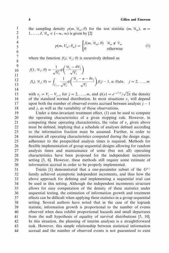
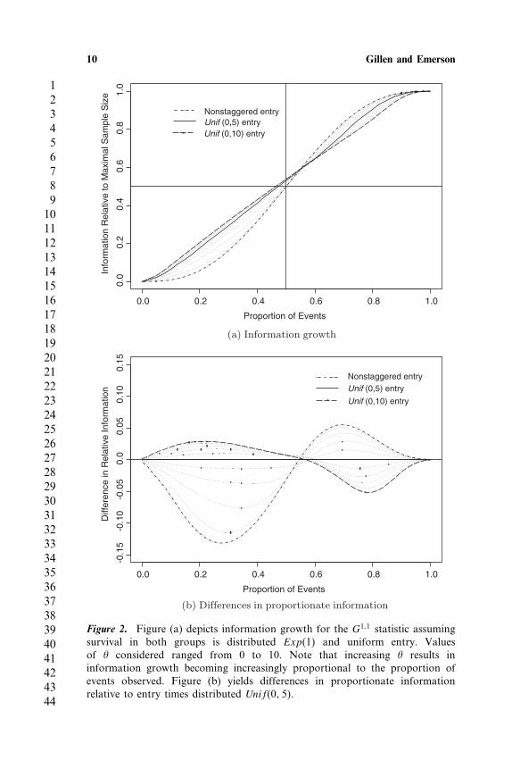
Figure 2 depicts information growth under the G1�1 statistic in thissetting as a function of the number of events observed for entry timesdistributed uniformly between 0 and �, � = 0� 2� 4� 6� 8� 10, with survivalin both groups distributed Exp�1�. When � is taken to be 0, implyingnonstaggered entry, the information growth curve is S-shaped, withmaximal information growth occurring at 50% survival. As � increases,the growth of information under the G1�1 statistic becomes increasinglyproportional to the number of events observed. Intuitively this isreasonable, for as � → � this would imply that at each event time, anew patient would enter the risk set, keeping the weight apportioned toeach observation relatively equal, though the constant of proportionalitydiffers from that of the unweighted logrank statistic.

3.3. Non-uniform Entry

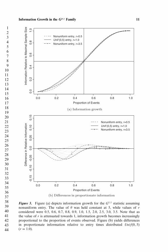
Figure 3 yields information growth under the G1�1 statistic when thecumulative distribution of entry times is assumed to equal the CDF givenin (7). For the purposes of illustration, � in (7) was held constant at 5while r was allowed to vary. Thus, taking r = 1 resulted in entry timesbeing distributed uniformly over the interval �0� 5�. Again, survival inboth groups was distributed Exp�1�. As the value of r is attenuatedtowards 1, the growth of information under the G1�1 statistic becomesincreasingly proportional to the number of events observed. This resultis in agreement with what was observed in the uniform entry case above,recognizing that as the value of r moves farther away from 1, thedistribution of entry times becomes more highly skewed, resembling anonstaggered-entry setting.

3.4. Incorrectly Assumed Entry Distributions

From (4) and sections 3.2 and 3.3, it is clear that the distribution ofentry times will affect the rate of information growth as well as themaximal information obtained when weighted logrank statistics are used.In practice one must assume some entry-time distribution when planning

1234567891011121314151617181920212223242526272829303132333435363738394041424344


Proportion of Events

Info

rmat

ion

Rel

ativ

e to

Max

imal

Sam

ple

Siz

e

0.0 0.2 0.4 0.6 0.8 1.0

0.0

0.2

0.4

0.6

0.8

1.0

Nonstaggered entryUnif (0,5) entryUnif (0,10) entry

(a) Information growth


Diff

eren

ce in

Rel

ativ

e In

form

atio

n

0.0 0.2 0.4 0.6 0.8 1.0

-0.1

5-0

.10

-0.0

50.

00.

050.

100.

15

Nonstaggered entryUnif (0,5) entry

Unif (0,10) entry

(b) Differences in proportionate information

Figure 2. Figure (a) depicts information growth for the G1�1 statistic assumingsurvival in both groups is distributed Exp�1� and uniform entry. Valuesof � considered ranged from 0 to 10. Note that increasing � results ininformation growth becoming increasingly proportional to the proportion ofevents observed. Figure (b) yields differences in proportionate informationrelative to entry times distributed Unif�0� 5�.

1234567891011121314151617181920212223242526272829303132333435363738394041424344



Info

rmat

ion

Rel

ativ

e to

Max

imal

Sam

ple

Siz

e

0.0 0.2 0.4 0.6 0.8 1.0

0.0

0.2

0.4

0.6

0.8

1.0

Nonuniform entry, r=0.5Unif (0,5) entry, r=1.0Nonuniform entry, r=3.5

(a) Information growth


Diff

eren

ce in

Rel

ativ

e In

form

atio

n

0.0 0.2 0.4 0.6 0.8 1.0

-0.1

5-0

.10

-0.0

50.

00.

050.

100.

15

Nonuniform entry, r=0.5Unif (0,5) entry, r=1.0Nonuniform entry, r=3.5

(b) Differences in proportionate information

Figure 3. Figure (a) depicts information growth for the G1�1 statistic assumingnonuniform entry. The value of � was held constant at 5, while values of rconsidered were 0.5, 0.6, 0.7, 0.8, 0.9, 1.0, 1.5, 2.0, 2.5, 3.0, 3.5. Note that asthe value of r is attenuated towards 1, information growth becomes increasinglyproportional to the proportion of events observed. Figure (b) yields differencesin proportionate information relative to entry times distributed Unif�0� 5�(r = 1�0).

1234567891011121314151617181920212223242526272829303132333435363738394041424344


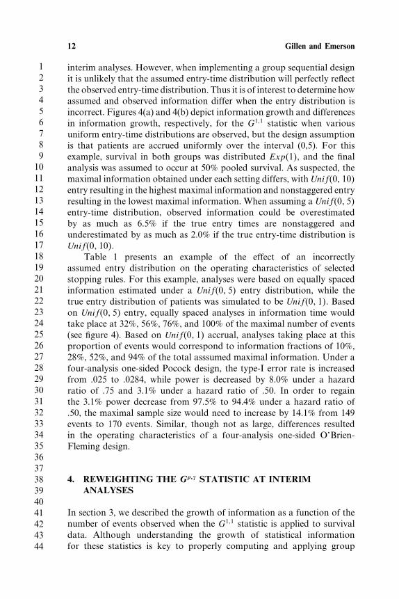
interim analyses. However, when implementing a group sequential designit is unlikely that the assumed entry-time distribution will perfectly reflectthe observed entry-time distribution. Thus it is of interest to determine howassumed and observed information differ when the entry distribution isincorrect. Figures 4(a) and 4(b) depict information growth and differencesin information growth, respectively, for the G1�1 statistic when variousuniform entry-time distributions are observed, but the design assumptionis that patients are accrued uniformly over the interval (0,5). For thisexample, survival in both groups was distributed Exp�1�, and the finalanalysis was assumed to occur at 50% pooled survival. As suspected, themaximal information obtained under each setting differs, with Unif�0� 10�entry resulting in the highest maximal information and nonstaggered entryresulting in the lowest maximal information. When assuming a Unif�0� 5�entry-time distribution, observed information could be overestimatedby as much as 6.5% if the true entry times are nonstaggered andunderestimated by as much as 2.0% if the true entry-time distribution isUnif�0� 10�.

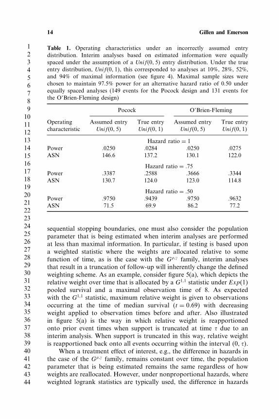
Table 1 presents an example of the effect of an incorrectlyassumed entry distribution on the operating characteristics of selectedstopping rules. For this example, analyses were based on equally spacedinformation estimated under a Unif�0� 5� entry distribution, while thetrue entry distribution of patients was simulated to be Unif�0� 1�. Basedon Unif�0� 5� entry, equally spaced analyses in information time wouldtake place at 32%, 56%, 76%, and 100% of the maximal number of events(see figure 4). Based on Unif�0� 1� accrual, analyses taking place at thisproportion of events would correspond to information fractions of 10%,28%, 52%, and 94% of the total asssumed maximal information. Under afour-analysis one-sided Pocock design, the type-I error rate is increasedfrom .025 to .0284, while power is decreased by 8.0% under a hazardratio of .75 and 3.1% under a hazard ratio of .50. In order to regainthe 3.1% power decrease from 97.5% to 94.4% under a hazard ratio of.50, the maximal sample size would need to increase by 14.1% from 149events to 170 events. Similar, though not as large, differences resultedin the operating characteristics of a four-analysis one-sided O’Brien-Fleming design.

4. REWEIGHTING THE G �� STATISTIC AT INTERIMANALYSES

In section 3, we described the growth of information as a function of thenumber of events observed when the G1�1 statistic is applied to survivaldata. Although understanding the growth of statistical informationfor these statistics is key to properly computing and applying group

1234567891011121314151617181920212223242526272829303132333435363738394041424344



Info

rmat

ion

Rel

ativ

e to

Max

imal

Sam

ple

Siz

e

0.0 0.2 0.4 0.6 0.8 1.0

0.0

0.2

0.4

0.6

0.8

1.0

Nonstaggered entryUnif (0,5) entry (assumed)Unif (0,10) entry

(a)


Ass

umed

Info

rmat

ion

- T

rue

Info

rmat

ion

0.0 0.2 0.4 0.6 0.8 1.0

-0.1

5-0

.10

-0.0

50.

00.

050.

100.

15

Nonstaggered entryUnif (0,5) entry (assumed)Unif (0,10) entry

(b)

Figure 4. Information growth (a) and differences in information growth (b)of the G1�1 statistic when Unif�0� �� entry-time distributions are observed, butthe design assumed a Unif�0� 5� entry-time distribution. Values of � consideredranged from 0 to 10. Survival in both groups was distributed Exp�1�, and thefinal analysis was assumed to occur at 50%.

1234567891011121314151617181920212223242526272829303132333435363738394041424344


Table 1. Operating characteristics under an incorrectly assumed entrydistribution. Interim analyses based on estimated information were equallyspaced under the assumption of a Unif�0� 5� entry distribution. Under the trueentry distribution, Unif�0� 1�, this corresponded to analyses at 10%, 28%, 52%,and 94% of maximal information (see figure 4). Maximal sample sizes werechosen to maintain 97.5% power for an alternative hazard ratio of 0.50 underequally spaced analyses (149 events for the Pocock design and 131 events forthe O’Brien-Fleming design)

Pocock O’Brien-Fleming

Operating Assumed entry True entry Assumed entry True entrycharacteristic Unif�0� 5� Unif�0� 1� Unif�0� 5� Unif�0� 1�

Hazard ratio = 1Power .0250 .0284 .0250 .0275ASN 146.6 137.2 130.1 122.0

Hazard ratio = �75Power .3387 .2588 .3666 .3344ASN 130.7 124.0 123.0 114.8

Hazard ratio = �50Power .9750 .9439 .9750 .9632ASN 71.5 69.9 86.2 77.2

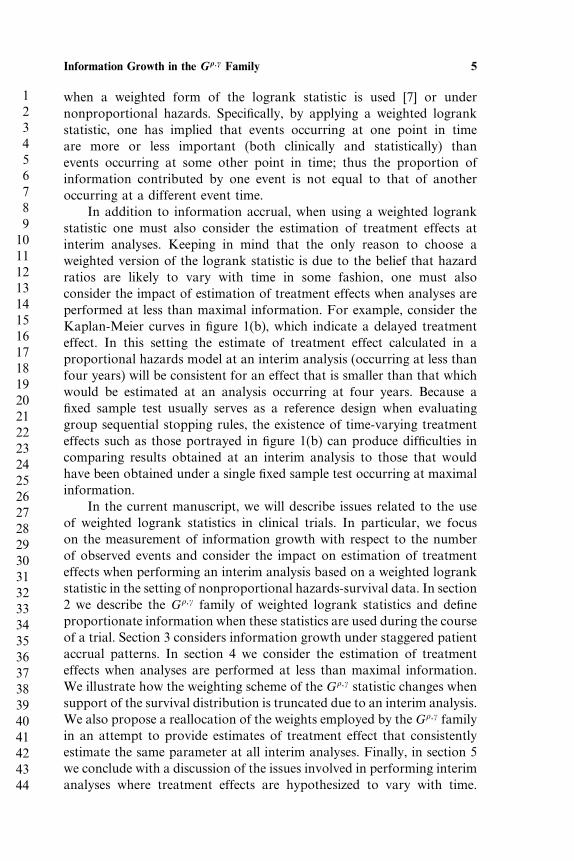
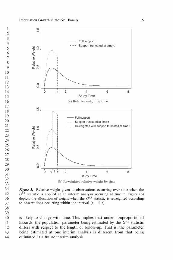
sequential stopping boundaries, one must also consider the populationparameter that is being estimated when interim analyses are performedat less than maximal information. In particular, if testing is based upona weighted statistic where the weights are allocated relative to somefunction of time, as is the case with the G�� family, interim analysesthat result in a truncation of follow-up will inherently change the definedweighting scheme. As an example, consider figure 5(a), which depicts therelative weight over time that is allocated by a G1�1 statistic under Exp�1�pooled survival and a maximal observation time of 8. As expectedwith the G1�1 statistic, maximum relative weight is given to observationsoccurring at the time of median survival (t = 0�69) with decreasingweight applied to observation times before and after. Also illustratedin figure 5(a) is the way in which relative weight is reapportionedonto prior event times when support is truncated at time � due to aninterim analysis. When support is truncated in this way, relative weightis reapportioned back onto all events occurring within the interval �0� ��.

When a treatment effect of interest, e.g., the difference in hazards inthe case of the G�� family, remains constant over time, the populationparameter that is being estimated remains the same regardless of howweights are reallocated. However, under nonproportional hazards, whereweighted logrank statistics are typically used, the difference in hazards

1234567891011121314151617181920212223242526272829303132333435363738394041424344


Study Time

Rel

ativ

e W

eigh

t

0 2 4 6 8

0.0

0.5

1.0

1.5

Full supportSupport truncated at time τ

τ

(a) Relative weight by time

Study Time

Rel

ativ

e W

eigh

t

0 2 4 6 8

0.0

0.5

1.0

1.5

Full supportSupport truncated at time τReweighted with support truncated at time τ

ττ−δ

(b) Reweighted relative weight by time

Figure 5. Relative weight given to observations occurring over time when theG1�1 statistic is applied at an interim analysis occuring at time �. Figure (b)depicts the allocation of weight when the G1�1 statistic is reweighted accordingto observations occurring within the interval ��− � ��.

is likely to change with time. This implies that under nonproportionalhazards, the population parameter being estimated by the G�� statisticdiffers with respect to the length of follow-up. That is, the parameterbeing estimated at one interim analysis is different from that beingestimated at a future interim analysis.

1234567891011121314151617181920212223242526272829303132333435363738394041424344


From a scientific perspective, the way in which weights are allocatedto a statistic over time should be determined by the clinical importanceof potential treatment effects that may be present at those times. Bydefining weights in such a way, one implicitly defines a populationparameter of interest, and hypotheses should be stated in terms of thisparameter. For example, we may consider testing the null hypothesisthat the sum of weighted differences in hazards over four years isequal to zero. Test statistics computed from observed data should thenconsistently estimate this parameter, providing evidence for or againstthe hypotheses of interest. By defining a weighting scheme via the useof a G�� statistic, one has defined a population parameter of interestrelative to some interval of time. However, by allowing the relativeweighting scheme to change due to the truncation of support inherentin interim testing, the population parameter being estimated by the G��

statistic also changes. This implies that a different hypothesis is beingtested at each analysis.

Clearly, it is not possible to accurately estimate a populationparameter that is defined over a fixed interval of time, say �0� T�, whendata have only been sampled up to time � < T . With this said, it maystill be possible to reallocate weights over the interval �0� �� in sucha way that data near time �, which may be highly correlated withunobserved data in the interval �� T�, are highly weighted. Thus, thegoal is to take advantage of potential time trends in the data in order toattempt to consistently estimate the same parameter of interest from oneinterim analysis to the next. Formally, one might consider a modifiedG�� weighting scheme of the form

w∗�t� =

w�t�

( ∫ �0 w�x�dx∫ T0 w�x�dx

)if t <

w�t�( ∫ �

0 w�x�dx∫ T0 w�x�dx

)+ −1

∫ �

0 w�x�dx[1−

∫ �0 w�x�dx∫ T0 w�x�dx

]if t ≥

(8)

where w�t� = S�t−��1− S�t−�� and ∈ �0� �� is chosen a priori anddictates the interval of time over which weights are to be reallocated.Figure 5(b) illustrates the effect of the reweighting scheme given in(8). By reweighting at time �, the relative weight prescribed to thoseobservations occurring in the interval �0� �− � remains the same asit would have been had the full support of the survival distributionbeen sampled, with the unused mass being reapportioned to observationsoccurring within the interval ��− � ��. In practice, one could choose simply based upon a meaningful time interval, although in order toensure an adequate number of events to be reweighted, it may be morereasonable to choose a percentage of the total number of events, such asthe last 10–50% of observed events, to reweight.

1234567891011121314151617181920212223242526272829303132333435363738394041424344


The motivation for using a reweighting scheme as defined in (8)attempts to modify the G�� statistic so that the same parameter ofinterest is being consistently estimated at each interim analysis. Note thatthis differs from the concept of stochastic curtailment, which attemptsto estimate the value of the test statistic that would be observed at thefinal analysis. With this said, reapportioning the weights in such a waythat attempts to take advantage of late-occurring trends in the data couldcertainly provide insight into the value of test statistics that might beobserved at the final analysis.

By emphasizing late-occurring trends in the data, the reweightedstatistic defined above may be more powerful than a non-reweightedstatistic when hazards diverge late, as depicted by the survival curvesin figure 1(b). However, the variance of the statistic will also increase,sometimes substantially, when interim analyses are performed, because alarge portion of weight is being reallocated to a relatively few numberof observations (depending on the choice of ). Intuitively, this behaviorshould seem reasonable when considered in light of the weighting schemechosen with full support in mind. That is, when information accrualis low, implying that a large portion of weight remains unused, thevariability in our statistic should reflect this. For example, consider thedelayed treatment-effect data displayed in figure 1(b), where one mightreasonably consider a weighting scheme such as that defined by theG1�1 statistic. When considering this type of delayed effect, any multiple-testing procedure should behave conservatively at early analyses withrespect to decisions in favor of futility. Clearly, extremely conservativestopping boundaries can be utilized to address this, but by basing testsupon the reweighted statistic described above, early conservatism of theprocedure can inherently be built into the statistic, reducing the need togreatly modify standard stopping rules.

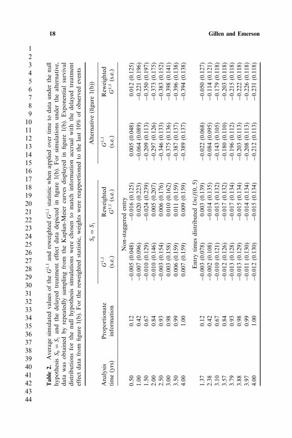
To illustrate the effect of reweighting the G�� statistic at differentinformation fractions, table 2 displays simulated values of the G1�1

and reweighted G1�1 statistic when applied to data simulated underthe null hypothesis S0 = S1 and data sampled from the Kaplan-Meiercurves given in figure 1(b). Exponential survival distributions for the nullhypothesis simulations were chosen to match information accrual withthe delayed treatment-effect data from figure 1(b). Similarly, analysistimes for the staggered enrollment case were chosen to match up with theproportionate information accrued at each analysis in the nonstaggeredcase. Mean values across 500 simulations are given for each parameterestimate. For purposes of illustration, weights were reapportioned to thelast 10% of observed events at each analysis. Under both nonstaggeredand Unif�0� 5� entry, when the null hypothesis is true, both the G1�1

statistic and the reweighted G1�1 statistic are consistently estimatinga null effect at all analysis times. In contrast, under the alternative

1234567891011121314151617181920212223242526272829303132333435363738394041424344


Tab

le2.

Average

simulated

values

oftheG

1�1an

dreweigh

tedG

1�1statisticwhenap

pliedov

ertimeto

data

underthenu

llhy

pothesis

S0=

S1an

dthedelayed

treatm

enteffect

data

depicted

infig

ure1(b).For

simulations

underthealternative,

data

was

obtained

byrepeatedly

samplingfrom

theKap

lan-Meier

curves

displayed

infig

ure1(b).Exp

onential

survival

distribu

tion

sforthenu

llhy

pothesis

simulations

werechosen

tomatch

inform

ation

accrua

lwith

thedelayed

treatm

ent

effect

data

from

figure1(b).For

thereweigh

tedstatistic,

weigh

tswerereap

portionedto

thelast

10%

ofob

served

events

S0=

S1

Alterna

tive

(figu

re1(b))

Ana

lysis

Propo

rtiona

teG

1�1

Rew

eigh

ted

G1�1

Rew

eigh

ted

time(yrs)

inform

ation

(s.e.)

G1�1(s.e.)

(s.e.)

G1�1(s.e.)

Non

-stagg

ered

entry

0.50

0.12

−0�005

(0.048

)−0

�016

(0.125

)0.00

5(0.048

)0.01

2(0.125

)1.00

0.42

−0�007

(0.096

)0.02

0(0.223

)−0

�064

(0.089

)−0

�221

(0.196

)1.50

0.67

−0�010

(0.129

)−0

�024

(0.239

)−0

�209

(0.113

)−0

�350

(0.197

)2.00

0.84

−0�010

(0.146

)0.00

5(0.207

)−0

�297

(0.126

)−0

�373

(0.175

)2.50

0.93

−0�003

(0.154

)0.00

6(0.176

)−0

�346

(0.133

)−0

�383

(0.152

)3.00

0.98

0.00

3(0.158

)0.01

0(0.162

)−0

�375

(0.136

)−0

�398

(0.141

)3.50

0.99

0.00

6(0.159

)0.01

1(0.159

)−0

�387

(0.137

)−0

�396

(0.138

)4.00

1.00

0.00

7(0.159

)0.00

9(0.159

)−0

�389

(0.137

)−0

�394

(0.138

)

Entry

times

distribu

tedUnif�0�5�

1.37

0.12

−0�003

(0.078

)0.00

3(0.139

)−0

�022

(0.068

)−0

�050

(0.127

)2.38

0.42

−0�002

(0.108

)−0

�014

(0.135

)−0

�084

(0.095

)−0

�114

(0.121

)3.10

0.67

−0�010

(0.121

)−0

�013

(0.132

)−0

�143

(0.105

)−0

�179

(0.118

)3.57

0.84

−0�012

(0.126

)−0

�017

(0.132

)−0

�180

(0.110

)−0

�203

(0.118

)3.79

0.93

−0�013

(0.128

)−0

�017

(0.134

)−0

�196

(0.112

)−0

�215

(0.118

)3.88

0.98

−0�013

(0.129

)−0

�015

(0.134

)−0

�203

(0.113

)−0

�222

(0.118

)3.97

0.99

−0�011

(0.130

)−0

�014

(0.134

)−0

�208

(0.113

)−0

�226

(0.118

)4.00

1.00

−0�012

(0.130

)−0

�015

(0.134

)−0

�212

(0.113

)−0

�231

(0.118

)

1234567891011121314151617181920212223242526272829303132333435363738394041424344


hypothesis assuming nonstaggered entry, we can see that with theexception of the first analysis occurring at six months where no treatmenteffect had yet been observed, the reweighted G1�1 statistic more closelyapproximates the value of the G1�1 statistic computed after samplinga full four years of support. For example, at eighteen months it wasestimated that 67% of the maximal trial information had been sampled,and the usual G1�1 statistic estimated a treatment effect less than half ofthat when using full support. In contrast, the reweighted G1�1 statisticcalculated at eighteen months closely approximates the value of theG1�1 statistic calculated at four years. Similar patterns were observedunder the alternative hypothesis assuming Unif�0� 5� entry. However,under staggered entry, analysis times were shifted later to maintainproportionate information. In this case a greater amount of the fullsupport was sampled at early analyses, and thus less reweighting wasneeded. It should also be noted that in each case, the G1�1 statistic and itsreweighted counterpart do not agree at the final analysis. This is becausefull support was assumed to be over the entire four years and, in general,the final event time in each simulation occurred at less than four years.Some reweighting of the G1�1 statistic occurred even at the four-yearanalysis.

In all four cases, it can be seen that the variability of thereweighted statistic is increased relative to the usual G1�1 statistic whenproportionate information is low, yielding a rather conservative testingprocedure at early analyses. When hypothesizing a delayed treatmenteffect, this conservatism can preclude one from stopping a trial tooearly with a decision in favor of futility without having viewed the fullsupport of the survival distribution—an important point if late-occurringpatterns in the data point to a beneficial treatment effect. For example,consider the twelve-month analysis (42% maximal information) underthe alternative hypothesis presented in table 2. Under nonstaggeredenrollment, the reweighted statistic estimates some beneficial treatmenteffect (point estimate of −0�221), while the usual G1�1 statistic results ina point estimate of only −0�064. In this case, without reweighting thestatistic one would be more likely to stop early in favor of futility withoutgoing on to witness the late-emerging treatment effects in the data. Onthe other hand, under the null hypothesis the reweighted statistic stillconsistently estimates a null effect at each analysis time, implying that ifno late-occurring evidence of a beneficial treatment effect is observed, adecision in favor of futility will ultimately be reached.

One drawback to the reweighted statistic is that it relies on a “lastone carried forward” procedure for estimating treatment effects, in thatit assumes that hazard differences occurring in the interval ��− � �� arethe same as those that would be observed in the interval � � T�. Clearlythis need not be the case, and it is possible to reweight observations in an

1234567891011121314151617181920212223242526272829303132333435363738394041424344


interval of time that are not representative of future results. The strategydemonstrated here is based on the presumption that later-occurringevents are more highly informative about future events. One may wishto choose even larger values of to avoid placing large mass on intervalsof time that may not be representative of unsampled support.

Another disadvantage to using the reweighted statistic lies in thecalculation of w∗�t�. As the definition of w∗�t� in (8) involves

∫ T

0 w�x�dx,it is necessary to estimate S�t� for � < t ≤ T . Extrapolation of thesurvival curve can be done by using a piecewise exponential (constanthazard) or Weibull (log-linear hazard) model to estimate the cumulativehazard, ��t�, for � < t ≤ T using observed event times prior to time �,then estimating S�t� as e−��t�. Although these methods for extrapolatingsurvival are parametric, they are only used to estimate the amountof weight that should be reallocated to the G�� statistic. Becausethe focus of the G�� statistic remains on comparing differences innonparametrically estimated hazards, this parametric extrapolation ofthe survival curves, which only affects the amount of weight to bereallocated, does not detract from the nonparametric nature of theweighted logrank statistic. Of course, this problem arises because theweights utilized by the G�� statistic are a function of the pooled survivalestimate of the comparison groups. If weights instead are chosen basedupon clinically relevant times alone, as suggested by Gillen and Emerson[4], the proportion of weight to be reallocated would be defined by thetiming of interim analyses and would not require estimation.

Finally, because the weighting scheme of the reweighted statistic ischanging at each interim analysis, it is easy to show that an independentincrements structure is no longer maintained. This implies that thesequential density in (1) can no longer be used to compute stoppingboundaries; however, straightforward simulation techniques can be usedto calculate stopping rules that control the overall level of the groupsequential test (see, for example, [13]).

5. DISCUSSION

In a clinical setting where treatment effects are hypothesized to vary withtime, weighted logrank statistics, such as those belonging to the G��

family, are sometimes used to compare survival across treatment groups.When evaluating the operating characteristics of group sequentialstopping rules, it is necessary to specify the timing of interim analyses,typically defined by the information fraction or the fraction of totalstatistical information available at the time of the interim analysis.Although methods for flexible implementation of group sequentialdesigns allowing for random analysis times have been proposed [3, 6],

1234567891011121314151617181920212223242526272829303132333435363738394041424344


these methods still require some estimate of information accrual inorder to be properly implemented. In the case of the logrank statistic,information grows proportionally to the number of observed events.However, when weighted logrank statistics are employed, informationgrowth can differ greatly from that of the usual logrank statistic.

We have presented a procedure for estimating information growthin the G�� family and demonstrated the dependence of informationgrowth within this family on the underlying censoring and patient entry-time distributions. In practice, when planning a clinical trial one mustobtain reasonable estimates of patient-accrual patterns and potentialcensoring that may be encountered. By adequately considering staggeredaccrual and censoring, it is possible to reasonably estimate informationgrowth and appropriately schedule analyses when these weighted logrankstatistics are used.

In addition to information accrual, one must also consider theestimation of treatment effects at interim analyses when using a weightedlogrank statistic. We have suggested a reweighting of the G�� statisticthat reapportions unused weight at interim analyses to a subset ofthe last observed events. By using such a reweighting scheme we havedemonstrated that estimates of treatment effect obtained when analysesare performed at less than maximal information are more comparableto those that would have been obtained had estimation been performedunder full support. It was also shown that the proposed reweightingprocedure builds in a degree of early conservatism by increasing thevariability of the G�� statistic when computed at times where theproportion of maximal information is low. Clearly, if one is expectingtreatment effects to vary with time, it seems reasonable to considertesting procedures that incorporate such early conservatism.

The reweighting procedure we have proposed is not unique to theG�� statistic, but can be used for any statistic employing a weightingscheme dependent upon time. In particular, Gillen and Emerson [4] haveshown that the G�� class of statistics demonstrates nontransitivity undernonproportional hazards and have proposed various weighting schemesfor the differences in hazards that do maintain transitivity at all times.In addition, Pepe and Fleming [9] proposed using a statistic based onthe sum of weighted differences in survival, and Murray and Tsiatis[13] consider this statistic under interim analyses, pointing out thatin many situations this statistic provides a more clinically meaningfulestimate of treatment effect than the G�� class that compares hazards.In both cases, a time-weighted estimate of treatment effect is considereddue to a hypothesized interaction between treatment and time, andthe reweighting procedure considered here would apply equally well insettings where interim analyses are performed.

1234567891011121314151617181920212223242526272829303132333435363738394041424344


ACKNOWLEDGMENTS

The authors would like to thank the associate editor and reviewer forinsightful comments and suggestions that considerably improved thismanuscript.

REFERENCES

1. Anastasios A. Tsiatis. (1982) Repeated significance testing for a generalclass of statistics used in censored survival analysis, Journal of the AmericanStatistical Association, 77: 855–861.

2. Armitage, P., McPherson, C. K., Rowe, B. C. (1969) Repeated significancetests on accumulating data, Journal of the Royal Statistical Society, Series A,General, 132: 235–244.

3. Bart E. Burington, Scott S. Emerson. (2003) Flexible implementations ofgroup sequential stopping rules using constrained boundaries, Biometrics,59: 770–777.

4. Daniel L. Gillen, Scott S. Emerson. (2003) Non-transitivity in a class ofweighted logrank statistics under non-proportional hazards, Submitted forpublication.

5. Fleming, T. R. and Harrington, D. P. (1991) Counting Processes andSurvival Analysis, Wiley.

6. Gordan Lan, K. K., David L. DeMets. (1983) Discrete sequentialboundaries for clinical trials, Biometrika, 70: 659–663.

7. Gordan Lan, K. K., William F. Rosenberger, John M. Lachin. (1995)Sequential monitoring of survival data with the Wilcoxon statistic,Biometrics, 51: 1175–1183.

8. Mantel, N. (1966) Evaluation of survival data and two new rank orderstastistics arising in its consideration, Cancer Chemo. Rep., 50: 163–170.

9. Margaret Sullivan Pepe, Thomas R. Fleming. (1989) Weighted Kaplan-meier statistics: A class of distance tests for censored survival data,Biometrics, 45: 497–507.

10. Mitchell H. Gail, David L. DeMets, Eric V. Slud. (1982) Simulationstudies on increments of the twosample logrank score test for survival timedata, with application to group sequential boundaries, in Survival Analysis,pp. 287–301. Institute of Mathematical Statistics (Hayward).

11. Prentice, R. L. (1978) Linear rank tests with right censored data (corr: V70p. 304), Biometrika, 65: 167–180.

12. Scott S. Emerson, John M. Kittelson, Daniel L. Gillen. (2003) Evaluatinggroup sequential designs, UW Biostatistics Working Paper Series. WorkingPaper 216. http://www.bepress.com/uwbiostat/paper 216.

13. Susan Murray, Anastasios A. Tsiatis. (1999) Sequential methods forcomparing years of life saved in the two-sample censored data problem,Biometrics, 55: 1085–1092.

Documents

Information Growth in a Family of Weighted Logrank Statistics Under