Information geometry and prior selectionomega.albany.edu:8008/ignorance/snoussi02.pdf · Information geometry and prior selection Hichem Snoussi and Ali Mohammad-Djafari Laboratoire

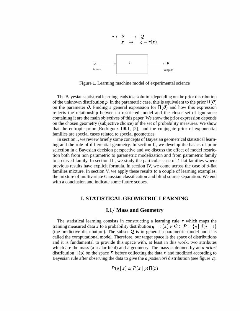
Information geometry and prior selection

Hichem Snoussi�

and Ali Mohammad-Djafari�

�Laboratoire des Signaux et Systèmes (L2S),

Supélec, Plateau de Moulon, 91192 Gif-sur-Yvette Cedex, France

Abstract. In this contribution, we study the problem of prior selection arising in Bayesian infer-ence. There is an extensive literature on the construction of non informative priors and the subjectseems far from a definite solution [1]. Here we revisit this subject with differential geometry toolsand propose to construct the prior in a Bayesian decision theoretic framework. We show how theconstruction of a prior by projection is the best way to take into account the restriction to a partic-ular family of parametric models. For instance, we apply this procedure to the curved parametricfamilies where the ignorance is directly expressed by the relative geometry of the restricted modelin the wider model containing it.

INTRODUCTION

Experimental science can be modeled as a learning machine mapping the inputs � tothe outputs � (see figure � ). The complexity of the physical mechanism underlying themapping inputs/outputs or the lack of information make the prediction of the outputsgiven the inputs (forward model) or the estimation of the inputs given the outputs (in-verse problem) a difficult task. When a parametric forward model �� is assumedto be available from the knowledge of the system, one can use the classical ML orwhen a prior model �� is assumed to be available too, the classicalBayesian methods can be used to obtain the joint a posteriori �� and then both�� and �� from which we can make any inference about � and . But in manypractical situations the question of modeling �� and �� is still open and to vali-date a model, one uses what is called the training data � � � �� ! " . Then the role ofstatistical learning become trying to find a joint distribution ��#� � belonging in general tothe whole set of probability distributions and to exploit the maximum of relevant infor-mation to provide some desired predictions. In this paper, we suppose that we are givensome training data �$�� ! " and � �� ! " and some information about the mapping which con-sists in a model % �'&)( �#� �+* of probability distributions, parametric ( % �,&)( �#�- ��+* )or non parametric. Our objective is to construct a learning rule . mapping the set / oftraining data � � � �$�� ! "�� ! "0� to a probability distribution �213% or to a probabilitydistribution in the whole set of probabilities �4165 :

.478/ 9�: %� ;: < � .=�#� �inputs outputs

> ?@Figure � . Learning machine model of experimental science

The Bayesian statistical learning leads to a solution depending on the prior distributionof the unknown distribution � . In the parametric case, this is equivalent to the prior AB� ��on the parameter . Finding a general expression for AB� �� and how this expressionreflects the relationship between a restricted model and the closer set of ignorancecontaining it are the main objectives of this paper. We show the prior expression dependson the chosen geometry (subjective choice) of the set of probability measures. We showthat the entropic prior [Rodriguez �DCECF� , [2]] and the conjugate prior of exponentialfamilies are special cases related to special geometries.

In section I, we review briefly some concepts of Bayesian geometrical statistical learn-ing and the role of differential geometry. In section II, we develop the basics of priorselection in a Bayesian decision perspective and we discuss the effect of model restric-tion both from non parametric to parametric modelization and from parametric familyto a curved family. In section III, we study the particular case of G -flat families whereprevious results have explicit formula. In section IV, we come across the case of G -flatfamilies mixture. In section V, we apply these results to a couple of learning examples,the mixture of multivariate Gaussian classification and blind source separation. We endwith a conclusion and indicate some future scopes.

I. STATISTICAL GEOMETRIC LEARNING

I.1 H Mass and Geometry

The statistical learning consists in constructing a learning rule . which maps thetraining measured data � to a probability distribution < � .�� 1I%KJL5 �M& �6ON�� *(the predictive distribution). The subset % is in general a parametric model and it iscalled the computational model. Therefore, our target space is the space of distributionsand it is fundamental to provide this space with, at least in this work, two attributeswhich are the mass (a scalar field) and a geometry. The mass is defined by an a prioridistribution A-�P� � on the space 5 before collecting the data � and modified according toBayesian rule after observing the data to give the a posteriori distribution (see figure Q ):( �P�R+� ��SM( �#�T�� A-�P� �

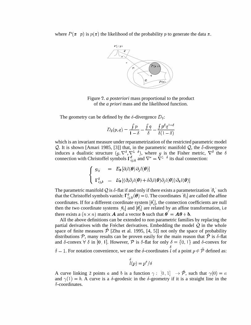
where ( ��T�� is �� the likelihood of the probability � to generate the data � .UEVXW�Y Z�[U\V Z]Y W#[

^_

UEV Z�[`..WRa bc

Figure Q . a posteriori mass proportional to the productof the a priori mass and the likelihood function.

The geometry can be defined by the G -divergence de :dfeD�P� � < �=� N��g9hGji Nk<G 9 N$� e < ��l eGm�n�o9hG �

which is an invariant measure under reparametrization of the restricted parametric model% . It is shown [Amari 1985, [3]] that, in the parametric manifold % , the G -divergenceinduces a dualistic structure ��p ��q e ��q ��l e � , where p is the Fisher metric, q e the Gconnection with Christoffel symbols r e�Xsnt u and q4vg�Kq ��l e its dual connection:wxXy p �!s � z�{}|X~E�� =��~)s�� r e�Xsnt u � z�{}| � ~E��~)s�� =� i G ~E�� ~�s�� ~\u�� The parametric manifold % is G -flat if and only if there exists a parameterization |��)�� suchthat the Christoffel symbols vanish: r e�Xs�t u � �� . The coordinates |��D�� are called the affinecoordinates. If for a different coordinate system |X�E�� , the connection coefficients are nullthen the two coordinate systems |X�� and |X�)�� are related by an affine transformation, i.ethere exists a �� matrix � and a vector � such that � � � i � .All the above definitions can be extended to non parametric families by replacing thepartial derivatives with the Fréchet derivatives. Embedding the model % in the wholespace of finite measures �5 [Zhu et al. 1995, [4, 5]] not only the space of probabilitydistributions 5 , many results can be proven easily for the main reason that �5 is G -flatand G -convex ��G in |X�� . However, 5 is G -flat for only G �8&)�m� � * and G -convex forG � � . For notation convenience, we use the G -coordinates

e � of a point �41��5 defined as:e � �P� �=� � e�� GA curve linking Q points � and � is a function ��7 |X�� 9�: �5 , such that �� \�� and �g�� . A curve is a G -geodesic in the G -geometry if it is a straight line in theG -coordinates.

I.2 H Bayesian learning

The loss quantity of a decision rule . with a fixed G -geometry can be measured bythe G -divergence dfeD�P� � .��#� � � between the true probability � and the decision .=�#� � . Thisdivergence is first averaged with respect to all possible measured data � and then withrespect to the unknown true probability � which gives the generalization error z ��. � :z eD��. ��K¡�¢�( �P� �E¡m£�( �#�-¤� � d�e¥�P� � .��#� � �Therefore, the optimal rule .De is the minimizer of the generalization error:.¦e �K§�¨ ©�ª«�¬ &)z e��. �+*The coherence of Bayesian learning is shown in [Zhu et al. 1995, [4, 5]] and means thatthe optimal estimator .¥e can be computed pointwise as a function of � and we don’t needa general expression of the optimal estimator .�e :®�� =� .¦e�� K§�¨�©�ª4«�¬¯ ¡ ¢�( �P�°�� d�e¥�P� � < � (1)

By variational calculation, the solution of (1) is straightforward and gives:®� e � ¡ � e ( �P�°�± �The above solution is exactly the gravity center of the set �5 with mass ( �P�°�� , the aposteriori distribution of � and the G -geometry induced by the G -divergence d6e . Here wehave the analogy with the static mechanics and the importance of the geometry definedon the space of distributions. The whole space of finite measures �5 is G -convex andthus, independently on the a posteriori distribution ( ��°�� the solution

®� belongs to �5�6G²1 |X�� .I.3 H Restricted Model

In practical situations, we restrict the space of decisions to a subset %³1´�5 . % is ingeneral a parametric manifold that we suppose to be a differentiable manifold. Thus % isparametrized with a coordinate system |��¶µ�P�� where � is the dimension of the manifold.% is also called the computational model and we prefer this appellation because the mainreason of the restriction is to design and manipulate the points � with their coordinateswhich belong to an open subset of · µ . However, the computational model % is notdisconnected from non parametric manipulations and we will show that both a prioriand final decisions can be located outside the model % .

Let’s compare now the non parametric learning with the parametric learning when weare constrained to a parametric model % :

1. Non parametric modeling: The optimal estimate is the minimizer of the gener-alization error where the true unknown point � is allowed to belong to the whole

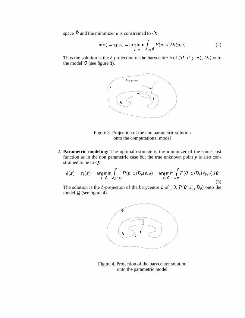
space �5 and the minimizer < is constrained to % :®<F�#� �� .¥eD�#� �=�¸§�¨ ©�ª4«�¬¯n¹Eº ¡�¢ ¹g»¼ ( ��°�� d�e¥�P� � < � (2)

Thus the solution is the G -projection of the barycentre®� of ��5 ��( �P�°�� d�e � onto

the model % (see figure ½ ).

º ¾ ¿¾¿À»¼ Á -projection

Figure ½ . Projection of the non parametric solutiononto the computational model

2. Parametric modeling: The optimal estimate is the minimizer of the same costfunction as in the non parametric case but the true unknown point � is also con-strained to be in % :®<O�� .¦e�� =�K§�¨�©�ª«�¬¯�¹�º ¡�¢ ¹Eº ( ��°�� d�e¥�P� � < �=�¸§�¨ ©�ª4«�¬¯�¹Eº ¡ { ( � �� d�e��P� @ � < ��Âo

(3)The solution is the G -projection of the barycentre

®� of �]% �D( � �� de � onto themodel % (see figure Ã ).

º»¼

¿¾Figure Ã . Projection of the barycentre solution

onto the parametric model

The interpretation of the parametric modeling as a non parametric one and the effectof such restriction can be done in two ways:

1. The cost function to be minimized in equation (3) is the same as the cost functionin (2) when � is allowed to belong to the whole set �5 and the a posteriori ( ��°�� iszero outside the model % . This is the case when the prior ( �� has % as its support.However this interpretation implies that the best solution

®� which is the barycentreof % can be located outside the model % and thus has a priori a zero probability !

2. The second interpretation is to say that the cost function to be minimized inequation (3) is the same as the cost function in (2) when the a posteriori ( � �� is the projected mass of the a posteriori ( �P�°�� onto the model % . We note herethe role of the geometry defined on the space 5 and the relative geometric shape ofthe manifold. For instance, the ignorance is directly related to the geometry of themodel % . The projected a posteriori or a priori can be computed by:Ä�Å ��< ��S ¡ ¢ ¹¦Æ ` Ä �P� �where

Ä �� designs the a priori or the a posteriori distribution and Ç ¯ �È& �I1�5É�� Å � < * the set of points � whose the G -projection is the < in % .The manipulation of these concepts in the general case is very abstract. However, insection IV, we present the explicit computations in the case of restricted autoparallelparametric submanifold % � 1�% of G -flat families.

II. PRIOR SELECTION

The present section is the main contribution of this paper. We address here the problemof prior selection in a Bayesian decision framework. By prior selection, we mean howto construct a prior ( �P� � respecting the following rule: Exploit the prior knowledgewithout adding irrelevant information. We note that this represents a trade off betweensome desirable behaviour and uniformity of the prior. We want to insist here, that theprior selection must be performed before collecting the data � , otherwise the coherenceof the Bayesian rule is broken down.

In a decision framework, the desirable behaviour can be stated as follows: Beforecollecting the training data, provide a reference distribution ��Ê as a decision. The refer-ence distribution can be provided by an expert or by our previous experience. Now, wehave the inverse problem of the statistical learning. Before, the a posteriori distribution(mass) is fixed and we have to find the optimal decision (barycentre). Now, the opti-mal decision �ËÊ (barycentre) is fixed and we have to find the optimal repartition AB�P� �according to the uniformity constraint. In order to have the usual notions of integrationand derivation, we assume that our objective is to find the prior on the parametric model% �Ì& < @ 1ÎÍÏJÐ· µ * .

The cost function can be constructed as a weighted sum of the generalization error ofthe reference prior and the divergence of the prior from the Jeffreys prior (The squareroot of the determinant of the Fisher information [6]) representing the uniformity. It is

worth noting that we are considering two different spaces: the space �5 of finite measuresand the space of prior distributions on the finite measures. Since we have two distinctspaces, we can choose two different geometries on each space. For example, if weconsider the G -geometry on the space �5 and the � -geometry on the space of priors,we have the following cost function:Ñ �#A �� ÓÒ ¡ AB� �� d�eD�P� @ � ��Ê �nÂg i �ÓÔ ¡ A-� ��Õ�ÖE© AB� =� �Ë× p�� nÂg (4)

where �mÒ is the confidence degree in the reference distribution ��Ê and �ØÔ the uniformitydegree. Considered independently, these two coefficients are not significant. However,their ratio is relevant in the following. The cost (4) can be rewritten as:wxXy Ñ ��A �� ÓÒ z ��.¥Ê � i �ØÔ�NÙAB� ��Õ�ÖE© AB� �� × p�� Âo Ú #ÛÚ £ �K�where z ��.¥Ê � is the generalisation error of a fixed learning rule .�Ê . By variational calcu-lation, we obtain the solution of the minimization of the function (4):A-� ��=SMÜ l�ÝßÞÝ#àÓá Á â ¢�ã t ¢ Û�ä × p�� (5)

We note that if G � � then the cost function (4) is the kullback-Leibler divergencebetween the joint distributions of data and parameters as considered in [Rodriguez 1991,[2]] and if G �¸� we obtain the conjugate prior for exponential families (see examples insection VI). When the value of the ratio �FÒ � �ØÔ goes to � , we obtain the Jeffreys prior andwhen this ratio goes to å we obtain the Dirac concentrated on ��Ê .

The model restriction to the parametric manifold % is essentially for computationalreasons. However, the reference distribution is a prior decision and does not depend on apost processing after collecting the data. Therefore, the reference distribution ��Ê can belocated in the whole space of probability measures. We can also have either a discrete setof æ reference distributions �P� � Ê � "�P�� weighted by �� Ò � "�P�� or a continuous set of referencedistributions (a region or the whole set of probability distributions) with a probabilitymeasure ( ��ËÊ � corresponding to the weights �� Ò � "�� in the discrete case. We show in thefollowing that the prior solution A has the same form as (5).

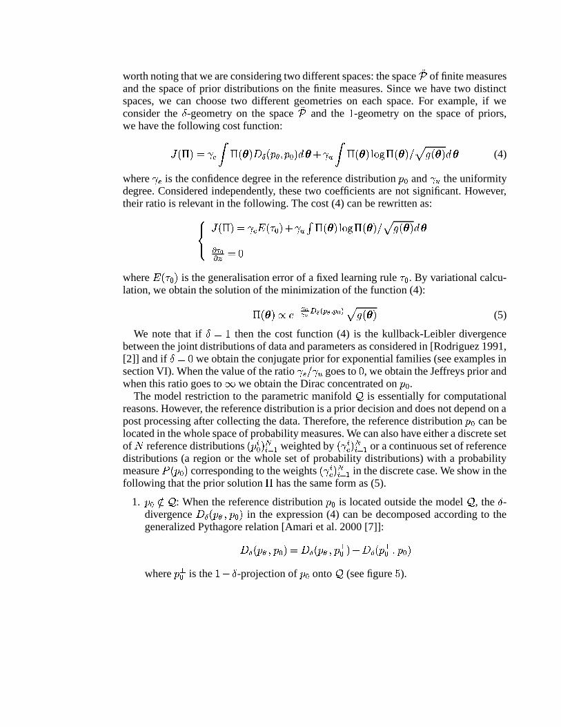
1. ��Ê �1ç% : When the reference distribution �èÊ is located outside the model % , the G -divergence dfeD�P� @ � �OÊ � in the expression (4) can be decomposed according to thegeneralized Pythagore relation [Amari et al. 2000 [7]]:d�e�� @ � ��Ê �=� d�eD�� @ � � ÅÊ � i d�eD�� ÅÊ � ��Ê �where � ÅÊ is the �g9hG -projection of �ËÊ onto % (see figure é ).

º¯

¢ Û¢�êÛ

��l e projection

Figure é . The equivalent of the non parametric reference distributionis its �g9hG projection onto the parametric model % .

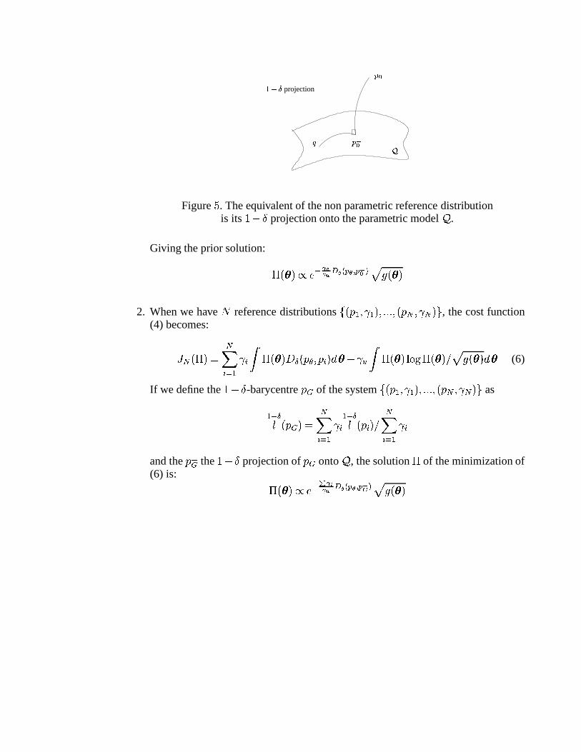
Giving the prior solution: A-� ��=SMÜ l Ý ÞÝ#àÓá Á â ¢�ã t ¢¦êÛ ä × p�� 2. When we have æ reference distributions & �P� �+� � ��+� ë¶ë�ë¶� �� "ì� � "í��* , the cost function

(4) becomes:Ñ " ��A �=� "î �P�� ¡ AB� �� d�e�� @ � � ��Âo i �ØÔ ¡ AB� ��Õ�ÖE© AB� �� Ë× p�� Âo (6)

If we define the �g9hG -barycentre �èï of the system & �P� �+� � ��+� ë¶ë�ë¶� �� "ì� � "0�+* as��l e� �P�Ëï �=� "î �P�� l e� �P� �� "î �P�� and the � Åï the ��9RG projection of �èï onto % , the solution A of the minimization of(6) is: A-� ��=SKÜ loð Ý#ñÝ à-á Á â ¢ ã t ¢ êò ä × p��

¢ òâ ¢�ó tõô ó ä��l e projection¢ êò¯º

â ¢Dö t¤ô ö äâ ¢�÷ t¤ô ÷ ä

Figure ø . The equivalent reference distribution is the �g9hG projectionof the �g9hG barycentre of the æ references distributions.

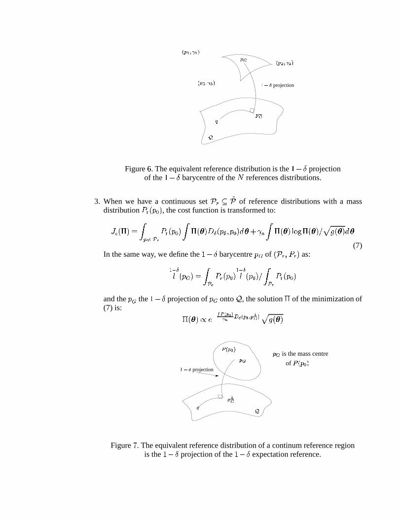
3. When we have a continuous set 5�ùûú �5 of reference distributions with a massdistribution ( ù��P��Ê � , the cost function is transformed to:Ñ\ü ��A �=� ¡ ¢ Û ¹ ¼\ý ( ù��P��Ê � ¡ AB� �� d�e�� @ � �OÊ ��Âo i �ØÔ ¡ AB� ��Õ�Ö�© AB� =� �Ë× p�� Âo

(7)In the same way, we define the �o92G barycentre ��ï of ��5$ù ��( ù � as:��l e� ��Ëï �=� ¡ ¼ ý ( ù��Ê � ��l e� �P��Ê � � ¡ ¼ ý ( ù��P��Ê �and the � Åï the ��9RG projection of �èï onto % , the solution A of the minimization of(7) is: AB� ��=SMÜ loþ U\V Z Û [Ý à á Á â ¢�ã t ¢ êò ä × p��

ÿ â ¢ Û�ä ¢ ò��l e projection ¢ êòº¯

�� is the mass centre

of ��

Figure . The equivalent reference distribution of a continum reference regionis the �o92G projection of the �o9hG expectation reference.

The above results show that whatever the choice of the reference distribution is, theresulting prior has the same form with a certain (non arbitrary) reference prior belongingto the model % . The existence of many reference distributions (or even a continuous set)indicates implicitly the existence of hyperparameter and the resulting solution shows thatthis hyperparameter is integrated and at the same time optimized if the a priori average(the barycentre) is considered as an optimization operation.

III. -FLAT FAMILIES

In this section we study the particular case of G -flat families. % is a G flat manifold if andonly if there exists a coordinate system |X�� such that the connection coefficients roeD� ��are null. We call |X�D�� an affine coordinate system. It is known that G -flatness is equivalentto ��96G flatness. Therefore, there exist dual affine coordinates |��\�� such that r ��l e�� è� � .One of the many properties of G -flat families is that we can express, in a simple way, theG -divergence dfe as a function of the coordinates and and thus any decision can becomputed while manipulating the real coordinates. It is shown in [Amari 1985, [3]] thatthe dual affine coordinates |��D�� and |�� are related by Legendre transformations and thecanonical divergence is: d�eD�� < �=�� P� � i � ��< � 9 �¥� �� )� ��< �where � and

�are the dual potentials such that:wxXy Ú��Ú+@ ñ � p �Xs Ú+@ ñÚ�� p l��Xs~E��)� ~E� � �K�¥�

For example, the exponential families are � -flat with the canonical parameters as � -affine coordinates, the mixture family is � -flat with the mixture coefficients as � -affinecoordinates, �5 �Ì& � � N ��çå * is G flat for all Gì1 |�� .

optimal estimates in flat families

As indicated in section II, the G optimal estimate is the G projection of N @ � e ( � �� which is the minimizer of the functional N @ ( � �� d�e�� @ � < � . We see that, in general,the divergence as a function of the parameters |�� has not a simple expression. However,with G -flat manifolds, we obtain an explicit solution. Noting that:~\� dfeD�P� @ � < �=� d�e�� @ � � ~E�� ¯ �=�K�¥� ��< � 9 �¥� �� the solution is: ®< � <F� ® �� ® � ¡ �( � �� nÂg f�Kz @�� £ |õ è�

This means that the G optimal estimate is the a posteriori expectation of the G affinecoordinates. Since the only degree of freedom of the affine coordinates is the affinetransformation, this estimate is invariant under affine reparameterization.

Noting also that: ~E� d ��l eD�P� � < �=� d ��l eD�P� � � ~E�� ¯ �=��)� ��< � 9 �� Then the a posteriori expectation of the ��9�G affine coordinates is the ��9�G optimalestimate.

Prior selection with flat families

The G prior A has the following general expression:A-� ��=SMÜ l Ý ÞÝ#àÓá Á â ¢�ã t ¢ Û�ä × p�� where ��Êk1Ì% is the equivalent reference distribution in the manifold % . When weassume that % is G flat with affine coordinates |X�� and dual affine coordinates |�� , theexpression of the prior becomes:A-� =�=S3Ü l}Ý#ÞÝ#à �� â { ä l @ ñ � Ûñ � × p�� E�where |�� Ê� � and |�� Ê� � are the affine coordinates of �ËÊ .

Therefore, we have an explicit analytic expression of the prior.In the Euclidean case, that is when the connection q is equal to its dual connection q v ,

which is equivalent to equality of the affine coordinates |X��M|�� , the G prior distributionis Gaussian with mean Ê and precision Q ô Þô à :AB� �E�=SMÜ l Ý ÞÝ#à�� {�lØ{ Û � ó

We detail here the notion of prior projection in the particular case of q v -autoparallelsubmanifolds % ��J³% . % � is ��g9hG � -autoparallel in % if and only if, at every point �61%!� , the covariant derivative q vÚ#" ~%$ remains in the tangent space & ¢ of the submanifold%!� at the point � . A simple characterization in flat manifolds is that the �n�}9 G � -affinecoordinates |�'Ë�� of % � form an affine subspace of the coordinates |��E�� . We can show thatby a suitable affine reparametrization of % , the submanifold %(� is defined as:wx y %!� �Ì& � � 1L%L� *) � Ê) is fixed *+ J & � ë¶ë � *where ��9M + is the dimension of %,� . If we consider the space % ü� such the comple-mentary dual affine coordinates )#) �M Ê)�) are fixed (

+%+ �,& � ë¶ë � * 9 + ), then the tangentspaces & ¢ and & ü¢ at the point �� Ê) �� Ê)#) � are orthogonal. Consequently, the projectedprior from % onto % � is simply:A Å �� =� ¡ ¯�¹�º.-" AB��< �=� ¡ @0/ AB� ) �� )#) ��Âo )

Hence, we see that the projected prior onto a q v -autoparallel manifold is the marginal-ization in the G affine coordinates and not in with respect to the 1) coordinates as itseems intuitive at a first look. This is essential due to the dual affine structure of thespace �5 .

IV. MIXTURE OF -FLAT FAMILIES AND SINGULARITIES

The mixture of distributions has attracted a great attention in that it gives a widerexploration of the probability distributions space based on a simple parametric manifold.For instance, by the mixture of Gaussians (which belongs to a � -flat family) we canapproach any probability distribution in total variation norm. In this section, we studythe general case of the mixture of G flat families. The space can be defined as:wxXy % � & � @ ¤� @ �32 us ��54 s � s � ë76� s �+*� s 1L% s�� % s is G flat

where the manifolds % s are either distinct or not.The mixture distribution can be viewed as an incomplete model where the weighted

sum is considered as a marginalization over the hidden variable ± representing the labelof the mixture. Thus � @ �82:9 ��± � ��<;k�± �� 9 � and the weights ��± � are the parameters ofa mixture family. We consider now the statistical learning problem within the mixturefamily. A mixture of G flat families is not, in general, G flat. Therefore the G optimalestimates have no more a simple expression. However, with data augmentation proce-dure we can construct iterative algorithms computing the solution. Here, we focus onthe computation of the G prior of the mixture density.

The G prior has the following expression:A-� ��=SMÜ l Ý ÞÝ#àÓá Á â ¢�ã t ¢ Û�ä × p�� (8)

The mixture (marginalization) form of the distribution � @ leads to a complex expressionof the G divergence and the determinant of the Fisher information. However, the com-putation of these expressions in the complete data distribution space [Rodriguez 2001,[8]] is feasible and gives explicit formula. By complete data � , we mean the union ofthe observed data � and the hidden data � . Therefore, the divergence will be consideredbetween complete data distributions:

d�e�� ü � � üÊ �� N�� ü�o92G i N$� üÊG 9 N4�P� ü � e �P� üÊ � ��l eGF��g9hG �where � ü is the complete likelihood ��; � ±$ �� and includes the parameters of theconditionals ��<;k�± �ß� 9 � and the discrete probabilities ��± � .

The additivity property of the G -divergence is not conserved unless G is equal to � or� [Amari1985, [3]]: d�e��P� � �>= � < � <?= �=� d�e��P� �+� < � � i d�e��>= � <?= � 9G��n�o9hG � dfeD�P� �� < � � d�e��P�@= � <A= �Consequently, in the special case of G²1 &)�m� � * , we have the following simple formula:wBBx BBy d�Ê�� Ê ��82 us ��C4 ÊsED d�Ê)�� s�� Ês � i Õ�ÖE©GF Û�F ��Hd � �� Ê ��82 us ��C4 s D d � �� s�� Ês � i Õ�Ö�© F �F Û� H

Singularities with mixture families

It is known that in learning the parameters of Gaussian mixture densities [Snoussi2001] the maximum likelihood fails because of the degeneracy of the likelihood functionto infinity when certain variances go to zero or certain covariance matrices approach theboundary of singularity. In [Snoussi 2001, [9]], there is an analysis of the occurrenceof this situation in the multivariate Gaussian mixture case. In this section, we give ageneral condition leading to this problem of degeneracy occurring in the learning withinthe mixture of G flat families.

Let % a G flat manifold and |��D�� the natural affine coordinates and |��E�� the dual affinecoordinates. The two coordinate systems are related by Legendre transformation [Amari1985, [3]]: wxXy Ú��Ú+@ ñ � p �Xs Ú+@ ñÚ�� p l��Xs~E��)� ~E� � �K�¥�where ��p �!s¦� s �� ! µ�P�� ! µ is the Fisher matrix and � and

�are the dual potentials.

It is clear from the expression of the variable transformation between the two affinecoordinates that a singularity of the Fisher information matrix p leads to non differ-entiability in the transformation between and . A singularity of p means that thedeterminant of this matrix is zero. Therefore, it is interesting to study the behaviour ofthe dual divergence at the boundary of singularity and we will show in an example thatthe dual divergences may have different behaviour as the distribution � approaches theboundary of singularity.

To illustrate such behaviour, we take a Gaussian family &�I ��J �AK = � LJ21R· �MK 1R·�N *which is a Q -dimensional statistical manifold � -flat. The � -affine coordinates are andthe � -affine coordinates are given by the following expressions:wx y ��POQ ó �8� = � l��= Q ó�Ó�=� J � � = � J = i K = (9)

The corresponding Fisher information are: p�� E� S8KSR�� p�� F� S � � KSR (10)

The canonical divergence has the following expression:d�e¥�P� �� >= �=� d ��l eD�P�>= � � ��=�T� �� i � �P�>= � 9 �¥� �� )� �P�@= � (11)

where � and�

are the potentials given by:�� O ó= Q ó i Õ�ÖE©VU Q5W Kg� � � l��= 9 Õ�Ö�©XU Q5W K (12)

We see that the degeneracy occurs when the variance K goes to zero. A detailed studyof how this degeneracy occurs in the Gaussian mixture case is in [Snoussi 2001, [9]]and is reviewed in the example of the next section. Here we focus on the difference ofbehaviour of the two canonical divergences d4Ê and d � .

The expression of the G prior is:Aje SMÜ l á Á â ¢�ã t ¢ Û�ä × p�� E�Following the complete data procedure:Y AjÊ SMÜ l Ý ÞÝßà[Z F ñ Û�\ á Û â ¢ ñã t ¢ ñÛ ä N^]�_a`�b ñ Ûb ñ^c × p�� ed2�A ��SMÜ l}Ý ÞÝßà Z F ñ \ á ö â ¢ ñã t ¢ ñÛ ä N b ñb ñ Û c × p�� 0d2�The resulting prior is factorized and separated into independent priors on the componentsof the Gaussian mixture. Combining expressions of (9), (10), (11) and ( 12) we note thefollowing comparison of the � and � priors through their dependences on the varianceKØs : G �K� G � �f f�49�: ~ % �49�: ~ %AìÊ is g6� KShs Ü lÓu ÛaijQ ó� � A � is g � K = F � Ý �Ý#às �f f

Exponential Polynomial

where k , lEÊ are constant.We note that:

• For G �3� , the prior decreases to � when � approaches the boundary of singularity~ % with an exponential term leading to an inverse Gamma prior for the variance.• For G � � , the prior decreases to � when � approaches the boundary of singularity~ % with a polynomial term leading to a Gamma prior for the variance. We note

the presence of the parameter 4 � in the power term.

This kind of behaviour pushes us to use the � prior in that it is able to eliminate thedegeneracy of the likelihood function.

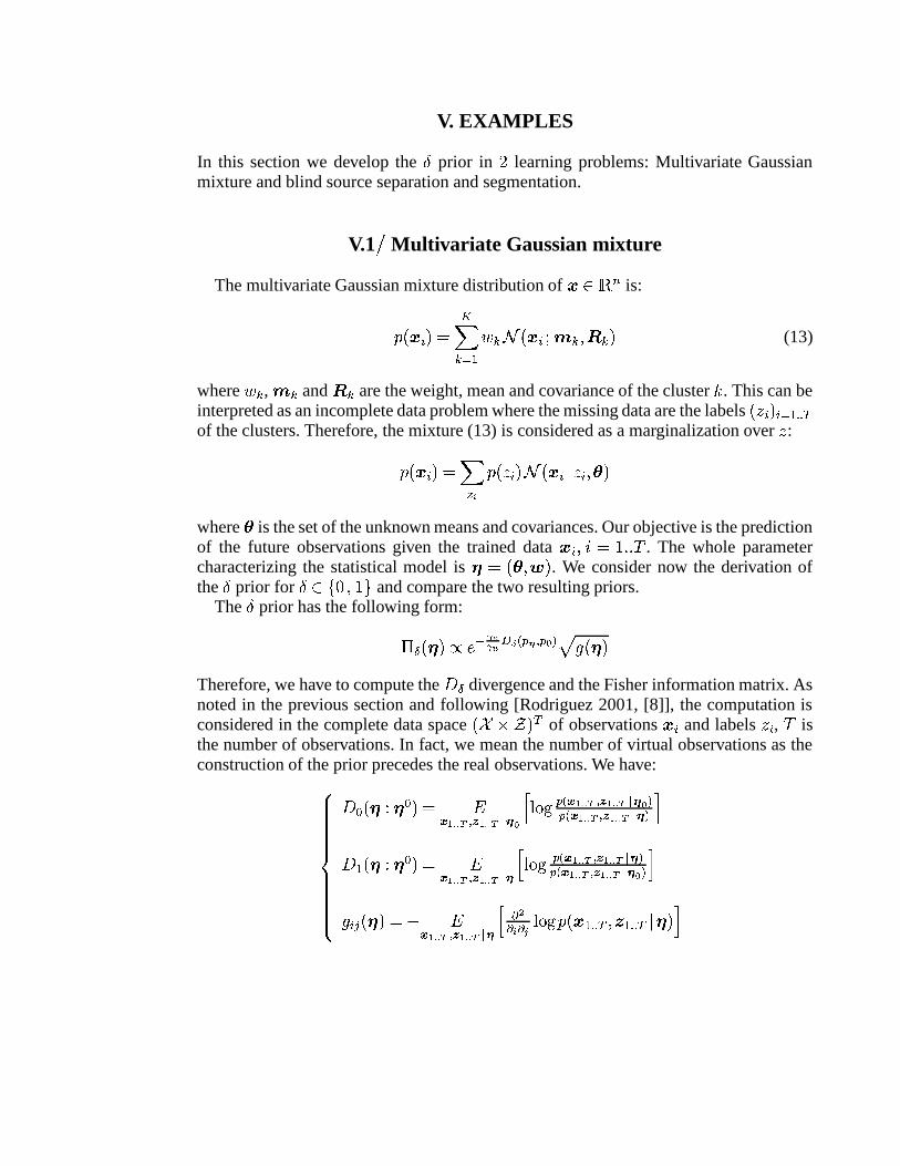
V. EXAMPLES

In this section we develop the G prior in Q learning problems: Multivariate Gaussianmixture and blind source separation and segmentation.

V.1 H Multivariate Gaussian mixture

The multivariate Gaussian mixture distribution of � 1 · µ is:

�� }�� mî u�� 4 u5I � �}�?6Mn³u��aoÎu�� (13)

where 4 u , n³u and oÎu are the weight, mean and covariance of the cluster l . This can beinterpreted as an incomplete data problem where the missing data are the labels �#± �� ! pof the clusters. Therefore, the mixture (13) is considered as a marginalization over ± :�� =� î 9 ñ ��#± ��qI � �� ± �� where is the set of the unknown means and covariances. Our objective is the predictionof the future observations given the trained data ��?r�� ë�ë�s . The whole parametercharacterizing the statistical model is � � o�0d2� . We consider now the derivation ofthe G prior for G²1 &)�� * and compare the two resulting priors.

The G prior has the following form:AìeD�� =SMÜ l Ý ÞÝ#àÓá Á â ¢ut t ¢ Û�ä × p�� Therefore, we have to compute the de divergence and the Fisher information matrix. Asnoted in the previous section and following [Rodriguez 2001, [8]], the computation isconsidered in the complete data space �evÉ�/ � p of observations �}� and labels ± � , s isthe number of observations. In fact, we mean the number of virtual observations as theconstruction of the prior precedes the real observations. We have:wBBBBBBBBx BBBBBBBBy

d�Ê)�� I7? Ê �=� zw ö�x x y t £ ö�x x y �{z Û D Õ�ÖE© ¢ â w ö�x x y t £ ö�x x y �|z Û ä¢ â w ö�x x y t £ ö�x x y �{z ä Hd � �� I7? Ê �=� zw ö�x x y t £ ö�x x y �{z D Õ�ÖE© ¢ â w ö�x x y t £ ö�x x y �{z ä¢ â w ö�x x y t £ ö�x x y �|z Û ä Hp �Xs �� =� 9 zw ö�x x y t £ ö�x x y �{z D Ú óÚ ñ Ú0� Õ�Ö�© �� í�� ! p�� ! p � � H

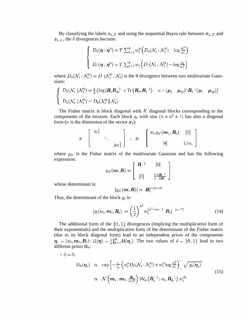
By classifying the labels � �� ! p and using the sequential Bayes rule between �� ! p and� �� ! p , the G divergences become:wBBx BBy d�Ê)�� I7M Ê �=�Ts 2 u�P�� 4 Ê�~} d�Ê)� Ih� 7 I Ê� � i Õ�ÖE© F ÛñF ñq�d � �� I7M Ê �=�Ts�2 u�P��4 � } d � � Ih� 7 I Ê� � i Õ�ÖE© F ñF Ûñ �where dfÊ�� I2� 7 I Ê� �� d � � I Ê� 7 Ih�� is the � divergence between two multivariate Gaus-sians:wxXy d�Ê�� Ih��CI Ê� �=� �=G� Õ�ÖE© oÎ��o l�� Ê i Tr � oÎ� Ê o l��T� 9R� i �0� � 9�� Ê � v o l�� 0� � 9�� Ê � �d � � Ih��CI Ê� �=� d�Ê)� I Ê� �CI2��

The Fisher matrix is block diagonal with � diagonal blocks corresponding to thecomponents of the mixture. Each block p � with size �� i � = i � � has also a diagonalform ( � is the dimension of the vector �� ):

p � �� | p �� . . . | p m �1�� p �m�� 4 � pA�� nÏ��Co �� |��|õ�� 4 � ��where p?� is the Fisher matrix of the multivariate Gaussian and has the followingexpression: pA�� n �aoh�� o l�� |õ�)�|X�� 9 �= Úq�� öÚA� ��whose determinant is: p?�� n �aoh� � o l â µ N@= äThus, the determinant of the block p � is:

p � � 4 �ß�en,�ß�ao �� Q�� µó 4 â µ ó N µ l�� ä� o � l â µ N@= ä (14)

The additional form of the &)�� * divergences (implying the multiplicative form oftheir exponentials) and the multiplicative form of the determinant of the Fisher matrix(due to its block diagonal form) lead to an independent priors of the components � � � 4 ��0n,��joÎ�� : AB�< �� mu�� A-�� . The two values of G ��&)�� * lead to twodifferent priors Aìe :

• G �¸� : AìÊ��< � � S �q�.� D 9 ô Þô à } 4 Ê� d�Ê�� I2� 7 I Ê� � i 4 Ê� Õ�ÖE© F ÛñF ñ � H × p � �< � � S I } n,��6Mn Ê � � ñh F Ûñ �� µ � o l�� 6C� Ê �ao l��Ê � 4¡ Û� (15)

with, k � ô Þô à �¢� Ê � k 4 Ê� �¤£ Ê � k 4 Ê� i µ ó N µ l��=� µ is the wishart distribution of an �6�� matrix:� µ � o¥65�m��¦B�=S o L§ � V�¨�© ö [ó �u�.� D 9 � Q Tr � oª¦ l�� HThe � -prior is Normal Inverse Wishart for the mean and covariance � n �ß�ao �� andDirichlet for the weight 4 � , that is the conjugate prior.

• G � � : A � �� S �u�.� D 9 ô Þô à } 4 � d � � I2� 7 I Ê� � i 4 ��Õ�Ö�© F ñF Ûñ � H × p � �� S I } n,�C6?n Ê � � ñh F ñ��«� µ } o ��6 k 4 � 9�� h F ñ l��h F ñ o Ê �4 ¨ ó ©C¨ � öó l â � N ¨ ó ä h F ñ� � 4 Ê� � h F ñ r µ � h F ñ l��= �

(16)

where r µ is the generalized Gamma function of dimension � ([6] page ÃØQ� ):r µ �� ¬ r�� Q �a®

öó µ â µ l�� ä µ¯ �P�� r��#� i r 9h�Q �� G° � 9��QThe � -prior A � (16) is the generalized entropic prior [Rodriguez 2001, [8]] to the

multivariate case. We see that the prior A � is a Wishart function of the covariancematrices oÎ� and the prior AìÊ is an inverse Wishart function of the covariances. Thisleads to a difference of the behaviour of these functions on the boundary of singularity(the set of singular matrices).

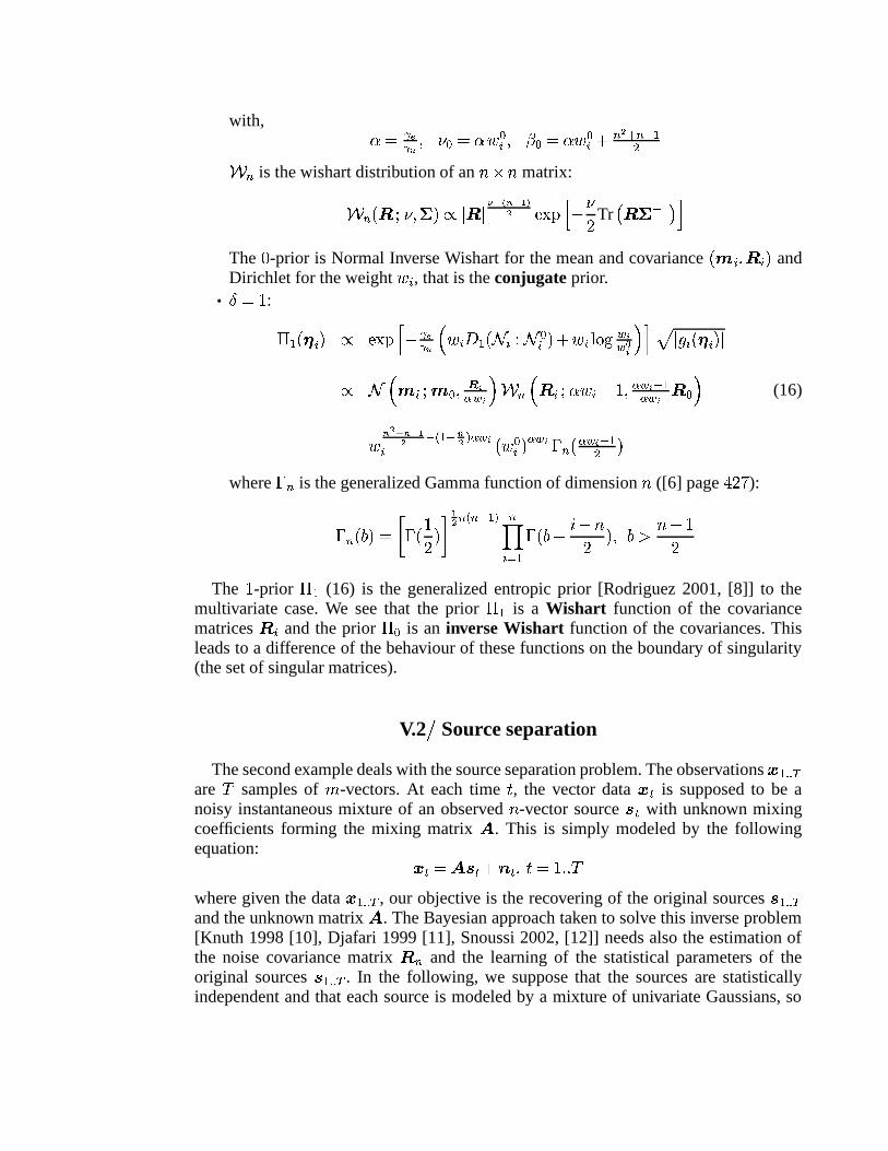
V.2 H Source separation

The second example deals with the source separation problem. The observations �ì�� ! pare s samples of ± -vectors. At each time ² , the vector data �1� is supposed to be anoisy instantaneous mixture of an observed � -vector source ³ � with unknown mixingcoefficients forming the mixing matrix � . This is simply modeled by the followingequation: ��O� ��³ � iª´ �� ² � � ë¶ë�swhere given the data �� ! p , our objective is the recovering of the original sources ³ �� ! pand the unknown matrix � . The Bayesian approach taken to solve this inverse problem[Knuth 1998 [10], Djafari 1999 [11], Snoussi 2002, [12]] needs also the estimation ofthe noise covariance matrix o µ and the learning of the statistical parameters of theoriginal sources ³ �� ! p . In the following, we suppose that the sources are statisticallyindependent and that each source is modeled by a mixture of univariate Gaussians, so

that we have to learn each set of source µ parameters s which contains the weights,means and variances composing the mixture µ :wxXy s � � s � � �P�� ! m � s � � � 4 s� � ± s � �eK s� �The index µ indicates the source µ and r indicates the Gaussian component r of thedistribution of the source µ . Therefore we don’t have a multidimensional Gaussianmixture but instead independent unidimensional Gaussian mixtures.

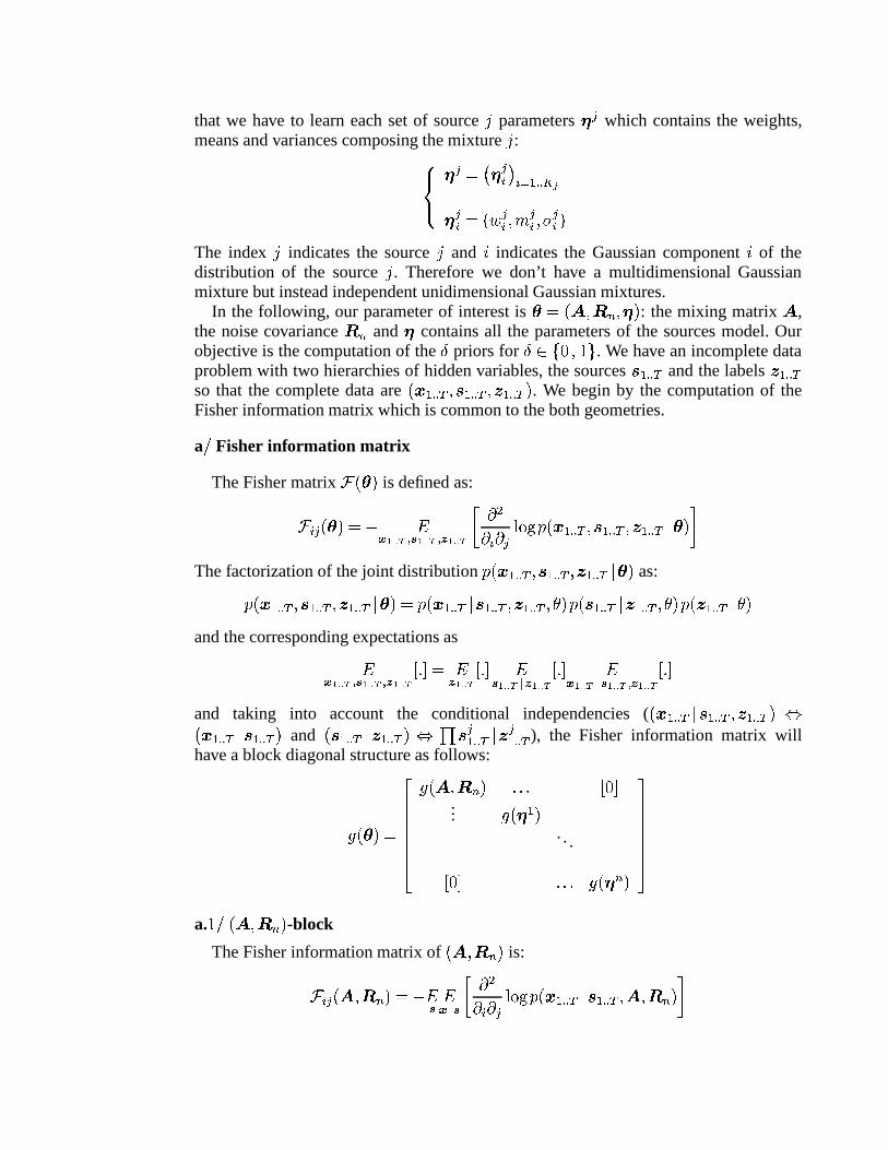
In the following, our parameter of interest is � �ß� �ao µ � � : the mixing matrix � ,the noise covariance o µ and contains all the parameters of the sources model. Ourobjective is the computation of the G priors for Gû1 &)�� * . We have an incomplete dataproblem with two hierarchies of hidden variables, the sources ³ �� ! p and the labels � �� ! pso that the complete data are � �� ! p�� ³ �� ! p�� ! p�� . We begin by the computation of theFisher information matrix which is common to the both geometries.

a � Fisher information matrix

The Fisher matrix ¶T� �� is defined as:¶ �Xs � ��=� 9 zw ö�x x y t · ö�x x y t £ ö�x x y ¬ ~ =~E��~�s Õ�ÖE© �� í�� ! p�� ³ �� ! p�� ! p �� ®The factorization of the joint distribution �� ! p�� ³ �� ! p�� ! p �� as:�� í�� ! p�� ³ �� ! p�� ! p ��=� �� $�� ! p <³ �� ! p�� ! p��E� ��e³ �� ! p �� ! p�� #� �� ! p ��and the corresponding expectations aszw ö�x x y t · ö�x x y t £ ö�x x y |PëX�m� z£ ö�x x y |�ë�� z· ö�x x y � £ ö�x x y |PëX� zw ö�x x y � · ö�x x y t £ ö�x x y |PëX�and taking into account the conditional independencies ( � �j�� ! p �³ �� ! p�� ! p��¸� �í�� ! p �³ �� ! p�� and �0³ �� ! p �� ! p��«¸ � ³ s �� ! p �� s �� ! p ), the Fisher information matrix willhave a block diagonal structure as follows:

p�� =� �¹¹¹¹¹�p��#� �jo µ � ë�ë ë |X��

... p�� . . .|X�� ë�ë ë p��< µ �

�»ººººº�a. � � �ß� �ao µ � -block

The Fisher information matrix of �#� �jo µ � is:¶ �Xs �#� �jo µ �=� 9 z · zw � · ¬ ~ =~\��~)s Õ�ÖE© �� í�� ! p �³ �� ! p=� � �ao µ � ®

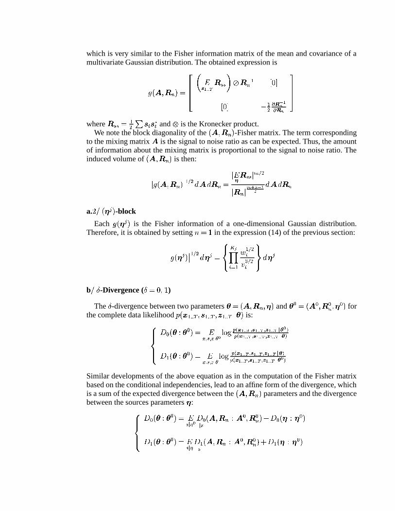
which is very similar to the Fisher information matrix of the mean and covariance of amultivariate Gaussian distribution. The obtained expression is

p��ß� �ao µ �=� �¹¹� � z· ö�x x y o�¼0¼ �¾½ o l��µ |X��|X�� 9 �= Úq� � ö¨Úq� ¨ �»ºº�

where o�¼e¼�� p 2 ³ � ³ v� and ½ is the Kronecker product.We note the block diagonality of the �ß� �ao µ � -Fisher matrix. The term corresponding

to the mixing matrix � is the signal to noise ratio as can be expected. Thus, the amountof information about the mixing matrix is proportional to the signal to noise ratio. Theinduced volume of �#� �jo µ � is then:

p��ß� �ao µ � � i = Â � Â¿o µ � z z o�¼0¼ À i = o µ ÂÁ ©5¨�© öó Â � Â¿o µa. Q � �� s � -block

Each p�� s � is the Fisher information of a one-dimensional Gaussian distribution.Therefore, it is obtained by setting � � � in the expression (14) of the previous section:ÃÃ p��< s � ÃÃ � i = Â s � wx y m �¯ �P�� 4 � i =�Ä%Å i =� Æ�ÇÈ Â sb � G -Divergence ( G �K�m� � )

The G -divergence between two parameters �� ß� �ao µ � � and Ê � �ß� Ê �ao Êµ � Ê � forthe complete data likelihood �� ! p=� ³ �� ! p�� ! p �� is:wBBx BBy d�Ê)� 7 Ê �=� zÉ t ¼�t 9 � @ Û Õ�ÖE© ¢ â w ö�x x y t · ö�x x y t £ ö�x x y � { Û ä¢ â w ö�x x y t · ö�x x y t £ ö�x x y � { äd � � 7 Ê �=� zÉ t ¼�t 9 � @ Õ�ÖE© ¢ â w ö�x x y t · ö�x x y t £ ö�x x y � { ä¢ â w ö�x x y t · ö�x x y t £ ö�x x y � { Û äSimilar developments of the above equation as in the computation of the Fisher matrixbased on the conditional independencies, lead to an affine form of the divergence, whichis a sum of the expected divergence between the �ß� �ao µ � parameters and the divergencebetween the sources parameters :wBBx BBy d�Ê�� 7 Ê �=� z¼ � � Û d�Ê� ¼ �ß� �ao µ 7�� Ê �ao Êµ � i d�Ê�� 7> Ê �

d � � 7 Ê �=�³z¼ � � d �� ¼ �ß� �ao µ 7è� Ê �ao Êµ � i d � �� Ï7> Ê �

where d�e� ¼ means the divergence between the distributions �� ! p �� ao µ � ³ �� ! p�� and�� $�� ! p �� Ê �jo Êµ � ³ �� ! p�� keeping the sources ³ �� ! p fixed.The G -divergence between and Ê is the sum of the G -divergences between each

source parameter s and s Ê due to the a priori independence between the sources. Then,the divergence between s and s Ê is obtained as a particular case ( � � � ) of the generalexpression derived in the multivariate case. Therefore we have the same form of the prioras in equations (15) and (16).

The expressions of the averaged divergences between the �#� �jo µ � parameters are:wBBBBBBBBBBx BBBBBBBBBByz¼ � � Û d�Ê� ¼ �#� �jo µ 7è�ÎÊ �ao µ Ê �=� �=~� Õ�ÖE© ÃÃ o µ o l��µ Ê ÃÃ i Tr � o l��µ o µ Ê �

i Tr ��o l��µ �#� 92�ÎÊ ��z¼ � � Û |{oÊ¼e¼�� ß�'92�RÊ � v � �z¼ � � d �� ¼ �#� �jo µ 7è�ÎÊ �ao µ Ê �=� �=~� Õ�ÖE© o µ Ê o l��µ i Tr � o l��µ Ê o µ �i Tr � o l��µ Ê �#� 92�ÎÊ �¥z¼ � � |{oÊ¼e¼�� #�'9 �ÎÊ � v � �

leading to the following G priors on �ß� �ao µ � :wBBBx BBBy AjÊ��ß� �ao l��µ � S I } � 6 �RÊ � �h o Ê ¼e¼ l�� ½ o µ � � � À } o l��µ 6 k �ao Êµ l�� z¼ � � ||o�¼0¼�� Á óA � �ß� �ao µ � S I � � 6 �ÎÊ � �h z¼ � � ||o�¼0¼�� l�� ½ o Êµ � � � À � o µ 6 k�9R� � h l µh o Êµ �

Therefore, the � -prior is a normal inverse Wishart prior (conjugate prior). The mixingmatrix and the noise covariance are not a priori independent. In fact, the covariancematrix of � is the noise to signal ratio

�h o Ê ¼e¼ l�� ½ o µ . We note a multiplicative termwhich is a power of the determinant of the a priori expectation of the source covariancez¼ � � ||o�¼0¼�� . This term can be injected in the prior �� and thus the �#� �jo µ � parameters and

the parameters are a priori independent.The � -prior (entropic prior) is normal Wishart. The mixing matrix and the noise

covariance are a priori independent since the noise to signal ratio�h z¼ � � ||oÊ¼e¼�� l�� ½ o Êµ

depend on the reference parameter o Êµ . However, we have in counterpart the dependenceof � and through the term z¼ � � |{oÊ¼e¼�� l�� present in the covariance matrix of � . In practice,

we prefer to replace the expected covariance z¼ � � |{oÊ¼e¼�� , in the two priors, by its reference

value o Ê ¼e¼ .We note that the precision matrix for the mixing matrix � ( k o Ê ¼e¼ ½ o l��µ for AjÊ

and k z¼ � � ||o�¼0¼�� ½ o Êµ l�� for A � ) is the product of the confidence term k � ô Þô à in the

reference parameters and the signal to noise ratio. Therefore, the resulting precision

of the reference matrix �hÊ is not only our a priori coefficient �FÒ but the product of thiscoefficient and the signal to noise ratio.

VI. CONCLUSION AND DISCUSSION

In this paper, we have shown the importance of providing a geometry (a measure ofdistinguishibility) to the space of distributions. A different geometry will give a differentlearning rule mapping the training data to the space of predictive distributions. Theprior selection procedure established in a statistical decision framework needs to betaken in a specified geometry. We have tried to elucidate the interaction between theparametric and non parametric modeling. The notion of "projected mass" gives to therestricted parametric modelization a non parametric sense and shows the role of therelative geometry of the parametric model in the whole space of distributions. The sameinvestigations are considered in the interaction between a curved family and the wholeparametric model containing it. Exact expressions are shown in a simple case of auto-parallel families and we are working on the more abstract space of distributions.

REFERENCES

1. R. E. Kass and L. Wasserman, “Formal rules for selecting prior distributions: A review and annotatedbibliography”, Technical report no. 583, Department of Statistics, Carnegie Mellon University, 1994.

2. C. Rodríguez, “Entropic priors”, Tech. rep. Electronic form http:omega.albany.edu:8008/entpriors.ps, (1991).

3. S. Amari, Differential-Geometrical Methods in Statistics, Volume 28 of Springer Lecture Notes inStatistics, Springer-Verlag, New York, 1985.

4. H. Zhu and R. Rohwer, “Bayesian invariant measurements of generalisation”, in Neural Proc. Lett.,1995, vol. 2 (6), pp. 28–31.

5. H. Zhu and R. Rohwer, “Bayesian invariant measurements of generalisation for continuous dis-tributions”, Technical report, NCRG/4352, ftp://cs.aston.ac.uk/neural/zhuh/continuous.ps.z, AstonUniversity, 1995.

6. G. E. P. Box and G. C. Tiao, Bayesian inference in statistical analysis, Addison-Wesley publishing,1972.

7. S. Amari and H. Nagaoka, Methods of Information Geometry, vol. Volume 191 of Translations ofMathematical Monographs, AMS, OXFORD, University Press, 2000.

8. C. Rodríguez, “Entropic priors for discrete probabilistic networks and for mixtures of Gaussiansmodels”, in Bayesian Inference and Maximum Entropy Methods, R. L. FRY, Ed. MaxEnt Workshops,August 2001, pp. 410–432, Amer. Inst. Physics.

9. H. Snoussi and A. Mohammad-Djafari, “Penalized maximum likelihood for multivariate gaussianmixture”, in Bayesian Inference and Maximum Entropy Methods, R. L. Fry, Ed. MaxEnt Workshops,August 2002, pp. 36–46, Amer. Inst. Physics.

10. K. Knuth, “A Bayesian approach to source separation”, in Proceedings of Independent ComponentAnalysis Workshop, 1999, pp. 283–288.

11. A. Mohammad-Djafari, “A Bayesian approach to source separation”, in Bayesian Inference andMaximum Entropy Methods, J. R. G. Erikson and C. Smith, Eds., Boise, IH, July 1999, MaxEntWorkshops, Amer. Inst. Physics.

12. H. Snoussi and A. Mohammad-Djafari, “MCMC Joint Separation and Segmentation of HiddenMarkov Fields”, in Neural Networks for Signal Processing XII. IEEE workshop, September 2002,pp. 485–494.

Documents

Information geometry and prior selectionomega.albany.edu:8008/ignorance/snoussi02.pdf · Information geometry and prior selection Hichem Snoussi and Ali Mohammad-Djafari Laboratoire