Information Frictions and Adverse Selection: Policy

Information Frictions and Adverse Selection:

Policy Interventions in Health Insurance Markets∗

Benjamin R. HandelUC Berkeley and NBER

Jonathan T. KolstadUC Berkeley and NBER

Johannes SpinnewijnLondon School of Economics and CEPR

January 29, 2016

Abstract

A large literature has analyzed pricing inefficiencies in health insurance markets due to adverseselection, typically assuming informed, active consumers on the demand side of the market.However, recent evidence suggests that many consumers have information frictions that lead tosuboptimal health plan choices. As a result, policies such as information provision, plan recom-mendations, and smart defaults to improve consumer choices are being implemented in manyapplied contexts. In this paper we develop a general framework to study insurance market equi-librium and evaluate policy interventions in the presence of choice frictions. Friction-reducingpolicies can increase welfare by facilitating better matches between consumers and plans, butcan decrease welfare by increasing the correlation between willingness-to-pay and costs, exac-erbating adverse selection. We identify relationships between the underlying distributions ofconsumer (i) costs (ii) surplus from risk protection and (iii) choice frictions that determinewhether friction-reducing policies will be on net welfare increasing or reducing. We extend theanalysis to study how policies to improve consumer choices interact with the supply-side policyof risk-adjustment transfers and show that the effectiveness of the latter policy can have impor-tant implications for the effectiveness of the former. We implement the model empirically usingproprietary data on insurance choices, utilization, and consumer information from a large firm.We leverage structural estimates from prior work with these data and highlight how the model’smicro-foundations can be estimated in practice. In our specific setting, we find that friction-reducing policies exacerbate adverse selection, essentially leading to the market fully unraveling,and reduce welfare. Risk-adjustment transfers are complementary, substantially mitigating thenegative impact of friction-reducing policies, but having little effect in their absence.

∗We thank Glen Weyl for his extensive comments on the paper. We thank Dan Ackerberg, Hunt Alcott,Saurabh Bhargava, Liran Einav, Amy Finkelstein, Avi Goldfarb, Josh Gottlieb, Matt Harding, Neale Mahoney,Josh Schwartzstein, Justin Sydnor, Dmitry Taubinsky, and Mike Whinston for their comments. We also thankseminar participants at Arizona State, The Becker Friedman Price Theory Conference, CEPR, CESifo, Minnesota,Princeton, UCLA, the 2015 Yale Marketing-Industrial Organization Conference, and the ASSA Annual Meetings.We thank Zarek Brot-Goldberg for outstanding research assistance. We thank Microsoft Research for their supportof this work.

1

1 Introduction

A central goal of policy in health insurance markets is to set up an environment whereby firms will

offer, and consumers can purchase, efficient insurance products that meet consumer demands for

risk protection and health care provision. One key impediment to achieving this goal is adverse

selection resulting from sicker consumers purchasing more comprehensive coverage and, ultimately,

driving up premiums, [see e.g. Akerlof (1970) or Rothschild and Stiglitz (1976)]. The extent

of adverse selection within a given insurance market can be impacted by a variety of policies

including constraints on the types of contracts offered [as in the Affordable Care Act (ACA)],

premium subsidies [Einav et al. (2010b)], premium risk rating [Bundorf et al. (2012), Handel et al.

(2015)], mandates to purchase coverage [e.g. Hackmann et al. (2015)] and risk-adjustment transfers

[Cutler and Reber (1998), Handel et al. (2015)]. Work to assess these policy options assumes that

consumers have full information regarding the different aspects of their plan choice or, put slightly

differently, that the choices consumers make reflect their true plan valuations that are relevant to

policy analysis. However, a collection of recent empirical research on consumer choices in health

insurance markets supports the notion that consumers may be far from fully informed about their

health plan choices, and may have difficulties making decisions under limited information [see e.g.

Handel and Kolstad (2015b), Ketcham et al. (2012), Abaluck and Gruber (2011), Barseghyan et

al. (2013), Bhargava et al. (2015) and Kling et al. (2012)].1 Accordingly, policy interventions in

insurance markets to reduce consumer choice frictions such as, e.g., information provision, plan

recommendations, or smart defaults are being widely considered and, increasingly, implemented

[see e.g. Handel and Kolstad (2015a)].

Despite the policy relevance of information frictions and the large amount of work analyzing

insurance market policies, there is still limited theoretical and empirical work systematically ana-

lyzing market policies and welfare in the context of consumers with limited information or imperfect

decision making. In this paper we develop a general theoretical model to investigate the interac-

tions between demand and supply-side inefficiencies in health insurance markets, caused by choice

frictions and adverse selection respectively. The model extends prior work by Spinnewijn (2015) in

several key directions, and also builds on prior work by Einav et al. (2010a) and Veiga and Weyl

(2015). We use the model to ask whether friction-reducing policies will increase or decrease welfare

in a given applied setting, and answer this question by linking specific characteristics of the under-

lying population distributions of key micro-foundations to these normative consequences. While

prior empirical work on inertia and adverse selection [e.g. Handel (2013) and Polyakova (2015)]

highlights specific cases where reduced frictions can lead to welfare losses, this is the first work we

are aware of that develops a general framework to assess when we should expect friction-reducing

policies to be welfare increasing or decreasing based on key sufficient micro-foundations in selection

1Past work that shows consumers may have limited information does not necessarily presume that consumers aremaking poor choices from an ex ante search perspective. It is plausible that acquiring information about healthinsurance given a specific choice architecture is quite costly and consumers make rational information acquisitiondecisions leading to limited information. Alternatively, consumers could have problems processing the informationthat they have or problems making information acquisition decisions.

2

markets. To show how our framework can be applied in practice, we implement it empirically using

the data and estimates developed in Handel and Kolstad (2015b), who study insurance choice and

design in a large employer context.

Our model characterizes how information frictions (and the policies that impact them) affect

equilibrium outcomes and welfare in two classes of insurance markets studied in the literature.

These include (i) those where insurers compete to offer supplemental coverage relative to a publicly

provided baseline plan [see e.g. Einav et al. (2010b)] or (ii) those where insurers compete to offer

two types of insurance plans characterized by financial generosity [see e.g. Handel et al. (2015)]

in a market with an enforced individual mandate.2 While this setup abstracts away from issues

of imperfect competition, which are empirically relevant in many insurance market contexts, we

believe that these two classes of competitive markets are natural starting points for thinking about

the general implications of friction-reducing policies in selection markets.3

For these market environments, we model the primitives of (i) consumer willingness-to-pay (ii)

the impacts of consumer frictions on willingness-to-pay (iii) consumer costs and (iv) consumer

surplus from risk protection.4 We map these foundations into demand, cost, and welfare-relevant

value curves, and use these objects to study positive and normative market outcomes under different

policies.5 We develop simple expressions to characterize the marginal impact of a policy change

in terms of means and variances of the demand primitives (i.e., cost, surplus and friction value)

among the marginal consumers. When frictions push the marginal consumers to demand more

(less) generous coverage on average, a friction-reducing policy works like a tax (subsidy), which

would be undesirable (desirable) when due to adverse selection equilibrium coverage is inefficiently

low. In addition to this level effect on the willingness to pay, frictions also impact the sorting of

consumers, (i) affecting the match between consumers and plans conditional on equilibria prices

and (ii) changing the equilibria prices by changing the correlation between costs and willingness-to-

pay. We prove results showing that the relationship between the underlying means and variances of

consumer surplus and expected yearly costs in the population are crucial for determining whether

friction-reducing policies will have positive or negative welfare impacts (conditional on a given

distribution of underlying frictions). As the mean and variance of surplus rise relative to those of

costs, friction-reducing policies become more attractive: the benefits of facilitating better matches

2See Weyl and Veiga (2015) for an in depth discussion of the equilibrium properties of the two classes of regulatedcompetitive markets we study here.

3See Mahoney and Weyl (2014) for an analysis of selection markets with imperfect competition, which reversessome typical policy conclusions from competitive selection markets.

4Our analysis assumes that consumers benefit from incremental risk protection, but that there is no correspondingsocial benefit from reduced inefficient utilization (moral hazard), an important component of optimal insurancedesign that is oft-discussed in the literature. We make this assumption for simplicity: including moral hazardwould increase the welfare impact of consumers enrolling in less generous coverage (and reduce the welfare impactof adverse selection) but would not impact our key positive comparative statics related to information frictions andrisk-adjustment policies.

5For information frictions, the space of policies we consider reduces the impact of all frictions proportionally.Alternative specifications could include informing some specific proportion of consumers or informing consumersonly on one dimension. We abstract away from specific policies to inform consumers and their potential levels ofeffectiveness. This is in the spirit of the sufficient statistics literature where our parameters can reflect a range ofunderlying choice micro-foundations. We assume simply that such policies exist, and assess their impacts given theirexistence. See, e.g. Kling et al. (2012) for an empirical example of one such policy.

3

between consumers and plans in equilibrium begin to outweigh the costs of increased sorting on

costs and subsequent adverse selection. Conversely, as the mean and variance of costs increases

relative to surplus, friction-reducing policies become less attractive. We explore these theoretical

properties in a series of simulations designed to highlight these key effects.

In addition to characterizing when friction-reducing policies are ‘good’ or ‘bad’ on their own, we

study how these policies interact with the supply-side policy of insurer risk-adjustment transfers.

These transfers are designed to reverse adverse selection by compensating insurers who enroll ex

ante sicker consumers with transfers from insurers that enroll ex ante healthier consumers and are

present in many different contexts (e.g. ACA exchanges, Medicare Part D, Medicare Advantage).6

Thus, the combination of policies is a more appropriate characterization of market policies in

practice than either in isolation.

We model insurer risk-adjustment transfers by allowing the insurer average and marginal cost

curves to rotate as a function of the effectiveness of the risk-adjustment policy.7 We study two

features related to the interaction of friction-reducing policies and risk-adjustment policies. First,

we show that in adversely selected markets increased risk-adjustment strength improves the welfare

impact of friction-reducing policies, and can shift them from welfare-negative to welfare-positive.

Second, we show that as friction-reducing policies become less attractive (e.g. as the potential for

adverse selection increases) effective risk-adjustment plays a much more important role in increas-

ing welfare. These results illustrate the importance of coordinating demand-side interventions with

supply-side policies commonly used in insurance markets. We note that these underlying compara-

tive statics hold regardless of whether the market studied is for one priced supplemental plan or for

two priced plans that differ in generosity. However, as shown in Weyl and Veiga (2015), the market

with two priced plans is more likely to unravel in an environment with adverse selection.8 With

the insights in hand, we apply our framework to an empirical context where we can measure the

distributions of surplus from risk protection, costs, and the impact of frictions on willingness-to-pay.

This empirical analysis both highlights the impact the policies we study have in one context, and

illustrates how to apply our framework empirically in other contexts.

We apply our framework using empirical estimates from Handel and Kolstad (2015b) who

study proprietary data on the health plan choices and claims of over 35,000 employees (105,000

6See e.g. Cutler and Reber (1998), Brown et al. (2014) or Geruso and McGuire (2014) for discussions of risk-adjustment policies in the literature. See Kaiser Family Foundation (2011) for a discussion of these policies in thecontext of the ACA.

7Specifically, in our model the costs to the insurer for enrolling a given consumers equals that consumer’s actualexpected cost plus a risk-adjustment transfer that moves that cost by some proportion towards population averagecost. Thus, if there are no risk-adjustment transfers then costs equal that consumer’s specific expected costs to thatplan, while under full risk-adjustment transfers any consumer’s cost equals population average costs for that plan,from the insurer’s perspective.

8This occurs because generous plans are forced to internalize the full costs of insuring the sickest consumers (ratherthan their supplemental costs) while less generous coverage cost is based on the full costs of healthiest consumers.The price difference reflects this difference in average costs, rather than the average difference in supplemental costsfor those enrolling. Consequently, the market with two priced plans is more likely to unravel and friction-reducingpolicies are more likely to have a negative impact, while risk-adjustment is likely to be more important. The underlyingrelationships we study are unchanged, but a higher threshold is required for friction-reducing policies to be beneficialin the market with two priced plans. We investigate this both in simulations and in our empirical application.

4

employees and dependents) at one large firm, linked at the individual-level to a comprehensive

survey designed by the authors to measure the extent of consumers’ potentially limited information

on many dimensions relevant to health plan choice.9 Using this data, the authors estimate an

expected utility plan choice model that accounts for the effects of limited information on choice.

We use their estimates of risk preferences, health risk, and friction effects on choices to char-

acterize the non-parametric sample joint distributions of (i) consumer costs (ii) consumer surplus

from risk protection and (iii) the impact of consumer choice frictions on willingness-to-pay. For

a given insurance market setup, our model maps these primitives into demand, welfare-relevant

value, average cost, and marginal cost curves that permit us to characterize equilibrium price,

quantity, and welfare.10 We use these primitives in conjunction with our model to investigate the

positive and normative implications of (i) friction-reducing policies and (ii) additional supply-side

policies in our empirical context. While we make several assumptions to move from the large-

employer context these estimates come from to the competitive counterfactual markets studied in

our theoretical framework, these stylized assumptions allow us to illustrate the implications of the

policy combinations we consider for market equilibria and social welfare using data and empirical

estimates with appropriate depth and scope.

We estimate that consumers have a high mean ($1,787) and standard deviation ($1,304) of

the impact of frictions on willingness-to-pay (pushing consumers towards more generous coverage).

Expected family total costs are high, just over $10,000, as is the variance of costs, implying both

high mean and variance of the cost of providing more generous coverage. The mean and variance of

estimated surplus from incremental risk protection, however, are both low, reflecting low estimated

risk aversion. These foundations suggest that friction-reducing policies on their own will be welfare-

reducing, because the mean and variance of costs are high relative to those of surplus; informing

consumers on their underlying value from insurance will increase the role of cost in decision making,

exacerbating adverse selection, without substantially enhancing welfare by allocating people to the

plan that gives them more surplus.

We describe our results for the class of one competitively priced supplemental policy, and note

that, though more adversely selected, the market we analyze with two competitively priced policies

has similar comparative statics. In this counterfactual market without any policy interventions, 85%

of consumers enroll in more generous coverage with the remaining 15% in just the baseline option.

This implies limited under-insurance in our stylized counterfactual environment, where 100% of

consumers should enroll in more generous coverage.11 When the impact of frictions on willingness-

to-pay is reduced by 50% then 73% of consumers enroll in more generous insurance coverage in

9To protect the anonymity of the firm, we cannot reveal the exact number of employees and dependents.10This empirical work drawing a clear distinction between willingness-to-pay and the welfare-relevant valuation once

a product is allocated is in the spirit of recent work by Baicker et al. (2015) in health care purchasing, Bronnenberget al. (2014) in generic drug purchasing, Alcott and Taubinsky (2015) in lightbulb purchasing, Taubinsky (2016) fortax salience, and Bernheim et al. (forthcoming) in 401(k) allocations. See Dixit and Norman (1978) for a theoreticaldiscussion of the distinction between revealed preference and consumer welfare, in the context of advertising.

11While we assume away ‘moral hazard’ in consumer health purchasing, we note that including this would shift thewelfare impacts of being enrolled in less generous coverage, but not change the nature of the positive comparativestatics we study. See Brot-Goldberg et al. (2015) for a study of moral hazard in this empirical environment.

5

equilibrium. Removing frictions completely, however, leaves only 9% of enrollees in the generous

plan. Thus, while adverse selection is still fairly limited when frictions are partially removed, in our

environment fully removing those frictions substantially exacerbates adverse selection, essentially

leading to the market fully unraveling. We quantify the welfare impact of these friction reducing

policies, and find that the policy that reduces frictions by 50% reduces the share of first-best surplus

achieved to 57% and completely removing frictions reduces that share to 15%. From a distributional

standpoint, healthy consumers with frictions heavily pushing them towards comprehensive coverage

gain from the friction-reducing policy, but most consumers, especially the sickest ones, lose out from

the policy.

In our empirical analysis, risk-adjustment transfers are strongly complementary to friction-

reducing policies, since those policies cause the market to unravel. When there is no policy in

place to reduce frictions, risk adjustment transfers that are 50% (100%) effective increase cov-

erage from 84.6% to 87.1% (88.5%), a positive, but small impact on coverage. However, when

the policy to reduce frictions is fully effective, risk adjustment transfers that are 50% (100%) ef-

fective increase coverage from 9.1% to 51.6% (63.5%), with similar increases in the percent of

first-best surplus achieved. We present equilibrium and welfare under the full two-dimensional

space of friction-reducing and risk-adjustment policy effectivenesses, and generally show that risk-

adjustment transfers are very impactful in our environment when frictions are reduced, but less

impactful when they are present. Though the combined policy of fully-reduced frictions and fully-

effective risk-adjustment reduces welfare slightly relative to the status quo, from a distributional

standpoint there is greater equity, in the sense that there are fewer consumers leaving substantial

sums of money on the table given equilibrium prices.

Our paper proceeds as follows. In Section 2 we present our theoretical framework, characterize

market equilibrium and welfare and demonstrate how both are affected by demand-side and supply-

side policy interventions. We also present a range of simulations designed to highlight key features

of the model. Section 3 describes the data used in our analysis, and presents some simple descriptive

statistics. Section 4 describes the choice model estimated in Handel and Kolstad (2015b) and its

estimates. Section 5 discusses how we calibrate the model developed in Section 2 with the estimates

from Section 4. Section 6 presents our empirical analysis of market equilibrium, friction-reducing

policies, and insurer risk-adjustment policies. Section 7 concludes.

2 Theory

Here we develop a stylized model of the insurance market which allows us to analyze adverse

selection (or supply side pricing inefficiencies more generally) and information frictions among

consumers. We use our model to consider different policy options available in insurance markets

to address adverse selection (e.g. risk adjustment) and information frictions (e.g. consumer choice

tools). We extend the model to incorporate risk adjustment as this an important policy option

considered both in theory and in practical applications (including as a part of the ACA).

6

2.1 Setup

Our primary model considers the case where there is a competitive market for one priced insurance

plan, offered to all individuals in the market at price P . As discussed in Einav et al. (2010b),

this could, e.g., reflect a market for supplemental coverage above and beyond a publicly provided

government baseline coverage option. Individuals decide whether to buy the insurance plan or not.

An individual i’s willingness-to-pay for the plan equals wi. The expected cost of providing the

coverage depends on the individual’s health risk and is denoted by ci. Information frictions enter

the model as a distortion to individual’s willingness-to-pay. We denote the welfare-relevant value

of the plan for individual i by vi and the friction value by fi such that wi = vi + fi. An individual

buys the plan if her willingness-to-pay exceeds the premium, wi ≥ P , while she would maximize

her true utility by buying the plan if vi ≥ P . From a welfare perspective, however, it is efficient for

her to buy insurance only if the surplus is positive, si ≡ vi − ci ≥ 0.

Our model thus captures three sources of heterogeneity underlying the heterogeneity in insur-

ance choices,

wi = si + ci + fi.

Both the insurance cost c and the friction value f are inefficient drivers of insurance demand as

social welfare is maximized when all individuals with positive surplus buy insurance. We assume

that all variables underlying the heterogeneity are continuously distributed. The additivity of the

demand components is not restrictive when we do not impose constraints on the underlying joint

distribution. The model assumes that consumers have a zero price elasticity for health care spend-

ing, an oft-discussed parameter in the literature. We do this to focus the analysis on information

frictions, risk-adjustment, and adverse selection: incorporating estimates on price elasticity would

change the welfare numbers that result, but not the comparative statics we study.

In an expected utility framework, the value v corresponds to the difference between the certainty

equivalent of facing the distribution of total expenses and the certainty equivalent of facing the

distribution of out-of-pocket expenses when covered by insurance. The surplus s corresponds to the

difference in risk premia with and without the plan. The friction f corresponds to the difference in

willingness-to-pay as a result of, e.g., limited information or decision-biases at the time of purchase.

See, e.g., Dixit and Norman (1978) for a prior theoretical framework discussing the distinction

between demand and welfare-relevant value.

The model can be easily extended to a market where there are two classes of competitively priced

plans (high and low coverage), as studied in Handel et al. (2015). In that case, the different demand

components (surplus s, cost c and friction f) correspond to the additional coverage provided by

the high-coverage relative to the low-coverage plan, as in the empirical environment we study later.

We discuss this theoretical and empirical distinction further in Appendix D. See Weyl and Veiga

(2015) for further discussion of the differences between these two market setups. In our context,

the comparative statics we study are the same across these distinct setups, though of course actual

market outcomes differ.

7

Demand and Ordering Individuals with different characteristics will sort into insurance de-

pending on the price. The share of individuals buying insurance Q depends only on the distri-

bution of the willingness-to-pay w. That is, the demand for insurance at a premium P equals

D (P ) = 1 − G (P ), where G is the cdf of w. The price elasticity of demand equals εD (P ) =

−g (P )P/[1−G (P )].

The ordering of individuals, denoted by O, and in particular how individuals differ in their

characteristics when ordered according to their willingness-to-pay, is key for the analysis. The

gradient of the expected costs is crucial for the determination of the market equilibrium, while the

gradient of surplus determines the welfare generated in equilibrium. The presence of information

frictions affects the sorting of individuals and thus the respective gradients.12 Similarly, any policy

intervention that changes the ordering of individuals based on their willingness-to-pay will change

the sorting of individuals into insurance and thus affect equilibrium and welfare.

We introduce the notation EP (·) ≡ E (·|w = P ) and E≥P (·) ≡ E (·|w ≥ P ) to denote the

expected value among the marginal individuals (at the margin between buying insurance or not)

and the infra-marginal individuals (weakly preferring to buy insurance) respectively. The expected

values are conditional on the particular ordering of individuals O.

Equilibrium Since some characteristics of individuals cannot be observed or priced by insurance

companies, they care about the sorting of individuals into insurance based on their costs. In our

stylized model we assume that cost c is unobservable (or unable to be priced) and insurers only

compete on prices, taking all other features of the health plan as given.13

We focus our analysis on a competitive environment where the equilibrium price will reflect the

expenses made by all individuals buying the health plan. That is, the insurer makes a positive

profit as long as the premium P exceeds the average cost of providing insurance to the buyers of

insurance at that price, E≥P (c). Following Einav et al. (2010b) and Handel et al. (2015), we define

the competitive price P c by

P c = E≥P c (c) . (1)

The corresponding equilibrium coverage equals Qc = D (P c). The analysis can be extended to

imperfect competition, which introduces marginal revenues and marginal costs in the price setting

[see Mahoney and Weyl (2014)]. For example, a monopolist would set the price at a mark-up above

marginal costs, Pm = 11+1/εD(Pm)EP c (c).

Welfare Equilibrium welfare depends on the sorting of individuals into insurance based on sur-

plus. We consider the total surplus (value net of cost) generated in the insurance market to evaluate

welfare. This assumes that information frictions are not welfare-relevant once a consumer is allo-

cated to a given plan, an assumption we briefly discuss in our empirical context in Section 5. This

12This approach on the demand side is also similar in spirit to ongoing work by ? on tax salience.13See Veiga and Weyl (2015) and Azevedo and Gottlieb (2015) for an analysis of the plan features provided in

equilibrium.

8

also ignores distributional consequences of policy interventions, which we consider in the empirical

analysis in Section 6.

For a given ordering O and share Q of individuals buying insurance, welfare equals

W(Q,O) =

∫P≥P

EP (s) dG(P ) = [1−G (P )]× E≥P (s) .

Changing the ordering and/or share of individuals buying insurance affects welfare generated in

equilibrium.14 For a given ordering, the surplus for the marginal buyers at price P equals EP (s) =

EP (v) − EP (c). This marginal surplus equals zero at the constrained-efficient price P ∗∗, taking

the ordering O as given. For individuals who buy insurance at this price the surplus s may

well be negative, while for individuals who do not buy it the surplus may well be positive. The

unconstrained welfare benchmark with efficient sorting equals

W∗ = Pr (s ≥ 0)E (s|s ≥ 0) .

Graphical Representation In line with Einav et al. (2010b) and Spinnewijn (2015), the market

equilibrium and corresponding welfare have a simple graphical representation. We can plot the de-

mand curve D (P ) which orders individuals based on their willingness-to-pay and the corresponding

marginal cost function MC(P ) = EP (c), average cost function AC (P ) = E≥P (c) and (marginal)

value function V (P ) = EP (v). As illustrated in Figure 1, for each price P on the vertical axis,

we plot the share of individuals buying insurance Q = D (P ) on the horizontal axis. We show the

expected costs for the marginal and infra-marginal buyers and the expected value for the marginal

buyers at that price P again on the vertical axis.

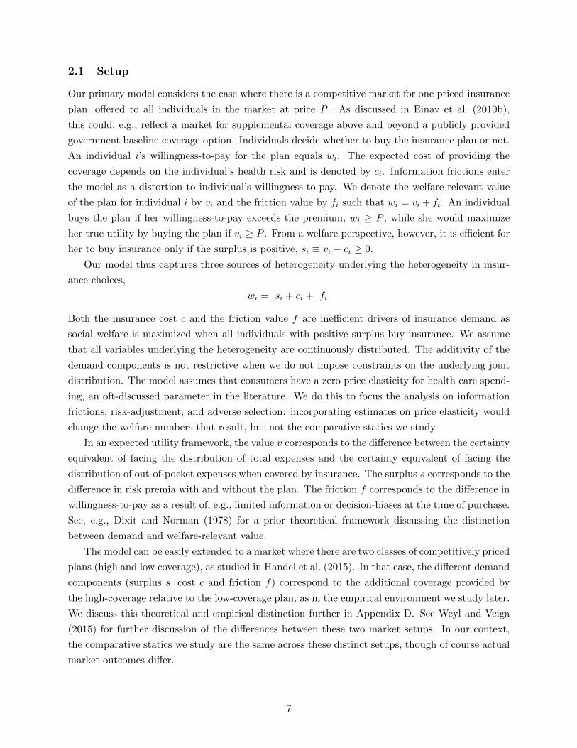
In an adversely selected market, individuals who are more costly to insure have a higher willing-

ness to buy insurance. This causes the marginal cost curve to be downward sloping, as illustrated

in Figure 1. The average cost curve lies above the marginal cost curve and is downward-sloping

as well. Conversely, in an advantageously selected market, the cost curves would be upward slop-

ing and the marginal cost cost curve would lie above the average cost curve. The competitive

equilibrium is simply given by the intersection of the demand curve and the average cost curve.

To evaluate welfare we need the value of insurance relative to its cost and thus compare the

value curve (rather than the demand curve) to the marginal cost curve. Information frictions drive

a wedge between the demand curve and the value curve in two ways. For a uniform friction fi = f ,

the value curve is parallel to the demand curve, EP (v) = P − f . If the friction value is positive,

individuals tend to overestimate the insurance value and the value curve is a downward shift of

the demand curve. This is the case when all individuals overestimate the expected expenses or the

coverage that is provided in the same way. Second, heterogeneous demand frictions fi = f+εi cause

the value curve to be a counter-clockwise rotation of the demand curve when the friction variation is

independent. Individuals with higher willingness-to-pay tend to overestimate the value of insurance

14While equilibrium price and coverage are different under imperfect competition, the sorting of individuals remainsthe same. Hence, conditional on the change in equilibrium coverage, the welfare evaluation of policy interventionsremains the same in other market environments.

9

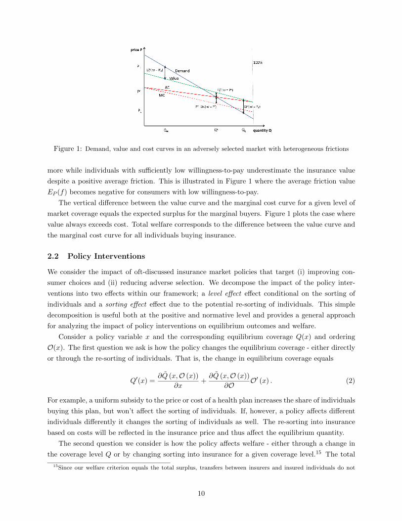
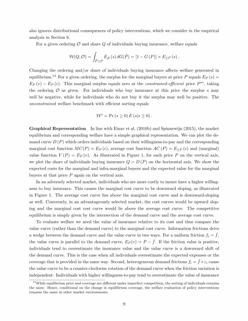
Figure 1: Demand, value and cost curves in an adversely selected market with heterogeneous frictions

more while individuals with sufficiently low willingness-to-pay underestimate the insurance value

despite a positive average friction. This is illustrated in Figure 1 where the average friction value

EP (f) becomes negative for consumers with low willingness-to-pay.

The vertical difference between the value curve and the marginal cost curve for a given level of

market coverage equals the expected surplus for the marginal buyers. Figure 1 plots the case where

value always exceeds cost. Total welfare corresponds to the difference between the value curve and

the marginal cost curve for all individuals buying insurance.

2.2 Policy Interventions

We consider the impact of oft-discussed insurance market policies that target (i) improving con-

sumer choices and (ii) reducing adverse selection. We decompose the impact of the policy inter-

ventions into two effects within our framework; a level effect effect conditional on the sorting of

individuals and a sorting effect effect due to the potential re-sorting of individuals. This simple

decomposition is useful both at the positive and normative level and provides a general approach

for analyzing the impact of policy interventions on equilibrium outcomes and welfare.

Consider a policy variable x and the corresponding equilibrium coverage Q(x) and ordering

O(x). The first question we ask is how the policy changes the equilibrium coverage - either directly

or through the re-sorting of individuals. That is, the change in equilibrium coverage equals

Q′(x) =∂Q (x,O (x))

∂x+∂Q (x,O (x))

∂OO′ (x) . (2)

For example, a uniform subsidy to the price or cost of a health plan increases the share of individuals

buying this plan, but won’t affect the sorting of individuals. If, however, a policy affects different

individuals differently it changes the sorting of individuals as well. The re-sorting into insurance

based on costs will be reflected in the insurance price and thus affect the equilibrium quantity.

The second question we consider is how the policy affects welfare - either through a change in

the coverage level Q or by changing sorting into insurance for a given coverage level.15 The total

15Since our welfare criterion equals the total surplus, transfers between insurers and insured individuals do not

10

welfare impact of a budget-balanced change in the policy equals

W ′ (x) =∂W (Q (x) ,O (x))

∂QQ′ (x) +

∂W (Q (x) ,O (x))

∂OO′ (x) . (3)

The welfare impact of changing the level of coverage simply depends on whether the policy inter-

vention brings the equilibrium coverage closer to the efficient coverage. If the expected surplus for

the marginal buyers is positive, individuals tend to be under-insured and the equilibrium price is

inefficiently high. This underlies the analysis of price subsidies and mandates in adversely selected

markets in Einav et al. (2010b) and Hackmann et al. (2015). However, these studies only considered

the pricing inefficiency coming from the supply side. The presence of demand frictions may worsen

the supply side inefficiency, but can also reduce this inefficiency and potentially reverse the welfare

impact of an increase in equilibrium coverage, as shown in Spinnewijn (2015). The interaction

between supply and demand frictions is illustrated clearly by decomposing the marginal surplus at

the equilibrium price P (x) as

EP (x) (s) = EP (x) (w − c− f) = [P (x)− EP (x) (c)]− EP (x) (f) . (4)

From the supply side, insurance companies charge prices that are different from the marginal cost in

selection markets, P (x) 6= EP (x) (c). In a competitive market, the wedge between the average cost

and marginal cost of providing insurance causes under-insurance in an adversely selected market,

but over-insurance in an advantageously selected market. From the demand side, frictions cause

individuals to buy coverage even if their valuation is below the price and vice versa. In particular,

if the marginal buyers overestimate the insurance value (EP (f) > 0), this tends to make the

equilibrium coverage inefficiently high. The opposite is true if the marginal buyers underestimate

the insurance value (EP (f) < 0). The specific welfare impact of different scenarios depends on

these offsetting effects, and which dominates.

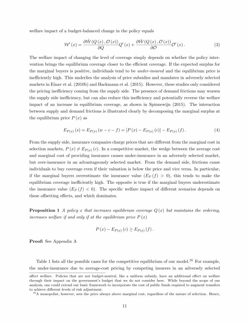
Proposition 1 A policy x that increases equilibrium coverage Q (x) but maintains the ordering,

increases welfare if and only if at the equilibrium price P (x)

P (x)− EP (x) (c) ≥ EP (x) (f) .

Proof: See Appendix A

Table 1 lists all the possible cases for the competitive equilibrium of our model.16 For example,

the under-insurance due to average-cost pricing by competing insurers in an adversely selected

affect welfare. Policies that are not budget-neutral, like a uniform subsidy, have an additional effect on welfarethrough their impact on the government’s budget that we do not consider here. While beyond the scope of ouranalysis, one could extend our basic framework to incorporate the cost of public funds required to augment transfersto achieve different levels of risk adjustment.

16A monopolist, however, sets the price always above marginal cost, regardless of the nature of selection. Hence,

11

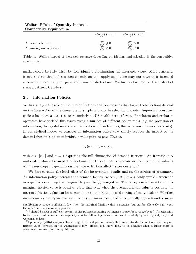
Welfare Effect of Quantity IncreaseCompetitive Equilibrium

EP (x) (f) > 0 EP (x) (f) < 0

Adverse selection ∂W∂Q ≷ 0 ∂W

∂Q > 0

Advantageous selection ∂W∂Q < 0 ∂W

∂Q ≷ 0

Table 1: Welfare impact of increased coverage depending on frictions and selection in the competitive

equilibrium

market could be fully offset by individuals overestimating the insurance value. More generally,

it makes clear that policies focused only on the supply side alone may not have their intended

effects after accounting for potential demand side frictions. We turn to this later in the context of

risk-adjustment transfers.

2.3 Information Policies

We first analyze the role of information frictions and how policies that target these frictions depend

on the interaction of the demand and supply frictions in selection markets. Improving consumer

choices has been a major concern underlying US health care reforms. Regulators and exchange

operators have tackled this issues using a number of different policy tools (e.g the provision of

information, the regulation and standardization of plan features, the reduction of transaction costs).

In our stylized model we consider an information policy that simply reduces the impact of the

demand friction f on an individual’s willingness to pay. That is,

wi (α) = wi − α× fi

with α ∈ [0, 1] and α = 1 capturing the full elimination of demand frictions. An increase in α

uniformly reduces the impact of frictions, but this can either increase or decrease an individual’s

willingness-to-pay depending on the type of friction affecting her demand.17

We first consider the level effect of the intervention, conditional on the sorting of consumers.

An information policy increases the demand for insurance - just like a subsidy would - when the

average friction among the marginal buyers EP (f) is negative. The policy works like a tax if this

marginal friction value is positive. Note that even when the average friction value is positive, the

marginal friction value can be negative due to the friction-based sorting of individuals.18 Whether

an information policy increases or decreases insurance demand thus crucially depends on the mean

equilibrium coverage is efficiently low when the marginal friction value is negative, but can be efficiently high whenthe marginal friction value is positive.

17f should be seen as sufficient for any choice policies impacting willingness-to-pay for coverage by αfi. An extensionto the model could consider heterogeneity in α for different policies as well as the underlying heterogeneity in f thatwe consider here.

18Spinnewijn (2015) analyzes this sorting effect in depth and shows that under standard conditions the marginalfriction value increases in the willingness-to-pay. Hence, it is more likely to be negative when a larger share ofconsumers buy insurance in equilibrium.

12

and variance of the frictions (in addition to the other primitives affecting the marginal consumers).

Any policy intervention that induces more individuals at the margin to buy insurance decreases

the equilibrium price in an adversely selected market (since average cost exceeds marginal cost).

This further increases equilibrium coverage. In a competitive equilibrium, the impact of a simple

subsidy on the equilibrium quantity is shown to be

ηc ≡ g (P c)

1− [E≥P c (c)− EP c(c)] |εD(P c)|P c

and is thus larger in a market that is more adversely selected. Conditional on the ordering of

individuals, an information policy simply scales the impact of a subsidy depending on the sign and

size of the marginal friction value,

∂Q (α,O (α))

∂α= −EP c (f)× ηc.

For a uniform friction, this level effect would be the only impact on the market equilibrium.

The welfare implication then depends on whether the insurance surplus among the marginal buyers

EP c (s) is positive or negative, in line with Proposition 1.19

With heterogeneous frictions, an information policy also changes the ordering of individuals’

willingness-to-pay. In particular, the policy reduces the willingness for individuals with positive

friction values to buy insurance and vice versa. Among the marginal buyers those with large friction

values will have lower true values, while those with low friction values will have higher true values.

Hence, a simple selection effect is underlying the re-sorting of individuals; an information policy

encourages individuals with high true value to buy more insurance and discourages individuals with

low true value from more buying insurance. The policy thus necessarily increases the expected true

value E≥P (v) for a given share of buyers. This sorting effect depends on the covariance between

true value and friction value among the marginal buyers,

covP (v, f) = covP (P − (1− α) f, f) = − (1− α) varP (f) ≤ 0,

and is indeed always negative. The larger the variance in frictions, the more a friction-reducing

policy increases the sorting based on true value. Figure 2 illustrates this sorting effect showing

the combinations of true values v and friction values f for which an individual buys insurance. A

downward sloping curve implied by v + (1− α) f = P separates the groups who buy the different

plans. This curve flattens due to an information policy; individuals with high true value become

more likely to buy insurance, while individuals with low true value value become less likely to buy

insurance. Both changes increases the expected true value E≥P (v).

As the insurance value depends on both cost and surplus, decomposing the sorting effect for

costs and surplus is key. The re-sorting based on costs determines the impact on the equilibrium

19If the information friction more than offsets the supply friction, |EP (f)| ≥ |P − EP (c)|, the welfare gain of aninformation policy may be initially positive (i.e., for α = 0), but becomes negative eventually when α converges to 1such that (1− α)

∣∣EP (α) (f)∣∣ < ∣∣P (α)− EP (α) (c)

∣∣.13

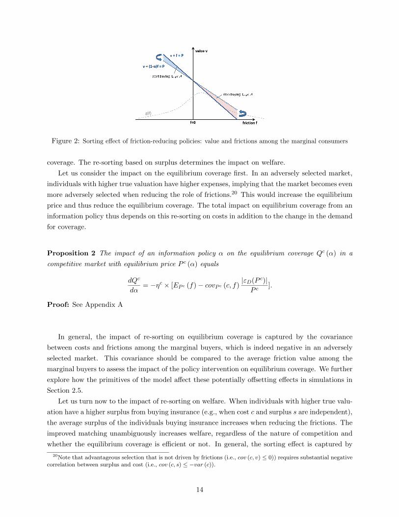
Figure 2: Sorting effect of friction-reducing policies: value and frictions among the marginal consumers

coverage. The re-sorting based on surplus determines the impact on welfare.

Let us consider the impact on the equilibrium coverage first. In an adversely selected market,

individuals with higher true valuation have higher expenses, implying that the market becomes even

more adversely selected when reducing the role of frictions.20 This would increase the equilibrium

price and thus reduce the equilibrium coverage. The total impact on equilibrium coverage from an

information policy thus depends on this re-sorting on costs in addition to the change in the demand

for coverage.

Proposition 2 The impact of an information policy α on the equilibrium coverage Qc (α) in a

competitive market with equilibrium price P c (α) equals

dQc

dα= −ηc × [EP c (f)− covP c (c, f)

|εD(P c)|P c

].


In general, the impact of re-sorting on equilibrium coverage is captured by the covariance

between costs and frictions among the marginal buyers, which is indeed negative in an adversely

selected market. This covariance should be compared to the average friction value among the

marginal buyers to assess the impact of the policy intervention on equilibrium coverage. We further

explore how the primitives of the model affect these potentially offsetting effects in simulations in

Section 2.5.

Let us turn now to the impact of re-sorting on welfare. When individuals with higher true valu-

ation have a higher surplus from buying insurance (e.g., when cost c and surplus s are independent),

the average surplus of the individuals buying insurance increases when reducing the frictions. The

improved matching unambiguously increases welfare, regardless of the nature of competition and

whether the equilibrium coverage is efficient or not. In general, the sorting effect is captured by

20Note that advantageous selection that is not driven by frictions (i.e., cov (c, v) ≤ 0)) requires substantial negativecorrelation between surplus and cost (i.e., cov (c, s) ≤ −var (c)).

14

the covariance between the friction value and the surplus among the marginal buyers. The total

welfare change then depends on this sorting effect in addition to the welfare impact from the change

in coverage.

Proposition 3 The impact of an information policy on equilibrium welfare equals

dWdα

= EP (α) (s)Q′ (α)− covP (α) (s, f) gw(α) (P (α)) .


To evaluate the sorting effect on welfare the comparison between the relative contributions of

re-sorting based on cost compared to re-sorting based on surplus induced by the information policy

becomes key. Propositions 2 and 3 indicate that at the margin these effects are captured by the

conditional covariance covP (c, f) and covP (s, f) respectively. These effects need to be compared

to the level change in insurance demand captured by the mean friction value among the marginal

buyers EP c (f).

Corollary 1 In a competitive equilibrium with under-insurance, EP c (s) > 0, the welfare gain

from reducing information frictions increases in −covP c (s, f), but decreases in −covP c (c, f) and

in EP c (f).

Proof: From Propositions 2 and 3, we can simply re-write the impact on welfare in a competitive

equilibrium as

W ′ (α) = −EP c (s) ηc[EP c (f)− covP c (c, f)|εD(P c)|P c

]− covP c (s, f) gw(α) (P c)

= −EP c (f) ηcEP c (s) + covP c (c, f)|εD(P c)|P c

ηcEP c (s)− covP c (s, f) gw(α) (P c)

The impact of covP c(c, f) is unambiguously positive in a market with under-insurance, EP c (s) ≥0.

It is clear that due to the re-sorting of consumers, friction-reducing policies change the demand,

value and cost curves and these changes depend on the underlying micro-foundations. The original

demand, value and cost curves do not provide sufficient information for analyzing the market

and welfare impact of such policies. However, the simple formulas in the Propositions (exploiting

marginal policy changes) clearly indicate the key statistics underlying the overall effects we should

anticipate. One important observation is that we can rewrite the conditional covariances (as used

in the Propositions) in terms of conditional variances of the demand primitives:

covw(c, f) =1

2[varw(s)− varw(c)− varw(f)]

covw(s, f) =1

2[varw(c)− varw(s)− varw(f)].

15

This shows that the relative variance in cost and surplus underlying the demand for insurance is

first-order. The higher the variance in costs relative to surplus the more likely that the increase in

adverse selection dominates the increased selection on surplus in response to an information policy.

This insight in our framework with consumer frictions builds on related insights in Veiga and Weyl

(2015) studying equilibrium in selection markets.

The (unconditional) correlations between the different demand components matter as well be-

cause they affect the variances conditional on the willingness to pay. First, positive correlation

between two demand components increases the conditional covariance between these two compo-

nents. For example, positive correlation between frictions and costs will reduce the variance in

costs and frictions conditional on the willingness-to-pay.21 Second, negative correlation with a

third demand component increases the conditional covariance between the first two components.

For example, if individuals with higher cost have low insurance value, like in an advantageously

selected market, the conditional covariance between cost and friction will be positive.

2.4 Risk-adjustment Transfers

The impact of demand frictions on equilibrium and welfare indicates their relevance for the eval-

uation of policies that target supply side frictions. We explore the importance of this interaction

for cost subsidies and risk-adjustment transfers in particular. These policies are key features of US

health reform, e.g. in the state exchanges set up under the ACA, as well as many other efforts to

mitigate adverse selection and expand insurance coverage.

Risk-adjustment transfers subsidize the cost of providing insurance for an insurer based on the

underlying risk of the insured individual. In practice, risk adjustment is implemented as a policy

that facilitates transfers based on the realized or expected cost of the insured pool for each insurer.22

Introducing risk-adjustment in our stylized model, the expected cost to the insurer of providing

insurance to individual i becomes

ci (β) = ci − β × [ci − Ec]

with β ∈ [0, 1] and β = 1 capturing full risk-adjustment. An increase in β makes the expected

cost of providing insurance less dependent on the individual’s risk type, but does not affect the

ordering of individuals directly.23 In an adversely selected market, the average cost among the infra-

marginal individuals unambiguously decreases for a given price. Hence, risk-adjustment transfers

unambiguously reduce the equilibrium price and increases equilibrium coverage in a competitive

21For example, in the extreme case with c = f , we have covP (c, f) = varP (c) = varP (f) ≥ 0.22Whether risk adjustment compensates plans based on realized versus expected cost is an important question for

the efficiency of incentives to insurers that trade off selection incentives against the power of cost reduction incentivesconditional on enrollment. Geruso and McGuire (2014) study the issue in detail and we abstract from this tradeoffin our model and empirical implementation.

23This contrast with risk-rating where high-risk individuals pay a higher insurance premium than low-risk individ-uals. The analysis of the sorting effect of such policy is analogue to our analysis of information policies. Reducingthe impact of costs will reduce selection based on risks, but increase selection based on frictions and on surplus.

16

market. That is,

Q′ (β) = ηc × [E≥P (c)− Ec],

where ηc is the equilibrium response to a uniform subsidy.24 The more adversely selected the market

is, the larger the impact of risk-adjustment transfers on equilibrium coverage. This indicates a first

key interaction with information frictions as they can reduce selection on costs. Risk-adjustment

transfers will affect the equilibrium by more the less plan selection is affected by demand frictions.

Since risk-adjustment transfers preserve the ordering of individuals’ willingness-to-pay, the pol-

icy affects welfare only through the change in equilibrium coverage. The impact on welfare thus

depends on the surplus among the marginal buyers in line with Proposition 1. This indicates a sec-

ond key interaction with information frictions as the demand and supply frictions jointly determine

whether the market is under- or over-insured. In an adversely selected market where information

frictions reduce under-insurance, the presence of these frictions not only reduces the effectiveness

of risk-adjustment transfers in increasing coverage, but also reduces the welfare gain from that

increase. The following Proposition summarizes the potential effects.

Proposition 4 A risk-adjustment policy β increases equilibrium coverage in a competitive market

by

Q′ (β) = ηc × [E≥P (c)− Ec].

The impact on welfare equals

W ′ (β) = EP (β) (s)Q′ (β) .


Graphically, risk-adjustment transfers will flatten the cost curves relevant to the insurer relative

to the demand curve. The value curve and marginal cost curve relevant for evaluating welfare are

unaffected since the policy does not affect the ordering.25

We note that our risk adjustment framework assumes that a regulatory budget exists to fund

risk adjustment transfers, and our welfare analysis does not explicitly consider the budgetary cost

of the risk-adjustment policy equal to β × [E≥P c (c)− Ec]×Q (β). Though we do not do so here,

it is not difficult to extend the model to account for different costs of funding.

This analysis highlights the important interaction between demand and supply side policies.

Information policies can increase the effectiveness of risk-adjustment transfers and increase their

impact on welfare. By the same token, the negative consequences of information policies through

the increased adverse selection could be directly addressed through risk-adjustment transfers or any

24Note that in an adversely selected market risk-adjustment transfers can never decrease the equilibrium pricepc below the average cost E[c] for β ∈ [0, 1]. Hence, in contrast with a standard subsidy, it may be impossible todecentralize the (constrained) efficient allocation.

25Note that the key difference between the uniform subsidy and the risk-adjustment transfers is that in the caseof a subsidy the equilibrium is determined by a vertical shift of the original cost curves, while in the case of risk-adjustment transfers the equilibrium is determined by the original cost curves net of the risk-adjustment transfersimplying rotations as discussed before.

17

other policy that mitigates the increase in the equilibrium price. We confirm the complementarity

between information policies and risk-adjustment in the simulations below.

2.5 Simulations

To provide further insights on how the different model components impact positive and normative

outcomes under different policies, we present a series of simulations. We use these simulations to il-

lustrate the role that the key micro-foundations described in this section play in determining market

outcomes under (i) no policy interventions (ii) friction-reducing policies and (iii) risk-adjustment

policies. Specifically, we distinguish between cases where friction-reducing interventions have pos-

itive vs. negative welfare impacts, and cases where effective risk-adjustment policies are essential

prior to implementing friction-reducing policies.

Our focus is on a market setup in the mold of Einav et al. (2010b), similar to our primary model,

where insurers compete to offer supplemental insurance relative to a baseline publicly provided plan.

See Appendix D for similar simulations on markets with two competitively priced plans, as studied

in Handel et al. (2015).

The baseline plan for these simulations has a deductible of $3,000, with 10% coinsurance after

that point, up to an out-of-pocket maximum of $7, 000 (this plan has a 66% actuarial value for

our baseline costs below). The supplemental coverage that insurers compete to offer covers all

out-of-pocket spending in the baseline plan, and thus brings all consumers up to full insurance.

These plans are similar to the minimum and maximum coverage levels regulated in the state-based

exchanges set up in the ACA, and also mimic the plans we study in our empirical environment later

in this paper. Importantly, in our environment with risk averse consumers and no moral hazard,

all consumers purchase full insurance in the first-best. In each simulation we simulate the market

for 10,000 consumers.

We study a range of scenarios that vary in terms of the underlying means and variances of

(i) consumer surplus from risk protection (ii) consumer costs and (iii) consumer choice frictions.

Table 2 describes the underlying distributions for the different cases we study. We simulate two

scenarios for consumer yearly expected costs: both have the same mean of just above $5,000. The

first scenario has a high standard deviation of expected costs in the population of $6,819 while

the second has a low standard deviation of $2,990. Each scenario is generated from an underlying

lognormal distribution. The within-year standard deviation in costs for a family is 3,000 plus 1.2

times their yearly expected costs in both scenarios. The impact of frictions on demand for generous

insurance is generated from a normal distribution. The high (low) mean is a $2,500 ($0) shift in

willingness-to-pay while the high (low) standard deviation we study is $2,000 ($500). We study all

four combinations of these high/low means and variances. Finally, for consumer risk aversion, we

also study four combinations from normal distributions with high/low means and variances. The

high (low) CARA mean is 1 ∗ 10−3 (4 ∗ 10−4) while the high (low) standard deviation is 4 ∗ 10−4

(1 ∗ 10−4), with values truncated above 0. The left panel in Figure 3 shows the two distributions

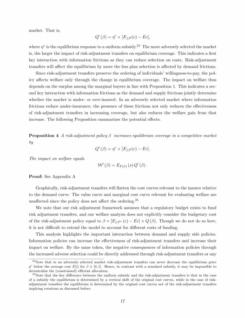
of costs studied. The right panel in Figure 3 shows the distribution of surplus in the market when

18

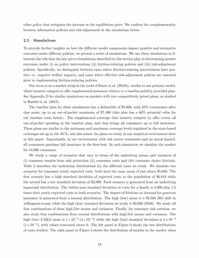
SimulationsKey Micro-Foundations

Total Costs - µc* 5,373Total Costs - σc - High* 6,819Total Costs - σc - Low* 2,990

Frictions - µf - High** 2,500Frictions - µf - Low** 0Frictions - σf - High** 2,000Frictions - σf - Low** 500

Risk Aversion - µs - High*** 1 ∗ 10−3

Risk Aversion - µs - Low*** 3 ∗ 10−4

Risk Aversion - σs - High*** 4 ∗ 10−4

Risk Aversion - σs - Low*** 1 ∗ 10−4

*Costs simulated from lognormal distribution.**Frictions Simulated from normal distribution.***Risk preferences simulated from normal distribution, truncated above 0.

Table 2: This table presents the underlying distributions of micro-foundations for the differentsimulation scenarios we study.

Figure 3: The left panel shows the two different cost distributions used in our simulations. The right panelshows the resulting surplus distributions under the different scenarios for risk protection, conditional on thecost distribution with high variance.

the variance in costs is high under the cases of (i) high mean and variance of risk aversion (ii) low

mean and high variance of risk aversion and (iii) low mean and low variance of risk aversion.

We first present a specific simulation example to illustrate the very different impact frictions can

have on equilibrium and welfare depending on the primitives of the model. We then systematically

investigate positive and normative patterns across a wider range of simulations. Our example

focuses on two markets with a high variance of costs and surplus, and a low mean, but high

variance of frictions. The two markets differ only in terms of mean surplus: one has low mean

19

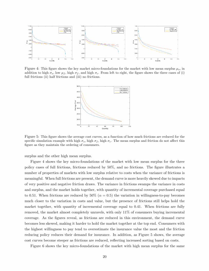
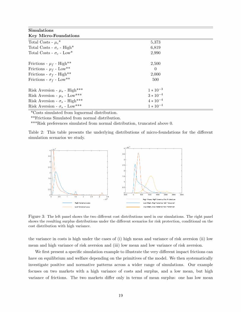
Figure 4: This figure shows the key market micro-foundations for the market with low mean surplus µs, inaddition to high σs, low µf , high σf , and high σc. From left to right, the figure shows the three cases of (i)full frictions (ii) half frictions and (iii) no frictions.

Figure 5: This figure shows the average cost curves, as a function of how much frictions are reduced for thespecific simulation example with high σs, high σf , high σc. The mean surplus and friction do not affect thisfigure as they maintain the ordering of consumers.

surplus and the other high mean surplus.

Figure 4 shows the key micro-foundations of the market with low mean surplus for the three

policy cases of full frictions, frictions reduced by 50%, and no frictions. The figure illustrates a

number of properties of markets with low surplus relative to costs when the variance of frictions is

meaningful. When full frictions are present, the demand curve is more heavily skewed due to impacts

of very positive and negative friction draws. The variance in frictions swamps the variance in costs

and surplus, and the market holds together, with quantity of incremental coverage purchased equal

to 0.51. When frictions are reduced by 50% (α = 0.5) the variation in willingness-to-pay becomes

much closer to the variation in costs and value, but the presence of frictions still helps hold the

market together, with quantity of incremental coverage equal to 0.41. When frictions are fully

removed, the market almost completely unravels, with only 11% of consumers buying incremental

coverage. As the figures reveal, as frictions are reduced in this environment, the demand curve

becomes less skewed, making it harder to hold the market together at the top end. Consumers with

the highest willingness to pay tend to overestimate the insurance value the most and the friction

reducing policy reduces their demand for insurance. In addition, as Figure 5 shows, the average

cost curves become steeper as frictions are reduced, reflecting increased sorting based on costs.

Figure 6 shows the key micro-foundations of the market with high mean surplus for the same

20

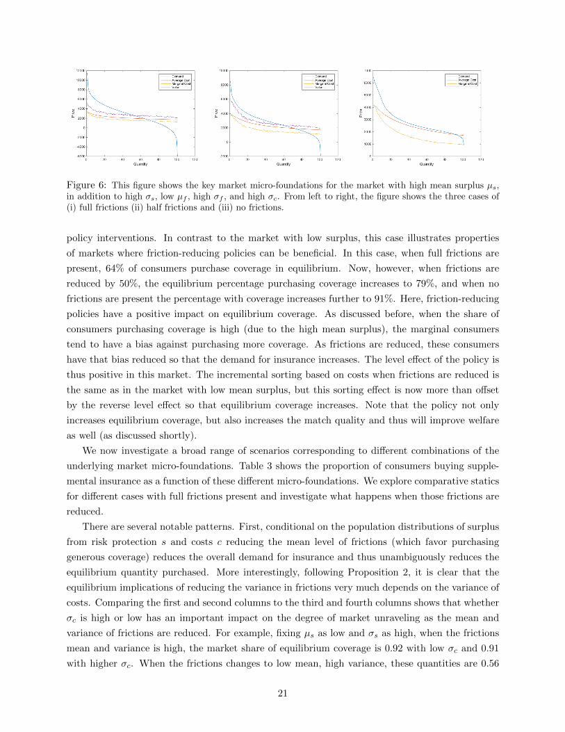
Figure 6: This figure shows the key market micro-foundations for the market with high mean surplus µs,in addition to high σs, low µf , high σf , and high σc. From left to right, the figure shows the three cases of(i) full frictions (ii) half frictions and (iii) no frictions.

policy interventions. In contrast to the market with low surplus, this case illustrates properties

of markets where friction-reducing policies can be beneficial. In this case, when full frictions are

present, 64% of consumers purchase coverage in equilibrium. Now, however, when frictions are

reduced by 50%, the equilibrium percentage purchasing coverage increases to 79%, and when no

frictions are present the percentage with coverage increases further to 91%. Here, friction-reducing

policies have a positive impact on equilibrium coverage. As discussed before, when the share of

consumers purchasing coverage is high (due to the high mean surplus), the marginal consumers

tend to have a bias against purchasing more coverage. As frictions are reduced, these consumers

have that bias reduced so that the demand for insurance increases. The level effect of the policy is

thus positive in this market. The incremental sorting based on costs when frictions are reduced is

the same as in the market with low mean surplus, but this sorting effect is now more than offset

by the reverse level effect so that equilibrium coverage increases. Note that the policy not only

increases equilibrium coverage, but also increases the match quality and thus will improve welfare

as well (as discussed shortly).

We now investigate a broad range of scenarios corresponding to different combinations of the

underlying market micro-foundations. Table 3 shows the proportion of consumers buying supple-

mental insurance as a function of these different micro-foundations. We explore comparative statics

for different cases with full frictions present and investigate what happens when those frictions are

reduced.

There are several notable patterns. First, conditional on the population distributions of surplus

from risk protection s and costs c reducing the mean level of frictions (which favor purchasing

generous coverage) reduces the overall demand for insurance and thus unambiguously reduces the

equilibrium quantity purchased. More interestingly, following Proposition 2, it is clear that the

equilibrium implications of reducing the variance in frictions very much depends on the variance of

costs. Comparing the first and second columns to the third and fourth columns shows that whether

σc is high or low has an important impact on the degree of market unraveling as the mean and

variance of frictions are reduced. For example, fixing µs as low and σs as high, when the frictions

mean and variance is high, the market share of equilibrium coverage is 0.92 with low σc and 0.91

with higher σc. When the frictions changes to low mean, high variance, these quantities are 0.56

21

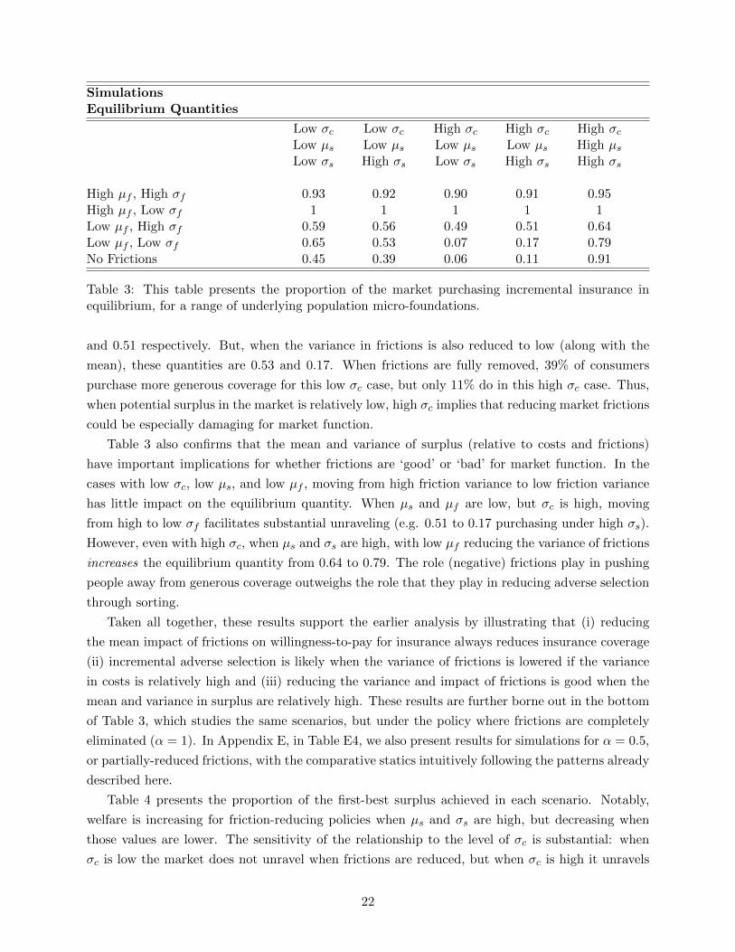
SimulationsEquilibrium Quantities

Low σc Low σc High σc High σc High σcLow µs Low µs Low µs Low µs High µsLow σs High σs Low σs High σs High σs

High µf , High σf 0.93 0.92 0.90 0.91 0.95High µf , Low σf 1 1 1 1 1Low µf , High σf 0.59 0.56 0.49 0.51 0.64Low µf , Low σf 0.65 0.53 0.07 0.17 0.79No Frictions 0.45 0.39 0.06 0.11 0.91

Table 3: This table presents the proportion of the market purchasing incremental insurance inequilibrium, for a range of underlying population micro-foundations.

and 0.51 respectively. But, when the variance in frictions is also reduced to low (along with the

mean), these quantities are 0.53 and 0.17. When frictions are fully removed, 39% of consumers

purchase more generous coverage for this low σc case, but only 11% do in this high σc case. Thus,

when potential surplus in the market is relatively low, high σc implies that reducing market frictions

could be especially damaging for market function.

Table 3 also confirms that the mean and variance of surplus (relative to costs and frictions)

have important implications for whether frictions are ‘good’ or ‘bad’ for market function. In the

cases with low σc, low µs, and low µf , moving from high friction variance to low friction variance

has little impact on the equilibrium quantity. When µs and µf are low, but σc is high, moving

from high to low σf facilitates substantial unraveling (e.g. 0.51 to 0.17 purchasing under high σs).

However, even with high σc, when µs and σs are high, with low µf reducing the variance of frictions

increases the equilibrium quantity from 0.64 to 0.79. The role (negative) frictions play in pushing

people away from generous coverage outweighs the role that they play in reducing adverse selection

through sorting.

Taken all together, these results support the earlier analysis by illustrating that (i) reducing

the mean impact of frictions on willingness-to-pay for insurance always reduces insurance coverage

(ii) incremental adverse selection is likely when the variance of frictions is lowered if the variance

in costs is relatively high and (iii) reducing the variance and impact of frictions is good when the

mean and variance in surplus are relatively high. These results are further borne out in the bottom

of Table 3, which studies the same scenarios, but under the policy where frictions are completely

eliminated (α = 1). In Appendix E, in Table E4, we also present results for simulations for α = 0.5,

or partially-reduced frictions, with the comparative statics intuitively following the patterns already

described here.

Table 4 presents the proportion of the first-best surplus achieved in each scenario. Notably,

welfare is increasing for friction-reducing policies when µs and σs are high, but decreasing when

those values are lower. The sensitivity of the relationship to the level of σc is substantial: when

σc is low the market does not unravel when frictions are reduced, but when σc is high it unravels

22

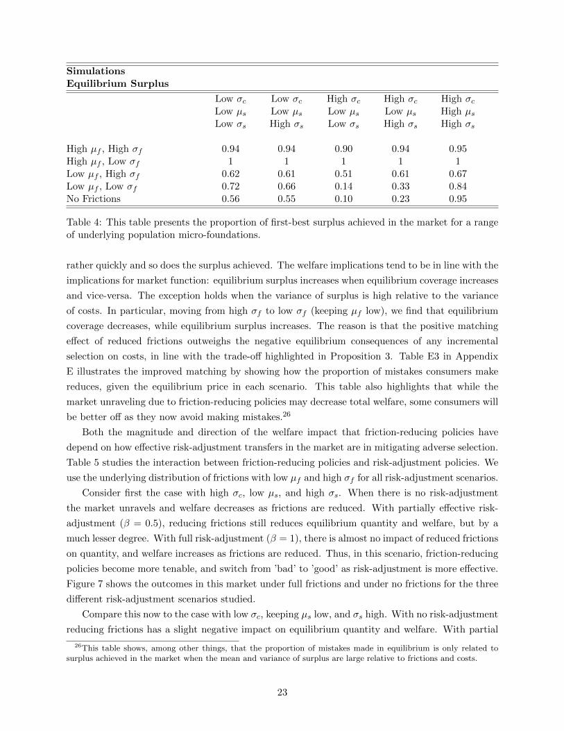
SimulationsEquilibrium Surplus



Table 4: This table presents the proportion of first-best surplus achieved in the market for a rangeof underlying population micro-foundations.

rather quickly and so does the surplus achieved. The welfare implications tend to be in line with the

implications for market function: equilibrium surplus increases when equilibrium coverage increases

and vice-versa. The exception holds when the variance of surplus is high relative to the variance

of costs. In particular, moving from high σf to low σf (keeping µf low), we find that equilibrium

coverage decreases, while equilibrium surplus increases. The reason is that the positive matching

effect of reduced frictions outweighs the negative equilibrium consequences of any incremental

selection on costs, in line with the trade-off highlighted in Proposition 3. Table E3 in Appendix

E illustrates the improved matching by showing how the proportion of mistakes consumers make

reduces, given the equilibrium price in each scenario. This table also highlights that while the

market unraveling due to friction-reducing policies may decrease total welfare, some consumers will

be better off as they now avoid making mistakes.26

Both the magnitude and direction of the welfare impact that friction-reducing policies have

depend on how effective risk-adjustment transfers in the market are in mitigating adverse selection.

Table 5 studies the interaction between friction-reducing policies and risk-adjustment policies. We

use the underlying distribution of frictions with low µf and high σf for all risk-adjustment scenarios.

Consider first the case with high σc, low µs, and high σs. When there is no risk-adjustment

the market unravels and welfare decreases as frictions are reduced. With partially effective risk-

adjustment (β = 0.5), reducing frictions still reduces equilibrium quantity and welfare, but by a

much lesser degree. With full risk-adjustment (β = 1), there is almost no impact of reduced frictions

on quantity, and welfare increases as frictions are reduced. Thus, in this scenario, friction-reducing

policies become more tenable, and switch from ’bad’ to ’good’ as risk-adjustment is more effective.

Figure 7 shows the outcomes in this market under full frictions and under no frictions for the three

different risk-adjustment scenarios studied.

Compare this now to the case with low σc, keeping µs low, and σs high. With no risk-adjustment

reducing frictions has a slight negative impact on equilibrium quantity and welfare. With partial

26This table shows, among other things, that the proportion of mistakes made in equilibrium is only related tosurplus achieved in the market when the mean and variance of surplus are large relative to frictions and costs.

23

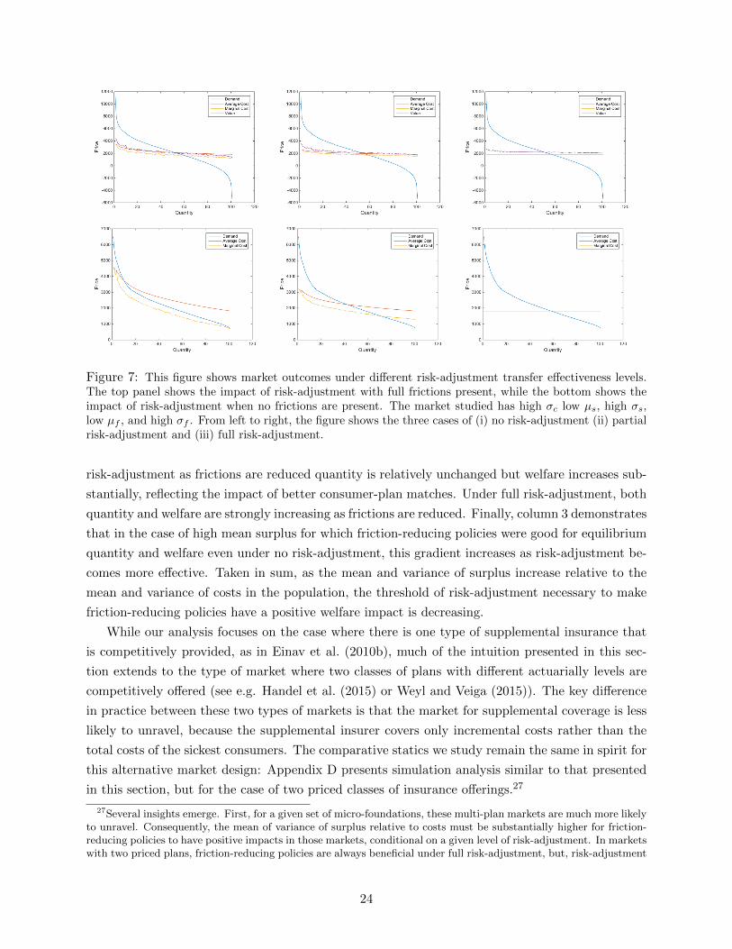
Figure 7: This figure shows market outcomes under different risk-adjustment transfer effectiveness levels.The top panel shows the impact of risk-adjustment with full frictions present, while the bottom shows theimpact of risk-adjustment when no frictions are present. The market studied has high σc low µs, high σs,low µf , and high σf . From left to right, the figure shows the three cases of (i) no risk-adjustment (ii) partialrisk-adjustment and (iii) full risk-adjustment.

risk-adjustment as frictions are reduced quantity is relatively unchanged but welfare increases sub-

stantially, reflecting the impact of better consumer-plan matches. Under full risk-adjustment, both

quantity and welfare are strongly increasing as frictions are reduced. Finally, column 3 demonstrates

that in the case of high mean surplus for which friction-reducing policies were good for equilibrium

quantity and welfare even under no risk-adjustment, this gradient increases as risk-adjustment be-

comes more effective. Taken in sum, as the mean and variance of surplus increase relative to the

mean and variance of costs in the population, the threshold of risk-adjustment necessary to make

friction-reducing policies have a positive welfare impact is decreasing.

While our analysis focuses on the case where there is one type of supplemental insurance that

is competitively provided, as in Einav et al. (2010b), much of the intuition presented in this sec-

tion extends to the type of market where two classes of plans with different actuarially levels are

competitively offered (see e.g. Handel et al. (2015) or Weyl and Veiga (2015)). The key difference

in practice between these two types of markets is that the market for supplemental coverage is less

likely to unravel, because the supplemental insurer covers only incremental costs rather than the

total costs of the sickest consumers. The comparative statics we study remain the same in spirit for

this alternative market design: Appendix D presents simulation analysis similar to that presented

in this section, but for the case of two priced classes of insurance offerings.27

27Several insights emerge. First, for a given set of micro-foundations, these multi-plan markets are much more likelyto unravel. Consequently, the mean of variance of surplus relative to costs must be substantially higher for friction-reducing policies to have positive impacts in those markets, conditional on a given level of risk-adjustment. In marketswith two priced plans, friction-reducing policies are always beneficial under full risk-adjustment, but, risk-adjustment

24

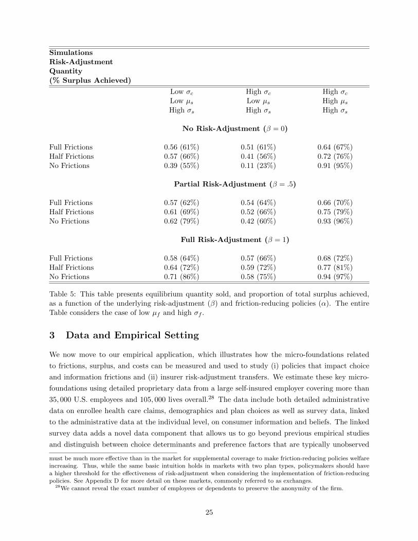
SimulationsRisk-AdjustmentQuantity(% Surplus Achieved)

Low σc High σc High σcLow µs Low µs High µsHigh σs High σs High σs

No Risk-Adjustment (β = 0)

Full Frictions 0.56 (61%) 0.51 (61%) 0.64 (67%)Half Frictions 0.57 (66%) 0.41 (56%) 0.72 (76%)No Frictions 0.39 (55%) 0.11 (23%) 0.91 (95%)

Partial Risk-Adjustment (β = .5)


Full Risk-Adjustment (β = 1)


Table 5: This table presents equilibrium quantity sold, and proportion of total surplus achieved,as a function of the underlying risk-adjustment (β) and friction-reducing policies (α). The entireTable considers the case of low µf and high σf .

3 Data and Empirical Setting

We now move to our empirical application, which illustrates how the micro-foundations related

to frictions, surplus, and costs can be measured and used to study (i) policies that impact choice

and information frictions and (ii) insurer risk-adjustment transfers. We estimate these key micro-

foundations using detailed proprietary data from a large self-insured employer covering more than

35, 000 U.S. employees and 105, 000 lives overall.28 The data include both detailed administrative

data on enrollee health care claims, demographics and plan choices as well as survey data, linked

to the administrative data at the individual level, on consumer information and beliefs. The linked

survey data adds a novel data component that allows us to go beyond previous empirical studies

and distinguish between choice determinants and preference factors that are typically unobserved

must be much more effective than in the market for supplemental coverage to make friction-reducing policies welfareincreasing. Thus, while the same basic intuition holds in markets with two plan types, policymakers should havea higher threshold for the effectiveness of risk-adjustment when considering the implementation of friction-reducingpolicies. See Appendix D for more detail on these markets, commonly referred to as exchanges.

28We cannot reveal the exact number of employees or dependents to preserve the anonymity of the firm.

25

to researchers. This in turn permits the positive and normative analysis of both demand-side

policies that impact these frictions and supply-side policies whose implications may depend on

these factors. Though our empirical analysis studies one specific environment and one specific

population of consumers, it highlights how to connect the theoretical model just presented to data,

and how to use those data together with an empirical framework to conduct important policy

analyses.29

The data and econometric approach in this paper are the same as that used in Handel and

Kolstad (2015b), which performs an in depth study of consumer frictions and their implications for

choice modeling in health insurance markets. That paper uses the linked administrative and sur-

vey data to explore the implications of information frictions for (i) consumer choices (ii) structural

estimates of risk preferences and (iii) consumer welfare. In this paper, we move beyond Handel

and Kolstad (2015b) to study the implications of key market policy instruments in the presence of

multi-dimensional heterogeneity in risk preferences, health risk, and choice frictions. In the next

two sections, we present condensed versions of the data, model, and estimates we use, drawn from

the work in Handel and Kolstad (2015b), to calibrate our model of a competitive insurance market.

Administrative Data. We observe detailed administrative data with several primary compo-

nents over a four-year time period that occurs between 2008 and 2014. To preserve the anonymity

of the firm, we don’t provide the exact years, and we denote the four sequential years as t1, t2,

t3, and t4 respectively. The data include (i) data on insurance plan characteristics and consumer

choices (ii) de-identified claims data with diagnostic and financial information for all employees and

dependents and (iii) demographic information and employee job characteristics (including income).

Employees at the firm are relatively young (49.7% ≤ 39 years) and high income (50.7% ≥ $125, 000)

relative to the general population. 51.8% of employees and dependents are male (statistics are for

year t4). 23% of employees are single, covering only themselves, with 19% covering a spouse only

and 58% covering at least a spouse plus a dependent. Mean total medical expenditures for a family

was $10, 191 in t4. We present summary statistics, repeated from Handel and Kolstad (2015b), in

Appendix E.

Over the entire period t1−t4, employees at the firm choose between two primary health insurance

options a PPO option with generous first dollar coverage and a high-deductible health plan (HDHP)

with a linked health savings account (HSA). In the market and policy analysis that this paper

focuses on, we maintain these two plans designs as the market offerings that insurers compete to

offer and focus on policies conditional on these prescribed actuarial terms (see Section 5 for further

discussion).

Table E2 (presented in Appendix E) compares the important characteristics of both plans. The

PPO and HDHP have substantial differences in financial characteristics (e.g. premium, deductible,

out-of-pocket maximum, HSA benefits). They are, however, identical on all other key features. The

HDHP offers access to the same set of in-network providers and the same medical treatments (at

29One directly relevant counterfactual market is a private insurance exchange offered by the large employer westudy.

26

the same total cost) as the PPO, both key inputs into plan value. This allows us to model relative

consumer welfare from plan enrollment as a function of financial characteristics and subsequent risk

exposure, rather than medical care differentiation. Financially, the PPO is the simpler and more

comprehensive of the two options: it has no in-network deductible, no in-network coinsurance, and

no in-network out-of-pocket maximum.30 In contrast, the HDHP has a substantial deductible, in

the range $1,200-$2,000 for individuals, $2,500-$3,500 for a couple (or parent and one child), and

$3,000-$4,000 for a family.31 In that plan, once an employee spends an amount in excess of the

deductible, he must then pay co-insurance of 10% of allowed costs for in-network providers and

30% for out-of-network providers until his total spending exceeds the out-of-pocket maximum —

between $2,500-$3,000 for individuals, $4,500-$5,500 for a couple, and $6,000-$7,000 for a family —

at which point all expenditures are paid by the insurer.32 Overall, the actuarial value of the PPO

is close to 100% (since almost all expenditures are covered) while the actuarial value of the HDHP

is approximately 78%, meaning that if all employees were enrolled in the HDHP, 78% of expenses

in the population overall would be covered. Finally, the PPO plan charges no up front premium,

while the HDHP provides an up-front subsidy equal to the deductible in the each tier of the plan

respectively. This subsidy should be interpreted as the primary premium for the PPO relative to

the HDHP.33

Figure 8 depicts the financial returns to selecting the HDHP option relative to the PPO option

for an employee in the family tier, which has more than 50% of the employees in our sample.34 The

x-axis plots realized total health expenditures (insurer + insuree) and the y-axis plots the financial

returns for the HDHP relative to the PPO as a function of those total expenditures. For a family,

the range of potential ex-post value for the HDHP spans [−$2, 500,+$3, 750], with the lower bound

coming from cases with a lot of medical spending, the upper bound coming from the case of zero

spending.35 Based on ex post spending 60% of employees, across all tiers, are better off financially

in the HDHP, though only 15% of employees actually choose that plan. One potential explanation

for this large gap is information frictions, though we require additional data to empirically identify

information frictions relative to high levels of risk aversion.

30In the PPO employees have very limited spending for out-of-network expenditures as long as total charges don’texceed those from comparable in-network providers (exact characteristics are given in the table). Further, onlyapproximately 4% of total expenditures are out-of-network.

31The exact values are the same for each employee in each coverage tier: we provide values in these fairly narrowranges to help preserve the anonymity of the firm.

32Numbers are the same for each employee in each coverage tier. We provide narrow ranges here to help preservethe anonymity of the firm.

33The HDHP subsidy is deposited into the health savings account (HSA) linked to that plan and, thus, can beused for medical expenditures on a pre-tax basis in both the short-run and the long-run. If employees want to usethe subsidy for non-medical expenditures at any point in their lives, they can do so on a post-tax basis subject toa 20% tax penalty. The linked HSA also has the potential to provide additional value to the employee, above andbeyond the subsidy: employees can make incremental contributions to the HSA, on top of the subsidy, and can beused to pay for medical spending in pre-tax dollars. See Handel and Kolstad (2015b) for more detail.

34The same general structure holds for couples and families with shifts in the levels of the key plan terms.35This range shifts upward by a constant amount if consumers derive value from incremental HSA contributions:

the figure assumes consumers contribute 50% of the potential incremental contribution, up to the maximum allowed,consistent with what we find in the data. Note also that the relative value range for an individual / couple equalsthe family bounds multiplied by 0.4 (0.8).

27

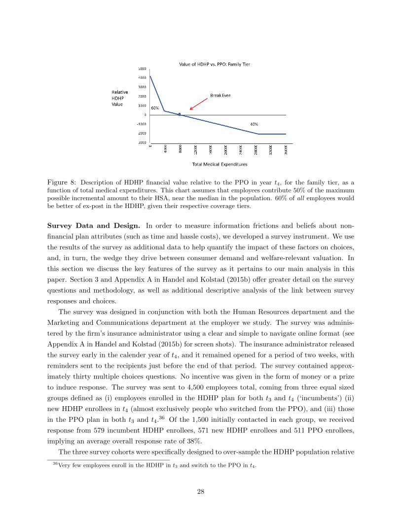
Figure 8: Description of HDHP financial value relative to the PPO in year t4, for the family tier, as afunction of total medical expenditures. This chart assumes that employees contribute 50% of the maximumpossible incremental amount to their HSA, near the median in the population. 60% of all employees wouldbe better of ex-post in the HDHP, given their respective coverage tiers.

Survey Data and Design. In order to measure information frictions and beliefs about non-

financial plan attributes (such as time and hassle costs), we developed a survey instrument. We use

the results of the survey as additional data to help quantify the impact of these factors on choices,

and, in turn, the wedge they drive between consumer demand and welfare-relevant valuation. In

this section we discuss the key features of the survey as it pertains to our main analysis in this

paper. Section 3 and Appendix A in Handel and Kolstad (2015b) offer greater detail on the survey

questions and methodology, as well as additional descriptive analysis of the link between survey

responses and choices.

The survey was designed in conjunction with both the Human Resources department and the

Marketing and Communications department at the employer we study. The survey was adminis-

tered by the firm’s insurance administrator using a clear and simple to navigate online format (see

Appendix A in Handel and Kolstad (2015b) for screen shots). The insurance administrator released

the survey early in the calender year of t4, and it remained opened for a period of two weeks, with

reminders sent to the recipients just before the end of that period. The survey contained approx-

imately thirty multiple choices questions. No incentive was given in the form of money or a prize

to induce response. The survey was sent to 4,500 employees total, coming from three equal sized

groups defined as (i) employees enrolled in the HDHP plan for both t3 and t4 (‘incumbents’) (ii)

new HDHP enrollees in t4 (almost exclusively people who switched from the PPO), and (iii) those

in the PPO plan in both t3 and t4.36 Of the 1,500 initially contacted in each group, we received

response from 579 incumbent HDHP enrollees, 571 new HDHP enrollees and 511 PPO enrollees,

implying an average overall response rate of 38%.

The three survey cohorts were specifically designed to over-sample the HDHP population relative

36Very few employees enroll in the HDHP in t3 and switch to the PPO in t4.

28

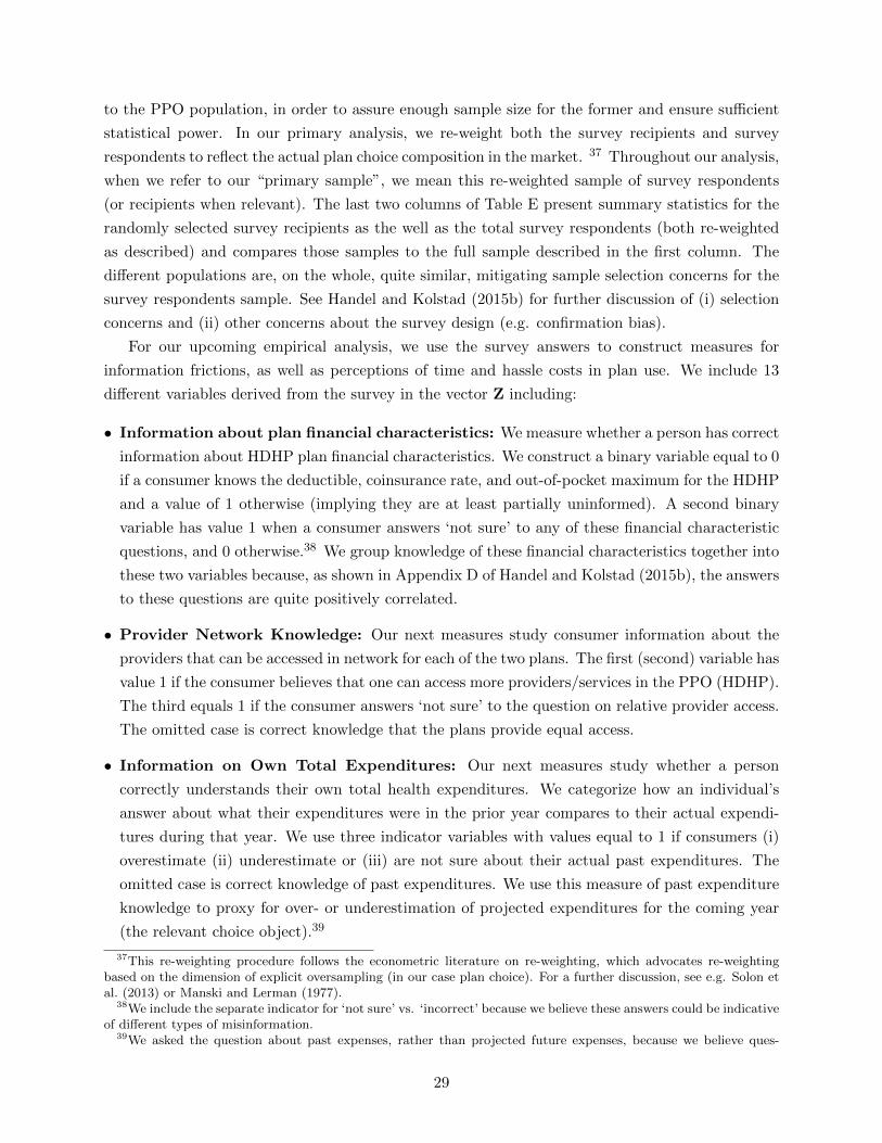
to the PPO population, in order to assure enough sample size for the former and ensure sufficient

statistical power. In our primary analysis, we re-weight both the survey recipients and survey

respondents to reflect the actual plan choice composition in the market. 37 Throughout our analysis,

when we refer to our “primary sample”, we mean this re-weighted sample of survey respondents

(or recipients when relevant). The last two columns of Table E present summary statistics for the

randomly selected survey recipients as the well as the total survey respondents (both re-weighted

as described) and compares those samples to the full sample described in the first column. The

different populations are, on the whole, quite similar, mitigating sample selection concerns for the

survey respondents sample. See Handel and Kolstad (2015b) for further discussion of (i) selection

concerns and (ii) other concerns about the survey design (e.g. confirmation bias).

For our upcoming empirical analysis, we use the survey answers to construct measures for

information frictions, as well as perceptions of time and hassle costs in plan use. We include 13

different variables derived from the survey in the vector Z including:

• Information about plan financial characteristics: We measure whether a person has correct

information about HDHP plan financial characteristics. We construct a binary variable equal to 0

if a consumer knows the deductible, coinsurance rate, and out-of-pocket maximum for the HDHP

and a value of 1 otherwise (implying they are at least partially uninformed). A second binary

variable has value 1 when a consumer answers ‘not sure’ to any of these financial characteristic

questions, and 0 otherwise.38 We group knowledge of these financial characteristics together into

these two variables because, as shown in Appendix D of Handel and Kolstad (2015b), the answers

to these questions are quite positively correlated.

• Provider Network Knowledge: Our next measures study consumer information about the

providers that can be accessed in network for each of the two plans. The first (second) variable has

value 1 if the consumer believes that one can access more providers/services in the PPO (HDHP).

The third equals 1 if the consumer answers ‘not sure’ to the question on relative provider access.

The omitted case is correct knowledge that the plans provide equal access.

• Information on Own Total Expenditures: Our next measures study whether a person

correctly understands their own total health expenditures. We categorize how an individual’s

answer about what their expenditures were in the prior year compares to their actual expendi-

tures during that year. We use three indicator variables with values equal to 1 if consumers (i)

overestimate (ii) underestimate or (iii) are not sure about their actual past expenditures. The

omitted case is correct knowledge of past expenditures. We use this measure of past expenditure

knowledge to proxy for over- or underestimation of projected expenditures for the coming year

(the relevant choice object).39

37This re-weighting procedure follows the econometric literature on re-weighting, which advocates re-weightingbased on the dimension of explicit oversampling (in our case plan choice). For a further discussion, see e.g. Solon etal. (2013) or Manski and Lerman (1977).

38We include the separate indicator for ‘not sure’ vs. ‘incorrect’ because we believe these answers could be indicativeof different types of misinformation.

39We asked the question about past expenses, rather than projected future expenses, because we believe ques-

29

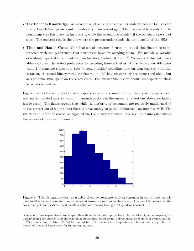
• Tax Benefits Knowledge: We measure whether or not a consumer understands the tax benefits

that a Health Savings Account provides (its main advantage). The first variable equals 1 if the

person answers this question incorrectly, while the second one equals 1 if the person answers ‘not

sure.’ The omitted case is the one where the person understands the tax benefits of the HSA.

• Time and Hassle Costs: Our final set of measures focuses on stated time/hassle costs in-

teracted with the preferences that consumers have for avoiding them. We include a variable

describing expected time spent on plan logistics / administration.40 We interact this with vari-

ables capturing the stated preferences for avoiding these activities. A first binary variable takes

value 1 if someone states that they ‘strongly dislike’ spending time on plan logistics / admin-

istration. A second binary variable takes value 1 if they answer they are ‘concerned about but

accept’ some time spent on these activities. The answer ‘don’t care about’ time spent on these

activities is omitted.

Figure 9 shows the number of correct responses a given consumer in our primary sample gave to all

information related questions about insurance options in the survey (all questions above, excluding

hassle costs). The figure reveals that while the majority of consumers are relatively uninformed (3

or less correct out of 8 questions) there is a reasonably large tail of informed consumers as well. The

variation in informativeness, as signaled via the survey responses, is a key input into quantifying

the impact of frictions on demand.

Figure 9: This histogram shows the number of correct responses a given consumer in our primary samplegave to all information related questions about insurance options in the survey. A value of 0 means that theconsumer got no questions right, while a value of 8 means they got all questions correct.

tions about past expenditures are simpler than those about future projections. In the latter type heterogeneity inunderstanding the question and understanding probabilities could swamp a direct measure of under or overestimation.

40See Handel and Kolstad (2015b) for more detail. The answers to this question are bins of hours, e.g. “6 to 10hours” of time and hassle costs for the upcoming year.

30

4 Empirical Model

Handel and Kolstad (2015b) use the linked administrative and survey data described in the last

section to estimate a choice model that quantifies (i) risk aversion (ii) health risk and (iii) the im-

pact of information frictions on willingness-to-pay for insurance. This type of structural approach

is useful for assessing welfare within the current environment as well as for assessing both market

outcomes and welfare in counterfactual policy environments (e.g., those where consumers choice

frictions are reduced via some policies). In this section, we provide a concise description of the

primary model in that paper, present its estimates, describe how these estimates determine the

micro-foundations in our model and how we construct the key curves necessary for determining

market equilibrium and assessing the implications of friction-reducing and insurer risk-adjustment

policies.41

Choice Model. Our empirical specification studies expected utility maximizing families who

make health plan choices that can depend on (i) ex ante cost risk (ii) risk preferences (iii) infor-

mation frictions (iv) time and hassle costs and (v) an idiosyncratic mean zero preference shock.42

The choice model is estimated based on employee choices for year t4, which are the choices made

concurrently to when the linked survey we use to measure information sets was conducted. We de-

scribe the model here conditional on our ex ante cost projections, which are estimated in a separate

detailed medical cost model described later in this section and in Appendix B.

Denote the family-plan specific distributions of out-of-pocket health expenditures output by the

cost model as Fkj(·). Here, k ∈ K is a family unit, j ∈ J is one of the two health plan options

available at the firm in t4. The baseline model assumes that families’ beliefs about their out-of-

pocket expenditures conform to Fkj(·). Each family has latent utility Ukj for each plan and chooses

the plan j that maximizes Ukj . We assume that Ukj has the following von Neumann-Morgenstern

(vNM) expected utility formulation:

Ukj =

∫ ∞0

fkj(s)uk(Wk, xkj , (Pkj , s))ds

Here, uk(·) is the vNM utility index and s is a realization of out-of-pocket medical expenses from

Fkj(·). Wk denotes family-specific wealth and xkj represents consumption in a given state of the

world (defined below). Pkj is the family-time specific premium for plan j. Formally, in our setting

we define the premium Pk,HDHP as:

Pk,HDHP = −(HSASk + τkHSACk )

41Handel and Kolstad (2015b) estimate a wide range of specifications that illustrate the robustness of the primaryspecification we use in this paper.

42Consumer choices also depend on inertia, which is included in the model below. Handel and Kolstad (2015b)presents some specifications that study the relationship between inertia and information frictions, revealing that thesefactors are closely related but not the same (for either positive of normative predictions). Our counterfactual analysispresumes that consumers are in an active choice environment.

31

HSASk is the firm’s subsidy to each employee’s health savings account (HSA) when they enroll in

the HDHP. This is deterministic conditional on the number of dependents being covered (discussed

in Section 3). HSACk is the incremental contribution a family makes to the HSA, on top of HSASk ,

when they sign up for the HDHP. The value of these contributions is equivalent to the value of

pre-tax dollars relative to post-tax dollars, and thus depends on marginal tax rate τk.43

Given this setup, we follow the literature and assume that families have constant absolute risk

aversion (CARA) preferences implying that, for a given ex post consumption level x:

uk(x) = − 1

γk(XAk )e−γk(XA

k )x

Here, γk is a family-specific risk preference parameter that is known to the family but unobserved

to the econometrician. We model this as a function of employee demographics XAk . The CARA

specification implies that the level of absolute risk aversion −u′′(·)

u′(·) , which equals γ, is constant with

respect to the level of x (and, thus, Wk).

Our primary specification reduces the structural assumptions required to incorporate the impact

of frictions and incorporates our survey data using a reduced form approach (see Handel and Kolstad

(2015b) for a specification that treats frictions in a structural manner as well). To this end we use the

indicator variables derived from survey responses, described in Section 3, as observable measures of

consumer information and perceived hassle costs that imply shifts in value for the HDHP relative to

the PPO. For each friction, one category (corresponding to ‘no friction’, e.g., ‘informed’) is excluded

so that the value shift for the HDHP plan is relative to a frictionless consumer for the measure in

question. Specifically, each included friction variable, denoted Zf from vector Z, shifts the money

at stake for each plan, xj , by an amount βfZf that is assumed constant across all potential health

state realizations s from Fj(·).44

Given this setup, for each ex post state of the world a family’s overall level of consumption x

conditional on a draw s from Fkj(·) is:

xkj = Wk − Pkj − s+ Z’kβ1jt=HDHP + η(XBk )1jt=jt−1 + εkj

Here, 1jt=HDHP is an indicator variable taking on value of one if plan j is the HDHP plan.

η(XBk )1jt=jt−1 captures the impact of inertia distinctly from the impact β of information frictions:

empirically, inertia is identified separately from the active choice impact of information frictions

by comparing the choices between new employees, who make active plan choices by definition, and

existing employees who have a default option and may be impacted by inertia.45 Finally, εkj is a

43We model HSACkt based on actual contributions made by those who sign up for the HDHP. The model yields

a family-specific prediction of incremental HSACk , denoted HSACk , which is inserted into the model such that

Pk,HDHP = HSASk + τkHSACk . Appendix E in Handel and Kolstad (2015b) discusses this model in detail.44To illustrate the setup for including frictions, if variable Z1 is an indicator variable that equals 1 if a consumer is

uninformed about his deductible, then β1 measures the difference in valuation for the HDHP plan, for an uninformedperson, relative to an informed person. The coefficient β1 is a reduced form measure that represents the implicationsof an underlying model of choice under uncertainty with limited information, similar to that presented in Section 2in Handel and Kolstad (2015b).

45This model for inertia assumes that inertia operates similar to a tangible switching cost. Alternatives to this

32

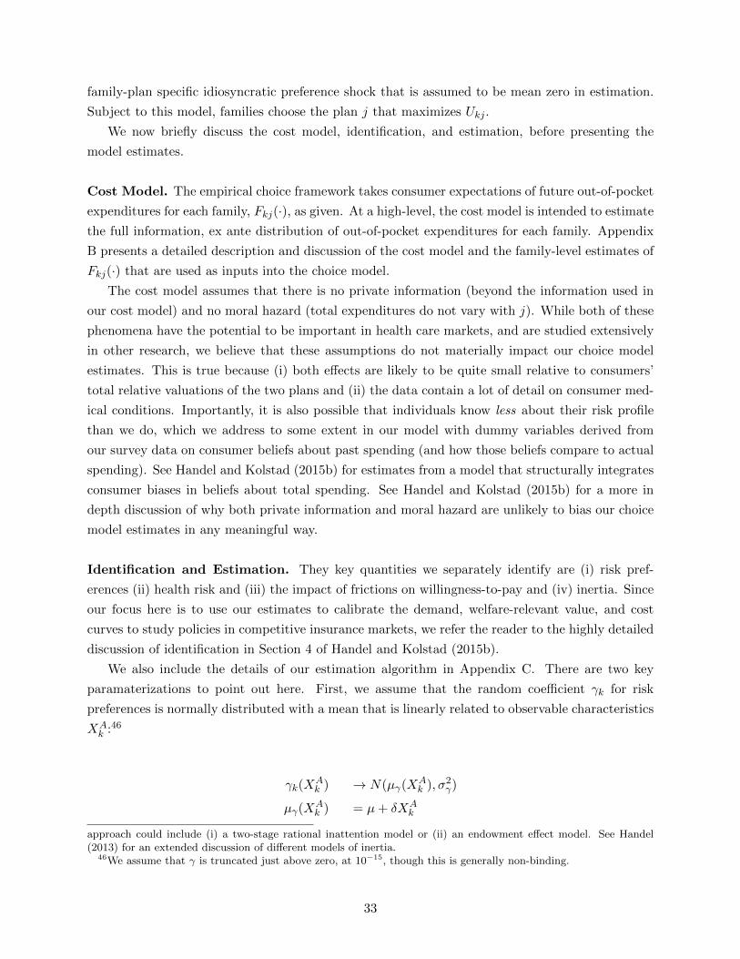
family-plan specific idiosyncratic preference shock that is assumed to be mean zero in estimation.

Subject to this model, families choose the plan j that maximizes Ukj .

We now briefly discuss the cost model, identification, and estimation, before presenting the

model estimates.

Cost Model. The empirical choice framework takes consumer expectations of future out-of-pocket

expenditures for each family, Fkj(·), as given. At a high-level, the cost model is intended to estimate

the full information, ex ante distribution of out-of-pocket expenditures for each family. Appendix

B presents a detailed description and discussion of the cost model and the family-level estimates of

Fkj(·) that are used as inputs into the choice model.

The cost model assumes that there is no private information (beyond the information used in

our cost model) and no moral hazard (total expenditures do not vary with j). While both of these

phenomena have the potential to be important in health care markets, and are studied extensively

in other research, we believe that these assumptions do not materially impact our choice model

estimates. This is true because (i) both effects are likely to be quite small relative to consumers’

total relative valuations of the two plans and (ii) the data contain a lot of detail on consumer med-

ical conditions. Importantly, it is also possible that individuals know less about their risk profile

than we do, which we address to some extent in our model with dummy variables derived from

our survey data on consumer beliefs about past spending (and how those beliefs compare to actual

spending). See Handel and Kolstad (2015b) for estimates from a model that structurally integrates

consumer biases in beliefs about total spending. See Handel and Kolstad (2015b) for a more in

depth discussion of why both private information and moral hazard are unlikely to bias our choice

model estimates in any meaningful way.

Identification and Estimation. They key quantities we separately identify are (i) risk pref-

erences (ii) health risk and (iii) the impact of frictions on willingness-to-pay and (iv) inertia. Since

our focus here is to use our estimates to calibrate the demand, welfare-relevant value, and cost

curves to study policies in competitive insurance markets, we refer the reader to the highly detailed

discussion of identification in Section 4 of Handel and Kolstad (2015b).

We also include the details of our estimation algorithm in Appendix C. There are two key

paramaterizations to point out here. First, we assume that the random coefficient γk for risk

preferences is normally distributed with a mean that is linearly related to observable characteristics

XAk :46

γk(XAk ) → N(µγ(XA

k ), σ2γ)

µγ(XAk ) = µ+ δXA

k

approach could include (i) a two-stage rational inattention model or (ii) an endowment effect model. See Handel(2013) for an extended discussion of different models of inertia.

46We assume that γ is truncated just above zero, at 10−15, though this is generally non-binding.

33

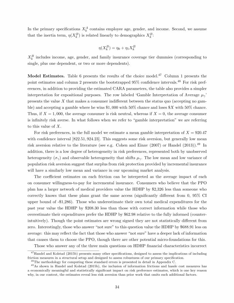
In the primary specifications XAk contains employee age, gender, and income. Second, we assume

that the inertia term, η(XBk ) is related linearly to demographics XB

k :

η(XBk ) = η0 + η1X

Bk

XBk includes income, age, gender, and family insurance coverage tier dummies (corresponding to

single, plus one dependent, or two or more dependents).

Model Estimates. Table 6 presents the results of the choice model.47 Column 1 presents the

point estimates and column 2 presents the bootstrapped 95% confidence intervals.48 For risk pref-

erences, in addition to providing the estimated CARA parameters, the table also provides a simpler

interpretation for expositional purposes. The row labeled ‘Gamble Interpretation of Average µγ ’

presents the value X that makes a consumer indifferent between the status quo (accepting no gam-

ble) and accepting a gamble where he wins $1, 000 with 50% chance and loses $X with 50% chance.

Thus, if X = 1, 000, the average consumer is risk neutral, whereas if X = 0, the average consumer

is infinitely risk averse. In what follows when we refer to “gamble interpretation” we are referring

to this value of X.

For risk preferences, in the full model we estimate a mean gamble interpretation of X = 920.47

with confidence interval [822.51, 924.23]. This suggests some risk aversion, but generally low mean

risk aversion relative to the literature (see e.g. Cohen and Einav (2007) or Handel (2013)).49 In

addition, there is a low degree of heterogeneity in risk preferences, represented both by unobserved

heterogeneity (σγ) and observable heterogeneity that shifts µγ . The low mean and low variance of

population risk aversion suggest that surplus from risk protection provided by incremental insurance

will have a similarly low mean and variance in our upcoming market analysis.

The coefficient estimates on each friction can be interpreted as the average impact of each

on consumer willingness-to-pay for incremental insurance. Consumers who believe that the PPO

plan has a larger network of medical providers value the HDHP by $2,326 less than someone who

correctly knows that these plans grant the same access (significantly different from 0, 95% CI

upper bound of -$1,286). Those who underestimate their own total medical expenditures for the

past year value the HDHP by $208.30 less than those with correct information while those who

overestimate their expenditures prefer the HDHP by $62.98 relative to the fully informed (counter-

intuitively). Though the point estimates are wrong signed they are not statistically different from

zero. Interestingly, those who answer “not sure” to this question value the HDHP by $688.91 less on

average: this may reflect the fact that those who answer “not sure” have a deeper lack of information

that causes them to choose the PPO, though there are other potential micro-foundations for this.

Those who answer any of the three main questions on HDHP financial characteristics incorrect

47Handel and Kolstad (2015b) presents many other specifications, designed to assess the implications of includingfriction measures in a structural setup and designed to assess robustness of our primary specification.

48The methodology for computing these standard errors is presented in detail in Appendix C.49As shown in Handel and Kolstad (2015b), the inclusion of information frictions and hassle cost measures has

a economically meaningful and statistically significant impact on risk preference estimates, which is one key reasonwhy, in our context, the estimates reveal less risk aversion than prior work that omits such additional factors.

34

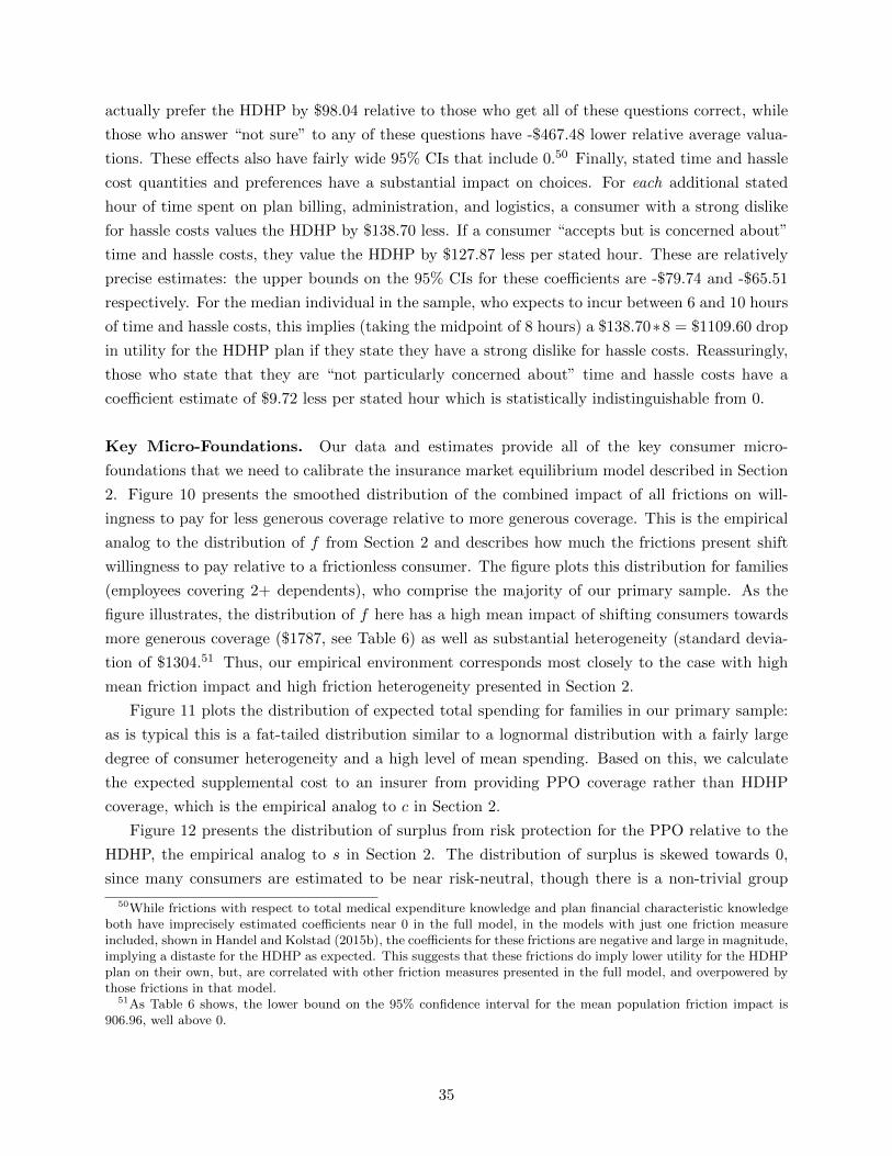
actually prefer the HDHP by $98.04 relative to those who get all of these questions correct, while

those who answer “not sure” to any of these questions have -$467.48 lower relative average valua-

tions. These effects also have fairly wide 95% CIs that include 0.50 Finally, stated time and hassle

cost quantities and preferences have a substantial impact on choices. For each additional stated

hour of time spent on plan billing, administration, and logistics, a consumer with a strong dislike

for hassle costs values the HDHP by $138.70 less. If a consumer “accepts but is concerned about”

time and hassle costs, they value the HDHP by $127.87 less per stated hour. These are relatively

precise estimates: the upper bounds on the 95% CIs for these coefficients are -$79.74 and -$65.51

respectively. For the median individual in the sample, who expects to incur between 6 and 10 hours

of time and hassle costs, this implies (taking the midpoint of 8 hours) a $138.70∗8 = $1109.60 drop

in utility for the HDHP plan if they state they have a strong dislike for hassle costs. Reassuringly,

those who state that they are “not particularly concerned about” time and hassle costs have a

coefficient estimate of $9.72 less per stated hour which is statistically indistinguishable from 0.

Key Micro-Foundations. Our data and estimates provide all of the key consumer micro-

foundations that we need to calibrate the insurance market equilibrium model described in Section

2. Figure 10 presents the smoothed distribution of the combined impact of all frictions on will-

ingness to pay for less generous coverage relative to more generous coverage. This is the empirical

analog to the distribution of f from Section 2 and describes how much the frictions present shift

willingness to pay relative to a frictionless consumer. The figure plots this distribution for families

(employees covering 2+ dependents), who comprise the majority of our primary sample. As the

figure illustrates, the distribution of f here has a high mean impact of shifting consumers towards

more generous coverage ($1787, see Table 6) as well as substantial heterogeneity (standard devia-

tion of $1304.51 Thus, our empirical environment corresponds most closely to the case with high

mean friction impact and high friction heterogeneity presented in Section 2.

Figure 11 plots the distribution of expected total spending for families in our primary sample:

as is typical this is a fat-tailed distribution similar to a lognormal distribution with a fairly large

degree of consumer heterogeneity and a high level of mean spending. Based on this, we calculate

the expected supplemental cost to an insurer from providing PPO coverage rather than HDHP

coverage, which is the empirical analog to c in Section 2.

Figure 12 presents the distribution of surplus from risk protection for the PPO relative to the

HDHP, the empirical analog to s in Section 2. The distribution of surplus is skewed towards 0,

since many consumers are estimated to be near risk-neutral, though there is a non-trivial group

50While frictions with respect to total medical expenditure knowledge and plan financial characteristic knowledgeboth have imprecisely estimated coefficients near 0 in the full model, in the models with just one friction measureincluded, shown in Handel and Kolstad (2015b), the coefficients for these frictions are negative and large in magnitude,implying a distaste for the HDHP as expected. This suggests that these frictions do imply lower utility for the HDHPplan on their own, but, are correlated with other friction measures presented in the full model, and overpowered bythose frictions in that model.

51As Table 6 shows, the lower bound on the 95% confidence interval for the mean population friction impact is906.96, well above 0.

35

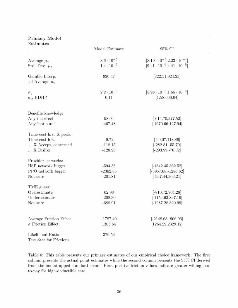
Primary ModelEstimates

Model Estimate 95% CI

Average µγ 8.6 · 10−5 [8.19 · 10−5,2.23 · 10−4]Std. Dev. µγ 1.4 · 10−5 [9.41 · 10−6,4.41 · 10−5]

Gamble Interp. 920.47 [822.51,924.23]of Average µγ

σγ 2.2 · 10−9 [5.98 · 10−6,1.55 · 10−4]σε, HDHP 0.11 [1.58,666.04]

Benefits knowledge:Any incorrect 98.04 [-614.70,377.52]Any ‘not sure’ -467.48 [-1670.66,127.94]

Time cost hrs. X prefs:Time cost hrs. -9.72 [-90.07,118.86]... X Accept, concerned -118.15 [-282.81,-55.79]... X Dislike -128.98 [-293.99,-70.02]

Provider networks:HSP network bigger -594.38 [-1842.45,562.52]PPO network bigger -2362.85 [-3957.68,-1286.62]Not sure -201.81 [-937.44,303.21]

TME guess:Overestimate 62.98 [-810.72,704.28]Underestimate -208.30 [-1154.63,837.19]Not sure -688.91 [-1987.28,320.99]

Average Friction Effect -1787.40 [-2148.63,-906.96]σ Friction Effect 1303.64 [1264.29,2329.12]

Likelihood Ratio 379.54Test Stat for Frictions

Table 6: This table presents our primary estimates of our empirical choice framework. The firstcolumn presents the actual point estimates while the second column presents the 95% CI derivedfrom the bootstrapped standard errors. Here, positive friction values indicate greater willingness-to-pay for high-deductible care.

36

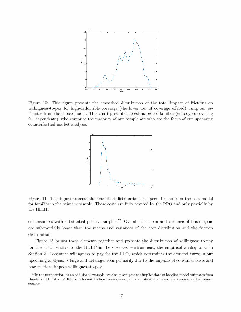
Figure 10: This figure presents the smoothed distribution of the total impact of frictions onwillingness-to-pay for high-deductible coverage (the lower tier of coverage offered) using our es-timates from the choice model. This chart presents the estimates for families (employees covering2+ dependents), who comprise the majority of our sample are who are the focus of our upcomingcounterfactual market analysis.

Figure 11: This figure presents the smoothed distribution of expected costs from the cost modelfor families in the primary sample. These costs are fully covered by the PPO and only partially bythe HDHP.

of consumers with substantial positive surplus.52 Overall, the mean and variance of this surplus

are substantially lower than the means and variances of the cost distribution and the friction

distribution.

Figure 13 brings these elements together and presents the distribution of willingness-to-pay

for the PPO relative to the HDHP in the observed environment, the empirical analog to w in

Section 2. Consumer willingness to pay for the PPO, which determines the demand curve in our

upcoming analysis, is large and heterogeneous primarily due to the impacts of consumer costs and

how frictions impact willingness-to-pay.

52In the next section, as an additional example, we also investigate the implications of baseline model estimates fromHandel and Kolstad (2015b) which omit friction measures and show substantially larger risk aversion and consumersurplus.

37

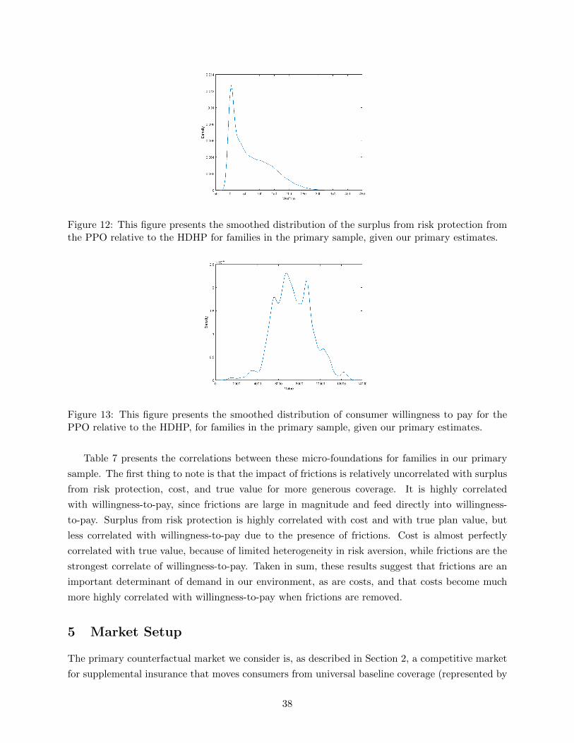
Figure 12: This figure presents the smoothed distribution of the surplus from risk protection fromthe PPO relative to the HDHP for families in the primary sample, given our primary estimates.

Figure 13: This figure presents the smoothed distribution of consumer willingness to pay for thePPO relative to the HDHP, for families in the primary sample, given our primary estimates.

Table 7 presents the correlations between these micro-foundations for families in our primary

sample. The first thing to note is that the impact of frictions is relatively uncorrelated with surplus

from risk protection, cost, and true value for more generous coverage. It is highly correlated

with willingness-to-pay, since frictions are large in magnitude and feed directly into willingness-

to-pay. Surplus from risk protection is highly correlated with cost and with true plan value, but

less correlated with willingness-to-pay due to the presence of frictions. Cost is almost perfectly

correlated with true value, because of limited heterogeneity in risk aversion, while frictions are the

strongest correlate of willingness-to-pay. Taken in sum, these results suggest that frictions are an

important determinant of demand in our environment, as are costs, and that costs become much

more highly correlated with willingness-to-pay when frictions are removed.

5 Market Setup

The primary counterfactual market we consider is, as described in Section 2, a competitive market

for supplemental insurance that moves consumers from universal baseline coverage (represented by

38

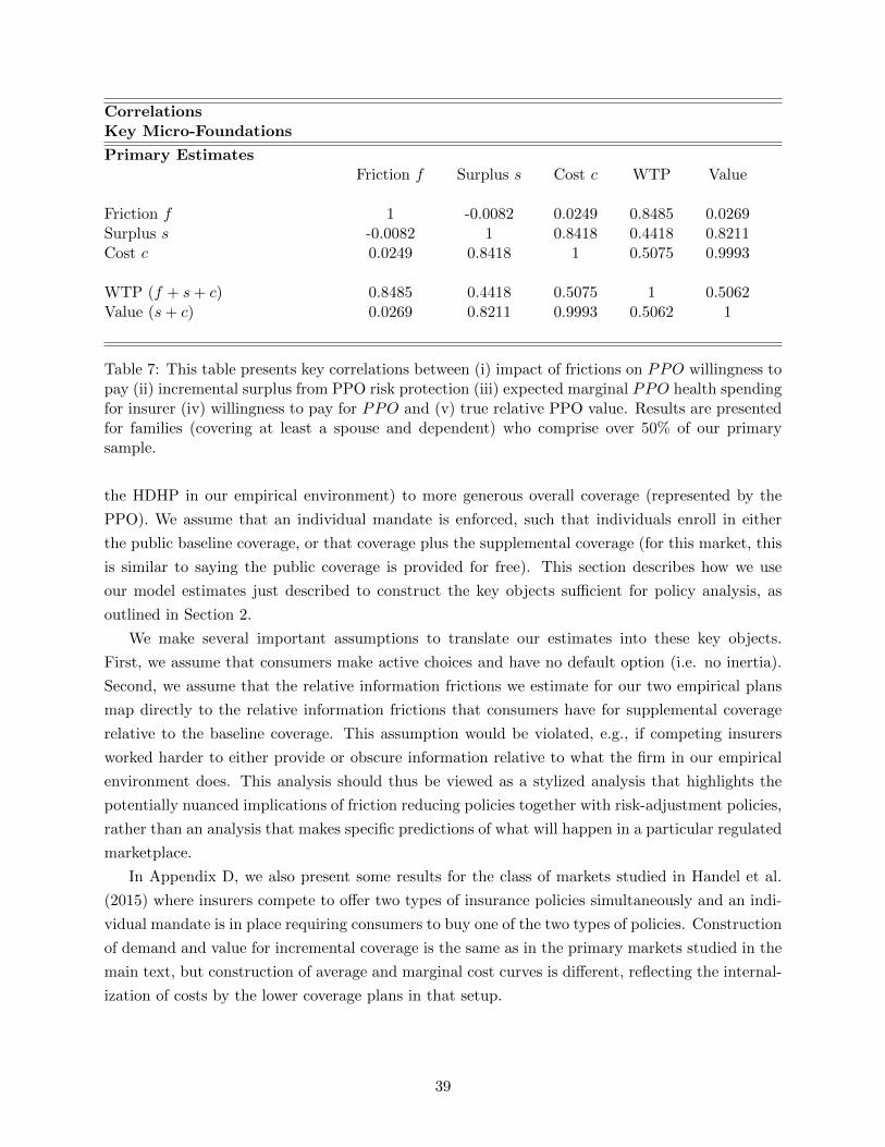
CorrelationsKey Micro-Foundations

Primary EstimatesFriction f Surplus s Cost c WTP Value

Friction f 1 -0.0082 0.0249 0.8485 0.0269Surplus s -0.0082 1 0.8418 0.4418 0.8211Cost c 0.0249 0.8418 1 0.5075 0.9993

WTP (f + s+ c) 0.8485 0.4418 0.5075 1 0.5062Value (s+ c) 0.0269 0.8211 0.9993 0.5062 1

Table 7: This table presents key correlations between (i) impact of frictions on PPO willingness topay (ii) incremental surplus from PPO risk protection (iii) expected marginal PPO health spendingfor insurer (iv) willingness to pay for PPO and (v) true relative PPO value. Results are presentedfor families (covering at least a spouse and dependent) who comprise over 50% of our primarysample.

the HDHP in our empirical environment) to more generous overall coverage (represented by the

PPO). We assume that an individual mandate is enforced, such that individuals enroll in either

the public baseline coverage, or that coverage plus the supplemental coverage (for this market, this

is similar to saying the public coverage is provided for free). This section describes how we use

our model estimates just described to construct the key objects sufficient for policy analysis, as

outlined in Section 2.

We make several important assumptions to translate our estimates into these key objects.

First, we assume that consumers make active choices and have no default option (i.e. no inertia).

Second, we assume that the relative information frictions we estimate for our two empirical plans

map directly to the relative information frictions that consumers have for supplemental coverage

relative to the baseline coverage. This assumption would be violated, e.g., if competing insurers

worked harder to either provide or obscure information relative to what the firm in our empirical

environment does. This analysis should thus be viewed as a stylized analysis that highlights the

potentially nuanced implications of friction reducing policies together with risk-adjustment policies,

rather than an analysis that makes specific predictions of what will happen in a particular regulated

marketplace.

In Appendix D, we also present some results for the class of markets studied in Handel et al.

(2015) where insurers compete to offer two types of insurance policies simultaneously and an indi-

vidual mandate is in place requiring consumers to buy one of the two types of policies. Construction

of demand and value for incremental coverage is the same as in the primary markets studied in the

main text, but construction of average and marginal cost curves is different, reflecting the internal-

ization of costs by the lower coverage plans in that setup.

39

Demand, Value, and Cost Curves. We study a range of demand-side policies that reduce

consumer choice frictions and supply-side policies that impact the costs insurers face for different

consumers. Using our structural estimates of frictions, surplus and costs we construct (i) demand

curve (ii) welfare-relevant value curve and (iii) average and marginal cost curves for each policy

scenario.

The demand curve reflects consumer willingness-to-pay for more generous coverage in a given

policy environment. This willingness-to-pay is the same regardless of whether it is a market for

supplemental add-on coverage or a market where insurers offer both types of plans. Of the two

policies we consider here — those that reduce information frictions and insurer risk adjustment

transfers — only the former impacts consumer demand. As a result, counterfactual consumer

willingness-to-pay for each plan j given a specific information friction reduction policy α is:

Ukj(α) =

∫ ∞0

fkj(s)−1

γk(XAk )e−γk(XA

k )xkj(α,s)ds

xkj(α, s) = Wk − Pkj − s+ (1− α)Z’kβ1jt=HDHP + η(XBk )1jt=jt−1 + ˆεkj

Thus, when α = 0 all information frictions are present and consumer demand is composed of

estimated willingness-to-pay for each plan in our given environment. When α > 0 then information

frictions are reduced by some fraction, up to the case when α = 1 and 100% of frictions are removed.

In our upcoming analysis, we investigate a space of policies corresponding to values of α between

0 and 1. The level of α can be thought of as a reduced form representation of different policy

combinations that reduce consumer choice frictions (e.g. information provision, decision support,

or smart defaults). Though we do not quantify the empirical impact of actual friction-reducing

policies in this paper, one could in principle study values of α linked to specific empirical measures

and/or policy changes.

We define willingness-to-pay for the PPO, relative to the HDHP, as the difference in certainty

equivalents implied by the above utility model:

wk(α) = CEk,PPO(α)− CEk,HDHP (α) (5)

Here, wk is family k’s relative willingness to pay, and CEk,x is the certain financial payment that

gives equivalent utility to that families’ utility from choosing plan x.

The corresponding relative demand curve reflects willingness to pay for the PPO relative to

the HDHP given the friction-reducing implications of α:

D(P ;α) = Pr(wk(α) ≥ P )

Here, P is the price of supplemental coverage that moves the consumer from the baseline HDHP plan

to combined coverage represented by the PPO plan. We use this demand curve for our equilibrium

analysis of counterfactual policies with specific values of α.

40

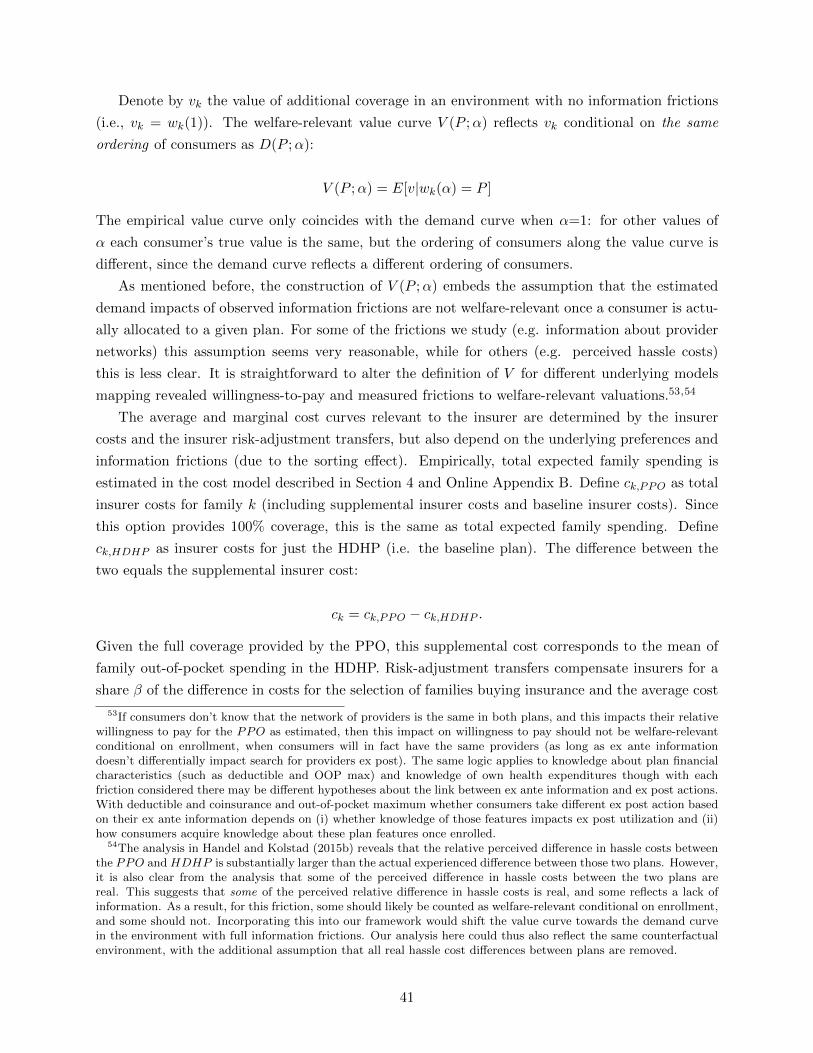
Denote by vk the value of additional coverage in an environment with no information frictions

(i.e., vk = wk(1)). The welfare-relevant value curve V (P ;α) reflects vk conditional on the same

ordering of consumers as D(P ;α):

V (P ;α) = E[v|wk(α) = P ]

The empirical value curve only coincides with the demand curve when α=1: for other values of

α each consumer’s true value is the same, but the ordering of consumers along the value curve is

different, since the demand curve reflects a different ordering of consumers.

As mentioned before, the construction of V (P ;α) embeds the assumption that the estimated

demand impacts of observed information frictions are not welfare-relevant once a consumer is actu-

ally allocated to a given plan. For some of the frictions we study (e.g. information about provider

networks) this assumption seems very reasonable, while for others (e.g. perceived hassle costs)

this is less clear. It is straightforward to alter the definition of V for different underlying models

mapping revealed willingness-to-pay and measured frictions to welfare-relevant valuations.53,54

The average and marginal cost curves relevant to the insurer are determined by the insurer

costs and the insurer risk-adjustment transfers, but also depend on the underlying preferences and

information frictions (due to the sorting effect). Empirically, total expected family spending is

estimated in the cost model described in Section 4 and Online Appendix B. Define ck,PPO as total

insurer costs for family k (including supplemental insurer costs and baseline insurer costs). Since

this option provides 100% coverage, this is the same as total expected family spending. Define

ck,HDHP as insurer costs for just the HDHP (i.e. the baseline plan). The difference between the

two equals the supplemental insurer cost:

ck = ck,PPO − ck,HDHP .

Given the full coverage provided by the PPO, this supplemental cost corresponds to the mean of

family out-of-pocket spending in the HDHP. Risk-adjustment transfers compensate insurers for a

share β of the difference in costs for the selection of families buying insurance and the average cost

53If consumers don’t know that the network of providers is the same in both plans, and this impacts their relativewillingness to pay for the PPO as estimated, then this impact on willingness to pay should not be welfare-relevantconditional on enrollment, when consumers will in fact have the same providers (as long as ex ante informationdoesn’t differentially impact search for providers ex post). The same logic applies to knowledge about plan financialcharacteristics (such as deductible and OOP max) and knowledge of own health expenditures though with eachfriction considered there may be different hypotheses about the link between ex ante information and ex post actions.With deductible and coinsurance and out-of-pocket maximum whether consumers take different ex post action basedon their ex ante information depends on (i) whether knowledge of those features impacts ex post utilization and (ii)how consumers acquire knowledge about these plan features once enrolled.

54The analysis in Handel and Kolstad (2015b) reveals that the relative perceived difference in hassle costs betweenthe PPO and HDHP is substantially larger than the actual experienced difference between those two plans. However,it is also clear from the analysis that some of the perceived difference in hassle costs between the two plans arereal. This suggests that some of the perceived relative difference in hassle costs is real, and some reflects a lack ofinformation. As a result, for this friction, some should likely be counted as welfare-relevant conditional on enrollment,and some should not. Incorporating this into our framework would shift the value curve towards the demand curvein the environment with full information frictions. Our analysis here could thus also reflect the same counterfactualenvironment, with the additional assumption that all real hassle cost differences between plans are removed.

41

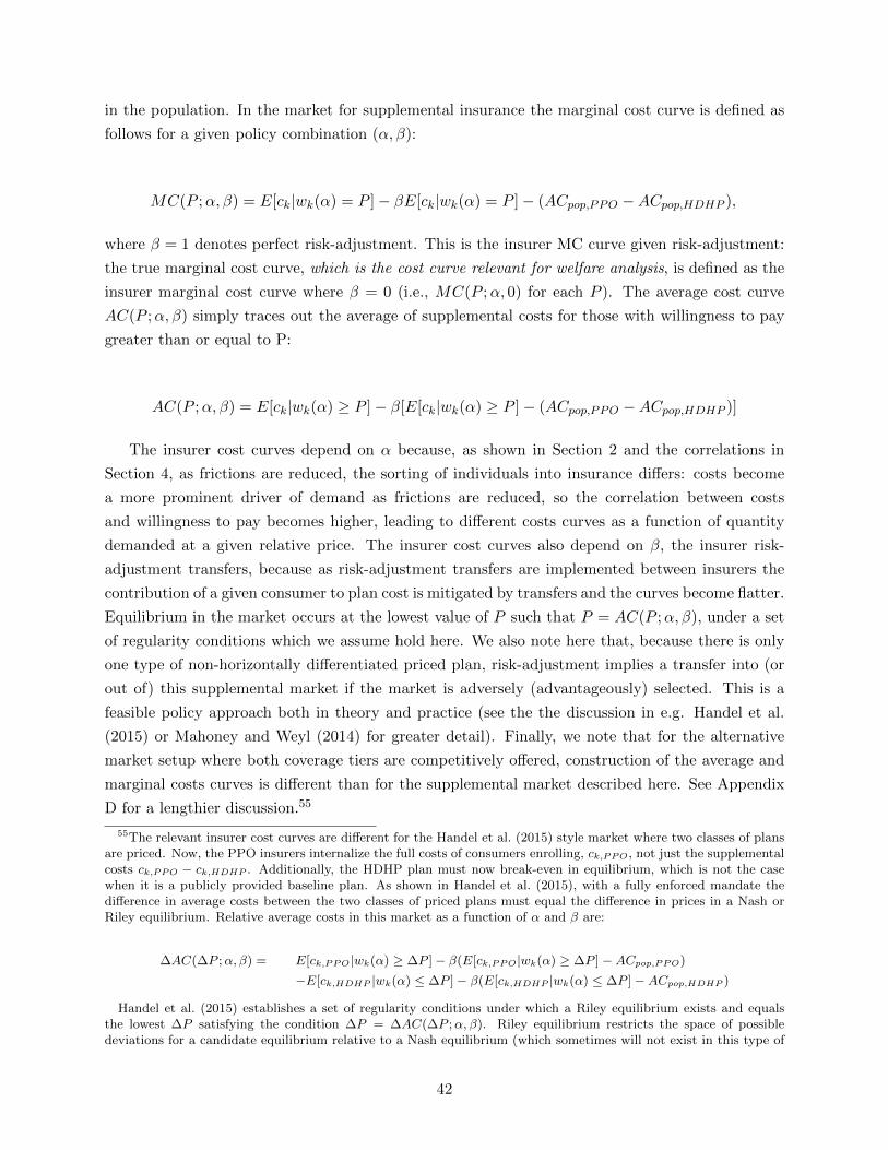
in the population. In the market for supplemental insurance the marginal cost curve is defined as

follows for a given policy combination (α, β):

MC(P ;α, β) = E[ck|wk(α) = P ]− βE[ck|wk(α) = P ]− (ACpop,PPO −ACpop,HDHP ),

where β = 1 denotes perfect risk-adjustment. This is the insurer MC curve given risk-adjustment:

the true marginal cost curve, which is the cost curve relevant for welfare analysis, is defined as the

insurer marginal cost curve where β = 0 (i.e., MC(P ;α, 0) for each P ). The average cost curve

AC(P ;α, β) simply traces out the average of supplemental costs for those with willingness to pay

greater than or equal to P:

AC(P ;α, β) = E[ck|wk(α) ≥ P ]− β[E[ck|wk(α) ≥ P ]− (ACpop,PPO −ACpop,HDHP )]

The insurer cost curves depend on α because, as shown in Section 2 and the correlations in

Section 4, as frictions are reduced, the sorting of individuals into insurance differs: costs become

a more prominent driver of demand as frictions are reduced, so the correlation between costs

and willingness to pay becomes higher, leading to different costs curves as a function of quantity

demanded at a given relative price. The insurer cost curves also depend on β, the insurer risk-

adjustment transfers, because as risk-adjustment transfers are implemented between insurers the

contribution of a given consumer to plan cost is mitigated by transfers and the curves become flatter.

Equilibrium in the market occurs at the lowest value of P such that P = AC(P ;α, β), under a set

of regularity conditions which we assume hold here. We also note here that, because there is only

one type of non-horizontally differentiated priced plan, risk-adjustment implies a transfer into (or

out of) this supplemental market if the market is adversely (advantageously) selected. This is a

feasible policy approach both in theory and practice (see the the discussion in e.g. Handel et al.

(2015) or Mahoney and Weyl (2014) for greater detail). Finally, we note that for the alternative

market setup where both coverage tiers are competitively offered, construction of the average and

marginal costs curves is different than for the supplemental market described here. See Appendix

D for a lengthier discussion.55

55The relevant insurer cost curves are different for the Handel et al. (2015) style market where two classes of plansare priced. Now, the PPO insurers internalize the full costs of consumers enrolling, ck,PPO, not just the supplementalcosts ck,PPO − ck,HDHP . Additionally, the HDHP plan must now break-even in equilibrium, which is not the casewhen it is a publicly provided baseline plan. As shown in Handel et al. (2015), with a fully enforced mandate thedifference in average costs between the two classes of priced plans must equal the difference in prices in a Nash orRiley equilibrium. Relative average costs in this market as a function of α and β are:

∆AC(∆P ;α, β) = E[ck,PPO|wk(α) ≥ ∆P ]− β(E[ck,PPO|wk(α) ≥ ∆P ]−ACpop,PPO)

−E[ck,HDHP |wk(α) ≤ ∆P ]− β(E[ck,HDHP |wk(α) ≤ ∆P ]−ACpop,HDHP )

Handel et al. (2015) establishes a set of regularity conditions under which a Riley equilibrium exists and equalsthe lowest ∆P satisfying the condition ∆P = ∆AC(∆P ;α, β). Riley equilibrium restricts the space of possibledeviations for a candidate equilibrium relative to a Nash equilibrium (which sometimes will not exist in this type of

42

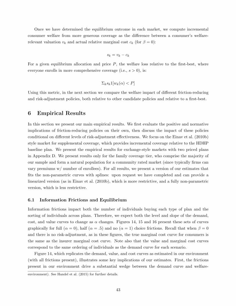
Once we have determined the equilibrium outcome in each market, we compute incremental

consumer welfare from more generous coverage as the difference between a consumer’s welfare-

relevant valuation vk and actual relative marginal cost ck (for β = 0):

sk = vk − ck

For a given equilibrium allocation and price P , the welfare loss relative to the first-best, where

everyone enrolls in more comprehensive coverage (i.e., s > 0), is:

Σksk1[wk(α) < P ]

Using this metric, in the next section we compare the welfare impact of different friction-reducing

and risk-adjustment policies, both relative to other candidate policies and relative to a first-best.

6 Empirical Results

In this section we present our main empirical results. We first evaluate the positive and normative

implications of friction-reducing policies on their own, then discuss the impact of these policies

conditional on different levels of risk-adjustment effectiveness. We focus on the Einav et al. (2010b)

style market for supplemental coverage, which provides incremental coverage relative to the HDHP

baseline plan. We present the empirical results for exchange-style markets with two priced plans

in Appendix D. We present results only for the family coverage tier, who comprise the majority of

our sample and form a natural population for a community rated market (since typically firms can

vary premiums w/ number of enrollees). For all results, we present a version of our estimates that

fits the non-parametric curves with splines: upon request we have completed and can provide a

linearized version (as in Einav et al. (2010b), which is more restrictive, and a fully non-parametric

version, which is less restrictive.

6.1 Information Frictions and Equilibrium

Information frictions impact both the number of individuals buying each type of plan and the

sorting of individuals across plans. Therefore, we expect both the level and slope of the demand,

cost, and value curves to change as α changes. Figures 14, 15 and 16 present these sets of curves

graphically for full (α = 0), half (α = .5) and no (α = 1) choice frictions. Recall that when β = 0

and there is no risk-adjustment, as in these figures, the true marginal cost curve for consumers is

the same as the insurer marginal cost curve. Note also that the value and marginal cost curves

correspond to the same ordering of individuals as the demand curve for each scenario.

Figure 14, which replicates the demand, value, and cost curves as estimated in our environment

(with all frictions present), illustrates some key implications of our estimates. First, the frictions

present in our environment drive a substantial wedge between the demand curve and welfare-

environment). See Handel et al. (2015) for further details.

43

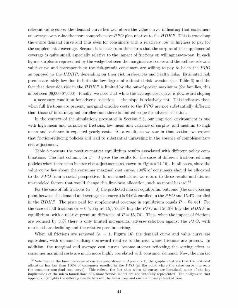
relevant value curve: the demand curve lies well above the value curve, indicating that consumers

on average over-value the more comprehensive PPO plan relative to the HDHP . This is true along

the entire demand curve and thus even for consumers with a relatively low willingness to pay for

the supplemental coverage. Second, it is clear from the charts that the surplus of the supplemental

coverage is quite small, especially relative to the impact of frictions on willingness-to-pay. In each

figure, surplus is represented by the wedge between the marginal cost curve and the welfare-relevant

value curve and corresponds to the risk-premia consumers are willing to pay to be in the PPO

as opposed to the HDHP , depending on their risk preferences and health risks. Estimated risk

premia are fairly low due to both the low degree of estimated risk aversion (see Table 6) and the

fact that downside risk in the HDHP is limited by the out-of-pocket maximum (for families, this

is between $6,000-$7,000). Finally, we note that while the average cost curve is downward sloping

— a necessary condition for adverse selection — the slope is relatively flat. This indicates that,

when full frictions are present, marginal enrollee costs to the PPO are not substantially different

than those of infra-marginal enrollees and there is limited scope for adverse selection.

In the context of the simulations presented in Section 2.5, our empirical environment is one

with high mean and variance of frictions, low mean and variance of surplus, and medium to high

mean and variance in expected yearly costs. As a result, as we saw in that section, we expect

that friction-reducing policies will lead to substantial unraveling in the absence of complementary

risk-adjustment.

Table 8 presents the positive market equilibrium results associated with different policy com-

binations. The first column, for β = 0 gives the results for the cases of different friction-reducing

policies when there is no insurer risk-adjustment (as shown in Figures 14-16). In all cases, since the

value curve lies about the consumer marginal cost curve, 100% of consumers should be allocated

to the PPO from a social perspective. In our conclusions, we return to these results and discuss

un-modeled factors that would change this first-best allocation, such as moral hazard.56

For the case of full frictions (α = 0) the predicted market equilibrium outcome (the one crossing

point between the demand and average cost curves) is 84.6% enrolled in the PPO and 15.4% enrolled

in the HDHP . The price paid for supplemental coverage in equilibrium equals P = $5, 551. For

the case of half frictions (α = 0.5, Figure 15), 73.4% buy the PPO and 26.6% buy the HDHP in

equilibrium, with a relative premium difference of P = $5, 741. Thus, when the impact of frictions

are reduced by 50% there is only limited incremental adverse selection against the PPO, with

market share declining and the relative premium rising.

When all frictions are removed (α = 1, Figure 16) the demand curve and value curve are

equivalent, with demand shifting downward relative to the case where frictions are present. In

addition, the marginal and average cost curves become steeper reflecting the sorting effect as

consumer marginal costs are much more highly correlated with consumer demand. Now, the market

56Note that in the linear versions of our analysis, shown in Appendix E, the graphs illustrate that the first-bestallocation has less than 100% of consumers enrolled in the PPO (at the point where the value curve intersectsthe consumer marginal cost curve). This reflects the fact then when all curves are linearized, some of the keyimplications of the micro-foundations of a more flexible model are not faithfully represented. The analysis in thatappendix highlights the differing results between the linear case and our main case presented here.

44

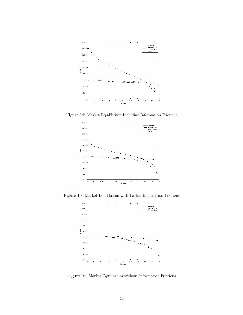
Figure 14: Market Equilibrium Including Information Frictions

Figure 15: Market Equilibrium with Partial Information Frictions

Figure 16: Market Equilibrium without Information Frictions

45

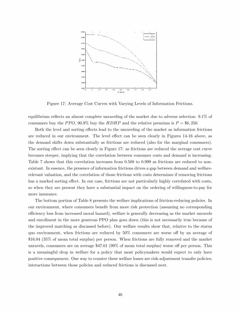
Figure 17: Average Cost Curves with Varying Levels of Information Frictions.

equilibrium reflects an almost complete unraveling of the market due to adverse selection: 9.1% of

consumers buy the PPO, 90.9% buy the HDHP and the relative premium is P = $6, 250.

Both the level and sorting effects lead to the unraveling of the market as information frictions

are reduced in our environment. The level effect can be seen clearly in Figures 14-16 above, as

the demand shifts down substantially as frictions are reduced (also for the marginal consumers).

The sorting effect can be seen clearly in Figure 17: as frictions are reduced the average cost curve

becomes steeper, implying that the correlation between consumer costs and demand is increasing.

Table 7 shows that this correlation increases from 0.508 to 0.999 as frictions are reduced to non-

existant. In essence, the presence of information frictions drives a gap between demand and welfare-

relevant valuation, and the correlation of those frictions with costs determines if removing frictions

has a marked sorting effect. In our case, frictions are not particularly highly correlated with costs,

so when they are present they have a substantial impact on the ordering of willingness-to-pay for

more insurance.

The bottom portion of Table 8 presents the welfare implications of friction-reducing policies. In

our environment, where consumers benefit from more risk protection (assuming no corresponding

efficiency loss from increased moral hazard), welfare is generally decreasing as the market unravels

and enrollment in the more generous PPO plan goes down (this is not necessarily true because of

the improved matching as discussed before). Our welfare results show that, relative to the status

quo environment, when frictions are reduced by 50% consumers are worse off by an average of

$16.04 (35% of mean total surplus) per person. When frictions are fully removed and the market

unravels, consumers are on average $47.01 (99% of mean total surplus) worse off per person. This

is a meaningful drop in welfare for a policy that most policymakers would expect to only have

positive consequences. One way to counter these welfare losses are risk-adjustment transfer policies;

interactions between those policies and reduced frictions is discussed next.

46

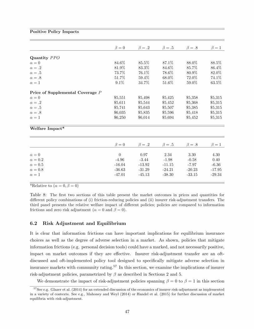
Positive Policy Impacts

β = 0 β = .2 β = .5 β = .8 β = 1

Quantity PPOα = 0 84.6% 85.5% 87.1% 88.0% 88.5%α = .2 81.9% 83.3% 84.6% 85.7% 86.4%α = .5 73.7% 76.1% 78.6% 80.9% 82.0%α = .8 51.7% 59.4% 68.0% 72.0% 74.1%α = 1 9.1% 34.7% 51.6% 59.0% 63.5%

Price of Supplemental Coverage Pα = 0 $5,551 $5,498 $5,425 $5,358 $5,315α = .2 $5,611 $5,544 $5,452 $5,368 $5,315α = .5 $5,741 $5,643 $5,507 $5,385 $5,315α = .8 $6,035 $5,835 $5,596 $5,418 $5,315α = 1 $6,250 $6,014 $5,694 $5,452 $5,315

Welfare Impact*

β = 0 β = .2 β = .5 β = .8 β = 1

α = 0 0 0.97 2.34 3.30 4.30α = 0.2 -4.96 -3.44 -1.98 -0.58 0.40α = 0.5 -16.04 -13.92 -11.15 -7.97 -6.36α = 0.8 -36.63 -31.29 -24.21 -20.23 -17.95α = 1 -47.01 -45.13 -38.30 -33.15 -29.34

*Relative to (α = 0, β = 0)

Table 8: The first two sections of this table present the market outcomes in prices and quantities fordifferent policy combinations of (i) friction-reducing policies and (ii) insurer risk-adjustment transfers. Thethird panel presents the relative welfare impact of different policies; policies are compared to informationfrictions and zero risk adjustment (α = 0 and β = 0).

6.2 Risk Adjustment and Equilibrium

It is clear that information frictions can have important implications for equilibrium insurance

choices as well as the degree of adverse selection in a market. As shown, policies that mitigate

information frictions (e.g. personal decision tools) could have a marked, and not necessarily positive,

impact on market outcomes if they are effective. Insurer risk-adjustment transfer are an oft-

discussed and oft-implemented policy tool designed to specifically mitigate adverse selection in

insurance markets with community rating.57 In this section, we examine the implications of insurer

risk-adjustment policies, parametrized by β as described in Sections 2 and 5.

We demonstrate the impact of risk-adjustment policies spanning β = 0 to β = 1 in this section

57See e.g. Glazer et al. (2014) for an extended discussion of the economics of insurer risk-adjustment as implementedin a variety of contexts. See e.g., Mahoney and Weyl (2014) or Handel et al. (2015) for further discussion of marketequilibria with risk-adjustment.

47

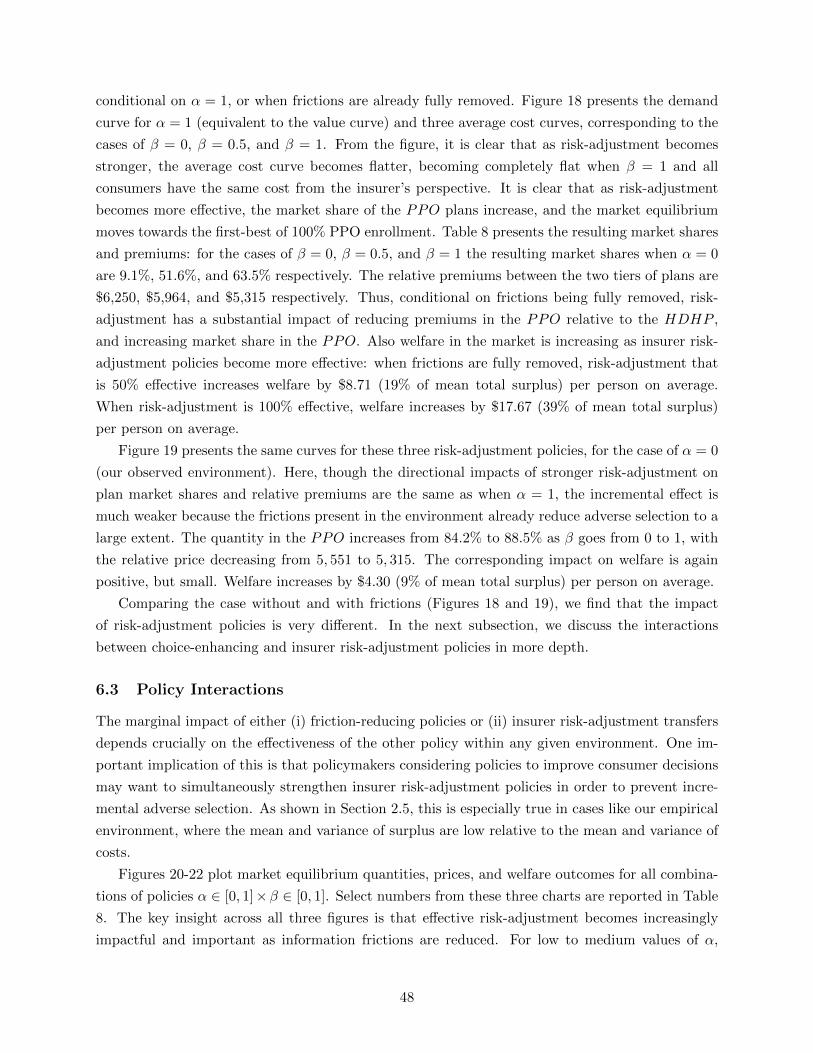
conditional on α = 1, or when frictions are already fully removed. Figure 18 presents the demand

curve for α = 1 (equivalent to the value curve) and three average cost curves, corresponding to the

cases of β = 0, β = 0.5, and β = 1. From the figure, it is clear that as risk-adjustment becomes

stronger, the average cost curve becomes flatter, becoming completely flat when β = 1 and all

consumers have the same cost from the insurer’s perspective. It is clear that as risk-adjustment

becomes more effective, the market share of the PPO plans increase, and the market equilibrium

moves towards the first-best of 100% PPO enrollment. Table 8 presents the resulting market shares

and premiums: for the cases of β = 0, β = 0.5, and β = 1 the resulting market shares when α = 0

are 9.1%, 51.6%, and 63.5% respectively. The relative premiums between the two tiers of plans are

$6,250, $5,964, and $5,315 respectively. Thus, conditional on frictions being fully removed, risk-

adjustment has a substantial impact of reducing premiums in the PPO relative to the HDHP ,

and increasing market share in the PPO. Also welfare in the market is increasing as insurer risk-

adjustment policies become more effective: when frictions are fully removed, risk-adjustment that

is 50% effective increases welfare by $8.71 (19% of mean total surplus) per person on average.

When risk-adjustment is 100% effective, welfare increases by $17.67 (39% of mean total surplus)

per person on average.

Figure 19 presents the same curves for these three risk-adjustment policies, for the case of α = 0

(our observed environment). Here, though the directional impacts of stronger risk-adjustment on

plan market shares and relative premiums are the same as when α = 1, the incremental effect is

much weaker because the frictions present in the environment already reduce adverse selection to a

large extent. The quantity in the PPO increases from 84.2% to 88.5% as β goes from 0 to 1, with

the relative price decreasing from 5, 551 to 5, 315. The corresponding impact on welfare is again

positive, but small. Welfare increases by $4.30 (9% of mean total surplus) per person on average.

Comparing the case without and with frictions (Figures 18 and 19), we find that the impact

of risk-adjustment policies is very different. In the next subsection, we discuss the interactions

between choice-enhancing and insurer risk-adjustment policies in more depth.

6.3 Policy Interactions

The marginal impact of either (i) friction-reducing policies or (ii) insurer risk-adjustment transfers

depends crucially on the effectiveness of the other policy within any given environment. One im-

portant implication of this is that policymakers considering policies to improve consumer decisions

may want to simultaneously strengthen insurer risk-adjustment policies in order to prevent incre-

mental adverse selection. As shown in Section 2.5, this is especially true in cases like our empirical

environment, where the mean and variance of surplus are low relative to the mean and variance of

costs.

Figures 20-22 plot market equilibrium quantities, prices, and welfare outcomes for all combina-

tions of policies α ∈ [0, 1]×β ∈ [0, 1]. Select numbers from these three charts are reported in Table

8. The key insight across all three figures is that effective risk-adjustment becomes increasingly

impactful and important as information frictions are reduced. For low to medium values of α,

48

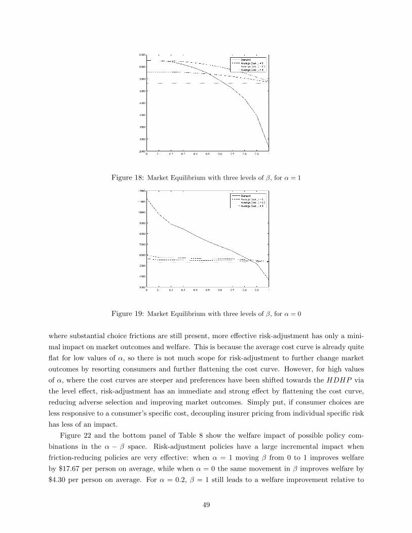
Figure 18: Market Equilibrium with three levels of β, for α = 1

Figure 19: Market Equilibrium with three levels of β, for α = 0

where substantial choice frictions are still present, more effective risk-adjustment has only a mini-

mal impact on market outcomes and welfare. This is because the average cost curve is already quite

flat for low values of α, so there is not much scope for risk-adjustment to further change market

outcomes by resorting consumers and further flattening the cost curve. However, for high values

of α, where the cost curves are steeper and preferences have been shifted towards the HDHP via

the level effect, risk-adjustment has an immediate and strong effect by flattening the cost curve,

reducing adverse selection and improving market outcomes. Simply put, if consumer choices are

less responsive to a consumer’s specific cost, decoupling insurer pricing from individual specific risk

has less of an impact.

Figure 22 and the bottom panel of Table 8 show the welfare impact of possible policy com-

binations in the α − β space. Risk-adjustment policies have a large incremental impact when

friction-reducing policies are very effective: when α = 1 moving β from 0 to 1 improves welfare

by $17.67 per person on average, while when α = 0 the same movement in β improves welfare by

$4.30 per person on average. For α = 0.2, β = 1 still leads to a welfare improvement relative to

49

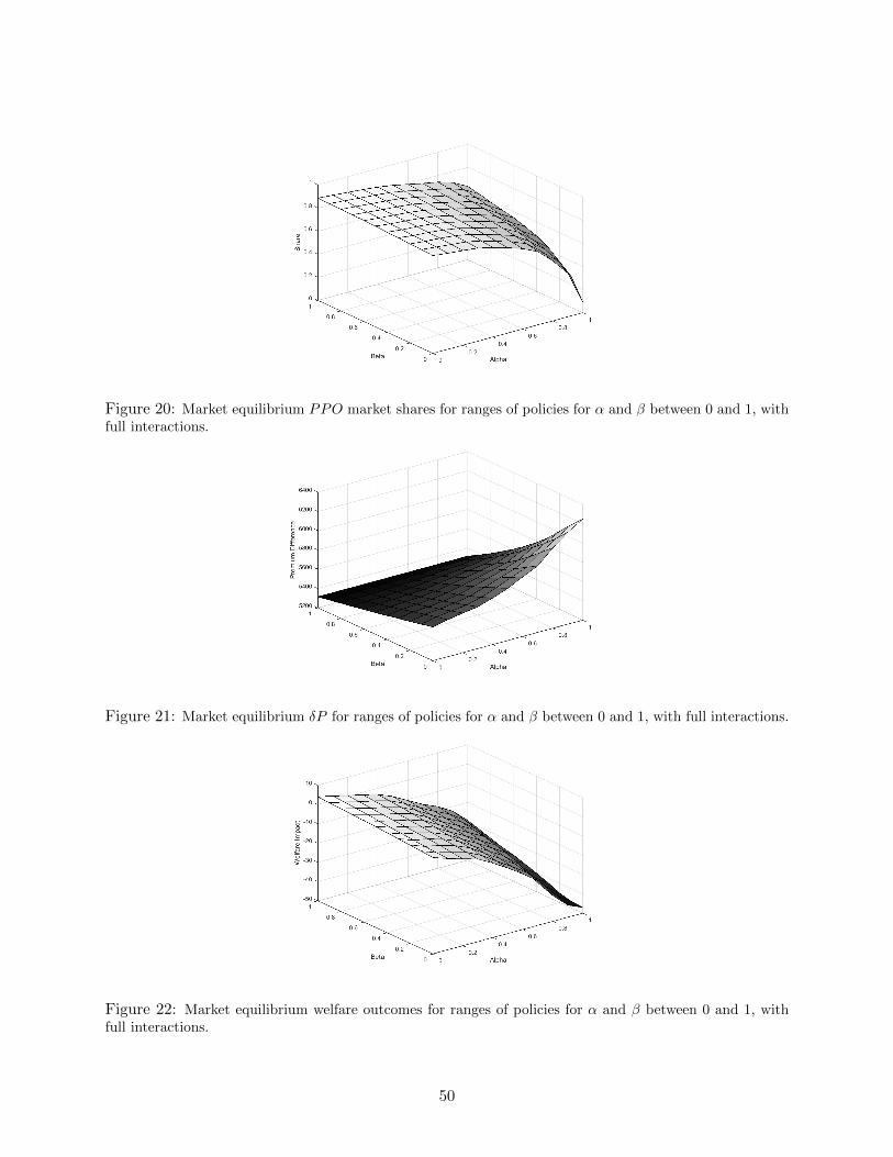
Figure 20: Market equilibrium PPO market shares for ranges of policies for α and β between 0 and 1, withfull interactions.

Figure 21: Market equilibrium δP for ranges of policies for α and β between 0 and 1, with full interactions.

Figure 22: Market equilibrium welfare outcomes for ranges of policies for α and β between 0 and 1, withfull interactions.

50

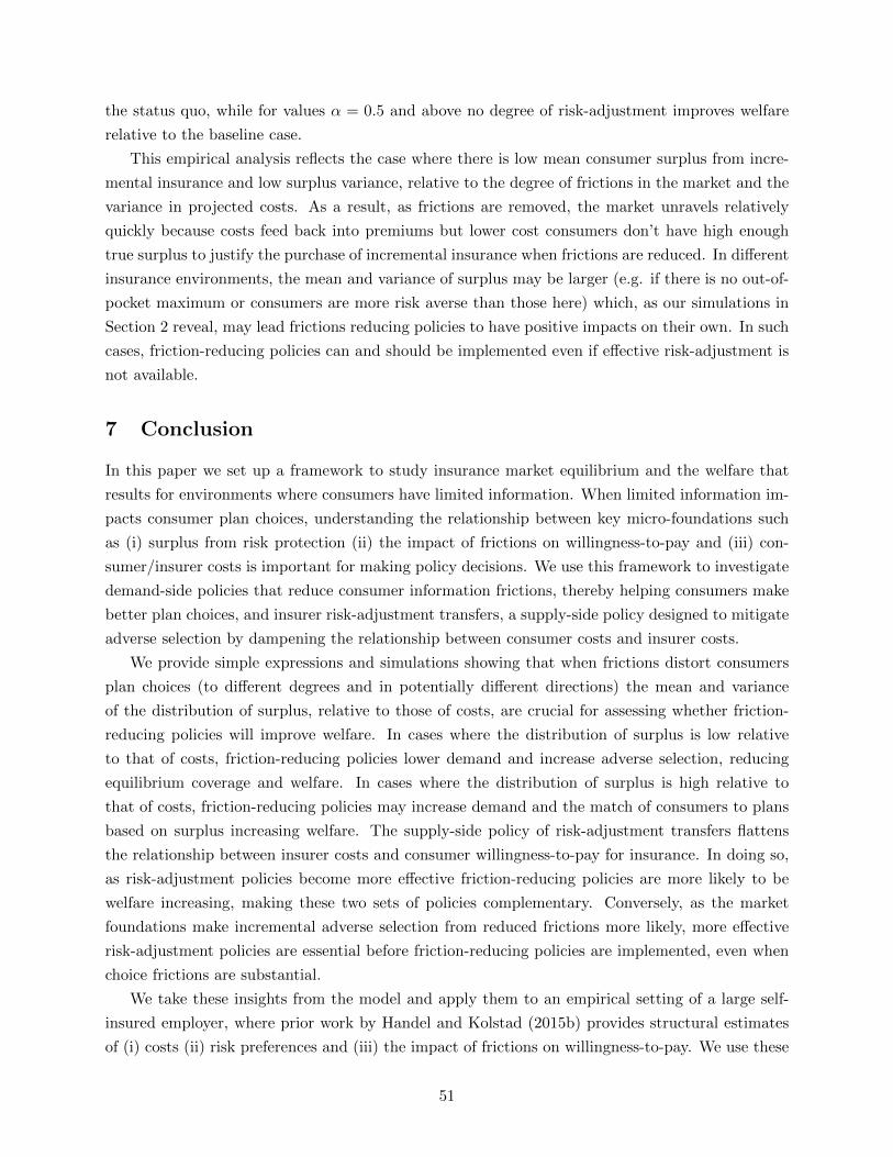
the status quo, while for values α = 0.5 and above no degree of risk-adjustment improves welfare

relative to the baseline case.

This empirical analysis reflects the case where there is low mean consumer surplus from incre-

mental insurance and low surplus variance, relative to the degree of frictions in the market and the

variance in projected costs. As a result, as frictions are removed, the market unravels relatively

quickly because costs feed back into premiums but lower cost consumers don’t have high enough

true surplus to justify the purchase of incremental insurance when frictions are reduced. In different

insurance environments, the mean and variance of surplus may be larger (e.g. if there is no out-of-

pocket maximum or consumers are more risk averse than those here) which, as our simulations in

Section 2 reveal, may lead frictions reducing policies to have positive impacts on their own. In such

cases, friction-reducing policies can and should be implemented even if effective risk-adjustment is

not available.

7 Conclusion

In this paper we set up a framework to study insurance market equilibrium and the welfare that

results for environments where consumers have limited information. When limited information im-

pacts consumer plan choices, understanding the relationship between key micro-foundations such

as (i) surplus from risk protection (ii) the impact of frictions on willingness-to-pay and (iii) con-

sumer/insurer costs is important for making policy decisions. We use this framework to investigate

demand-side policies that reduce consumer information frictions, thereby helping consumers make

better plan choices, and insurer risk-adjustment transfers, a supply-side policy designed to mitigate

adverse selection by dampening the relationship between consumer costs and insurer costs.

We provide simple expressions and simulations showing that when frictions distort consumers

plan choices (to different degrees and in potentially different directions) the mean and variance

of the distribution of surplus, relative to those of costs, are crucial for assessing whether friction-

reducing policies will improve welfare. In cases where the distribution of surplus is low relative

to that of costs, friction-reducing policies lower demand and increase adverse selection, reducing

equilibrium coverage and welfare. In cases where the distribution of surplus is high relative to

that of costs, friction-reducing policies may increase demand and the match of consumers to plans

based on surplus increasing welfare. The supply-side policy of risk-adjustment transfers flattens

the relationship between insurer costs and consumer willingness-to-pay for insurance. In doing so,

as risk-adjustment policies become more effective friction-reducing policies are more likely to be

welfare increasing, making these two sets of policies complementary. Conversely, as the market

foundations make incremental adverse selection from reduced frictions more likely, more effective

risk-adjustment policies are essential before friction-reducing policies are implemented, even when

choice frictions are substantial.

We take these insights from the model and apply them to an empirical setting of a large self-

insured employer, where prior work by Handel and Kolstad (2015b) provides structural estimates

of (i) costs (ii) risk preferences and (iii) the impact of frictions on willingness-to-pay. We use these

51

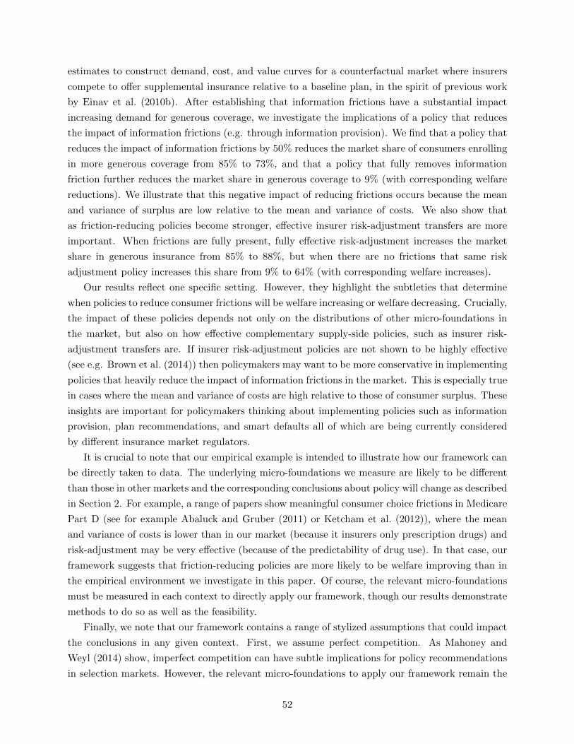
estimates to construct demand, cost, and value curves for a counterfactual market where insurers

compete to offer supplemental insurance relative to a baseline plan, in the spirit of previous work

by Einav et al. (2010b). After establishing that information frictions have a substantial impact

increasing demand for generous coverage, we investigate the implications of a policy that reduces

the impact of information frictions (e.g. through information provision). We find that a policy that

reduces the impact of information frictions by 50% reduces the market share of consumers enrolling

in more generous coverage from 85% to 73%, and that a policy that fully removes information

friction further reduces the market share in generous coverage to 9% (with corresponding welfare

reductions). We illustrate that this negative impact of reducing frictions occurs because the mean

and variance of surplus are low relative to the mean and variance of costs. We also show that

as friction-reducing policies become stronger, effective insurer risk-adjustment transfers are more

important. When frictions are fully present, fully effective risk-adjustment increases the market

share in generous insurance from 85% to 88%, but when there are no frictions that same risk

adjustment policy increases this share from 9% to 64% (with corresponding welfare increases).

Our results reflect one specific setting. However, they highlight the subtleties that determine

when policies to reduce consumer frictions will be welfare increasing or welfare decreasing. Crucially,

the impact of these policies depends not only on the distributions of other micro-foundations in

the market, but also on how effective complementary supply-side policies, such as insurer risk-

adjustment transfers are. If insurer risk-adjustment policies are not shown to be highly effective

(see e.g. Brown et al. (2014)) then policymakers may want to be more conservative in implementing

policies that heavily reduce the impact of information frictions in the market. This is especially true

in cases where the mean and variance of costs are high relative to those of consumer surplus. These

insights are important for policymakers thinking about implementing policies such as information

provision, plan recommendations, and smart defaults all of which are being currently considered

by different insurance market regulators.

It is crucial to note that our empirical example is intended to illustrate how our framework can

be directly taken to data. The underlying micro-foundations we measure are likely to be different

than those in other markets and the corresponding conclusions about policy will change as described

in Section 2. For example, a range of papers show meaningful consumer choice frictions in Medicare

Part D (see for example Abaluck and Gruber (2011) or Ketcham et al. (2012)), where the mean

and variance of costs is lower than in our market (because it insurers only prescription drugs) and

risk-adjustment may be very effective (because of the predictability of drug use). In that case, our

framework suggests that friction-reducing policies are more likely to be welfare improving than in

the empirical environment we investigate in this paper. Of course, the relevant micro-foundations

must be measured in each context to directly apply our framework, though our results demonstrate

methods to do so as well as the feasibility.

Finally, we note that our framework contains a range of stylized assumptions that could impact

the conclusions in any given context. First, we assume perfect competition. As Mahoney and

Weyl (2014) show, imperfect competition can have subtle implications for policy recommendations

in selection markets. However, the relevant micro-foundations to apply our framework remain the

52

same. Second, our approach maintains quite stylized assumptions about the potentially endogenous

relationship between the extent of competition in the market and consumer information. It is

possible that the extent of limited information in any given setting is partially related to the degree

of competition and/or the extent of risk-adjustment policies, an area that we believe is an interesting

topic for future work. Third, we abstracted away from consumer moral hazard, to clearly focus on

the other micro-foundations in the market. Though the relationships we explore would generally be

robust to including moral hazard in the model, the mean and variance of that price sensitivity could

have important implications for whether increasing coverage is a desirable social goal. We believe

that extending our analysis by relaxing these assumptions is an interesting avenue for future work.

Fourth, we focus on the case where frictions push consumers towards more generous coverage: this

example is relevant in practice, and much of the intuition of our framework can be applied to that

case, in reverse, where relevant in future work.

53

References

Abaluck, J. and J. Gruber, “Choice Inconsistencies Among the Elderly: Evidence from PlanChoice in the Medicare Part D Program,” American Economic Review, 2011, 101 (4), 1180–1210.

Akerlof, G., “The Market for ‘Lemons’: Quality Uncertainty and the Market Mechanism,” Quar-terly Journal of Economics, 1970, 84 (3), 488–500.

Alcott, H. and D. Taubinsky, “Evaluating Behaviorally-Motivated Polcy: Evidence from theLightbulb Market,” The American Economic Review, 2015, 105 (8), 2501–2538.

Azevedo, E. and D. Gottlieb, “Perfect Competition in Markets with Adverse Selection,” May2015. University of Pennsylvania Working Paper.

Baicker, K., S. Mullainathan, and J. Schwartzstein, “Behavioral Hazard in Health Insur-ance,” May 2015. Harvard Working Paper.

Barseghyan, L., F. Molinari, T. O’Donoghue, and J. Teitelbaum, “The Nature of RiskPreferences: Evidence from Insurance Choices,” American Economic Review, 2013, 103 (6),2499–2529.

Bernheim, D., A. Fradkin, and I. Popov, “The Welfare Economics of Default Options in401(k) Plans,” The Quarterly Journal of Economics, forthcoming.

Bertrand, M., E. Duflo, and S. Mullainathan, “How Much Should We Trust Differences-In-Differences Estimates?,” Quarterly Journal of Economics, 2004, 119 (1), 249–275.

Bhargava, S., G. Loewenstein, and J. Sydnor, “Do Individuals Make Sensible Health Insur-ance Decisions? Evidence From a Menu with Dominated Options,” April 2015. Carnegie Mellonworking paper.

Bronnenberg, Bart J., Jean-Pierre Dube, Matthew Gentzkow, and Jesse M. Shapiro,“Do Pharmacists Buy Bayer? Informed Shoppers and the Brand Premium,” August 2014. Uni-versity of Chicago Working Paper.

Brot-Goldberg, Z., A. Chandra, B. Handel, and J. Kolstad, “What Does a DeductibleDo? The Impact of Cost-Sharing on Health Care Prices, Quantities, and Spending Dynamics,”October 2015. NBER working paper no. 21632.

Brown, J., M. Duggan, I. Kuziemko, and W. Woolston, “How Does Risk Selection Respondto Risk Adjustment? Evidence From The Medicare Advantage Program,” American EconomicReview, 2014, 104 (10), 3335–3364.

Bundorf, Kate, Jonathan Levin, and Neale Mahoney, “Pricing and Welfare in Health PlanChoice,” American Economic Review, 2012, 102 (7), 3214–3248.

Cohen, A. and L. Einav, “Estimating Risk Preferences from Deductible Choice,” The AmericanEconomic Review, 2007, 97 (3), 745–788.

Cutler, D. and S. Reber, “Paying for Health Insurance: The Tradeoff Between Competitionand Adverse Selection,” Quarterly Journal of Economics, 1998, 113 (2), 433–466.

Dixit, A. and V. Norman, “Advertising and Welfare,” The Bell Journal of Economics, 1978, 9(1), 1–17.

54

Einav, L., A. Finkelstein, and J. Levin, “Beyond Testing: Empirical Models of InsuranceMarkets,” Annual Review of Economics, 2010, 2, 311–336.

, , and M. Cullen, “Estimating Welfare in Insurance Markets Using Variation in Prices,”Quarterly Journal of Economics, 2010, 125 (3), 877–921.

Geruso, M. and T. McGuire, “Tradeoffs in the Design of Health Plan Payment Systems: Fit,Power, and Balance,” July 2014. University of Texas Working Paper.

Glazer, J., T. McGuire, and J. Shi, “Risk Adjustment of Health Plan Payments to CorrectInefficient Plan Choice from Adverse Selection,” March 2014. NBER Working Paper No. 19998.

Hackmann, M., J. Kolstad, and A. Kowalski, “Adverse Selection and an Individual Mandate:When Theory Meets Practice,” American Economic Review, 2015, 105 (3), 1030–1060.

Handel, B., “Adverse Selection and Inertia in Health Insurance Markets: When Nudging Hurts,”American Economic Review, 2013, 103 (7), 2643–2682.

and J. Kolstad, “Getting the Most from Marketplaces: Smart Policies on Health InsuranceChoice,” Hamilton Project Discussion Paper, 2015, (8).

and , “Health Insurance For Humans: Information Frictions, Plan Choice, and ConsumerWelfare,” American Economic Review, 2015, 105 (8), 2449–2500.

, I. Hendel, and M. Whinston, “Equilibria in Health Exchanges: Adverse Selection vs.Reclassification Risk,” Econometrica, 2015, 83 (4), 1261–1313.

Kaiser Family Foundation, “Focus on Health Reform: Summary of the Affordable Care Act,”http://kaiserfamilyfoundation.files.worldpress.com/2011/04/8061-021.pdf 2011.

Ketcham, J., C. Lucarelli, E. Miravete, and C. Roebuck, “Sinking, Swimming, or Learningto Swim in Medicare Part D?,” The American Economic Review, 2012, 102 (6), 2639–2673.

Kling, Jeffrey, Sendhil Mullainathan, Eldar Shafir, Lee Vermeulen, and Marian Wro-bel, “Comparison Friction: Experimental Evidence from Medicare Drug Plans,” Quarterly Jour-nal of Economics, 2012, 127 (1), 199–235.

Mahoney, N. and G. Weyl, “Imperfect Competition in Selection Markets,” September 2014.University of Chicago Working Paper.

Manski, C. and S. Lerman, “The Estimation of Choice Probabilities from Choice Based Sam-ples,” Econometrica, 1977, 45 (8), 1977–1988.

Polyakova, M., “Regulation of Insurance with Adverse Selection and Switching Costs: Evidencefrom Medicare Part D,” January 2015. Stanford University working paper.

Rothschild, M. and J. Stiglitz, “Equilibrium in Competitive Insurance Markets: An Essay onthe Economics of Imperfect Information,” Quarterly Journal of Economics, 1976, 90, 630–649.

Solon, G., S. Haider, and J. Wooldridge, “What Are We Weighting For?,” February 2013.NBER Working Paper no. 18859.

Spinnewijn, J., “Heterogeneity, Demand for Insurance and Adverse Selection,” September 2015.LSE working paper.

55

Taubinsky, D., “Attention Variation and Welfare: Theory and Evidence from a Tax SalienceExperiment,” January 2016. Harvard University Working Paper.

Train, K., Discrete Choice Methods with Simulation, 2nd ed., Cambridge University Press, 2009.

Veiga, A. and G. Weyl, “Product Design in Selection Markets,” January 2015. University ofChicago Working Paper.

Weyl, G. and A. Veiga, “Pricing Institutions and the Welfare Cost of Adverse Selection,”October 2015. University of Chicago Working Paper.

56

A Appendix: Proofs

Proof of Proposition 1: We consider a budget-balanced policy x that maintains the ordering ofindividuals’ willingness-to-pay and thus the corresponding surplus from buying insurance conditionalon the share of insured individuals. We denote by wi (x) individual i′s net willingness-to-pay and thecorresponding density by gw(x). Equilibrium welfare for policy x (not accounting for the budgetarycost) equals

W (x) =

∫D−1(Q(x);x)

Ew′ (s) gw(x)

(w′)dw′,

=

∫D−1(Q(x);0)

Ew′ (s) g(w′)dw′.

The second equality follows by maintaining the ordering for any intensity of the policy x. Thewelfare effect of an increase in x only goes through the equilibrium quantity,

W ′ (x) =∂

∂Q

[∫ ∞D−1(Q(x);x)

Ew′ (s) gw(x)

(w′)dw′

]Q′ (x) .

Using Leibniz’ rule and ∂∂QD

−1 = −1gw(x) , we find

W ′ (x) = −EP (x) (s) gw(x) (P )∂

∂QD−1 (Q (x) ;x)Q′ (x)

= EP (x) (s)Q′ (x) =[P (x)− EP (x) (c)− EP (x) (f)

]Q′ (x) .

Hence, a policy that increases Q, ceteris paribus, increases welfare if and only if P − EP (c) ≥EP (f).

Proof of Proposition 2: The equilibrium is characterized by P c (α) = E≥P c(α) (c) where P c (α) =D−1 (Qc (α) ;α). We can solve for the change in coverage by implicit differentiation. The mainchallenge is to derive how the conditional expectation E≥P c (c) changes.We first consider a change in the equilibrium price. Note that

E≥P c (c) =1

1−Gw(α) (P c)

∫ ∞P c

Ew(α)=w′ (c) gw(α)

(w′)dw′,

where we denote individual i′s net willingness-to-pay by wi (α) and the corresponding density bygw(α). Using Leibniz’ rule, we find

∂

∂P

[∫P cEw(α)=w′ (c) g

w(α)(w′)dw′]

= −Ew(α)=P c (c) gw(α) (P c) .

Hence, using ∂[1−Gw(α) (P )

]/∂P = −gw(α) (P ), we find

∂

∂PE≥P c (c) = [E≥P c (c)− EP c (c)]

gw(α) (P c)

1−Gw(α) (P c),

which depends on the difference between average and marginal cost.Evaluating the impact of the information policy on E≥P c (c) is more difficult, since it interacts with

57

individuals’ friction value. However, using the law of iterated expectations, we can re-write∫P cEw(α)=w′ (c) g

w(α)(w′)dw′

=

∫ ∫P cE(c|w (α) = w′, f = f ′

)gw(α)|f (w′|f ′) dw′gf (f ′) df ′

=

∫ ∫P cE(c|w = w′ + αf ′, f = f ′

)gw|f

(w′ + αf ′|f ′

)dw′gf

(f ′)df ′

=

∫ ∫P c+αf ′

E(c|w = w′, f = f ′

)gw|f

(w′|f ′

)dw′gf

(f ′)df ′.

The last equality uses the substitution w′ = w′ + αf ′ and thus dw′ = dw′. Now we can write

∂

∂α


w(α)(w′)dw′]

=

∫∂

∂α

[∫P c+αf

E(c|w = w′, f = f ′

)gw|f

(w′|f ′

)dw′]gf(f ′)df ′

= −∫ [

E(c|w = P c + αf ′, f = f ′

)gw|f

(P c + αf ′|f ′

)× f ′

]gf(f ′)df ′

= −∫ [

E(c× f |w = P c + αf ′, f = f ′

)gw|f

(P c + αf ′|f ′

)]gf(f ′)df ′.

Using again the law of iterated expectations and the reverse subsitution, we find

∂

∂α


w(α)(w′)dw′]

= −EP c (c× f) gw(α) (P c) .

In an analogue way, we can find

∂

∂α

[∫P cgw(α)

(w′)dw′]

= −EP c (f) gw(α) (P c) .

Hence,

∂

∂αE≥P c (c) =

[E≥P c (c)Ew(α) (f)− EP c (c× f)

] gw(α) (P c)

1−Gw(α) (P c)

=[(E≥P c (c)− EP c (c))Ew(α) (f)− covP c (c, f)

] gw(α) (P c)

1−Gw(α) (P c),

which depends on the difference between average and marginal costs as well.By implicit differentiation of the equilibrium condition D−1 (Qc (α) ;α) = E≥D−1(Qc(α);α) (c), we

find

Qc′ (α) = −[1− ∂

∂P cE≥P c (c)] ∂D−1(Qc;α)

∂α − ∂∂αE≥P c (c)[

1− ∂∂P cE≥P c (c)

] ∂D−1(Qc;α)∂Q

.

with ∂D−1(Qc;α)∂Q = 1

−gw(α)(P c)and ∂D−1(Qc;α)

∂α = −EP c (f). Putting things together, the terms with

58

[E≥P c (c)− EP c (c)] drop out of the numerator and we find

Qc′ (α) = −EP c (f)− covP c (c, f) |εD(P c)|

P c

1− [E≥P c (c)− EP c (c)] |εD(P c)|P c

gw(α) (P c) ,

using gw(α)(P c)

1−Gw(α)(P c)= |εD(P c)|

P c . Notice that for a uniform subsidy S such that P c = E≥P c (c) +S, we

have

Qc′ (S) =1

1− [E≥P c (c)− EP c (c)] |εD(P c)|P c

gw(α) (P c) ≡ ηc.

Hence, the Proposition follows.

Proof of Proposition 3: Consider the equilibrium price P (α) and quantity Q (α). Welfare equals

W (α) =

∫P (α)

Ew(α)=w′ (s) gw(α)

(w′)dw′,

where P (α) = D−1 (Q (α) , α). The total impact of the policy on welfare depends on the policy’seffect on the equilibrium quantity and its direct effect on welfare,

W ′ (α) =∂W∂P

∂D−1 (Q (α) , α)

∂QQ′ (α) +

∂W∂P

∂D−1 (Q (α) , α)

∂α+∂W∂α

.

By analogy to the proof of Proposition 2, we find

∂W∂P

= −EP (α) (s) gw(α) (P (α))

∂W∂α

= −EP (α) (s× f) gw(α) (P (α)) .

Using ∂D−1(Q(α);α)∂Q = 1

−gw(α)(P (α))and ∂D−1(Q(α);α)

∂α = −EP (α) (f), we find

W ′ (α) = EP (α) (s)Q′ (α) + EP (α) (s)EP (α) (f) gw(α) (P (α))− EP (α) (s× f) gw(α) (P (α))

= EP (α) (s)Q′ (α)− covP (α) (s, f) gw(α) (P (α))

and the proposition immediately follows.

Proof of Proposition 4 For a risk-adjustment policy β the competitive equilibrium is determinedby

P c (β) = E≥P c(β) (c (β))

and Qc (β) = D−1 (P c (β)). By implicit differentiation, we find

Qc′ (β) = −− ∂∂βE≥P c (c (β))[

1− ∂∂P cE≥P c (c (β))

] ∂D−1(Qc;β)∂Q

.

Like in the proof of Proposition 1, we find ∂D−1(Qc;β)∂Q = 1

−g(P c) and

∂

∂P cE≥P c (c (β)) = [E≥P c (c (β))− EP c (c (β))]

g (P c)

1−G (P c).

59

Moreover,

∂

∂βE≥P c (c (β)) =

∂

∂β

[1

1−G (P c)

∫ ∞P c

Ew′ (c (β)) g(w′)dw′]

=1

1−G (P c)

∫ ∞P c

Ew′ (− [c− Ec]) g(w′)dw′

= E≥P c (c)− Ec

Hence,

Qc′ (β) =E≥P c (c)− Ec

1− [E≥P c (c)− EP c (c)] |εD(P c)|P c

g (P c)

= ηc × [E≥P c (c)− Ec] ,

where ηc equals the equilibrium impact of a uniform subsidy.Welfare equals

W (β) =

∫D−1(Qc(β))

Ew (s) g(w′)dw′.

Hence,

W ′ (β) = −EP c (s)1

−g (P c)g (P c)Qc′ (β) .

This proves the second expression of the Proposition.

60

B Appendix: Cost Model Setup and Estimation

This appendix describes the details of the cost model, which is summarized at a high-level insection 4.58 The output of this model, Fkjt, is a family-plan-time specific distribution of predictedout-of-pocket expenditures for the upcoming year. This distribution is an important input into thechoice model, where it enters as a family’s predictions of its out-of-pocket expenses at the time ofplan choice, for each plan option.59 We predict this distribution in a sophisticated manner thatincorporates (i) past diagnostic information (ICD-9 codes) (ii) the Johns Hopkins ACG predictivemedical software package (iii) a non-parametric model linking modeled health risk to total medicalexpenditures using observed cost data and (iv) a detailed division of medical claims and health plancharacteristics to precisely map total medical expenditures to out-of-pocket expenses.The level ofprecision we gain from the cost model leads to more credible estimates of the choice parameters ofprimary interest (e.g. risk preferences and information friction impacts).

In order to most precisely predict expenses, we categorize the universe of total medical claimsinto four mutually exclusive and exhaustive subdivisions of claims using the claims data. Thesecategories are (i) hospital and physician (ii) pharmacy (iii) mental health and (iv) physician officevisit. We divide claims into these four specific categories so that we can accurately characterize theplan-specific mappings from total claims to out-of-pocket expenditures since each of these categoriesmaps to out-of-pocket expenditures in a different manner. We denote this four dimensional vectorof claims Cit and any given element of that vector Cd,it where d ∈ D represents one of the fourcategories and i denotes an individual (employee or dependent). After describing how we predictthis vector of claims for a given individual, we return to the question of how we determine out-of-pocket expenditures in plan j given Cit.

Denote an individual’s past year of medical diagnoses and payments by ξit and the demographicsage and sex by ζit. We use the ACG software mapping, denoted A, to map these characteristicsinto a predicted mean level of health expenditures for the upcoming year, denoted θ:

A : ξ × ζ → θ

In addition to forecasting a mean level of total expenditures, the software has an applicationthat predicts future mean pharmacy expenditures. This mapping is analogous to A and outputs aprediction λ for future pharmacy expenses.

We use the predictions θ and λ to categorize similar groups of individuals across each of fourclaims categories in vector in Cit. Then for each group of individuals in each claims category, weuse the actual ex post realized claims for that group to estimate the ex ante distribution for eachindividual under the assumption that this distribution is identical for all individuals within the cell.Individuals are categorized into cells based on different metrics for each of the four elements of C:

Pharmacy: λit

Hospital / Physician (Non-OV): θit

Physician Office Visit: θit

Mental Health: CMH,i,t−1

For pharmacy claims, individuals are grouped into cells based on the predicted future mean phar-

58The model is similar to that used in Handel (2013).59In the consumer choice model, this is mostly useful for estimating out-of-pocket expenditures in the HDHP, since

the PPO plan has essentially zero expenditures.

61

macy claims measure output by the ACG software, λit. For the categories of hospital / physician(non office visit) and physician office visit claims individuals are grouped based on their mean pre-dicted total future health expenses, θit. Finally, for mental health claims, individuals are groupedinto categories based on their mental health claims from the previous year, CMH,i,t−1 since (i)mental health claims are very persistent over time in the data and (ii) mental health claims areuncorrelated with other health expenditures in the data. For each category we group individualsinto a number of cells between 8 and 12, taking into account the trade off between cell size andprecision.

Denote an arbitrary cell within a given category d by z. Denote the population in a givencategory-cell combination (d, z) by Idz. Denote the empirical distribution of ex-post claims in

this category for this population ˆGIdz(·). Then we assume that each individual in this cell has a

distribution equal to a continuous fit of ˆGIdz(·), which we denote Gdz:

$ : ˆGIdz(·)→ Gdz

We model this distribution continuously in order to easily incorporate correlations across d. Oth-erwise, it would be appropriate to use GIdz as the distribution for each cell.

The above process generates a distribution of claims for each d and z but does not modelcorrelations over D. It is important to model correlation over claim categories because it is likelythat someone with a bad expenditure shock in one category (e.g. hospital) will have high expenses inanother area (e.g. pharmacy). We model correlation at the individual level by combining marginaldistributions Gidt ∀ d with empirical data on the rank correlations between pairs (d, d′).60 Here,Gidt is the distribution Gdz where i ∈ Idz at time t. Since correlations are modeled across d we pickthe metric θ to group people into cells for the basis of determining correlations (we use the samecells that we use to determine group people for hospital and physician office visit claims). Denotethese cells based on θ by zθ. Then for each cell zθ denote the empirical rank correlation betweenclaims of type d and type d′ by ρzθ(d, d

′). Then, for a given individual i we determine the jointdistribution of claims across D for year t, denoted Hit(·), by combining i’s marginal distributionsfor all d at t using ρzθ(d, d

′):

Ψ : GiDt × ρzθit (D,D′)→ Hit

Here, GiDt refers to the set of marginal distributions Gidt∀d ∈ D and ρzθit (D,D′) is the set of

all pairwise correlations ρzθit (d, d′)∀(d, d′) ∈ D2. In estimation we perform Ψ by using a Gaussian

copula to combine the marginal distribution with the rank correlations, a process which we describemomentarily.

The final part of the cost model maps the joint distribution Hit of the vector of total claimsC over the four categories into a distribution of out of pocket expenditures for each plan. For theHDHP we construct a mapping from the vector of claims C to out of pocket expenditures OOPj :

Ωj : C → OOPj

This mapping takes a given draw of claims from Hit and converts it into the out of pocket expendi-tures an individual would have for those claims in plan j. This mapping accounts for plan-specificfeatures such as the deductible, co-insurance, co-payments, and out of pocket maximums listed intable A-2. We test the mapping Ωj on the actual realizations of the claims vector C to verify thatour mapping comes close to reconstructing the true mapping. Our mapping is necessarily simpler

60It is important to use rank correlations here to properly combine these marginal distribution into a joint distri-bution. Linear correlation would not translate empirical correlations to this joint distribution appropriately.

62

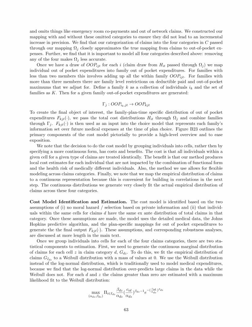
and omits things like emergency room co-payments and out of network claims. We constructed ourmapping with and without these omitted categories to ensure they did not lead to an incrementalincrease in precision. We find that our categorization of claims into the four categories in C passedthrough our mapping Ωj closely approximates the true mapping from claims to out-of-pocket ex-penses. Further, we find that it is important to model all four categories described above: removingany of the four makes Ωj less accurate.

Once we have a draw of OOPijt for each i (claim draw from Hit passed through Ωj) we mapindividual out of pocket expenditures into family out of pocket expenditures. For families withless than two members this involves adding up all the within family OOPijt. For families withmore than three members there are family level restrictions on deductible paid and out-of-pocketmaximums that we adjust for. Define a family k as a collection of individuals ik and the set offamilies as K. Then for a given family out-of-pocket expenditures are generated:

Γj : OOPik,jt → OOPkjt

To create the final object of interest, the family-plan-time specific distribution of out of pocketexpenditures Fkjt(·), we pass the total cost distributions Hit through Ωj and combine familiesthrough Γj . Fkjt(·) is then used as an input into the choice model that represents each family’sinformation set over future medical expenses at the time of plan choice. Figure B23 outlines theprimary components of the cost model pictorially to provide a high-level overview and to easeexposition.

We note that the decision to do the cost model by grouping individuals into cells, rather then byspecifying a more continuous form, has costs and benefits. The cost is that all individuals within agiven cell for a given type of claims are treated identically. The benefit is that our method produceslocal cost estimates for each individual that are not impacted by the combination of functional formand the health risk of medically different individuals. Also, the method we use allows for flexiblemodeling across claims categories. Finally, we note that we map the empirical distribution of claimsto a continuous representation because this is convenient for building in correlations in the nextstep. The continuous distributions we generate very closely fit the actual empirical distribution ofclaims across these four categories.

Cost Model Identification and Estimation. The cost model is identified based on the twoassumptions of (i) no moral hazard / selection based on private information and (ii) that individ-uals within the same cells for claims d have the same ex ante distribution of total claims in thatcategory. Once these assumptions are made, the model uses the detailed medical data, the JohnsHopkins predictive algorithm, and the plan-specific mappings for out of pocket expenditures togenerate the the final output Fkjt(·). These assumptions, and corresponding robustness analyses,are discussed at more length in the main text.

Once we group individuals into cells for each of the four claims categories, there are two sta-tistical components to estimation. First, we need to generate the continuous marginal distributionof claims for each cell z in claim category d, Gdz. To do this, we fit the empirical distribution ofclaims GIdz to a Weibull distribution with a mass of values at 0. We use the Weibull distributioninstead of the log-normal distribution, which is traditionally used to model medical expenditures,because we find that the log-normal distribution over-predicts large claims in the data while theWeibull does not. For each d and z the claims greater than zero are estimated with a maximumlikelihood fit to the Weibull distribution:

max(αdz ,βdz)

Πi∈Idzβdzαdz

(cidαdz

)βdz−1e−(

cidαdz

)βdz

63

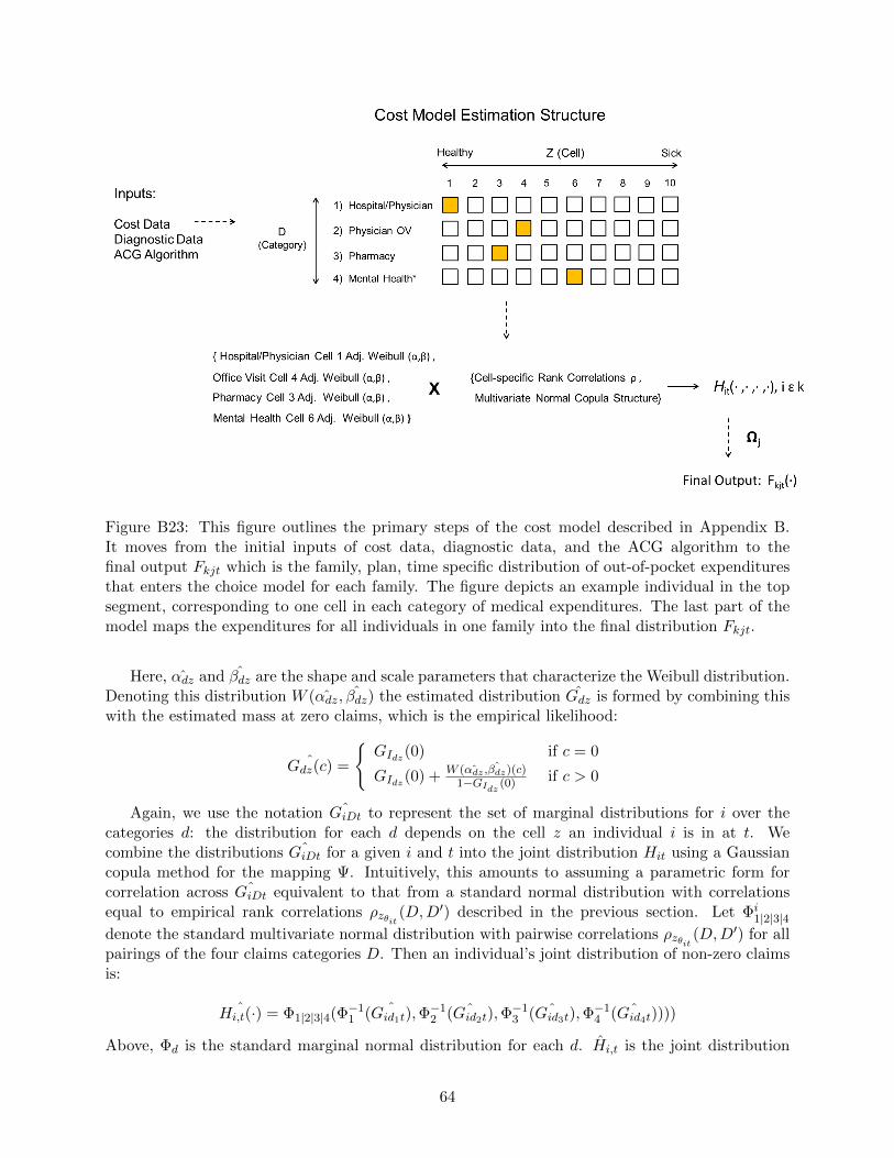
Figure B23: This figure outlines the primary steps of the cost model described in Appendix B.It moves from the initial inputs of cost data, diagnostic data, and the ACG algorithm to thefinal output Fkjt which is the family, plan, time specific distribution of out-of-pocket expendituresthat enters the choice model for each family. The figure depicts an example individual in the topsegment, corresponding to one cell in each category of medical expenditures. The last part of themodel maps the expenditures for all individuals in one family into the final distribution Fkjt.

Here, αdz and βdz are the shape and scale parameters that characterize the Weibull distribution.Denoting this distribution W (αdz, βdz) the estimated distribution Gdz is formed by combining thiswith the estimated mass at zero claims, which is the empirical likelihood:

ˆGdz(c) =

GIdz(0) if c = 0

GIdz(0) + W ( ˆαdz , ˆβdz)(c)1−GIdz (0) if c > 0

Again, we use the notation ˆGiDt to represent the set of marginal distributions for i over thecategories d: the distribution for each d depends on the cell z an individual i is in at t. Wecombine the distributions ˆGiDt for a given i and t into the joint distribution Hit using a Gaussiancopula method for the mapping Ψ. Intuitively, this amounts to assuming a parametric form forcorrelation across ˆGiDt equivalent to that from a standard normal distribution with correlationsequal to empirical rank correlations ρzθit (D,D

′) described in the previous section. Let Φi1|2|3|4

denote the standard multivariate normal distribution with pairwise correlations ρzθit (D,D′) for all

pairings of the four claims categories D. Then an individual’s joint distribution of non-zero claimsis:

ˆHi,t(·) = Φ1|2|3|4(Φ−11 ( ˆGid1t),Φ

−12 ( ˆGid2t),Φ

−13 ( ˆGid3t),Φ

−14 ( ˆGid4t))))

Above, Φd is the standard marginal normal distribution for each d. Hi,t is the joint distribution

64

of claims across the four claims categories for each individual in each time period. After this isestimated, we determine our final object of interest Fkjt(·) by simulating K multivariate draws

from Hi,t for each i and t, and passing these values through the plan-specific total claims to out ofpocket mapping Ωj and the individual to family out of pocket mapping Γj . The simulated Fkjt(·)for each k, j, and t is then used as an input into estimation of the choice model.

New Employees. For the first-stage full population model that compares new employees toexisting employees to identify the extent of inertia, we need to estimate Fkj for new families. Un-like for existing families, we don’t observe past medical diagnoses / claims for these families, wejust observe these things after they join the firm and after they have made their first health planchoice with the firm. We deal with this issue with a simple process that creates an expected ex antehealth status measure. We backdate health status in a Bayesian manner: if a consumer has healthstatus x ex post we construct ex ante health status y as an empirical mixture distribution f(y|x).f(y|x) is estimated empirically and can be thought of as a reverse transition probability (if you arex in period 2, what is the probability you were y in period 1?). Then, for each possible ex ante y,we use the distributions of out-of-pocket expenditures F estimated from the cost model for thattype. Thus, the actual distribution used for such employees is described by

∫x∈X f(y|x)F (y)dy.

The actual cost model estimates F (y) do not include new employees and leverages actual claimsdata for employees who have a past observed year of this data.

65

C Appendix: Choice Model Identification and Estimation

This appendix describes the algorithm by which we estimate the parameters of the choice model.The corresponding section in the text provided a high-level overview of this algorithm and out-lined the estimation assumptions we make regarding choice model fundamentals and their links toobservable data.

We estimate the choice model using a random coefficients probit simulated maximum likelihoodapproach similar to that summarized in Train (2009) and to that used in Handel (2013). Thesimulated maximum likelihood estimation approach has the minimum variance for a consistentand asymptotically normal estimator, while not being too computationally burdensome in ourframework. We set up a likelihood function to predict the health choices of consumers in t4. Themaximum likelihood estimator selects the parameter values that maximize the similarity betweenactual choices and choices simulated with the parameters.

First, the estimator simulates Q draws for each family from the distribution of health expen-ditures output from the cost model, Fk for each family. The estimator also simulates D draws foreach family-year from the distribution of the random coefficient γk, as well as from the distributionof idiosyncratic preference shocks εkj .

We define θ as the full set of model parameters of interest for the full / primary specificationin Section 4:61

θ ≡ (µγ , δ, σγ , σε, η1, η0, β).

We denote θdk as one draw derived from these parameters for each family, including the param-eters that are constant across draws (e.g., for observable heterogeneity in γ or η) and those whichchange with each draw (unobservable heterogeneity in γ and ε):62

θdk ≡ (γk, εkJ , ηk, β)

Denote θDk as the set of all D simulated parameter draws for family k. For each θdk ∈ θDk, theestimator uses all Q health draws to compute family-plan-specific expected utilities Udkj followingthe choice model outlined earlier in section 4. Given these expected utilities for each θdk, wesimulate the probability of choosing plan j∗ in each period using a smoothed accept-reject functionwith the form:

Prdk(j = j∗) =

(1

−Udkj∗(·)

ΣJ1

−Uskj(·))τ

Σj(

1−U

skj(·)

ΣJ1

−Uskj(·))τ

This smoothed accept-reject methodology follows that outlined in Train (2009) with some slightmodifications to account for the expected utility specification. In theory, conditional on θdk, wewould want to pick the j that maximizes Ukj for each family, and then average over D to getfinal choice probabilities. However, doing this leads to a likelihood function with flat regions,because for small changes in the estimated parameters θ, the discrete choice made does not change.The smoothing function above mimics this process for CARA utility functions: as the smoothingparameter τ becomes large the smoothed Accept-Reject simulator becomes almost identical to the

61While we discuss estimation for the full model, the logic extends easily to the other specifications estimated inthis paper.

62Here, we collapse the parameters determining γk and ηk into those factors to keep the notation parsimonious.

66

true accept-reject simulator just described, where the actual utility-maximizing option is chosenwith probability one. By choosing τ to be large, an individual will always choose j∗ when 1

−Ukj∗>

1−Ukj ∀j 6= j∗. The smoothing function is modified from the logit smoothing function in Train (2009)

for two reasons: (i) CARA utilities are negative, so the choice should correspond to the utility withthe lowest absolute value and (ii) the logit form requires exponentiating the expected utility, whichin our case is already the sum of exponential functions (from CARA). This double exponentiatingleads to computational issues that our specification overcomes, without any true content changesince both models approach the true accept-reject function.

Denote any choice made j and the set of such choices as J. In the limit as τ grows large theprobability of a given j will either approach 1 or 0 for a given simulated draw d and family k. Forall D simulation draws we compute the choice for k with the smoothed accept-reject simulator,denoted jdk. For any set of parameter values θSk the probability that the model predicts j will bechosen by k is:

P jk(θ, Fkj , X

Akt, X

Bkt,Z

′) = Σd∈D1[j = jdk]

Let P jk(θ) be shorthand notation for P j

k(θ, Fkj , XAkt, X

Bkt,Z

′). Conditional on these probabilitiesfor each k, the simulated log-likelihood value for parameters θ is:

SLL(θ) = Σk∈KΣj∈Jdkj lnPjk

Here dkj is an indicator function equal to one if the actual choice made by family k was j. Thenthe maximum simulated likelihood estimator (MSLE) is the value of θ in the parameter space Θthat maximizes SLL(θ). In the results presented in the text, we choose Q = 50, S = 50, and τ = 6,all values large enough such that the estimated parameters vary little in response to changes.

C.1 Model Implementation and Standard Errors

We implement the estimation algorithm above with the KNITRO constrained optimization packagein Matlab. One challenge in non-linear optimization is to ensure that the algorithm finds a globalmaximum of the likelihood function rather than a local maximum. To this end, we run each model12 times where, for each model run, the initial parameter values that the optimizer begins itssearch from are randomly selected from a wide range of reasonable potential values. This allows forrobustness with respect to the event that the optimizer finds a local maximum far from the globalmaximum for a given vector of starting values. We then take the estimates from each of these 12runs, and select the estimates that have the highest likelihood function value, implying that theyare the best estimates (equal to or closest to a global maximum). We ran informal checks to ensurethat, for each model, multiple starting values converged to very similar parameters similar to thosewith the highest likelihood function value, to ensure that we were obtaining robust results.

We compute the standard errors, provided in Appendix E, with a block bootstrap method.This methodology is simple though computationally intensive. First, we construct 50 separatesamples, each the same size as our estimation sample, composed of consumers randomly drawn,with replacement, from our actual estimation sample. We then run each model, for 8 differentstarting values, for each of these 50 bootstrapped samples (implying 400 total estimation runsper model). The 8 starting values are drawn randomly from wide ranges centered at the actualparameter estimates. For each model, and each of the 50 bootstrapped samples, we choose theparameter estimates that have the highest likelihood function value across the 8 runs. This isthe final estimate for each bootstrapped sample. Finally, we take these 50 final estimates, acrossthe bootstrapped samples, and calculate the 2.5th and 97.5th percentiles for each parameter and

67

statistic (we actually use the 4th and 96th percentiles given that 50 is a discrete number). Thosepercentiles are then, respectively, the upper and lower bounds of the 95% confidence intervalspresented in Appendix E. See e.g., Bertrand et al. (2004) for an extended discussion of blockbootstrap standard errors.

Finally, it is important to note that the 95% confidence intervals presented in Appendix Eshould really be interpreted as outer bounds on the true 95% intervals, due to computational issueswith non-linear optimization. Due to time and computational constraints, we could only run eachof the 50 bootstrap sample runs 8 times, instead of 12. In addition, we could not check each of thesebootstrapped runs with the same amount of informal checks as for the primary estimates. Thisimplies that, in certain cases, it is possible that one or several of the 50 estimates for each of thebootstrapped samples are not attaining a global maximum. In this case, e.g., it is possible that 45of the 50 final estimates are attaining global maxima, while 5 are not. As a result, it is possible thatthe confidence intervals reported are quite wide due to computational uncertainty, even though the45 runs that attain the global maximum have results that are quite close together. In essence, incases where computational issues / uncertainty lead to a final estimate for a bootstrapped samplethat is not a global maximum, the confidence intervals will look wide (because of these outlier /incorrect final estimates) when most estimates are quite similar. One solution to this issue wouldbe to run each of the models more times (say 12 or 20) for each bootstrapped sample. This wouldlead to fewer computational concerns, but would take 1.5 to 2.5 times as long, which is substantialsince the standard errors for one model take 7-10 days to run.

As a result, the confidence intervals presented should be thought of as outer bounds on the true95% CIs. This means that for the models where these bounds are tight, the standard error resultsare conclusive / compelling since the true 95% CI lies in between these already tight bounds. Incases where the CI is very wide, this means that the true 95% CI lies in that wide range, andthat we cannot draw meaningful conclusions due to computational uncertainty in all likelihood. Ofcourse, it is possible the true CI is wide, but, in cases where 46 out of 50 bootstrapped parameterestimates are tight and four are outliers (without substantial variations in the underlying samples)this suggests that computational uncertainty is at fault for the wide bounds.

68

D Appendix: Equilibrium with Two Types of Competing Plans

The primary empirical analysis discussed in the text is for an insurance market where there isa basic government option provided and insurers compete to provide supplemental insurance. Asnoted in the text, this setup is in the spirit of Einav et al. (2010b). An alternative setup we describein Section 2 and in Section 5 is that where insurers compete to offer two types of insurance planssimultaneously (so costs for both types of plans must break even with premiums in equilibrium).This latter setup is in the spirit of recent work by Handel et al. (2015) studying equilibriumin insurance exchanges. In an example, Veiga and Weyl (2015) illustrate how these two types ofsetups can lead to markedly different results, primarily because when costs are endogenized for basiccoverage the costs incurred by each plan are similar to total expected costs, while when coverage issupplemental, costs are similar only to incremental spending in the supplemental coverage. Thus,the costs faced by the insurers providing generous coverage in the Handel et al. (2015) setupare substantially larger than those when the coverage insurers compete to offer is supplemental.This makes it more likely that equilibrium will unravel towards less generous coverage, becauseincremental premiums for generous coverage must reflect this larger cost difference.

The analysis in Section 2 considered the choice to buy incremental insurance from a competitivemarket or stick with a baseline option. Our comparative statics for how key micro-foundationsinteract with friction-reducing and risk-adjustment policies (and how those foundations determineequilibrium in the absence of such policies) remain the same in the case of more than one type ofpriced plan. The primary change is that both the high and low coverage plans must account forsorting based on costs in premium setting, whereas in the supplemental insurance case there is nopremium for baseline coverage, so it does not adjust along with endogenous sorting. In practice,as shown in Weyl and Veiga (2015) and Handel et al. (2015), this internalization of costs by bothplan types leads to unraveling in the market that is of an order of magnitude higher, conditionalon the same population consumer micro-foundations.

We briefly illustrate this for a choice between two plans, a low-coverage plan L providing onlyand a high-coverage plan H. If both plans are priced in competitive markets (as in Weyl and Veiga(2015) and Handel et al. (2015)), each plan needs to internalize the full cost of its own consumers.

We relate our six potentially relevant dimensions of heterogeneity to our original setup as follows:

c = cH − cL, s = sH − sL, f = fH − fL and P = PH − PL.

Since for each plan type the price equals the average cost of the individuals selecting the re-spective plan, the price differential equals

P = E≥P(cH)− E<P

(cL)

= E≥P (c)−[E<P

(cL)− E≥P

(cL)]

.

The second term captures the difference in baseline coverage costs between those actually buyingthe low-coverage plan relative to those buying the high-coverage plan. If the baseline coverage costsare independent of the sorting of individuals, the previous equilibrium analysis entirely generalizes.If not, we need to take into account how the policy affects the selection based on the full cost intoboth plans.63 Similarly, when evaluating policy interventions, the re-sorting based on the full costin both plans determines the new equilibrium prices. The welfare analysis naturally generalizes

63If both plans insure the same underlying risk but differ in their overall coverage, we have ”adverse selection” intothe high-coverage contract, both for the baseline and supplemental coverage, i.e., E≥P

(cL

)≥ E<P

(cL

). If two plans

insure different types of risk, we may well have ”adverse selection” into both contracts, i.e., E<P(cL

)≥ E≥P

(cL

).

69

since the change in total welfare only depends on the change in the differential surplus (as long asthe purchase of baseline coverage is mandated). That is,

W = (1−G (P ))E≥P(sH)

+G (P )E<P(sL)

= (1−G (P ))E≥P (s) + E(sL)

.

See Handel et al. (2015) and Weyl and Veiga (2015) for a much more complete discussion ofequilibrium in markets with multiple tiers of competitively priced plans, and how they compare tothe market with baseline coverage and privately-provided supplemental coverage. For this paper,it is only important to note that the comparative statics will be the same directionally, regardless,though of course the threshold for what makes a market unravel vs. not it much lower in themarkets with two or more types of priced plans.

In Section 2.5 we presented simulations to illustrate the relationship between market micro-foundations and different policy recommendations, in the Einav et al. (2010b) style market withone priced supplemental plan. Here, in Table D1 we present analogous results for the market withtwo priced plans. The underlying simulation micro-foundations for each scenario are the same asthose described in the main text in Table 2.

In the supplemental market described in Section 2.5, for the scenarios where the distribution ofsurplus was high relative to costs, the equilibrium held together and friction-reducing policies werewelfare improving. In the market for two priced plans, this is not the case. With high mean andvariance of frictions the case with high mean and variance of surplus has quantity equal to 0.55.When frictions are reduced, either by 50% or 100% the market completely unravels, in contrast tothe supplemental market. This is for the case where the variance in costs is high. For the othertwo scenarios presented in Table D1, with low variance in costs, low mean surplus, and low or highsurplus variance, the results have a similar flavor across the range of frictions present and frictionpolicies. With high mean frictions, the market holds together and quantity provided is high. But,when the mean level of frictions is low, or policies are in place to reduce the high mean frictions,the market fully unravels and no generous insurance is purchased in equilibrium.

These results imply that the market with two priced plans is much more likely to unravel fora given set of micro-foundations. As a result, in this style market, policies to reduce frictions aremore likely to be welfare decreasing than in the market with one competitively priced supplementalplan. While the mean and variance of surplus relative to the mean and variance of costs is still acrucial determinant of whether friction-reducing policies will be good or bad, now because of thenature of the market the distribution of insurance must be higher relative to the distribution ofcosts in order for the market to function and in order for friction-reducing policies to be welfarepositive.

A corresponding implication is that the threshold for risk-adjustment that is necessary to makefriction-reducing policies welfare positive is higher in the market with two priced plans. TableD2 presents market quantities and welfares for a range of interacted risk-adjustment and friction-reducing policies. As in the main text, results are presented for the case with low µf and highσf .64 It is clear that in all cases studied, incremental risk-adjustment increases welfare and isabsolutely crucial when implementing friction-reducing policies in the market. For any of the casespresented, when risk-adjustment is either partially effective (β = 0.5) or not present (β = 0) friction-reducing policies reduce equilibrium coverage and increase adverse selection. However, when fullrisk-adjustment is present, friction-reducing policies improve equilibrium quantity and welfare in

64Note that when the mean level of frictions are increased, the equilibrium is less likely to unravel, we present thiscase so it can be directly compared to the supplemental equilibrium in the text.

70

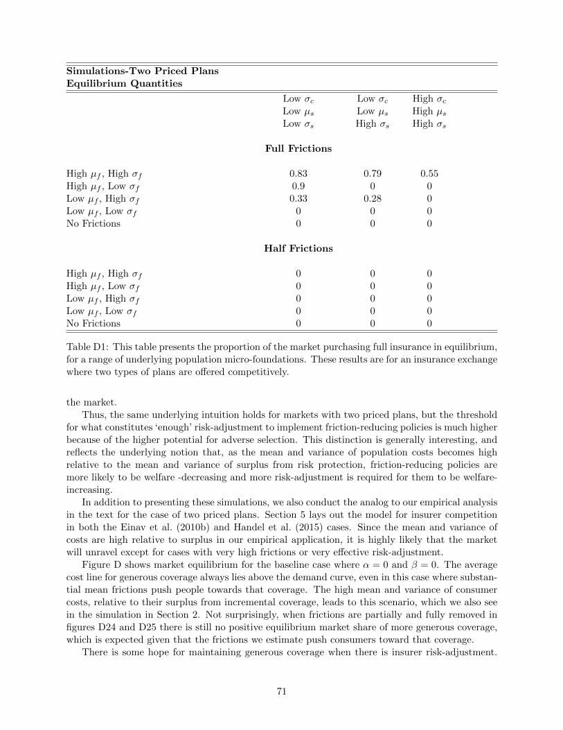
Simulations-Two Priced PlansEquilibrium Quantities

Low σc Low σc High σcLow µs Low µs High µsLow σs High σs High σs

Full Frictions

High µf , High σf 0.83 0.79 0.55High µf , Low σf 0.9 0 0Low µf , High σf 0.33 0.28 0Low µf , Low σf 0 0 0No Frictions 0 0 0

Half Frictions

High µf , High σf 0 0 0High µf , Low σf 0 0 0Low µf , High σf 0 0 0Low µf , Low σf 0 0 0No Frictions 0 0 0

Table D1: This table presents the proportion of the market purchasing full insurance in equilibrium,for a range of underlying population micro-foundations. These results are for an insurance exchangewhere two types of plans are offered competitively.

the market.Thus, the same underlying intuition holds for markets with two priced plans, but the threshold

for what constitutes ‘enough’ risk-adjustment to implement friction-reducing policies is much higherbecause of the higher potential for adverse selection. This distinction is generally interesting, andreflects the underlying notion that, as the mean and variance of population costs becomes highrelative to the mean and variance of surplus from risk protection, friction-reducing policies aremore likely to be welfare -decreasing and more risk-adjustment is required for them to be welfare-increasing.

In addition to presenting these simulations, we also conduct the analog to our empirical analysisin the text for the case of two priced plans. Section 5 lays out the model for insurer competitionin both the Einav et al. (2010b) and Handel et al. (2015) cases. Since the mean and variance ofcosts are high relative to surplus in our empirical application, it is highly likely that the marketwill unravel except for cases with very high frictions or very effective risk-adjustment.

Figure D shows market equilibrium for the baseline case where α = 0 and β = 0. The averagecost line for generous coverage always lies above the demand curve, even in this case where substan-tial mean frictions push people towards that coverage. The high mean and variance of consumercosts, relative to their surplus from incremental coverage, leads to this scenario, which we also seein the simulation in Section 2. Not surprisingly, when frictions are partially and fully removed infigures D24 and D25 there is still no positive equilibrium market share of more generous coverage,which is expected given that the frictions we estimate push consumers toward that coverage.

There is some hope for maintaining generous coverage when there is insurer risk-adjustment.

71

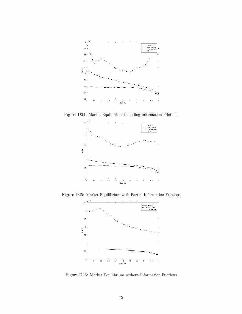
Figure D24: Market Equilibrium Including Information Frictions

Figure D25: Market Equilibrium with Partial Information Frictions

Figure D26: Market Equilibrium without Information Frictions

72

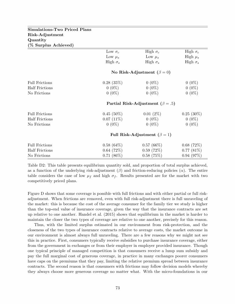
Simulations-Two Priced PlansRisk-AdjustmentQuantity(% Surplus Achieved)

Low σc High σc High σcLow µs Low µs High µsHigh σs High σs High σs

No Risk-Adjustment (β = 0)

Full Frictions 0.28 (35%) 0 (0%) 0 (0%)Half Frictions 0 (0%) 0 (0%) 0 (0%)No Frictions 0 (0%) 0 (0%) 0 (0%)

Partial Risk-Adjustment (β = .5)

Full Frictions 0.45 (50%) 0.01 (2%) 0.25 (30%)Half Frictions 0.07 (11%) 0 (0%) 0 (0%)No Frictions 0 (0%) 0 (0%) 0 (0%)

Full Risk-Adjustment (β = 1)


Table D2: This table presents equilibrium quantity sold, and proportion of total surplus achieved,as a function of the underlying risk-adjustment (β) and friction-reducing policies (α). The entiretable considers the case of low µf and high σf . Results presented are for the market with twocompetitively priced plans.

Figure D shows that some coverage is possible with full frictions and with either partial or full risk-adjustment. When frictions are removed, even with full risk-adjustment there is full unraveling ofthe market: this is because the cost of the average consumer for the family tier we study is higherthan the top-end value of insurance coverage, given the way that the insurance contracts are setup relative to one another. Handel et al. (2015) shows that equilibrium in the market is harder tomaintain the closer the two types of coverage are relative to one another, precisely for this reason.

Thus, with the limited surplus estimated in our environment from risk-protection, and thecloseness of the two types of insurance contracts relative to average costs, the market outcome inour environment is almost always full unraveling. There are a few reasons why we might not seethis in practice. First, consumers typically receive subsidies to purchase insurance coverage, eitherfrom the government in exchanges or from their employer in employer provided insurance. Thoughone typical principle of managed competition is that consumers receive a lump sum subsidy andpay the full marginal cost of generous coverage, in practice in many exchanges poorer consumershave caps on the premiums that they pay, limiting the relative premium spread between insurancecontracts. The second reason is that consumers with frictions may follow decision models wherebythey always choose more generous coverage no matter what. With the micro-foundations in our

73

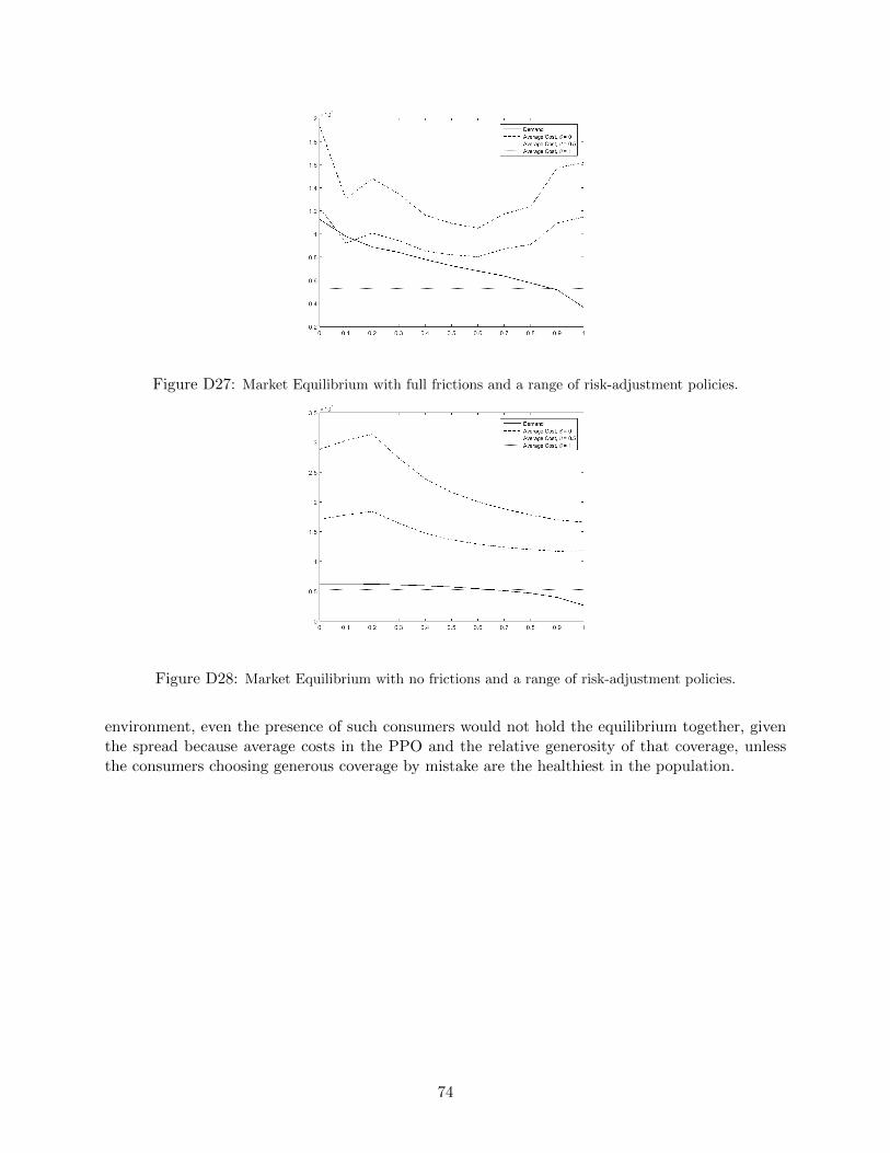
Figure D27: Market Equilibrium with full frictions and a range of risk-adjustment policies.

Figure D28: Market Equilibrium with no frictions and a range of risk-adjustment policies.

environment, even the presence of such consumers would not hold the equilibrium together, giventhe spread because average costs in the PPO and the relative generosity of that coverage, unlessthe consumers choosing generous coverage by mistake are the healthiest in the population.

74

E Appendix: Additional Analysis

Table E presents summary demographic statistics for the samples we study. The first columnrepresents all employees who were present in our data and have complete records for at least eightmonths in the four years of data (t1-t4) that we observe.65 The second column represents allemployees who received our survey, regardless of whether or not they responded. The third columnrepresents all employees who responded to our survey. Statistics from gender onwards representonly t3, and use the re-weighted statistics for the second and third columns, as described in thetext.

Table E2 presents the details of plan design for the two plans consumers choose between in ourempirical environment. Table E4 presents the results for the simulations in Section 2.5 that are forthe case of partially effective friction-reducing policies (α = 0.5). Table E3 describes the proportionof consumers making choice mistakes in each of the simulation scenarios described in Section 2.5.

65We cannot provide the exact number of overall employees, to preserve the anonymity of the firm. As noted earlier,we cannot state the exact years of the data, though we note they are from a four-year period between 2008-2014.

75

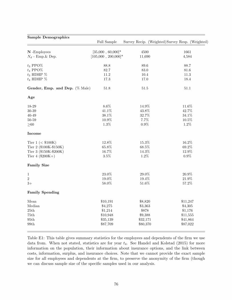
Sample DemographicsFull Sample Survey Recip. (Weighted)Survey Resp. (Weighted)

N -Employees [35,000 , 60,000]* 4500 1661Nd - Emp.& Dep. [105,000 , 200,000]* 11,690 4,584

t3 PPO% 88.8 89.6 88.7t4 PPO% 82.7 83.0 81.6t3 HDHP % 11.2 10.4 11.3t4 HDHP % 17.3 17.0 18.4

Gender, Emp. and Dep. (% Male) 51.8 51.5 51.1

Age

18-29 8.6% 14.9% 11.6%30-39 41.1% 43.8% 42.7%40-49 38.1% 32.7% 34.1%50-59 10.9% 7.7% 10.5%≥60 1.3% 0.9% 1.2%

Income

Tier 1 (< $100K) 12.8% 15.3% 16.2%Tier 2 ($100K-$150K) 65.8% 68.5% 69.2%Tier 3 ($150K-$200K) 16.7% 14.3% 12.9%Tier 4 ($200K+) 3.5% 1.2% 0.9%

Family Size

1 23.0% 29.0% 20.9%2 19.0% 19.4% 21.9%3+ 58.0% 51.6% 57.2%

Family Spending

Mean $10,191 $8,820 $11,247Median $4,275 $3,363 $4,30525th $1,214 $878 $1,17675th $10,948 $9,388 $11,55595th $35,139 $32,171 $41,86499th $87,709 $80,370 $87,022

Table E1: This table gives summary statistics for the employees and dependents of the firm we usedata from. When not stated, statistics are for year t4. See Handel and Kolstad (2015) for moreinformation on the population, their information about insurance options, and the link betweencosts, information, surplus, and insurance choices. Note that we cannot provide the exact samplesize for all employees and dependents at the firm, to preserve the anonymity of the firm (thoughwe can discuss sample size of the specific samples used in our analysis.

76

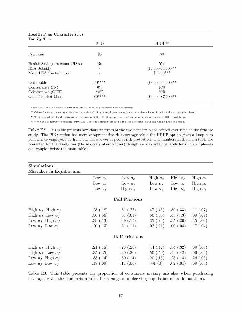
Health Plan CharacteristicsFamily Tier

PPO HDHP*

Premium $0 $0

Health Savings Account (HSA) No YesHSA Subsidy - [$3,000-$4,000]**Max. HSA Contribution - $6,250***

Deductible $0**** [$3,000-$4,000]**Coinsurance (IN) 0% 10%Coinsurance (OUT) 20% 30%Out-of-Pocket Max. $0**** [$6,000-$7,000]**

* We don’t provide exact HDHP characteristics to help preserve firm anonymity.

**Values for family coverage tier (2+ dependents). Single employees (or w/ one dependent) have .4× (.8×) the values given here.

***Single employee legal maximum contribution is $3,100. Employees over 55 can contribute an extra $1,000 in ’catch-up.’

****For out-of-network spending, PPO has a very low deductible and out-of-pocket max. both less than $400 per person.

Table E2: This table presents key characteristics of the two primary plans offered over time at the firm westudy. The PPO option has more comprehensive risk coverage while the HDHP option gives a lump sumpayment to employees up front but has a lower degree of risk protection. The numbers in the main table arepresented for the family tier (the majority of employees) though we also note the levels for single employeesand couples below the main table.

SimulationsMistakes in Equilibrium


Full Frictions

High µf , High σf .23 (.18) .31 (.27) .47 (.45) .36 (.33) .11 (.07)High µf , Low σf .56 (.56) .61 (.61) .50 (.50) .43 (.43) .09 (.09)Low µf , High σf .39 (.13) .39 (.15) .35 (.24) .35 (.20) .35 (.06)Low µf , Low σf .26 (.13) .21 (.11) .02 (.01) .06 (.04) .17 (.04)

Half Frictions

High µf , High σf .21 (.18) .28 (.26) .44 (.42) .34 (.32) .09 (.06)High µf , Low σf .35 (.35) .30 (.30) .50 (.50) .42 (.42) .09 (.09)Low µf , High σf .33 (.14) .30 (.14) .20 (.15) .23 (.14) .26 (.06)Low µf , Low σf .17 (.09) .11 (.06) .01 (0) .02 (.01) .09 (.03)

Table E3: This table presents the proportion of consumers making mistakes when purchasingcoverage, given the equilibrium price, for a range of underlying population micro-foundations.

77

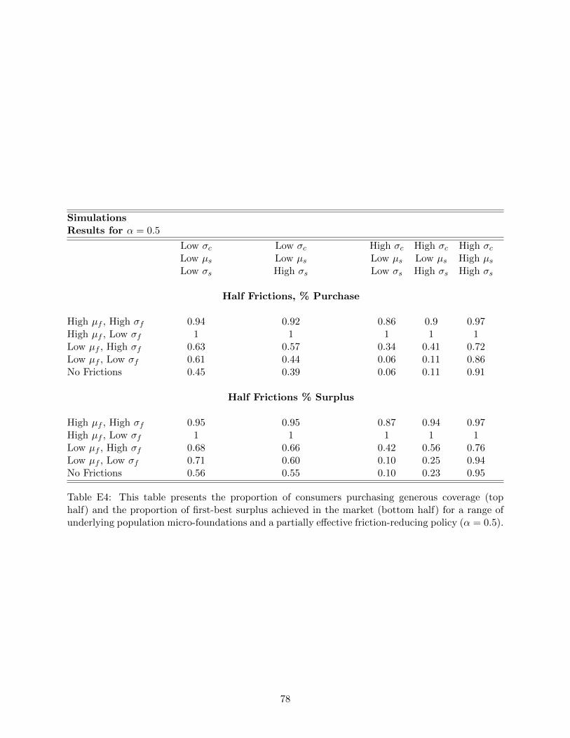
SimulationsResults for α = 0.5


Half Frictions, % Purchase


Half Frictions % Surplus


Table E4: This table presents the proportion of consumers purchasing generous coverage (tophalf) and the proportion of first-best surplus achieved in the market (bottom half) for a range ofunderlying population micro-foundations and a partially effective friction-reducing policy (α = 0.5).

78

Documents

Information Frictions and Adverse Selection: Policy