NBER WORKING PAPER SERIES

INFORMATION DIFFUSION EFFECTS IN INDIVIDUAL INVESTORS' COMMON STOCK PURCHASES:COVET THY NEIGHBORS' INVESTMENT CHOICES

Zoran IvkovichScott Weisbenner

Working Paper 13201http://www.nber.org/papers/w13201

NATIONAL BUREAU OF ECONOMIC RESEARCH1050 Massachusetts Avenue

Cambridge, MA 02138June 2007

We extend our gratitude to an anonymous discount broker for providing the data on individual investors'positions, trades, and demographics. Special thanks go to Terry Odean for his help in obtaining andunderstanding the data set. Both authors acknowledge the financial support from the College ResearchBoard at the University of Illinois at Urbana-Champaign. We thank Jean Roth of the NBER for assistancewith the 1990 Census data. We also thank seminar participants at the University of Florida and theUniversity of Illinois for their comments and feedback. The views expressed herein are those of theauthors and not necessarily those of the National Bureau of Economic Research. The views expressedherein are those of the author(s) and do not necessarily reflect the views of the National Bureau ofEconomic Research.

© 2007 by Zoran Ivkovich and Scott Weisbenner. All rights reserved. Short sections of text, not toexceed two paragraphs, may be quoted without explicit permission provided that full credit, including© notice, is given to the source.

Information Diffusion Effects in Individual Investors' Common Stock Purchases: Covet ThyNeighbors' Investment ChoicesZoran Ivkovich and Scott WeisbennerNBER Working Paper No. 13201June 2007JEL No. D14,D83,G11

ABSTRACT

We study the relation between households' stock purchases and stock purchases made by their neighbors.A ten percentage point increase in neighbors' purchases of stocks from an industry is associated witha two percentage point increase in households' own purchases of stocks from that industry. The effectis considerably larger for local stocks and among households in more social states. Controlling forarea sociability, households' and neighbors' investment style preferences, and the industry compositionof local firms, we attribute approximately one-quarter to one-half of the correlation between households'stock purchases and stock purchases made by their neighbors to word-of-mouth communication.

Zoran IvkovichDepartment of FinanceUniversity of Illinois340 Wohlers Hall1206 South Sixth StreetChampaign, IL 61820ivkovich@uiuc.edu

Scott WeisbennerDepartment of FinanceUniversity of Illinois, Urbana-Champaign304C David Kinley Hall1407 W. Gregory DriveUrbana, IL 61801and NBERweisbenn@uiuc.edu

Despite the fact that individuals collectively hold about one-half of the U.S. stock market,

information diffusion effects among individual investors—the relation between the investment

choices made by an individual investor’s neighborhood and the investor’s own investment

choices—have received relatively little attention in the academic literature, probably because of

the lack of detailed data. If present, such effects undoubtedly can affect individual investors’

asset allocation decisions. Moreover, trades based on information diffusion might be sufficiently

correlated and condensed in time to affect stock prices.

In the domain of institutional investors, Hong, Kubik, and Stein (2005) study word-of-

mouth effects among mutual fund managers and find that “…a manager is more likely to hold (or

buy, or sell) a particular stock in any quarter if other managers in the same city are holding (or

buying, or selling) that same stock.” This study complements their work by ascertaining whether

such trading patterns are a broader phenomenon. For example, individual investors may seek to

reduce search costs and circumvent their lack of expertise by relying on word-of-mouth

communication with those around them. Indeed, Hong, Kubik, and Stein (2004) present a model

in which stock market participation may be influenced by social interaction. Such social

interaction can serve as a mechanism for information exchange via “word-of-mouth” and/or

“observational learning” (Banerjee (1992), Ellison and Fudenberg (1993, 1995)). Duflo and Saez

(2002, 2003) present evidence of peer effects in the context of retirement plans. They find that an

employee’s participation in retirement plans and choices within those plans are affected by

participation decisions and choices made by other employees in the same department.

In the international arena, Feng and Seasholes (2004) present evidence of herding effects

among individual investors who hold individual brokerage accounts in the People’s Republic of

China. A unique feature of their data (investors seeking to place trades in person can` do so only

1

in the brokerage house in which they opened their accounts) enables Feng and Seasholes to

disentangle word-of-mouth effects from common reaction to releases of public information.

They find that common reaction to public information (trades placed across branches in the same

region, local to the company), rather than word-of-mouth effects (trades placed in the same

branch), seems to be a primary determinant of herding in that context.

Grinblatt and Keloharju (2001) find that proximity to corporate headquarters, the

language of communication with investors, and the company’s CEO’s cultural origin are

important determinants of Finnish households’ stock investments. Whereas these findings could

be consistent with word-of-mouth effects influencing portfolio choice, they could also reflect

households’ tastes for familiarity—preference to invest in companies that disseminate annual

financial reports in their native tongues or feature a CEO with the same origin.

We study information diffusion effects among U.S. individual investors by using a

detailed data set of common-stock investments 35,673 U.S. households made through a large

discount brokerage in the period from 1991 to 1996. Throughout the paper, we loosely refer to

the correlation between households’ investments and their neighbors’ investments as

“information diffusion.” This term is intended to encapsulate several potential reasons why such

correlation exists—word-of-mouth effects, similarity in preferences, as well as common local

reaction to news. To further characterize information diffusion and word-of-mouth effects, we

consider state-level measures of sociability and find that the level of sociability prevailing in the

state to which the household belongs (likely a strong correlate of the presence of word-of-mouth

effects) can explain a significant portion of the overall diffusion effect. Moreover, we

disentangle the diffusion into the influences of common preferences, structure of the local

industry, and word-of-mouth effects.

2

Putting our results in perspective and comparing them with the findings from Feng and

Seasholes (2004) delivers a new, richer understanding of the different mechanisms that govern

individuals’ investment decisions across various societies. Indeed, whereas Feng and Seasholes

(2004) report that individual investors’ correlated investment decisions are driven by common

reaction to locally-available news, with no evidence of word-of-mouth effects among Chinese

investors, our estimates suggest that word-of-mouth effects among U.S. investors are strong,

particularly in more social areas. This discrepancy is consistent with the differences in the

fundamental characteristics of the two societies. Freedom House, which has been producing

annual ratings of political and civil rights for more than 200 countries for the past three decades

(Freedom House (2004)), has ranked the U.S. among the highest and the People’s Republic of

China among the lowest along the dimension of civil liberties. An essential ingredient of the civil

liberties score is prevalence of open and free discussion (or absence thereof). Coupled with the

fact that many, if not most companies in the People’s Republic of China are at least partly

government-owned, it is very plausible that exchanging investment-relevant information in a

society deprived of open and free discussion and many other civil liberties is rare and modest.

Even within the U.S., there is variation in sociability (e.g., membership in clubs, trust in

other people). If word-of-mouth is an important contributor to households’ stock purchases, the

observed correlation in a household’s portfolio allocation and that of its neighbors should be

higher in the more social areas. Other explanations for information diffusion effects, such as

correlated preferences and common local reaction to news, should not vary with the sociability

of the community. Using state-level variation in sociability measures enables us to differentiate

among the competing hypotheses that can explain trading patterns of U.S. investors.

3

Overall, we find a strong information diffusion effect (“neighborhood effect”): a ten

percentage point increase in purchases of stocks from an industry made by a household’s

neighbors is associated with an increase of two percentage points in the household’s own

purchases of stocks from that industry. We pay particular attention to the differentiation between

information diffusion effects related to local stocks (defined as companies headquartered within

50 miles from the household) and the effects related to non-local stocks. Whereas the key

neighborhood effects—similarity in preferences, the impact of the structure of the local industry,

and word-of-mouth—can prevail among the investments both local and non-local to the

household, most of those effects will likely be far more pronounced among local investments

because, as demonstrated for both professional money managers (Coval and Moskowitz (2001))

and individual investors (Ivković and Weisbenner (2005)), the flow of value-relevant

information regarding local companies appears to be higher and of better quality than the

comparable flow regarding remote, non-local companies.

Not surprisingly, we indeed find that information diffusion effects are considerably

stronger for local purchases than for non-local ones. For example, if the neighborhood’s

allocation of local purchases to a particular industry increases by ten percentage points, a

household tends to increase its own allocation of local purchases to the industry by a comparable

amount. This result adds another dimension to the already documented high degrees of

individual investors’ locality, both in the U.S. (Ivković and Weisbenner (2005), Zhu (2002)) and

abroad (Grinblatt and Keloharju (2001), Massa and Simonov (2006)): not only do investors tend

disproportionately to invest locally, but there are also strong information diffusion effects in their

neighborhood.

4

We further find that a household’s sensitivity to neighbors’ investment choices increases

with the population of the household’s community. Such diffusion in stock trading affects

individual investors’ asset allocation decisions. For example, although residents in larger

metropolitan areas have substantially more diverse investment opportunities and tend to invest

more in local stocks, we find that their local stock investments tend to remain just as

concentrated as those made by residents of less populated communities (who have a significantly

smaller pool of potential local investments). This tendency is consistent with the notion that

residents in more populous geographic areas might be exposed to word-of-mouth effects to a

higher degree than residents in less highly populated areas.

Finally, to disentangle the contributions of correlated preferences and the structure of the

local economy to the observed correlation between individual investors’ stock purchases and

those of their neighbors from “word-of-mouth” effects, we conduct two tests. First, we consider

the level of sociability of the state to which the household belongs and find that the relation

between industry-level household purchases and neighborhood purchases is substantially

stronger among households in the more sociable states. Second, we consider the households’

own preferences (as revealed by the composition of their respective portfolios across industries

at the beginning of each quarter), preferences of the households’ respective neighborhoods (as

revealed by the composition of the neighborhoods’ aggregate portfolios), as well as the

composition of local firms and workers by industry. We find that one-quarter to one-half of the

overall diffusion effect among both local and non-local investments cannot be attributed to these

sources. We regard the remaining portions of the diffusion effect as a conservative lower bound

on the impact of word-of-mouth communication effects on household trading decisions.

Disentangling the overall information diffusion effect into word-of mouth communication and

5

other diffusion effects potentially yields further insight as to how correlated trading among

individuals may influence stock prices.

Our results complement and extend those of Hong, Kubik, and Stein (2005), suggesting

that word-of-mouth effects are a broad phenomenon that affects financial decisions made by both

mutual fund managers and individual investors. The two studies provide evidence supportive of

word-of-mouth effects using different techniques, thereby adding to the robustness of the overall

finding. Hong, Kubik, and Stein (2005) rule out alternative explanations for correlated trading

patterns by examining trading activity before and after Regulation FD and by focusing on trades

in stocks for which investor relations are unlikely to be a contributing factor (stocks not local to

the managers and small stocks). In this paper, we disentangle possible explanations for correlated

trading patterns by exploiting differences in sociability of communities across the U.S., as well

as introducing several controls for similarity in investment preferences within the community (as

manifested by previous household investment decisions) and the composition of the local

economy.

The remainder of this paper is organized as follows. Section 1 describes the data and

summary statistics. We present our basic findings concerning information diffusion, the impact

of the size of the population residing in the household’s community, and dissipation of diffusion

effects with distance from the household in Section 2. We examine the role of sociability and

identify the contributions of correlated preferences, the structure of the local economy, and

word-of-mouth communication to overall diffusion in individuals’ investment choices in Section

3. Section 4 concludes.

6

1. Data and Descriptive Statistics

1.1 Data

The primary data set, obtained from a large discount broker, consists of individual investors’

monthly positions and trades over a six-year period from 1991 to 1996. It covers the investments

that 78,000 households made through the discount broker, including common stocks, mutual

funds, and other securities. Each household could have as few as one and as many as 21 accounts

(the median number of accounts per household is two). The information associated with each

trade includes the account in which the trade was made. A separate data file contains the

information associated with each account, including the household to which the account belongs.

This structure of the data allows us to associate with each trade the household that made it. For

further details see Barber and Odean (2000).

In this paper we focus on the common stocks traded on the NYSE, AMEX, and Nasdaq

exchanges. Common stock investments constitute roughly three-quarters of the total value of

household investments through the brokerage house in the sample. We use the Center for

Research in Security Prices (CRSP) database to obtain information on stock prices and returns

and COMPUSTAT to obtain several firm characteristics, including company headquarters

location (identified by its state and county codes). We use the headquarters location as opposed

to the state of incorporation because firms often do not have the majority of their operations in

their state of incorporation.1

We exclude the stocks that we could not match with CRSP and COMPUSTAT; they were

most likely listed on smaller exchanges. We also exclude stocks not headquartered in the

continental U.S. The resulting “market”—the universe of stocks about which we could obtain

the necessary characteristics and information—is representative of the overall market. For

7

example, at the end of 1991 the “market” consists of 5,478 stocks that cover 89% of the overall

market capitalization at the time.

The sample of households used in this study is a subset of the entire collection of

households for which we could ascertain their zip code and thus determine their location. We

obtained the latitude and longitude for each of the zip codes from the U.S. Census Bureau’s

Gazetteer Place and Zip Code Database. Company locations come from the COMPUSTAT

Annual Research Files, which contain the information regarding company headquarters’ county

codes. Finally, we identify the latitude and longitude for each county from the U.S. Census

Bureau’s Gazetteer Place and Zip Code Database as well. We use the standard formula for

computing the distance d(a,b) in statutory miles between two points a and b as follows:

d(a,b) = arccos{cos(a1)cos(a2)cos(b1)cos(b2)+cos(a1)sin(a2)cos(b1)sin(b2)+sin(a1)sin(b1)} r, (1)

where a1 and b1 (a2 and b2) are the latitudes (longitudes) of the two points (expressed in radians),

respectively, and r denotes the radius of the Earth (approximately 3,963 statutory miles).

The sample size necessitates two adjustments. First, instead of fitting regressions based

on individual stocks we aggregate all the buys in each quarter by assigning firms to one of the

following 14 industry groups based on their SIC codes: mining, oil and gas, construction, food,

basic materials, medical/biotechnology, manufacturing, transportation, telecommunications,

utilities, retail/wholesale trade, finance, technology, and services. Moreover, although 35,673

households purchased common stocks at some point during the sample period, in each quarter

we consider only the households that made some purchases during the quarter. In sum, there are

23 complete quarters in the sample period (1991:1 to 1996:3), 14 industries, and 7,000 to 9,000

households that made stock purchases in a quarter. This leads to a total of 2,678,004

8

observations, where each observation has several control variables, as well as 322 industry-

quarter dummy variables (14 industries x 23 quarters).

In most analyses, we relate the industry composition of a household’s purchases during a

quarter to the industry composition of all the purchases of the household’s neighbors (households

located within 50 miles) made during the quarter, plus appropriate controls. We choose this

distance because there is evidence that 50 miles captures most of one’s social interactions.2

Finally, in some analyses we relate the extent of information diffusion to the sociability

that prevails in the area surrounding the household. To capture sociability, we use state-level

values of the Comprehensive Social Capital Index, as collected and presented in Putnam (2000).3

We classify households according to their state’s Comprehensive Social Capital Index and split

the sample of households into sociable and non-sociable ones, where the breakpoint is the

sociability measure of the median household in the sample.4

1.2 Summary Statistics

Table 1 summarizes quarterly household stock purchases at the industry level. Summary

statistics are reported annually, as well as for the entire sample period (bottom row of the table).

The first column presents the number of household-quarter-industry (h, t, i) combinations in a

given year such that household h made at least one purchase in quarter t in industry i. The second

column tallies the number of distinct households appearing in the sample in a given year. The

third column lists average dollar values of households’ quarterly purchases, where median values

are reported in parentheses underneath the mean values. The last column breaks down the

purchases according to their distances from the household (i.e., whether the firm headquarters is

located within 50 miles of the household). There are a total of 191,286 “purchases”—household-

quarter-industry (h, t, i) combinations for which there was a purchase by household h in quarter t

9

in industry i—with 16,000-20,000 households making purchases each year, for a total of 35,673

distinct households throughout the sample period. The distribution of the dollar values of

quarterly purchases is skewed; whereas the mean quarterly purchase was around $29,000, the

median value was substantially smaller, around $8,000. The fourth column shows individual

investors’ disproportionate preference for local stocks (17.1% of all purchases), a phenomenon

studied in Ivković and Weisbenner (2005) and Zhu (2002).

2. Information Diffusion Effects

2.1 Basic Regression Specification

We begin by classifying individual stock purchases made by household h in quarter t into

industries i = 1, 2, … , 14 and compute fh,t,i, the dollar-weighted share of a household’s quarterly

buys in each industry.5 In various analyses, the aggregation into 14 industries is done across all

stock purchases, local purchases only, and non-local purchases only. Moreover, for each

household h and each quarter t we also compute , i = 1, 2, … , 14, that is, the proportion

of buys made by all neighboring households within 50 miles from household h (excluding

household h) in each of the 14 industries. For presentational convenience, throughout the paper

the household industry shares f

50,, ithF−

h,t,i are expressed in percentage points (that is, they are multiplied

by 100), whereas neighboring household industry shares are not. Finally, we employ industry-

quarter effects to allow for market-wide variation in demand across industries and time by

defining 322 dummy variables Dt,i, t = 1, …, 23 (from quarter 1991:1 to 1996:3), and i = 1, 2, …

, 14. These controls ensure that our results are not driven by, for example, technology stocks

beating analysts’ expectations, which belong to the common information set that may affect

10

buying patterns of all investors, but rather reflect the differences in households’ propensity to

purchase technology stocks across different communities. In sum, the basic regression is:

(2) itht i

ititithith DFf ,,23

1

14

1,,

50,,,, εγβ ∑ ∑

= =− ++=

For the basic specification without controls other than the 322 dummy variables, the null

hypothesis is that information diffusion effects (“neighborhood effects”) do not exist, that is, that

the coefficient β is zero. A positive β would suggest the presence of information diffusion

effects.

We next address the correlation structure of the error term: observations are independent

neither within each household-quarter combination (industry shares necessarily need to add up to

one) nor across time (households’ preferences are unlikely to change at quarterly frequency). It

follows that the OLS regression estimation, although consistent, would produce biased standard

errors. Thus, we report the standard errors and resulting tests of statistical significance based

upon a robust estimator that clusters observations at the household-quarter level for all

regressions.

There are several reasons why U.S. individuals’ investment choices might be related to

those made by their neighbors. At the outset, we note that individual investors might be reacting

to the same publicly available information to which their neighbors are reacting. Such tendencies

may cause correlated trading. Indeed, Barber, Odean, and Zhu (2006) document that trading

patterns are correlated across individual investors and Barber and Odean (2005) find that

individual investors are inclined to buy stocks that have attracted attention. These correlated

trading patterns are not necessarily surprising in light of exposure to (the same) publicly

11

available information, as well as to the pronounced presence of the disposition effect (Odean,

1998), tax-motivated trading (Ivković, Poterba, and Weisbenner (2005)), or other behavioral

phenomena that might prevail among individual investors, yet need not be driven by information

diffusion effects. Our basic set of 322 industry-quarter dummy variables seeks to control for

these and other trading factors that do not vary across communities (e.g., when a stock price

reaches an all-time high, it does so for all investors) and thereby to allow our specifications to

pick up information diffusion effects.

2.2 Information Diffusion Effects for Purchases

We present the results of fitting the regression from Equation (2) in Panel A of Table 2. Within

the panel, each row pertains to a different dependent variable. The first row of the panel pertains

to the industry share breakdown fh,t,i computed across all buys. Running the basic regression,

without any controls other than the 322 industry-quarter dummies, produces the highly

statistically significant estimate of 20.7 and thus suggests that a 10 percentage point change in

the neighbors’ allocation of purchases in an industry is associated with a nearly 2.1 percentage

point change in the household’s own allocation of purchases in the industry.6

As discussed in the introduction, information diffusion that prevails among local and

non-local stocks may be different. Similarity in preferences, the structure of the local industry,

and word-of-mouth effects are likely stronger among local investments. This inquiry is also

motivated by studies of local bias among both institutional investors (Coval and Moskowitz

(1999)) and individual investors (Ivković and Weisbenner (2005) and Zhu (2002)). These studies

find that both groups of investors are biased toward holding disproportionately more local stocks

in their portfolios. Moreover, Coval and Moskowitz (2001) and Ivković and Weisbenner (2005)

12

present evidence that local investments outperformed non-local ones among mutual fund

managers and individual investors, respectively.

Separate consideration of local purchases7 and non-local purchases, reported in the next

two rows of Table 2, Panel A, indeed reveals that local information diffusion effects are larger

than the non-local ones by an order of magnitude (119.3 vs. 8.4). For example, if the

neighborhood’s allocation of purchases to a particular industry increases by ten percentage

points, a household tends to increase its own allocation of local purchases to the industry by a

comparable amount. This result adds another dimension to the already documented high degrees

of individual investors’ locality, both in the U.S. (Ivković and Weisbenner (2005), Zhu (2002))

and overseas (Grinblatt and Keloharju (2001), Massa and Simonov (2006)), by suggesting the

possibility that strong information diffusion effects could contribute to individual investors’ local

bias.

2.3 Information Diffusion Effects for Sales and Positions

In Panels B and C of Table 2 we also examine the extent to which households’ sale and holding

decisions are correlated with those of their neighbors. We find a similar pattern of results for sale

decisions as we do for purchase decisions. For example, estimates from Panel B suggest that a 10

percentage point change in the neighbors’ sales of stock in an industry is associated with a 3.0

percentage point change in the household’s own sales of stock in the industry.

Perhaps not surprisingly, the correlation between the composition of a household’s

positions across industries and that of their neighbors is substantially larger than those for

purchases (the coefficients are larger in magnitude by 50% to 100% across the three samples).

This larger correlation reflects the fact that positions are the combination of both past purchase

decisions and the returns accrued on those investments. The larger correlation for positions

13

relative to trades mirrors the results reported for mutual fund managers in Hong, Kubik, and

Stein (2005).

For the remainder of the paper, we focus on households’ purchase decisions because they

are unconstrained, that is, households are free to purchase any stock, and they represent

households’ active financial decisions. By contrast, in the absence of short selling, sale decisions

are limited to the stocks already held (essentially no investors in our sample sold stocks short).

Thus, a correlation in selling activity could simply represent an underlying correlation in the

original buying activity of those stocks. Moreover, a correlation in positions could in part simply

reflect households’ inertia, as households could hold similar stocks over a long period of time

(and thus experience similar movements in the value of their portfolio positions).8

2.4 Information Diffusion Effects and Local Population Size

In this section we stratify households according to the size of the population that resides within

50 miles from the household. We define four categories: 0-1 million residents, 1-2.5 million

residents, 2.5-5 million residents, and more than 5 million residents. Not surprisingly, the size of

the local population and the diversity of local companies are positively related (i.e., local

population and the Herfindahl index of industry concentration are negatively correlated).

Specifically, the Herfindahl index of the industry composition of firms local to the average

household decreases from around 0.5 to around 0.2 as the population increases from 0-1 million

local residents to more than 5 million local residents.9 Yet, although the average dollar amount

of quarterly purchases of local individual stocks increases from $13,000 to $22,400 as the size of

the local population increases from 0-1 million to more than 5 million local residents, the

Herfindahl index of households’ local purchases across industries remains virtually unchanged—

it drops only very slightly from 0.99 to 0.95. Thus, although residents in larger metropolitan

14

areas have substantially more diverse investment opportunities and tend to invest more into local

stocks, they tend to remain very focused in their industry allocation. This tendency is consistent

with the notion that residents in more populous geographic areas might be exposed to

information diffusion effects to a higher degree than residents in less highly populated areas. To

confirm this intuition, we run a simple modification of the basic regression from Equation (2) on

subsamples selected by the type of purchase (all buys, local buys, and non-local buys) wherein

information diffusion effects are interacted with indicator variables representing local population

size (0-1 million, 1-2.5 million, 2.5-5 million, more than 5 million). The coefficient estimate

presented in the table for a particular population group represents the total information diffusion

effect for that group (i.e., the sum of the diffusion effect for the 0-1 million group and the

interaction term for that particular population group).

Across all three regressions presented in Table 3, information diffusion effects in

purchases increase with population size. Stronger effects in larger metropolitan areas may stem

from a greater flow of investment-relevant information through increased availability of

information sources (e.g., business-oriented magazines and newspapers) and advertising efforts,

both of which are subject to economies of scale and are typically more substantial in larger

metropolitan areas.

2.5 Dissipation of Information Diffusion Effects with Distance from the Household

One would expect information diffusion effects to dissipate as the distance from the household

increases. To test this hypothesis, we define regions surrounding the household at increasingly

larger distances as follows: 0-50 miles, 50-70.7 miles, 70.7-86.6 miles, 86.6-100 miles, … ,

141.4-150 miles. These regions each cover a geographic area of the same size (502 π = 7,854

square miles). We then run a regression similar to Equation (2), except, instead of having one

15

information diffusion regressor , the specification now has nine ( , ,

, , , , , , and ). The results are

presented graphically in Figure 1. Across all three panels, that is, for all buys, local buys, and

non-local buys, the pattern is the same: there is a rapid and fairly steady exponential decline of

the information diffusion coefficients with distance from the household. As one might suspect, a

household’s purchases of non-local stocks are relatively more sensitive to the decisions made by

members of more distant communities than its purchases of local stocks are. That is, going

beyond the 50-mile community leads to a substantially faster decline in information diffusion

effects in the domain of local stocks than in the domain of non-local stocks.

50,, ithF−

50,, ithF−

7150,,−ithF

8771,,−ithF 10087

,,−ithF 112100

,,−

ithF 122112,,−

ithF 132122,,−

ithF 141132,,−

ithF 150141,,−ithF

2.6 Robustness Checks

An issue of potential concern for local information diffusion is that the effect might be driven by

some form of inside trading: those who work for a company may be trading in their own

company stock and may be selectively releasing pertinent information to their relatives and close

friends. We regard this effect as somewhat distinct from the other aspects of information

diffusion because the information the investors would receive is likely much more precise than

the information available through word-of-mouth effects, exposure to local news, influence of

company’s presence through advertising efforts, company-sponsored events, or social interaction

with company employees.

Unfortunately, the data set does not provide information about the investors’ current and

past employers. We control for the own-company stock explanation, however, by focusing on the

plausible assumption that, if a household’s local purchase is motivated by inside information, it

is likely to be the household’s largest local trade in that quarter. Accordingly, we compute for

16

each household h in quarter t the industry composition of local purchases excluding the single

largest stock purchase made by household h in quarter t. In unreported analyses, we find that this

specification yields estimates of the local information diffusion effect that are even somewhat

larger than the estimates based on the full sample of local investments (152.5 versus 119.3).

Therefore, we do not find evidence that trading in own-company stock drives the estimated

information diffusion effects among local investments.

Another issue of potential concern is that the estimates of local information diffusion may

be induced by the dominant presence of a company (or industry) in a household’s neighborhood.

Taking a drastic example, suppose there is only one company (or multiple companies all

belonging to the same industry) local to the household. The opportunity set for local investments

is therefore very focused and the inability to invest locally into any other industry may bias the

results. To assess the impact of industry dominance in the local opportunity set, in unreported

analyses we estimate regressions for local purchases on a subsample of purchases—household-

quarter-industry (h,t,i) combinations for which the weight of industry i in the portfolio of firms

local to household h does not exceed the threshold of 50%, that is, the observations not plagued

by the domination of a single company (or industry) in the community. The regression

coefficient remains essentially the same; it declines only very slightly, from 119.3 to 111.3,

which suggests that the “one-company town” issue does not drive local information diffusion.

3. Disentangling Information Diffusion Effects

The results presented in Section 2 suggest that the stock purchases made by households are

strongly related to those made by their neighbors, consistent with word-of-mouth effects playing

a strong role in household investment decisions. However, such a correlation in trading activity

17

could also reflect an underlying similarity in preferences or the industry composition of local

firms. In regard to U.S. investors, studies have found correlated trading patterns both for

institutional investors (Hong, Kubik, and Stein (2005)) and individual investors (Barber, Odean,

and Zhu (2006)). Hong, Kubik, and Stein (2005) consider alternative interpretations to their

finding that mutual fund managers engage in word-of-mouth communication and tilt their

portfolios accordingly. They use three sets of tests to assess the possibility that their results are

driven by inside information obtained by the money managers directly from company executives

(which they tem the “local-investor-relations” activity). First, their results are unaffected even if

all local stocks are excluded from their regressions. Second, their results are robust among

smaller stocks (which, on average, have fewer resources at their disposal to pursue “local-

investor-relations” activities). Finally, Hong, Kubik, and Stein (2005) consider the post-

Regulation FD period and show that their results persist in the aftermath of explicit regulation

that prohibits companies to engage in selective dissemination of information, suggesting once

again that “local-investor-relations” strategies do not drive their regression results.

As Hong, Kubik, and Stein (2005) point out, none of these “local-investor-relations”

alternative explanations are likely to dominate the arena of individual investors. In fact, Feng and

Seasholes (2004) report that Chinese individual investors’ correlated investment decisions are

driven by common reaction to locally-available news, with no evidence of word-of-mouth effects

on stock trades. However, given the differences in the fundamental characteristics of the U.S.

and Chinese societies (i.e., differences in civil liberties such as open and free discussion), it is

plausible that motivations for stock purchases could also be substantially different across the two

cultures.

18

Moreover, it is important to differentiate among competing sources of the overall

information diffusion effect among U.S. individual investors because they likely have different

levels of influence on the market. For example, word-of-mouth effects may create a more

dynamic exchange of information that may lead to a ripple effect of further information

dissemination, which in turn may have an impact on stock prices.

Thus, we devise two alternative strategies to disentangle the sources of the observed

correlation between a household’s stock purchases and those of its neighbors. The first strategy

considers the sociability of a household’s state. Using the comprehensive state-wide sociability

measure from Putnam (2000) (available for all 50 states except Alaska and Hawaii), we assign a

certain level of sociability to every household in our sample, and then define a dummy variable

associated with each household that labels it as a household in either a high or a low sociability

area. We interact that dummy variable with the neighborhoods’ industry-level purchases. Within

the United States, there is variation in sociability (i.e., membership in clubs, trust in other people,

etc.) across states. If word-of-mouth is an important contributor to a household’s stock

purchases, then the observed correlation in a household’s portfolio allocation and that of their

neighbors should be higher in more social areas. Other explanations for information diffusion

effects, such as correlated preferences and common local reaction to news, should not vary with

the sociability of the community. We interpret the coefficients associated with sociability, which

represent the increased influence of neighbors’ investment choices on an individual’s own

portfolio in social areas relative to less social communities, as measures of the word-of-mouth

effects.

The second strategy considers three key contributions to the overall information diffusion

effect, namely, word-of-mouth communication, correlated preferences (which may incorporate

19

common local reaction to news events), and the structure of the local economy. We use the

composition of the neighborhood’s aggregate portfolio to reveal the neighborhood’s preferences

and the accumulation of their reactions to past news. Analogously, we use the composition of a

household’s own portfolio position to reveal its own preferences and accumulated reactions to

past news. We further use the degree of conformity of the household portfolio composition to the

portfolio composition of the neighborhood to identify households with preferences and reactions

similar to their neighbors’, as well as those whose preferences and reactions are very different

from their neighbors’. Upon controlling for the composition of households’ neighborhood

portfolios and households’ own portfolio compositions, as well as the structure of the local

economy, we view the correlation between the household’s stock purchases and those of its

neighbors that survives such rigid controls as a conservative lower bound on the magnitude of

the word-of-mouth effect.

Strikingly, our estimates of the contribution of word-of-mouth communication are very

similar across households that conformed to their neighbors very closely and those that held very

disparate portfolios. This finding is reassuring because it suggests that the strategy we employed

to control for the effect of common preferences and the cumulative common reactions to news

did not lead to materially different estimates of the word-of-mouth effect across the two sets of

households.

3.1 Controlling for Word-of-Mouth Effects: The Area Sociability Proxy

In this section we report the results of the analyses in which we identify a proxy for the word-of-

mouth effect and interact that measure with diffusion coefficients in a regression specification

very similar to that from Equation (2). Our proxy for the word-of-mouth effect is the sociability

of the area surrounding a household. To capture sociability, we use state-level values of the

20

Comprehensive Social Capital Index, as collected and presented in Putnam (2000).10 We define a

dummy variable that indicates high and low area sociability levels by classifying households

according to their state’s Comprehensive Social Capital Index (Putnam, 2000) and splitting the

households into sociable and non-sociable ones (the breakpoint is the sociability measure of the

median household in the sample). Further recognizing that sociability effects may be stronger in

the areas with more population, we also develop a specification in which we interact the

diffusion coefficient with both the sociability dummy and the population measures (as defined in

Section 2.4 and Table 3).

Table 4 presents the results of both analyses across all buys, local buys, and non-local

buys (Panels A, B, and C, respectively). Within each panel, the first section reports regression

results for specifications involving area sociability measures only, whereas the second section

reports results of the more complicated specifications that also include interactions with

population measures.

Focusing first on the specifications without population interactions, diffusion effects are

considerably stronger among households located in the more sociable areas. A ten percentage

point increase in neighbors’ purchases of stocks from an industry is associated with a 1.5

percentage point increase in the household’s own purchases of stocks from that industry in non-

social areas, while the diffusion effect increases to 2.5 percentage points for households in social

states. Thus, the correlation in household purchases is significantly stronger in the states that are

more sociable (i.e., in the states in which individuals are more inclined, for example, to be

members of clubs and to trust each other). For all buys and non-local buys, the increased

influence of neighbors’ investment choices on an individual’s own portfolio in more social areas

relative to less social areas (a proxy for the word-of-mouth effect) is 40% (10.0/24.6 and 3.0/9.8,

21

respectively) of the total information diffusion effect. For local buys, the “word-of-mouth” share

of the total correlation between neighborhood and household purchases is 17% (20.1/119).

Specifications that also incorporate population interactions yield similar relative increases

across all population groups, with the exception of the households located in the smallest

communities (surrounded by fewer than 1 million people within a 50-mile radius), for which

increased sociability does not translate into any statistically significant changes in information

diffusion. Parallel to the results from Table 3, the correlation in stock picks increases with the

increase of population, and, broadly speaking, so does the incremental contribution of area

sociability (the coefficients in the bottom row of each of the six analyses reported in Table 4).

These results suggest that word-of-mouth communication is an important contributor to

information diffusion effects, amounting to perhaps one to two-fifths of the overall correlation

between individual and community stock purchases.

3.2 Controlling for Correlated Preferences and Structure of Local Economy

3.2.1 The Role of Correlated Preferences A potential source of correlated purchases among

households in a geographic area is that those households may have similar preferences.

Individual investors might be influenced by their neighbors’ investment choices because they

wish to conform and keep pace with their neighbors’ wealth and investment habits (Bernheim

(1994), Campbell and Cochrane (1999), and Shore and White (2003)). Moreover, to the extent

that individuals choose their place of residence according to their preferences, and those tend to

be correlated among the residents of the same geographic area, it is possible that similar tastes

might govern investment decisions even without explicit communication with their neighbors.

Finally, it is plausible that individual investors’ own preferences are correlated over time;

22

individuals might have an inclination to conform to some of their previous investment choices

(e.g., favoring stocks from the same industry as they previously did).

To explore the effect of correlated preferences, we define two variables for each (h, t)

observation. First, we define the industry composition of stock positions of neighboring

households (excluding household h itself) at the end of quarter t–1. Second, we define the

industry composition of stock positions of the household itself at the end of quarter t–1. The

inclusion of these two position-related variables in the specification explicitly accounts for any

underlying correlation in trading activity attributable to a similarity in preferences within a

community that manifests itself in a similarity of stock purchases within the community or a

similarity in an individual’s own stock preferences over time. This approach requires merging

purchases in quarter t with positions at the end of quarter t–1. Although there is substantial

overlap between household identifiers for trades and positions in the database, the matching is

imperfect and it allowed us to retain around two-thirds of the original observations used in

previous analyses.

3.2.2 The Structure of the Local Economy Companies routinely seek to generate a certain

presence in the local community. One immediate effect of such endeavors is investors’ enhanced

familiarity with local companies, generated through social interaction with employees and

company efforts such as local advertising and sponsoring local events. Investors’ propensity to

invest in the companies (industries) they are familiar with, and perhaps even informed about,

undoubtedly constitutes one important facet of information diffusion. Moreover, the local

presence of a company may enhance the probability of circulation of very precise, inside

information, an issue we addressed to a certain extent in Section 2.

23

To capture the impact of the structure of the local economy, we define variables that

characterize the distribution of the local economy and local labor force across industries.

Specifically, for each (h, t, i) observation we define two variables: the fraction of market value of

publicly-traded companies local to household h in quarter t in industry i and the fraction of the

labor force local to household h in quarter t employed in industry i.11

Including these two variables should pick up both the effects that stem from familiarity

with local companies and the potential direct company-stock effect. For example, if there are

many employees working for construction companies in the area, a household’s propensity to

invest in construction firms could stem from word-of-mouth effects—social interaction between

these employees and other households—or from those employees’ propensity to invest in their

own company stock (company-stock effects).

3.2.3 The Results The results of relating the industry composition of a household’s investments

to the neighborhood’s preferences, the household’s own preferences, and the structure of the

local economy are presented in Table 5. Panel A has three sections, containing estimates for all

buys, local buys, and non-local buys, respectively. Within each section, we first show the

baseline result, which corresponds very closely with the corresponding baseline result in Table 2,

Panel A.12 The following row in each section shows the results with the two additional

independent variables that capture preferences for industry allocation. Both variables are

statistically significant, which suggests that households’ purchases across industries are related to

the common preferences that prevail in their neighborhoods, as well as their own revealed

preferences (as described by their current stock positions). For example, the point estimates

suggest that households entering the quarter with a stock portfolio fully concentrated in a

particular industry allocate 31 to 48 percentage points more of their quarterly purchases to that

24

same industry. The point estimate of β, interpreted as the information diffusion effect unrelated

to such preferences (i.e., the word-of-mouth component), is equal to one-half of the magnitude of

the estimated effect of the overall information diffusion for all buys and non-local buys, and to

one-third for local buys.

The third row in each section of Panel A includes the variables that capture the structure

of the local economy. Both local-economy variables are positively related to the allocation of

household purchases across industries and are statistically significant, although they tend to

attenuate the estimate of β to a much lesser degree than the two variables related to preferences.

Whereas the effect of the structure of the local economy is present for all the subsamples, the

impact is by far the strongest for local buys. Specifically, a 10 percentage point change in the

presence of a certain industry (as measured by firm values) is associated with a 4.7 percentage

point change in the allocation of a local household’s local purchases across industries. The

impact of the industry-level structure of the local labor force is also noticeable (1.4 percentage

point change), though it is not as strong. The higher correlations of the local economy variables

with local buys could partially reflect company-stock issues, namely, the propensity to invest in a

firm for which household members work (or have worked). On the other hand, the significant

correlations of the local economy variables with non-local buys likely do not reflect this concern;

instead, they likely reflect the notion that households’ familiarity with local investment

opportunities influences households’ non-local investments as well.

The fourth row in each section features the results of relating the industry composition of

a household’s investments to both preferences (the neighborhood’s and the household’s own)

and the structure of the local economy. Estimates of the effects of all the four variables are

positive and statistically significant. Most importantly, the point estimate of β, interpreted as the

25

information diffusion effect unrelated to either preferences or the structure of the local economy,

approximately equals one-half of the magnitude of the estimated effect of the overall information

diffusion for all buys and non-local buys, and one-third for local buys.13

The final analysis reported in Panel A of Table 5 seeks to capture differences among

households along unobservable characteristics by running the baseline regression from Equation

(2) with the inclusion of household-industry-level fixed effects. This is a very rigorous test

because it presents a higher standard than the baseline specification: it relates the change in a

household’s allocation of purchases to an industry from its time-series average allocation of

purchases to the industry with the change in its neighborhood’s allocation of purchases to the

industry from the neighborhood’s time series average allocation of purchases to the industry. For

example, an investor who likes technology stocks may happen to live in an area in which others

independently also happen to invest in technology stocks. Such a non-causal correlation would

lead toward the detection of diffusion effects in a cross-sectional regression even if investors

acted independently. By contrast, to identify diffusion effects in a panel regression requires that,

in response to a change in community technology stock investment, the household should change

its allocation to technology stocks in the same direction. Results in the last row of each section in

Panel A suggest that information diffusion effects remain strong in the household fixed-effects

framework, especially for local buys (3.6 for all buys; 17.7 for local buys; 2.4 for non-local

buys), though the magnitudes are substantially reduced compared to the cross-sectional analyses.

The extent to which households’ portfolios conform to those of their neighbors can serve

as a proxy for identifying households whose purchasing decisions are driven to varying degrees

by the desire to adhere (inadvertently or not) to the preferences and common news prevailing in

their neighborhood. For example, if a household shared the investment preferences with its

26

neighborhood and responded to news similarly to the way its neighborhood did, over time its

portfolio composition would be very similar to that of its community.

We sort households into two types according to the extent to which their household

portfolio allocations at the industry level conform to those of their neighbors; the metric we use

is the average absolute deviation in industry portfolio shares between a household and its

neighborhood. Results in Panels B and C of Table 5 suggest that, whereas initially there are

substantial differences in information diffusion effects (i.e., coefficients associated with the

composition of buys of neighboring households) across the two groups, once the variables that

capture preferences and the structure of the local economy are included in the regression, the

estimated coefficient β (i.e., the relation between a household’s purchases and its neighbors’

purchases) becomes fairly similar across the two types of investors. Specifically, the β for local

(non-local) buys across the two groups of investors are 46.2 and 29.4 (3.9 and 2.9), respectively,

and are no longer significantly different at the 1% level. This suggests that the two positions-

related variables indeed are successful in capturing the effect of common preferences because,

once they are included in the specification, the remaining information diffusion effect, which we

attribute to word-of-mouth communication, is very comparable across investors who have stock

portfolios very similar to their neighbors and those whose portfolios are quite different from their

neighbors’.

3.3 Unifying the Two Approaches to Information Diffusion Effect Attribution

The previous two sections each approached the task of assessing the contribution of word-of-

mouth effects to the overall correlation between individual and community stock purchases from

a different angle. Remarkably, the estimates of that contribution qualitatively are in close

27

agreement: across all specifications, word-of-mouth effects account for about one-quarter to one-

half of the overall diffusion effect.

In unreported results, we fit a specification that unites the two approaches: coefficients

from the full specification from the previous section (including the neighborhoods’ purchases,

neighborhoods’ positions, household positions, structure of local firms’ market value, and

structure of the local labor force) are interacted with the dummy variable capturing

neighborhoods’ sociability used in Section 3.1. For the subsample of all buys, for example, the

coefficient associated with buys of neighboring households from Table 5, 9.0, translates into 6.1

among households located in less sociable neighborhoods and 11.2 among households located in

more sociable neighborhoods.

There also is a stark contrast between the impact of area sociability on the coefficients

associated with the structure of local firm market value (as defined by the share of market

capitalization of local firms across the 14 industries) and those associated with the structure of

the local labor force (as defined by the share of employees across the 14 industries in the area).

Whereas high area sociability reduces the importance of the share of local firm market value in a

particular industry on household investment choice, it increases the influence of the fraction of

local employees in a particular industry. Among households in less sociable states, the fraction of

local firm market value in a particular industry is a more important predictor of the fraction of a

household’s stock purchases in that same industry than the local employee share is. However,

among households in more sociable states, the fraction of local firm market value in a particular

industry is uncorrelated with the fraction of a household’s stock purchases in that same industry,

whereas the industry-composition of local workers has increased importance over household

28

stock picks. These findings further suggest that the state-level measure of sociability we employ

is useful in isolating the word-of-mouth effect on investment decisions.

3.4 Do Lagged Purchases in One Neighborhood Predict Purchases in Another Neighborhood?

In our final analysis, we explore whether lagged purchases in one neighborhood predict the

purchases in another neighborhood. Up to this point, we focused primarily on relating household

investment decisions to those made by their immediate neighbors. Figure 1 shows that purchases

made by a household are related not only to those made in the immediate community, but also, to

some extent, to those made in more distant communities. However, as one might suspect, and as

is confirmed in Figure 1, a household’s purchases of non-local stocks are more sensitive to the

decisions made by members of more distant communities than its purchases of local stocks are.

That is, going beyond the 50-mile community leads to a substantially faster decline in

information diffusion effects in the domain of local stocks than in the domain of non-local

stocks. Simply put, households are relatively less likely to be influenced by non-locals when

making their local stock picks.

Thus, a natural place to look for dissemination of information across communities is in a

household’s purchase of non-local stocks. In particular, do the financial decisions of nearby

households have less of an effect over time, whereas the decisions made by more distant

households have increasing influence over time? To examine this issue, we use the same 150-

mile area surrounding a given household we employed to produce the results in Figure 1. We

relate the composition of a household’s quarterly purchases of non-local stocks across industries

to the contemporaneous purchases and prior purchases (with a one-quarter and two-quarter lag)

made by the households in the immediate 50-mile neighborhood as well as those located 50-150

29

miles away (for simplicity, we divide these more distant households into two rings of equal area

around the immediate 50-mile community).

Figure 2 illustrates information diffusion effects across distance from the household and

time since purchase. Whereas the effects of the immediate 50-mile community and the

households contained in the first ring surrounding the immediate community decline

monotonically over time, the influence of the purchases made by the households contained in the

second ring (the area farthest from the household) actually increase over time. In other words,

whereas the contemporaneous purchases made by a household’s closest neighbors have a larger

impact on one’s own purchases than the decisions made by those neighbors one or two quarters

ago, the reverse is true for the effect of more distant households’ investment choices on a given

household—the purchases made by the more distant households one and two quarters ago have a

larger effect on a given household’s purchases this quarter than those made by the households

from distant communities contemporaneously. Indeed, our unreported tests suggest that the

difference over time in the information diffusion effects of both the immediate 50-mile

community and the first ring are statistically different from those of the more distant second

ring.14 To be clear, a household’s immediate neighbors always have a bigger influence on its

purchases than distant neighbors do (whether measured contemporaneously, with a one-quarter

lag, or with a two-quarter lag). However, the pattern of information diffusion effects across time

and space is broadly consistent with a gradual dissemination of information from one community

to another.

30

4. Conclusion

We focus on the relation between the investment choices made by an individual investor’s

neighborhood (households located within 50 miles from the investor) and the investor’s own

investment choices. Using a detailed set of common-stock investments that nearly 36,000

households made in the period from 1991 to 1996, we find strong evidence of information

diffusion: baseline estimates suggest that a ten percentage-point increase in purchases of stocks

from an industry made by a household’s neighbors is associated with a two percentage point

increase in the household’s own purchases of stocks from that industry, with the effect larger for

local stock purchases.

The findings are robust to controls for inside information effects, domination of a single

company (industry) in the neighborhood, and household fixed effects. In sum, there is strong

evidence that individuals’ stock purchase decisions are related to those made by their neighbors.

The strength of the information diffusion effect is considerable; for example, investors in more

populous areas, where, on average, there are many more local investment choices, still are very

concentrated in their purchases. To the extent that their investment choices are related to their

neighbors’, the information diffusion effect is likely at least partially responsible for individual

investors’ lack of diversification.

Putting our results in perspective and comparing them with the findings from Feng and

Seasholes (2004) delivers a new, richer understanding of the different mechanisms that govern

individuals’ investment decisions across various societies. Whereas Feng and Seasholes (2004)

report that individual investors’ correlated investment decisions are driven by common reaction

to locally-available news, with no evidence of word-of-mouth effects among Chinese investors,

31

our estimates suggest that word-of-mouth effects among U.S. individual investors are strong,

particularly in the more social areas. This discrepancy likely reflects differences in civil liberties

and in the extent of presence of open and free discussion across the two societies. Exploring the

role of societal characteristics in portfolio decisions appears to be a fruitful area for further

research.

Our results, in conjunction with those of Hong, Kubik, and Stein (2005), suggest that

word-of-mouth effects are a broad phenomenon that affects financial decisions made by both

mutual fund managers and individual investors. Because word-of-mouth effects may create a

dynamic exchange of information that could lead to a ripple effect of further information

dissemination, which in turn may have an impact on stock prices, understanding the interplay

between individual and institutional trading across time and space might yield insights into price

dynamics in the stock market.

32

References

Banerjee, A., 1992, “A Simple Model of Herd Behavior,” Quarterly Journal of Economics, 107,

797-817.

Barber, B., and T. Odean, 2000, “Trading is Hazardous to Your Wealth: The Common Stock

Investment Performance of Individual Investors,” Journal of Finance, 55, 773-806.

Barber, B., and T. Odean, 2005, “All That Glitters: The Effect of Attention and News on the

Buying Behavior of Individual and Institutional Investors,” Working paper, UC Davis

and UC Berkeley.

Barber, B., T. Odean, and N. Zhu, 2006, “Systematic noise,” Working paper, UC Davis and UC

Berkeley.

Bernheim, B. Douglas, 1994, “A Theory of Conformity,” Journal of Political Economy, 102,

841-77.

Campbell, J. Y., and J. H. Cochrane, 1999, “By Force of Habit: A Consumption-Based

Explanation of Aggregate Stock Market Behavior,” Journal of Political Economy, 107,

205-51.

Carhart, Mark M., 1997, “On Persistence in Mutual Fund Performance,” Journal of Finance, 52,

57-82.

Coval, J. D., and T. J. Moskowitz, 1999, “Home Bias at Home: Local Equity Preference in

Domestic Portfolios,” Journal of Finance, 54, 1-39.

33

Coval, J. D., and T.J. Moskowitz, 2001, “The Geography of Investment: Informed Trading and

Asset Prices,” Journal of Political Economy, 109, 811-841.

Duflo, E., and E. Saez, 2002, “Participation and Investment Decisions in a Retirement Plan: The

Influence of Colleagues’ Choices,” Journal of Public Economics, 85, 121-148.

Duflo, E., and E. Saez, 2003, “The Role of Information and Social Interactions in Retirement

Plan Decisions: Evidence from a Randomized Experiment,” The Quarterly Journal of

Public Economics, 118, 815-842.

Ellison, G., and D. Fudenberg, 1993, “Rules of thumb for social learning,” Journal of Political

Economy, 101, 93-126.

Ellison, G., and D. Fudenberg, 1995, “Word of Mouth Communication and Social Learning,”

Quarterly Journal of Economics, 110, 93-125.

Fama, E., and K. French, 1993, “Common Risk Factors in the Return on Bonds and Stocks,”

Journal of Financial Economics, 33, 3-53.

Fama, Eugene F., and J. MacBeth, 1973, “Risk, return, and equilibrium: Empirical tests,”

Journal of Political Economy 71, 607-636.

Feng, F., and M. Seasholes, 2004, “Correlated Trading and Location,” Journal of Finance, 59,

2117-2144.

Freedom House, 2004, “Freedom in the World Country Ratings,” available at

http://www.freedomhouse.org/ratings/allscore04.xls.

34

Grinblatt, M. and M. Keloharju, 2001, “How Distance, Language, and Culture Influence

Stockholdings and Trades,” Journal of Finance, 56, 1053-1073.

Hong, H., J. D. Kubik, and J. C. Stein, 2004, “Social Interaction and Stock-Market

Participation,” Journal of Finance, 59, 137-163.

Hong, H., J. D. Kubik, and J. C. Stein, 2005, Thy Neighbor’s Portfolio: Word-of-Mouth Effects

in the Holdings and Trades of Money Managers,” Journal of Finance, 60, 2801-2824.

Ivković, Z., J. Poterba, and S. Weisbenner, 2005, “Tax-Motivated Trading by Individual

Investors,” American Economic Review, 95, 1605-1630.

Ivković, Z., and S. Weisbenner, 2005, “Local Does as Local is: Information Content of the

Geography of Individual Investors’ Common Stock Investments,” Journal of Finance,

60, 267-306.

Lakonishok, J., A. Shleifer, and R. W. Vishny, 1992, “The impact of Institutional Trading on

Stock Prices,” Journal of Financial Economics, 32, 23-43.

Massa, M., and A. Simonov, 2006, “Hedging, Familiarity and Portfolio Choice,” Review of

Financial Studies, 19, 633-685.

Odean, T., 1998, “Are Investors Reluctant to Realize their Losses?,” Journal of Finance, 53,

1775-1179.

Putnam, RR D., 2000, Bowling Alone: The Collapse and Revival of American Community, New

York: Simon & Schuster.

35

Shore, S. H., and J. White, 2003, “External Habit Formation and the Home Bias Puzzle,”

Working Paper, Harvard University.

U.S. Census Bureau: Gazetteer Place and Zip Code Database.

Zhu, N., 2002, “The Local Bias of Individual Investors,” Working paper, Yale School of

Management.

36

Footnotes

1 Whereas this is a somewhat imprecise measure, to our knowledge the data that detail the geographic distribution of

employees for each company are not available. Moreover, most value-relevant, strategically important information

is likely concentrated at the company headquarters.

2 For example, according to the 1990 Census, 88% of the population lives within 25 miles of work (98% live within

50 miles). Moreover, if two co-workers each live only 25 miles from work, they may live as many as 50 miles apart.

3 Robert D. Putnam’s “Bowling Alone” (2000) features 14 state-level measures of social capital, such as time spent

visiting friends, number of organizations per capita, number of group memberships, and trust in people, along with

the specific measure we use in the paper, the Comprehensive Social Capital Index. Details are described in their

book (see Table 4 and pp. 290-291). The data are available from

http://www.bowlingalone.com/data.php3.

4 To date, researchers have employed a few different sociability measures. For example, in their study of the relation

between social interaction and stock market participation, Hong, Kubik, and Stein (2004) use church attendance as a

proxy for sociability.

5 Note that, by construction, for every h and every t, Σi=1, …,14 fh,t,i = 100.

6 If regressions are estimated for each quarter separately, in which case each quarterly regression only has 14

dummy variables for the industry effects, the estimated coefficient β is highly statistically significant in all twenty-

three regressions. Quarterly regressions suggest that information diffusion effects are strong throughout the sample

period, with point estimates ranging from 13.6 to 28.3 across the 23 quarters.

7 In the regressions for local buys we discarded all the h,t,i observations for which there were no firms in industry i

within 50 miles from household h in quarter t because household h simply could not have invested into industry i

locally.

8 In unreported analyses, we have verified that conclusions drawn for the subsequent analyses in the paper regarding

households’ purchase decisions hold for sales and holdings as well (results available upon request).

37

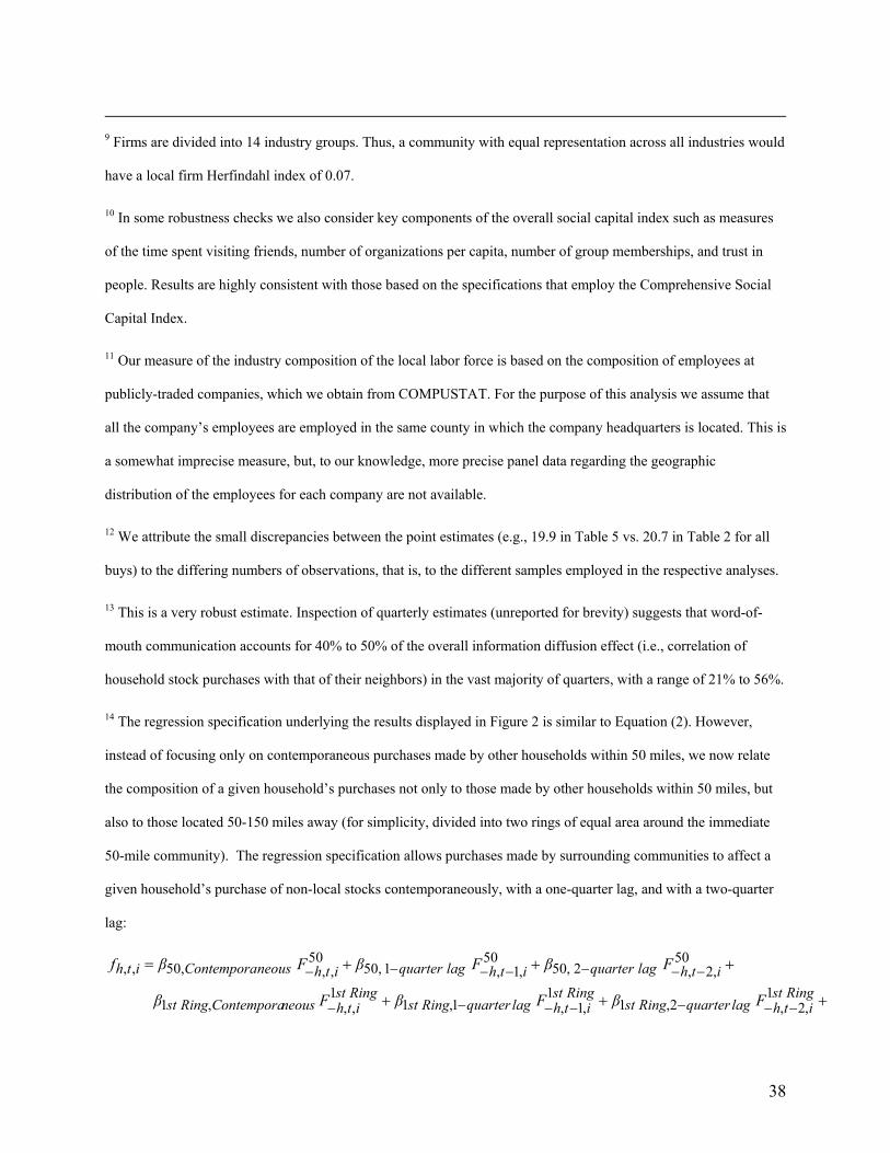
+++= −−−−−−−50

,2,2,5050

,1,1,5050

,,,50,, ithlagquarterithlagquarterithneousContemporaith FFFf βββ

+++ −−−−−−−Ringst

ithlagquarterRingstRingst

ithlagquarterRingstRingstithneousContemporaRingst FFF 1

,2,2,11

,1,1,11

,,,1 βββ

9 Firms are divided into 14 industry groups. Thus, a community with equal representation across all industries would

have a local firm Herfindahl index of 0.07.

10 In some robustness checks we also consider key components of the overall social capital index such as measures

of the time spent visiting friends, number of organizations per capita, number of group memberships, and trust in

people. Results are highly consistent with those based on the specifications that employ the Comprehensive Social

Capital Index.

11 Our measure of the industry composition of the local labor force is based on the composition of employees at

publicly-traded companies, which we obtain from COMPUSTAT. For the purpose of this analysis we assume that

all the company’s employees are employed in the same county in which the company headquarters is located. This is

a somewhat imprecise measure, but, to our knowledge, more precise panel data regarding the geographic

distribution of the employees for each company are not available.

12 We attribute the small discrepancies between the point estimates (e.g., 19.9 in Table 5 vs. 20.7 in Table 2 for all

buys) to the differing numbers of observations, that is, to the different samples employed in the respective analyses.

13 This is a very robust estimate. Inspection of quarterly estimates (unreported for brevity) suggests that word-of-

mouth communication accounts for 40% to 50% of the overall information diffusion effect (i.e., correlation of

household stock purchases with that of their neighbors) in the vast majority of quarters, with a range of 21% to 56%.

14 The regression specification underlying the results displayed in Figure 2 is similar to Equation (2). However,

instead of focusing only on contemporaneous purchases made by other households within 50 miles, we now relate

the composition of a given household’s purchases not only to those made by other households within 50 miles, but

also to those located 50-150 miles away (for simplicity, divided into two rings of equal area around the immediate

50-mile community). The regression specification allows purchases made by surrounding communities to affect a

given household’s purchase of non-local stocks contemporaneously, with a one-quarter lag, and with a two-quarter

lag:

38

+++ −−−−−−−

RingndithlagquarterRingnd

RingndithlagquarterRingnd

RingndithneousContemporaRingnd FFF 2

,2,2,22

,1,1,22

,,,2 βββ

itht i

itit D ,,23

1

14

1,, εγ∑ ∑

= =+ .

39

Table 1

Quarterly Purchases of Stock by Households

# Purchases # Distinct HHsMean Quarterly purchase (in $)

[Median] % Local

1991 36,250 20,366 23,242 [7,113] 16.4

1992 36,270 20,300 23,576 [7,500] 17.0

1993 34,377 18,894 25,150 [7,500] 16.4

1994 28,726 16,307 25,418 [7,388] 17.4

1995 30,299 16,134 38,540 [9,313] 17.8

1996 (Q1-Q3)

25,364 15,483 42,277 [9,725] 17.5

TOTAL 191,286 35,673 28,922 [7,949] 17.1

This table summarizes quarterly household stock purchases at the industry level. Summary statistics are reported annually from 1991 to 1996, as well as for the entire sample period (bottom row of the table). The first column presents the number of household, quarter, industry (h, t, i) combinations in a given year such that household h made at least one purchase in quarter t in industry i. The second column tallies the number of distinct households appearing in the sample in a given year. The third column lists average dollar values of households’ quarterly purchases, where median values are reported in parentheses directly underneath the mean values. The last column breaks down the purchases according to their distance from the household (i.e., whether the firm headquarters is located within 50 miles of the household).

40

Table 2 Information Diffusion for Purchases, Sales, and Positions

Composition of HH Variable ≤ 50 miles R2 # obs.

Panel A: Purchases All Buys

20.7(0.3)

***

0.142

2,678,004

Local Buys (within 50 miles)

119.3(1.2)

***

0.232

568,247

Non-Local Buys (outside 50 miles)

8.4(0.3)

***

0.129

2,337,314

Panel B: Sales All Sells

30.0(0.3)

***

0.123

2,448,838

Local Sells (within 50 miles)

122.4(1.2)

***

0.248

526,273

Non-Local Sells (outside 50 miles)

6.5(0.3)

***

0.104

2,115,722

Panel C: Positions All Positions

36.5(0.3)

***

0.087

8,359,442

Local Positions (within 50 miles)

153.4(0.7)

***

0.143

2,429,728

Non-Local Positions (outside 50 miles)

17.7(0.3)

***

0.072

7,449,582

This table presents the results of fitting the basic information diffusion regression from Equation (2) over the 23 quarters from January of 1991 to October 1996:

itht i

ititithith DFf ,,23

1

14

1,,

50,,,, εγβ ∑ ∑

= =− ++= .

Panel A reports regression results relating the composition of households’ stock purchases across 14 broad industry groups to the composition of their communities’ purchases (the community is defined as all other households within 50 miles). Analogously, Panels B and C present regression results for the composition of sales and positions, respectively. Regressions in all three panels are estimated on subsamples identified by the distance from households to company headquarters (All, Local, and Non-Local). Standard errors, shown in parentheses, allow for heteroskedasticity, as well as correlation of error terms at the household-quarter level. ***, **, * denote significance at the 1 percent, 5 percent, and 10 percent levels, respectively.

41

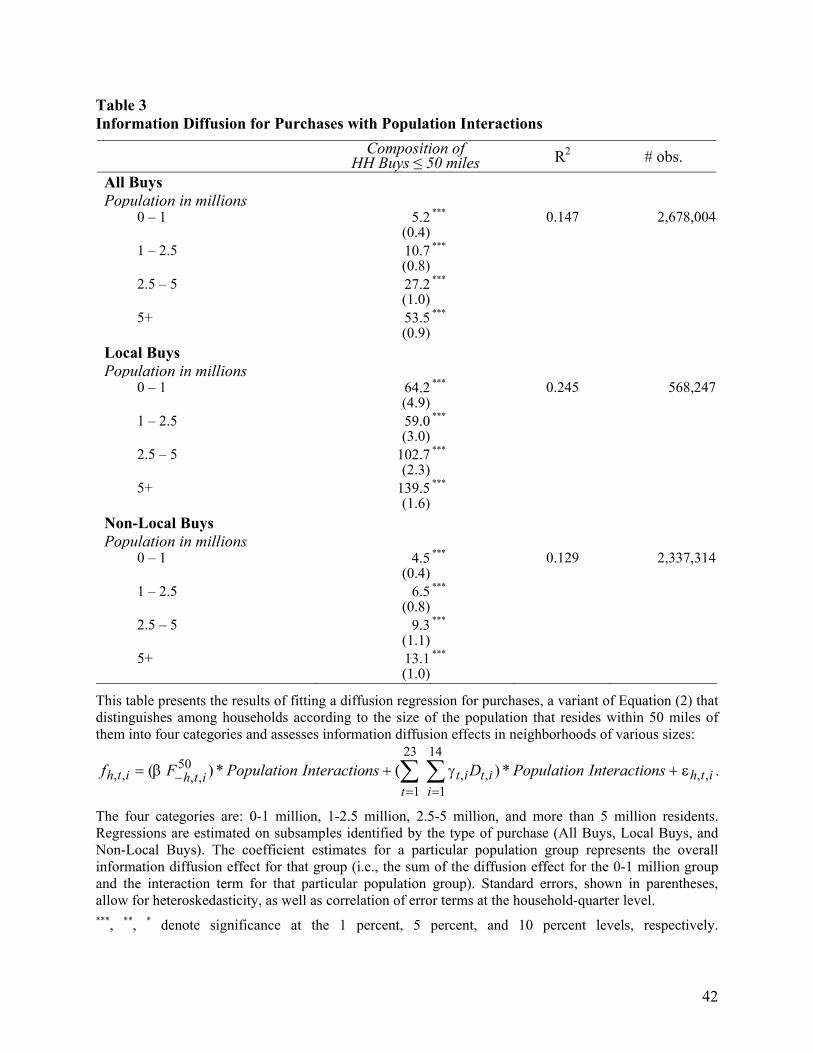
42

Table 3 Information Diffusion for Purchases with Population Interactions

Composition of HH Buys ≤ 50 miles R2 # obs.

All Buys Population in millions 0 – 1

5.2(0.4)

***

0.147

2,678,004

1 – 2.5

10.7(0.8)

***

2.5 – 5

27.2(1.0)

***

5+

53.5(0.9)

***

Local Buys Population in millions 0 – 1

64.2(4.9)

***

0.245 568,247

1 – 2.5

59.0(3.0)

***

2.5 – 5

102.7(2.3)

***

5+

139.5(1.6)

***

Non-Local Buys Population in millions 0 – 1

4.5(0.4)

***

0.129 2,337,314

1 – 2.5

6.5(0.8)

***

2.5 – 5

9.3(1.1)

***

5+

13.1(1.0)

***

***, **, * denote significance at the 1 percent, 5 percent, and 10 percent levels, respectively.

This table presents the results of fitting a diffusion regression for purchases, a variant of Equation (2) that distinguishes among households according to the size of the population that resides within 50 miles of them into four categories and assesses information diffusion effects in neighborhoods of various sizes:

The four categories are: 0-1 million, 1-2.5 million, 2.5-5 million, and more than 5 million residents. Regressions are estimated on subsamples identified by the type of purchase (All Buys, Local Buys, and Non-Local Buys). The coefficient estimates for a particular population group represents the overall information diffusion effect for that group (i.e., the sum of the diffusion effect for the 0-1 million group and the interaction term for that particular population group). Standard errors, shown in parentheses, allow for heteroskedasticity, as well as correlation of error terms at the household-quarter level.

itht i

ititithith nsInteractioPopulationDnsInteractioPopulationFf ,,

23

1

14

1,,

50,,,, *)(*)( ε+γ+β= ∑ ∑

= =− .

Table 4 Information Diffusion, Area Sociability, and Area Population

Population in millions Full Sample 0 – 1 1 – 2.5 2.5 – 5 5+ R2 # obs.

Panel A: All Buys Buys of HHs ≤ 50 miles 14.6

(0.4)***

0.147 2,634,338

Buys of HHs ≤ 50 miles * Sociability Above Median

10.0(0.3)

***

Buys of HHs ≤ 50 miles 5.3(0.6)

***

9.3

(0.8)***

22.5(1.1)

***

42.3(1.0)

***

0.148 2,634,338

Buys of HHs ≤ 50 miles * Sociability Above Median

0.0(0.6)

3.1

(0.7)***

7.4

(0.6)***

9.0

(0.4)***

Panel B: Local Buys Buys of HHs ≤ 50 miles 98.9

(1.4)***

0.236 566,735

Buys of HHs ≤ 50 miles * Sociability Above Median

20.1(0.7)

***

Buys of HHs ≤ 50 miles 63.1(5.6)

***

48.2(3.2)

***

92.1(2.6)

***

117.0(2.1)

***

0.249 566,735

Buys of HHs ≤ 50 miles * Sociability Above Median

0.8(4.6)

20.7(2.3)

***

13.8(1.4)

***

16.8(0.8)

***

Panel C: Non-Local Buys Buys of HHs ≤ 50 miles 6.8

(0.4)***

0.129 2,295,090

Buys of HHs ≤ 50 miles * Sociability Above Median

3.0(0.3)

***

Buys of HHs ≤ 50 miles 4.6(0.6)

***

6.2

(0.9)***

6.1

(1.1)***

8.5

(1.1)***

0.130 2,295,090

Buys of HHs ≤ 50 miles * Sociability Above Median

-0.1(0.6)

0.8

(0.7)

4.8

(0.7)***

3.7

(0.5)***

43

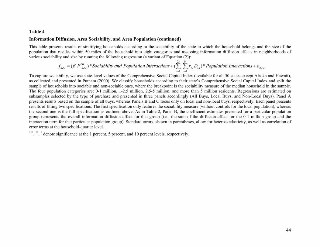
44

Table 4 Information Diffusion, Area Sociability, and Area Population (continued) This table presents results of stratifying households according to the sociability of the state to which the household belongs and the size of the population that resides within 50 miles of the household into eight categories and assessing information diffusion effects in neighborhoods of various sociability and size by running the following regression (a variant of Equation (2)):

itht i

ititithith nsInteractioPopulationDnsInteractioPopulationandySociabilitFf ,,

23

1

14

1,,

50,,,, *)(*)( εγβ ∑ ∑

= =− ++= .

To capture sociability, we use state-level values of the Comprehensive Social Capital Index (available for all 50 states except Alaska and Hawaii), as collected and presented in Putnam (2000). We classify households according to their state’s Comprehensive Social Capital Index and split the sample of households into sociable and non-sociable ones, where the breakpoint is the sociability measure of the median household in the sample. The four population categories are: 0-1 million, 1-2.5 million, 2.5-5 million, and more than 5 million residents. Regressions are estimated on subsamples selected by the type of purchase and presented in three panels accordingly (All Buys, Local Buys, and Non-Local Buys). Panel A presents results based on the sample of all buys, whereas Panels B and C focus only on local and non-local buys, respectively. Each panel presents results of fitting two specifications. The first specification only features the sociability measure (without controls for the local population), whereas the second one is the full specification as outlined above. As in Table 2, Panel B, the coefficient estimates presented for a particular population group represents the overall information diffusion effect for that group (i.e., the sum of the diffusion effect for the 0-1 million group and the interaction term for that particular population group). Standard errors, shown in parentheses, allow for heteroskedasticity, as well as correlation of error terms at the household-quarter level. ***, **, * denote significance at the 1 percent, 5 percent, and 10 percent levels, respectively.

Table 5

Information Diffusion, Correlated Preferences for Industry Allocation, and Structure of Local Economy

Composition of...

Buys Buys of HHs ≤ 50 miles

Positions of HHs ≤ 50 miles

Positions of this HH

Firms ≤ 50 miles

Workers ≤ 50 miles R2 # obs.

Panel A: All Households

All

19.9(0.4)

*** 0.134 1,786,666

All

9.8(0.4)

*** 16.5(0.5)

*** 32.5(0.2)

*** 0.204 1,786,666

All

17.4(0.4)

*** 4.8(0.3)

*** 4.0 (0.3)

*** 0.135 1,786,666

All

9.0(0.4)

*** 14.5(0.6)

*** 32.4(0.2)

*** 1.9(0.3)

*** 2.7 (0.3)

*** 0.204 1,786,666

All (HH-industry Fixed Effects)

3.6(0.5)

***

0.323

1,786,666

Local

128.9(1.7)

*** 0.249 265,509

Local

43.6(1.7)

*** 58.8(2.3)

*** 47.5(0.5)

*** 0.417 265,509

Local

85.1(1.8)

*** 46.9(1.4)

*** 14.2 (1.3)

*** 0.276 265,509

Local

36.8(1.7)

*** 40.1(2.4)

*** 46.2(0.5)

*** 18.1(1.2)

*** 5.6 (1.1)

*** 0.421 265,509

Local (HH-industry Fixed Effects)

17.7(2.5)

***

0.577

265,509

Non-Local

7.4(0.4)

*** 0.121 1,510,390

Non-Local

3.7(0.4)

*** 7.2(0.6)

*** 31.2(0.2)

*** 0.186 1,510,390

Non-Local 7.0(0.4)

*** 0.7(0.3)

*** 1.0 ***

(0.3) 0.121 1,510,390

Non-Local 3.6(0.4)

*** 7.0(0.6)

*** 31.2(0.2)

*** -0.1(0.3)

0.8 (0.3)

*** 0.186 1,510,390

Non-Local (HH-industry Fixed Effects)

2.4(0.5)

***

0.305

1,510,390

45

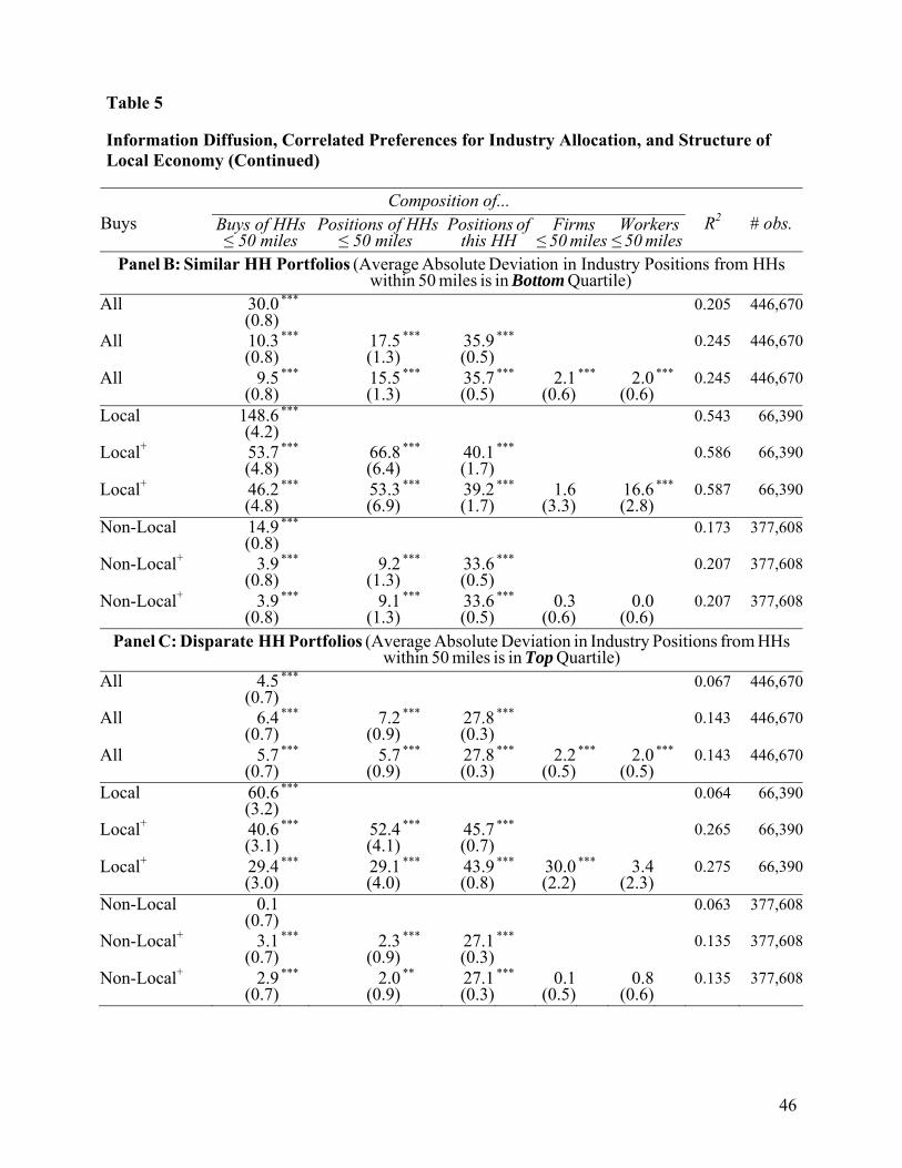
Table 5

Information Diffusion, Correlated Preferences for Industry Allocation, and Structure of Local Economy (Continued)

Composition of... Buys Buys of HHs

≤ 50 miles Positions of HHs

≤ 50 miles Positions of

this HH Firms ≤ 50 miles

Workers ≤ 50 miles

R2 # obs.

Panel B: Similar HH Portfolios (Average Absolute Deviation in Industry Positions from HHs within 50 miles is in Bottom Quartile) All

30.0 (0.8)

*** 0.205 446,670

All

10.3 (0.8)

*** 17.5(1.3)

*** 35.9(0.5)

*** 0.245 446,670

All

9.5 (0.8)

*** 15.5(1.3)

*** 35.7(0.5)

*** 2.1(0.6)

*** 2.0 ***

(0.6) 0.245 446,670

Local

148.6 (4.2)

*** 0.543 66,390

Local+

53.7 (4.8)

*** 66.8(6.4)

*** 40.1(1.7)

*** 0.586 66,390

Local+

46.2 (4.8)

*** 53.3(6.9)

*** 39.2(1.7)

*** 1.6(3.3)

16.6 (2.8)

*** 0.587 66,390

Non-Local

14.9 (0.8)

*** 0.173 377,608

Non-Local+

3.9

(0.8) *** 9.2

(1.3)*** 33.6

(0.5)*** 0.207 377,608

Non-Local+

3.9

(0.8) *** 9.1

(1.3)*** 33.6

(0.5)*** 0.3

(0.6) 0.0

(0.6) 0.207 377,608

Panel C: Disparate HH Portfolios (Average Absolute Deviation in Industry Positions from HHs within 50 miles is in Top Quartile) All

4.5 (0.7)

*** 0.067 446,670

All

6.4 (0.7)

*** 7.2(0.9)

*** 27.8(0.3)

*** 0.143 446,670

All

5.7 (0.7)

*** 5.7(0.9)

*** 27.8(0.3)

*** 2.2(0.5)

*** 2.0 (0.5)

*** 0.143 446,670

Local

60.6 (3.2)

*** 0.064 66,390

Local+

40.6 (3.1)

*** 52.4(4.1)

*** 45.7(0.7)

*** 0.265 66,390

Local+

29.4 (3.0)

*** 29.1(4.0)

*** 43.9(0.8)

*** 30.0(2.2)

*** 3.4 (2.3)

0.275 66,390

Non-Local

0.1 (0.7)

0.063 377,608

Non-Local+

3.1

(0.7) *** 2.3

(0.9)*** 27.1

(0.3)*** 0.135 377,608

Non-Local+

2.9

(0.7) *** 2.0

(0.9)** 27.1

(0.3)*** 0.1

(0.5) 0.8

(0.6) 0.135 377,608

46

Table 5

Information Diffusion, Correlated Preferences for Industry Allocation, and Structure of Local Economy (Continued)

This table presents results of assessing the contribution of word-of-mouth effects to the overall information diffusion effect (i.e., correlation of household stock purchases with that of their neighbors). Accordingly, we regress households’ industry-level purchases on neighbors’ purchases, variables capturing correlated preferences for industry allocation, variables capturing the structure of the local economy, and 322 industry-time dummy variables (a variant of Equation (2)). Two variables for each (h, t) observation are used to capture correlated preferences. First, we define the industry composition of stock positions of neighboring households (excluding household h itself) at the end of quarter t–1. Second, we define the industry composition of stock positions of the household itself at the end of quarter t–1. To capture the impact of the structure of the local economy, for each (h, t, i) observation we define two variables: the fraction of market value of companies local to household h in quarter t in industry i and the fraction of the labor force local to household h in quarter t employed in industry i. In this framework, estimates of β are conservative lower bounds on the contribution of word-of-mouth effects to the overall information diffusion effect. Panel A has three sections, containing estimates for all buys, local buys, and non-local buys, respectively. Within each section, we first show the baseline result (i.e., Equation (2)). The following row in each section shows the results with the two additional independent variables that seek to capture preferences for industry allocation. The third row in each section of Panel A includes the variables that capture the structure of the local economy. The fourth row in each section features the results of relating the industry composition of a household’s investments to both preferences (the neighborhood’s and own) and the structure of the local economy. The final analysis, reported in the fifth row in each section, seeks to capture differences among households along unobservable characteristics by running the baseline regression from Equation (2) with the inclusion of household-industry-level fixed effects. Panels B and C show results of replicating the key analyses from Panel A on two subsamples of households. Specifically, we sort households into two types according to the extent to which their household portfolio allocations at the industry level conform to those of their neighbors; the metric we use is the average absolute deviation in industry portfolio shares between a household and its neighborhood. Standard errors, shown in parentheses, allow for heteroskedasticity, as well as correlation of error terms at the household-quarter level.

***, **, * denote significance at the 1 percent, 5 percent, and 10 percent levels, respectively.

+ denotes that the difference in coefficients across the similar and disparate samples is not significant at the one percent level.

47

48

00-50 50-71 71-87 87-100 100-112 112-122 122-132 132-141 141-150

1

2

3

4

5

6

7

8(%)

0

2

4

6

8

10

12

14

16

18

20Panel A: All Buys (%)

0-50 50-71 71-87 87-100 100-112 112-122 122-132 132-141 141-150 radius [miles]

Panel B: Local Buys

20

40

60

80

100

120(%)

00-50 50-71 71-87 87-100 100-112 112-122 122-132 132-141 141-150 radius [miles]

Panel C: Non-Local Buys

radius [miles]

Figure 1: Dissipation of Information Diffusion. The figure illustrates dissipation of information diffusion effects with distance from the household. Regions surrounding the household at increasingly larger distances have the same geographic area (502 π = 7,854 square miles). The regression specification is similar to Equation (2), except, instead of having one information diffusion regressor, the specification now has nine–one for each geographic area.

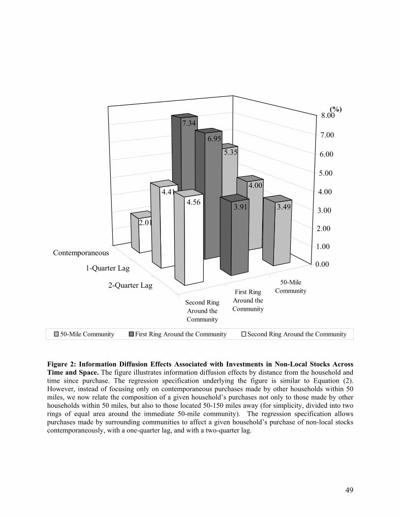
2-Quarter Lag

1-Quarter Lag

Contemporaneous

50-MileCommunityFirst Ring

Around theCommunity

Second RingAround theCommunity

5.35

4.00

3.49

7.34

6.95

3.91

2.01

4.414.56

0.00

1.00

2.00

3.00

4.00

5.00

6.00

7.00

8.00

50-Mile Community First Ring Around the Community Second Ring Around the Community

(%)

Figure 2: Information Diffusion Effects Associated with Investments in Non-Local Stocks Across Time and Space. The figure illustrates information diffusion effects by distance from the household and time since purchase. The regression specification underlying the figure is similar to Equation (2). However, instead of focusing only on contemporaneous purchases made by other households within 50 miles, we now relate the composition of a given household’s purchases not only to those made by other households within 50 miles, but also to those located 50-150 miles away (for simplicity, divided into two rings of equal area around the immediate 50-mile community). The regression specification allows purchases made by surrounding communities to affect a given household’s purchase of non-local stocks contemporaneously, with a one-quarter lag, and with a two-quarter lag.

49