Information and Bargaining through Agents: Experimental

Evidence from Mexico’s Labor Courts

Joyce Sadka, Enrique Seira, and Christopher Woodruff ∗

October 26, 2020

Abstract

Well-functioning courts are essential for the health of both financial and real economies.

Courts function poorly in most lower-income countries, but the root causes of poor perfor-

mance are not well understood. We use a field experiment with ongoing cases to analyze

sources of dysfunction in Mexico’s largest labor court. Providing the parties with person-

alized outcome predictions doubles settlement rates and reduces average case duration, but

only when the worker is present to receive the information. An intervention before plaintiffs

contact a lawyer increases pre-suit settlement. The experiment illuminates agency issues

among plaintiffs with private lawyers. For most workers, the treatment appears to improve

welfare, as measured by discounted payouts and ability to pay bills.

Keywords: labor courts, settlement, overconfidence, statistical information

JEL Codes: K31, K41, K42, J52, J83

∗

Sadka: ITAM, jsadka@itam.mx; Seira: ITAM, enrique.seira@itam.mx; Woodruff: University of Oxford, christo-pher.woodruff@qeh.ox.ac.uk. Acknowledgements: We would like to thank Sebastian Garcia, Andrea Fernandez,Sergio Lopez-Araiza, Enrique Miranda, Isaac Meza, Diana Roman, and Monica Zamudio for superhuman re-search assistance, Vince Crawford, Jonas Hjort and Bentley MacLeod for helpful discussions, and seminar andconference participants at Cambridge, Columbia, Toulouse, ITAM, Monash, NYU - Abu Dhabi, Oxford, Tin-bergen, MIT/Harvard, George Mason, Maryland the Latin American Workshop on Law and Economics, andthe American Law and Economics Association for comments. All errors are ours. We acknowledge financialsupport from the Government Partnership Initiative of the Abdul-Latif Jameel Poverty Action Lab (JPAL) atthe Massachusetts Institute of Technology, the Economic Development and Institutions program funded by theUK government through UK Aid, and the Asociacion Mexicana de Cultura. We also acknowledge crucial insti-tutional, operational, and human resource support from the Mexico City Labor Court and its president, DarleneRojas Olvera. The research reported in the paper was carried out with the approval of the ITAM InstitutionalReview Board. The trial registration number is AEARCTR-0002339.

1

1 Introduction

Well-functioning courts underpin markets and constrain private power in developed economies,

but courts function poorly in most developing countries. Outcomes are unpredictable, par-

ties are misinformed, and inefficient processes lead to slow decisions and large case backlogs

(Djankov et al. (2003)). In addition to raising concerns for justice, poorly functioning courts

undermine both the financial (Ponticelli and Alencar (2016)) and real (Boehm and Oberfield

(2020); Chemin (2020)) economies. The effects of poorly functioning courts are increasingly

well documented, most convincingly through studies analyzing changes following the creation

of new institutions providing legal services for specific activities (Visaria (2009); Lichand and

Soares (2014)). However, as Boehm and Oberfield (2020) note, even “Newly created courts

tend to...accumulate backlogs over time” (p. 2009). Thus, while the existing literature provides

evidence on the importance of well-functioning legal institutions, it is much less informative on

how to improve the performance of existing institutions, or how to ensure the continued high

performance of the new institutions. This is due in part to a lack of rigorous empirical work

aimed at understanding the micro-analytics of court proceedings, and a particular paucity of

randomized experiments in courts (Greiner and Matthews (2016)).

To illuminate the causes of dysfunction in courts, we conduct a randomized experiment with

active cases in the Mexico City Labor Court (MCLC). The MCLC is responsible for enforcing

labor law for all private employers located in Mexico City. Most cases involve workers who

claim to have been involuntarily separated from their jobs by employers who then failed to make

severance payments to the workers as required under the labor law. Each year the court receives

more than 35,000 filings, but resolves less than 30,000 cases. The MCLCs growing case backlog

stems in part from its settlement rates, which are low in comparison to those of similar courts in

other countries. Taking a cue from the literature on bargaining under asymmetric information,

our experimental treatment provides parties with case-specific predictive outcomes, generated

from machine-learning models using data from 5,000 concluded cases. We use the experiment

to understand how the relationship between plaintiffs and their lawyers affects the settlement

and progression of their cases through the court.

Mexico’s job-insurance system is based on severance payments made directly by firms to

dismissed workers. On paper, the law is straightforward and very favorable for Mexican work-

ers. Dismissed workers are entitled to a minimum severance payments of 90 days’ wages and,

2

depending on circumstances, substantially more. Payments must be made even if the dismissal

is due to loss of business by the firm. However, while the law itself is generous, the framework for

enforcing the law disadvantages workers for at least three reasons. First, workers and firms are

often informal (Kumler, Verhoogen and Frias (2020)). Wages are paid in part or entirely in cash

and there is no formal written contract. In these circumstances, dismissed workers may find it

difficult to prove wage levels or even the existence of the labor relationship itself. Second, at the

time of hiring, firms often take actions that undermine the workers subsequent claim of unfair

dismissal. For example, firms may require the worker to sign an undated letter of resignation

as a condition of hiring. Third, while the payments from the unemployment insurance systems

used in most countries are made by the government, payments in Mexico are made directly

from the firm to the worker. Workers who win a judgment often face challenges in recover-

ing payments ordered by the court from their former employers. The firms can avoid making

payments through a combination of transferring assets to other entities, firm bankruptcy, and

bribes. With the threat of avoiding payment, firms often negotiate much lower payments even

after the court rules against them. Indeed, administrative records show that that, more than

half of the time, workers winning a court judgment are unable to recover anything.

We demonstrate the relevance of these disadvantages by using the historical case files to

document a set of stylized facts about the functioning of the court. First, the historical data

show that plaintiffs receive, on average, only around half of the minimum 90-day compensation

called for in the law. Second, although the law stipulates that suits should be adjudicated within

three months, more than a third of the cases filed in the court between 2009 and 2012 remained

unresolved in early 2016. The backlog of cases is driven in part by low settlement rates: around

55 percent of cases are settled in Mexico, compared with 80 to 90 percent in higher-income

countries. Third, parties are overconfident: the sum of the two parties’ probabilities of winning

far exceeds 100 percent, and both the probability of winning and the expected size of the award

are optimistic, particularly on the plaintiff’s side, relative to predictions based on historical

cases. Fourth, plaintiffs have little knowledge of their legal entitlements. Moreover, even those

represented by private lawyers are surprisingly uninformed about the contents of their own

lawsuits. Finally, we show that although private lawyers file much larger claims, they do not

recover more than public lawyers. After accounting for fees, private lawyers actually recover

less than public lawyers.

Working with the court, we conduct an experiment in three phases, which differ in the point

3

at which we intervene in the process. In phase 1, we intervene in ongoing cases at any point

in the life of the lawsuit. We find that the information treatment increases settlement on the

day of treatment by 75 percent, and that settlements are more frequent in cases that are early

in the process. In phase 2, given the potential of earlier interventions to be more effective, we

intervene in the first hearing of each case. Although there are more settlements at the first

hearing, we find that the effect of the information treatment is of very similar magnitude. In

both the first and second phases, we find that the treatment is effective only when the employee

is present at the hearing, and only in cases where the employee is represented by a private

lawyer.1 Administrative data from 42 months after treatment indicate that an additional 38

percent of the cases in both the control and treatment groups are settled after the day of our

intervention; however, the treatment effect and the relevance of the employee receiving the

treatment directly remain constant over that time. The importance of the employee’s presence

for even long-run outcomes suggests that lawyers do not convey the information to their clients.

The persistence in the treatment effect indicates that the intervention led to settlement of cases

that would not have been settled otherwise. Perhaps most importantly, data on case outcomes

from phase 1 and 2 show that the increase in settlements improves the outcomes for the typical

plaintiff. These patterns suggest that case trajectories are affected by lawyer-plaintiff agency

issues. Given this, in phase 3, we work with a sample of recently dismissed workers who come

to the court seeking information about their rights before they contract with a lawyer and

file a case. The treatment providing predicted case outcomes is again effective in increasing

settlement, this time before a case is filed.

The results of the three experiments suggest that informational asymmetries between the

worker and her lawyer are one underlying cause of malfunctioning courts. A majority of plaintiffs

earn below the median wage and have modest levels of schooling; more than 80 percent are using

the court for the first time. Survey responses indicate that 38 percent of plaintiffs found their

lawyer on the sidewalk outside the court building, where many lower-quality lawyers find clients.

The workers are wildly overconfident about their chances of winning their lawsuit. We show

analytically that the incentives of the lawyers, who have information advantages, do not always

align with those of their clients even though private lawyers in the MCLC cases almost always

receive a share of the award collected by their plaintiffs. Differences in the ability to diversify

1Both the choice of lawyer and the presence of the employee at the hearing may be endogenous to outcomes.However, the treatment is orthogonal to either. We discuss this issue in more detail below.

4

risk and discount rates lead to very different preferences over settlement options between the

plaintiffs and their lawyers. Lawyers also charge an initial fee that is generous relative to the

time required to file a suit, giving them incentives to file cases even when they have little

prospect of winning.

By 2020, almost 90 percent of both treatment and control cases in the first two phases were

resolved. This allows us to examine how treatment affects the welfare of plaintiffs. Relative to

the control group, those in the treatment group are 6.7 percent more likely to have settled, 7.3

percent less likely to have lost a judgment, and 0.4 percent less likely to have won a judgment.

The additional settlements come mainly from cases with modest recovery amounts. When we

compare the net present value of the amount collected by plaintiffs in the treatment and control

groups, we find that the treatments improved the outcomes for the typical plaintiff. Though

making a precise statement about plaintiff welfare is difficult for reasons we discuss in Section

7, surveys two months after treatment show that treated workers in Phase 3 are 7 percent less

likely to report not having enough food to eat or being unable to pay for basic services; reported

happiness is insignificantly higher with treatment.

Experiments in courts are uncommon. Greiner and Matthews (2016) review the small

number of randomized evaluations in the US legal system, finding 50 studies conducted between

1963 and 2015. Most of these examine mediation and alternative dispute resolution, though

a handful evaluate programs that affect the use of lawyers. There are likewise very few legal

experiments in low-income countries.2 As a result, there is little credible evidence on the source

of delays and the effect of differences in rules and organizational structure. Indeed, given

the scarcity of diagnostic information about courts in developing countries, the stylized facts we

derive from extensive administrative records contribute to the literature on courts as institutions

for development.

The paper also contributes to the literature on experts and moral hazard. The most closely

related paper in this literature is Anagol, Cole and Sarkar (2017), who conduct an audit ex-

periment in the Indian life insurance market. They show that agents use their informational

2Two notable exceptions are Aberra and Chemin (2019), who provide access to lawyers to randomly selectedplaintiffs in cases involving land disputes, showing that legal assistance leads to greater investment in land held bythe plaintiffs; and Sandefur and Siddiqi (2015), who provide access to paralegals that lower the cost of accessingthe formal legal system in Senegal. They find that access to the formal legal system is particularly valuable forthose most likely to be disadvantaged in the customary legal system – for example, women who are suing men.Kondylis and Stein (2018) use an abrupt change in procedural rules rolled out across six civil courts in Senegalto identify the effect of the reforms; the authors find that the new regulation resulted in in faster pre-trial phasesof cases.

5

advantage to induce clients to make decisions that are favorable to the agents’ interest. There

is much more extensive observational evidence that agents take advantage of superior informa-

tion in diverse settings: Schneider (2012) in Canadian auto repair shops; Emons (1997) among

doctors in Switzerland; and Levitt and Syverson (2008) among real estate agents in the US.3

A third related literature is that of bargaining in the field. Courts are a disciplining device

for a bargaining game between the parties to the case. The canonical Rubinstein (1982) bargain-

ing framework shows that bargaining outcomes are immediate and efficient where information is

complete, delays are costly, and parties bargain by making alternating offers. However, the ef-

ficiency result breaks down if parties have asymmetric information (Myerson and Satterthwaite

(1983)). Bargaining may also break down or be delayed if parties are overly optimistic.4 Our

data indicate that both misinformation and excessive optimism are characteristics in the MCLC

cases. Most of the relevant bargaining literature constructs a game between two parties, but

court cases typically involve four parties: the plaintiff, the defendant and the lawyers represent-

ing either side. This distinction is relevant if agency is important. Note that, theoretically, the

addition of lawyers may result in either more- or less-efficient outcomes. Gilson and Mnookin

(1994) model court cases as prisoners dilemmas in which the parties play once and the lawyers

play repeatedly. As such, the lawyers may cooperate when the players would not, generating

more-efficient outcomes. Ashenfelter and Dahl (2012) examine data from arbitration cases in-

volving emergency services unions and municipalities in New Jersey. In a context in which the

parties sometimes represent themselves and sometimes are represented by lawyers, they show

that lawyer-agents provide positive benefits to the party they represent.

Finally, we contribute to the literature on the effects of information provision and decision

making. Information has been shown to improve decision making in wide range of other con-

texts: in the functioning of private markets (Andrabi, Das and Khwaja (2017); Belot, Kircher

and Muller (2019)), in schooling decisions (Jensen (2010); Dizon-Ross (2019)), and in political

institutions (Chong et al. (2015); Reinikka and Svensson (2011)). Our results focus on courts

and suggest that it is important that the information be conveyed directly to the party affected

by the decisions.

3Hubbard (1998) and Hubbard (2000) suggest that reputation is effective in controlling agency in the auto-mobile emissions testing market in California. However, in labor courts, the development of reputations amonglawyers is limited both because plaintiffs typically use the court only once, and because the plaintiffs seldomconnect with one another.

4See Yildiz (2011) for a review of the related theory. Overoptimism may also reflect self-serving bias (Babcockand Loewenstein (1997)).

6

The rest of the paper proceeds as follows: We begin by describing the context and the

Mexican labor law in Section 2. We then detail the data from both administrative records

and surveys of litigants and lawyers in Section 3. Section 4 uses those data to describe a set

of stylized facts that motivate our experiment. Section 5 describes the experimental protocol

and Section 6 the results. We discuss the welfare implications of the results in Section 7 and

conclude in Section 8.

2 The Context

Gerard and Naritomi (2019) shows that while unemployment insurance is the most common

job-displacement insurance system in higher-income countries, severance payment programs are

the norm in Africa, Asia and Latin America. Mexico’s system of severance payments fits this

pattern. Mexican workers dismissed from their job for almost any reason are entitled to 90

days’ wages and often substantially more, with payments made directly by firms to workers.

Severance payment provisions in the private sector are governed by federal labor law in Mexico,

with adjudication of disputes in most industries assigned to state-level labor courts.5 We work

with the Mexico City Labor Court, the state court serving Mexico City. Each year, the MCLC

receives more than 35,000 new cases and concludes fewer than 30,000 cases. Its portfolio of

100,000 active cases is therefore not only large but growing.

Lawsuits filed by dismissed workers claiming they have not received severance payments

owed to them account for over 95 percent of MCLC filings. These cases are assigned to one

of 20 “subcourts” according to the industry in which the plaintiff was employed. In the first

phase of the project, we worked with Subcourt 7, which deals mainly with firms in the retail

automotive and transport services industries. In phase 2, we expanded to four additional sub-

courts specializing in industries such as private education, security, restaurants, retail banking,

large department stores, and medical services. In phase 3, we worked with dismissed workers

approaching the court who might ultimately file a case assigned to any of the 20 subcourts.

We describe the Mexican Labor Law and the court procedures in more detail in Appendix

A. Plaintiffs may be represented by either private or public lawyers. Private lawyers typically

charge around 2000 MXP (USD 100) to file a case, and then receive 30 percent of any amount

recovered by the worker. Lawyers from the Public Attorney’s office are paid a fixed wage and

5Disputes in a few “strategic” industries named in the Mexican constitution - oil and gas, pharmaceuticalsand auto manufacturing, for example are handled by a federal-level labor court.

7

do not charge their clients for services. Employers most often respond to a suit in one of three

ways: denying the existence of a labor relationship, offering reinstatement, or claiming the

worker resigned voluntarily and producing a letter of resignation signed by the employee.6 High

levels of informality make it more difficult for plaintiffs to prove employment relationships and

easier for employers to hide assets. These strategies decrease the likelihood that workers who

win a judgment or collect the compensation the court awards them.

The parties reach a settlement in around 55 percent of the cases. Cases that settle usually

do so within a year of filing. In the absence of settlement, cases typically involve at least

six to eight hearings spread over several years. The hearings are conducted by administrative

assistants to the judge, but the judge of the subcourt makes all rulings, based on the written

record prepared by the assistants. Judgments within three years of filing are rare. Even when

workers win their suit, a large proportion of firms do not pay the judgment voluntarily. The

plaintiffs must then pursue seizure of assets through officers of the court. Firms have many

ways of avoiding asset seizure, for example by declaring bankruptcy or transferring assets to

another entity. In more than half the historical cases we code, workers winning the suit are not

able to collect any payment.

The challenges for workers arise from informality on several levels. Even workers employed

formally and registered with the Mexican Social Security Administration are often paid part

of their wages off-books and in cash (Kumler, Verhoogen and Frias (2020)). Workers will

generally only be able to recover based on the formal part of their wages. Firm assets are also

unregistered. Hence, the court cannot place liens on assets at the time of its ruling. Finally, the

process of notification is hampered by corruption at all stages (Aldeco Leo, Kaplan and Sadka

(2014)). Corruption is likely to be a particular issue at the asset-seizure stage, when the gain

from avoiding notification is clearest for the firms.

3 Data

We use both administrative records and survey data. We describe these data briefly here,

and in more detail in Appendix A. Through an agreement with the court, we had access to

the experimental case files and all of the historical case files from the court. The case files

register all the legally relevant information in the lawsuit. Given the scarcity of evidence on the

6In a large range of low to mid-level jobs, entering employees are obliged to sign a letter of resignation (or a”blank letter”) in advance. After firing, the firm adds a date to the letter.

8

functioning of courts, we view the construction of this data itself as a contribution of the paper.

We conducted the first phase of the experiment in Subcourt 7 between March and May,

2016 and the second phase in Subcourts 2, 7, 9, 11, and 16 between October 2016 and February

2017. In Phases 1 and 2, we intervened in case hearings where both parties had been notified

and were therefore obligated to attend the hearing. We conducted Phase 3 between May 2017

and August 2018 with a sample of dismissed workers who had not yet filed a case. In all three

phases, we carried out very brief surveys of the plaintiffs and lawyers when they were present,

though in Phase 2 the survey was very limited for logistical reasons.

3.1 Administrative data

Historical cases: We began by digitizing the historical case file data with the goal of building

predictive models of case outcomes, as we describe below. Given the duration of the average

lawsuit, we chose to focus on cases filed in 2011, the earliest year for which the court had digital

(pdf) records of all initial case filings. For phase 1, we digitized 2,158 lawsuits filed in 2011 or

2012, assigned to Subcourt 7, and concluded by December 2015. Only 55 of those cases were

concluded by a decision of the judge. In order to increase the sample of cases concluded by the

judge’s decision, we reached back to lawsuits filed in Subcourt 7 in 2009 and 2010, identifying

241 additional case files concluded by a judge’s decision. Together with the 2011 and 2012 cases,

we use these to calibrate the likelihood of winning and amount collected at trial.

For the second phase of the experiment, we used data from 1,000 concluded cases in each

of the five participating subcourts. We again selected cases filed in 2011 and concluded by

December 2015. We used all such cases from Subcourt 7, and a random sample of approximately

1,000 cases in each of Subcourts 2, 9, 11, and 16. Thus, the calculator for Phase 2 was calibrated

with historical data covering 5005 cases, all filed in 2011 and concluded by December 2015.7

Because we often intervened in the first hearing, the predictive model could only use in-

formation included in the initial filing. From the case filing, we capture the amount claimed

by the plaintiff, the date of the lawsuit, whether the lawyer is public or private, the worker’s

gender, age, daily wage, tenure at the firm, and weekly hours worked. The variables are defined

in Table A.1 in Appendix A. The basic formula for severance payment in the law is in large

part a function of the wage, tenure and hours worked.

7For phase 1, the calculator used the full set 2,158 cases filed in 2011 and 2012 in Subcourt 7. We also includethe 2012 cases from Subcourt 7 in the descriptive data we present in the paper.

9

We also record the outcome of the suit and the termination date. Cases end in one of five

ways: being dropped by the plaintiff, expiring due to lack of activity, a judge’s ruling with no

collection, a judge’s ruling with a positive collection, or settlement between the parties. We

record the amount recovered by the worker at the end of the proceedings. The majority of the

cases with positive recoveries end in settlement. These are essentially always recorded at the

court, in order to assure that the plaintiff does not continue to pursue the case. For cases ending

in judgments in favor of the plaintiff, the details of the judge’s decision are sometimes complex

and somewhat opaque and hence difficult to code. Therefore, we did not capture the details of

the decision in the dataset. Note that the amount the plaintiff recovers is often different from

the amount awarded by the judge for three reasons: first, the law provides that if the judgment

is not enforced immediately, additional lost wages may be added to the award; second, the

parties may reach a post-judgment settlement, with the worker accepting a lower payment to

avoid the high costs of enforcing payment; and third, the worker may be unable to collect the

judgment found by the court, for example because the firm may have no assets that can be

seized by the time the judgment is enforced. We show below that in the experimental cases

where the plaintiff won a judgment and collected a positive amount, the plaintiff collected only

52 percent of the estimated reward.

In addition to providing the raw material for the prediction calculator, the historical data

allow us to construct a set of stylized facts about the functioning of the court. We discuss

what the data show with regard to trial length, frequency of settlement, amount collected, the

fraction of plaintiffs collecting awards, and so forth, in the next section.

Administrative data for ongoing cases: We code the initial case file data from all of the on-

going lawsuits involved in Phases 1 and 2 of the experiment. We use these data, combined with

the predictive model developed with the historical data, to predict the outcome of the lawsuit.

We also use the administrative records to determine who attended the hearing on the day of

the experiment, whether the lawsuit ended on that day through a settlement, and the amount

of money recorded for the settlement. We then repeat the data collection in 2020 around 42

months after the start of each phase of the experiment. Administrative records from late 2019

also allow us to see which of the Phase 3 workers sued or settled. As we noted, settlements are

generally registered in court files even for cases that settle out of court, because this is the only

way the firm can ensure that the employee does not continue to pursue the case.

10

3.2 Survey Data

We conducted surveys with parties involved in the experiment in all three phases. In Phases 1

and 2, these were short surveys at the hearing on the day of the experiment. We interviewed

the defendant’s lawyer and either the plaintiff, if she was present at the hearing, or her attorney

if she was not.8 The survey was conducted before parties were aware of their treatment status.

We asked about knowledge of the case file and the relevant law, expected case outcomes, and,

where the plaintiff was present, demographic characteristics of the plaintiff.

In Phase 3, our sample is dismissed workers approaching the court in search of information.

Our survey in this phase collected demographic data similar to Phases 1 and 2, but we also

collected enough information about the worker’s employment to be able to use the calculator

to make predictions on the worker’s own case outcomes. In the first two phases, the relevant

employment data came from the case file itself, but in Phase 3, the workers had not yet filed a

case. In Phase 3, we also conducted telephone follow-up surveys two weeks and two months after

the initial contact. The follow-up surveys recorded actions taken after our initial interaction, and

elicited updated beliefs about case outcomes. For example, we asked workers if they had talked

to a lawyer, and if so, how they had found the lawyer(s). We also asked whether they had filed

a suit, settled, or decided not to pursue any claim, and collected a measure of life satisfaction

and difficulty in paying bills. We conducted at least one of the two telephone surveys with 89

percent of the sample. Survey questions and response rates from all three phases are discussed

in more detail in Appendix A.

Table 2 shows summary statistics of the cases for each of the three phases of the experiment.

We use the administrative data for the first two phases and the survey data from Phase 3. Table

A.2 in Appendix A summarizes data from the plaintiff surveys. We find that 58 percent of

plaintiffs had at most lower secondary schooling. Plaintiffs with public lawyers were more likely

to attend the hearing: 29 percent of workers present at Phase 1 and 2 hearings had a public

lawyer, while only 10 percent of the case files in the experiment had a public lawyer. Of those

workers who showed up and had a private lawyer, most (nearly 82 percent) said their agreement

called for paying their lawyer a fraction of any award (30 percent, on average). Only 7.6 percent

were currently employed, and for those not currently working who were searching for a job, the

8Lawyers for the plaintiff and defendant were almost always present, but the plaintiff was present only 18percent of the time, and the defendant only 1.4 percent of the time. In the interest of time, we surveyed onlyone individual from each side of the case. At least one party completed the baseline survey in 71 percent of thecases. Survey compliance rates are detailed in Table A.3 in Appendix A.

11

average reported likelihood of finding a job in the next three months was 58 percent.

3.3 Construction of the calculator

In the experiment, we provide personalized predictions on important case outcomes to a subset

of plaintiffs and defendants. We developed simple, parsimonious, predictive models using the

historical case records. We considered several machine learning models, including boosting,

random forest, and regularization methods (e.g., ridge), along with OLS and logit. The con-

struction of the calculator is described in detail in Appendix A, but we summarize the main

points here. As we noted, the calculator in Phase 1 was developed using 2,158 cases from Sub-

court 7 and the calculator used in Phases 2 and 3 used 5,005 cases from the five participating

subcourts. The information we provided to the parties also changes somewhat in each phase,

as we describe below.

Our goal was to provide predictions on the expected amount collected by the plaintiff, the

duration of the case, and the probability the case ends by being dropped, expiring, judgment

with zero recovery, judgment with positive recovery, or settlement. The main explanatory

variables were all taken from the initial case filing: daily salary, hours worked per week, tenure

at the firm, gender of the plaintiff, type of lawyer, whether or not the worker was registered

with Social Security, if s/he was employed in a position of high trust (an ‘at-will’ worker), the

specific claims in the case (reinstatement, overtime, back pay, vacation pay, Christmas bonus,

statutory profit sharing, severance pay) and the industry of the firm. We used 70 percent of

the data to fit the models and the remaining 30 percent for testing. For each outcome, we

used cross-validation to choose the model and variables with the best fit on the testing sample,

measured by the correlation between predicted and actual values. Tables A.5 & A.6 in Appendix

A present goodness of fit measures for all the models and highlight those we selected.

The models allow us to produce individualized predictions that we shared with parties

present at the hearing in cases randomized into the calculator treatment. Figure 4 displays the

template we used in Phase 1. The template shows the minimum legal entitlement based on the

law if the plaintiff were to win on the issue of unfair dismissal and the probability the case ends

in each of the five possible endings. For each of these five endings, we showed the expected

amount recovered by the plaintiff. We also show the expected payout across all endings and

the percentage of cases that were still unresolved after three years. In Phase 1, we provided

the same information sheet to both sides of the case. For Phase 2 we adjusted the format, first

12

to simplify the information so that it could be explained to parties more quickly, and second

to address concerns raised by court officials. In particular, conciliators working for the court

suggested that we provide the expected settlement amount, conditional on characteristics, and

then provide each side with data indicating the contingency they faced if they did not settle.

We developed separate templates for the plaintiffs and defendants which are shown in Figure

C.2. For the worker, the no-settlement contingency was the percentage of cases where workers

collected nothing, and for firms it was the average amount collected by plaintiffs that won

judgments. For the firms, we also showed the recovery amount implied by the law. In addition

to using the calculator as a treatment in the experiment, we use it to build a proxy of average

overconfidence, as we describe below.

There are several potential sources of bias in the predictions based on the historical data.

One is that our sample is composed of cases that were concluded when the models were estimated

in early 2016, and 29 percent of cases filed in 2011 and 2012 were still ongoing at that time. If

concluded and ongoing cases have different potential outcomes, then although our predictions

are unbiased for the concluded cases, they may be biased for a random sample of ongoing cases.

Note that if cases end in settlement, they almost always do so within the first 24 months after

filing. Since the historical data used in the calculator models cover more than 24 months after

filing, very few of the 29 percent of historical cases that were unresolved are likely to end in

settlement. Therefore, the projected average payment for cases ending in settlement - the most

important variable in the calculator information - is not affected by this censoring issue.

For cases ending in other outcomes - being dropped, expiring, or ending in judgment, the

censoring is a larger concern. This potential bias was communicated to the parties when the

calculator information was provided. We perform two exercises to estimate how large any

bias might be. First, we compare characteristics of ongoing cases with those of the historical

cases used in the models. In Figure A.1 we show that the two sets of cases are similar on

observables.9 Second, we compare the characteristics of completed and continuing lawsuits

within the historical data. To do this we drew a random sample of 956 cases filed in 2011 that

were not finished by 2015. Figure A.2 shows that these 956 unresolved cases are very similar to

the completed cases used to develop the models.10

9An exception is that the experimental cases have a higher rate of claiming reinstatement. This is likelybecause cases demanding reinstatement typically have longer duration, so that they are less likely to be found ina database of concluded lawsuits.

10Recall that the sample used to estimate the model also included cases filed in 2008 and 2009 in Subcourt 7.

13

A second issue is that even if our predictions are unbiased on average, they are not unbiased

for any specific case. Parties may have information about the strength of their case that is

unobservable to us. Again, we made clear to the parties that the predictions were based on

average outcomes, and outcomes of individual cases will vary depending on the circumstances

of the case.

Finally, the calculator predictions will build in any biases contained in previous court de-

cisions. For example, if workers collect less because they are unable to prove wage payments

made in cash or because firms avoid making payments ordered by the court, then the calcu-

lator will implicitly assume these conditions will continue to apply in the future. Although

reforming the institutions so that payments more faithfully reflect the law is a goal of current

judicial reforms, we believe the calculator faithfully reflected conditions that the parties in our

experiment faced. We view the situation as analogous to providing parents and children with

accurate information on returns to public schooling. This allows them to make better schooling

decisions given the actual quality of education, but may not directly lead to improvements in

the quality of schooling. In our case, the goal of the experiment is to uncover the sources of

inefficiencies in the courts to allow reformers to focus on the most critical issues while also

providing information with which plaintiffs can make more informed decisions given the way

the court actually functions.

4 Outcomes and Expectations: Stylized facts

We use the administrative and survey data from phase 1 to document a set of stylized facts about

the court. These serve as a motivation for the experiment we implement, but also provide some

insight on the functioning of the court. We note whether the source of data for each stylized

fact is the historical administrative data or survey data.

Fact 1. Plaintiffs receive little (Historical Data): The amount collected is only 20

percent of the amount claimed on average, and 50 percent of what the law mandates.

Figure 1 uses the sample of concluded cases to show the amounts claimed and recovered for

the 4 main outcomes: settlement, drop, judgment, and expiry. Both the historical data and

the Phase 2 case files suggest that around 55 percent of cases end by settlement, 20 percent

are dropped or expire and 25 percent end with a judge’s decision.11 For each outcome, the first

11The percentages show on Figure 1 reflect the outcomes of the cases that were settled by 2015. As we note

14

bar shows the average amount of money claimed by the plaintiff. The second bar shows the

estimated minimum compensation by law based on the details of the cases. We include items

stipulated by current law: severance pay of 90 days at the stated wage, one year of end-of-year

bonus and vacation pay, and a tenure bonus mandated for unfair dismissal of up to twice the

minimum wage for 12 days per year worked. The third bar shows the amount of money collected,

on average, including zeros where the plaintiff did not collect anything. The final bar shows the

average amount collected conditional on collecting a positive amount. The amount collected

is zero in the cases where the lawsuit is dropped, the time expires, the lawsuit is lost, or the

lawsuit is won but the plaintiff is unable to collect anything from the defendant. In cases ending

with a judgment the worker recovers a positive amount only 24 percent of the time. For either

settlements or judgments, the amount received is a small percentage of the amount claimed.

In the 24 percent of court judgments where the worker recovers a positive payment, she

receives on average 170 percent of the minimum legal compensation for her case and 37.5

percent of her claim. Figure 1 shows that in expected value, plaintiffs recover less than the

minimum compensation according to the law and only 8 percent of their claim in a court

judgment. As a result of low recoveries, in a significant percentage of cases with private lawyers,

the plaintiff’s receives negative (discounted) payoffs. Private lawyers typically charge a fee of

around MXN$2000 (USD 100) to file a case and receive 30 percent of any amount collected

by the plaintiff. Figure C.4 shows realized recoveries from our 5,005 historical casefiles. After

subtracting filing and contingency fees, around 40 percent of cases filed by private lawyers have

a negative realized return. The majority of the filings with negative net recovery are cases that

are either judgments without collection or cases dropped or expired. However, around 7 percent

of the settlements are also for amounts that imply a negative net present value for the plaintiff.

Fact 2. Long suit duration (Historical Data): 30 percent of trials started in 2011 had

not finished by December 2015. Even conditional on reaching a settlement, the average duration

is almost 1 year.

Figure 2 shows the distribution of case length for concluded cases by type of case ending.

Even conditional on being concluded in December 2015, cases ending in judgment take 2.4 years

on average. Given that many of the 30 percent of cases filed in 2011 and still open in 2016 are

later, 30 percent of the cases filed in 2011 or 2012 were unresolved at the end of 2015. These unresolved casesare very likely to end either in judgment or by being dropped / expired. The percentages in the text account forthis censoring.

15

likely to end in a judgment, the unconditional average is much higher. Settlements occur, on

average, 10 months after filing. Moreover, settlement rates are low by international comparison.

Only around 55 percent of MCLC cases are settled. By way of comparison firing disputes are

settled after filing in 79 percent of the cases in Australia, in 80 percent of the cases in the United

States, and in 90 percent of the cases in Sweden (Ebisui, Cooney and Fenwick (2016)).

The long delays and low settlement rates help to explain the large backlog of cases in the

court. Delay has direct costs in the form of court staff time, lawyer fees and the opportunity

cost of litigants’ time. But delay also harms the parties if, as is likely the case, the plaintiffs

discount the future at a higher rate than the defendants. Because awards result in payments

from the party with a lower discount rate (the firm) to the party with the higher discount rate

(the plaintiff), delay results in a collective welfare loss to the two parties. These delays represent

pure efficiency losses.

Fact 3. Inflated expectations (Survey data): The subjective probabilities of winning for

plaintiffs and defendants (in the same case) sum to 1.4712, indicating aggregate overconfidence.

There is average overconfidence relative to the calculator’s prediction as well.

Excessive optimism of the parties may result in there being no settlement that is acceptable

to both parties, even in cases where settlement would be possible with more realistic expecta-

tions.13 We asked parties present at the hearing the likelihood they would win the case. We

also asked, conditional on the plaintiff winning, what amount would be paid. In Phases 1 and 2,

the average expected probability of winning reported by plaintiffs is 0.79 and 0.80, respectively,

while for firm lawyers it is 0.68 in phase 1 and 0.40 in Phase 2. These probabilities sum to 1.47

and 1.20 in the two phases, respectively. Data from the Phase 3 surveys of workers approaching

the court suggests that the overoptimism at least initially comes from workers themselves: prior

to beginning the process, workers’ stated probability of winning was 89 percent.

By comparison, the probability of the worker winning predicted by our calculator in the

same cases is 41 percent in phase 1 and 33 percent in Phase 2. In Phases 1 and 2, there are also

large differences in the expected amount of the award conditional on winning. Both the worker

and her lawyer estimate average amounts more than twice those of defendants. We can build a

12This is the measure of overconfidence used by Yildiz (2003) to explain delay or conciliation in a theoreticalbargaining model.

13Yildiz (2011) shows that optimism alone is not enough to explain bargaining delays in a static model.However, excessive optimism can lead to an empty contracting zone so that, in the absence of learning, settlementdoes not occur even when it be efficient in the absence of optimism.

16

proxy of overconfidence as the difference between the subjective expectation and the calculator

prediction. Figure C.5 in Appendix C plots the distribution of overconfidence for different

parties for peso amounts conditional on winning and probabilities of winning, and Table C.5

in Appendix C shows that, in Phase 1, plaintiffs and plaintiff lawyers are equally overconfident

both with regard to the probability of winning and the expected amount recovered.

Fact 4. Misinformation (Survey data): Only one-third of plaintiffs understand their

main legal entitlement. Only half know what they are asking for in their own suit.

The main legal entitlement for unfair dismissal is 90 days severance pay, a right so fun-

damental that it is enshrined in the Mexican Constitution and taught in elementary schools.

However, Panel (b) of Figure 3 indicates that only 27 percent of plaintiffs responding to the

survey know the number of days covered by this entitlement. Even more strikingly, the plain-

tiffs often do not know what they are asking for in their own suit. In the survey, we asked

plaintiffs to: “... mark the items you are asking for in your suit among the following...”, listing:

Constitutional payment, reinstatement, overtime, holiday bonus, Sunday bonus, and insurance.

We assess accuracy by comparing the responses to the case file. Panels (c) to (f) of Figure 3

show the proportion of time the plaintiffs responded correctly to questions regarding elements

of their claim. We see that between 20 and 50 percent of respondents answered each element

incorrectly. Knowledge of both the law and the case increases in the level of education. Figure

3 also shows that plaintiffs represented by private lawyers are significantly less knowledgeable

about the content of their cases than those represented by public lawyers.

Fact 5. Private lawyers file higher claims, but do not recover more (HD): Con-

trolling for observables, private lawyers ask for 86 percent more than public lawyers, but win no

more. After paying lawyer fees, the average plaintiff therefore recovers much less with a private

lawyer compared with a public lawyer.

The 100 USD fee private lawyers charge upfront far exceeds the marginal cost of filing a

standard case. This gives private lawyers an incentive to inflate claims in order to convince

workers to file a suit. With regard to case outcomes we find that, conditioning on five basic

variables coded from the initial filing14, private lawyers ask for 86 percent more, on average. But

the ratio of the amount their clients recover to the amount demanded is 5.7 percent lower for

14The variables are: gender, at-will worker, tenure, daily wage, weekly hours

17

private lawyers. The result is that the average recovery is insignificantly lower (by 0.5 percent)

for private lawyers. We verify that this is the case in Table C.1.

While the amount recovered is the same for public and private lawyers, plaintiffs receive

all of the recovered amount with a public lawyer, and only about 70 percent of the recovered

amount with a private lawyer. Hence, plaintiffs with public lawyers receive much larger payouts

than plaintiffs with private lawyers, conditioning on characteristics. Of course, these data are

only descriptive, and we make no attempt to adjust for the endogenous selection of lawyers

beyond the five control variables described above.

5 Experimental Intervention

The stylized facts presented above show an environment in which workers are uninformed about

their legal entitlements and their own lawsuit, and parties to the case are overconfident on

average. Our experiment is designed to address a fundamental question: Given these conditions,

does the provision of personalized statistical predictions increase settlement rates?

5.1 The treatment

Each phase of the experiment compares the effects the provision of statistical predictions of case

outcomes against a control group. During the experimental window in Phases 1 and 2, hearings

for which both parties were formally notified were assigned to either the treatment arm or the

control group. In the third phase, individuals were assigned to treatment or control based on the

day they approached the court. We describe the treatments here, and also a describe a placebo

treatment that was implemented in Subcourt 7 during a later period and that was designed to

show that experimenter effects are not driving outcomes.

The Calculator: Subjects in the treatment arm received a personalized prediction of their

case’s expected outcomes based on the statistical model described above and the covariates of

their own case. The predictions were presented in a single sheet of paper like the one shown

in Figure 4, which was used for Phase 1.15. We extracted the data needed to customize the

calculator predictions from the initial filing (Phases 1 and 2) or from a survey (Phase 3). The

data were typed into a user interface. This was done in the presence of the parties in Phase

15The format and content change somewhat in Phases 2 and 3. Examples of those information sheets are shownin Appendix C, Figures C.2 and C.3

18

1, but for logistical reasons, away from the parties in Phases 2 and 3. The predictions were

then printed and given to all of the parties present at the hearings in phases 1 and 2, and to

the worker in Phase 3. A highly trained enumerator working for the research team spent about

5 minutes explaining to the parties the meaning of the numbers. The enumerators explained

that these were only statistical approximations and that they were based on concluded cases

from historical records. Enumerators gave no additional legal advice. Where the treatment was

administered at a hearing, after explaining the calculator information, the enumerators asked

the parties if they wanted to delay the start of their hearing for a few minutes to negotiate with

the assistance of a court conciliator.

Placebo: 13 months after the end of the treatments in Phase 1 of the project, we implemented

an additional treatment arm in Subcourt 7. We were concerned that simply making parties

aware of the court’s conciliation services, or that the presence of research assistants and the

carrying out of surveys, might change the behavior of the parties. With this in mind, we

implemented a “placebo” treatment in which we provided a leaflet (see Appendix C Figure

C.9) describing the role of conciliators in the court process. The leaflet was provided in format

similar to the calculator information, but rather than quantitative predictions it simply said:

“Do you know that you could resolve this conflict today? Conciliation is fast, free, confidential

and impartial. Subcourt 7 has conciliators. Ask for help!”. If a party receiving the placebo

treatment asked to talk with the conciliators, our enumerators showed them where they were

situated.

5.2 Implementation

The first phase of the experiment started in Subcourt 7 on March 2, 2016 and continued daily

for 12 weeks. The “subcourt” is not a single courtroom, but rather a room with a waiting area

and eight counters conducting simultaneous hearings. Subcourt 7 manages about 55 hearings

per day. Each night the court gave us a list of hearings scheduled for the following day, along

with their notification status. We worked with the subset of hearings for which both parties

were duly notified and therefore required to be present. Among the 20 case files meeting this

criterion on a typical day, we excluded hearings scheduled to start at the court’s opening hour

of 9 AM because the court did not want to delay the start time of the first hearings of the day

19

for fear of causing cascading delays through the day.16 Note that cases are assigned to hearing

times randomly, so our agreement not to consider 9 AM hearings does not compromise the

validity of the experiment. On a typical day, this reduced our sample by around 1.5 cases. In

what follows we focus on the remaining sample of roughly 18.5 cases per day. In the first phase,

the sample cases were at different stages of the process - that is, not all were new suits.17

After receiving the list of cases for the following day, we randomized the eligible cases in

equal proportions to the treatment and control group.18 Control cases followed business as

usual, except for the surveys we administered. Each morning we set up a survey table and a

calculator module in the waiting area just outside the hearings counters. The hearings were

displayed on a screen and parties were called up by the subcourt judge’s assistants. Except

for the 9 AM hearing slot, the start time of hearings is typically delayed, and we carried out

surveys and treatments during parties’ waiting time.

Table 1 shows details of the treatments. We began by administering the baseline survey.

The survey was conducted blind to the experimental assignment for both the parties and our

enumerators. We were able to isolate the survey area from the calculator treatment area, and

so avoid contamination, because our sample was only about 18 cases per day. All the parties

present were asked to complete the survey, but compliance was optional and in about 70 percent

of the hearings, at least one party completed the survey.19 Treatment status was revealed after

the baseline survey, and parties were channeled to their assigned experimental condition and

given the appropriate treatment protocol described above.

The implementation of the experiment differed slightly in Phase 2. First, randomization

was at the case level in Phase 1 and at the day level in Phase 2. This change was made for

logistical reasons, given that during the Phase 2 we were working with a larger number of the

subcourts. The second is we intervened in cases at all stages of the process during Phase 1, but

16On occasion, there were in excess of eight cases arriving for 9 AM hearings. In these instances, we were ableto include some hearings scheduled at 9 AM in our sample.

17The experiment in phase 1 also included a second treatment arm, in which parties were referred to the courtconciliator. We focus here exclusively on the calculator treatments, leaving the conciliator treatment to futurework.

1834 of the 705 phase 1 cases had more than one hearing during the experimental window. We were not ableto determine that a case was coming into the experimental sample for a second time, and hence the case wasagain randomized into treatment or control. For the analysis, we delete the data from the second occurrence ofany case, and define the treatment status as the assignment the first time we interacted with the case.

19In Phase 1, those completing the survey were told that they would be asked to complete a followup surveyafter their hearing and were informed they would receive a prize if they did. However, compliance with the post-hearing survey was much lower, as parties did not want to stay after their hearing ended. We do not use thesepost-hearing survey data for any of the main analysis, though it is included in some of the additional analysisshown in the appendix.

20

focused on cases holding their first hearing in Phase 2. All first hearings are held on Fridays.

Otherwise, the protocol was changed only slightly from Phase 1.

We randomize across Fridays in each of the 5 subcourts during the experimental window.

To save time, we shortened the survey and we pre-filled and pre-printed the calculator. The

subcourts did not agree to allow us to delay the hearings, so if after receiving the calculator

the parties wanted to negotiate with one another, they themselves had to request a delay in the

hearing to sit with the court conciliator.

The placebo treatment was implemented in ongoing cases, with hearings Monday through

Thursday, in Subcourt 7 during the phase 2 experimental window. For convenience, we random-

ized the placebo at the bi-weekly level with cases during two weeks given the placebo treatment

daily and cases in two adjacent weeks serving as a control group without any intervention. For

both groups we coded the variables in the case file and recorded whether there was a settlement

on the day of the hearing.

5.3 Integrity of the experiment

Table A.3 in Appendix A shows treatment and survey compliance rates for the first two phases

of the experiment. We define compliance as the parties being present and willing to receive the

treatment. The table shows compliance for each party and at the case level. At least one party

received the treatment in 80 percent of cases in phase 1 and 87 percent in Phase 2. We estimate

the intention to treat (ITT) in all reported results. Table A.4 in the Appendix C shows that

the variables are well balanced across the experimental groups in both phases: only 6 out of 23

tests are significant, 2 at the 5 percent level and 4 at the 10 percent level.

6 Results

The historical data and survey responses show that plaintiffs are overconfident and uninformed

about the law and even their own case. Settlement rates are low and case durations are long.

Our intervention aims to understand if there is a connection between these two sets of facts:

If we increase information and reduce overconfidence, do we observe an increase in settlement

rates?

21

6.1 Effects on settlement

Given that treatment is randomized, we estimate the causal effect of treatment by estimating

the following equation by OLS:

yit = αt + βtjTij + γXi + εit (1)

The constant αt estimates the mean for the control group, while Tj indicates assignment to

the calculator treatment arm. Thus, βt estimates the ITT effect at a given point in time t. We

estimate separate regressions for each t, with t indicating the day of the hearing or 42 months

after treatment (the latter measured in January 2020 for Phase 1 and July 2020 for Phase 2),

or two months after treatment in Phase 3. Xi is a vector of controls for case characteristics,

including subcourt dummies. Finally, since the effect may differ according to which parties

received the treatment, we also interact the two treatment arms with an indicator for whether

the employee was present (EP) when we delivered the treatment, while controlling for EP itself.

In Phase 2, we add subcourt fixed effects.

The first six columns of Table 3 focus the short-term outcome of same-day settlement.

The dependent variable is a dummy for whether there was a settlement on the day of the

intervention.20 The first two columns of Table 3 use data from Phase 1 of the experiment;

columns 3 and 4 use data from the second phase of the experiment; and column 5 combines data

from the first two phases. Column 1 shows that 6 percent of the control cases in Phase 1 settle

on the day of the hearing, while the settlement rate of the treatment group is approximately 5

percentage points higher. The treatment effect is significant at the five percent level.

Column 3 shows that in the second phase of the project, 16 percent of the cases settled on

the day of the hearing. Recall that the second phase was conducted with cases holding their

first hearing, and the higher settlement rate likely reflects this fact.21 However, the effect of the

calculator treatment is similar in magnitude to that in the first phase: settlement rates on the

day increase by 3.9 percentage points in the treatment group compared with control, an effect

that falls just below the .10 significance level.

Columns 2 and 4 show our second main result: the treatment effect occurs only when the

20We use a linear probability model throughout, but the results are robust to other specifications. Column 1of Table C.6 reports the results of column 5 using a probit specification to show robustness.

21Indeed, regressing a dummy variable indicating settlement on treatment using the combined Phase 1 andPhase 2 data shows that there is no difference in settlement rates in the two phases once we control for the ageof the case at the time of treatment.

22

employee is present. In these regressions, we interact treatment with a variable indicating the

plaintiff herself was present, while also including a variable indicating that the plaintiff was

present. First, note that in both Phase 1 (column 2) and Phase 2 (column 4), settlement on

the day is much more likely when the employee is present. In the control group, 19 percent of

the Phase 1 cases and 27 percent of the Phase 2 cases are settled on the day of the intervention

when the employee is present. But treatment increases settlement rates by 15.5 percentage

points in Phase 1 (0.026 + 0.129) and 14.1 percentage points in Phase 2 when the employee is

present. The joint effect of the treatment and the treatment / employee present variables are

significant at just below the 5 percent level in Phase 1, but not quite at the .10 level in Phase

2. Moreover, the calculator treatment in either phase when the employee is not present is close

to zero and highly insignificant particularly in the second phase (row 1 in columns 2 and 4).22

The effect of the treatment when the employee is present increases settlement rates by enough

to significantly close the gap with those of developed countries referenced above.

The Phase 2 results provide a replication within the experiment, and the similarity of results

in Phases 1 and 2 is reassuring. Combining the samples increases statistical power. We do that

in Column 5 using the specification from columns 2 and 4. Not surprisingly, we find very similar

treatment effects, with the treatment - employee present interaction effect now itself significant

at the 5 percent level, and the effect of the calculator when the employee is not present remaining

very close to zero.

The regressions in the first five columns measure the effect of treatment on immediate

settlement. The results suggest that lawyers do not act on the calculator information in the

absence of their client. But might they share the information with their client after the hearing,

producing a delayed effect on settlement? The court’s administrative records allow us to track

cases over time. Column 7 shows the effect of treatment around 42 months after treatment in

December 2019/January 2020 for Phase 1 and July 2020 for Phase 2. The 42-month window

allows for several additional hearings in the case, and, indeed, is after almost 90 percent of cases

are resolved.

Our third main result is that the effect of treatment does not change materially at any

point up to 42 months after the intervention, even though the number of cases settled overall

22Table C.3 in Appendix C examines balance in key variables in the subsample of cases where the employee ispresent. Table C.4 in the Appendix C tries to predict EP using case characteristics with mild success. Employeesare more likely to attend in cases with public lawyers and when they had a long tenure at the firm, and less likelyto attend when they worked longer hours at the firm.

23

increases substantially. Focusing first on cases where the employee was not present at the

hearing, comparing column 5 with column 7, we see that in the control group, the settlement

rate increases from 11 percent to 44 percent. Meanwhile, the effect of the calculator when the

employee was not present (row 2) remains a fairly precisely estimated zero (and, indeed, if not

slightly negative). Where the employee was present to receive the treatment, the treatment

effect also remains almost unchanged over time. The 13 percentage point effect on the day of

the hearing drops (insignificantly) to 11 percentage points after 42 months.

Treatment is random conditional on the presence of the employee at the hearing, but we

might be concerned with the endogeneity of employee presence itself. While this is funda-

mentally an external validity issue (since treatment is random conditional on the plaintiff’s

presence), it is relevant for how we interpret the null treatment effect when the employee is

not present. Linking this finding to plaintiff-lawyer agency issues implies that settlement rates

would have been higher had the employee been present in the subset of cases where she was

not present. We might be concerned that plaintiffs are present when there is potential for the

case to be settled, and not present when there is little potential for settlement. However, the

long-run follow-up data suggest that the plaintiff’s presence on the day is not determinant of

settlement in the control group. First, among cases in the control group where the employee

was present on the day, the effect of the employee’s presence dissipates over time; 42 months

after treatment, the effect in the control group is no longer significant (row 2, column 7 of Table

3). Second, among the control group cases where the employee was not present on the day, an

additional 33 percent of the cases settled over the following 42 months. Taken together, the

results imply that neither the presence nor absence of the plaintiff on the day of the intervention

determined settlement in the longer run among the control group cases. On the other hand,

settlement in the treatment group was affected by the presence of the employee, both on the

day of treatment and in the longer run.

To address any residual concerns with the endoegeneity of the plaintiff’s presence, in column

6 we use a control function approach (Wooldridge (2015)), using settlements on the day of

treatment as the outcome.23 Employees are more likely to be present when their hearings are

scheduled for one of the first two hearing times (9:00 or 9:30) or the last hearing times (12:00

or 12:30). Hearing times are assigned to cases randomly, and we find that a dummy variable

23Wooldridge (2015) shows that the control function approach is equivalent to instrumental variables whenall specifications are linear, but has advantages when the first stage is non-linear and the second stage includesinteraction terms. Both of these hold in our case.

24

indicating the two early / two late hearing times is highly significant in predicting employee

presence.24 The results indicate that the control function variable itself is significant at the 5

percent level, but the control function has little effect on the magnitude and significance of the

interaction between employee presence and treatment.

In Phase 3 of the experiment, we provide the calculator to all of the dismissed workers in

the treatment group. Recall that our sample for Phase 3 is dismissed workers approaching the

court seeking information. Column 8 shows the treatment on settlement in this sample prior to

filing a case. Note that almost two in five (39 percent) of the control group in Phase 3 settle

their case by two months after they come to the court. The calculator nevertheless significantly

increases settlement: an additional 6.4 percent of workers assigned to receive the calculator

treatment settle before filing. This represents 10.4 percent of the 61 percent of workers who

would not have settled without treatment, an effect size only slightly smaller than the effect

when the plaintiff was present in Phases 1 and 2.

Collectively, the results from Phases 1 and 2 suggest that the lawyers do not share the

calculator information with clients. The historical and survey data give us reason to suspect

that agency issues might be particularly relevant in cases with private lawyers. In Table 4, we

separate plaintiffs according to whether they are represented by a private or public lawyer. We

repeat the regressions in columns 5 and 6 of Table 3 for each type of lawyer. The results show

that the calculator has an effect only when the plaintiff is represented by a private lawyer.25 In

cases where the plaintiff is represented by a private lawyer, the calculator treatment increases

settlement by 19 percentage points when the plaintiff is present, and not at all when the plaintiff

is not present. Both of these outcomes change only slightly 42 months later. Moreover, for the

control-group cases represented by private lawyers, the effect of employee presence drops from

14 percent to 5 percent over the 42 months, suggesting again that the presence of the employee

on the day of the experiment is not in itself determinant of longer-run outcomes in the case.

Meanwhile, the treatment has no significant effect on settlement in the much smaller sample of

plaintiffs represented by public lawyers. That agency underlies this pattern is also suggested

by the data on Figure 3, which shows that plaintiffs using private lawyers are significantly less

24The first stage regression is shown on Table C.6. We might worry that the time of the hearing affectssettlement for reasons other than the plaintiff’s presence. We can not rule this out, though we note that in thecontrol group, the time-of-hearing dummy does not significantly predict settlement when the employee is notpresent (p=0.65).

25As with the employee being present, the choice of lawyer is endogeneous, but the treatment is orthogonal tothe type of lawyer.

25

informed about the contents of their case than are plaintiffs using public lawyers.

One concern is that the parties may believe the calculator information is provided by experts,

and so simply agree to settle for the amount presented to them. Figure C.6 in Appendix C shows

the ratio of the agreed settlement to the calculator predicted settlement for all cases ending in

settlement. We find that only 29 percent of settlements in the treatment group are within

25 percent of the calculator prediction. This is indeed higher than the 24 percent of control-

group settlements that fall within this band, but nevertheless suggests that the calculator served

only as a guide for initial bargaining. Figure 5 shows the distribution of calculator predictions

among cases that settle in the treatment and control groups. The figure shows that the increased

settlements come disproportionately from cases with modest predicted settlement amounts.

We read the collective results as indicating that plaintiff-lawyer agency issues are important

in this context. Private lawyers appear not to transmit evidence to plaintiffs who are not present

to receive the information directly. Of course, it is possible that lawyers do not explain the

calculator to their clients because they are unable to recall the meaning of the data provided

on the sheet. Given the simplicity with which the data are presented, we find this unlikely.

However, even if the failure to pass on the information to their clients simply reflects the difficulty

lawyers have in explaining the calculator, the lack of a treatment effect when the plaintiff is

not present indicates that the plaintiff does not fully trust her lawyer to make decisions on her

behalf.26

A final result, shown in Appendix C Table C.8 is that the placebo has no effect on settlement.

The placebo makes parties aware of the availability of the court conciliation process, but provides

no information on their own case. We interpret the lack of any effect of the placebo treatment

as evidence that the content of the calculator information matters.

6.2 Case outcomes

What is the counterfactual outcome for the cases induced to settle by treatment? We examine

this first in Table 6 by looking at the pattern of case outcomes in the control and treatment

groups for the first two phases of the experiment. We accessed administrative records for the

Phase 1 cases in December 2019 and January 2020 and the Phase 2 cases in July 2020. By those

dates, only 12 percent of the cases remained unresolved. The outcomes on Table 6 suggest that,

26The possibility that, when the calculator is explained to both the plaintiff and her lawyer in person, the lawyerdoes not understand the calculator while the plaintiff does seems highly implausible given that the lawyers haveboth more education and more experience in labor cases.

26

in aggregate, the treatment shifts cases from court rulings without collection to settlements.

Compared with the control group, settlement rates are 6.5 percentage points higher and court

judgments without collection 7.3 percent lower in the treatment group. For the purpose of Table

6, we have classified plaintiffs as winning if the judge rules in their favor, regardless of whether

or not they are able to collect the award from the defendants. As we have noted, collection

of the award is far from automatic. Indeed, as of the last date we accessed the records, there

were 50 cases where plaintiffs had won but not yet collected anything from the defendants.

Moreover, in 17 cases where the plaintiffs had won judgment and collected a positive amount,

they recovered only 52 percent of the judgment, on average.

6.3 Effects on overconfidence

The calculator treatment provides information on likely outcomes of the case. One channel

through which the treatment may be effective is by reducing excessive optimism of the parties.

Ideally, we would measure beliefs both before and after treatment in both the treatment and

control group. We faced operational challenges in constructing this measure in all three phases

of the experiment. In Phase 1, the baseline survey data indicate initial overconfidence, but

compliance rates with the follow-up survey conducted after the hearing were low, as parties were

anxious to leave immediately after the hearing. Nevertheless, the data available from Phase 1,

analyzed in Table C.9 in Appendix C, indicate that the treatment lowered the expectations of

overconfident plaintiffs. The data from the Phase 3 provide stronger evidence that the treatment

tempered optimism, albeit somewhat modestly. As we noted above, in the Phase 3 baseline

survey indicates the average worker believed they had an 89 percent chance of winning their

case. After presenting them with the calculator information, we elicited expectations a second

time. Table 5 shows the difference between the initial and subsequent expectations among

the treated sample. After reviewing the calculator information, respondents decreased their

probability of winning by 6 percentage points, with 30 percent reporting a lower probability of

winning, and 26 percent reducing the amount they expect to recover. However, on average they

remain optimistic relative to the historical outcomes, with the probability of winning falling

only six percentage points. Note that the regressions on Table 5 use only the treated sample

from Phase 3. We initially asked the control group for updated expectations at the end of

the baseline survey, but the most common response was agitation that we were asking them

the same question again almost immediately, with no reason for their answer to change. As a

27

result, we stopped asking for expectations a second time from the control group, However, the

small sample from the initial control group surveys suggest that no change in expectations is

the appropriate counterfactual for the calculator treatment group.

6.4 Effects on Case Duration

We should expect that the increase the number of settlements on the day of the treatment

will result in shorter average case duration. Table C.10 in Appendix C shows the results of

regressing the duration of cases with a private lawyer against the treatment, employee present

and the interaction of the two. We define duration as the number of days from the date of the

case filing to the final resolution of the case. For cases still unresolved on the date the records

were last checked, we use the date we last checked administrative records as the final date. We

begin in the first column of C.10 with an OLS regression of case duration. Consistent with the

results from Tables 3 and 4, we find that the treatment has no effect on case duration when

the plaintiff is not present, but reduces duration by almost four months when the plaintiff is

present, and effect significant at the .10 level. The OLS specification ignores the censuring of

duration. The percentage of cases unresolved as of the last check is both modest (12 percent)

and balanced between treatment and control. In Column 2, we use a Cox proportional hazard

model, finding very results very consistent with the OLS results in column 1. Finally, in column

3 we exclude from the sample cases that were settled to test whether the treatment had any

effect on the trajectory of cases through a channel other than settlement. The small and highly

insignificant effect of the treatment, regardless of the presence of the plaintiff, suggest that

treatment affected duration only through the increase in the settlement rate.

Faster resolution of cases is a benefit to the court, helping to reduce congestion. It also

plausibly increases the welfare of the parties in a situation where the party paying the judgment

likely discounts the future at a lower rate than the party receiving the treatment.

7 Is the Increased Settlement Rate Beneficial?

The increased settlement rate generated by treatment helps the court meet its goal of reducing

the case backlog. There is evidence that reducing backlogs leads to more efficient outcomes in

the economy (Ponticelli and Alencar (2016)). But are the settlements induced by treatment

directly beneficial to the parties who receive the treatment? A necessary condition for the

28

increase in settlements to be beneficial is that the untreated settlement rate is inefficiently low.

In this section, we first discuss a simple framework that shows why settlement rates might be

inefficiently low. We then analyze the data on the actual outcomes of cases in Phases 1 and 2,

and surveys of well-being from Phase 3. Because almost 90 percent of cases in Phases 1 and 2

were resolved by 2020, we are able to measure outcomes for plaintiffs directly, with few cases

requiring projected outcomes.

The discussion highlights reasons that the plaintiff’s incentives may be misaligned with

those of her lawyer, underlining analytical reasons that settlement rates may be inefficiently

low. While contingency contracts help to align incentives, they do not eliminate agency issues,

particularly with regard to settlement decisions. The empirical analysis shows that the plaintiffs

are made better off, on average, by the increase in settlement rates, a finding that is robust to

a variety of assumptions on outcomes for the continuing case files.

7.1 Risk, Discounting and Settlement Incentives

Treatment increases the probability of settlement, but only when the employee is present. We

also find that plaintiffs and the parties collectively are excessively optimistic about their chances

of winning their case. While there are four parties involved in the case, for this discussion we

focus on cleavages between the plaintiff and her lawyer, which appear to play a central role in

the results shown on Tables 3 and 4.

The bargaining literature defines the “settlement range” as the range of outcomes that both

parties prefer to continued bargaining. The settlement range will be empty if the parties to

the dispute are risk-neutral, have identical discount rates and have identical expectations over

outcomes. However, if, for example, future outcomes are uncertain and parties are risk-averse,

then both parties may prefer to settle for the (certain) expected outcome to remove the risk

associated with the uncertain future outcome. Myerson and Satterthwaite (1983) shows that

bargaining can break down even when there is a non-empty settlement range, that is, even

when both parties prefer settlement over continued bargaining. This classical explanation for

sub-optimal settlement rates may be a factor in the generating inefficiently low settlement rates

at the MCLC, but the experimental results suggest this is not the only factor. Given the

apparent divergence between the plaintiff and her lawyer, we focus on factors that drive wedges

in settlement preferences between plaintiffs and their lawyers. Are there primitive factors that

lead to plaintiffs preferring to accept a given settlement offer while their lawyers prefer to pursue

29

the case? We write down a simple framework in Appendix B that highlights two factors: the

ability to diversify risk and differences in discount rates.

The framework formalizes what we view as fairly intuitive points. The plaintiff and her

lawyer differ in their ability to diversify risks and, given income differences, likely in their

discount rates as well. The framework in Appendix B shows why differences in these two

dimensions lead to differences in preferences over taking a certain payoff now (i.e., a settlement)

or an uncertain payoff later (i.e., a court judgment).

In deciding between an offer of settlement now and an expected outcome from continuing

to pursue the case, each party will account for the difference in timing of the two potential

payments, and the uncertainty of the payoff from continuing the case. Taking uncertainty

first, lawyers typically handle many cases simultaneously. For example, the median number

of ongoing cases among lawyers surveyed in Phase 1 reported was more than 30. Because the

outcomes of each of a given lawyer’s cases are largely independent of one another, the lawyers

are able to diversify the payoff risk inherent in pursuing any single case. Plaintiffs, on the

other hand, are a party to only a single case, and therefore cannot diversify that risk. As both

intuition and the formal model show, the difference in the ability to diversify risk leads plaintiffs

sometimes to prefer the certainty of settlement when their lawyer would prefer the uncertain

outcome inherent in pursuing the case: the settlement range between the firm and the plaintiff’s

lawyer is a subset of the settlement range between the firm and the plaintiff.

The parties may also differ in the rate at which they discount the future. Because plaintiffs

will have recently lost a job and will generally have lower incomes even when working, we

expect them to be more impatient than their lawyer. For any expected future payout following

a judge’s decision several years later, the higher discount rate would lead the plaintiff to accept

a lower settlement today than her lawyer would be willing to accept. The differences in either

the ability to diversify risk or the rate of discount drive a wedge between preferences of the

plaintiff and her lawyer, with the plaintiff having a larger settlement range than her lawyer.27

Again, our objective here is not to be exhaustive in the modeling, but to show that there are

plausible reasons that the incentives of the plaintiff and her lawyer are misaligned, and that the

misalignment results in too few settlements from the perspective of the plaintiff.

The divergence in preferences of the plaintiff and her lawyer provides an incentive for the

27This could be offset by differences in the opportunity cost of time of the lawyer. However, lawyers typicallymanage many cases in the same court building, reducing the opportunity cost of time spent on a given case.

30

lawyer not to de-bias the expectations of the plaintiffs - for example, by showing the calculator

information to the plaintiff. Hence, it provides a rationale for the calculator treatment being

effective only when the plaintiff is present to receive the information directly. Finally, the

divergence is also sufficient to produce a settlement rate which is sub-optimally low from the

perspective of both the plaintiff and the firm.

7.2 Empirical Evidence on the Induced Settlements and Plaintiff Welfare

The framework motivates why the plaintiffs might be better off with more settlement. But

what do the data say about whether they are made better off by the additional settlements

our treatments induce? We examine those data here to provide evidence on the welfare of the

plaintiffs induced to settle through the treatments.

Table 6 showed that, on average, the primary effect of treatment was to shift outcomes for

the plaintiff from a losing court judgment to a settlement. However, these average outcomes

may mask more nuanced underlying patterns. Here we instead analyze the effect of treatment

on the amount awarded to the plaintiffs. Table 7 reports the results of regressing the net present

value of the amount collected against treatment. For cases with a private lawyer, we reflect

legal fees by multiplying the recovery by 70 percent to reflect the plaintiff’s share and then

subtracting the 2000 MXN up-front fee. We use the amount awarded for both settlements and

court judgments. While settlements are collected in all but a very few cases, judgments are not.

So for judgments, this will overstate the amount recovered. For the 12 percent of cases that

were continuing at the time of the latest update, we assume either that the cases recover the

amount that the calculator predicts when their case goes to judgment28 (columns 1 through 3),

or that they recover nothing (columns 4 and 5). We discount all payments to the date of filing

using the discount rate reported reported by the median plaintiff in the Phase 1 survey, which

is 50 percent per year.29 We revisit the assumption on the discount rate below.

In Table 7, we regress the net present value of the amount awarded against treatment,

controlling for subcourt fixed effects, year of filing, number of plaintiffs in the case, and use of

a public lawyer. In all the regressions, we interact treatment with the presence of the plaintiff

on the day of treatment. The outcomes have a very long right-hand tail, and so we have to

28That is, the recovery conditional on winning the case times the probability they win the case, conditional onthe case ending by a court ruling.

29Figure C.10 in Appendix C shows the discount rate data elicited from surveys, along with comparable datafrom the Mexican Family Life Survey for 2009. Microcredit interest rates in Mexico are closer to 100% per year.

31

decide how best to handle these. On the one hand, there is no reason to believe they do not

represent real outcomes, though in fact many of the largest awards are reduced through post-

trial bargaining, or are not collected by plaintiffs. In columns 1 and 4, we measure the NPV in

levels, but winsorize the data at the 95th percentile to reduce the influence of the upper tail of

the data. In levels, we find no significant effects of treatment on the NPV of outcomes, either

when we use the calculator to impute values for unresolved cases (column 1) or when we impute

0’s for those cases (column 4). The measured effect of the treatment when the plaintiff is not

present is negative, and the measured effect when the plaintiff is present is positive. However,

both effects are highly insignificant. Column 2 instead uses the inverse hyperbolic sine of the

outcomes. In the IHS specification, we find that treatment when the plaintiff is not present

has no effect, while treatment when the plaintiff is present has a significant positive effect.

The pattern in column 2 is similar to the effects of treatment on settlement, showing that the

treatment left plaintiffs better off only when the plaintiff was present to receive the treatment

directly. The IHS results put increased weight on the left-hand part of the distribution of

outcomes. Table 6 shows that the treatment shifts some losing cases to settlement; these are

likely to be settlements of modest value. In Figure C.7 in Appendix C, we show the distribution

of the amount awarded when the plaintiff was present at the hearing, by treatment round.

The distribution of awards in the treated sample has less mass in both tails, the left-hand tail

reflecting the results from Table 6, and the right-hand tail perhaps reflecting settlements of

cases that would have yielded a higher award if they had proceeded to judgment. Because the

IHS specification raises the weight of observations in the left-hand tail and lowers the weight of

those in the right-hand tail, the results are more favorable for treatment.

Columns 3 though 5 of Table 7 show that the estimated effects are robust to changes in two

key assumptions. First, in column 3, we discount all payments at an annual rate of 30 percent

- lower than a typical credit card rate in Mexico during this period. Comparing columns 2

and 3, we see that the discount rate has almost no effect on the estimated treatment effect.

Second, although almost 90 percent of the cases were resolved by 2020, the analysis of the

effects of treatment on plaintiff outcomes still depends on assumptions about the remaining

unresolved cases. In the first three columns, we assumed that the unresolved cases would all

result in plaintiff being awarded the amount predicted by the calculator, conditional on the case

proceeding to judgment. In Columns 4 and 5, we instead assume that the plaintiff loses the

case and collects nothing. Consistent with this, columns 4 (levels) and 5 (IHS) show that the

32

assumption on recovery from the unresolved cases has little effect on the estimated treatment

effects, though the effect of treatment when the plaintiff is not present is now marginally sig-

nificantly negative in the IHS specification. The general robustness to how we impute values

for the unresolved cases is perhaps not surprising given that, as we noted earlier, treatment has

less effect on settlement among plaintiffs with the highest-value cases (see Figure 5). Further,

figure 6 shows that, among the unresolved cases, the calculator predicts much larger recoveries

for the treatment cases than for the control cases, conditional on winning a court judgment.

The cases of the workers involved in Phase 3 of the experiment are not far enough along to

carry out a similar analysis. However, in the survey conducted two months after the treatment

in Phase 3, we asked workers about well being more directly. In particular, we asked them a

standard question about general happiness and two questions about difficulties in paying bills.

We examine the effect of treatment on responses to these questions on Table 8. We find no effect

on happiness, though the measured effect is positive. However, we do find that the calculator

treatment reduced the likelihood they report having had trouble paying bills or not having

money for food. These are, of course, short-term impacts, but they are consistent with the

higher settlement rates for Phase 3 treatment we observed on Table 3, and also consistent with

the importance of cash from settlement while the dismissed workers search for a new job.

In sum, the data provide evidence that the treatments left the plaintiffs are better off when

they were present to receive the treatment directly. The gains come both from receiving payment

earlier and from receiving payments in cases that would otherwise have been lost. Factoring

in risk and the likelihood that the additional settlements come from cases with relatively weak

unobservable characteristics, we believe the data show that the typical plaintiff is benefited by

the treatment.

8 Conclusion

There is substantial evidence that delays in court proceedings are detrimental to the economy.

The Mexico City Labor Court is emblematic of dysfunctional courts in lower- and middle-income

countries. The MCLC suffers from large backlogs and parties to cases face uncertain outcomes.

We show that a straightforward information intervention increases settlement rates both on the

day of treatment and in the longer run. The induced settlements remove cases from the court

docket more quickly. This contributes to reducing case backlogs – though of course it is possible

33

that, at scale, this effect would be partially offset by an increase in the use of the courts by

dismissed workers.

Comparing the treatment- and control-group outcomes of the ongoing cases involved in the

experiment, we find that the increase in settlements comes almost entirely from cases that would

have been lost by the plaintiff. Given the counterfactual of obtaining nothing in these cases,

the plaintiffs are clearly better off. There are three reasons to believe that the intervention also

improves overall welfare. First, the increase in settlements contributes to reducing the court

backlog. We should expect this to have a positive effect on the speed of other cases in process.

Evidence from other settings shows positive effect on financial (Ponticelli and Alencar (2016))

and other markets (Boehm and Oberfield (2020); Chemin (2020)) from more rapid resolution

of cases. Second, the worker-dismissal cases filed in the MCLC involve a payment from one

party (the firm) to other parties (the plaintiff and her lawyer). These payments themselves

are zero sum. In this setting, it is very likely that the discount rates of firms are lower than

those of plaintiffs; in those circumstances, earlier payment will improve the collective welfare of

the parties. Finally, reaching and enforcing agreements consume resources of the court; faster

settlement reduces these administrative costs. Intervening before cases are filed would appear

to maximize these administrative benefits.

The experiment also illuminates several underlying causes of the delays. First, parties to

the case, and plaintiffs, in particular, show excessive levels of optimism and limited knowledge

of the law. Second, lawyers take advantage of the naivete of the plaintiffs, extending cases when

workers would prefer settlement. There are undoubtedly other issues, particularly those related

to enforcement of court rulings and delivery of summons leading to longer lags between hearings.

Indeed, the results suggest the need for further work to better understand the functioning of

the market for lawyers in this context.

More broadly, the results of the experiment suggest the need to merge the insights of the

bargaining literature with those from the literature on expert agents. The literature on bar-

gaining and settlements has focused on the relationship between the plaintiff and defendant,

and de-emphasized the importance of agency issues between a party and her lawyer. Given the

importance of the employee being present to receive the information directly, we should view

the bargaining game as one that involves more than two parties. In our case, for example, this

is most apparent on the plaintiff’s side, where lawyers are informed experts, and plaintiffs are

mostly first-time users of the court. The results suggest the need to explore ways to create and

34

disseminate information on the quality of lawyers, allowing higher-quality lawyers to develop a

reputation.

Finally, the experiment provides a window on the functioning of the court as an institution.

In conducting the experiments, we worked closely with the court, and provided officials there

with evidence about effective and easily scalable policies; thus, the research has contributed to

the policy dialogue on general policies at the court. Indeed, as part of a major constitutional

reform of labor law, the court proposed that federal labor law include both statistical information

customized to the case, and pre-filing conciliation hearings proposals that were grounded in

the evidence from the experiment.30

Joyce Sadka, ITAM

Enrique Seira, ITAM

Christopher Woodruff, University of Oxford

References

Aberra, Adam, and Matthieu Chemin. 2019. “Does Access to the Legal System Increase

Investment? Evidence from a Field Experiment in Kenya.” McGill University Working Paper.

Aldeco Leo, Lorenzo, David S. Kaplan, and Joyce Sadka. 2014. “Delay and Corruption:

A Simple Model with Empirical Tests.” IADB Working Paper.

Anagol, Santosh, Shawn Cole, and Shayak Sarkar. 2017. “Understanding the Advice

of Commissions-Motivated Agents: Evidence from the Indian Life Insurance Market.” The

Review of Economics and Statistics, 99(1): 1–15.

Andrabi, Tahir, Jishnu Das, and Asim Ijaz Khwaja. 2017. “Report Cards: The Impact

of Providing School and Child Test Scores on Educational Markets.” American Economic

Review, 107(6): 1535–63.

Ashenfelter, Orley, and Gordon B. Dahl. 2012. “Bargaining and the Role of Expert Agents:

An Empirical Study of Final-Offer Arbitration.” The Review of Economics and Statistics,

94(1): 116–132.

30These proposals were passed by the Federal Senate in mid-2019. See text at: https://goo.gl/9AZ6H7.

35

Babcock, Linda, and George Loewenstein. 1997. “Explaining Bargaining Impasse: The

Role of Self-Serving Biases.” Journal of Economic Perspectives, 11(1): 109–126.

Belot, Michle, Philipp Kircher, and Paul Muller. 2019. “Providing Advice to Jobseekers

at Low Cost: An Experimental Study on Online Advice.” The Review of Economic Studies,

86(4): 1411–1447.

Boehm, Johannes, and Ezra Oberfield. 2020. “Misallocation in the Market for Inputs:

Enforcement and the Organization of Production.” The Quarterly Journal of Economics,

135(4): 2007–2058.

Chemin, Matthieu. 2020. “Judicial Efficiency and Firm Productivity: Evidence from a World

Database of Judicial Reforms.” Review of Economics and Statistics, 102(1): 49–64.

Chong, Alberto, Ana L. De La O, Dean Karlan, and Leonard Wantchekon. 2015.

“Does Corruption Information Inspire the Fight or Quash the Hope? A Field Experiment

in Mexico on Voter Turnout, Choice, and Party Identification.” The Journal of Politics,

77(1): 55–71.

Dizon-Ross, Rebecca. 2019. “Parents’ Beliefs About Their Children’s Academic Ability:

Implications for Educational Investments.” American Economic Review.

Djankov, Simeon, Rafael La Porta, Florencio Lopez-de Silanes, and Andrei Shleifer.

2003. “Courts.” The Quarterly Journal of Economics, 118(2): 453–517.

Ebisui, Minawa, Sean Cooney, and Colin (editors) Fenwick. 2016. Resolving individual

labour disputes: A comparative overview. ILO.

Emons, Winand. 1997. “Credence Goods and Fraudulent Experts.” The RAND Journal of

Economics, 28(1): 107–119.

Gerard, Francois, and Joana Naritomi. 2019. “Job Displacement Insurance and (the Lack

of) Consumption-Smoothing.” National Bureau of Economic Research Working Paper 25749.

Gilson, Ronald J., and Robert H. Mnookin. 1994. “Disputing through Agents: Cooper-

ation and Conflict between Lawyers in Litigation.” Columbia Law Review, 94(2): 509–566.

Greiner, D. James, and Andrea Matthews. 2016. “Randomized Control Trials in the

United States Legal Profession.” Annual Review of Law and Social Science, 12: 293–312.

36

Hubbard, Thomas N. 1998. “An Empirical Examination of Moral Hazard in the Vehicle

Inspection Market.” The RAND Journal of Economics, 29(2): 406–426.

Hubbard, Thomas N. 2000. “The Demand for Monitoring Technologies: The Case of Truck-

ing.” The Quarterly Journal of Economics, 115(2): 533–560.

Jensen, Robert. 2010. “The (Perceived) Returns to Education and the Demand for Schooling.”

The Quarterly Journal of Economics, 125(2): 515–548.

Kondylis, Florence, and Mattea Stein. 2018. “Reforming the Speed of Justice: Evidence

from an Event Study in Senegal.” World Bank Policy Research Working Paper, 8372.

Kumler, Todd, Eric Verhoogen, and Judith A Frias. 2020. “Enlisting Employees in Im-

proving Payroll-Tax Compliance: Evidence from Mexico.” Review of Economics and Statis-

tics, Forthcoming.

Levitt, Steven D., and Chad Syverson. 2008. “Market Distortions When Agents Are Better

Informed: The Value of Information in Real Estate Transactions.” The Review of Economics

and Statistics, 90(4): 599–611.

Lichand, Guilherme, and Ridrigo R. Soares. 2014. “Access to Justice and Entrepreneur-

ship: Evidence from Brazil’s Special Civil Tribunals.” Journal of Law and Economics, 57: 459–

499.

Myerson, Roger, and Mark A. Satterthwaite. 1983. “Efficient mechanisms for bilateral

trading.” Journal of Economic Theory, 29(2): 265–281.

Ponticelli, Jacopo, and Leonardo S. Alencar. 2016. “Court Enforcement, Bank Loans and

Firm Investment: Evidence from a Bankruptcy Reform in Brazil.” The Quarterly Journal of

Economics.

Reinikka, Ritva, and Jakob Svensson. 2011. “The power of information in public services:

Evidence from education in Uganda.” Journal of Public Economics, 95(7-8): 956–966.

Rubinstein, Ariel. 1982. “Perfect Equilibrium in a Bargaining Model.” Econometrica,

50(1): 97–109.

Sandefur, Justin, and Bilal Siddiqi. 2015. “Delivering Justice to the Poor: Theory and

Experimental Evidence from Liberia.” World Bank Working Paper.

37

Schneider, Henry S. 2012. “Agency Problems and Reputation in Expert Services: Evidence

from Auto Repair.” The Journal of Industrial Economics, 60(3): 406–433.

Visaria, Sujata. 2009. “Legal Reform and Loan Repayment: The Microeconomic Impact

of Debt Recovery Tribunals in India.” American Economic Journal: Applied Economics,

1(3): 59–81.

Wooldridge, Jeffrey M. 2015. “Control Function Methods in Applied Econometrics.” Journal

of Human Resources, 50(2): 420–445.

Yildiz, Muhamet. 2003. “Bargaining without a Common Prior:An Immediate Agreement

Theorem.” Econometrica, 71(3): 793–811.

Yildiz, Muhamet. 2011. “Bargaining with Optimism.” Annual Review of Economics,

3(1): 451–478.

38

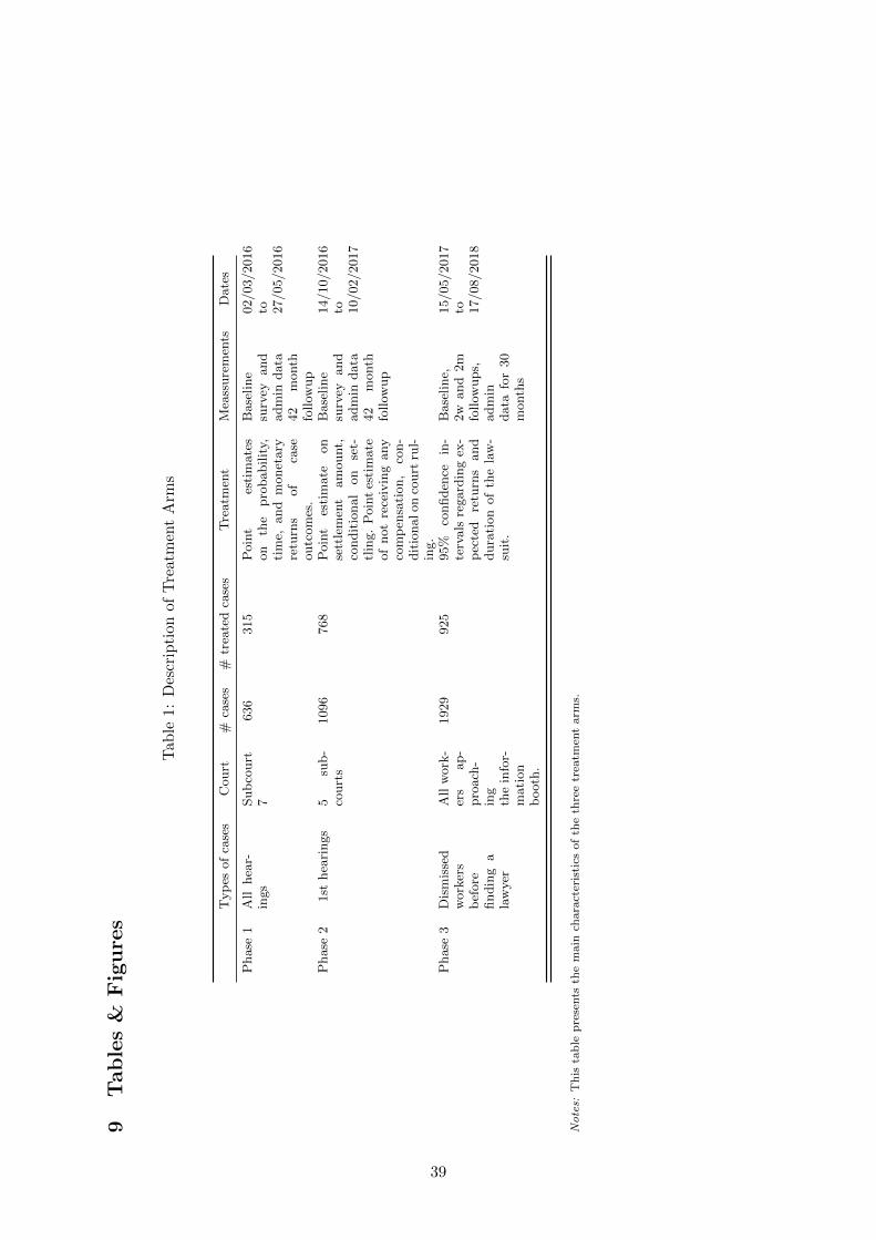
9T

ab

les

&F

igu

res

Tab

le1:

Des

crip

tion

ofT

reat

men

tA

rms

Typ

esof

case

sC

ourt

#ca

ses

#tr

eate

dca

ses

Tre

atm

ent

Mea

ssure

men

tsD

ate

s

Phase

1A

llhea

r-in

gs

Sub

court

7636

315

Poin

tes

tim

ate

son

the

pro

babilit

y,ti

me,

and

monet

ary

retu

rns

of

case

outc

om

es.

Base

line

surv

eyand

adm

indata

42

month

follow

up

02/03/2016

to 27/05/2016

Phase

21st

hea

rings

5su

b-

court

s1096

768

Poin

tes

tim

ate

on

sett

lem

ent

am

ount,

condit

ional

on

set-

tlin

g.

Poin

tes

tim

ate

of

not

rece

ivin

gany

com

pen

sati

on,

con-

dit

ionalon

court

rul-

ing.

Base

line

surv

eyand

adm

indata

42

month

follow

up

14/10/2016

to 10/02/2017

Phase

3D

ism

isse

dw

ork

ers

bef

ore

findin

ga

law

yer

All

work

-er

sap-

pro

ach

-in

gth

ein

for-

mati

on

booth

.

1929

925

95%

confiden

cein

-te

rvals

regard

ing

ex-

pec

ted

retu

rns

and

dura

tion

of

the

law

-su

it.

Base

line,

2w

and

2m

follow

ups,

adm

indata

for

30

month

s

15/05/2017

to 17/08/2018

No

tes:

Th

ista

ble

pre

sents

the

main

chara

cter

isti

csof

the

thre

etr

eatm

ent

arm

s.

39

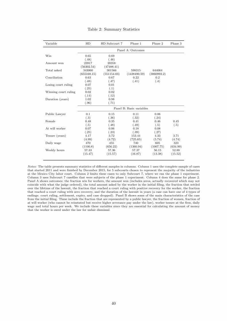
Table 2: Summary Statistics

Variable HD HD Subcourt 7 Phase 1 Phase 2 Phase 3

Panel A: Outcomes

Win 0.65 0.69(.48) (.46)

Amount won 23917 20358(56302.54) (47488.41)

Total asked 343060 301566 598315 644064(655168.15) (551154.03) (1438490.59) (3860993.2)

Conciliation 0.63 0.67 0.22 0.2(.48) (.47) (.41) (.4)

Losing court ruling 0.07 0.01(.25) (.1)

Winning court ruling 0.02 0.02(.14) (.12)

Duration (years) 1.02 0.98(.96) (.71)

Panel B: Basic variables

Public Lawyer 0.1 0.15 0.11 0.06(.3) (.36) (.32) (.24)

Female 0.48 0.35 0.41 0.46 0.45(.5) (.48) (.49) (.5) (.5)

At will worker 0.07 0.06 0.18 0.08(.25) (.23) (.39) (.27)

Tenure (years) 4.17 3.72 153.44 4.33 3.71(4.99) (4.72) (725.65) (5.74) (4.74)

Daily wage 470 455 740 605 323(1100.8) (656.22) (1360.94) (1007.75) (634.99)

Weekly hours 57.33 57.36 57.37 56.15 52.88(15.47) (15.57) (16.87) (13.38) (15.52)

Notes: The table presents summary statistics of different samples in columns. Column 1 uses the complete sample of casesthat started 2011 and were finished by December 2015, for 5 subcourts chosen to represent the majority of the industriesat the Mexico City labor court. Column 2 limits these cases to only Subcourt 7, where we ran the phase 1 experiment.Column 3 uses Subcourt 7 casefiles that were subjects of the phase 1 experiment. Column 4 does the same for phase 2.Panel A shows outcomes: the fraction win for workers, the amount won (includes zeros, actually recovered which may notcoincide with what the judge ordered), the total amount asked by the worker in the initial filing, the fraction that settledover the lifetime of the lawsuit, the fraction that reached a court ruling with positive recovery for the worker, the fractionthat reached a court ruling with zero recovery, and the duration of the lawsuit in years (a case can have one of 4 types ofendings: court ruling, settlement, expiry, and case dropped). Panel B shows some of the main characteristics of the casefrom the initial filing. These include the fraction that are represented by a public lawyer, the fraction of women, fraction ofat will worker (who cannot be reinstated but receive higher severance pay under the law), worker tenure at the firm, dailywage and total hours per week. We include these variables since they are essential for calculating the amount of moneythat the worker is owed under the law for unfair dismissal.

40

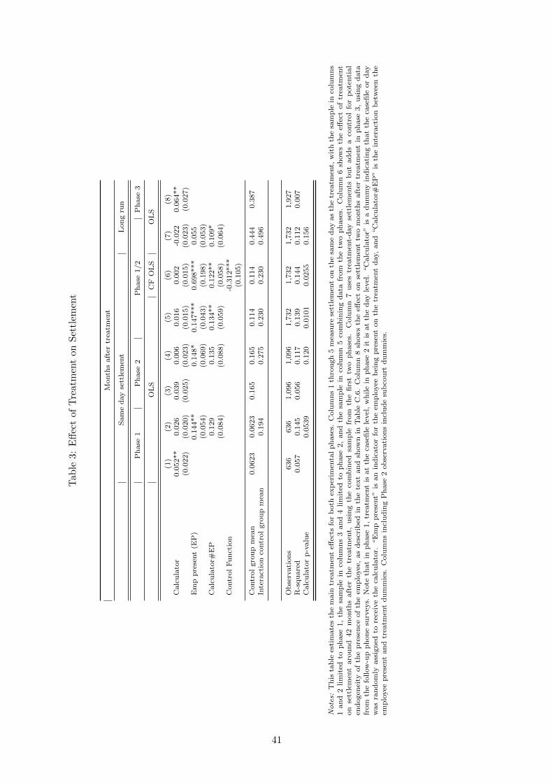
Tab

le3:

Eff

ect

ofT

reat

men

ton

Set

tlem

ent

Month

saft

ertr

eatm

ent

Sam

ed

ay

sett

lem

ent

Lon

gru

n

Ph

ase

1P

hase

2P

hase

1/2

Ph

ase

3

OL

SC

FO

LS

OL

S

(1)

(2)

(3)

(4)

(5)

(6)

(7)

(8)

Calc

ula

tor

0.0

52**

0.0

26

0.0

39

0.0

06

0.0

16

0.0

02

-0.0

22

0.0

64**

(0.0

22)

(0.0

20)

(0.0

25)

(0.0

23)

(0.0

15)

(0.0

15)

(0.0

23)

(0.0

27)

Em

pp

rese

nt

(EP

)0.1

44**

0.1

48*

0.1

47***

0.6

98***

0.0

55

(0.0

54)

(0.0

69)

(0.0

43)

(0.1

98)

(0.0

53)

Calc

ula

tor#

EP

0.1

29

0.1

35

0.1

34**

0.1

22**

0.1

09*

(0.0

84)

(0.0

88)

(0.0

59)

(0.0

58)

(0.0

64)

Contr

ol

Fu

nct

ion

-0.3

12***

(0.1

05)

Contr

ol

gro

up

mea

n0.0

623

0.0

623

0.1

65

0.1

65

0.1

14

0.1

14

0.4

44

0.3

87

Inte

ract

ion

contr

ol

gro

up

mea

n0.1

94

0.2

75

0.2

30

0.2

30

0.4

96

Ob

serv

ati

on

s636

636

1,0

96

1,0

96

1,7

32

1,7

32

1,7

32

1,9

27

R-s

qu

are

d0.0

57

0.1

45

0.0

56

0.1

17

0.1

39

0.1

44

0.1

12

0.0

07

Calc

ula

tor

p-v

alu

e0.0

539

0.1

20

0.0

101

0.0

255

0.1

56

No

tes:

Th

ista

ble

esti

mate

sth

em

ain

trea

tmen

teff

ects

for

both

exp

erim

enta

lp

hase

s.C

olu

mn

s1

thro

ugh

5m

easu

rese

ttle

men

ton

the

sam

ed

ay

as

the

trea

tmen

t,w

ith

the

sam

ple

inco

lum

ns

1an

d2

lim

ited

top

hase

1,

the

sam

ple

inco

lum

ns

3an

d4

lim

ited

top

hase

2,

an

dth

esa

mp

lein

colu

mn

5co

mb

inin

gd

ata

from

the

two

ph

ase

s.C

olu

mn

6sh

ow

sth

eeff

ect

of

trea

tmen

ton

sett

lem

ent

aro

un

d42

month

saft

erth

etr

eatm

ent,

usi

ng

the

com

bin

edsa

mp

lefr

om

the

firs

ttw

op

hase

s.C

olu

mn

7u

ses

trea

tmen

t-d

ay

sett

lem

ents

bu

tad

ds

aco

ntr

ol

for

pote

nti

al

end

ogen

eity

of

the

pre

sen

ceof

the

emp

loyee

,as

des

crib

edin

the

text

an

dsh

ow

nin

Table

C.6

.C

olu

mn

8sh

ow

sth

eeff

ect

on

sett

lem

ent

two

month

saft

ertr

eatm

ent

inph

ase

3,

usi

ng

data

from

the

follow

-up

ph

on

esu

rvey

s.N

ote

that

inp

hase

1,

trea

tmen

tis

at

the

case

file

level

,w

hile

inp

hase

2it

isat

the

day

level

.“C

alc

ula

tor”

isa

du

mm

yin

dic

ati

ng

that

the

case

file

or

day

was

ran

dom

lyass

ign

edto

rece

ive

the

calc

ula

tor.

“E

mp

pre

sent”

isan

ind

icato

rfo

rth

eem

plo

yee

bei

ng

pre

sent

on

the

trea

tmen

td

ay,

an

d“C

alc

ula

tor#

EP

”is

the

inte

ract

ion

bet

wee

nth

eem

plo

yee

pre

sent

an

dtr

eatm

ent

du

mm

ies.

Colu

mn

sin

clu

din

gP

hase

2ob

serv

ati

on

sin

clu

de

sub

cou

rtd

um

mie

s.

41

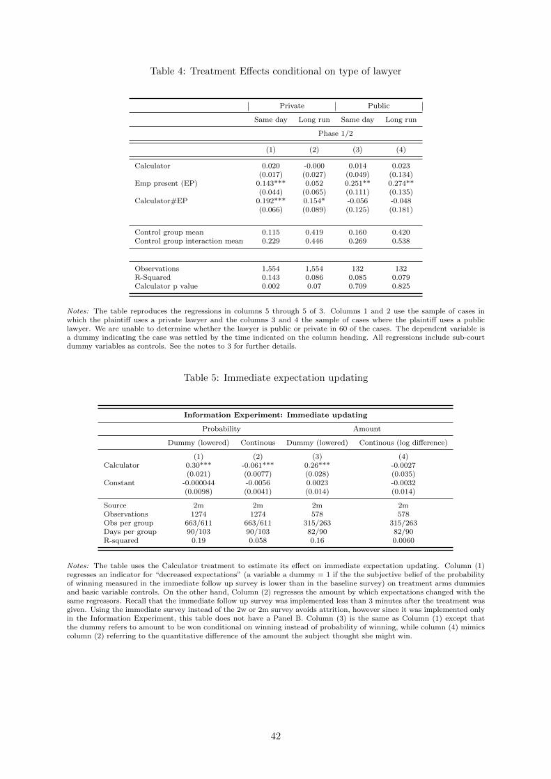
Table 4: Treatment Effects conditional on type of lawyer

Private Public

Same day Long run Same day Long run

Phase 1/2

(1) (2) (3) (4)

Calculator 0.020 -0.000 0.014 0.023(0.017) (0.027) (0.049) (0.134)

Emp present (EP) 0.143*** 0.052 0.251** 0.274**(0.044) (0.065) (0.111) (0.135)

Calculator#EP 0.192*** 0.154* -0.056 -0.048(0.066) (0.089) (0.125) (0.181)

Control group mean 0.115 0.419 0.160 0.420Control group interaction mean 0.229 0.446 0.269 0.538

Observations 1,554 1,554 132 132R-Squared 0.143 0.086 0.085 0.079Calculator p value 0.002 0.07 0.709 0.825

Notes: The table reproduces the regressions in columns 5 through 5 of 3. Columns 1 and 2 use the sample of cases inwhich the plaintiff uses a private lawyer and the columns 3 and 4 the sample of cases where the plaintiff uses a publiclawyer. We are unable to determine whether the lawyer is public or private in 60 of the cases. The dependent variable isa dummy indicating the case was settled by the time indicated on the column heading. All regressions include sub-courtdummy variables as controls. See the notes to 3 for further details.

Table 5: Immediate expectation updating

Information Experiment: Immediate updating

Probability Amount

Dummy (lowered) Continous Dummy (lowered) Continous (log difference)

(1) (2) (3) (4)Calculator 0.30*** -0.061*** 0.26*** -0.0027

(0.021) (0.0077) (0.028) (0.035)Constant -0.000044 -0.0056 0.0023 -0.0032

(0.0098) (0.0041) (0.014) (0.014)

Source 2m 2m 2m 2mObservations 1274 1274 578 578Obs per group 663/611 663/611 315/263 315/263Days per group 90/103 90/103 82/90 82/90R-squared 0.19 0.058 0.16 0.0060

Notes: The table uses the Calculator treatment to estimate its effect on immediate expectation updating. Column (1)regresses an indicator for “decreased expectations” (a variable a dummy = 1 if the the subjective belief of the probabilityof winning measured in the immediate follow up survey is lower than in the baseline survey) on treatment arms dummiesand basic variable controls. On the other hand, Column (2) regresses the amount by which expectations changed with thesame regressors. Recall that the immediate follow up survey was implemented less than 3 minutes after the treatment wasgiven. Using the immediate survey instead of the 2w or 2m survey avoids attrition, however since it was implemented onlyin the Information Experiment, this table does not have a Panel B. Column (3) is the same as Column (1) except thatthe dummy refers to amount to be won conditional on winning instead of probability of winning, while column (4) mimicscolumn (2) referring to the quantitative difference of the amount the subject thought she might win.

42

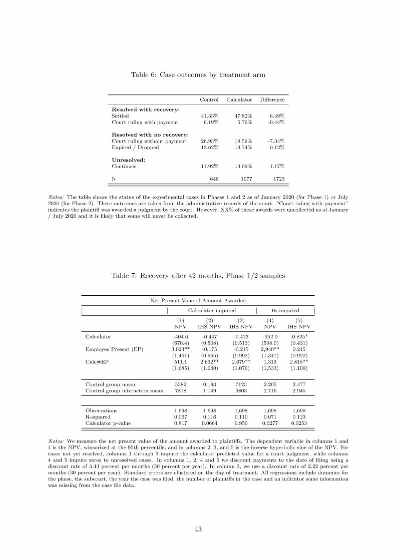
Table 6: Case outcomes by treatment arm

Control Calculator Difference

Resolved with recovery:Settled 41.33% 47.82% 6.49%Court ruling with payment 6.19% 5.76% -0.44%

Resolved with no recovery:Court ruling without payment 26.93% 19.59% -7.34%Expired / Dropped 13.62% 13.74% 0.12%

Unresolved:Continues 11.92% 13.09% 1.17%

N 646 1077 1723

Notes: The table shows the status of the experimental cases in Phases 1 and 2 as of January 2020 (for Phase 1) or July2020 (for Phase 2). These outcomes are taken from the administrative records of the court. “Court ruling with payment”indicates the plaintiff was awarded a judgment by the court. However, XX% of those awards were uncollected as of January/ July 2020 and it is likely that some will never be collected.

Table 7: Recovery after 42 months, Phase 1/2 samples

Net Present Vaue of Amount Awarded

Calculator imputed 0s imputed

(1) (2) (3) (4) (5)NPV IHS NPV IHS NPV NPV IHS NPV

Calculator -404.6 -0.447 -0.423 -952.0 -0.825*(670.4) (0.508) (0.513) (598.0) (0.431)

Employee Present (EP) 3,023** -0.175 -0.215 2,940** 0.245(1,461) (0.965) (0.992) (1,347) (0.922)

Calc#EP 511.1 2.632** 2.679** 1,313 2.818**(1,685) (1.040) (1.070) (1,533) (1.109)

Control group mean 5382 0.193 7123 2.205 2.477Control group interaction mean 7818 1.149 9803 2.716 2.945

Observations 1,698 1,698 1,698 1,698 1,698R-squared 0.067 0.116 0.110 0.071 0.123Calculator p-value 0.817 0.0664 0.950 0.0277 0.0253

Notes: We measure the net present value of the amount awarded to plaintiffs. The dependent variable in columns 1 and4 is the NPV, winsorized at the 95th percentile, and in columns 2, 3, and 5 is the inverse hyperbolic sine of the NPV. Forcases not yet resolved, columns 1 through 3 impute the calculator predicted value for a court judgment, while columns4 and 5 impute zeros to unresolved cases. In columns 1, 2, 4 and 5 we discount payments to the date of filing using adiscount rate of 3.43 percent per months (50 percent per year). In column 3, we use a discount rate of 2.22 percent permonths (30 percent per year). Standard errors are clustered on the day of treatment. All regressions include dummies forthe phase, the subcourt, the year the case was filed, the number of plaintiffs in the case and an indicator some informationwas missing from the case file data.

43

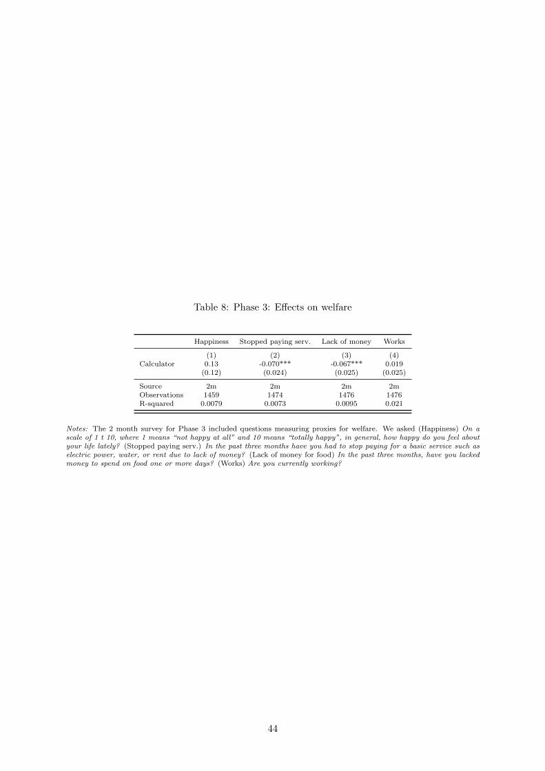
Table 8: Phase 3: Effects on welfare

Happiness Stopped paying serv. Lack of money Works

(1) (2) (3) (4)Calculator 0.13 -0.070*** -0.067*** 0.019

(0.12) (0.024) (0.025) (0.025)

Source 2m 2m 2m 2mObservations 1459 1474 1476 1476R-squared 0.0079 0.0073 0.0095 0.021

Notes: The 2 month survey for Phase 3 included questions measuring proxies for welfare. We asked (Happiness) On ascale of 1 t 10, where 1 means “not happy at all” and 10 means “totally happy”, in general, how happy do you feel aboutyour life lately? (Stopped paying serv.) In the past three months have you had to stop paying for a basic service such aselectric power, water, or rent due to lack of money? (Lack of money for food) In the past three months, have you lackedmoney to spend on food one or more days? (Works) Are you currently working?

44

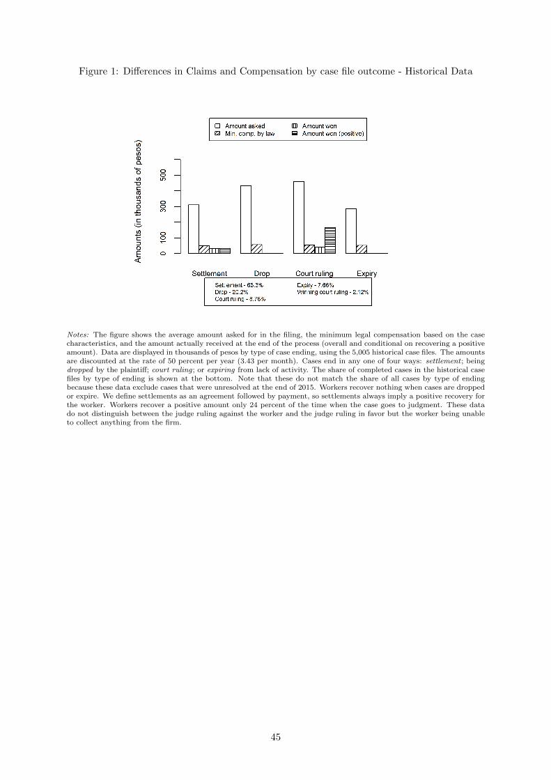
Figure 1: Differences in Claims and Compensation by case file outcome - Historical Data

Notes: The figure shows the average amount asked for in the filing, the minimum legal compensation based on the casecharacteristics, and the amount actually received at the end of the process (overall and conditional on recovering a positiveamount). Data are displayed in thousands of pesos by type of case ending, using the 5,005 historical case files. The amountsare discounted at the rate of 50 percent per year (3.43 per month). Cases end in any one of four ways: settlement ; beingdropped by the plaintiff; court ruling; or expiring from lack of activity. The share of completed cases in the historical casefiles by type of ending is shown at the bottom. Note that these do not match the share of all cases by type of endingbecause these data exclude cases that were unresolved at the end of 2015. Workers recover nothing when cases are droppedor expire. We define settlements as an agreement followed by payment, so settlements always imply a positive recovery forthe worker. Workers recover a positive amount only 24 percent of the time when the case goes to judgment. These datado not distinguish between the judge ruling against the worker and the judge ruling in favor but the worker being unableto collect anything from the firm.

45

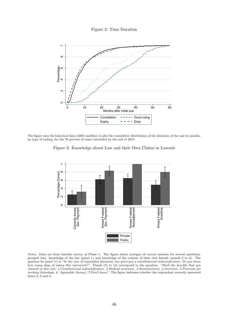
Figure 2: Time Duration

0.2

.4.6

.81

Perc

enta

ge

0 10 20 30 40 50 60Months after initial sue

Conciliation Court rulingExpiry Drop

The figure uses the historical data (5005 casefiles) to plot the cumulative distribution of the duration of the case in months,by type of ending, for the 70 percent of cases concluded by the end of 2015.

Figure 3: Knowledge about Law and their Own Claims in Lawsuit

0.2

.4.6

.81

Perc

enta

ge C

orre

ct

Cor

rect

ly k

now

sSe

v. P

aym

ent

Know

s if

aske

dSe

v. P

aym

ent

Know

s if

aske

dR

eins

tate

men

t

Know

s if

aske

dO

verti

me

PrivatePublic

Notes: Data are from baseline survey of Phase 1. The figure shows averages of correct answers for several questions,grouped into: knowledge of the law (panel 1) and knowledge of the content of their own lawsuit (panels 2 to 4). Thequestion for panel (1) is ”In the case of unjustified dismissal, law gives you a constitutional indemnification: Do you knowhow many days of salary this represents?”. Panels (2) to (4) correspond to the question: “Mark the benefits that youclaimed in this suit: 1.Constitutional indemnification, 2.Medical insurance, 3.Reinstatement, 4.Overtime, 5.Premium forworking Saturdays, 6. Aguinaldo (bonus), 7.Don’t know”. The figure indicates whether the respondent correctly answereditems 2, 3 and 4.

46

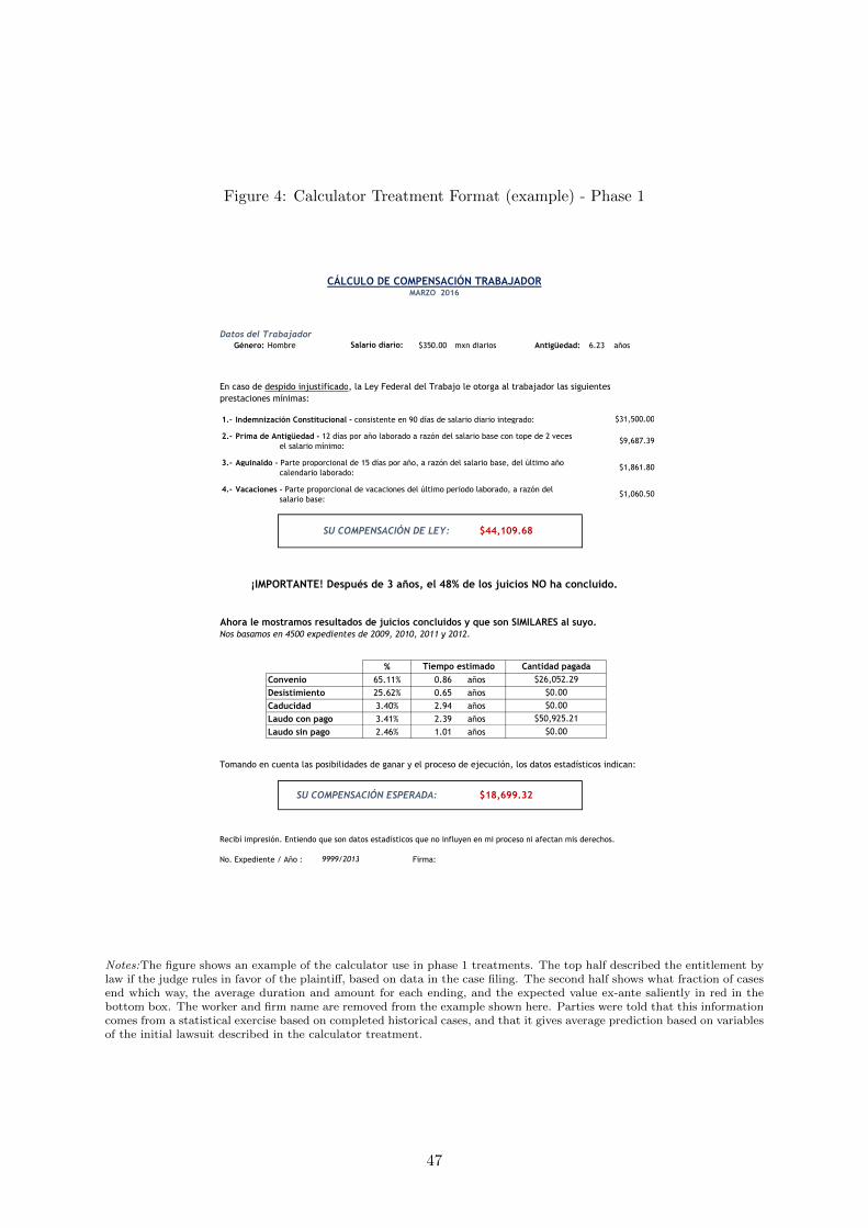
Figure 4: Calculator Treatment Format (example) - Phase 1

Datos del TrabajadorGénero: Hombre $350.00 mxn diarios Antigüedad: 6.23 años

En caso de despido injustificado, la Ley Federal del Trabajo le otorga al trabajador las siguientesprestaciones mínimas:1.- Indemnización Constitucional - consistente en 90 días de salario diario integrado:2.- Prima de Antigüedad - 12 días por año laborado a razón del salario base con tope de 2 veces

el salario mínimo:3.- Aguinaldo - Parte proporcional de 15 días por año, a razón del salario base, del último año

calendario laborado:4.- Vacaciones - Parte proporcional de vacaciones del último periodo laborado, a razón del

salario base:

Ahora le mostramos resultados de juicios concluidos y que son SIMILARES al suyo. Nos basamos en 4500 expedientes de 2009, 2010, 2011 y 2012.

%Convenio 65.11% 0.86 añosDesistimiento 25.62% 0.65 añosCaducidad 3.40% 2.94 añosLaudo con pago 3.41% 2.39 añosLaudo sin pago 2.46% 1.01 años

Tomando en cuenta las posibilidades de ganar y el proceso de ejecución, los datos estadísticos indican:

Recibí impresión. Entiendo que son datos estadísticos que no influyen en mi proceso ni afectan mis derechos.No. Expediente / Año : Firma:

$31,500.00$9,687.39

$1,861.80

$1,060.50

9999/2013

¡IMPORTANTE! Después de 3 años, el 48% de los juicios NO ha concluido.

SU COMPENSACIÓN DE LEY:

SU COMPENSACIÓN ESPERADA:

CÁLCULO DE COMPENSACIÓN TRABAJADORMARZO 2016

Tiempo estimado

$44,109.68

$18,699.32

Cantidad pagada$26,052.29

$0.00$0.00

$50,925.21$0.00

Salario diario:

Notes:The figure shows an example of the calculator use in phase 1 treatments. The top half described the entitlement bylaw if the judge rules in favor of the plaintiff, based on data in the case filing. The second half shows what fraction of casesend which way, the average duration and amount for each ending, and the expected value ex-ante saliently in red in thebottom box. The worker and firm name are removed from the example shown here. Parties were told that this informationcomes from a statistical exercise based on completed historical cases, and that it gives average prediction based on variablesof the initial lawsuit described in the calculator treatment.

47

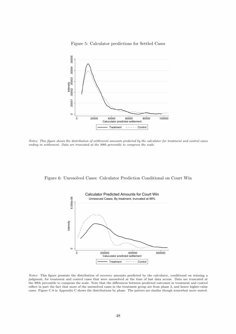
Figure 5: Calculator predictions for Settled Cases

0.0

0001

.000

02.0

0003

.000

04.0

0005

kden

sity

0 20000 40000 60000 80000 100000Caluculator predicted settlement

Treatment Control

Notes: This figure shows the distribution of settlement amounts predicted by the calculator for treatment and control casesending in settlement. Data are truncated at the 99th percentile to compress the scale.

Figure 6: Unresolved Cases: Calculator Prediction Conditional on Court Win

06.

000e

-06

kden

sity

0 200000 400000 600000Caluculator predicted settlement

Treatment Control

Unresoved Cases, By treatment, truncated at 99%Calculator Predicted Amounts for Court Win

Notes: This figure presents the distribution of recovery amounts predicted by the calculator, conditional on winning ajudgment, for treatment and control cases that were unresolved at the time of last data access. Data are truncated atthe 99th percentile to compress the scale. Note that the differences between predicted outcomes in treatment and controlreflect in part the fact that more of the unresolved cases in the treatment group are from phase 2, and hence higher-valuecases. Figure C.8 in Appendix C shows the distributions by phase. The patters are similar though somewhat more muted.

48

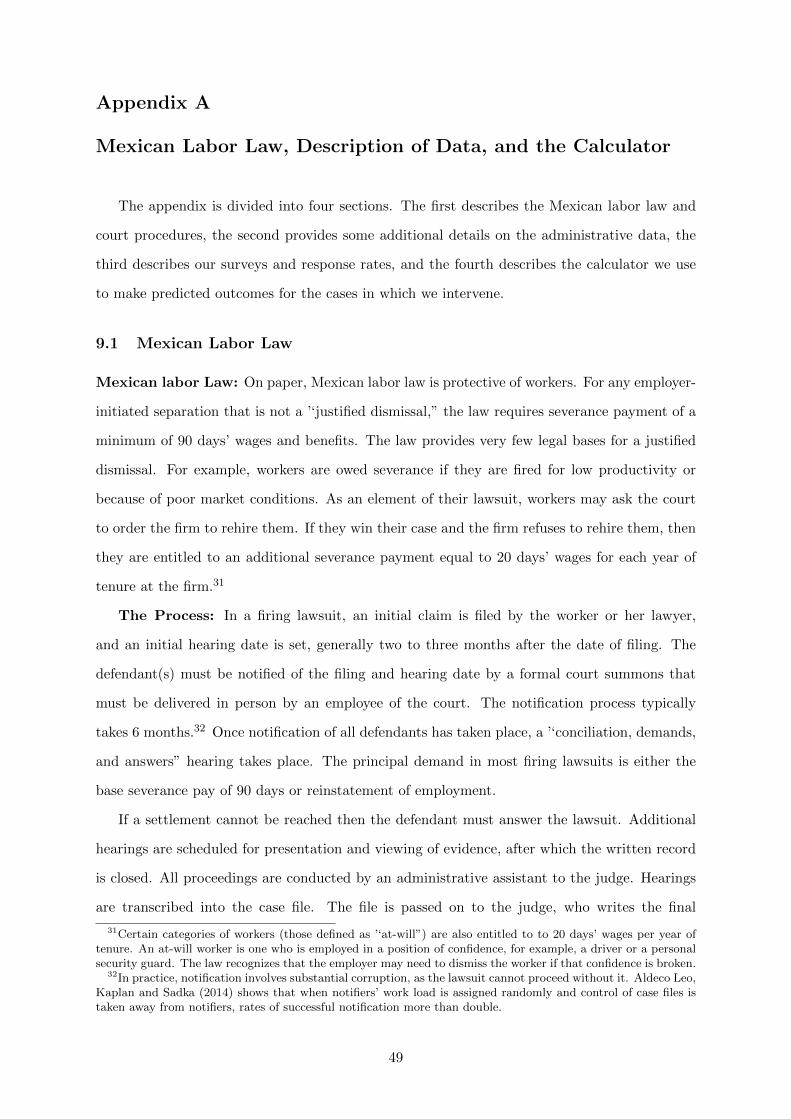
Appendix A

Mexican Labor Law, Description of Data, and the Calculator

The appendix is divided into four sections. The first describes the Mexican labor law and

court procedures, the second provides some additional details on the administrative data, the

third describes our surveys and response rates, and the fourth describes the calculator we use

to make predicted outcomes for the cases in which we intervene.

9.1 Mexican Labor Law

Mexican labor Law: On paper, Mexican labor law is protective of workers. For any employer-

initiated separation that is not a ’‘justified dismissal,” the law requires severance payment of a

minimum of 90 days’ wages and benefits. The law provides very few legal bases for a justified

dismissal. For example, workers are owed severance if they are fired for low productivity or

because of poor market conditions. As an element of their lawsuit, workers may ask the court

to order the firm to rehire them. If they win their case and the firm refuses to rehire them, then

they are entitled to an additional severance payment equal to 20 days’ wages for each year of

tenure at the firm.31

The Process: In a firing lawsuit, an initial claim is filed by the worker or her lawyer,

and an initial hearing date is set, generally two to three months after the date of filing. The

defendant(s) must be notified of the filing and hearing date by a formal court summons that

must be delivered in person by an employee of the court. The notification process typically

takes 6 months.32 Once notification of all defendants has taken place, a ’‘conciliation, demands,

and answers” hearing takes place. The principal demand in most firing lawsuits is either the

base severance pay of 90 days or reinstatement of employment.

If a settlement cannot be reached then the defendant must answer the lawsuit. Additional

hearings are scheduled for presentation and viewing of evidence, after which the written record

is closed. All proceedings are conducted by an administrative assistant to the judge. Hearings

are transcribed into the case file. The file is passed on to the judge, who writes the final

31Certain categories of workers (those defined as ’‘at-will”) are also entitled to to 20 days’ wages per year oftenure. An at-will worker is one who is employed in a position of confidence, for example, a driver or a personalsecurity guard. The law recognizes that the employer may need to dismiss the worker if that confidence is broken.

32In practice, notification involves substantial corruption, as the lawsuit cannot proceed without it. Aldeco Leo,Kaplan and Sadka (2014) shows that when notifiers’ work load is assigned randomly and control of case files istaken away from notifiers, rates of successful notification more than double.

49

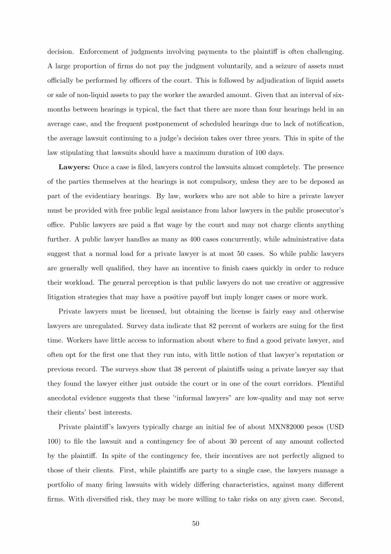
decision. Enforcement of judgments involving payments to the plaintiff is often challenging.

A large proportion of firms do not pay the judgment voluntarily, and a seizure of assets must

officially be performed by officers of the court. This is followed by adjudication of liquid assets

or sale of non-liquid assets to pay the worker the awarded amount. Given that an interval of six-

months between hearings is typical, the fact that there are more than four hearings held in an

average case, and the frequent postponement of scheduled hearings due to lack of notification,

the average lawsuit continuing to a judge’s decision takes over three years. This in spite of the

law stipulating that lawsuits should have a maximum duration of 100 days.

Lawyers: Once a case is filed, lawyers control the lawsuits almost completely. The presence

of the parties themselves at the hearings is not compulsory, unless they are to be deposed as

part of the evidentiary hearings. By law, workers who are not able to hire a private lawyer

must be provided with free public legal assistance from labor lawyers in the public prosecutor’s

office. Public lawyers are paid a flat wage by the court and may not charge clients anything

further. A public lawyer handles as many as 400 cases concurrently, while administrative data

suggest that a normal load for a private lawyer is at most 50 cases. So while public lawyers

are generally well qualified, they have an incentive to finish cases quickly in order to reduce

their workload. The general perception is that public lawyers do not use creative or aggressive

litigation strategies that may have a positive payoff but imply longer cases or more work.

Private lawyers must be licensed, but obtaining the license is fairly easy and otherwise

lawyers are unregulated. Survey data indicate that 82 percent of workers are suing for the first

time. Workers have little access to information about where to find a good private lawyer, and

often opt for the first one that they run into, with little notion of that lawyer’s reputation or

previous record. The surveys show that 38 percent of plaintiffs using a private lawyer say that

they found the lawyer either just outside the court or in one of the court corridors. Plentiful

anecdotal evidence suggests that these ’‘informal lawyers” are low-quality and may not serve

their clients’ best interests.

Private plaintiff’s lawyers typically charge an initial fee of about MXN$2000 pesos (USD

100) to file the lawsuit and a contingency fee of about 30 percent of any amount collected

by the plaintiff. In spite of the contingency fee, their incentives are not perfectly aligned to

those of their clients. First, while plaintiffs are party to a single case, the lawyers manage a

portfolio of many firing lawsuits with widely differing characteristics, against many different

firms. With diversified risk, they may be more willing to take risks on any given case. Second,

50

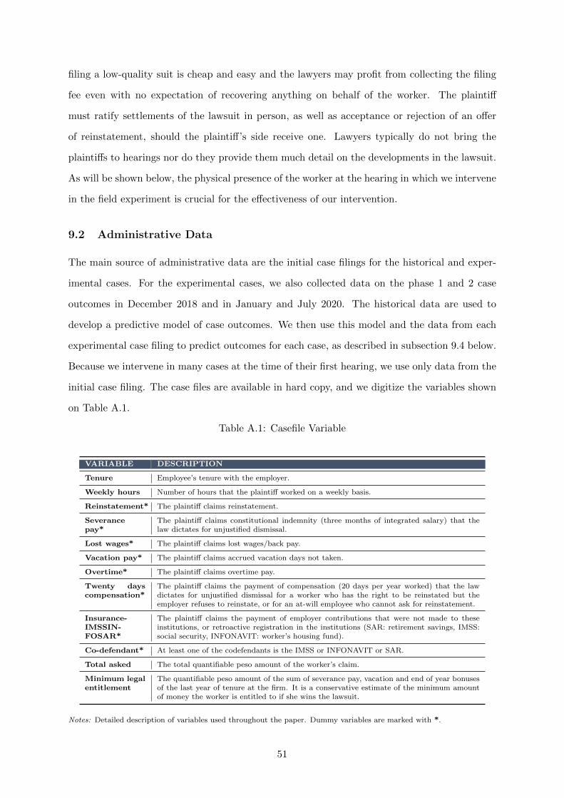
filing a low-quality suit is cheap and easy and the lawyers may profit from collecting the filing

fee even with no expectation of recovering anything on behalf of the worker. The plaintiff

must ratify settlements of the lawsuit in person, as well as acceptance or rejection of an offer

of reinstatement, should the plaintiff’s side receive one. Lawyers typically do not bring the

plaintiffs to hearings nor do they provide them much detail on the developments in the lawsuit.

As will be shown below, the physical presence of the worker at the hearing in which we intervene

in the field experiment is crucial for the effectiveness of our intervention.

9.2 Administrative Data

The main source of administrative data are the initial case filings for the historical and exper-

imental cases. For the experimental cases, we also collected data on the phase 1 and 2 case

outcomes in December 2018 and in January and July 2020. The historical data are used to

develop a predictive model of case outcomes. We then use this model and the data from each

experimental case filing to predict outcomes for each case, as described in subsection 9.4 below.

Because we intervene in many cases at the time of their first hearing, we use only data from the

initial case filing. The case files are available in hard copy, and we digitize the variables shown

on Table A.1.

Table A.1: Casefile Variable

VARIABLE DESCRIPTION

Tenure Employee’s tenure with the employer.

Weekly hours Number of hours that the plaintiff worked on a weekly basis.

Reinstatement* The plaintiff claims reinstatement.

Severancepay*

The plaintiff claims constitutional indemnity (three months of integrated salary) that thelaw dictates for unjustified dismissal.

Lost wages* The plaintiff claims lost wages/back pay.

Vacation pay* The plaintiff claims accrued vacation days not taken.

Overtime* The plaintiff claims overtime pay.

Twenty dayscompensation*

The plaintiff claims the payment of compensation (20 days per year worked) that the lawdictates for unjustified dismissal for a worker who has the right to be reinstated but theemployer refuses to reinstate, or for an at-will employee who cannot ask for reinstatement.

Insurance-IMSSIN-FOSAR*

The plaintiff claims the payment of employer contributions that were not made to theseinstitutions, or retroactive registration in the institutions (SAR: retirement savings, IMSS:social security, INFONAVIT: worker’s housing fund).

Co-defendant* At least one of the codefendants is the IMSS or INFONAVIT or SAR.

Total asked The total quantifiable peso amount of the worker’s claim.

Minimum legalentitlement

The quantifiable peso amount of the sum of severance pay, vacation and end of year bonusesof the last year of tenure at the firm. It is a conservative estimate of the minimum amountof money the worker is entitled to if she wins the lawsuit.

Notes: Detailed description of variables used throughout the paper. Dummy variables are marked with *.

51

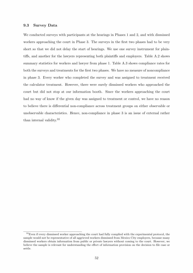
9.3 Survey Data

We conducted surveys with participants at the hearings in Phases 1 and 2, and with dismissed

workers approaching the court in Phase 3. The surveys in the first two phases had to be very

short so that we did not delay the start of hearings. We use one survey instrument for plain-

tiffs, and another for the lawyers representing both plaintiffs and employers. Table A.2 shows

summary statistics for workers and lawyer from phase 1. Table A.3 shows compliance rates for

both the surveys and treatments for the first two phases. We have no measure of noncompliance

in phase 3. Every worker who completed the survey and was assigned to treatment received

the calculator treatment. However, there were surely dismissed workers who approached the

court but did not stop at our information booth. Since the workers approaching the court

had no way of know if the given day was assigned to treatment or control, we have no reason

to believe there is differential non-compliance across treatment groups on either observable or

unobservable characteristics. Hence, non-compliance in phase 3 is an issue of external rather

than internal validity.33

33Even if every dismissed worker approaching the court had fully complied with the experimental protocol, thesample would not be representative of all aggrieved workers dismissed from Mexico City employers, because manydismissed workers obtain information from public or private lawyers without coming to the court. However, webelieve the sample is relevant for understanding the effect of information provision on the decision to file case orsettle.

52

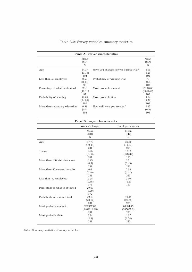
Table A.2: Survey variables summary statistics

Panel A: worker characteristics

Mean Mean(SD) (SD)

N N

Age 44.37 Have you changed lawyer during trial? 0.09(13.18) (0.29)

102 102Less than 50 employees 0.59 Probability of winning trial 79

(0.49) (21.3)96 102

Percentage of what is obtained 28.3 Most probable amount 97116.66(11.11) (355749)

57 102Probability of winning 48.68 Most probable time 3.64

(34.06) (9.76)102 102

More than secondary education 0.58 How well were you treated? 0.45(0.5) (0.5)102 102

Panel B: lawyer characteristics

Worker’s lawyer Employer’s lawyer

Mean Mean(SD) (SD)

N N

Age 37.79 36.56(12.43) (10.97)

231 223Tenure 9.25 18.65

(8.88) (143.32)181 193

More than 100 historical cases 0.49 0.61(0.5) (0.49)231 223

More than 30 current lawsuits 0.6 0.68(0.49) (0.47)231 223

Less than 50 employees 0.65 0.46(0.48) (0.5)173 151

Percentage of what is obtained 29.69(7.79)172

Probability of winning trial 72.19 70.48(20.14) (21.53)

231 223Most probable amount 237957.65 66884.79

(1482119.93) (285657.2)231 223

Most probable time 3.94 4.17(2.3) (2.54)231 223

Notes: Summary statistics of survey variables.

53

Tab

leA

.3:

Com

pli

ance

Rat

e

(a)

Ph

ase

1

Gro

up

NC

om

plian

cew

ith

trea

tmen

tC

om

plian

cew

ith

base

lin

esu

rvey

Com

plian

cew

ith

exit

surv

ey

Pla

inti

ffD

efen

dant

Both

Any

Pla

inti

ffD

efen

dant

Both

Any

Pla

inti

ffD

efen

dant

Both

Any

Contr

ol

321

--

--

50.7

835.5

18.7

277.5

739.8

824.3

94.3

958.5

7C

alc

ula

tor

315

77.6

573.0

375.8

179.7

248.2

533.6

512.3

869.5

238.6

325.8

688.4

754.8

3

(b)

Ph

ase

2

Gro

up

NC

om

plian

cew

ith

trea

tmen

tC

om

plian

cew

ith

surv

ey

Pla

inti

ffD

efen

dant

Both

Any

Pla

inti

ffD

efen

dant

Both

Any

Contr

ol

329

--

--

--

-C

alc

ula

tor

762

72.7

63.7

849.0

887.4

54.3

348.2

949.0

887.4

(c)

%S

how

su

p

Ph

ase

1P

hase

2

Contr

ol

Calc

ula

tor

Contr

ol

Calc

ula

tor

Em

plo

yee

0.1

93

0.1

97

0.1

22

0.1

65

Em

pL

aw

yer

0.8

47

0.8

32

0.8

50.8

53

Fir

mL

aw

yer

0.7

38

0.7

62

0.4

34

0.4

44

No

tes:

Com

plian

cera

tefo

rea

chp

hase

,b

oth

for

trea

tmen

tan

dsu

rvey

.E

ach

pan

elsh

ow

sth

ep

erce

nta

ge

com

plian

cew

ith

trea

tmen

tan

dsu

rvey

for

pla

inti

ff’

sid

e,d

efen

dant’

ssi

de,

both

,an

dany.

Inp

hase

1,

we

did

not

mea

sure

com

plian

cew

ith

trea

tmen

tat

the

part

yle

vel

bu

tra

ther

at

the

case

file

level

,so

that

for

exam

ple

the

74.1

6u

nd

erth

eco

lum

n”b

oth

”fo

rco

mp

lian

cew

ith

trea

tmen

tm

ean

sth

at

am

on

gth

eca

sefi

les

for

wh

ich

both

part

ies

show

edu

pto

the

hea

rin

g,

we

wer

eab

leto

giv

eth

eca

lcu

lato

rto

at

least

on

eof

the

part

ies

in74.1

6p

erce

nt

of

the

case

s.A

lso,

inp

hase

1w

eh

ad

an

exit

surv

eyin

ad

dit

ion

toth

eb

ase

lin

esu

rvey

.In

ph

ase

2,

we

did

mea

sure

com

plian

cew

ith

the

trea

tmen

tby

part

y.O

nth

eoth

erh

an

d,

note

from

pan

el(b

)th

at

sin

cein

ph

ase

2co

ntr

ol

days

wer

ed

ays

that

no

imp

lem

enti

ng

per

son

nel

wer

ep

rese

nt

inth

esu

bco

urt

s,w

eh

ave

nei

ther

trea

tmen

tn

or

surv

eyco

mp

lian

cefo

rth

eco

ntr

ol

gro

up

.P

anel

(c)

show

sfr

om

the

cou

rt’s

ad

min

istr

ati

ve

data

wh

osh

ow

su

pto

the

hea

rin

gs

for

each

of

the

two

ph

ase

s,sp

lit

by

emp

loyee

,em

plo

yee

law

yer

,an

dfi

rmla

wyer

.

54

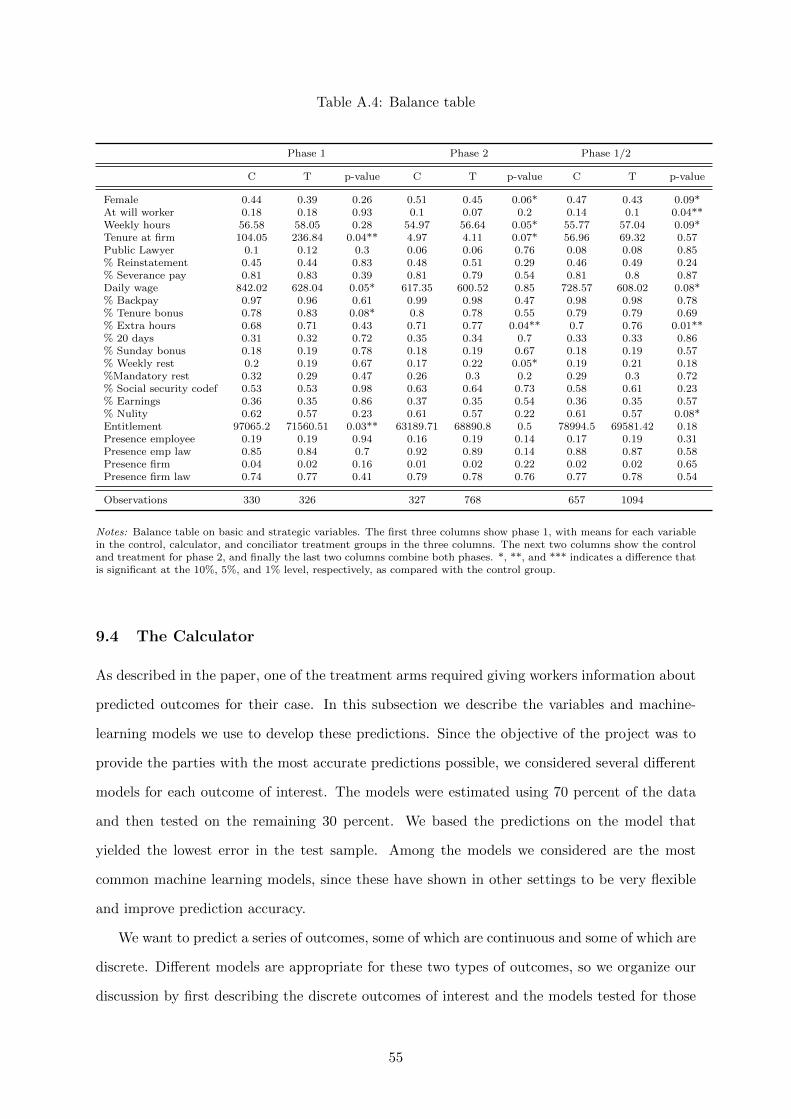
Table A.4: Balance table

Phase 1 Phase 2 Phase 1/2

C T p-value C T p-value C T p-value

Female 0.44 0.39 0.26 0.51 0.45 0.06* 0.47 0.43 0.09*At will worker 0.18 0.18 0.93 0.1 0.07 0.2 0.14 0.1 0.04**Weekly hours 56.58 58.05 0.28 54.97 56.64 0.05* 55.77 57.04 0.09*Tenure at firm 104.05 236.84 0.04** 4.97 4.11 0.07* 56.96 69.32 0.57Public Lawyer 0.1 0.12 0.3 0.06 0.06 0.76 0.08 0.08 0.85% Reinstatement 0.45 0.44 0.83 0.48 0.51 0.29 0.46 0.49 0.24% Severance pay 0.81 0.83 0.39 0.81 0.79 0.54 0.81 0.8 0.87Daily wage 842.02 628.04 0.05* 617.35 600.52 0.85 728.57 608.02 0.08*% Backpay 0.97 0.96 0.61 0.99 0.98 0.47 0.98 0.98 0.78% Tenure bonus 0.78 0.83 0.08* 0.8 0.78 0.55 0.79 0.79 0.69% Extra hours 0.68 0.71 0.43 0.71 0.77 0.04** 0.7 0.76 0.01**% 20 days 0.31 0.32 0.72 0.35 0.34 0.7 0.33 0.33 0.86% Sunday bonus 0.18 0.19 0.78 0.18 0.19 0.67 0.18 0.19 0.57% Weekly rest 0.2 0.19 0.67 0.17 0.22 0.05* 0.19 0.21 0.18%Mandatory rest 0.32 0.29 0.47 0.26 0.3 0.2 0.29 0.3 0.72% Social security codef 0.53 0.53 0.98 0.63 0.64 0.73 0.58 0.61 0.23% Earnings 0.36 0.35 0.86 0.37 0.35 0.54 0.36 0.35 0.57% Nulity 0.62 0.57 0.23 0.61 0.57 0.22 0.61 0.57 0.08*Entitlement 97065.2 71560.51 0.03** 63189.71 68890.8 0.5 78994.5 69581.42 0.18Presence employee 0.19 0.19 0.94 0.16 0.19 0.14 0.17 0.19 0.31Presence emp law 0.85 0.84 0.7 0.92 0.89 0.14 0.88 0.87 0.58Presence firm 0.04 0.02 0.16 0.01 0.02 0.22 0.02 0.02 0.65Presence firm law 0.74 0.77 0.41 0.79 0.78 0.76 0.77 0.78 0.54

Observations 330 326 327 768 657 1094

Notes: Balance table on basic and strategic variables. The first three columns show phase 1, with means for each variablein the control, calculator, and conciliator treatment groups in the three columns. The next two columns show the controland treatment for phase 2, and finally the last two columns combine both phases. *, **, and *** indicates a difference thatis significant at the 10%, 5%, and 1% level, respectively, as compared with the control group.

9.4 The Calculator

As described in the paper, one of the treatment arms required giving workers information about

predicted outcomes for their case. In this subsection we describe the variables and machine-

learning models we use to develop these predictions. Since the objective of the project was to

provide the parties with the most accurate predictions possible, we considered several different

models for each outcome of interest. The models were estimated using 70 percent of the data

and then tested on the remaining 30 percent. We based the predictions on the model that

yielded the lowest error in the test sample. Among the models we considered are the most

common machine learning models, since these have shown in other settings to be very flexible

and improve prediction accuracy.

We want to predict a series of outcomes, some of which are continuous and some of which are

discrete. Different models are appropriate for these two types of outcomes, so we organize our

discussion by first describing the discrete outcomes of interest and the models tested for those

55

outcomes, and then describe the continuous outcomes of interest and the models we tested for

those outcomes. We then describe the calculator templates used in both the first and second

phase of the project.

For the calculators used in both phases, and for both the continuous and discrete models,

we fed the models with the same set of input variables, all from the initial case filing. This

is because, for operational reasons we could not use procedures that occur after the filing of

the lawsuit, such as evidence submission. Also, the court wanted us to develop a parsimonious

calculator that could be used in pre-judicial conciliation meetings prior to the plaintiff filing

suit.

Discrete outcome models

The expected payment made to the plaintiff is a function of which party prevails and the amount

transferred conditional on the outcome. There are five ways a case can end:

1. Settlement: The case may end with a voluntary agreement between the parties where

the the plaintiff accepts a sum of money to cease the lawsuit and renounce the legal right

to sue again for the same reason. To be valid, these settlements must be registered at the

court, and therefore included in our administrative data.

2. Court ruling with positive compensation: Cases may proceed to a ruling by a judge

that decides which side is wins the lawsuit and how much should be paid to the plaintiff.

We classify an outcome as Court ruling with positive compensation if the case ends in a

ruling by the judge and the worker actually collects a positive amount.34

3. Court ruling with zero compensation: The judge may also rule in the defendant’s

favor. In that event the worker receives nothing. However, the worker may also receive

nothing if the judge rules in her favor, but she is unable to recover any of the judgment

amount from the defendant. Defendants use a variety of strategies to avoid paying judg-

ments, so the win but collect nothing outcome is not uncommon. The court records that

we digitized did not allow us to differentiate between these two outcomes. We do not

see this as an important shortcoming since from the point of view of the plaintiff what

matters is the amount she receives.

34Because court rulings with positive collection are uncommon (3.3 percent of cases) we face the the problemof unbalancedness of our court rulings sample. To deal with this problem we used a Synthetic Minority Over-Sampling Technique (see Chawla et.al., 2002) and did a 80-20 train vs. test split on our data.

56

4. Dropped: A case can be dropped by the plaintiff at any time during the legal proceedings.

The difference between dropped and settlement is that it can be done unilaterally by the

plaintiff and no payment to the defendant is registered. Our understanding is that when

cases are dropped it is because the plaintiff has little evidence to support the case. It is

a decision of the plaintiff and not a mandate by the court.

5. Expiry: Finally, a labor suit may expire if the court requires information to continue

the procedure, including items of evidence presented by one of the parties that the court

needs to view before concluding the hearings procedure if proofs are not provided in a

span of 4 months.

In our historical data of cases filed in 2011 and completed by the end of 2015, 63.3 percent

end in settlement, 2.0 percent in a court ruling with positive collection, 6.6 percent with a court

ruling with nothing collected, 20.3 percent expire and 7.6 percent are dropped.

We want to estimate the probability that a case with characteristics Xi ends in each of

the five ways described above. We have a choice of estimating a single multinomial model

or separate bivariate outcome models. We chose the bivariate option for simplicity. But to

ensure that the probabilities summed to one, we set the probability of expiry equal one minus

the sum of the probabilities of the other four outcomes.35 We therefore estimated models for

four bivariate outcomes, using each the following methods: (a) Logistic Regression, (b) Probit,

(c) Random Forest36, (d) Single-hidden-layer Neural Network (20 nodes in the hidden layer

and 10% weight decay), (e) Gradient Boosting.37 Models were estimated in a random sample

training set made of 70 percent of the observation. The remaining 30 percent was used as a

test set. For each model hyperparameters were chosen to minimize mean square error in the

test set (MSE-T) using cross-validation. Once hyperparameters for each model were chosen,

we chose among those optimized models bases on their mean square error. For each of the 5

discrete outcomes we want to predict we kept the model with the highest correlation between

Y and Y in the test set.38 Table A.5 shows the accuracy rate for each of these 5 outcomes and

for each of the 5 models, highlighting in grey the one chosen. The correlations range from 0.61

35We also estimated a multinomial model. The results were similar, which is why we chose the bivariate modelsfor simplicity.

36We performed grid search in order to find the best hyperparameter setting. We compared 7 different modelswith the number of trees ranging between 900 and 1500. Our final model resulted in a Random Forest of 1200CARTs, which yielded an 86 percent accuracy rate on test classification.

37This was implemented with off the shelf models in R : e1071, randomForest, neuralnet, caTools, mboost.38For the outcome of settlement, we find that the correlation between Y and Y is very slightly higher for

Random Forest than for Logit, but we use the Logit model because it was simpler to implement in the field.

57

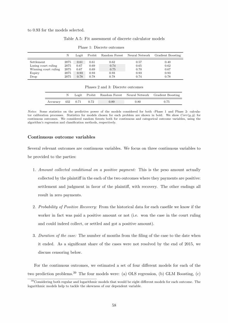
to 0.93 for the models selected.

Table A.5: Fit assessment of discrete calculator models

Phase 1: Discrete outcomes

N Logit Probit Random Forest Neural Network Gradient Boosting

Settlement 2075 0.61 0.61 0.62 0.57 0.40Losing court ruling 2075 0.67 0.69 0.74 0.65 0.62Winning court ruling 2075 0.67 0.69 0.75 0.70 0.67Expiry 2075 0.93 0.93 0.93 0.93 0.93Drop 2075 0.78 0.78 0.78 0.74 0.78

Phases 2 and 3: Discrete outcomes

N Logit Probit Random Forest Neural Network Gradient Boosting

Accuracy 432 0.71 0.72 0.89 0.80 0.75

Notes: Some statistics on the predictive power of the models considered for both -Phase 1 and Phase 2- calcula-tor calibration processes. Statistics for models chosen for each problem are shown in bold. We show Corr(y, y) forcontinuous outcomes. We considered random forests both for continuous and categorical outcome variables, using thealgorithm’s regression and classification methods, respectively.

Continuous outcome variables

Several relevant outcomes are continuous variables. We focus on three continuous variables to

be provided to the parties:

1. Amount collected conditional on a positive payment: This is the peso amount actually

collected by the plaintiff in the each of the two outcomes where they payments are positive:

settlement and judgment in favor of the plaintiff, with recovery. The other endings all

result in zero payments.

2. Probability of Positive Recovery: From the historical data for each casefile we know if the

worker in fact was paid a positive amount or not (i.e. won the case in the court ruling

and could indeed collect, or settled and got a positive amount).

3. Duration of the case: The number of months from the filing of the case to the date when

it ended. As a significant share of the cases were not resolved by the end of 2015, we

discuss censoring below.

For the continuous outcomes, we estimated a set of four different models for each of the

two prediction problems.39 The four models were: (a) OLS regression, (b) GLM Boosting, (c)

39Considering both regular and logarithmic models that would be eight different models for each outcome. Thelogarithmic models help to tackle the skewness of our dependent variable.

58

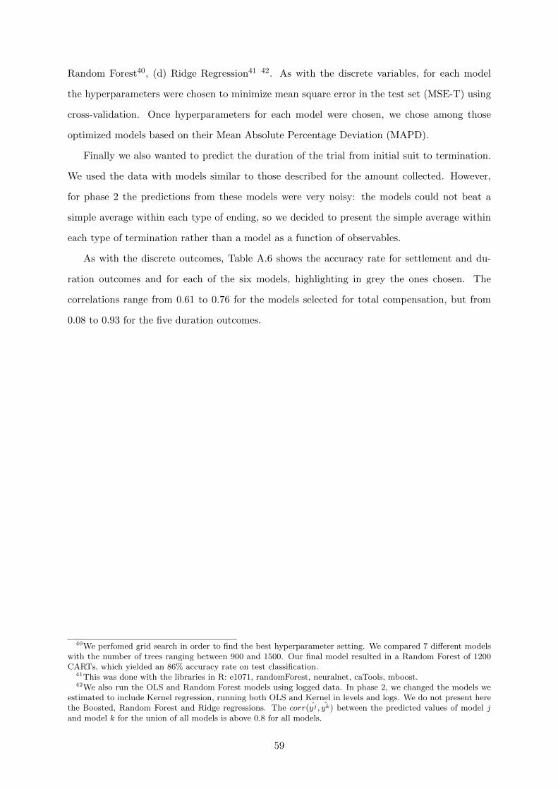
Random Forest40, (d) Ridge Regression41 42. As with the discrete variables, for each model

the hyperparameters were chosen to minimize mean square error in the test set (MSE-T) using

cross-validation. Once hyperparameters for each model were chosen, we chose among those

optimized models based on their Mean Absolute Percentage Deviation (MAPD).

Finally we also wanted to predict the duration of the trial from initial suit to termination.

We used the data with models similar to those described for the amount collected. However,

for phase 2 the predictions from these models were very noisy: the models could not beat a

simple average within each type of ending, so we decided to present the simple average within

each type of termination rather than a model as a function of observables.

As with the discrete outcomes, Table A.6 shows the accuracy rate for settlement and du-

ration outcomes and for each of the six models, highlighting in grey the ones chosen. The

correlations range from 0.61 to 0.76 for the models selected for total compensation, but from

0.08 to 0.93 for the five duration outcomes.

40We perfomed grid search in order to find the best hyperparameter setting. We compared 7 different modelswith the number of trees ranging between 900 and 1500. Our final model resulted in a Random Forest of 1200CARTs, which yielded an 86% accuracy rate on test classification.

41This was done with the libraries in R: e1071, randomForest, neuralnet, caTools, mboost.42We also run the OLS and Random Forest models using logged data. In phase 2, we changed the models we

estimated to include Kernel regression, running both OLS and Kernel in levels and logs. We do not present herethe Boosted, Random Forest and Ridge regressions. The corr(yj , yk) between the predicted values of model jand model k for the union of all models is above 0.8 for all models.

59

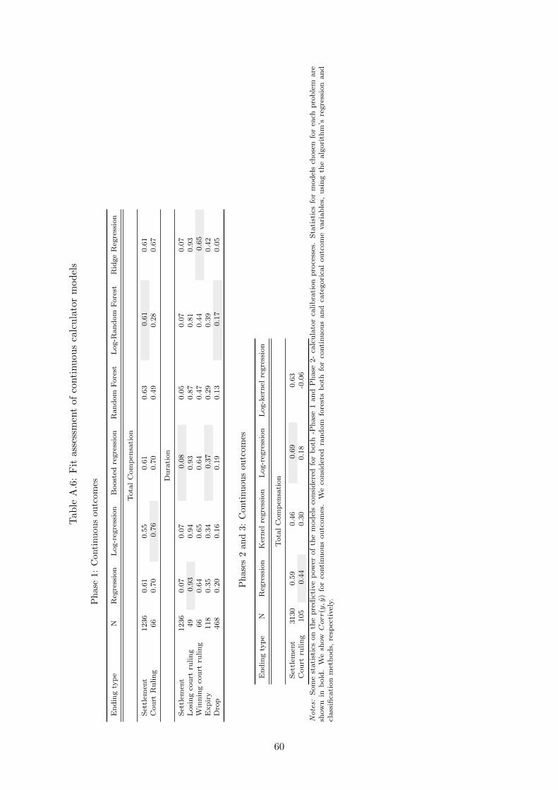
Tab

leA

.6:

Fit

asse

ssm

ent

ofco

nti

nu

ous

calc

ula

tor

model

s

Ph

ase

1:C

onti

nu

ous

outc

omes

En

din

gty

pe

NR

egre

ssio

nL

og-r

egre

ssio

nB

oost

edre

gre

ssio

nR

an

dom

Fore

stL

og-R

an

dom

Fore

stR

idge

Reg

ress

ion

Tota

lC

om

pen

sati

on

Set

tlem

ent

1236

0.6

10.5

50.6

10.6

30.6

10.6

1C

ou

rtR

ulin

g66

0.7

00.7

60.7

00.4

90.2

80.6

7

Du

rati

on

Set

tlem

ent

1236

0.0

70.0

70.0

80.0

50.0

70.0

7L

osi

ng

cou

rtru

lin

g49

0.9

30.9

40.9

30.8

70.8

10.9

3W

inn

ing

cou

rtru

lin

g66

0.6

40.6

50.6

40.4

70.4

40.6

5E

xp

iry

118

0.3

50.3

40.3

70.2

90.3

90.4

2D

rop

468

0.2

00.1

60.1

90.1

30.1

70.0

5

Ph

ases

2an

d3:

Con

tinu

ous

ou

tcom

es

En

din

gty

pe

NR

egre

ssio

nK

ern

elre

gre

ssio

nL

og-r

egre

ssio

nL

og-k

ern

elre

gre

ssio

n

Tota

lC

om

pen

sati

on

Set

tlem

ent

3130

0.5

90.4

60.6

90.6

3C

ou

rtru

lin

g105

0.4

40.3

00.1

8-0

.06

No

tes:

Som

est

ati

stic

son

the

pre

dic

tive

pow

erof

the

mod

els

con

sid

ered

for

both

-Ph

ase

1an

dP

hase

2-

calc

ula

tor

calib

rati

on

pro

cess

es.

Sta

tist

ics

for

mod

els

chose

nfo

rea

chp

rob

lem

are

show

nin

bold

.W

esh

owCorr(y,y

)fo

rco

nti

nu

ou

sou

tcom

es.

We

con

sid

ered

ran

dom

fore

sts

both

for

conti

nu

ou

san

dca

tegori

cal

ou

tcom

evari

ab

les,

usi

ng

the

alg

ori

thm

’sre

gre

ssio

nan

dcl

ass

ifica

tion

met

hod

s,re

spec

tivel

y.

60

Other issues: Censoring

All of the models are estimated on a sample of cases filed in 2011 and completed by the end

of 2015. The fact that the sample contains only the cases that were resolved could introduce

a bias in the prediction of outcomes of ongoing cases. For example, if we are interested in

the probability of winning eventually and if cases with larger expected payouts take longer

to resolve, then excluding the unresolved cases may produce an underestimate of the average

payments in all cases.

We are aware of this bias and it was communicated to the parties when the calculator

information was provided. Although we cannot know how large the bias is, we performed two

exercises that suggest it is not large. First, we compare characteristics of ongoing cases with

those of the historical cases used in the models. In Figure A.1 we show that the two sets of

cases are similar. The second exercise compares the characteristics of completed and continuing

lawsuits within the historical data. To do this we drew a random sample of 956 cases filed

in 2011 that were not finished by 2015 (i.e. this represents the complement of our historical

dataset). We compare these 956 cases to the completed cases used to develop the models.

Figure A.2 reports the results. There are no significant differences between these two samples,

and the magnitude of the measured differences are all very small.

61

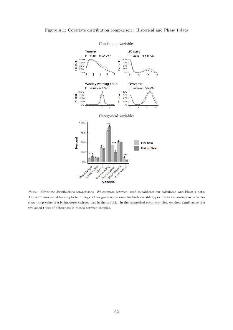
Figure A.1: Covariate distribution comparison : Historical and Phase 1 data

Continuous variables

Categorical variables

Notes: Covariate distributions comparisons. We compare between -used to calibrate our calculator- and Phase 1 data.

All continuous variables are plotted in logs. Color guide is the same for both variable types. Plots for continuous variables

show the p-value of a KolmogorovSmirnov test in the subtitle. In the categorical covariates plot, we show significance of a

two-sided t-test of differences in means between samples.

62

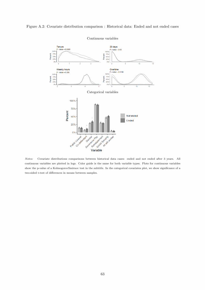
Figure A.2: Covariate distribution comparison : Historical data: Ended and not ended cases

Continuous variables

Categorical variables

Notes: Covariate distributions comparisons between historical data cases: ended and not ended after 3 years. All

continuous variables are plotted in logs. Color guide is the same for both variable types. Plots for continuous variables

show the p-value of a KolmogorovSmirnov test in the subtitle. In the categorical covariates plot, we show significance of a

two-sided t-test of differences in means between samples.

63

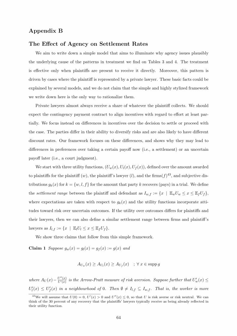
Appendix B

The Effect of Agency on Settlement Rates

We aim to write down a simple model that aims to illuminate why agency issues plausibly

the underlying cause of the patterns in treatment we find on Tables 3 and 4. The treatment

is effective only when plaintiffs are present to receive it directly. Moreover, this pattern is

driven by cases where the plaintiff is represented by a private lawyer. These basic facts could be

explained by several models, and we do not claim that the simple and highly stylized framework

we write down here is the only way to rationalize them.

Private lawyers almost always receive a share of whatever the plaintiff collects. We should

expect the contingency payment contract to align incentives with regard to effort at least par-

tially. We focus instead on differences in incentives over the decision to settle or proceed with

the case. The parties differ in their ability to diversify risks and are also likely to have different

discount rates. Our framework focuses on these differences, and shows why they may lead to

differences in preferences over taking a certain payoff now (i.e., a settlement) or an uncertain

payoff later (i.e., a court judgment).

We start with three utility functions, (Uw(x), Ul(x), Uf (x)), defined over the amount awarded

to plaintiffs for the plaintiff (w), the plaintiff’s lawyer (l), and the firms(f)43, and subjective dis-

tributions gk(x) for k = {w, l, f} for the amount that party k recovers (pays) in a trial. We define

the settlement range between the plaintiff and defendant as Iw,f := {x | EwUw ≤ x ≤ EfUf},

where expectations are taken with respect to gk(x) and the utility functions incorporate atti-

tudes toward risk over uncertain outcomes. If the utility over outcomes differs for plaintiffs and

their lawyers, then we can also define a similar settlement range between firms and plaintiff’s

lawyers as Il,f := {x | ElUl ≤ x ≤ EfUf}.

We show three claims that follow from this simple framework.

Claim 1 Suppose gw(x) = gl(x) = gf (x) := g(x) and

AUw(x) ≥ AUl(x) ≥ AUf

(x) ; ∀ x ∈ supp g

where AU (x)− U ′′(x)U ′(x) is the Arrow-Pratt measure of risk aversion. Suppose further that U ′w(x) ≤

U ′l (x) ≤ U ′f (x) in a neighbourhood of 0. Then ∅ 6= Il,f ⊆ Iw,f . That is, the worker is more

43We will assume that U(0) = 0, U ′(x) > 0 and U ′′(x) ≤ 0, so that U is risk averse or risk neutral. We canthink of the 30 percent of any recovery that the plaintiffs’ lawyers typically receive as being already reflected intheir utility function.

64

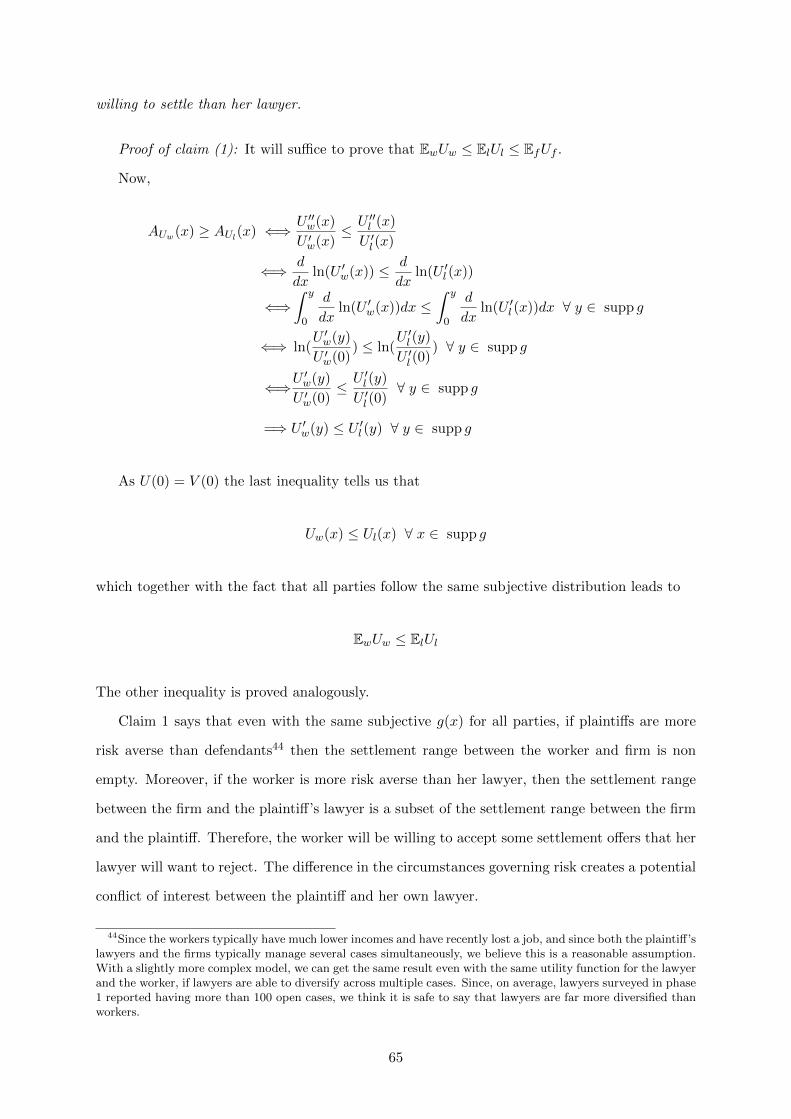
willing to settle than her lawyer.

Proof of claim (1): It will suffice to prove that EwUw ≤ ElUl ≤ EfUf .

Now,

AUw(x) ≥ AUl(x) ⇐⇒ U ′′w(x)

U ′w(x)≤U ′′l (x)

U ′l (x)

⇐⇒ d

dxln(U ′w(x)) ≤ d

dxln(U ′l (x))

⇐⇒∫ y

0

d

dxln(U ′w(x))dx ≤

∫ y

0

d

dxln(U ′l (x))dx ∀ y ∈ supp g

⇐⇒ ln(U ′w(y)

U ′w(0)) ≤ ln(

U ′l (y)

U ′l (0)) ∀ y ∈ supp g

⇐⇒U ′w(y)

U ′w(0)≤U ′l (y)

U ′l (0)∀ y ∈ supp g

=⇒ U ′w(y) ≤ U ′l (y) ∀ y ∈ supp g

As U(0) = V (0) the last inequality tells us that

Uw(x) ≤ Ul(x) ∀ x ∈ supp g

which together with the fact that all parties follow the same subjective distribution leads to

EwUw ≤ ElUl

The other inequality is proved analogously.

Claim 1 says that even with the same subjective g(x) for all parties, if plaintiffs are more

risk averse than defendants44 then the settlement range between the worker and firm is non

empty. Moreover, if the worker is more risk averse than her lawyer, then the settlement range

between the firm and the plaintiff’s lawyer is a subset of the settlement range between the firm

and the plaintiff. Therefore, the worker will be willing to accept some settlement offers that her

lawyer will want to reject. The difference in the circumstances governing risk creates a potential

conflict of interest between the plaintiff and her own lawyer.

44Since the workers typically have much lower incomes and have recently lost a job, and since both the plaintiff’slawyers and the firms typically manage several cases simultaneously, we believe this is a reasonable assumption.With a slightly more complex model, we can get the same result even with the same utility function for the lawyerand the worker, if lawyers are able to diversify across multiple cases. Since, on average, lawyers surveyed in phase1 reported having more than 100 open cases, we think it is safe to say that lawyers are far more diversified thanworkers.

65

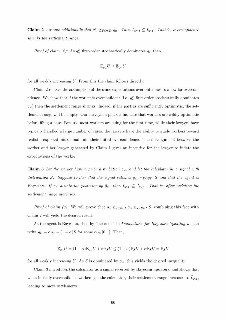
Claim 2 Assume additionally that gow �FOSD gw. Then Iwo,f ⊆ Iw,f . That is, overconfidence

shrinks the settlement range.

Proof of claim (2): As gow first-order stochastically dominates gw then

EgowU ≥ EgwU

for all weakly increasing U . From this the claim follows directly.

Claim 2 relaxes the assumption of the same expectations over outcomes to allow for overcon-

fidence. We show that if the worker is overconfident (i.e. gow first-order stochastically dominates

gw) then the settlement range shrinks. Indeed, if the parties are sufficiently optimistic, the set-

tlement range will be empty. Our surveys in phase 3 indicate that workers are wildly optimistic

before filing a case. Because most workers are suing for the first time, while their lawyers have

typically handled a large number of cases, the lawyers have the ability to guide workers toward

realistic expectations or maintain their initial overconfidence. The misalignment between the

worker and her lawyer generated by Claim 1 gives an incentive for the lawyer to inflate the

expectations of the worker.

Claim 3 Let the worker have a prior distribution gw, and let the calculator be a signal with

distribution S. Suppose further that the signal satisfies gw �FOSD S and that the agent is

Bayesian. If we denote the posterior by gw, then Iw,f ⊆ Iw,f . That is, after updating the

settlement range increases.

Proof of claim (3): We will prove that gw �FOSD gw �FOSD S, combining this fact with

Claim 2 will yield the desired result.

As the agent is Bayesian, then by Theorem 1 in Foundations for Bayesian Updating we can

write gw = αgw + (1− α)S for some α ∈ [0, 1]. Then,

EgwU = (1− α)EgwU + αESU ≤ (1− α)ESU + αESU = ESU

for all weakly increasing U . As S is dominated by gw, this yields the desired inequality.

Claim 3 introduces the calculator as a signal received by Bayesian updaters, and shows that

when initially overconfident workers get the calculator, their settlement range increases to Iw,f ,

leading to more settlements.

66

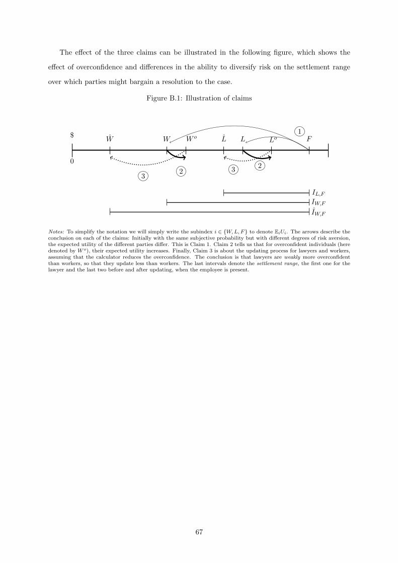
The effect of the three claims can be illustrated in the following figure, which shows the

effect of overconfidence and differences in the ability to diversify risk on the settlement range

over which parties might bargain a resolution to the case.

Figure B.1: Illustration of claims

$

0

W W W o L L Lo F1

22

33

IL,FIW,F

IW,F

Notes: To simplify the notation we will simply write the subindex i ∈ {W,L, F} to denote EiUi. The arrows describe theconclusion on each of the claims: Initially with the same subjective probability but with different degrees of risk aversion,the expected utility of the different parties differ. This is Claim 1. Claim 2 tells us that for overconfident individuals (heredenoted by W o), their expected utility increases. Finally, Claim 3 is about the updating process for lawyers and workers,assuming that the calculator reduces the overconfidence. The conclusion is that lawyers are weakly more overconfidentthan workers, so that they update less than workers. The last intervals denote the settlement range, the first one for thelawyer and the last two before and after updating, when the employee is present.

67

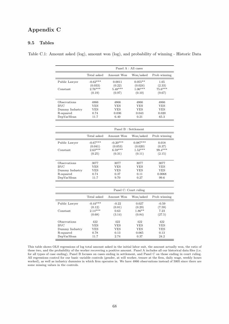
Appendix C

9.5 Tables

Table C.1: Amount asked (log), amount won (log), and probability of winning - Historic Data

Panel A : All cases

Total asked Amount Won Won/asked Prob winning

Public Lawyer -0.62*** 0.0011 0.055** 1.65(0.033) (0.22) (0.024) (2.33)

Constant 2.76*** 5.48*** 1.06*** 75.6***(0.19) (0.97) (0.10) (9.67)

Observations 4866 4866 4866 4866BVC YES YES YES YESDummy Industry YES YES YES YESR-squared 0.74 0.036 0.043 0.020DepVarMean 11.7 6.40 0.21 65.3

Panel B : Settlement

Total asked Amount Won Won/asked Prob winning

Public Lawyer -0.67*** -0.20*** 0.087*** 0.018(0.041) (0.053) (0.020) (0.37)

Constant 2.63*** 6.59*** 1.52*** 99.4***(0.25) (0.31) (0.11) (2.15)

Observations 3077 3077 3077 3077BVC YES YES YES YESDummy Industry YES YES YES YESR-squared 0.74 0.37 0.11 0.0068DepVarMean 11.7 9.70 0.27 99.6

Panel C: Court ruling

Total asked Amount Won Won/asked Prob winning

Public Lawyer -0.44*** -0.22 0.027 -0.59(0.12) (0.81) (0.29) (7.59)

Constant 2.14*** 0.63 1.86** 7.23(0.68) (3.14) (0.84) (27.5)

Observations 422 422 422 422BVC YES YES YES YESDummy Industry YES YES YES YESR-squared 0.78 0.13 0.065 0.13DepVarMean 11.7 2.74 0.37 24.2

This table shows OLS regressions of log total amount asked in the initial labor suit, the amount actually won, the ratio ofthese two, and the probability of the worker recovering a positive amount. Panel A includes all our historical data files (i.e.for all types of case ending), Panel B focuses on cases ending in settlement, and Panel C on those ending in court ruling.All regressions control for our basic variable controls (gender, at will worker, tenure at the firm, daily wage, weekly hoursworked), as well as industry dummies in which firm operates in. We have 4866 observations instead of 5005 since there aresome missing values in the controls.

68

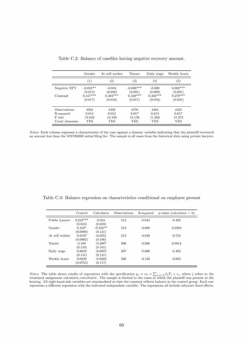
Table C.2: Balance of casefiles having negative recovery amount.

Gender At will worker Tenure Daily wage Weekly hours

(1) (2) (3) (4) (5)

Negative NPV -0.035** -0.034 -0.006*** -0.000 0.002***(0.014) (0.028) (0.001) (0.000) (0.001)

Constant 0.417*** 0.404*** 0.428*** 0.402*** 0.279***(0.017) (0.016) (0.017) (0.016) (0.035)

Observations 4503 4492 4470 4484 4425R-squared 0.014 0.013 0.017 0.013 0.017F stat 13.022 12.109 15.139 11.902 15.373Court dummies YES YES YES YES YES

Notes: Each column regresses a characteristic of the case against a dummy variable indicating that the plaintiff recoveredan amount less than the MXN$2000 initial filing fee. The sample is all cases from the historical data using private lawyers.

Table C.3: Balance regression on characteristics conditional on employee present

Control Calculator Observations R-squared p-value (calculator = 0)

Public Lawyer 0.223*** 0.034 312 0.042 0.492(0.043) (0.049)

Gender 0.162* -0.256** 312 0.080 0.0395(0.0890) (0.121)

At will worker 0.0197 -0.0351 312 0.049 0.742(0.0965) (0.106)

Tenure 0.189 -0.286* 306 0.068 0.0814(0.133) (0.161) .

Daily wage 0.0659 -0.0975 307 0.006 0.493(0.141) (0.141)

Weekly hours 0.0230 -0.0203 306 0.136 0.863(0.0755) (0.117)

Notes: The table shows results of regressions with the specification yi = αt +∑

j=1,2 βjTj + εi, where j refers to thetreatment assignment calculator, conciliator. The sample is limited to the cases in which the plaintiff was present at thehearing. All right-hand side variables are standardized so that the constant reflects balance in the control group. Each rowrepresents a different regression with the indicated independent variable. The regressions all include subcourt fixed effects.

69

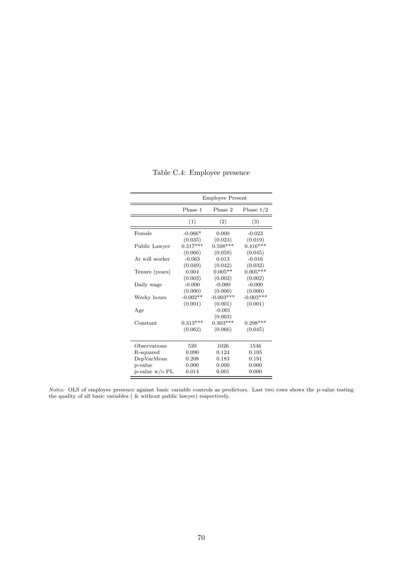
Table C.4: Employee presence

Employee Present

Phase 1 Phase 2 Phase 1/2

(1) (2) (3)

Female -0.066* 0.000 -0.023(0.035) (0.023) (0.019)

Public Lawyer 0.317*** 0.508*** 0.416***(0.066) (0.059) (0.045)

At will worker -0.063 0.013 -0.016(0.049) (0.042) (0.032)

Tenure (years) 0.004 0.005** 0.005***(0.003) (0.002) (0.002)

Daily wage -0.000 -0.000 -0.000(0.000) (0.000) (0.000)

Weeky hours -0.002** -0.003*** -0.003***(0.001) (0.001) (0.001)

Age -0.001(0.003)

Constant 0.313*** 0.303*** 0.298***(0.062) (0.066) (0.045)

Observations 520 1026 1546R-squared 0.090 0.124 0.105DepVarMean 0.208 0.183 0.191p-value 0.000 0.000 0.000p-value w/o PL 0.014 0.001 0.000

Notes: OLS of employee presence against basic variable controls as predictors. Last two rows shows the p-value testingthe quality of all basic variables ( & without public lawyer) respectively.

70

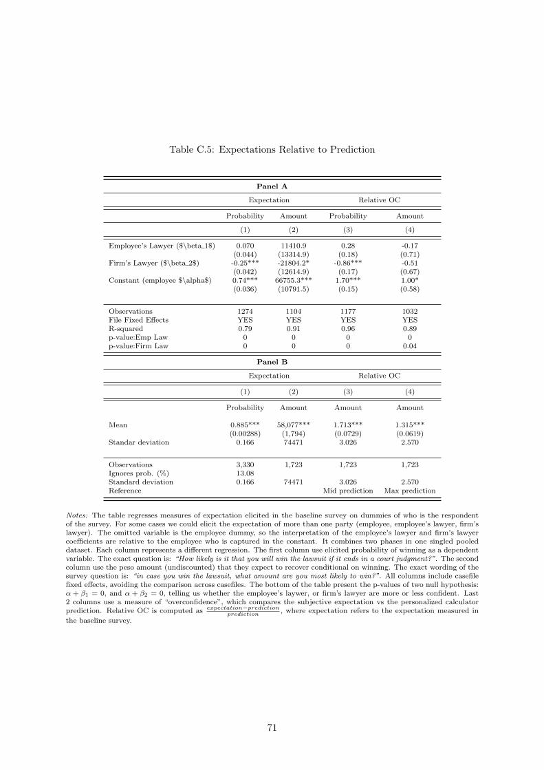
Table C.5: Expectations Relative to Prediction

Panel A

Expectation Relative OC

Probability Amount Probability Amount

(1) (2) (3) (4)

Employee’s Lawyer ($\beta 1$) 0.070 11410.9 0.28 -0.17(0.044) (13314.9) (0.18) (0.71)

Firm’s Lawyer ($\beta 2$) -0.25*** -21804.2* -0.86*** -0.51(0.042) (12614.9) (0.17) (0.67)

Constant (employee $\alpha$) 0.74*** 66755.3*** 1.70*** 1.00*(0.036) (10791.5) (0.15) (0.58)

Observations 1274 1104 1177 1032File Fixed Effects YES YES YES YESR-squared 0.79 0.91 0.96 0.89p-value:Emp Law 0 0 0 0p-value:Firm Law 0 0 0 0.04

Panel B

Expectation Relative OC

(1) (2) (3) (4)

Probability Amount Amount Amount

Mean 0.885*** 58,077*** 1.713*** 1.315***(0.00288) (1,794) (0.0729) (0.0619)

Standar deviation 0.166 74471 3.026 2.570

Observations 3,330 1,723 1,723 1,723Ignores prob. (%) 13.08Standard deviation 0.166 74471 3.026 2.570Reference Mid prediction Max prediction

Notes: The table regresses measures of expectation elicited in the baseline survey on dummies of who is the respondentof the survey. For some cases we could elicit the expectation of more than one party (employee, employee’s lawyer, firm’slawyer). The omitted variable is the employee dummy, so the interpretation of the employee’s lawyer and firm’s lawyercoefficients are relative to the employee who is captured in the constant. It combines two phases in one singled pooleddataset. Each column represents a different regression. The first column use elicited probability of winning as a dependentvariable. The exact question is: “How likely is it that you will win the lawsuit if it ends in a court judgment?”. The secondcolumn use the peso amount (undiscounted) that they expect to recover conditional on winning. The exact wording of thesurvey question is: “in case you win the lawsuit, what amount are you most likely to win?”. All columns include casefilefixed effects, avoiding the comparison across casefiles. The bottom of the table present the p-values of two null hypothesis:α + β1 = 0, and α + β2 = 0, telling us whether the employee’s laywer, or firm’s lawyer are more or less confident. Last2 columns use a measure of “overconfidence”, which compares the subjective expectation vs the personalized calculatorprediction. Relative OC is computed as expectation−prediction

prediction, where expectation refers to the expectation measured in

the baseline survey.

71

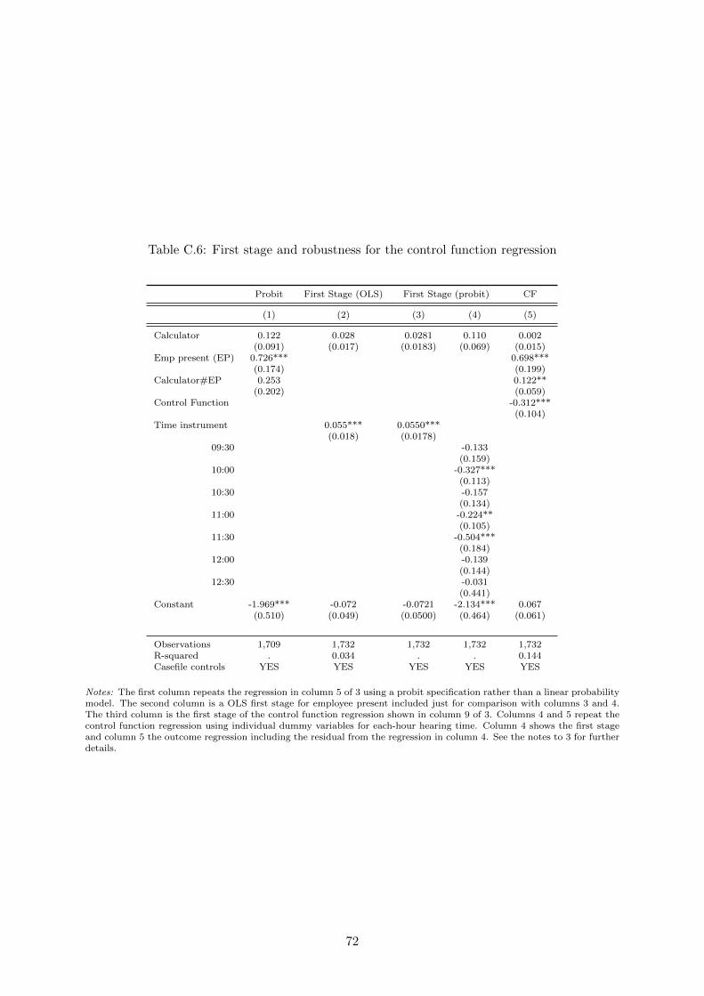
Table C.6: First stage and robustness for the control function regression

Probit First Stage (OLS) First Stage (probit) CF

(1) (2) (3) (4) (5)

Calculator 0.122 0.028 0.0281 0.110 0.002(0.091) (0.017) (0.0183) (0.069) (0.015)

Emp present (EP) 0.726*** 0.698***(0.174) (0.199)

Calculator#EP 0.253 0.122**(0.202) (0.059)

Control Function -0.312***(0.104)

Time instrument 0.055*** 0.0550***(0.018) (0.0178)

09:30 -0.133(0.159)

10:00 -0.327***(0.113)

10:30 -0.157(0.134)

11:00 -0.224**(0.105)

11:30 -0.504***(0.184)

12:00 -0.139(0.144)

12:30 -0.031(0.441)

Constant -1.969*** -0.072 -0.0721 -2.134*** 0.067(0.510) (0.049) (0.0500) (0.464) (0.061)

Observations 1,709 1,732 1,732 1,732 1,732R-squared . 0.034 . . 0.144Casefile controls YES YES YES YES YES

Notes: The first column repeats the regression in column 5 of 3 using a probit specification rather than a linear probabilitymodel. The second column is a OLS first stage for employee present included just for comparison with columns 3 and 4.The third column is the first stage of the control function regression shown in column 9 of 3. Columns 4 and 5 repeat thecontrol function regression using individual dummy variables for each-hour hearing time. Column 4 shows the first stageand column 5 the outcome regression including the residual from the regression in column 4. See the notes to 3 for furtherdetails.

72

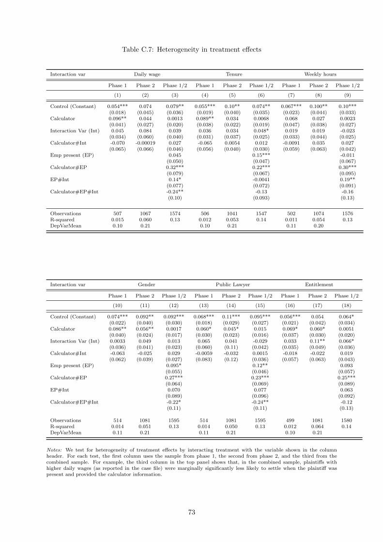
Table C.7: Heterogeneity in treatment effects

Interaction var Daily wage Tenure Weekly hours

Phase 1 Phase 2 Phase 1/2 Phase 1 Phase 2 Phase 1/2 Phase 1 Phase 2 Phase 1/2

(1) (2) (3) (4) (5) (6) (7) (8) (9)

Control (Constant) 0.054*** 0.074 0.079** 0.055*** 0.10** 0.074** 0.067*** 0.100** 0.10***(0.018) (0.045) (0.036) (0.019) (0.040) (0.035) (0.023) (0.044) (0.033)

Calculator 0.096** 0.044 0.0013 0.089** 0.034 0.0068 0.068 0.027 0.0023(0.041) (0.027) (0.020) (0.038) (0.022) (0.019) (0.047) (0.038) (0.027)

Interaction Var (Int) 0.045 0.084 0.039 0.036 0.034 0.048* 0.019 0.019 -0.023(0.034) (0.060) (0.040) (0.031) (0.037) (0.025) (0.033) (0.044) (0.025)

Calculator#Int -0.070 -0.00019 0.027 -0.065 0.0054 0.012 -0.0091 0.035 0.027(0.065) (0.066) (0.046) (0.056) (0.040) (0.030) (0.059) (0.063) (0.042)

Emp present (EP) 0.045 0.15*** -0.011(0.050) (0.047) (0.067)

Calculator#EP 0.32*** 0.22*** 0.30***(0.079) (0.067) (0.095)

EP#Int 0.14* -0.0041 0.19**(0.077) (0.072) (0.091)

Calculator#EP#Int -0.24** -0.13 -0.16(0.10) (0.093) (0.13)

Observations 507 1067 1574 506 1041 1547 502 1074 1576R-squared 0.015 0.060 0.13 0.012 0.053 0.14 0.011 0.054 0.13DepVarMean 0.10 0.21 0.10 0.21 0.11 0.20

Interaction var Gender Public Lawyer Entitlement

Phase 1 Phase 2 Phase 1/2 Phase 1 Phase 2 Phase 1/2 Phase 1 Phase 2 Phase 1/2

(10) (11) (12) (13) (14) (15) (16) (17) (18)

Control (Constant) 0.074*** 0.092** 0.092*** 0.068*** 0.11*** 0.095*** 0.056*** 0.054 0.064*(0.022) (0.040) (0.030) (0.018) (0.029) (0.027) (0.021) (0.042) (0.034)

Calculator 0.086** 0.056** 0.0017 0.060* 0.045* 0.015 0.069* 0.060* 0.0051(0.040) (0.024) (0.017) (0.030) (0.023) (0.016) (0.037) (0.030) (0.020)

Interaction Var (Int) 0.0033 0.049 0.013 0.065 0.041 -0.029 0.033 0.11** 0.066*(0.036) (0.041) (0.023) (0.060) (0.11) (0.042) (0.035) (0.049) (0.036)

Calculator#Int -0.063 -0.025 0.029 -0.0059 -0.032 0.0015 -0.018 -0.022 0.019(0.062) (0.039) (0.027) (0.083) (0.12) (0.036) (0.057) (0.063) (0.043)

Emp present (EP) 0.095* 0.12** 0.093(0.055) (0.046) (0.057)

Calculator#EP 0.27*** 0.23*** 0.25***(0.064) (0.069) (0.089)

EP#Int 0.070 0.077 0.063(0.089) (0.096) (0.092)

Calculator#EP#Int -0.22* -0.24** -0.12(0.11) (0.11) (0.13)

Observations 514 1081 1595 514 1081 1595 499 1081 1580R-squared 0.014 0.051 0.13 0.014 0.050 0.13 0.012 0.064 0.14DepVarMean 0.11 0.21 0.11 0.21 0.10 0.21

Notes: We test for heterogeneity of treatment effects by interacting treatment with the variable shown in the columnheader. For each test, the first column uses the sample from phase 1, the second from phase 2, and the third from thecombined sample. For example, the third column in the top panel shows that, in the combined sample, plaintiffs withhigher daily wages (as reported in the case file) were marginally significantly less likely to settle when the plaintiff waspresent and provided the calculator information.

73

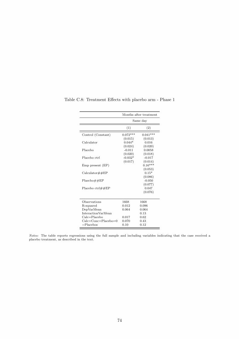
Table C.8: Treatment Effects with placebo arm - Phase 1

Months after treatment

Same day

(1) (2)

Control (Constant) 0.072*** 0.041***(0.015) (0.013)

Calculator 0.044* 0.016(0.024) (0.020)

Placebo -0.011 0.0058(0.020) (0.018)

Placebo ctrl -0.032* -0.017(0.017) (0.014)

Emp present (EP) 0.16***(0.053)

Calculator##EP 0.15*(0.086)

Plaecbo##EP -0.050(0.077)

Placebo ctrl##EP 0.047(0.076)

Observations 1668 1668R-squared 0.012 0.096DepVarMean 0.064 0.064InteractionVarMean 0.13Calc=Placebo 0.017 0.62Calc=Conc=Placebo=0 0.070 0.43=Placebos 0.10 0.12

Notes: The table reports regressions using the full sample and including variables indicating that the case received aplacebo treatment, as described in the text.

74

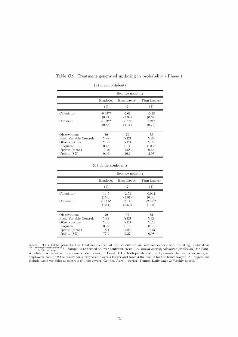
Table C.9: Treatment generated updating in probability - Phase 1

(a) Overconfidents

Relative updating

Employee Emp Lawyer Firm Lawyer

(1) (2) (3)

Calculator -0.45** 0.63 -0.48(0.21) (3.92) (0.62)

Constant -1.63** -15.9 1.24*(0.58) (11.1) (0.72)

Observations 30 79 58Basic Variable Controls YES YES YESOther controls YES YES YESR-squared 0.45 0.11 0.095Update (mean) -0.18 2.58 0.65Update (SD) 0.46 16.2 2.07

(b) Underconfidents

Relative updating

Employee Emp Lawyer Firm Lawyer

(1) (2) (3)

Calculator 14.5 -2.59 0.042(15.6) (1.97) (0.36)

Constant -167.5* 3.11 -2.46**(72.1) (5.50) (1.07)

Observations 20 56 32Basic Variable Controls YES YES YESOther controls YES YES YESR-squared 0.97 0.15 0.16Update (mean) 18.1 2.20 -0.23Update (SD) 77.9 9.27 0.98

Notes: This table presents the treatment effect of the calculator on relative expectation updating, defined asexitsurvey−initialsurvey

initialsurvey. Sample is restricted to over-confident cases (i.e. initial survey¿calculator prediction) for Panel

A, while it is restricted to under-confident cases for Panel B. For both panels, column 1 presents the results for surveyedemployees, column 2 the results for surveyed employee’s lawyer and table 3 the results for the firm’s lawyer. All regressionsinclude basic variables as controls (Public lawyer, Gender, At will worker, Tenure, Daily wage & Weekly hours).

75

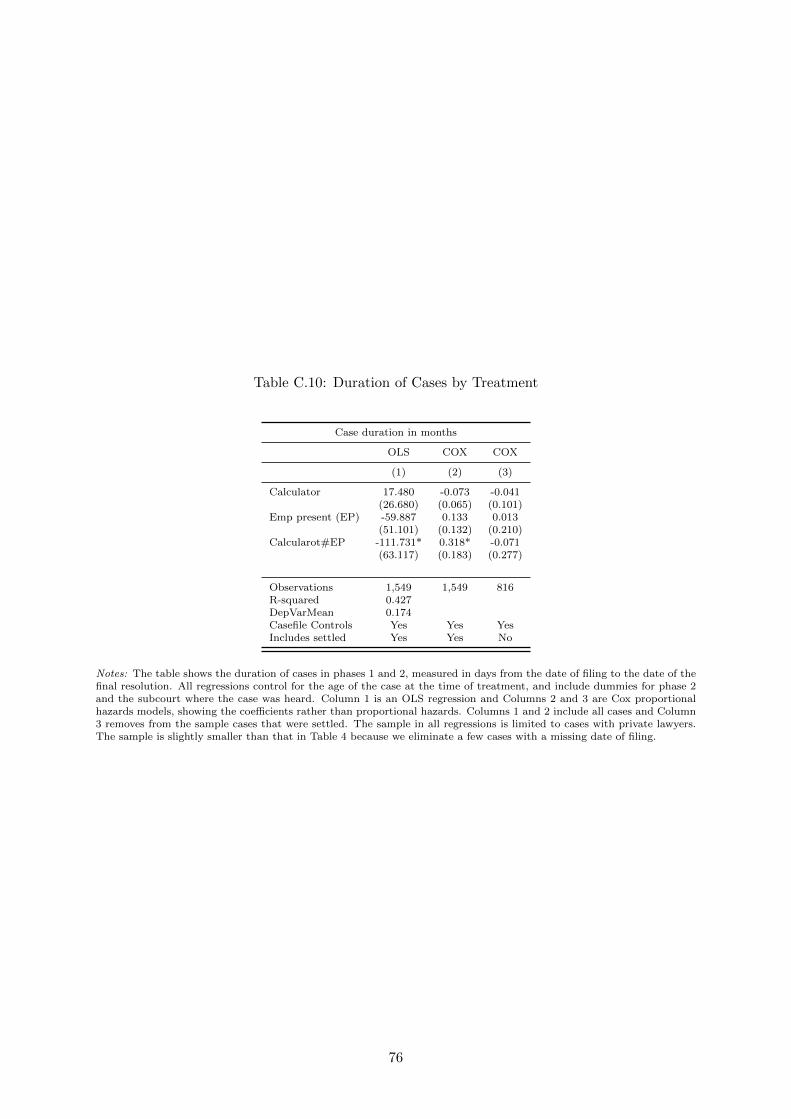
Table C.10: Duration of Cases by Treatment

Case duration in months

OLS COX COX

(1) (2) (3)

Calculator 17.480 -0.073 -0.041(26.680) (0.065) (0.101)

Emp present (EP) -59.887 0.133 0.013(51.101) (0.132) (0.210)

Calcularot#EP -111.731* 0.318* -0.071(63.117) (0.183) (0.277)

Observations 1,549 1,549 816R-squared 0.427DepVarMean 0.174Casefile Controls Yes Yes YesIncludes settled Yes Yes No

Notes: The table shows the duration of cases in phases 1 and 2, measured in days from the date of filing to the date of thefinal resolution. All regressions control for the age of the case at the time of treatment, and include dummies for phase 2and the subcourt where the case was heard. Column 1 is an OLS regression and Columns 2 and 3 are Cox proportionalhazards models, showing the coefficients rather than proportional hazards. Columns 1 and 2 include all cases and Column3 removes from the sample cases that were settled. The sample in all regressions is limited to cases with private lawyers.The sample is slightly smaller than that in Table 4 because we eliminate a few cases with a missing date of filing.

76

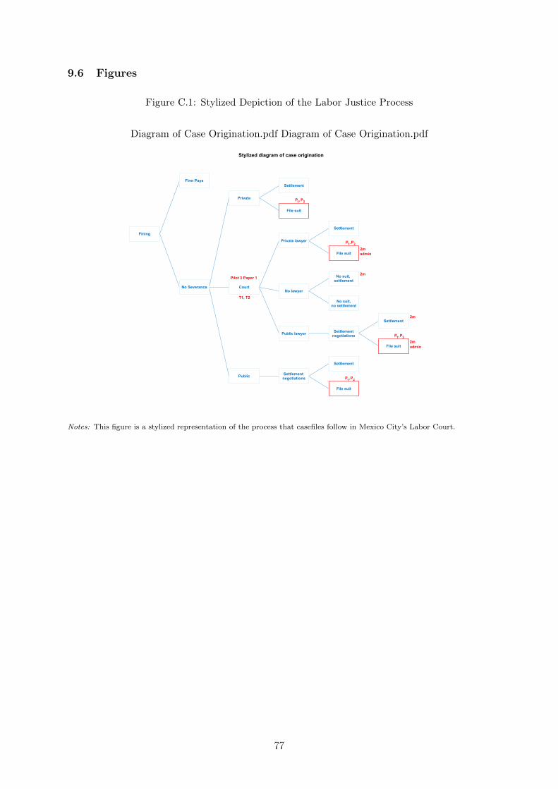
9.6 Figures

Figure C.1: Stylized Depiction of the Labor Justice Process

Diagram of Case Origination.pdf Diagram of Case Origination.pdf

Fining

No Severance

Firm Pays

Court

Public

Private

Settlement

File suit

Settlementnegotiations

Settlement

File suit

Private lawyer

Public lawyer

No lawyer

Settlement

File suit

No suit,settlement

No suit,no settlement

Settlementnegotiations

Settlement

File suit

P1, P2

P1, P2

P1, P2

P1, P2

2m

2m

2m

2madmin

admin

Pilot 3 Paper 1

T1, T2

Stylized diagram of case origination

Notes: This figure is a stylized representation of the process that casefiles follow in Mexico City’s Labor Court.

77

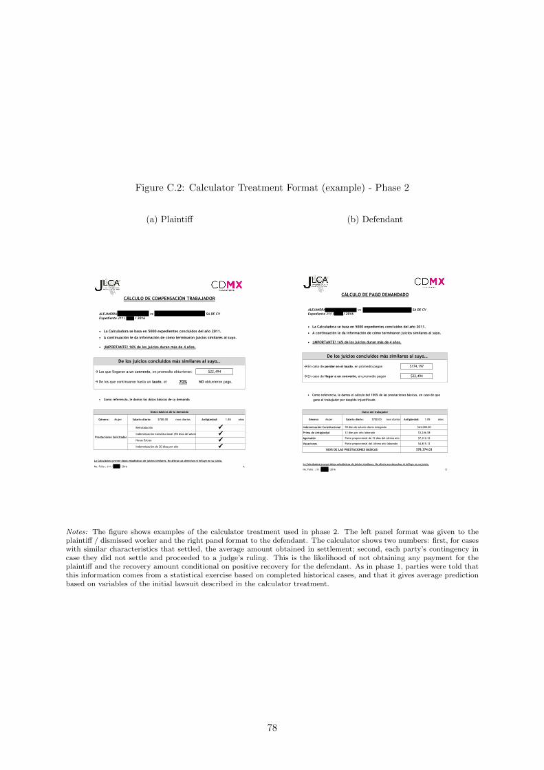
Figure C.2: Calculator Treatment Format (example) - Phase 2

(a) Plaintiff

• La Calculadora se basa en 5000 expedientes concluidos del año 2011.

• A continuación le da información de cómo terminaron juicios similares al suyo.

• ¡IMPORTANTE! 16% de los juicios duran más de 4 años.

ÆLos que llegaron a un convenio, en promedio obtuvieron:

ÆDe los que continuaron hasta un laudo, el 70% NO obtuvieron pago.

• Como referencia, le damos los datos básicos de su demanda

No. Folio : J11 / 2666 / 2016 A

PPPP

La Calculadora provee datos estadísticos de juicios similares. No afecta sus derechos ni influye en su juicio.

Reinstalación

Indemnización Constitucional (90 días de salario)

Horas Extras

Indemnización de 20 dias por año

Prestaciones Solicitadas

Expediente J11 / 2666 / 2016ALEJANDRA CHAVEZ GONZALEZ vs SERVICIOS Y ASESORIA VELARDE SA DE CV

CÁLCULO DE COMPENSACIÓN TRABAJADOR

Mujer añosSalario diario: $700.00 mxn diarios Antigüedad: 1.85

Datos básicos de la demanda

Género:

$22,494

De los juicios concluidos más similares al suyo…

(b) Defendant

• La Calculadora se basa en 5000 expedientes concluidos del año 2011.

• A continuación le da información de cómo terminaron juicios similares al suyo.

• ¡IMPORTANTE! 16% de los juicios duran más de 4 años.

ÆEn caso de perder en el laudo, en promedio pagan

ÆEn caso de llegar a un convenio, en promedio pagan

• Como referencia, le damos el cálculo del 100% de las prestaciones básicas, en caso de que

gane el trabajador por despido injustificado

La Calculadora provee datos estadísticos de juicios similares. No afecta sus derechos ni influye en su juicio.

1.85

Expediente J11 / 2666 / 2016

De los juicios concluidos más similares al suyo…

DNo. Folio : J11 / 2666 / 2016

$174,197

100% DE LAS PRESTACIONES BÁSICAS $78,374.03

años

Parte proporcional del último año laborado $4,815.12Vacaciones

$22,494

Parte proporcional de 15 días del último año $7,312.33

Indemnización Constitucional

Prima de Antigüedad

Aguinaldo

CÁLCULO DE PAGO DEMANDADO

90 días de salario diario integrado $63,000.00

12 días por año laborado $3,246.58

Datos del trabajador

Género: Mujer Salario diario: $700.00 mxn diarios Antigüedad:

ALEJANDRA CHAVEZ GONZALEZ vs SERVICIOS Y ASESORIA VELARDE SA DE CV

Notes: The figure shows examples of the calculator treatment used in phase 2. The left panel format was given to theplaintiff / dismissed worker and the right panel format to the defendant. The calculator shows two numbers: first, for caseswith similar characteristics that settled, the average amount obtained in settlement; second, each party’s contingency incase they did not settle and proceeded to a judge’s ruling. This is the likelihood of not obtaining any payment for theplaintiff and the recovery amount conditional on positive recovery for the defendant. As in phase 1, parties were told thatthis information comes from a statistical exercise based on completed historical cases, and that it gives average predictionbased on variables of the initial lawsuit described in the calculator treatment.

78

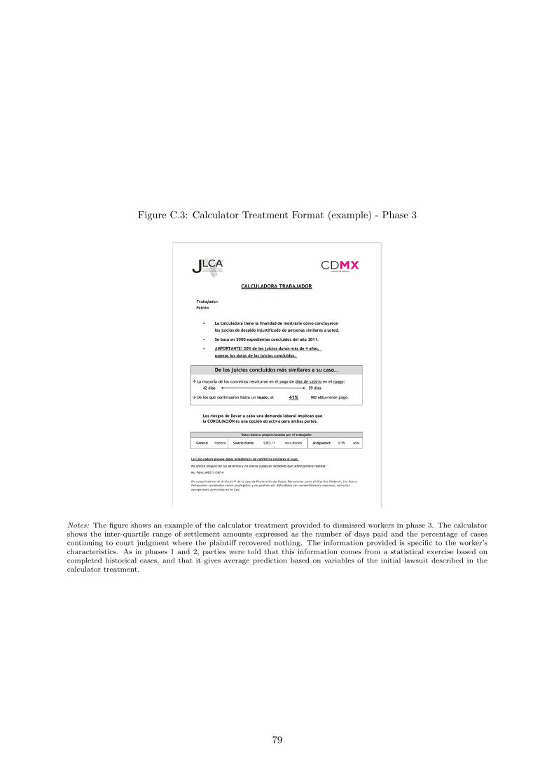
Figure C.3: Calculator Treatment Format (example) - Phase 3

Notes: The figure shows an example of the calculator treatment provided to dismissed workers in phase 3. The calculatorshows the inter-quartile range of settlement amounts expressed as the number of days paid and the percentage of casescontinuing to court judgment where the plaintiff recovered nothing. The information provided is specific to the worker’scharacteristics. As in phases 1 and 2, parties were told that this information comes from a statistical exercise based oncompleted historical cases, and that it gives average prediction based on variables of the initial lawsuit described in thecalculator treatment.

79

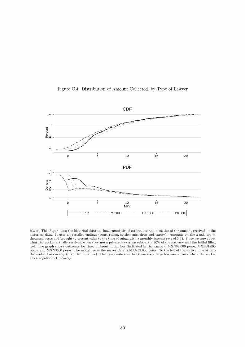
Figure C.4: Distribution of Amount Collected, by Type of Lawyer

.4.6

.81

Per

cent

0 5 10 15 20

CDF

0.0

5.1

.15

Den

sity

0 5 10 15 20NPV

Pub Pri 2000 Pri 1000 Pri 500

PDF

Notes: This Figure uses the historical data to show cumulative distributions and densities of the amount received in thehistorical data. It uses all casefiles endings (court ruling, settlements, drop and expiry). Amounts on the x-axis are inthousand pesos and brought to present value to the time of suing, with a monthly interest rate of 3.43. Since we care aboutwhat the worker actually receives, when they use a private lawyer we subtract a 30% of the recovery and the initial filingfeel. The graph shows outcomes for three different initial fees (indicated in the legend): MXN$2,000 pesos, MXN$1,000pesos, and MXN$500 pesos. The modal fee in the survey data is MXN$2,000 pesos. To the left of the vertical line at zerothe worker loses money (from the initial fee). The figure indicates that there are a large fraction of cases where the workerhas a negative net recovery.

80

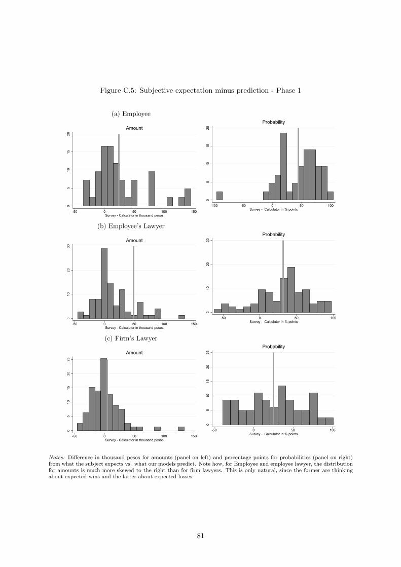
Figure C.5: Subjective expectation minus prediction - Phase 1

(a) Employee

05

1015

20

-50 0 50 100 150Survey - Calculator in thousand pesos

Amount

05

1015

20-100 -50 0 50 100

Survey - Calculator in % points

Probability

(b) Employee’s Lawyer

010

2030

-50 0 50 100 150Survey - Calculator in thousand pesos

Amount

010

2030

-50 0 50 100Survey - Calculator in % points

Probability

(c) Firm’s Lawyer

05

1015

2025

-50 0 50 100 150Survey - Calculator in thousand pesos

Amount

05

1015

2025

-50 0 50 100Survey - Calculator in % points

Probability

Notes: Difference in thousand pesos for amounts (panel on left) and percentage points for probabilities (panel on right)from what the subject expects vs. what our models predict. Note how, for Employee and employee lawyer, the distributionfor amounts is much more skewed to the right than for firm lawyers. This is only natural, since the former are thinkingabout expected wins and the latter about expected losses.

81

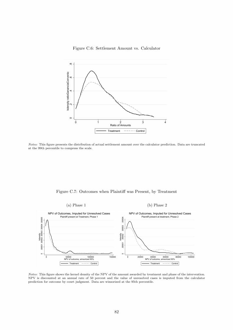
Figure C.6: Settlement Amount vs. Calculator

0.2

.4.6

.8kd

ensi

ty ra

tioG

anan

ciaC

onve

nio

0 1 2 3 4Ratio of Amounts

Treatment Control

Notes: This figure presents the distribution of actual settlement amount over the calculator prediction. Data are truncatedat the 99th percentile to compress the scale.

Figure C.7: Outcomes when Plaintiff was Present, by Treatment

(a) Phase 1

0.0

0001

.000

02.0

0003

.000

04.0

0005

kden

sity

0 50000 100000 150000NPV of outcome, winsorized 95%

Treatment Control

Plaintiff present at Treatment, Phase 1NPV of Outcomes, Imputed for Unresolved Cases

(b) Phase 2

0.0

0001

.000

02.0

0003

.000

04kd

ensi

ty

0 20000 40000 60000 80000 100000NPV of outcome, winsorized 95%

Treatment Control

Plaintiff present at treatment, Phase 2NPV of Outcomes, Imputed for Unresolved Cases

Notes: This figure shows the kernel density of the NPV of the amount awarded by treatment and phase of the intervention.NPV is discounted at an annual rate of 50 percent and the value of unresolved cases is imputed from the calculatorprediction for outcome by court judgment. Data are winsorized at the 95th percentile.

82

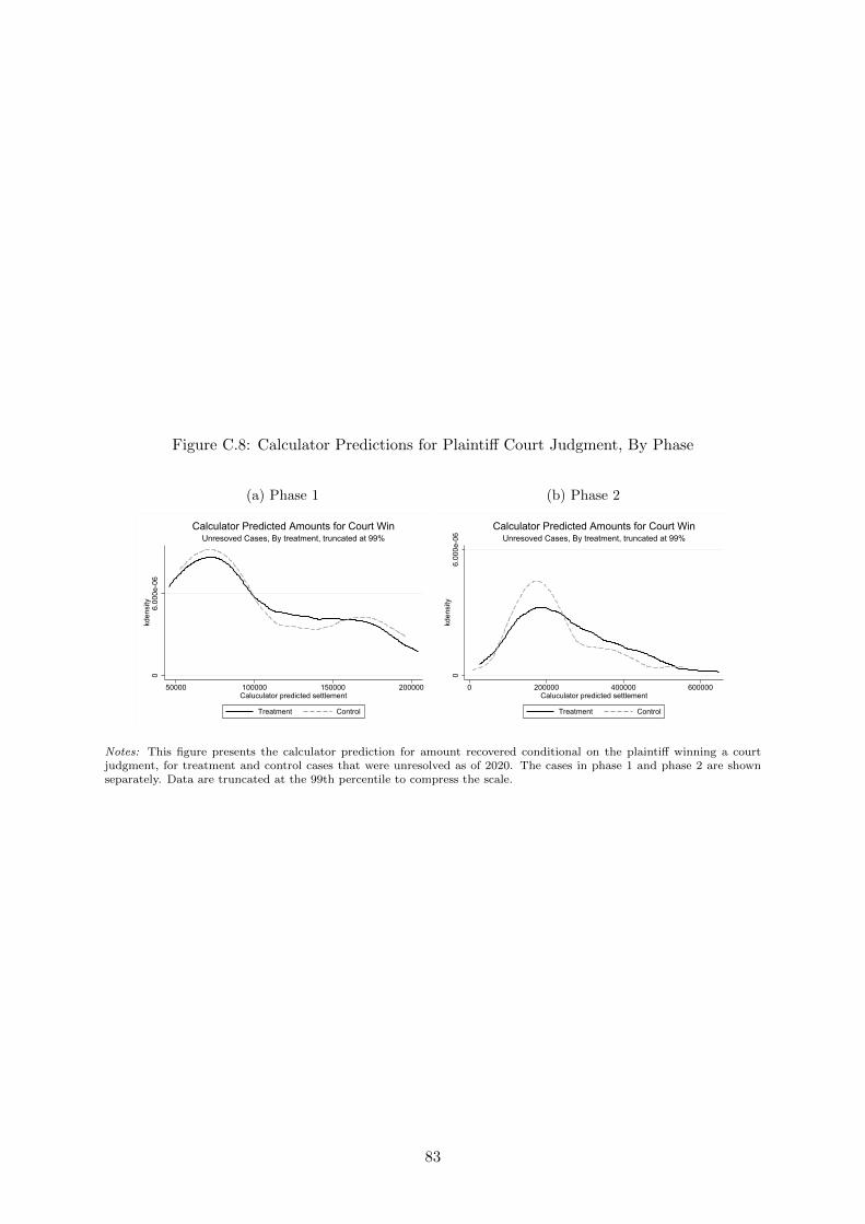
Figure C.8: Calculator Predictions for Plaintiff Court Judgment, By Phase

(a) Phase 1

06.

000e

-06

kden

sity

50000 100000 150000 200000Caluculator predicted settlement

Treatment Control

Unresoved Cases, By treatment, truncated at 99%Calculator Predicted Amounts for Court Win

(b) Phase 2

06.

000e

-06

kden

sity

0 200000 400000 600000Caluculator predicted settlement

Treatment Control

Unresoved Cases, By treatment, truncated at 99%Calculator Predicted Amounts for Court Win

Notes: This figure presents the calculator prediction for amount recovered conditional on the plaintiff winning a courtjudgment, for treatment and control cases that were unresolved as of 2020. The cases in phase 1 and phase 2 are shownseparately. Data are truncated at the 99th percentile to compress the scale.

83

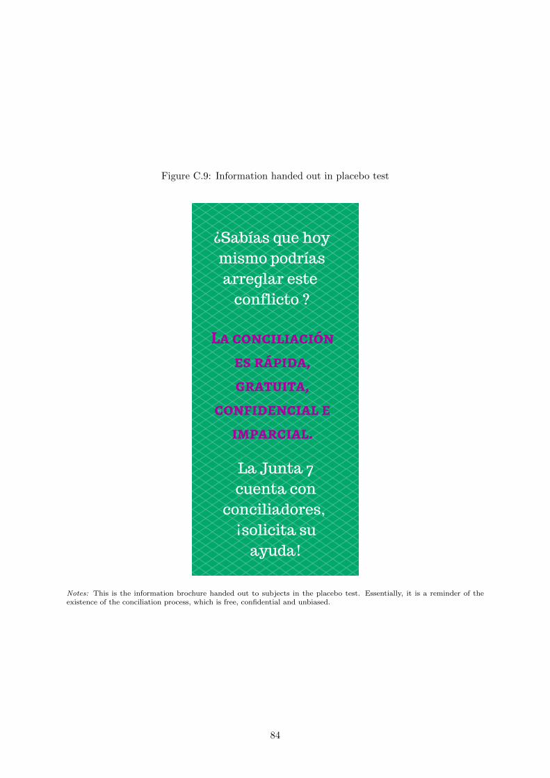
Figure C.9: Information handed out in placebo test

¿Sabías que hoy mismo podrías arreglar este

conflicto ?

La Junta 7 cuenta con

conciliadores, ¡solicita su

ayuda!

La conciliación

es rápida,

gratuita,

confidencial e

imparcial.

¿Sabías que hoy mismo podrías arreglar este

conflicto ?

La Junta 7 cuenta con

conciliadores, ¡solicita su

ayuda!

La conciliación

es rápida,

gratuita,

confidencial e

imparcial.

¿Sabías que hoy mismo podrías arreglar este

conflicto ?

La Junta 7 cuenta con

conciliadores, ¡solicita su

ayuda!

La conciliación

es rápida,

gratuita,

confidencial e

imparcial.

Notes: This is the information brochure handed out to subjects in the placebo test. Essentially, it is a reminder of theexistence of the conciliation process, which is free, confidential and unbiased.

84

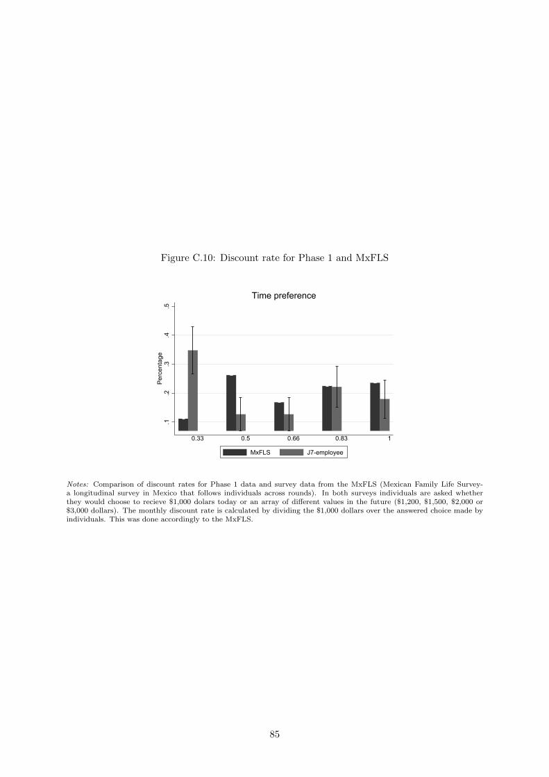
Figure C.10: Discount rate for Phase 1 and MxFLS

.1.2

.3.4

.5Pe

rcen

tage

0.33 0.5 0.66 0.83 1

MxFLS J7-employee

Time preference

Notes: Comparison of discount rates for Phase 1 data and survey data from the MxFLS (Mexican Family Life Survey-a longitudinal survey in Mexico that follows individuals across rounds). In both surveys individuals are asked whetherthey would choose to recieve $1,000 dolars today or an array of different values in the future ($1,200, $1,500, $2,000 or$3,000 dollars). The monthly discount rate is calculated by dividing the $1,000 dollars over the answered choice made byindividuals. This was done accordingly to the MxFLS.

85