Embed Size (px)
Citation preview
(Informal) Introduction to Stochastic Calculus
Paola Mosconi
Banca IMI
Bocconi University, 17-20/02/2017
Paola Mosconi 20541 – Lecture 1-2 1 / 65

Disclaimer
The opinion expressed here are solely those of the author and do not represent in
any way those of her employers
Paola Mosconi 20541 – Lecture 1-2 2 / 65
Main References
D. Brigo and F. Mercurio
Interest Rate Models – Theory and Practice. With Smile, Inflation and Credit
Springer (2006)
Appendix C
S. Shreve
Stochastic Calculus for Finance II
Springer (2004)
Chapters 1-6
Paola Mosconi 20541 – Lecture 1-2 3 / 65
From Deterministic to Stochastic Differential Equations
Outline
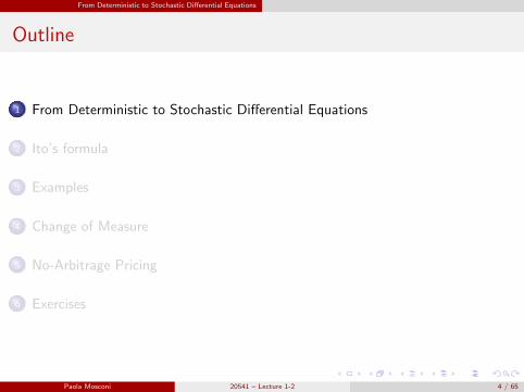
1 From Deterministic to Stochastic Differential Equations
2 Ito’s formula
3 Examples
4 Change of Measure
5 No-Arbitrage Pricing
6 Exercises
Paola Mosconi 20541 – Lecture 1-2 4 / 65
From Deterministic to Stochastic Differential Equations Probability Space
Preamble
[...] In continuous-time finance, we work within the framework of a probability space(Ω,F ,P). We normally have a fixed final time T, and then have a filtration, which is acollection of σ-algebras F(t); 0 ≤ t ≤ T, indexed by the time variable t. We interpretF(t) as the information available at time t. For 0 ≤ s ≤ t ≤ T, every set in F(s) is alsoin F(t). In other words, information increases over time. Within this context, an adaptedstochastic process is a collection of random variables X (t); 0 ≤ t ≤ T, also indexed bytime, such that for every t, X(t) is F(t)-measurable; the information at time t is sufficientto evaluate the random variable X (t). We think of X (t) as the price of some asset attime t and F(t) as the information obtained by watching all the prices in the market upto time t.Two important classes of adapted stochastic processes are martingales and Markov pro-cesses.
Shreve, Chapter 2
Paola Mosconi 20541 – Lecture 1-2 5 / 65
From Deterministic to Stochastic Differential Equations Probability Space
Probability Space: Definition
A probability space (Ω,F ,P) can be interpreted as an experiment, where:
ω ∈ Ω represents a generic result of the experiment
Ω is the set of all possible outcomes of the random experiment
a subset A ⊂ Ω represents an event
F is a collection of subsets of Ω which forms a σ-algebra (σ-field)
P is a probability measure
(See Shreve, Chapter 1)
Paola Mosconi 20541 – Lecture 1-2 6 / 65
From Deterministic to Stochastic Differential Equations Probability Space
Information
In order to price a derivative security in the no-arbitrage framework, we need tomodel mathematically the information on which our future decisions (contingencyplans) are based.
Given a non empty set Ω and a positive number T , assume that for eacht ∈ [0,T ] there is a σ-algebra Ft.Ft represents the information up to time t.
If t ≤ u, every set in Ft is also in Fu, i.e. Ft ⊆ Fu ⊆ F .“The information increases in time”, never exceeding the whole set of events
The family of σ-fields (Ft)t≥0 is called filtration.A filtration tells us the information that we will have at future times, i.e. when weget to time t we will know for each set in Ft whether the true ω lies in that set.
(See Shreve, Chapter 2)
Paola Mosconi 20541 – Lecture 1-2 7 / 65
From Deterministic to Stochastic Differential Equations Probability Space
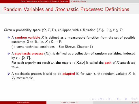
Random Variables and Stochastic Processes: Definitions
Given a probability space (Ω,F ,P), equipped with a filtration (Ft)t , 0 ≤ t ≤ T :
A random variable X is defined as a measurable function from the set of possibleoutcomes Ω to R, i.e. X : Ω → R
(+ some technical conditions – See Shreve, Chapter 1)
A stochastic process (Xt)t is defined as a collection of random variables, indexedby t ∈ [0,T ].
For each experiment result ω, the map t 7→ Xt(ω) is called the path of X associatedto ω.
A stochastic process is said to be adapted if, for each t, the random variable Xt isFt -measurable.
Paola Mosconi 20541 – Lecture 1-2 8 / 65
From Deterministic to Stochastic Differential Equations Probability Space
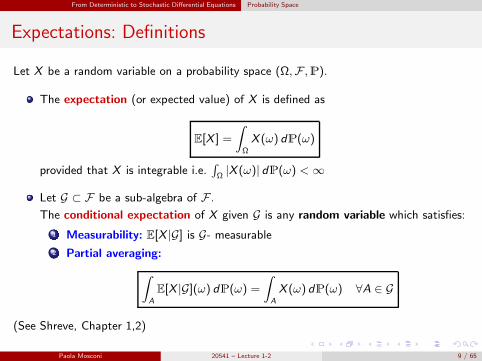
Expectations: Definitions
Let X be a random variable on a probability space (Ω,F ,P).
The expectation (or expected value) of X is defined as
E[X ] =
∫
Ω
X (ω) dP(ω)
provided that X is integrable i.e.∫
Ω|X (ω)| dP(ω) < ∞
Let G ⊂ F be a sub-algebra of F .
The conditional expectation of X given G is any random variable which satisfies:
1 Measurability: E[X |G] is G- measurable
2 Partial averaging:
∫
A
E[X |G](ω) dP(ω) =
∫
A
X (ω) dP(ω) ∀A ∈ G
(See Shreve, Chapter 1,2)
Paola Mosconi 20541 – Lecture 1-2 9 / 65
From Deterministic to Stochastic Differential Equations Probability Space
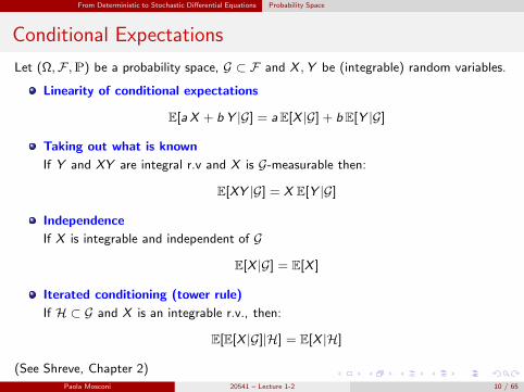
Conditional Expectations
Let (Ω,F ,P) be a probability space, G ⊂ F and X ,Y be (integrable) random variables.
Linearity of conditional expectations
E[a X + b Y |G] = aE[X |G] + bE[Y |G]
Taking out what is known
If Y and XY are integral r.v and X is G-measurable then:
E[XY |G] = X E[Y |G]
Independence
If X is integrable and independent of G
E[X |G] = E[X ]
Iterated conditioning (tower rule)
If H ⊂ G and X is an integrable r.v., then:
E[E[X |G]|H] = E[X |H]
(See Shreve, Chapter 2)Paola Mosconi 20541 – Lecture 1-2 10 / 65
From Deterministic to Stochastic Differential Equations Martingales
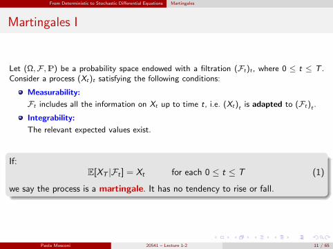
Martingales I
Let (Ω,F ,P) be a probability space endowed with a filtration (Ft)t , where 0 ≤ t ≤ T .Consider a process (Xt)t satisfying the following conditions:
Measurability:
Ft includes all the information on Xt up to time t, i.e. (Xt)t is adapted to (Ft)t .
Integrability:
The relevant expected values exist.
If:E[XT |Ft ] = Xt for each 0 ≤ t ≤ T (1)
we say the process is a martingale. It has no tendency to rise or fall.
Paola Mosconi 20541 – Lecture 1-2 11 / 65
From Deterministic to Stochastic Differential Equations Martingales
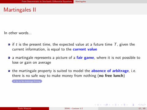
Martingales II
In other words...
if t is the present time, the expected value at a future time T , given thecurrent information, is equal to the current value
a martingale represents a picture of a fair game, where it is not possible tolose or gain on average
the martingale property is suited to model the absence of arbitrage, i.e.there is no safe way to make money from nothing (no free lunch)
Go to No-Arbitrage Pricing
Paola Mosconi 20541 – Lecture 1-2 12 / 65
From Deterministic to Stochastic Differential Equations Martingales
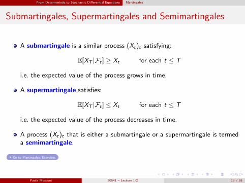
Submartingales, Supermartingales and Semimartingales
A submartingale is a similar process (Xt)t satisfying:
E[XT |Ft ] ≥ Xt for each t ≤ T
i.e. the expected value of the process grows in time.
A supermartingale satisfies:
E[XT |Ft ] ≤ Xt for each t ≤ T
i.e. the expected value of the process decreases in time.
A process (Xt)t that is either a submartingale or a supermartingale is termeda semimartingale.
Go to Martingales: Exercises
Paola Mosconi 20541 – Lecture 1-2 13 / 65
From Deterministic to Stochastic Differential Equations Variations/Covariantions
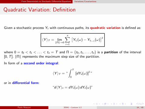
Quadratic Variation: Definition
Given a stochastic process Yt with continuous paths, its quadratic variation is defined as:
〈Y 〉T = lim‖Π‖→0
n∑
i=1
[
Yti (ω)− Yti−1 (ω)]2
where 0 = t0 < t1 < . . . < tn = T and Π = t0, t1, . . . , tn is a partition of the interval[0,T ]. ‖Π‖ represents the maximum step size of the partition.
In form of a second order integral:
〈Y 〉T = “
∫ T
0
[dYs(ω)]2 ”
or in differential form:“d〈Y 〉t = dYt(ω) dYt(ω)”
Paola Mosconi 20541 – Lecture 1-2 14 / 65
From Deterministic to Stochastic Differential Equations Variations/Covariantions
Quadratic Variation: Deterministic Process
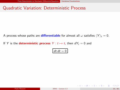
A process whose paths are differentiable for almost all ω satisfies 〈Y 〉t = 0.
If Y is the deterministic process Y : t 7→ t, then dYt = 0 and
dt dt = 0
Paola Mosconi 20541 – Lecture 1-2 15 / 65
From Deterministic to Stochastic Differential Equations Variations/Covariantions
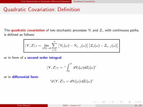
Quadratic Covariation: Definition
The quadratic covariation of two stochastic processes Yt and Zt , with continuous paths,is defined as follows:
〈Y ,Z 〉T = lim‖Π‖→0
n∑
i=1
[
Yti (ω)− Yti−1(ω)] [
Zti (ω)− Zti−1(ω)]
or in form of a second order integral:
〈Y ,Z 〉T = “
∫ T
0
dYs(ω)dZs(ω)”
or in differential form:“d〈Y ,Z 〉t = dYt(ω) dZt(ω)”
Paola Mosconi 20541 – Lecture 1-2 16 / 65
From Deterministic to Stochastic Differential Equations Deterministic Differential Equations
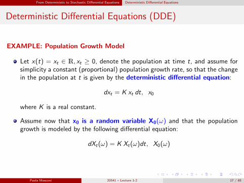
Deterministic Differential Equations (DDE)
EXAMPLE: Population Growth Model
Let x(t) = xt ∈ R, xt ≥ 0, denote the population at time t, and assume forsimplicity a constant (proportional) population growth rate, so that the changein the population at t is given by the deterministic differential equation:
dxt = K xt dt, x0
where K is a real constant.
Assume now that x0 is a random variable X0(ω) and that the populationgrowth is modeled by the following differential equation:
dXt(ω) = K Xt(ω)dt, X0(ω)
Paola Mosconi 20541 – Lecture 1-2 17 / 65
From Deterministic to Stochastic Differential Equations Deterministic Differential Equations
From Deterministic to Stochastic Differential Equations
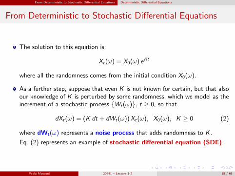
The solution to this equation is:
Xt(ω) = X0(ω) eKt
where all the randomness comes from the initial condition X0(ω).
As a further step, suppose that even K is not known for certain, but that alsoour knowledge of K is perturbed by some randomness, which we model as theincrement of a stochastic process Wt(ω), t ≥ 0, so that
dXt(ω) = (K dt + dWt(ω))Xt(ω), X0(ω), K ≥ 0 (2)
where dWt(ω) represents a noise process that adds randomness to K .
Eq. (2) represents an example of stochastic differential equation (SDE).
Paola Mosconi 20541 – Lecture 1-2 18 / 65
From Deterministic to Stochastic Differential Equations Stochastic Differential Equations
Stochastic Differential Equations (SDE)
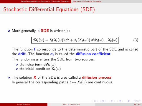
More generally, a SDE is written as
dXt(ω) = ft(Xt(ω)) dt + σt(Xt(ω)) dWt(ω), X0(ω) (3)
The function f corresponds to the deterministic part of the SDE and is calledthe drift. The function σt is called the diffusion coefficient.
The randomness enters the SDE from two sources:
the noise term dWt(ω)the initial condition X0(ω)
The solution X of the SDE is also called a diffusion process.In general the corresponding paths t 7→ Xt(ω) are continuous.
Paola Mosconi 20541 – Lecture 1-2 19 / 65
From Deterministic to Stochastic Differential Equations Stochastic Differential Equations
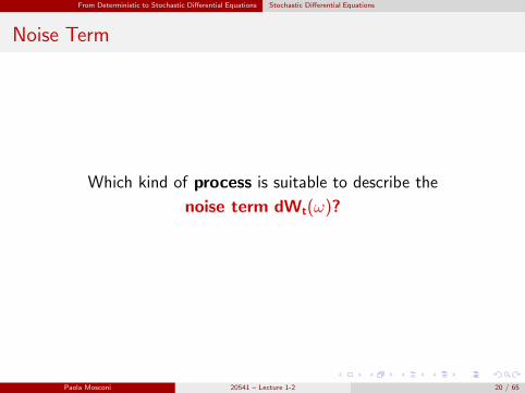
Noise Term
Which kind of process is suitable to describe the
noise term dWt(ω)?
Paola Mosconi 20541 – Lecture 1-2 20 / 65
From Deterministic to Stochastic Differential Equations Brownian Motion
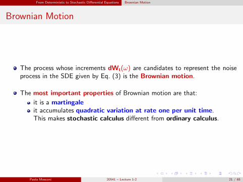
Brownian Motion
The process whose increments dWt(ω) are candidates to represent the noiseprocess in the SDE given by Eq. (3) is the Brownian motion.
The most important properties of Brownian motion are that:
it is a martingaleit accumulates quadratic variation at rate one per unit time.This makes stochastic calculus different from ordinary calculus.
Paola Mosconi 20541 – Lecture 1-2 21 / 65
From Deterministic to Stochastic Differential Equations Brownian Motion
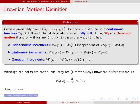
Brownian Motion: Definition
Definition
Given a probability space (Ω,F , (Ft)t ,P), for each ω ∈ Ω there is a continuousfunction Wt , t ≥ 0 such that it depends on ω and W0 = 0. Then, Wt is a Brownianmotion if and only if for any 0 < s < t < u and any h > 0 it has:
Independent increments: Wu(ω)−Wt(ω) independent of Wt(ω)−Ws(ω)
Stationary increments: Wt+h(ω)−Ws+h(ω) ∼ Wt(ω)−Ws(ω)
Gaussian increments: Wt(ω)−Ws(ω) ∼ N (0, t − s)
Although the paths are continuous, they are (almost surely) nowhere differentiable, i.e.
Wt(ω) =d
dtWt(ω)
does not exist.
Go to Brownian Motion: Exercises
Paola Mosconi 20541 – Lecture 1-2 22 / 65
From Deterministic to Stochastic Differential Equations Brownian Motion
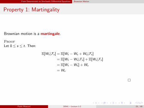
Property 1: Martingality
Brownian motion is a martingale.
Proof
Let 0 ≤ s ≤ t. Then:
E[Wt |Fs ] = E[Wt −Ws +Ws |Fs ]
= E[Wt −Ws |Fs ] + E[Ws |Fs ]
= E[Wt −Ws ] +Ws
= Ws
Paola Mosconi 20541 – Lecture 1-2 23 / 65
From Deterministic to Stochastic Differential Equations Brownian Motion
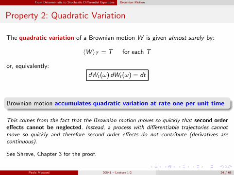
Property 2: Quadratic Variation
The quadratic variation of a Brownian motion W is given almost surely by:
〈W 〉T = T for each T
or, equivalently:
dWt(ω) dWt(ω) = dt
Brownian motion accumulates quadratic variation at rate one per unit time
This comes from the fact that the Brownian motion moves so quickly that second ordereffects cannot be neglected. Instead, a process with differentiable trajectories cannotmove so quickly and therefore second order effects do not contribute (derivatives arecontinuous).
See Shreve, Chapter 3 for the proof.
Paola Mosconi 20541 – Lecture 1-2 24 / 65
From Deterministic to Stochastic Differential Equations Brownian Motion
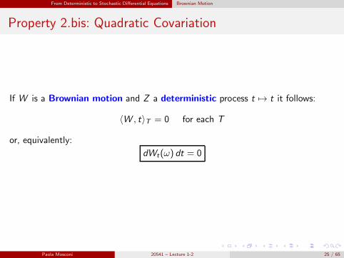
Property 2.bis: Quadratic Covariation
If W is a Brownian motion and Z a deterministic process t 7→ t it follows:
〈W , t〉T = 0 for each T
or, equivalently:
dWt(ω) dt = 0
Paola Mosconi 20541 – Lecture 1-2 25 / 65
From Deterministic to Stochastic Differential Equations Stochastic Integrals
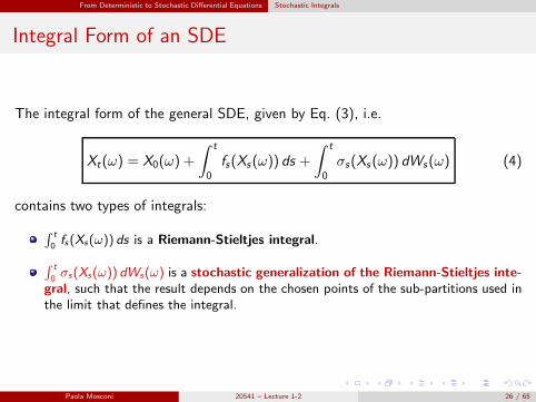
Integral Form of an SDE
The integral form of the general SDE, given by Eq. (3), i.e.
Xt(ω) = X0(ω) +
∫ t
0
fs(Xs(ω)) ds +
∫ t
0
σs(Xs(ω)) dWs(ω) (4)
contains two types of integrals:
∫ t
0fs(Xs(ω)) ds is a Riemann-Stieltjes integral.
∫ t
0σs(Xs(ω)) dWs(ω) is a stochastic generalization of the Riemann-Stieltjes inte-
gral, such that the result depends on the chosen points of the sub-partitions used inthe limit that defines the integral.
Paola Mosconi 20541 – Lecture 1-2 26 / 65
From Deterministic to Stochastic Differential Equations Stochastic Integrals
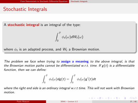
Stochastic Integrals
A stochastic integral is an integral of the type:
∫ T
0
φt(ω)dWt(ω)
where φt is an adapted process, and Wt a Brownian motion.
The problem we face when trying to assign a meaning to the above integral, is thatthe Brownian motion paths cannot be differentiated w.r.t. time. If g(t) is a differentiablefunction, then we can define:
∫ T
0
φt(ω)dg(t) =
∫ T
0
φt(ω)g′(t)dt
where the right end side is an ordinary integral w.r.t time. This will not work with Brownianmotion.
Paola Mosconi 20541 – Lecture 1-2 27 / 65
From Deterministic to Stochastic Differential Equations Stochastic Integrals
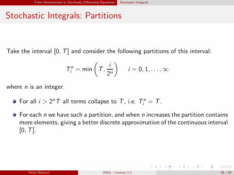
Stochastic Integrals: Partitions
Take the interval [0,T ] and consider the following partitions of this interval:
T ni = min
(
T ,i
2n
)
i = 0, 1, . . . ,∞
where n is an integer.
For all i > 2nT all terms collapse to T , i.e. T ni = T .
For each n we have such a partition, and when n increases the partition containsmore elements, giving a better discrete approximation of the continuous interval[0,T ].
Paola Mosconi 20541 – Lecture 1-2 28 / 65
From Deterministic to Stochastic Differential Equations Stochastic Integrals
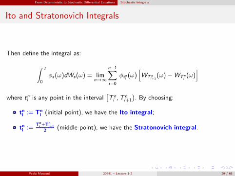
Ito and Stratonovich Integrals
Then define the integral as:
∫ T
0
φs(ω)dWs(ω) = limn→∞
n−1∑
i=0
φtni(ω)
[
WT ni+1(ω)−WT n
i(ω)
]
where tni is any point in the interval[
T ni ,T
ni+1
)
. By choosing:
tni := Tni (initial point), we have the Ito integral;
tni :=Tn
i +Tni+1
2 (middle point), we have the Stratonovich integral.
Paola Mosconi 20541 – Lecture 1-2 29 / 65
From Deterministic to Stochastic Differential Equations Stochastic Integrals
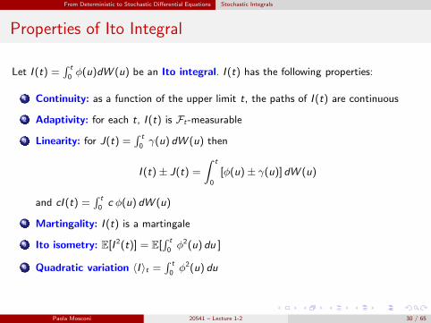
Properties of Ito Integral
Let I (t) =∫ t
0φ(u)dW (u) be an Ito integral. I (t) has the following properties:
1 Continuity: as a function of the upper limit t, the paths of I (t) are continuous
2 Adaptivity: for each t, I (t) is Ft-measurable
3 Linearity: for J(t) =∫ t
0γ(u) dW (u) then
I (t) ± J(t) =
∫ t
0
[φ(u)± γ(u)]dW (u)
and cI (t) =∫ t
0c φ(u) dW (u)
4 Martingality: I (t) is a martingale
5 Ito isometry: E[I 2(t)] = E[∫ t
0φ2(u) du ]
6 Quadratic variation 〈I 〉t =∫ t
0φ2(u) du
Paola Mosconi 20541 – Lecture 1-2 30 / 65
From Deterministic to Stochastic Differential Equations Stochastic Integrals
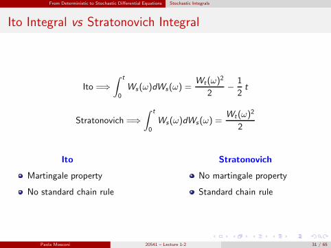
Ito Integral vs Stratonovich Integral
Ito =⇒∫ t
0
Ws(ω)dWs(ω) =Wt(ω)
2
2− 1
2t
Stratonovich =⇒∫ t
0
Ws(ω)dWs(ω) =Wt(ω)
2
2
Ito
Martingale property
No standard chain rule
Stratonovich
No martingale property
Standard chain rule
Paola Mosconi 20541 – Lecture 1-2 31 / 65
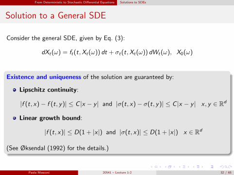
From Deterministic to Stochastic Differential Equations Solutions to SDEs
Solution to a General SDE
Consider the general SDE, given by Eq. (3):
dXt(ω) = ft(t,Xt(ω)) dt + σt(t,Xt(ω)) dWt(ω), X0(ω)
Existence and uniqueness of the solution are guaranteed by:
Lipschitz continuity:
|f (t, x)− f (t, y)| ≤ C |x − y | and |σ(t, x)− σ(t, y)| ≤ C |x − y | x , y ∈ Rd
Linear growth bound:
|f (t, x)| ≤ D(1 + |x |) and |σ(t, x)| ≤ D(1 + |x |) x ∈ Rd
(See Øksendal (1992) for the details.)
Paola Mosconi 20541 – Lecture 1-2 32 / 65
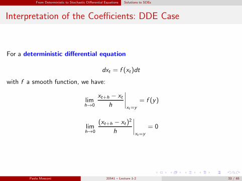
From Deterministic to Stochastic Differential Equations Solutions to SDEs
Interpretation of the Coefficients: DDE Case
For a deterministic differential equation
dxt = f (xt)dt
with f a smooth function, we have:
limh→0
xt+h − xt
h
∣
∣
∣
∣
xt=y
= f (y)
limh→0
(xt+h − xt)2
h
∣
∣
∣
∣
xt=y
= 0
Paola Mosconi 20541 – Lecture 1-2 33 / 65
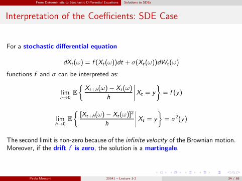
From Deterministic to Stochastic Differential Equations Solutions to SDEs
Interpretation of the Coefficients: SDE Case
For a stochastic differential equation
dXt(ω) = f (Xt(ω))dt + σ(Xt (ω))dWt(ω)
functions f and σ can be interpreted as:
limh→0
E
Xt+h(ω)− Xt(ω)
h
∣
∣
∣
∣
Xt = y
= f (y)
limh→0
E
[Xt+h(ω)− Xt(ω)]2
h
∣
∣
∣
∣
Xt = y
= σ2(y)
The second limit is non-zero because of the infinite velocity of the Brownian motion.Moreover, if the drift f is zero, the solution is a martingale.
Paola Mosconi 20541 – Lecture 1-2 34 / 65
Ito’s formula
Outline
1 From Deterministic to Stochastic Differential Equations
2 Ito’s formula
3 Examples
4 Change of Measure
5 No-Arbitrage Pricing
6 Exercises
Paola Mosconi 20541 – Lecture 1-2 35 / 65

Ito’s formula Chain Rule
Deterministic Case
For a deterministic differential equation such as
dxt = f (xt)dt
given a smooth transformation φ(t, x), we can write the evolution of φ(t, xt ) viathe standard chain rule:
dφ(t, xt) =∂φ
∂t(t, xt)dt +
∂φ
∂x(t, xt)dxt (5)
Paola Mosconi 20541 – Lecture 1-2 36 / 65
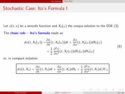
Ito’s formula Chain Rule
Stochastic Case: Ito’s Formula I
Let φ(t, x) be a smooth function and Xt(ω) the unique solution to the SDE (3).
The chain rule – Ito’s formula reads as:
dφ(t,Xt(ω)) =∂φ
∂t(t,Xt(ω))dt +
∂φ
∂x(t,Xt(ω))dXt (ω)
+1
2
∂2φ
∂x2(t,Xt(ω))dXt(ω)dXt(ω)
(6)
or, in compact notation:
dφ(t,Xt) =∂φ
∂t(t,Xt)dt +
∂φ
∂x(t,Xt)dXt +
1
2
∂2φ
∂x2(t,Xt)d〈X 〉t
Paola Mosconi 20541 – Lecture 1-2 37 / 65
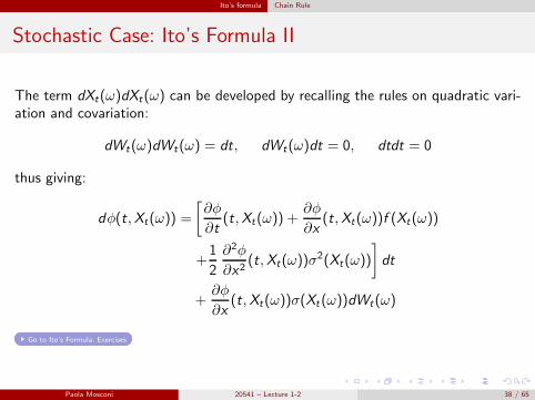
Ito’s formula Chain Rule
Stochastic Case: Ito’s Formula II
The term dXt(ω)dXt(ω) can be developed by recalling the rules on quadratic vari-ation and covariation:
dWt(ω)dWt(ω) = dt, dWt(ω)dt = 0, dtdt = 0
thus giving:
dφ(t,Xt(ω)) =
[
∂φ
∂t(t,Xt(ω)) +
∂φ
∂x(t,Xt(ω))f (Xt(ω))
+1
2
∂2φ
∂x2(t,Xt(ω))σ
2(Xt(ω))
]
dt
+∂φ
∂x(t,Xt(ω))σ(Xt (ω))dWt(ω)
Go to Ito’s Formula: Exercises
Paola Mosconi 20541 – Lecture 1-2 38 / 65
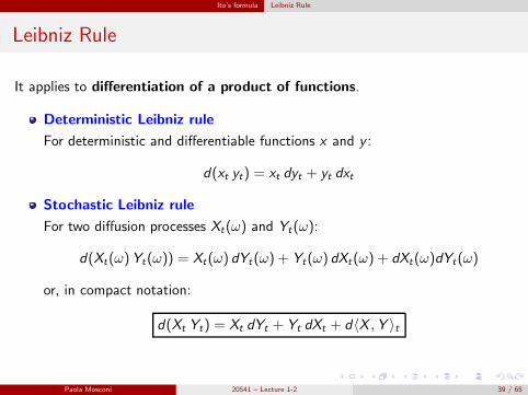
Ito’s formula Leibniz Rule
Leibniz Rule
It applies to differentiation of a product of functions.
Deterministic Leibniz rule
For deterministic and differentiable functions x and y :
d(xt yt) = xt dyt + yt dxt
Stochastic Leibniz rule
For two diffusion processes Xt(ω) and Yt(ω):
d(Xt(ω)Yt(ω)) = Xt(ω) dYt(ω) + Yt(ω) dXt(ω) + dXt(ω)dYt(ω)
or, in compact notation:
d(Xt Yt) = Xt dYt + Yt dXt + d〈X ,Y 〉t
Paola Mosconi 20541 – Lecture 1-2 39 / 65

Examples
Outline
1 From Deterministic to Stochastic Differential Equations
2 Ito’s formula
3 Examples
4 Change of Measure
5 No-Arbitrage Pricing
6 Exercises
Paola Mosconi 20541 – Lecture 1-2 40 / 65
Examples Linear SDE
Linear SDE with Deterministic Diffusion Coefficient I
A SDE is linear if both its drift and diffusion coefficients are first order polynomialsin the state variable.
Consider the particular case:
dXt(ω) = (αt + βtXt(ω)) dt + vtdWt(ω), X0(ω) = x0 (7)
where α, β, v are deterministic functions of time, regular enough to ensure existenceand uniqueness of the solution.
The solution is:
Xt(ω) = e∫
t
0βsds
[
x0 +
∫ t
0
e−∫
s
0βudu αs ds +
∫ t
0
e−∫
s
0βudu vs dWs(ω)
]
= x0e∫
t
0βsds +
∫ t
0
e∫
t
sβudu αs ds +
∫ t
0
e∫
t
sβudu vs dWs(ω)
(8)
Paola Mosconi 20541 – Lecture 1-2 41 / 65
Examples Linear SDE
Linear SDE with Deterministic Diffusion Coefficient II
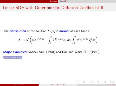
The distribution of the solution Xt(ω) is normal at each time t:
Xt ∼ N(
x0e∫
t
0βsds +
∫ t
0
e∫
t
sβudu αs ds,
∫ t
0
e2∫
t
sβudu v2
s ds
)
Major examples: Vasicek SDE (1978) and Hull and White SDE (1990).
Go to Vasicek Model
Paola Mosconi 20541 – Lecture 1-2 42 / 65
Examples Lognormal Linear SDE
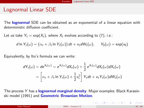
Lognormal Linear SDE
The lognormal SDE can be obtained as an exponential of a linear equation withdeterministic diffusion coefficient.
Let us take Yt = exp(Xt ), where Xt evolves according to (7), i.e.:
d lnYt(ω) = (αt + βt lnYt(ω)) dt + vtdWt(ω), Y0(ω) = exp(x0)
Equivalently, by Ito’s formula we can write:
dYt(ω) = deXt(ω) = eXt(ω)dXt(ω) +1
2eXt(ω)dXt(ω)dXt(ω)
=
[
αt + βt lnYt(ω) +1
2v2t
]
Ytdt + vtYt(ω)dWt(ω)
The process Y has a lognormal marginal density. Major examples: Black Karasin-ski model (1991) and Geometric Brownian Motion.
Paola Mosconi 20541 – Lecture 1-2 43 / 65
Examples Lognormal Linear SDE
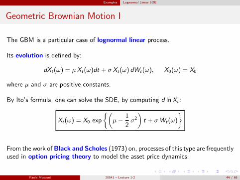
Geometric Brownian Motion I
The GBM is a particular case of lognormal linear process.
Its evolution is defined by:
dXt(ω) = µXt(ω)dt + σ Xt(ω) dWt(ω), X0(ω) = X0
where µ and σ are positive constants.
By Ito’s formula, one can solve the SDE, by computing d lnXt :
Xt(ω) = X0 exp
(
µ− 1
2σ2
)
t + σWt(ω)
From the work of Black and Scholes (1973) on, processes of this type are frequentlyused in option pricing theory to model the asset price dynamics.
Paola Mosconi 20541 – Lecture 1-2 44 / 65
Examples Lognormal Linear SDE
Geometric Brownian Motion II
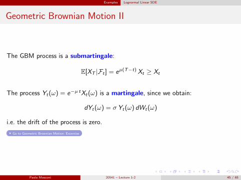
The GBM process is a submartingale:
E[XT |Ft ] = eµ(T−t) Xt ≥ Xt
The process Yt(ω) = e−µ tXt(ω) is a martingale, since we obtain:
dYt(ω) = σ Yt(ω) dWt(ω)
i.e. the drift of the process is zero.
Go to Geometric Brownian Motion: Excercise
Paola Mosconi 20541 – Lecture 1-2 45 / 65
Examples Square Root Process
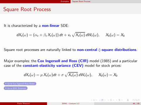
Square Root Process
It is characterized by a non-linear SDE:
dXt(ω) = (αt + βt Xt(ω)) dt + vt√
Xt(ω) dWt(ω), X0(ω) = X0
Square root processes are naturally linked to non-central ξ-square distributions.
Major examples: the Cox Ingersoll and Ross (CIR) model (1985) and a particularcase of the constant-elasticity variance (CEV) model for stock prices:
dXt(ω) = µXt(ω)dt + σ√
Xt(ω) dWt(ω), X0(ω) = X0
Go to Cox Ingersoll Ross Model
Go to SDE: Excercise
Paola Mosconi 20541 – Lecture 1-2 46 / 65
Change of Measure
Outline
1 From Deterministic to Stochastic Differential Equations
2 Ito’s formula
3 Examples
4 Change of Measure
5 No-Arbitrage Pricing
6 Exercises
Paola Mosconi 20541 – Lecture 1-2 47 / 65
Change of Measure
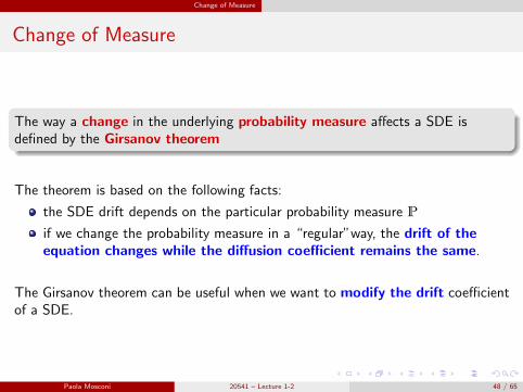
Change of Measure
The way a change in the underlying probability measure affects a SDE isdefined by the Girsanov theorem
The theorem is based on the following facts:
the SDE drift depends on the particular probability measure P
if we change the probability measure in a “regular”way, the drift of theequation changes while the diffusion coefficient remains the same.
The Girsanov theorem can be useful when we want to modify the drift coefficientof a SDE.
Paola Mosconi 20541 – Lecture 1-2 48 / 65

Change of Measure
Radon-Nikodym Derivative
Two measures P∗ and P on the space (Ω,F , (Ft)t) are said to be equivalent, i.e.P∗ ∼ P, if they share the same sets of null probability.
When two measures are equivalent, it is possible to express the first in terms ofthe second through the Radon-Nikodym derivative.
There exists a martingale ρt on (Ω,F , (Ft)t ,P) such that
P∗ =
∫
A
ρt(ω) dP(ω), A ∈ Ft
which can be written as:
dP∗
dP
∣
∣
∣
∣
Ft
= ρt
The process ρt is called the Radon-Nikodym derivative of P∗ with respect to P
restricted to Ft .
Paola Mosconi 20541 – Lecture 1-2 49 / 65
Change of Measure
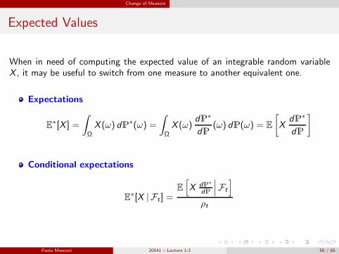
Expected Values
When in need of computing the expected value of an integrable random variableX , it may be useful to switch from one measure to another equivalent one.
Expectations
E∗[X ] =
∫
Ω
X (ω) dP∗(ω) =
∫
Ω
X (ω)dP∗
dP(ω) dP(ω) = E
[
XdP∗
dP
]
Conditional expectations
E∗[X | Ft ] =
E
[
X dP∗
dP
∣
∣
∣Ft
]
ρt
Paola Mosconi 20541 – Lecture 1-2 50 / 65
Change of Measure
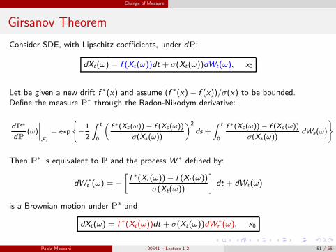
Girsanov Theorem
Consider SDE, with Lipschitz coefficients, under dP:
dXt(ω) = f (Xt(ω))dt + σ(Xt(ω))dWt(ω), x0
Let be given a new drift f ∗(x) and assume (f ∗(x)− f (x))/σ(x) to be bounded.Define the measure P∗ through the Radon-Nikodym derivative:
dP∗
dP(ω)
∣
∣
∣
∣
Ft
= exp
−
1
2
∫ t
0
(
f ∗(Xs (ω)) − f (Xs (ω))
σ(Xs (ω))
)2
ds +
∫ t
0
f ∗(Xs (ω)) − f (Xs (ω))
σ(Xs (ω))dWs(ω)
Then P∗ is equivalent to P and the process W ∗ defined by:
dW ∗t (ω) = −
[
f ∗(Xt(ω))− f (Xt(ω))
σ(Xt(ω))
]
dt + dWt(ω)
is a Brownian motion under P∗ and
dXt(ω) = f ∗(Xt(ω))dt + σ(Xt(ω))dW∗t (ω), x0
Paola Mosconi 20541 – Lecture 1-2 51 / 65
Change of Measure
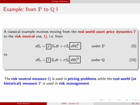
Example: from P to Q I
A classical example involves moving from the real world asset price dynamics Pto the risk neutral one, Q, i.e. from
dSt = µ Stdt + σSt dWPt under P (9)
to
dSt = r Stdt + σSt dWQt under Q (10)
The risk neutral measure Q is used in pricing problems while the real-world (orhistorical) measure P is used in risk management.
Paola Mosconi 20541 – Lecture 1-2 52 / 65
Change of Measure
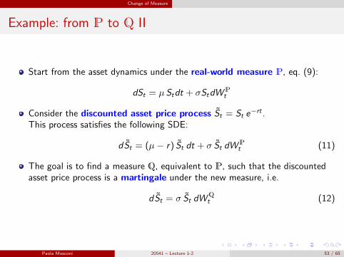
Example: from P to Q II
Start from the asset dynamics under the real-world measure P, eq. (9):
dSt = µ Stdt + σStdWPt
Consider the discounted asset price process St = St e−rt .
This process satisfies the following SDE:
dSt = (µ− r) St dt + σ St dWPt (11)
The goal is to find a measure Q, equivalent to P, such that the discountedasset price process is a martingale under the new measure, i.e.
dSt = σ St dWQt (12)
Paola Mosconi 20541 – Lecture 1-2 53 / 65
Change of Measure
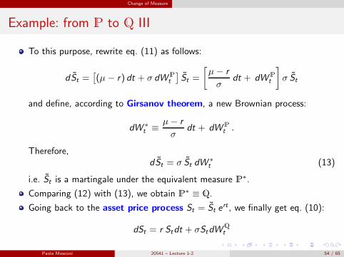
Example: from P to Q III
To this purpose, rewrite eq. (11) as follows:
dSt =[
(µ− r) dt + σ dWPt
]
St =
[
µ− r
σdt + dWP
t
]
σ St
and define, according to Girsanov theorem, a new Brownian process:
dW ∗t ≡ µ− r
σdt + dWP
t .
Therefore,dSt = σ St dW
∗t (13)
i.e. St is a martingale under the equivalent measure P∗.
Comparing (12) with (13), we obtain P∗ ≡ Q.
Going back to the asset price process St = St ert , we finally get eq. (10):
dSt = r Stdt + σStdWQt
Paola Mosconi 20541 – Lecture 1-2 54 / 65
No-Arbitrage Pricing
Outline
1 From Deterministic to Stochastic Differential Equations
2 Ito’s formula
3 Examples
4 Change of Measure
5 No-Arbitrage Pricing
6 Exercises
Paola Mosconi 20541 – Lecture 1-2 55 / 65
No-Arbitrage Pricing
No-Arbitrage Pricing
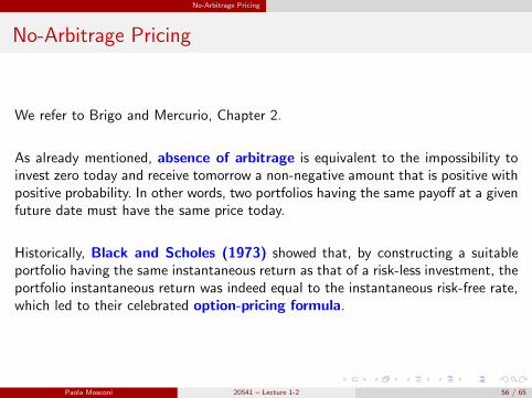
We refer to Brigo and Mercurio, Chapter 2.
As already mentioned, absence of arbitrage is equivalent to the impossibility toinvest zero today and receive tomorrow a non-negative amount that is positive withpositive probability. In other words, two portfolios having the same payoff at a givenfuture date must have the same price today.
Historically, Black and Scholes (1973) showed that, by constructing a suitableportfolio having the same instantaneous return as that of a risk-less investment, theportfolio instantaneous return was indeed equal to the instantaneous risk-free rate,which led to their celebrated option-pricing formula.
Paola Mosconi 20541 – Lecture 1-2 56 / 65
No-Arbitrage Pricing
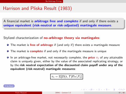
Harrison and Pliska Result (1983)
A financial market is arbitrage free and complete if and only if there exists aunique equivalent (risk-neutral or risk-adjusted) martingale measure.
Stylized characterization of no-arbitrage theory via martingales:
The market is free of arbitrage if (and only if) there exists a martingale measure
The market is complete if and only if the martingale measure is unique
In an arbitrage-free market, not necessarily complete, the price πt of any attainableclaim is uniquely given, either by the value of the associated replicating strategy, orby the risk neutral expectation of the discounted claim payoff under any of theequivalent (risk-neutral) martingale measures:
πt = E[D(t,T )ΠT |Ft ]
Go Back
Paola Mosconi 20541 – Lecture 1-2 57 / 65
Exercises
Outline
1 From Deterministic to Stochastic Differential Equations
2 Ito’s formula
3 Examples
4 Change of Measure
5 No-Arbitrage Pricing
6 Exercises
Paola Mosconi 20541 – Lecture 1-2 58 / 65
Exercises
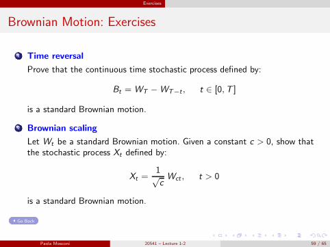
Brownian Motion: Exercises
1 Time reversal
Prove that the continuous time stochastic process defined by:
Bt = WT −WT−t , t ∈ [0,T ]
is a standard Brownian motion.
2 Brownian scaling
Let Wt be a standard Brownian motion. Given a constant c > 0, show thatthe stochastic process Xt defined by:
Xt =1√cWct , t > 0
is a standard Brownian motion.
Go Back
Paola Mosconi 20541 – Lecture 1-2 59 / 65
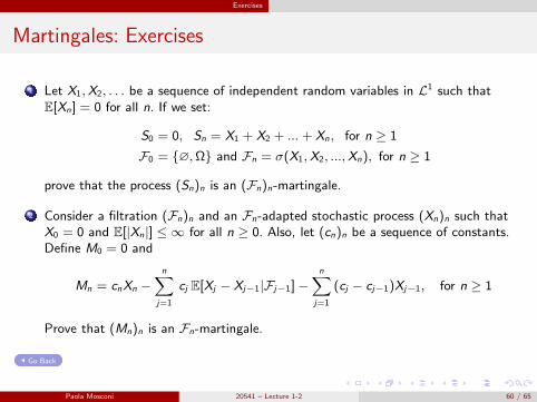
Exercises
Martingales: Exercises
1 Let X1,X2, . . . be a sequence of independent random variables in L1 such thatE[Xn] = 0 for all n. If we set:
S0 = 0, Sn = X1 + X2 + ... + Xn, for n ≥ 1
F0 = ∅,Ω and Fn = σ(X1,X2, ...,Xn), for n ≥ 1
prove that the process (Sn)n is an (Fn)n-martingale.
2 Consider a filtration (Fn)n and an Fn-adapted stochastic process (Xn)n such thatX0 = 0 and E[|Xn|] ≤ ∞ for all n ≥ 0. Also, let (cn)n be a sequence of constants.Define M0 = 0 and
Mn = cnXn −n
∑
j=1
cj E[Xj − Xj−1|Fj−1]−n
∑
j=1
(cj − cj−1)Xj−1, for n ≥ 1
Prove that (Mn)n is an Fn-martingale.
Go Back
Paola Mosconi 20541 – Lecture 1-2 60 / 65

Exercises
Ito’s formula: Exercises
1 Consider a standard one-dimensional Brownian motion Wt . Use Ito’s formula tocalculate:
W 2t = t + 2
∫ t
0
WsdWs
and
W 27t = 351
∫ t
0
W 25s ds + 27
∫ t
0
W 26s dWs
2 Consider a standard one-dimensional Brownian motion Wt . Given k ≥ 2 and t ≥ 0,use Ito’s formula to prove that:
E[W kt ] =
1
2k(k − 1)
∫ t
0
E[W k−2u ]du
Use this expression to calculate E[W 4t ] and E[W 6
t ].
Hint: stochastic integrals are martingales, so their expectation is zero.
Go Back
Paola Mosconi 20541 – Lecture 1-2 61 / 65
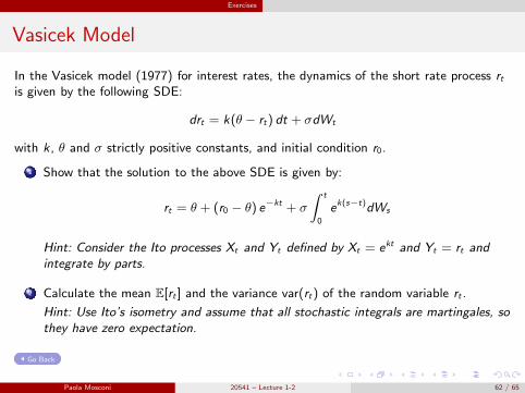
Exercises
Vasicek Model
In the Vasicek model (1977) for interest rates, the dynamics of the short rate process rtis given by the following SDE:
drt = k(θ − rt) dt + σdWt
with k , θ and σ strictly positive constants, and initial condition r0.
1 Show that the solution to the above SDE is given by:
rt = θ + (r0 − θ) e−kt + σ
∫ t
0
ek(s−t)dWs
Hint: Consider the Ito processes Xt and Yt defined by Xt = ekt and Yt = rt andintegrate by parts.
2 Calculate the mean E[rt ] and the variance var(rt) of the random variable rt .
Hint: Use Ito’s isometry and assume that all stochastic integrals are martingales, sothey have zero expectation.
Go Back
Paola Mosconi 20541 – Lecture 1-2 62 / 65
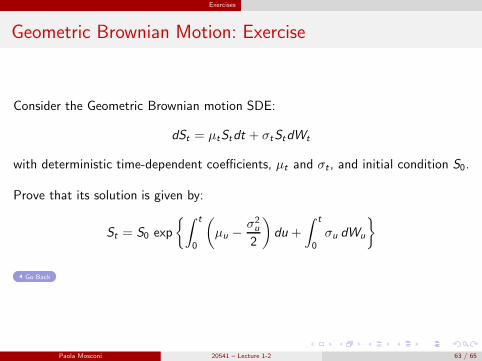
Exercises
Geometric Brownian Motion: Exercise
Consider the Geometric Brownian motion SDE:
dSt = µtStdt + σtStdWt
with deterministic time-dependent coefficients, µt and σt , and initial condition S0.
Prove that its solution is given by:
St = S0 exp
∫ t
0
(
µu −σ2u
2
)
du +
∫ t
0
σu dWu
Go Back
Paola Mosconi 20541 – Lecture 1-2 63 / 65
Exercises
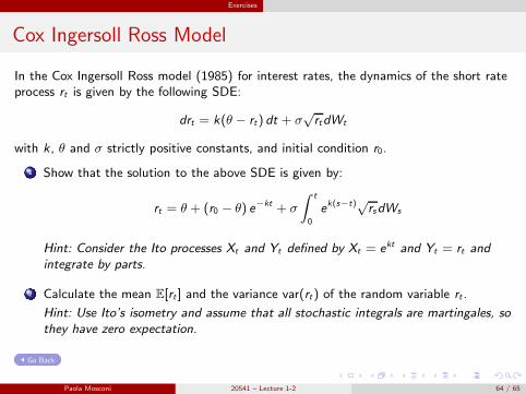
Cox Ingersoll Ross Model
In the Cox Ingersoll Ross model (1985) for interest rates, the dynamics of the short rateprocess rt is given by the following SDE:
drt = k(θ − rt) dt + σ√rtdWt
with k , θ and σ strictly positive constants, and initial condition r0.
1 Show that the solution to the above SDE is given by:
rt = θ + (r0 − θ) e−kt + σ
∫ t
0
ek(s−t)√rsdWs
Hint: Consider the Ito processes Xt and Yt defined by Xt = ekt and Yt = rt andintegrate by parts.
2 Calculate the mean E[rt ] and the variance var(rt) of the random variable rt .
Hint: Use Ito’s isometry and assume that all stochastic integrals are martingales, sothey have zero expectation.
Go Back
Paola Mosconi 20541 – Lecture 1-2 64 / 65
Exercises
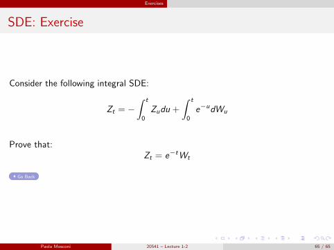
SDE: Exercise
Consider the following integral SDE:
Zt = −∫ t
0
Zudu +
∫ t
0
e−udWu
Prove that:Zt = e−tWt
Go Back
Paola Mosconi 20541 – Lecture 1-2 65 / 65