Embed Size (px)
Citation preview
Influence of Saturation and Geometry on Surface Electrical
Resistivity Measurements
Jose Miguel Sanchez Marquez
A Thesis
in
The Department
of
Building, Civil and Environmental Engineering
Presented in Partial Fulfillment of the Requirements
for the Degree of Master of Applied Science Building Engineering at
Concordia University
Montreal, Quebec, Canada
June 2015
© Jose Miguel Sanchez Marquez, 2015
CONCORDIA UNIVERSITY
School of Graduate Studies
This is to certify that the thesis prepared
By: Jose Miguel Sanchez Marquez
Entitled: Influence of Saturation and Geometry on Surface Electrical Resistivity
Measurements
and submitted in partial fulfillment of the requirements for the degree of.
Master of Applied Science (Building Engineering)
complies with the regulations of the University and meets the accepted standards with
respect to originality and quality.
Signed by the final Examining Committee:
Dr. Christopher W. Trueman Chair
Dr. Fuzhan Nasiri Examiner
Dr. Luis Amador Examiner
Dr. Michelle R. Nokken Supervisor
Approved by
Chair of Department or Graduate Program Director
June 2015
Dean of Faculty
Abstract
Influence of Saturation and Geometry on Surface Electrical Resistivity
Measurements
Jose Miguel Sanchez Marquez
Concordia University, 2015
Non-destructive tests are the future for early concrete deterioration detection. The
interest in surface electrical resistivity as for the quality control of concrete structures has
increased in the last several years. A standardized laboratory method has recently been
adopted as AASHTO TP 95-11 and an ASTM method is under consideration. Both these
methods measure surface resistance by a Wenner four-electrode probe device, in which the
electrodes are equally spaced on the surface of saturated concrete elements. Currently, the
standardized method is restricted to laboratory specimens. For this method to be applicable
to field measurements requires first to identify how much time a concrete element needs to
reach saturation and how reliable resistivity values are under different saturation stages.
Phase one of this research investigated the duration of saturation required to achieve stable
resistivity for 20 mixture designs at a range of ages. It was generally determined that
resistivity varies until 24 hours. Past that duration, some increases in surface resistivity
were observed and attributed to further hydration. In the field, concrete elements are
generally large and the assumptions of infinite geometry hold. Lab specimens, on the other
hand, have a constricted flow of electrical current. In Phase two, the influences of geometry
and saturation fluid were examined. It was found that using published geometrical
conversion factors did not result in equivalent surface resistivity between cylinders and
small slabs or for cylinders of different sizes, suggesting more work required in this area.
The use of tap water was investigated as it would be more available on site; it was found
that at 28 days, there were minimal differences between tap water and limewater. At later
ages, limewater generally resulted in higher resistivity. Phase Three investigated published
temperature corrections to adjust site measured resistivity to standard temperature.
Regardless of the correction, significant difference was observed between the site and
laboratory measurements. Lastly in Phase four, two alternate techniques were tested for
potential on site use. It was found that neither resulted in any significant changes in
resistivity.
iv
Acknowledgement
It is with sincere and with enormous gratitude that I thank my advisor Dr. Michelle R.
Nokken for choosing me and believe in me. This experience was a dream come true. She
never doubted my abilities and always motivated me with her knowledge, kindness and
patience. Thanks again Professor for your supervision, consideration and your strong
commitment in this work
v
Dedication
To the greatest of my life, mom, dad and Andres;
Thanks for the company, patience, positive energy and trust through the distance, without your
support this work never could have been done. You are always in my mind, los amo.
vi
Table of Contents
Abstract ............................................................................................................................... ii
1 Introduction ................................................................................................................. 1
1.1 Research Objectives ............................................................................................. 4
1.2 Chapter Outline .................................................................................................... 5
1.3 List of Abbreviations ............................................................................................ 7
2 Literature Review ........................................................................................................ 8
2.1 Terminology ......................................................................................................... 9
2.1.1 Porosity ....................................................................................................... 10
2.1.2 Permeability ................................................................................................ 10
2.1.3 Sorptivity..................................................................................................... 10
2.1.4 Distinguishing between permeability and porosity..................................... 11
2.2 Electrical Methods for Concrete Durability ....................................................... 14
2.2.1 Background ................................................................................................. 15
2.2.2 Electrical Conductivity Tests ...................................................................... 20
2.2.3 Electrical Resistivity Tests .......................................................................... 23
2.3 Factors Influencing Probe Spacing in the Wenner Four Probe Technique ........ 34
2.3.1 Surface Contacts ......................................................................................... 34
2.3.2 Geometrical Constraints.............................................................................. 35
2.3.3 Probe Spacing ............................................................................................. 38
2.3.4 Specimen Geometry .................................................................................... 39
2.4 General Factors Influencing Electrical Resistivity due to Concrete Mixture .... 43
2.4.1 Effects of Water Cement Ratio Effect on Surface Resistivity .................... 43
2.4.2 Pore Solution in Cementitious Systems ...................................................... 44
2.4.3 Supplementary Cementitious Materials ...................................................... 46
2.4.4 Concrete Age .............................................................................................. 49
2.4.5 Presence of Steel Reinforcing Bars ............................................................. 51
2.4.6 Effect of Surface Layer of Different Resistivity ......................................... 55
2.4.7 Concrete Non – Homogeneity .................................................................... 56
2.5 General Factors Influencing Electrical Resistivity due to External Environment
56
vii
2.5.1 Rainfall ........................................................................................................ 57
2.5.2 Moisture Content and Temperature ............................................................ 57
2.5.3 Saturation Degree (SD) ............................................................................... 64
3 Laboratory and Work Practice Methodology ............................................................ 67
3.1 Phase One – Influence of Saturation Duration ................................................... 68
3.2 Phase Two – Influence of Samples Storage under Different Solutions and
Specimen Geometry ...................................................................................................... 71
3.2.1 City of Montreal (Ville de Montréal) Samples ........................................... 73
3.3 Phase Three – Analysis of Correlations to Normalize Temperature Effect on Site
and the Influence of Curved and Plane Surfaces ........................................................... 74
3.4 Phase Four – Influence of Saturation Methods Techniques ............................... 78
3.4.1 Water Pressure Saturation ........................................................................... 80
3.4.2 Ponding Saturation ...................................................................................... 80
4 Results of Phases ....................................................................................................... 82
4.1 Phase One - Influence of Saturation Degree ...................................................... 82
4.1.1 Influence of Saturation 28 Days ................................................................. 83
4.1.2 Influence of Saturation – 56 Days .............................................................. 87
4.1.3 Influence of Saturation – 91 days ............................................................... 92
4.1.4 Influence of Concrete Age and Supplementary Materials (SCMs) on
Surface Electrical Resistivity..................................................................................... 95
4.2 Phase Two – Influence of Samples Storage under Different Solutions and
Specimen Geometry .................................................................................................... 109
4.2.1 Specimen Geometry .................................................................................. 110
4.2.2 Sample Storage under Different Solutions ............................................... 117
4.3 Phase Three – Analysis of Correlations to Normalize Temperature Effect on Site
and the Influence of Curved and Plane Surfaces ......................................................... 123
4.3.1 Evaluation of Correlations to Normalize Temperature Effects ................ 123
4.3.2 Differences between Curved and Plane Surfaces ..................................... 125
4.4 Phase Four - Influence of Saturation Methods Techniques ............................. 129
4.4.1 Water Pressure Saturation ......................................................................... 129
4.4.2 Ponding Saturation .................................................................................... 133
5 Discussion ................................................................................................................ 139
5.1 Minimum Duration Time to Achieve Reliable Surface Resistivity Values ..... 140
5.1.1 Differences on Resistivity values in Standard Cylinders Ø10x20cm ....... 140
viii
5.1.2 Differences on Resistivity values in Circular Slabs Ø30x12cm ............... 143
5.2 The Geometry Effect on Surface Resistivity.................................................... 144
5.3 Misreading Surface Electrical Resistivity Results due to Poor Saturation and
Temperature and Moisture Effect ............................................................................... 147
6 Conclusions ............................................................................................................. 150
7 Recommendations ................................................................................................... 153
References ....................................................................................................................... 156
ix
Table of Figures
Figure 1. Types of porous media from Baker 1985. ...................................................................... 11
Figure 2. Porosity and permeability modular relationship from (Heubeck, C. et al., 2004). ......... 12
Figure 3. Hardening procedure evolution for cement paste from Powers et al., 1960. .................. 13
Figure 4. Pore network examples: a) connected pore network; b) not connected pore network by
Neville et al. (1987). ................................................................................................................. 17
Figure 5. ASTM C1202-07 rapid chloride permeability test ......................................................... 21
Figure 6. Surface resistivity device after Proceq SA manual (2013). ............................................ 24
Figure 7. Bulk Resistivity setup after Shahroodi, (2010)............................................................... 25
Figure 8. Covercrete layer composition (drawing without scale). ................................................. 27
Figure 9. Setup of Surface disc test after Polder et al., (2000). ..................................................... 28
Figure 10. Setup of surface four square – probe array test after Lataste (2003). ........................... 28
Figure 11. Embedded electrodes after McCarter et al., 2009 ......................................................... 30
Figure 12. Schematic representation of four-electrode resistivity test by Kessler al. (2008). ....... 31
Figure 13. Correlation between Rapid Chloride Permeability and Surface Resistivity on saturated
samples at 28 days reproduced from Kessler et al., 2008. ........................................................ 32
Figure 14. Representation of resistivity measurements of concrete samples from Chun-Tao et al.
(2014). ....................................................................................................................................... 35
Figure 15. Relationship between the correction geometry factor (k) and standard cylinders
(10x20cm) adapted from Morris et al. (1996). ......................................................................... 37
Figure 16. Probe spacing effect on the penetration depth using the four-line Wenner probe device
reproduced from Polder (2001). ................................................................................................ 39
Figure 17. Conductivity in porous material, a) ions released in the pore solution; b) porosity; c)
connectivity, reproduced from Spragg et al. (2013). ................................................................ 45
x
Figure 18. Scanning electron microscope of fly ash particles by Belviso et al., (2011). ............... 47
Figure 19. Scanning electron microscope of Slag particles by Rađenović et al. (2013). ............... 48
Figure 20. Effect of the age in concrete samples after Kessler et al., (2008). ....................... 50
Figure 21. Measurement locations with one rebar, probe spacing of 3cm (left) and 5cm (right)
(Presuel-Moreno et al., 2010). .................................................................................................. 53
Figure 22. Measurement locations with four rebar, probe spacing of 3cm (above), 5 cm (bellow)
by Presuel - Moreno et al., (2010). ........................................................................................... 55
Figure 23. Moisture degree (MD) effect on surface resistivity after Larsen et al., (2007a). ........ 59
Figure 24.Temperature effect on surface resistivity after Larsen et al., (2007a). .......................... 60
Figure 25. Ponding saturation examples a) Wenner-four probe ; b) Closed view of Wenner
device; c) GPM device; d) Unreliable resistivity values, from Strategic Highway Research
Program SHRP2, < http://www.ndtoolbox.org/content/bridge/er-description> ....................... 66
Figure 26. Marks for the four line electrodes locations. ................................................................ 70
Figure 27. Geometry samples (a) standard cylinder (10x20cm) (b) circular slab (Ø 30x12cm)
(Drawings without scale). ......................................................................................................... 72
Figure 28. Sidewalks location at North - East of Montreal, QC. CA. ........................................... 75
Figure 29. Sidewalks street location - Av. Poutrincourt between Av. Louis Danton and rue Viel,
Montreal, QC.CA. ..................................................................................................................... 76
Figure 30. Sidewalks street view; a) VdeMTL10PV; b) VdeMTL Temoin or (formule 3VM-10)
and c - d) VdeMTL25PV .......................................................................................................... 77
Figure 31. Circular slabs geometry Ø30x12cm (Drawings without scale). ................................... 79
Figure 32. Ponding saturation simulation on ø30x12cm samples. ................................................. 81
Figure 33. Resistivity Values against Saturation Time Mixture 100TI (28 days). ........................ 83
Figure 34. Resistivity Values against Saturation Time Mixture 50L–50S (28 days). ................... 84
Figure 35. Resistivity Values against Saturation Time Mix 50TI-50S (28 days). ......................... 85
Figure 36. Resistivity Values against Saturation Time Mix 50TI-30FA-20S (28 days). ............... 85
xi
Figure 37. Resistivity Values against Saturation Time Mix 50TI-20FA-30S (28 days). ............... 86
Figure 38. Resistivity Values against Saturation Time Mix 100TI (56 days)................................ 88
Figure 39. Resistivity Values against Saturation Time Mix 50L-50S (56 days). .......................... 89
Figure 40. Resistivity Values against Saturation Time Mix 50TI-50S (56 days). ......................... 90
Figure 41. Resistivity values against Saturation Time Mix 50TI-20FA-30S (56 days). ............... 91
Figure 42. Resistivity values against Saturation Time Mix 50TI-30FA-20S (56 days). ............... 91
Figure 43. Resistivity Values against Saturation Time Mix 100TI (91 days)................................ 93
Figure 44. Resistivity Values against Saturation Time Mixture 50TI-50S (91 days). ................... 94
Figure 45. Resistivity Values against Saturation Time Mixture 50TI-20FA-30S (91 days). ........ 94
Figure 46. Resistivity increase over time for mixtures with w/c close to 0.50. ............................. 98
Figure 47. Resistivity variation through three periods of time – Mix 100TI. ................................ 99
Figure 48. Resistivity variation through three periods of time – Mix 75TI – 25FA. ................... 100
Figure 49. Resistivity Values for Mix 100TI within a range of w/c at different ages. ................ 101
Figure 51. Resistivity Values for Mix 50TI-20FA-30S within a range of w/c at different ages. 102
Figure 50. Resistivity Values for Mix 50TI-50S within a range of w/c at different ages. ........... 102
Figure 52. Relationship between water absorption and surface resistivity at 91 Days. ............... 104
Figure 53. Screenshot of the web application developed by Bentz (2007). ................................. 106
Figure 54. Estimated pore solution conductivity and surface resistivity comparison at 91 days. 108
Figure 55. Standard cylinders Ø10x20cm and circular slab Ø30x12cm...................................... 109
Figure 56. Effect of geometry factor before and after correction on mixtures 100TI with w/c equal
to 0.40 and 0.50 at 28 days. .................................................................................................... 111
Figure 57. Effect of geometry factor Correction for City of Montreal samples. ......................... 114
Figure 58. Resistivity values within the first hour – Mature Mixtures. Sept 2013. ..................... 117
Figure 59. Resistivity values up to 72 hours – Mature Mixtures. Sept 2013. .............................. 118
Figure 60. Resistivity values within the first hour – Mature Mixtures. Feb. 2014. ..................... 119
Figure 61. Resistivity values up to 72 hours – Mature Mixtures. Feb. 2014. .............................. 120
xii
Figure 62. Wenner four probe pattern location over concrete sidewalk ...................................... 123
Figure 63. Differences between temperatures on mixtures samples. ........................................... 124
Figure 64. Differences between plane and curved surfaces mixture VdeMTL TEMOIN. .......... 126
Figure 65. Differences between plane and curved surfaces mixture VdeMTL 10PV. ................ 127
Figure 66. Differences between plane and curved surfaces mixture VdeMTL 25PV .............. 127
Figure 67. Water pressure saturation results mixture 100TI w/c 0.40 ......................................... 129
Figure 69. Water pressure saturation results mixture 50TI 30FA20S w/c 0.40 ........................... 130
Figure 68. Water pressure saturation results mixture 100TI w/c 0.50 ......................................... 130
Figure 70. Comparison between immerse and pressurized water Mix -100TI w/c 0.40 ............. 131
Figure 71. Comparison between immerse and pressurized water Mix - 100TI w/c 0.50 ............ 131
Figure 72. Comparison between immersed and pressurized water Mix- 50TI30FA20S w/c
0.40 ......................................................................................................................................... 132
Figure 73. Ponding saturation Mix - 100TI w/c 0.40 ................................................................... 134
Figure 74. Ponding saturation Mix- 100TI w/c 0.50 .................................................................... 134
Figure 75. Ponding saturation Mix- 50TI30FA20S w/c 0.40. ..................................................... 135
Figure 76. Differences through time in surface resistivity Mix - 100TI w/c 0.40. ...................... 136
Figure 77. Differences through time in surface resistivity Mix -100TI w/c 0.50. ....................... 137
Figure 78. Differences through time in surface resistivity Mix -
50TI30FA20S w/c 0.40........................................................................................................... 138
Figure 79. Resistivity Values on Mixes with w/c close to 0.40 (28 days). .................................. 141
Figure 80. Geometry relation Phase Two – All mixtures ............................................................ 146
Figure 81. Geometry relation Phase Two – Portland mixtures .................................................... 146
xiii
Table of Tables
Table 1. Time required for achieving a discontinuous pore system Powers et al., 1959. .............. 14
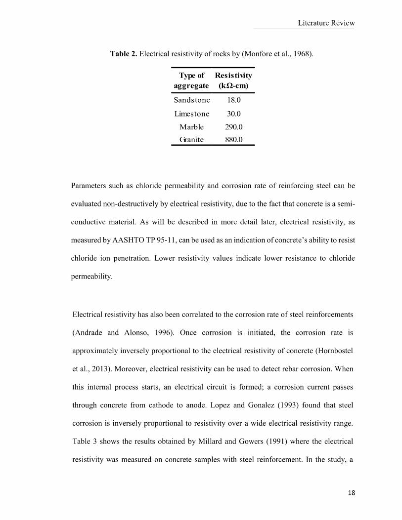
Table 2. Electrical resistivity of rocks by (Monfore et al., 1968). ................................................. 18
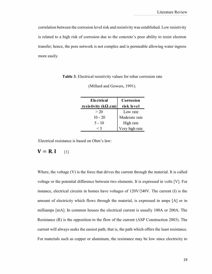
Table 3. Electrical resistivity values for rebar corrosion rate (Millard and Gowers, 1991). .......... 19
Table 4. Chloride ion penetrability based on charge passed (ASTM C1202, 2007). ..................... 22
Table 5. Correlation between electrical resistivity and chloride ion penetration AASHTO, TP 95-
11 (2011) reproduced from Yanbo, L. et al. (2014). ................................................................. 33
Table 6. Laboratory Mixtures after Shahroodi (2010). ................................................................. 38
Table 7. Corrected resistivity of cylinders and slabs (Bryant et al. 2009). .................................... 40
Table 8. Corrected resistivity of cylinders and slabs (Shahroodi 2010). ....................................... 41
Table 9. Mixtures design by Rupnow et al., (2011). ...................................................................... 44
Table 10. Resistivity of the Laboratory Mixes after Kessler et al. (2008). .................................... 49
Table 11. Resistivity values with one rebar by Presuel - Moreno et al., (2010). ........................... 53
Table 12. Resistivity values with four rebar by Presuel-Moreno et al., (2010). ............................ 54
Table 13. Type of cement and admixtures used by Liu et al., (2014). ........................................... 62
Table 14. Equations according to mixture properties by Liu et al., (2014). .................................. 63
Table 15. Phase One Mixture Designs and Properties. .................................................................. 69
Table 16. Concrete mixtures by city of Montreal .......................................................................... 74
Table 17. Surface resistivity through time (days) for standard cylinders (ø10x20cm). ................. 96
Table 18. Pore solution conductivity and surface resistivity at 91 days. ..................................... 107
Table 19. Average surface resistivity values for Phase Two mixtures ........................................ 110
Table 20. Percentage differences before and after apply the geometry correction factor. ........... 112
Table 21. Average differences on specimen geometry from City of Montreal............................ 115
xiv
Table 22. Average electrical resistivity and percentage differences between top and bottom layers
from circular slabs. ................................................................................................................. 116
Table 23. Influence of storage and specimen geometry on electrical surface resistivity. ............ 121
Table 24. Average Percentage Differences between Lime Water (LW) and Tap Water (TW) After
48 Hours Immersion. .............................................................................................................. 122
Table 25. Percent Differences through Saturation Time – Ø10x20cm samples. ......................... 142
Table 26. Percent Differences through Saturation Time – Ø30x12cm samples. ......................... 144
Table 27. Electrical resistivity values for rebar corrosion rate and AASHTO, TP 95-11 (2011) 148
Table 28. Correlation between electrical resistivity and chloride ion penetration. ...................... 149
1
1 Introduction
Concrete is one of the most commonly used products today in the construction industry.
This product needs to be mixed, transported, placed, finished and cured to exhibit the
desired performance. Once placed, finished and cured, two main properties that take
special attention are compressive strength and durability. The first is the ability of concrete
to resist mechanical stresses and the second one can be defined as, the concrete’s ability
to keep quality, form and serviceability under different environmental conditions over a
period of time without requiring excessive effort for maintenance. Durability is mainly
influenced by: (a) hardened concrete properties, (b) environmental exposure conditions
and (c) construction practices.
Hardened concrete properties are a function of the water to cementitious material ratio and
mixture design. Particularly important for durability are the cement paste’s pore size and
distribution. For the case of high performance concrete (HPC), the pore structure should
be as impervious as possible (Swamy 1996). This will prevent the degradation process due
to environmental conditions that involves the penetration and subsequent movement of
air, water or other fluids transporting aggressive agents into the concrete pore system.
These conditions can generate deterioration due to freezing and thawing, sulfate attack,
alkali-silica and alkali-carbonate reactions (Bryant et al. 2009) or corrosion of reinforcing
steel. Reinforcement corrosion is one of the most prevalent forms of deterioration, and
Introduction
2
once corrosion has initiated, cracks in concrete can propagate (Presuel-Moreno et al.
2010).
Construction practices also greatly influence concrete’s durability due to the human factor
involved. The correct placement, consolidation, finishing and curing processes are steps
that can lead to the achievement of the required pore network and maximum density. One
of the most common construction practices issues is failure in proper consolidating and
placing concrete, which can result in honeycombing. Also, it can be found as a result of
excessive vibration, segregation and air-void system alteration which can lead to reducing
the concrete’s resistance of freezing and thawing (Taylor et al., 2013). In other words, a
good durable concrete will be attained if the concrete has a low water to cement ratio, has
achieved adequate thermal and moisture curing, and has achieved a discontinuous
capillary pore structure free of significant micro or macro defects.
Consequently, the penetration properties, such as resistance to absorption and permeation,
should be used as the principal criteria for determining concrete’s durability. Since the
permeability of the outer zone of concrete can be very different from that of the bulk
concrete due to compaction, bleeding, finishing and curing, as well as the choice of
constituent materials used, the solution to the problem of durability in structures is most
likely to come about from understanding of its outer layer or covercrete. (DeSouza 1996).
Introduction
3
Currently there is no standardized, non-destructive technique or method to measure in-
place concrete durability. Several methods exist for laboratory investigations, but many
are time consuming. Electrically based methods have been identified as having the
potential to be rapid tests for durability (Polder, 2005). One potential method is AASHTO
TP 95-11. Presently, it is only standardized as a laboratory method, but the fact is that it
is portable and is therefore relevant for in-situ investigation. This method utilizes a Wenner
probe with four equally spaced electrodes. In the Wenner four electrode technique, an
alternating current is applied between the outer two electrodes and the voltage is measured
between the middle two electrodes indicating the electrical surface resistivity of the
element. A lower electrical resistivity value is obtained when the applied electrical current
can easily pass through the pore structure, which in terms of permeability corresponds to
a highly permeable concrete (Shahroodi 2010).
Since only the surface is being tested, this procedure has the advantage of measuring
concrete’s quality and the influence of alternative curing methods on the exposed surface.
It should be mentioned that several factors can influence concrete’s surface resistivity such
as inclusion of supplementary cementitious materials, saturation degree, temperature,
water to cement ratio (w/c) and age. These factors will be further detailed in the Literature
review chapter.
Introduction
4
1.1 Research Objectives
The primary focus of this study is to analyze the use of the electrical resistivity device as a
suitable, non-destructive method to evaluate the potential durability of the surface layer or
covercrete in field situations. Since moisture content of concrete in the field will vary, a
large part of the research was devoted to quantify the influence of surface saturation on the
test, comparing results obtained from full immersion, humid air, pressurized water and
static surface ponding with a Wenner four probe with four equally spaced electrodes was
used from the commercial brand Proceq that works with frequency of 40Hz. The specific
objectives are to:
Determine the immersion time required for concrete to achieve a stable resistivity
in the laboratory. Determine the influence of water cement ratio (w/c),
supplementary cementitious materials and concrete age on the saturation required
for stable surface electrical resistivity test.
Examine how the specimen’s geometry (cylinders, circular slabs, field placed
concrete) influences the surface electrical resistivity after periods of saturation.
Determine if the use of tap water may be feasible for saturation purposes.
Investigate alternate methods to saturate concrete elements to obtain reliable
surface electrical measurements but in less time, similar to the ones obtained in the
laboratory after long periods of saturation.
Introduction
5
1.2 Chapter Outline
The thesis begins with a literature review about the importance of electrical resistivity
methods and how they are related to the concrete’s physical properties such as, porosity
and permeability. In addition, the background of different types of electrical methods
developed through the years bearing on concrete’s quality assurance is considered with
special emphasis on the Wenner four-electrode technique. Outlined are some of the
common mistakes that can be made assessing concrete resistivity plus some steps that can
be taken to minimize errors. In-depth descriptions of the principal factors that influence
surface electrical resistivity such as pore structure, temperature, saturation degree and use
of supplementary cementitious materials are presented.
Chapter 3 details the experimental methodology used to achieve the research objectives
described previously. Several different phases comprise this effort. A commercial device,
based on the Wenner probe device, was primarily used during this research.
Chapter 4 analyses the results from each phase of the experimental program. A detailed
description of how resistivity is influenced by different durations of saturation at different
ages (28, 56 and 91 days) on a total of five binder combinations on cylinders (Ø10x20 cm)
cast under laboratory conditions, establishing the time required for concrete to achieve a
stable resistivity under these conditions as well as analyzing the effect of supplementary
Introduction
6
cementitious materials – blast furnace slag and fly ash on concrete. A second round of
samples were cast using different specimen geometries, circular slabs Ø30x12cm and
standard cylinders Ø10x20cm and Ø15x30cm to analyze the influence of geometry and
surface layer on electrical resistivity. Additionally, both geometry samples were stored
under two solutions to determine if exist different between the surface resistivity measured
values. An analysis is presented further of correlations established to normalize the
temperature effect on site and the influence of curved and plane surfaces are also analyzed.
Lastly, the influence of two different saturation practices on surface electrical resistivity
are presented.
Chapter 5 discusses three main topics; (a) the minimum duration to obtain reliable surface
resistivity values on laboratory samples; (b) Geometry effect and type of solution to
storage; (c) misreading surface electrical resistivity results due to poor saturation based on
results achieved in chapter 4.
Finally, a number of conclusions over this work are presented with recommendations for
future work and suggestions to continue improving a methodology able to achieve reliable
measurements on site situations.
Introduction
7
1.3 List of Abbreviations
ASTM American Society for Testing Materials.
AASHTO American Association of State Highway and Transportation Officials.
W/C Water cement ratio.
ASR Alkali-silica reaction.
HPC High performance concrete.
SCMs Supplementary cementitious materials.
(ɸ) Porosity.
(k) Permeability.
AC Alternating current.
DC Direct current.
(ρ) Resistivity.
(a) Probe spacing.
RCP Rapid Chloride Permeability.
SD Saturation degree.
LW Limewater solution.
TW Tap water.
PC Portland cement type I/II.
TI Mixture with Portland cement type I/II.
FA Fly ash.
S Slag cement.
L Limestone cement.
8
2 Literature Review
Concrete mixture design must be carefully considered in regards to its eventual exposure
conditions. Freezing and thawing, alkali silica reaction and corrosion are the most
commonly encountered deterioration mechanisms. Each of these can be directly related
to the concrete’s pore structure.
Water can enter the pore system and subsequently freeze upon exposure to cold conditions.
The effect of freezing-and-thawing is widely known, in most of the cases it generates deep
and widespread deterioration, especially in permeable concretes (high w/c) more
susceptible to absorb and retain moisture through time. Once, water freezes, it produces
hydraulic pressures in the capillaries and pores of the cement paste and aggregates. If these
pressures exceed the tensile strength of the surrounding paste or aggregate, cracks will
form. Initially, this deterioration will not affect the structural capacity of the element but
will affect the concrete’s durability. Its extent cannot be determined through visual
inspections alone and once it has spread in a large area, it can lead to cracking, scaling,
delamination or spalling (Montgomery et al., 2013). However, in order to improve the
long-term performance, the concrete must have a good air-void system especially in places
with marine environments or with possibility of exposure to deicing salts during winter
seasons in northern countries (Taylor et al., 2013).
Literature Review
9
To minimize the likelihood of alkali-silica reaction (ASR), the use of non-reactive
aggregate, low alkali cement or the use of supplementary cementitious materials is
recommended. These material choices coupled with a discontinuous pore network
minimize the likelihood of deterioration. For reinforced concrete to avoid excessive
carbonation and consequent danger of steel corrosion, the steel should have an adequate
cover of concrete with low permeability. In order resist the effects of sulfate attack,
corrosion and chloride permeability, low permeability for high performance concretes is
highly required.
A durable concrete must have a complex pore network structure, with narrower void
spaces avoiding connectedness between them. Ideally, high performance concretes (HPC)
must have low porosity (ɸ) and low permeability (k) characteristics that are going to be
presented in this section.
2.1 Terminology
Durability of cementitious materials highly depends on their ability to prevent the ingress
of water and deleterious materials (such as chloride ions from de-icing salts) into the
material body. In this section, terms such as, porosity, permeability, and sorptivity will be
described, with special emphasis in the difference between porosity and permeability.
Literature Review
10
2.1.1 Porosity
Porosity is defined as the percentage of void spaces as compared to the total material
volume, in this case, concrete. However, void spaces or pore sizes can easily change over
time due to the continuous hydration and sometimes the deterioration process during the
lifetime of concrete. These pores influence concrete properties as durability, creep,
permeability and shrinkage.
2.1.2 Permeability
Permeability is a property that measures the ability of a fluid to pass through the connected
pathways of a saturated porous material under a pressure gradient. Basically, a material
with high numbers of pore pathways or corridors in its pore network will be more
permeable due to the low resistance to fluid flow under the pressure gradient. As a result,
permeability is linked to durability since it determines the penetration of deleterious
substances into the concrete body that can lead, for example, to corrosion in cases of
reinforced concrete.
2.1.3 Sorptivity
Sorptivity can be described as the tendency of a porous medium to transmit a fluid only by
capillary action without any pressure gradient. When a fluid makes contact with a dry
porous material (e.g. concrete), moisture absorption by capillarity is going to take action.
Literature Review
11
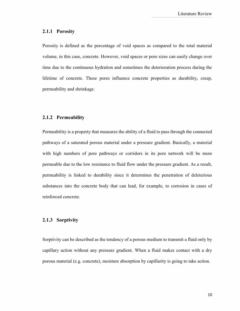
2.1.4 Distinguishing between permeability and porosity
There is neither a direct nor inverse relationship between porosity and permeability. Figure
1 gives four very different examples: (a) shows an impermeable porous rock (e.g. shale);
(b) a porous permeable rock; (c) a rock with very high porosity, but low permeability (e.g.
pumice and clay) and (d) shows a low porosity but highly permeable rock (Baker. 1985).
From Figure 1, it is possible to identify that a pore network can become permeable if there
is continuity and connectedness in the pores or void spaces. In addition, the pore size and
width greatly influence the required pressure and resulting flow rate. The narrower the void
spaces, the higher the pressure must be to force a fluid through the material. For durable
concretes, the rate must be at the lowest possible level to prevent the possibility for intruded
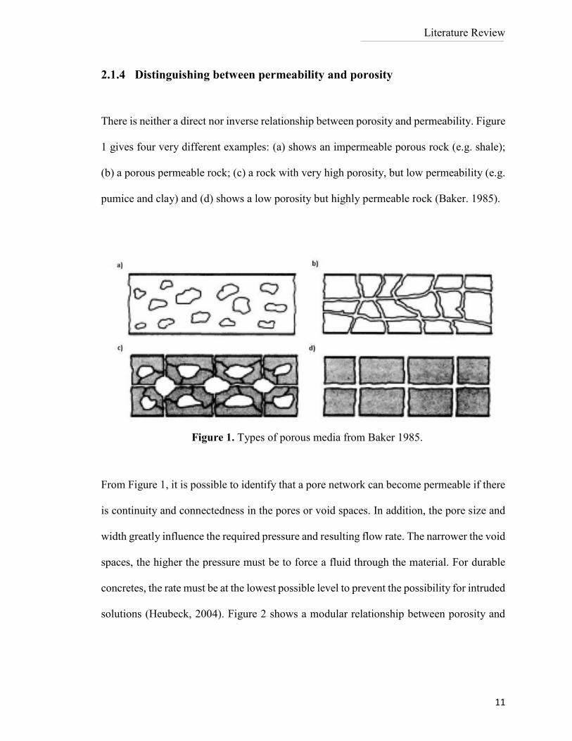
solutions (Heubeck, 2004). Figure 2 shows a modular relationship between porosity and
Figure 1. Types of porous media from Baker 1985.
Literature Review
12
permeability (pore-tube model). Ideally, high performance concretes must have low
porosity (ɸ) and low permeability (k) characteristics.
Generally, this is achieved when the water cement ratio is reduced and hence the space
between the cement grains. Due to the hydration process, where chemical reaction between
components of cement and water produce new solid phases (crystalline calcium hydroxide
and cement gel) residual spaces are generally filled therefore decreased porosity is
achieved.
Figure 2. Porosity and permeability modular relationship
from (Heubeck, C. et al., 2004).
Literature Review
13
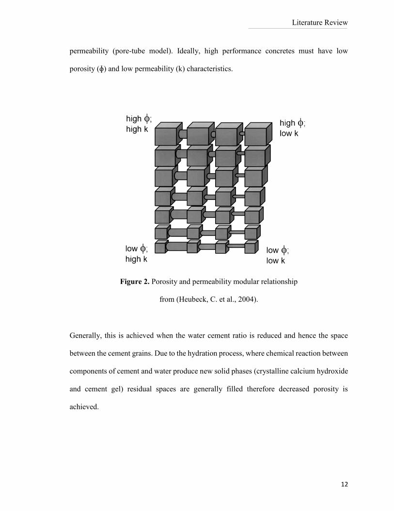
Figure 3 shows the evolution of hardening cement paste. At early stages, cement paste is
in a plastic state (cement grains immersed in water) where there are unhydrated cement
particles (A). After one hour or more, there is a reduction in water due to hydration
reactions, and subsequently, the void spaces between the cement grains are reduced, then
the void pores in the cement paste are replaced by small voids termed “gel” pores (B). The
remnants of water filled in space are known as capillary pores (large and small) but as the
hydration reaction continues, particle packing efficiency will be increased diminishing or
blocking the continuous capillary pores (C) until obtain a discontinuous pore network
which lead to a less permeable and more durable concrete.
Figure 3. Hardening procedure evolution for cement paste from
Powers et al., 1960.
Literature Review
14
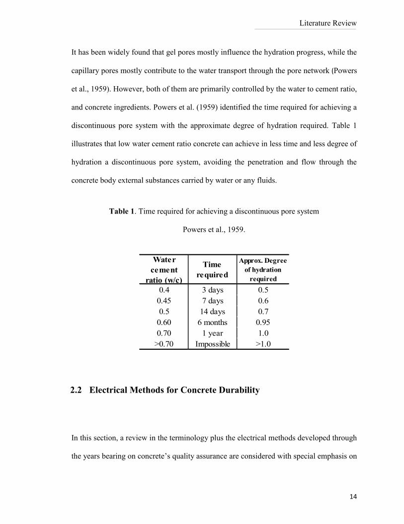
It has been widely found that gel pores mostly influence the hydration progress, while the
capillary pores mostly contribute to the water transport through the pore network (Powers
et al., 1959). However, both of them are primarily controlled by the water to cement ratio,
and concrete ingredients. Powers et al. (1959) identified the time required for achieving a
discontinuous pore system with the approximate degree of hydration required. Table 1
illustrates that low water cement ratio concrete can achieve in less time and less degree of
hydration a discontinuous pore system, avoiding the penetration and flow through the
concrete body external substances carried by water or any fluids.
2.2 Electrical Methods for Concrete Durability
In this section, a review in the terminology plus the electrical methods developed through
the years bearing on concrete’s quality assurance are considered with special emphasis on
0.4 3 days 0.5
0.45 7 days 0.6
0.5 14 days 0.7
0.60 6 months 0.95
0.70 1 year 1.0
>0.70 Impossible >1.0
Water
cement
ratio (w/c)
Time
required
Approx. Degree
of hydration
required
Table 1. Time required for achieving a discontinuous pore system
Powers et al., 1959.
Literature Review
15
the Wenner four-electrode technique (Wenner, 1916). In subsequent sections, three groups
of factors affecting test results are presented. The first group relates the factors that
influence the probe spacing. The second group presents the influences of concrete
mixtures, presence of steel reinforcing, effect of surface layer of different resistivity, and
the effect of concrete non-homogeneity on resistivity. Finally, the last group shows the
environmental effects such as temperature, moisture, and rainfall on electrical resistivity.
2.2.1 Background
During the 1920’s and 1930’s, due to concerns related to concrete durability, much interest
was being taken with the measurement of concrete properties. While, significant efforts
were made in order to measure permeability directly, the variability of replicate tests using
water, solutions or gas showed that concrete is much more variable with respect to
permeability rather than other properties such as strength. For instance, reproducible
measurements of permeability can only be made if reproducible procedures are followed
similar to testing for the 28 day strength of concrete with strictly controlled specimen
preparation (Hooton. 1989). Regardless, true permeability tests have not been standardized
and they are difficult to perform.
Concrete permeability can be measured indirectly through standard testing techniques; the
majority of them are destructive and time consuming. However, during the most recent
years, other techniques have been developed to indirectly measure this property in a non-
Literature Review
16
destructive manner, which are simple to use and not time consuming. Several studies were
conducted showing it was possible to correlate concrete’s durability with permeability, or
in other words how easy fluids and/or gases can enter into or move through the concrete
(Savas, 1999). This is due to the fact that permeability is affected by pore structure, water
cement ratio (w/c), supplementary cementitious materials, temperature, moisture degree
and other factors.
Electrical resistivity is the ability of concrete to resist electron transfer (Gowers and
Millard, 1999). Electrical resistivity measurements on saturated concrete are easier to
perform and can be related directly to permeability. In addition, such measurements have
the advantage of being non-destructive. An electrical current passes through saturated
pores containing ions from cement hydration (Shahroodi, 2010). A more tortuous path
makes it more difficult for the electrons to pass through, resulting in higher electrical
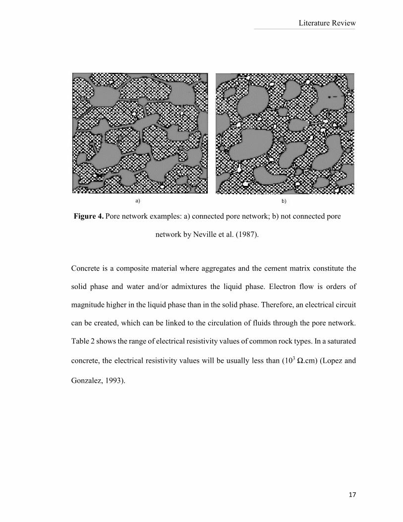
resistivity. Figure 4shows two examples of concrete pore networks; a) a network of
connected capillary pores which generates a less resistive concrete and in b) disconnected
capillary pores generating a more tortuous path leading to higher electrical resistivity.
Similar to permeability, concrete’s resistance to electrical current and transport properties
are related to its microstructure (porosity, pore connectivity and tortuosity), pore solution,
and moisture content (Elkey and Sellevold 1995; Polder et al., 1995). When a voltage is
applied, it creates an electric potential gradient that drives the flow of electrons through the
concrete; for this reason, it is possible to characterize it as a physical parameter that can be
used to indirectly characterize concrete’s permeability and hence estimate its durability.
Literature Review
17
Concrete is a composite material where aggregates and the cement matrix constitute the
solid phase and water and/or admixtures the liquid phase. Electron flow is orders of
magnitude higher in the liquid phase than in the solid phase. Therefore, an electrical circuit
can be created, which can be linked to the circulation of fluids through the pore network.
Table 2 shows the range of electrical resistivity values of common rock types. In a saturated
concrete, the electrical resistivity values will be usually less than (103 Ω.cm) (Lopez and
Gonzalez, 1993).
Figure 4. Pore network examples: a) connected pore network; b) not connected pore
network by Neville et al. (1987).
Literature Review
18
Parameters such as chloride permeability and corrosion rate of reinforcing steel can be
evaluated non-destructively by electrical resistivity, due to the fact that concrete is a semi-
conductive material. As will be described in more detail later, electrical resistivity, as
measured by AASHTO TP 95-11, can be used as an indication of concrete’s ability to resist
chloride ion penetration. Lower resistivity values indicate lower resistance to chloride
permeability.
Electrical resistivity has also been correlated to the corrosion rate of steel reinforcements
(Andrade and Alonso, 1996). Once corrosion is initiated, the corrosion rate is
approximately inversely proportional to the electrical resistivity of concrete (Hornbostel
et al., 2013). Moreover, electrical resistivity can be used to detect rebar corrosion. When
this internal process starts, an electrical circuit is formed; a corrosion current passes
through concrete from cathode to anode. Lopez and Gonalez (1993) found that steel
corrosion is inversely proportional to resistivity over a wide electrical resistivity range.
Table 3 shows the results obtained by Millard and Gowers (1991) where the electrical
resistivity was measured on concrete samples with steel reinforcement. In the study, a
Sandstone 18.0
Limestone 30.0
Marble 290.0
Granite 880.0
Type of
aggregate
Resistivity
(kΩ-cm)
Table 2. Electrical resistivity of rocks by (Monfore et al., 1968).
Literature Review
19
correlation between the corrosion level risk and resistivity was established. Low resistivity
is related to a high risk of corrosion due to the concrete’s poor ability to resist electron
transfer; hence, the pore network is not complex and is permeable allowing water ingress
more easily.
Electrical resistance is based on Ohm’s law:
𝐕 = 𝐑. 𝐈 [1]
Where, the voltage (V) is the force that drives the current through the material. It is called
voltage or the potential difference between two elements. It is expressed in volts [V]. For
instance, electrical circuits in homes have voltages of 120V/240V. The current (I) is the
amount of electricity which flows through the material, is expressed in amps [A] or in
milliamps [mA]. In common houses the electrical current is usually 100A or 200A. The
Resistance (R) is the opposition to the flow of the current (ASP Construction 2003). The
current will always seeks the easiest path; that is, the path which offers the least resistance.
For materials such as copper or aluminum, the resistance may be low since electricity to
> 20 Low rate
10 - 20 Moderate rate
5 - 10 High rate
< 5 Very high rate
Electrical
resistivity (kΩ.cm)
Corrosion
risk level
Table 3. Electrical resistivity values for rebar corrosion rate
(Millard and Gowers, 1991).
Literature Review
20
flow can pass easily through the material. For materials such as rubber, porcelain and
fiberglass, the resistance is higher impeding the electricity flow. For porous materials, the
resistivity is due to the pore network structure; granite has a higher resistance in
comparison with sandstone, as was shown in Table 2.
Electrical resistivity ρ, is an intrinsic property that normalizes the measured resistance R
and the geometry. For one dimensional flow of current, electrical resistance is normalized
by the length, L, and cross sectional area, A, as shown in equation [2].
𝝆 = 𝑹 (𝑨
𝑳) [ohm⋅cm] or [Ω. cm] [2]
Electrical conductivity is the material's ability to conduct an electric current, inversely
proportional to electrical resistivity, as shown in equation [3].
𝝈 =𝟏
𝝆 [S/m] [3]
The following sections will introduce some of these electrical techniques explaining briefly
the procedure, required testing setup, overall factors that can influence their use and finally,
disadvantages of some of these testing techniques.
2.2.2 Electrical Conductivity Tests
The Rapid Chloride Permeability test indirectly measures the concrete’s ability to resist
chloride ion penetration. The test, designated as AASHTO T277 in 1983 by the American
Literature Review
21
Association of State Highway and Transportation Officials (AASHTO), was the first-ever
test proposed for rapid qualitative assessment of chloride permeability of concrete (Chini
et al., 2003). It was later adopted by ASTM International as a standard test method for
electrical indication of concrete’s ability to resist chloride ion penetration, designated as
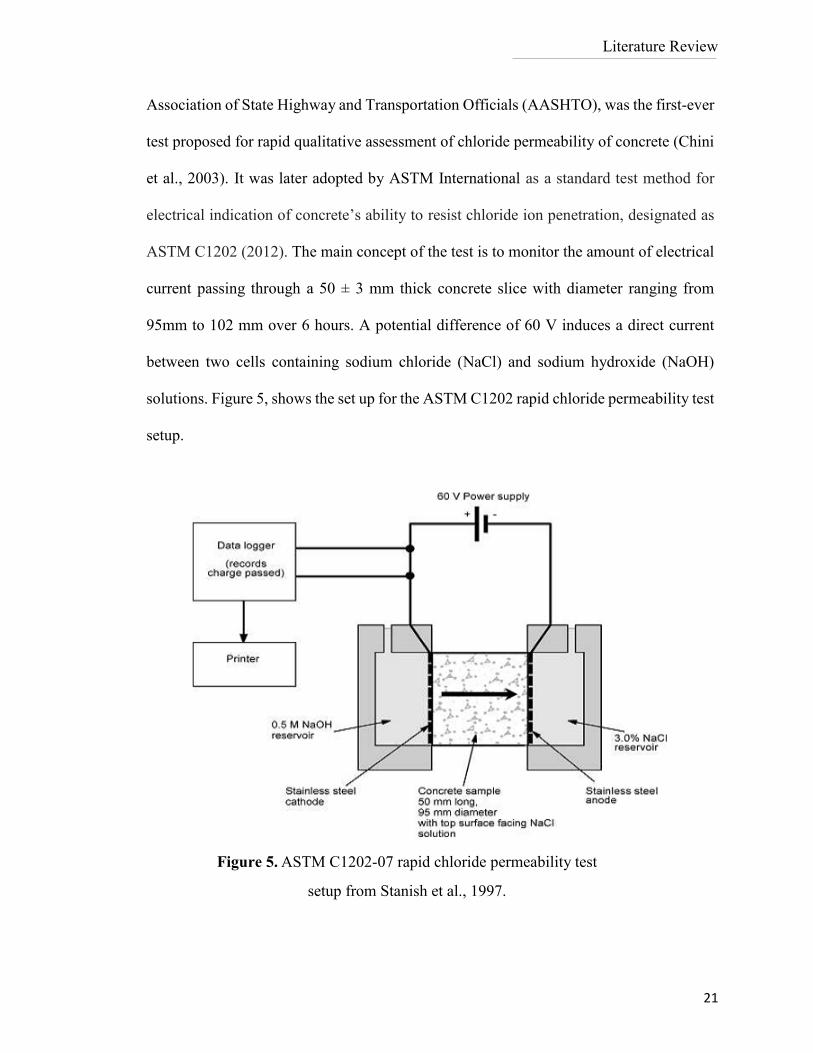
ASTM C1202 (2012). The main concept of the test is to monitor the amount of electrical
current passing through a 50 ± 3 mm thick concrete slice with diameter ranging from
95mm to 102 mm over 6 hours. A potential difference of 60 V induces a direct current
between two cells containing sodium chloride (NaCl) and sodium hydroxide (NaOH)
solutions. Figure 5, shows the set up for the ASTM C1202 rapid chloride permeability test
setup.
Figure 5. ASTM C1202-07 rapid chloride permeability test
setup from Stanish et al., 1997.
Literature Review
22
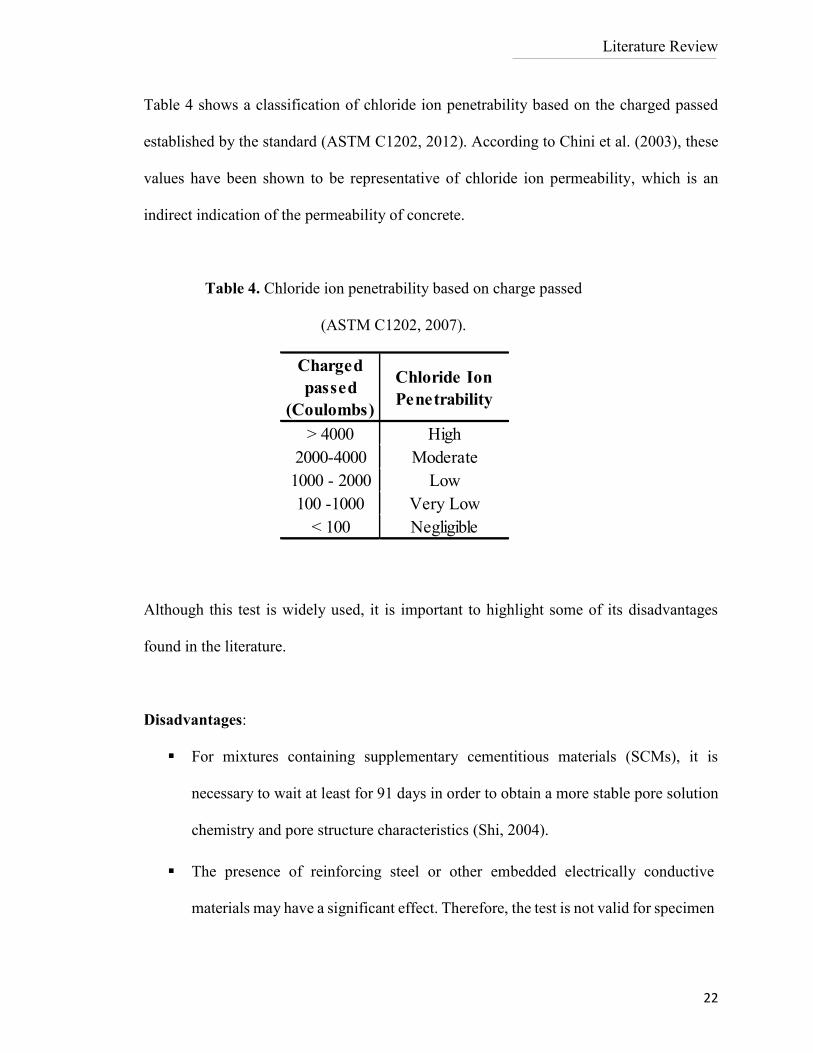
Table 4 shows a classification of chloride ion penetrability based on the charged passed
established by the standard (ASTM C1202, 2012). According to Chini et al. (2003), these
values have been shown to be representative of chloride ion permeability, which is an
indirect indication of the permeability of concrete.
Although this test is widely used, it is important to highlight some of its disadvantages
found in the literature.
Disadvantages:
For mixtures containing supplementary cementitious materials (SCMs), it is
necessary to wait at least for 91 days in order to obtain a more stable pore solution
chemistry and pore structure characteristics (Shi, 2004).
The presence of reinforcing steel or other embedded electrically conductive
materials may have a significant effect. Therefore, the test is not valid for specimen
> 4000 High
2000-4000 Moderate
1000 - 2000 Low
100 -1000 Very Low
< 100 Negligible
Charged
passed
(Coulombs)
Chloride Ion
Penetrability
Table 4. Chloride ion penetrability based on charge passed
(ASTM C1202, 2007).
Literature Review
23
with longitudinal reinforcing bars that can provide continuous electrical path
between the two ends of the specimen (ASTM C1202, 2012).
Temperature of the solution should be limited between 20 to 25 °C during
measurements. As temperature increases, the reported RCPT level of permeability
will be higher than the actual permeability level measured under the normal
temperature (Bassouni et al., 2006).
Although it is commonly referred to as the Rapid Chloride Permeability test, it
neither measures chloride diffusion or water permeability, but electrical
conductivity.
2.2.3 Electrical Resistivity Tests
In 2002, the Florida Department of Transportation (Kessler et al. 2008) started a research
program to evaluate all available electrical indicators of concrete chloride penetration
resistance in order to replace the most widely used method in the U.S., the Rapid Chloride
Permeability (RCP) test (ASTM C1202, AASHTO T277). It was found that the surface
electrical resistivity measured by an instrument called a Wenner probe without embedding
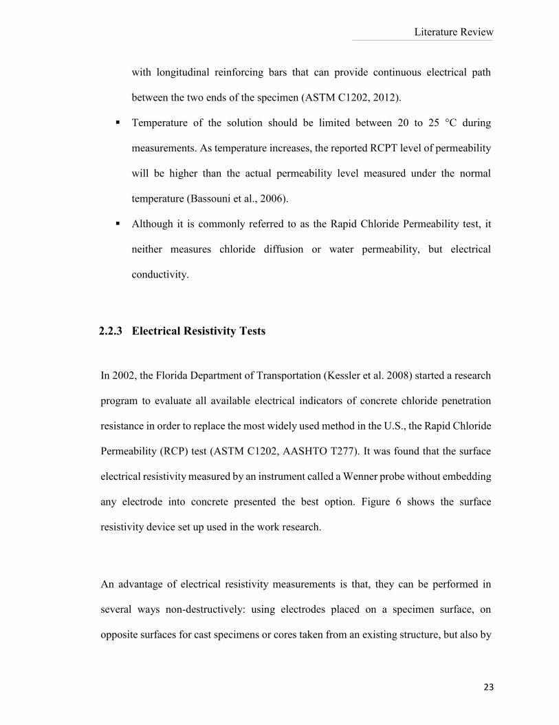
any electrode into concrete presented the best option. Figure 6 shows the surface
resistivity device set up used in the work research.
An advantage of electrical resistivity measurements is that, they can be performed in
several ways non-destructively: using electrodes placed on a specimen surface, on
opposite surfaces for cast specimens or cores taken from an existing structure, but also by
Literature Review
24
placing an electrode-disc or linear array or a four probe square array on the concrete’s
surface. A detailed description of the types of device techniques that can be used to
measure this physical property will be detailed next.
2.2.3.1 Bulk Electrical Resistivity Test
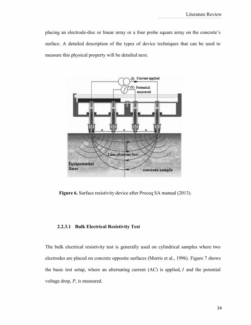
The bulk electrical resistivity test is generally used on cylindrical samples where two
electrodes are placed on concrete opposite surfaces (Morris et al., 1996). Figure 7 shows
the basic test setup, where an alternating current (AC) is applied, 𝐼 and the potential
voltage drop, P, is measured.
Figure 6. Surface resistivity device after Proceq SA manual (2013).
Literature Review
25
The electrical resistivity can be expressed as shown previously in equation [2], where, 𝜌 is
the electrical resistivity, 𝐿 is the length of the sample, 𝐴 is surface area of the specimen.
Generally this technique is used in cylinders specimens or cores taken from existing
structures.
Disadvantages:
Unfortunately, the test is not suitable to directly measure the resistivity of any
concrete element in the field, such as a column, wall or concrete beam unless the
thickness is known and accessible. However, as the electron flow is undefined,
equation 2 cannot be used to determine resistivity. In addition, Morris et al., (1996)
reported that, the use can be complicated by the need for effective and uniform
contacts between the end electrodes and concrete specimen end surfaces making it
less accurate and poorly reproducible.
It can be classified as a destructive technique due to the use of cores taken from an
existing structure.
Figure 7. Bulk Resistivity setup after Shahroodi, (2010).
Literature Review
26
Cylinders taken during casting may not accurately reflect the field concrete, so tests
on cylinders are only indicative.
2.2.3.1 Surface Electrical Resistivity
The outer layer of any concrete cast in the field produces an external layer with different
permeability in comparison with inner core concrete due to compaction, vibration,
evaporation of water and curing. This outer layer is more susceptible to aggressive
components of gases, water or chemical solutions after curing as it dries faster and results
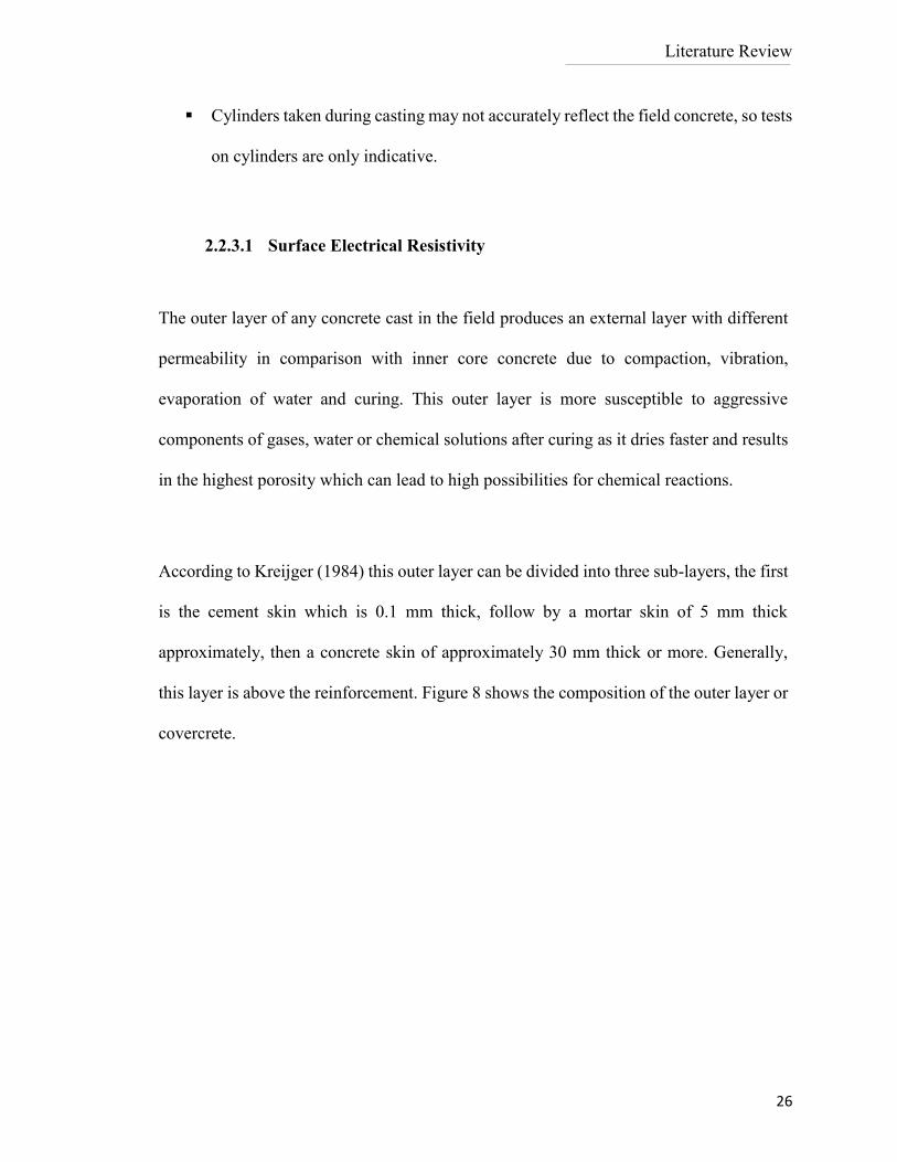
in the highest porosity which can lead to high possibilities for chemical reactions.
According to Kreijger (1984) this outer layer can be divided into three sub-layers, the first
is the cement skin which is 0.1 mm thick, follow by a mortar skin of 5 mm thick
approximately, then a concrete skin of approximately 30 mm thick or more. Generally,
this layer is above the reinforcement. Figure 8 shows the composition of the outer layer or
covercrete.
Literature Review
27
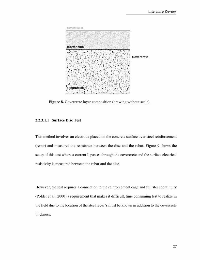
2.2.3.1.1 Surface Disc Test
This method involves an electrode placed on the concrete surface over steel reinforcement
(rebar) and measures the resistance between the disc and the rebar. Figure 9 shows the
setup of this test where a current I, passes through the covercrete and the surface electrical
resistivity is measured between the rebar and the disc.
However, the test requires a connection to the reinforcement cage and full steel continuity
(Polder et al., 2000) a requirement that makes it difficult, time consuming test to realize in
the field due to the location of the steel rebar’s must be known in addition to the covercrete
thickness.
Figure 8. Covercrete layer composition (drawing without scale).
Literature Review
28
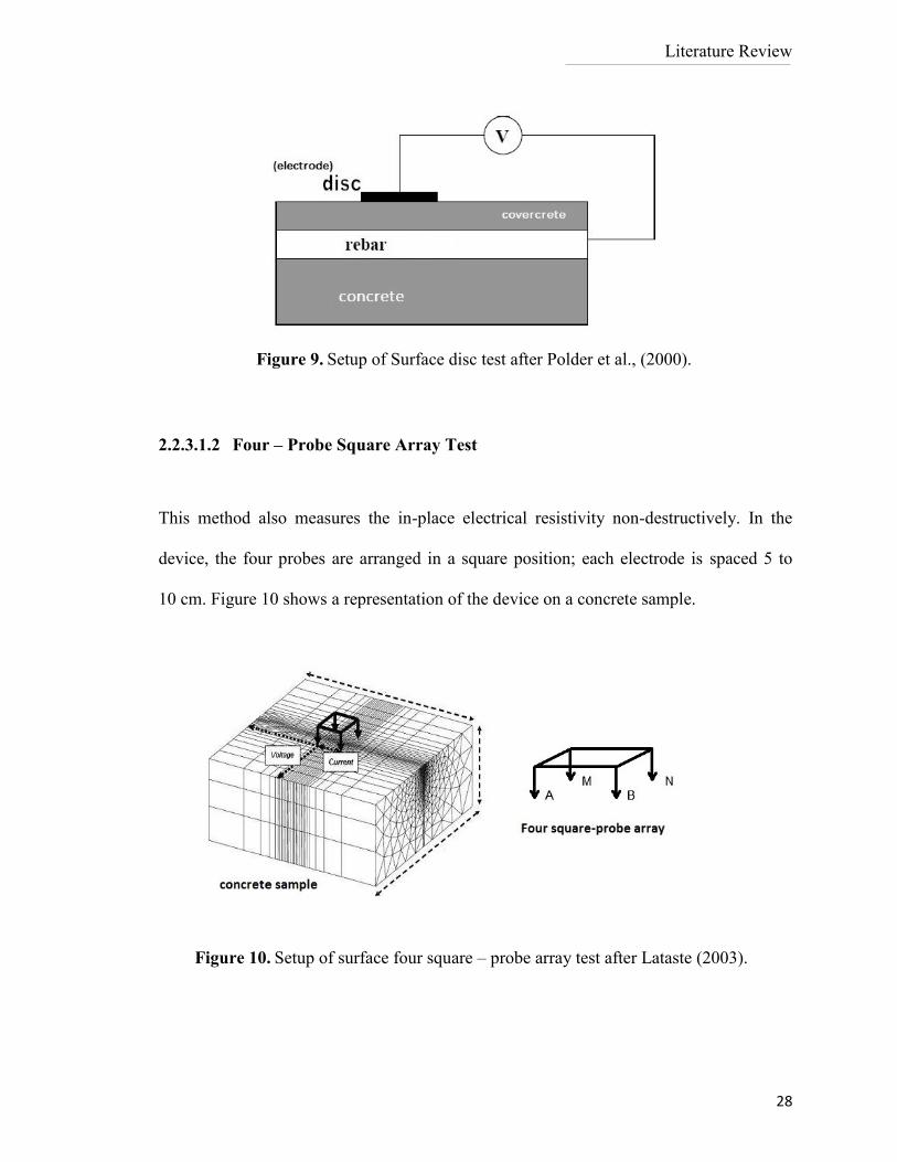
2.2.3.1.2 Four – Probe Square Array Test
This method also measures the in-place electrical resistivity non-destructively. In the
device, the four probes are arranged in a square position; each electrode is spaced 5 to
10 cm. Figure 10 shows a representation of the device on a concrete sample.
Figure 10. Setup of surface four square – probe array test after Lataste (2003).
Figure 9. Setup of Surface disc test after Polder et al., (2000).
Literature Review
29
The device works differently from the four-probe linear array device; in this case, two
neighboring electrodes (A and B) introduce a known electrical intensity while the potential
difference, ∆V created by the passage of the current in the material is measured between
the two remaining electrodes (M and N) (Lataste et al., 2003).
2.2.3.1.3 Wenner Four Probe Line Array Test
The technique was first developed for the geologist’s field in order to determine soil strata
by Frank Wenner at the National Bureau of Standards in the 1910’s and then adapted
through time for concrete use. The Wenner four-electrode probe is an instrument where
the electrodes are equally spaced on the surface of a saturated concrete element and its
main function is to measure how easily charged species in the pore solution can be
transported through the concrete under an applied electric field.
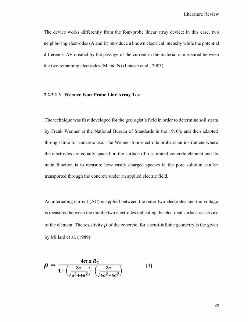
An alternating current (AC) is applied between the outer two electrodes and the voltage
is measured between the middle two electrodes indicating the electrical surface resistivity
of the element. The resistivity 𝜌 of the concrete, for a semi-infinite geometry is the given
by Millard et al. (1989).
𝝆 =𝟒𝝅 𝒂 𝑹𝑪
𝟏+ (𝟐𝒂
√𝒂𝟐+𝟒𝒅𝟐)−(
𝟐𝒂
√𝟒𝒂𝟐+𝟒𝒅𝟐) [4]
Literature Review
30
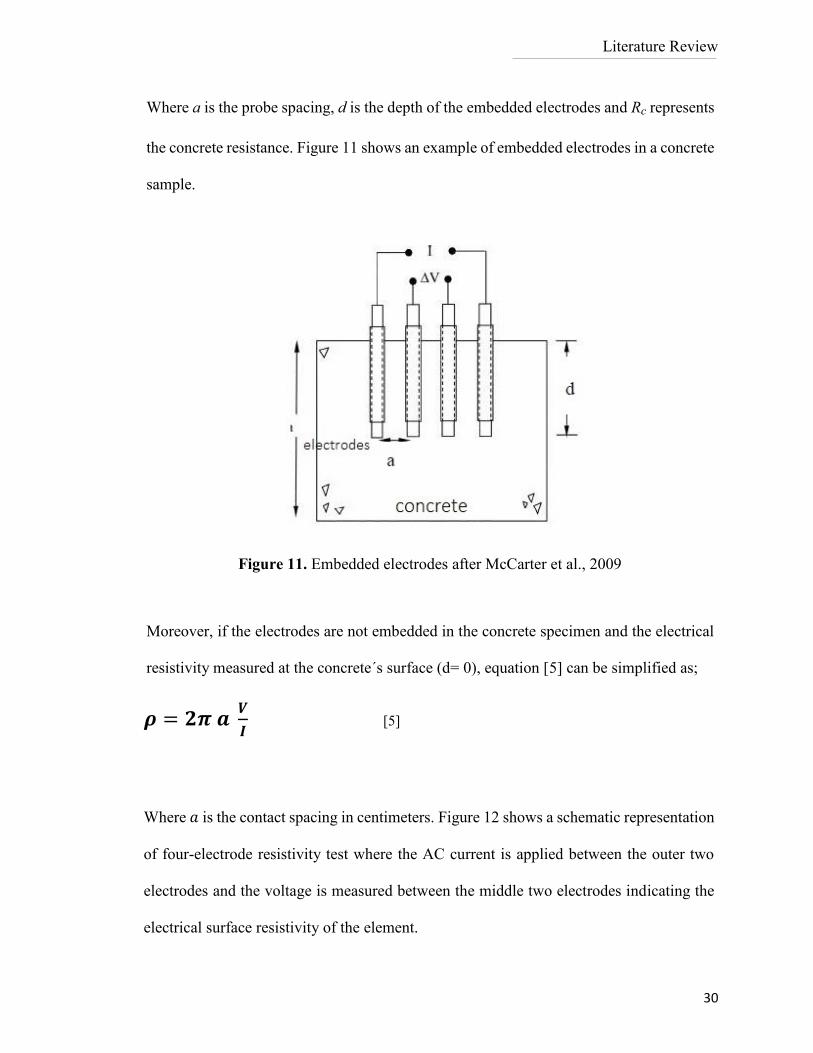
Where a is the probe spacing, d is the depth of the embedded electrodes and Rc represents
the concrete resistance. Figure 11 shows an example of embedded electrodes in a concrete
sample.
Moreover, if the electrodes are not embedded in the concrete specimen and the electrical
resistivity measured at the concrete´s surface (d= 0), equation [5] can be simplified as;
𝝆 = 𝟐𝝅 𝒂 𝑽
𝑰 [5]
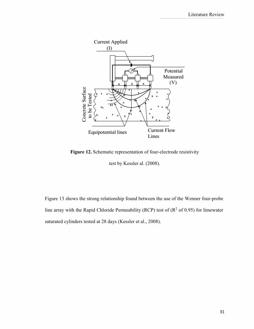
Where 𝑎 is the contact spacing in centimeters. Figure 12 shows a schematic representation
of four-electrode resistivity test where the AC current is applied between the outer two
electrodes and the voltage is measured between the middle two electrodes indicating the
electrical surface resistivity of the element.
Figure 11. Embedded electrodes after McCarter et al., 2009
Literature Review
31
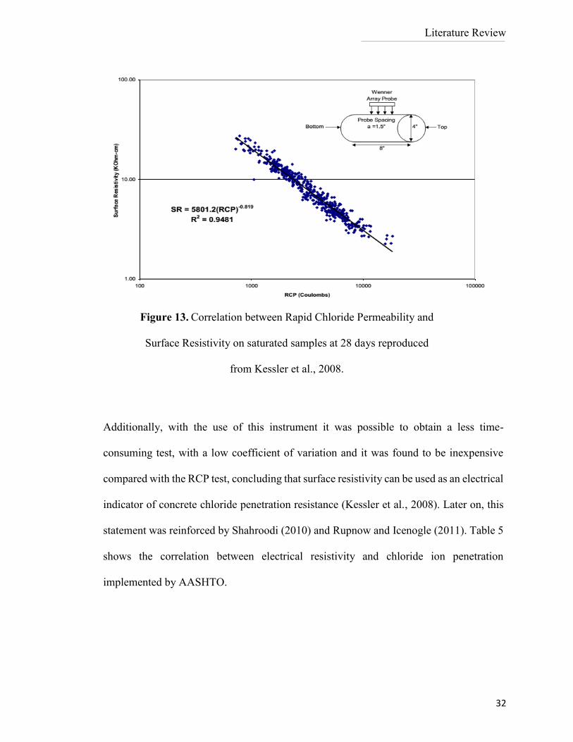
Figure 13 shows the strong relationship found between the use of the Wenner four-probe
line array with the Rapid Chloride Permeability (RCP) test of (R2 of 0.95) for limewater
saturated cylinders tested at 28 days (Kessler et al., 2008).
Figure 12. Schematic representation of four-electrode resistivity
test by Kessler al. (2008).
Literature Review
32
Additionally, with the use of this instrument it was possible to obtain a less time-
consuming test, with a low coefficient of variation and it was found to be inexpensive
compared with the RCP test, concluding that surface resistivity can be used as an electrical
indicator of concrete chloride penetration resistance (Kessler et al., 2008). Later on, this
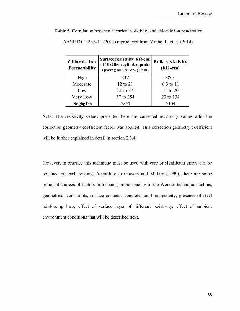
statement was reinforced by Shahroodi (2010) and Rupnow and Icenogle (2011). Table 5
shows the correlation between electrical resistivity and chloride ion penetration
implemented by AASHTO.
Figure 13. Correlation between Rapid Chloride Permeability and
Surface Resistivity on saturated samples at 28 days reproduced
from Kessler et al., 2008.
Literature Review
33
Note: The resistivity values presented here are corrected resistivity values after the
correction geometry coefficient factor was applied. This correction geometry coefficient
will be further explained in detail in section 2.3.4.
However, in practice this technique must be used with care or significant errors can be
obtained on each reading. According to Gowers and Millard (1999), there are some
principal sources of factors influencing probe spacing in the Wenner technique such as,
geometrical constraints, surface contacts, concrete non-homogeneity, presence of steel
reinforcing bars, effect of surface layer of different resistivity, effect of ambient
environment conditions that will be described next.
High <6.3
Moderate 6.3 to 11
Low 11 to 20
Very Low 20 to 134
Negligible >134
12 to 21
21 to 37
37 to 254
>254
Chloride Ion
Permeability
Bulk resistivity
(kΩ-cm)
Surface resistivity (kΩ-cm)
of 10x20cm cylinder, probe
spacing a=3.81 cm (1.5in)
<12
Table 5. Correlation between electrical resistivity and chloride ion penetration
AASHTO, TP 95-11 (2011) reproduced from Yanbo, L. et al. (2014).
Literature Review
34
2.3 Factors Influencing Probe Spacing in the Wenner Four Probe
Technique
It was found there are some influences regarding use of resistivity measurements that easily
can be avoided but some others are more complex. This first set of parameters is directly
related with the use of the Wenner four probe device: the influence of the use of different
probe spacing, the effect of surface contacts between the probe tips and concrete, the
geometrical constraints found on cylindrical samples, and the specimen geometry.
2.3.1 Surface Contacts
Full contact between the Wenner four probe device and the surface must be applied to
obtain reliable measurements. This is particularly important for the two inner contacts
measuring the potential difference. An uneven electrical contact generates unreliable
values. According to Gowers and Millard (1999), the use of a relatively low frequency and
alternating current (AC) helps to minimize misleading values. The use of a direct current
(DC) signal lead to problems due to polarization effects at the surface contacts.
Literature Review
35
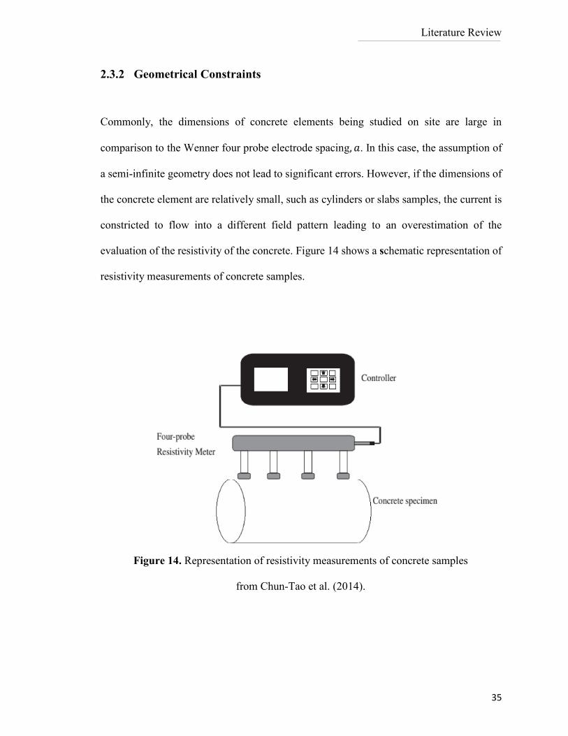
2.3.2 Geometrical Constraints
Commonly, the dimensions of concrete elements being studied on site are large in
comparison to the Wenner four probe electrode spacing, 𝑎. In this case, the assumption of
a semi-infinite geometry does not lead to significant errors. However, if the dimensions of
the concrete element are relatively small, such as cylinders or slabs samples, the current is
constricted to flow into a different field pattern leading to an overestimation of the
evaluation of the resistivity of the concrete. Figure 14 shows a schematic representation of
resistivity measurements of concrete samples.
Figure 14. Representation of resistivity measurements of concrete samples
from Chun-Tao et al. (2014).
Literature Review
36
According to (Gowers and Millard 1999) through experimental findings, the contact
spacing should not exceed ¼ of the concrete section dimensions. The distance of the
contacts from any element edge should also be at least twice the contact spacing. When the
test is conducted on cylindrical specimens, the semi-infinite assumption is not valid as the
large probe spacing and the small geometry generates a flow interfering with coarse
aggregates, necessitating estimating a factor to account for the constricted flow in the
material. Spragg et al. (2013a) established the following correction coefficient factor (k),
equation [6], using the simulations developed by Morris et al. (1996).
𝒌 = 𝟏. 𝟏𝟎 − 𝟎.𝟕𝟑𝟎
𝐝𝐚⁄
+ 𝟕.𝟑𝟒
(𝐝𝐚⁄ )
𝟐 [6]
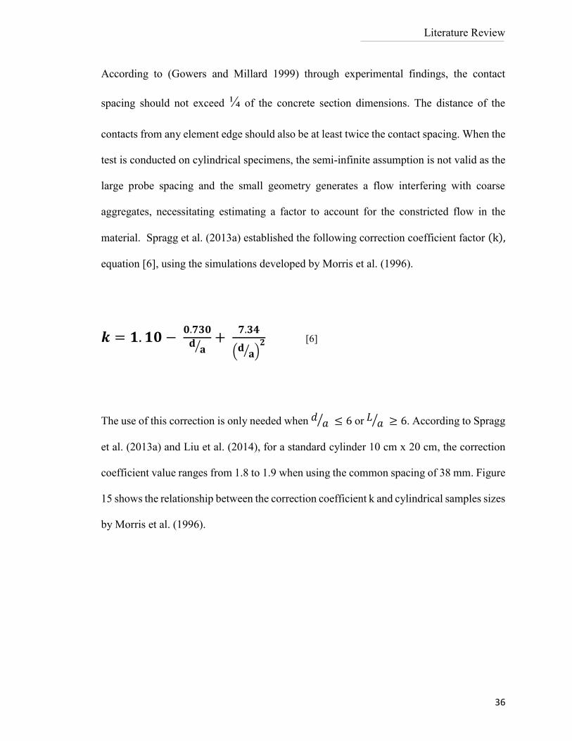
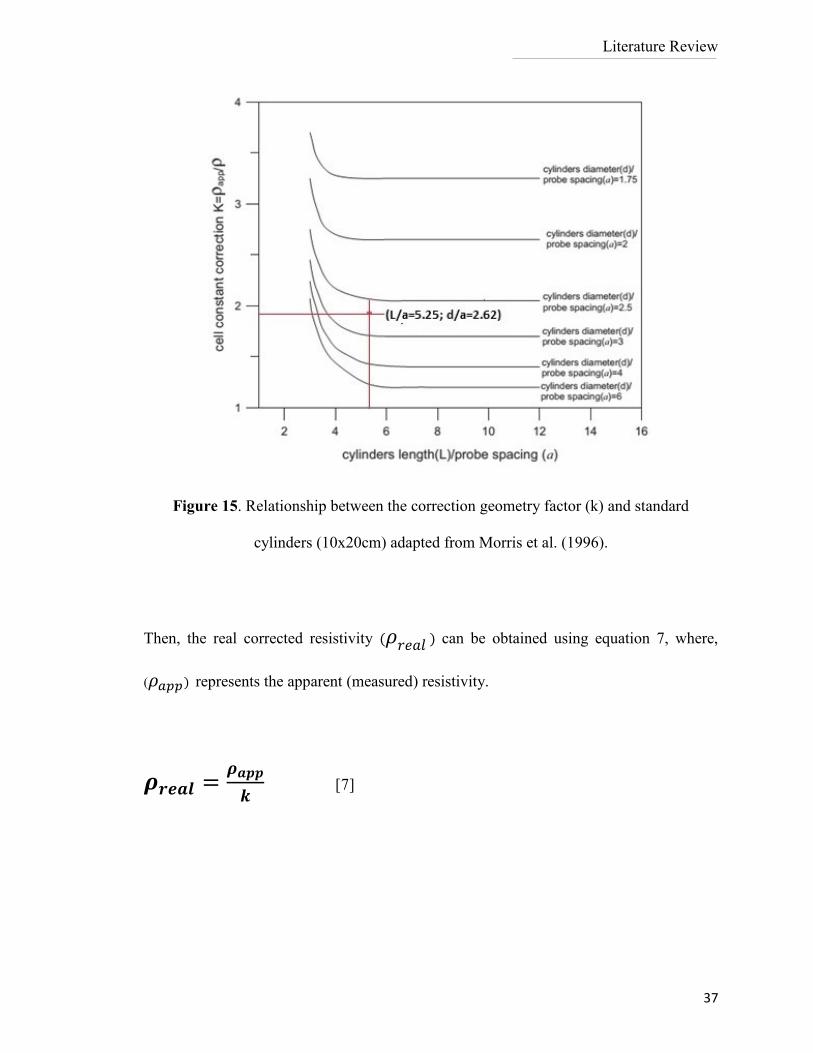
The use of this correction is only needed when 𝑑 𝑎⁄ ≤ 6 or 𝐿 𝑎⁄ ≥ 6. According to Spragg
et al. (2013a) and Liu et al. (2014), for a standard cylinder 10 cm x 20 cm, the correction
coefficient value ranges from 1.8 to 1.9 when using the common spacing of 38 mm. Figure
15 shows the relationship between the correction coefficient k and cylindrical samples sizes
by Morris et al. (1996).
Literature Review
37
Then, the real corrected resistivity (𝜌𝑟𝑒𝑎𝑙 ) can be obtained using equation 7, where,
(𝜌𝑎𝑝𝑝) represents the apparent (measured) resistivity.
𝝆𝒓𝒆𝒂𝒍 =𝝆𝒂𝒑𝒑
𝒌 [7]
Figure 15. Relationship between the correction geometry factor (k) and standard
cylinders (10x20cm) adapted from Morris et al. (1996).
Literature Review
38
2.3.3 Probe Spacing
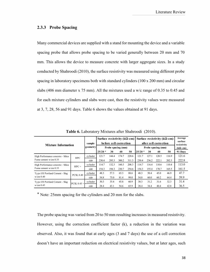
Many commercial devices are supplied with a stand for mounting the device and a variable
spacing probe that allows probe spacing to be varied generally between 20 mm and 70
mm. This allows the device to measure concrete with larger aggregate sizes. In a study
conducted by Shahroodi (2010), the surface resistivity was measured using different probe
spacing in laboratory specimens both with standard cylinders (100 x 200 mm) and circular
slabs (406 mm diameter x 75 mm). All the mixtures used a w/c range of 0.35 to 0.45 and
for each mixture cylinders and slabs were cast, then the resistivity values were measured
at 3, 7, 28, 56 and 91 days. Table 6 shows the values obtained at 91 days.
Note: 25mm spacing for the cylinders and 20 mm for the slabs.
The probe spacing was varied from 20 to 50 mm resulting increases in measured resistivity.
However, using the correction coefficient factor (k), a reduction in the variation was
observed. Also, it was found that at early ages (3 and 7 days) the use of a cell correction
doesn’t have an important reduction on electrical resistivity values, but at later ages, such
25/20 * 30 40 50 25/20 * 30 40 50 91 Days
cylinder 121.7 144.4 174.7 220.6 121.7 127.1 120.5 116.9 121.6
slab 230.4 295.3 300.2 311.3 230.4 236.2 222.1 202.3 222.8
cylinder 114.7 132.3 160.3 208.3 114.7 116.4 110.6 110.4 113.0
slab 154.3 194.3 230.7 254.6 154.3 155.4 170.7 165.5 161.5
cylinder 48.3 57.3 65.3 88.6 48.3 50.4 45.0 46.9 47.7
slab 54.8 75.0 81.4 99.0 54.8 60.0 60.2 64.4 59.9
cylinder 30.3 35.4 45.8 60.9 30.3 31.2 31.6 32.3 31.4
slab 28.4 43.1 54.6 65.9 28.4 34.4 40.4 42.8 36.5
Average
surface
resistivity
(kΩ- cm)
Type I/II Portland Cement - Slag
w/cm 0.45PCSL 0.45 +
High Performance concrete - Silica
Fume cement w/cm 0.35HPC +
Type I/II Portland Cement - Slag
w/cm 0.40PCSL 0.40
High Performance concrete - Silica
Fume cement w/cm 0.35HPC
Probe spacing (mm)
sample
geometryMixture Information
Surface resistivity (kΩ-cm)
after cell correction
Surface resistivity (kΩ-cm)
before cell correction
Probe spacing (mm)
Table 6. Laboratory Mixtures after Shahroodi (2010).
Literature Review
39
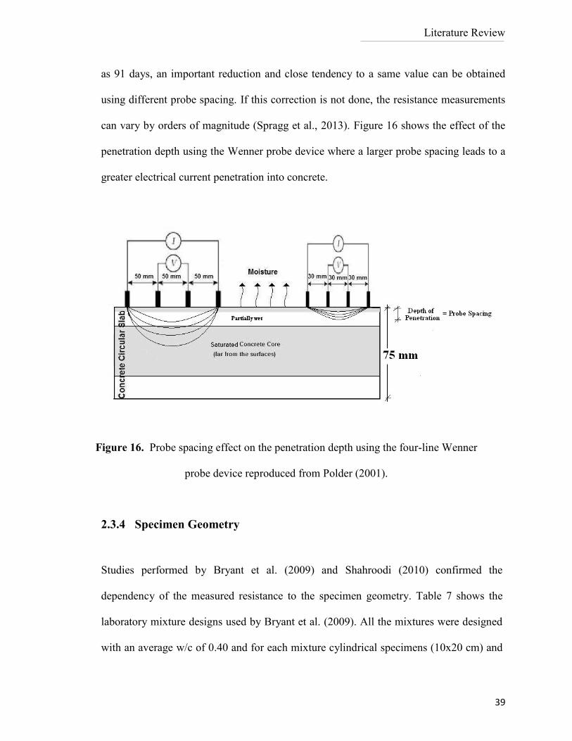
as 91 days, an important reduction and close tendency to a same value can be obtained
using different probe spacing. If this correction is not done, the resistance measurements
can vary by orders of magnitude (Spragg et al., 2013). Figure 16 shows the effect of the
penetration depth using the Wenner probe device where a larger probe spacing leads to a
greater electrical current penetration into concrete.
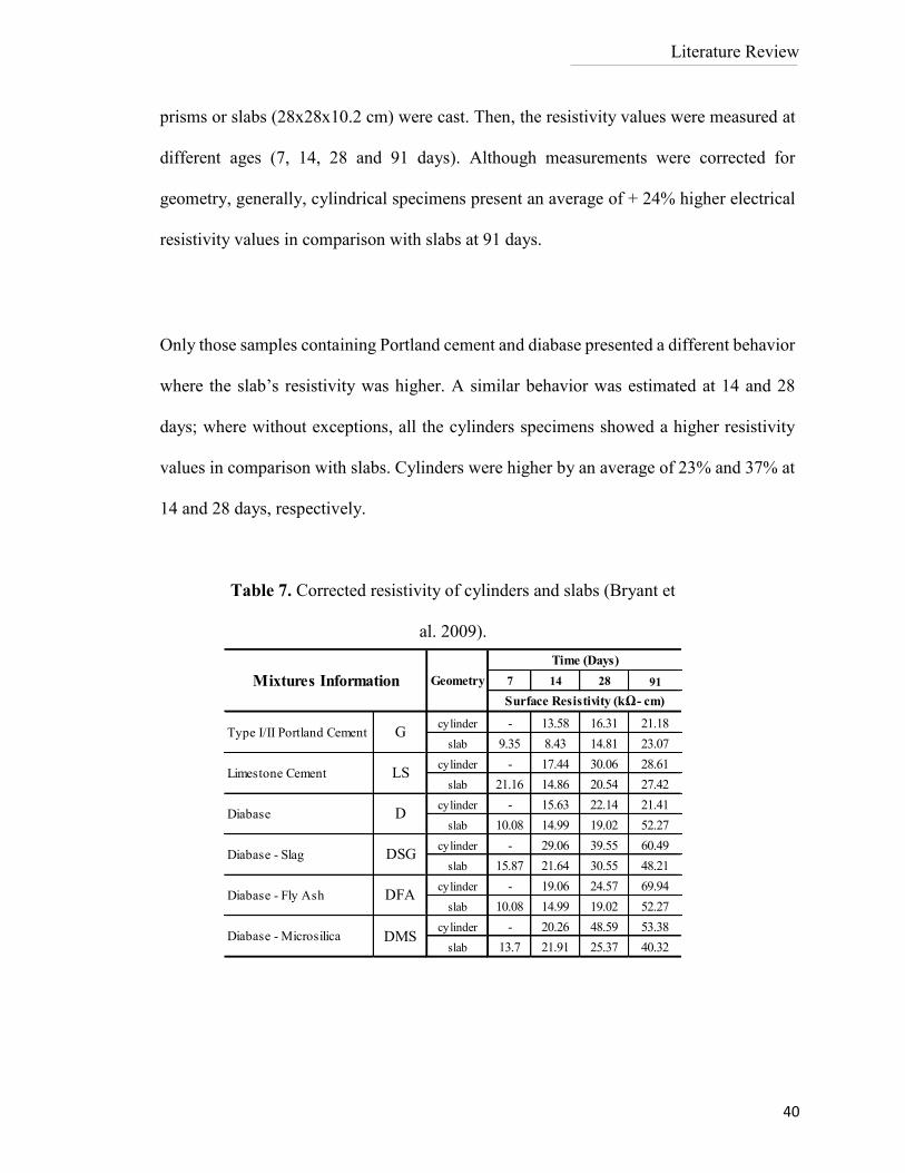
2.3.4 Specimen Geometry
Studies performed by Bryant et al. (2009) and Shahroodi (2010) confirmed the
dependency of the measured resistance to the specimen geometry. Table 7 shows the
laboratory mixture designs used by Bryant et al. (2009). All the mixtures were designed
with an average w/c of 0.40 and for each mixture cylindrical specimens (10x20 cm) and
Figure 16. Probe spacing effect on the penetration depth using the four-line Wenner
probe device reproduced from Polder (2001).
Literature Review
40
prisms or slabs (28x28x10.2 cm) were cast. Then, the resistivity values were measured at
different ages (7, 14, 28 and 91 days). Although measurements were corrected for
geometry, generally, cylindrical specimens present an average of + 24% higher electrical
resistivity values in comparison with slabs at 91 days.
Only those samples containing Portland cement and diabase presented a different behavior
where the slab’s resistivity was higher. A similar behavior was estimated at 14 and 28
days; where without exceptions, all the cylinders specimens showed a higher resistivity
values in comparison with slabs. Cylinders were higher by an average of 23% and 37% at
14 and 28 days, respectively.
7 14 28 91
cylinder - 13.58 16.31 21.18
slab 9.35 8.43 14.81 23.07
cylinder - 17.44 30.06 28.61
slab 21.16 14.86 20.54 27.42
cylinder - 15.63 22.14 21.41
slab 10.08 14.99 19.02 52.27
cylinder - 29.06 39.55 60.49
slab 15.87 21.64 30.55 48.21
cylinder - 19.06 24.57 69.94
slab 10.08 14.99 19.02 52.27
cylinder - 20.26 48.59 53.38
slab 13.7 21.91 25.37 40.32
Diabase - Slag DSG
Diabase - Fly Ash DFA
Diabase - Microsilica DMS
Type I/II Portland Cement G
Limestone Cement LS
Diabase D
Mixtures Information Geometry
Time (Days)
Surface Resistivity (kΩ- cm)
Table 7. Corrected resistivity of cylinders and slabs (Bryant et
al. 2009).
Literature Review
41
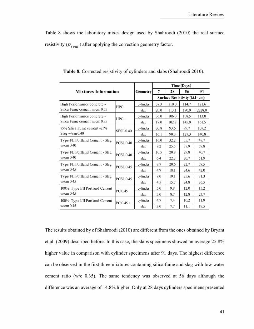
Table 8 shows the laboratory mixes design used by Shahroodi (2010) the real surface
resistivity (𝜌𝑟𝑒𝑎𝑙 ) after applying the correction geometry factor.
The results obtained by of Shahroodi (2010) are different from the ones obtained by Bryant
et al. (2009) described before. In this case, the slabs specimens showed an average 25.8%
higher value in comparison with cylinder specimens after 91 days. The highest difference
can be observed in the first three mixtures containing silica fume and slag with low water
cement ratio (w/c 0.35). The same tendency was observed at 56 days although the
difference was an average of 14.8% higher. Only at 28 days cylinders specimens presented
7 28 56 91
cylinder 37.3 110.0 114.7 121.6
slab 20.0 113.1 190.9 2228.0
cylinder 36.0 106.0 108.5 113.0
slab 17.0 102.8 145.9 161.5
cylinder 30.8 93.6 99.7 107.2
slab 16.1 90.8 127.3 140.8
cylinder 16.0 32.2 35.7 47.7
slab 8.2 25.5 37.9 59.8
cylinder 10.5 20.8 29.8 40.7
slab 6.4 22.3 30.7 51.9
cylinder 8.7 20.6 22.7 39.5
slab 4.9 18.1 24.6 42.0
cylinder 8.0 19.1 25.6 31.3
slab 4.5 15.7 24.8 36.5
cylinder 5.0 9.8 12.0 15.2
slab 3.0 8.7 12.8 23.7
cylinder 4.7 7.4 10.2 11.9
slab 3.0 7.7 11.1 19.5
100% Type I/II Portland Cement
w/cm 0.45PC 0.45
100% Type I/II Portland Cement
w/cm 0.45PC 0.45 +
Type I/II Portland Cement - Slag
w/cm 0.40PCSL 0.40 +
Type I/II Portland Cement - Slag
w/cm 0.45PCSL 0.45
Type I/II Portland Cement - Slag
w/cm 0.45PCSL 0.45 +
High Performance concrete -
Silica Fume cement w/cm 0.35HPC +
75% Silica Fume cement -25%
Slag w/cm 0.40SFSL 0.40
Type I/II Portland Cement - Slag
w/cm 0.40PCSL 0.40
Mixtures Information Geometry
Time (Days)
Surface Resistivity (kΩ- cm)
High Performance concrete -
Silica Fume cement w/cm 0.35HPC
Table 8. Corrected resistivity of cylinders and slabs (Shahroodi 2010).
Literature Review
42
an average of 13% higher resistivity but only for the mixtures HPC+, SFSL 0.40, PCSL
0.40, PCSL 0.45 PCSL 0.45+ and PC 0.45.
Some alternatives can be presented as possible explanations for the difference in the two
studies. The first one is the geometry correction coefficient described previously in section
2.3.2 in order to avoid the overestimation in the electrical values due to the size sample.
Another factor is the surface texture, which is important according to Bryant et al. (2009).
The cylinders are always tested on the cast surface along its height (more uniform and
smoother) than the rough finished surface presented in the prism or slabs specimens. The
variability can be reduced by abrading the surface to a smoother surface and/or material
of the resistivity meter contact probes. Lastly, the variability associated with Wenner probe
test arises mainly from factors as, the device, operator, material, production and curing
process and they can be represented in the following expression (Equation 8, Spragg et al.,
2013). Although in this research the variables were constant (device, operator, production
and curing), in cases where this cannot be achieved, it is an important consideration.
𝝈𝒕𝒐𝒕𝒂𝒍 = √𝝈𝒎𝒂𝒄𝒉𝒊𝒏𝒆𝟐 + 𝝈𝒐𝒑𝒆𝒓𝒂𝒕𝒐𝒓
𝟐 + 𝝈𝒎𝒂𝒕𝒆𝒓𝒊𝒂𝒍𝟐 + 𝝈𝒑𝒓𝒐𝒅𝒖𝒄𝒕𝒊𝒐𝒏
𝟐 + 𝝈𝒄𝒖𝒓𝒊𝒏𝒈𝟐 [8]
According to Spragg et al. (2013) it was estimated from laboratory conditions the
variability of machine, operator, and material as 1.7%, 1.8%, and 3.4%, respectively due
to the repeatability; matching with the findings of Rupnow and Icenogle et al. (2011).
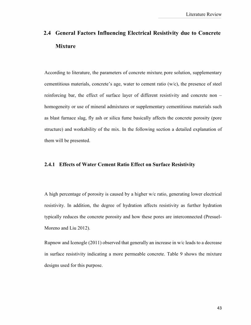
Literature Review
43
2.4 General Factors Influencing Electrical Resistivity due to Concrete
Mixture
According to literature, the parameters of concrete mixture, pore solution, supplementary
cementitious materials, concrete’s age, water to cement ratio (w/c), the presence of steel
reinforcing bar, the effect of surface layer of different resistivity and concrete non –
homogeneity or use of mineral admixtures or supplementary cementitious materials such
as blast furnace slag, fly ash or silica fume basically affects the concrete porosity (pore
structure) and workability of the mix. In the following section a detailed explanation of
them will be presented.
2.4.1 Effects of Water Cement Ratio Effect on Surface Resistivity
A high percentage of porosity is caused by a higher w/c ratio, generating lower electrical
resistivity. In addition, the degree of hydration affects resistivity as further hydration
typically reduces the concrete porosity and how these pores are interconnected (Presuel-
Moreno and Liu 2012).
Rupnow and Icenogle (2011) observed that generally an increase in w/c leads to a decrease
in surface resistivity indicating a more permeable concrete. Table 9 shows the mixture
designs used for this purpose.
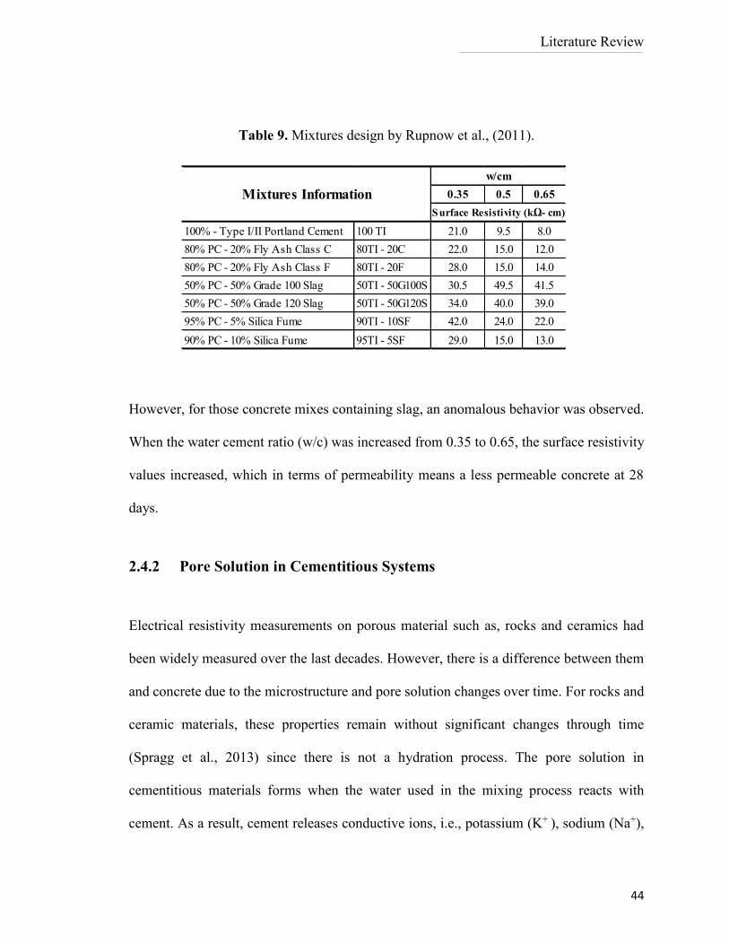
Literature Review
44
However, for those concrete mixes containing slag, an anomalous behavior was observed.
When the water cement ratio (w/c) was increased from 0.35 to 0.65, the surface resistivity
values increased, which in terms of permeability means a less permeable concrete at 28
days.
2.4.2 Pore Solution in Cementitious Systems
Electrical resistivity measurements on porous material such as, rocks and ceramics had
been widely measured over the last decades. However, there is a difference between them
and concrete due to the microstructure and pore solution changes over time. For rocks and
ceramic materials, these properties remain without significant changes through time
(Spragg et al., 2013) since there is not a hydration process. The pore solution in
cementitious materials forms when the water used in the mixing process reacts with
cement. As a result, cement releases conductive ions, i.e., potassium (K+ ), sodium (Na+),
0.35 0.5 0.65
100% - Type I/II Portland Cement 100 TI 21.0 9.5 8.0
80% PC - 20% Fly Ash Class C 80TI - 20C 22.0 15.0 12.0
80% PC - 20% Fly Ash Class F 80TI - 20F 28.0 15.0 14.0
50% PC - 50% Grade 100 Slag 50TI - 50G100S 30.5 49.5 41.5
50% PC - 50% Grade 120 Slag 50TI - 50G120S 34.0 40.0 39.0
95% PC - 5% Silica Fume 90TI - 10SF 42.0 24.0 22.0
90% PC - 10% Silica Fume 95TI - 5SF 29.0 15.0 13.0
Mixtures Information
w/cm
Surface Resistivity (kΩ- cm)
Table 9. Mixtures design by Rupnow et al., (2011).
Literature Review
45
calcium (Ca2+), hydroxide (OH-), and sulfate (SO42-) into the pore solution. (Barneyback
and Diamond 1981; Elkey and Sellevold 1995; McCarter 1996). However, the amount of
conductive ions released depends on the chemistry of the cement, the water used in the
mixing process and the hydration degree of the cementitious materials (Spragg et al., 2013).
Figure 17 shows a schematic representation of the ion conductivity in porous materials.
Porosity can be described as the volume of pores in the system and the connectivity
characterizes the way pores are connected through the three-dimensional system or the
concrete’s pore network (Spragg et al., 2013).
Figure 17. Conductivity in porous material, a) ions released in the pore solution; b)
porosity; c) connectivity, reproduced from Spragg et al. (2013).
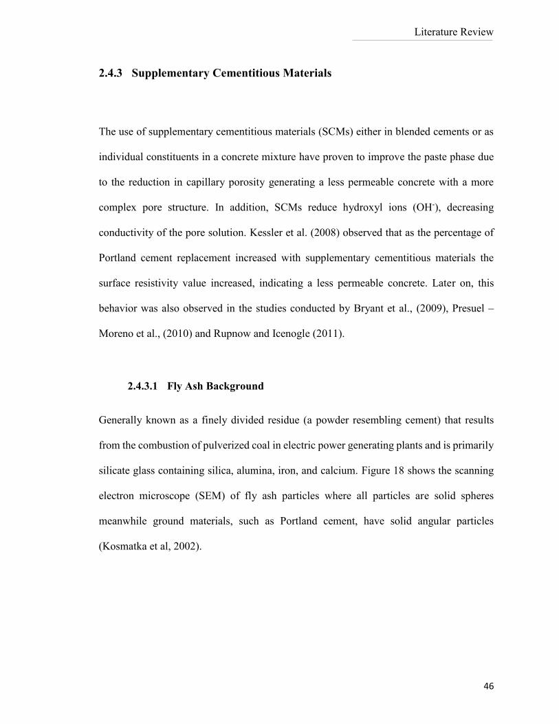
Literature Review
46
2.4.3 Supplementary Cementitious Materials
The use of supplementary cementitious materials (SCMs) either in blended cements or as
individual constituents in a concrete mixture have proven to improve the paste phase due
to the reduction in capillary porosity generating a less permeable concrete with a more
complex pore structure. In addition, SCMs reduce hydroxyl ions (OH-), decreasing
conductivity of the pore solution. Kessler et al. (2008) observed that as the percentage of
Portland cement replacement increased with supplementary cementitious materials the
surface resistivity value increased, indicating a less permeable concrete. Later on, this
behavior was also observed in the studies conducted by Bryant et al., (2009), Presuel –
Moreno et al., (2010) and Rupnow and Icenogle (2011).
2.4.3.1 Fly Ash Background
Generally known as a finely divided residue (a powder resembling cement) that results
from the combustion of pulverized coal in electric power generating plants and is primarily
silicate glass containing silica, alumina, iron, and calcium. Figure 18 shows the scanning
electron microscope (SEM) of fly ash particles where all particles are solid spheres
meanwhile ground materials, such as Portland cement, have solid angular particles
(Kosmatka et al, 2002).
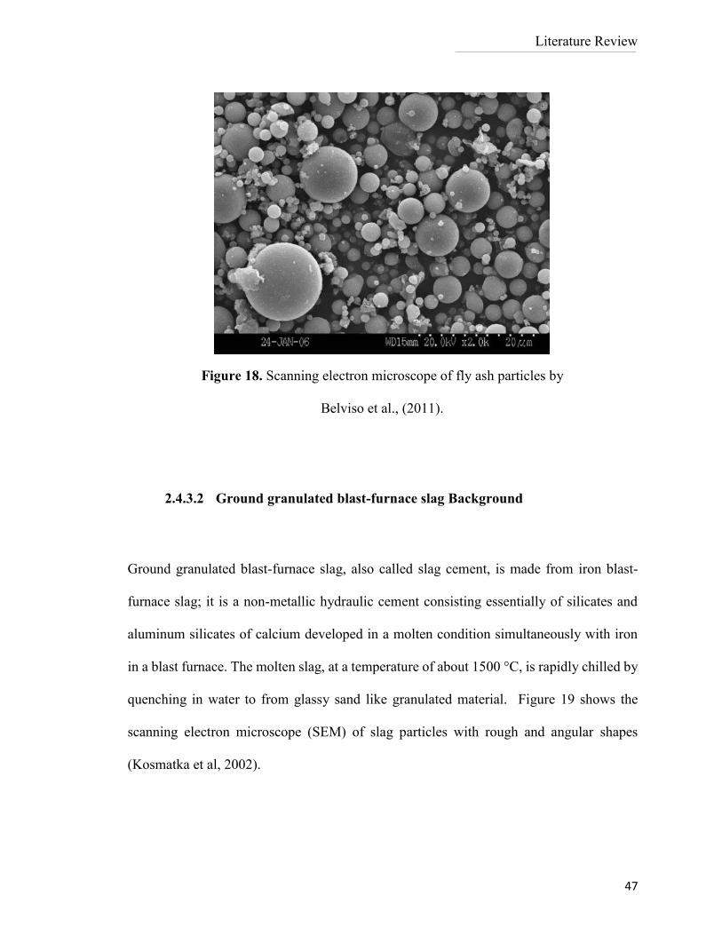
Literature Review
47
2.4.3.2 Ground granulated blast-furnace slag Background
Ground granulated blast-furnace slag, also called slag cement, is made from iron blast-
furnace slag; it is a non-metallic hydraulic cement consisting essentially of silicates and
aluminum silicates of calcium developed in a molten condition simultaneously with iron
in a blast furnace. The molten slag, at a temperature of about 1500 °C, is rapidly chilled by
quenching in water to from glassy sand like granulated material. Figure 19 shows the
scanning electron microscope (SEM) of slag particles with rough and angular shapes
(Kosmatka et al, 2002).
Figure 18. Scanning electron microscope of fly ash particles by
Belviso et al., (2011).
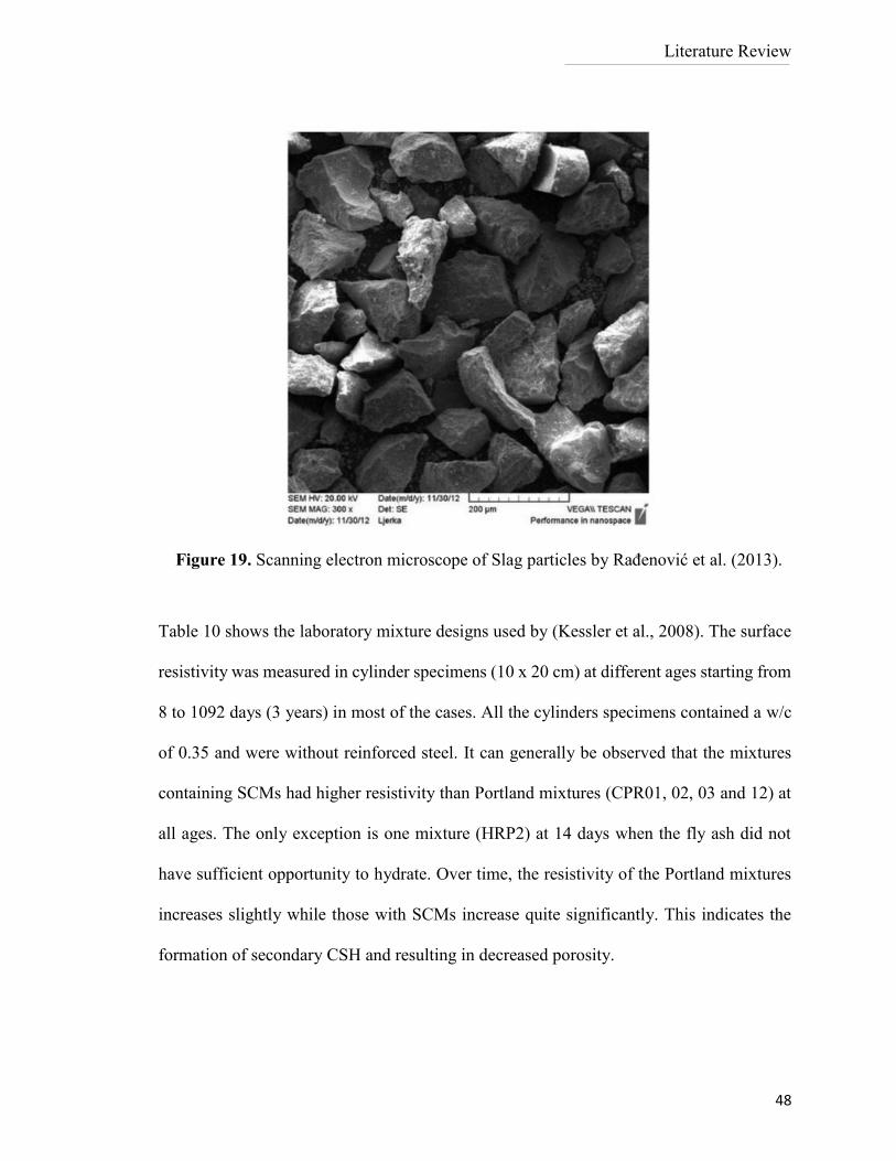
Literature Review
48
Table 10 shows the laboratory mixture designs used by (Kessler et al., 2008). The surface
resistivity was measured in cylinder specimens (10 x 20 cm) at different ages starting from
8 to 1092 days (3 years) in most of the cases. All the cylinders specimens contained a w/c
of 0.35 and were without reinforced steel. It can generally be observed that the mixtures
containing SCMs had higher resistivity than Portland mixtures (CPR01, 02, 03 and 12) at
all ages. The only exception is one mixture (HRP2) at 14 days when the fly ash did not
have sufficient opportunity to hydrate. Over time, the resistivity of the Portland mixtures
increases slightly while those with SCMs increase quite significantly. This indicates the
formation of secondary CSH and resulting in decreased porosity.
Figure 19. Scanning electron microscope of Slag particles by Rađenović et al. (2013).
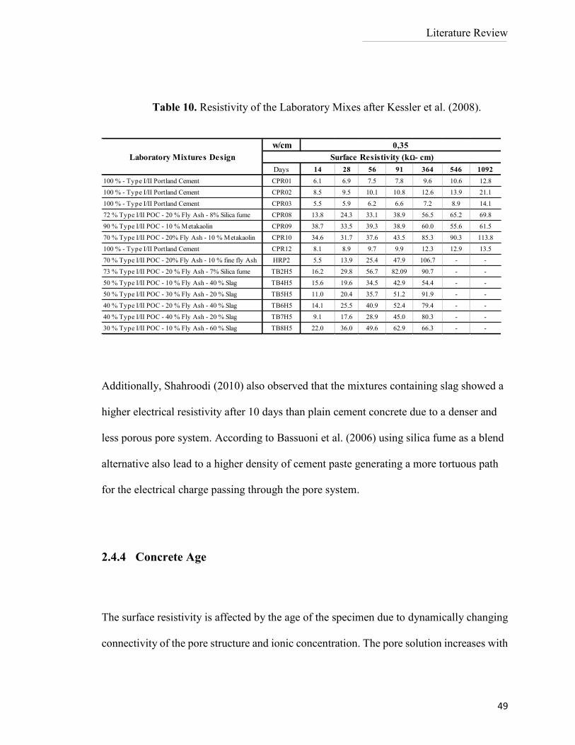
Literature Review
49
Additionally, Shahroodi (2010) also observed that the mixtures containing slag showed a
higher electrical resistivity after 10 days than plain cement concrete due to a denser and
less porous pore system. According to Bassuoni et al. (2006) using silica fume as a blend
alternative also lead to a higher density of cement paste generating a more tortuous path
for the electrical charge passing through the pore system.
2.4.4 Concrete Age
The surface resistivity is affected by the age of the specimen due to dynamically changing
connectivity of the pore structure and ionic concentration. The pore solution increases with
w/cm
Days 14 28 56 91 364 546 1092
100 % - Type I/II Portland Cement CPR01 6.1 6.9 7.5 7.8 9.6 10.6 12.8
100 % - Type I/II Portland Cement CPR02 8.5 9.5 10.1 10.8 12.6 13.9 21.1
100 % - Type I/II Portland Cement CPR03 5.5 5.9 6.2 6.6 7.2 8.9 14.1
72 % Type I/II POC - 20 % Fly Ash - 8% Silica fume CPR08 13.8 24.3 33.1 38.9 56.5 65.2 69.8
90 % Type I/II POC - 10 % Metakaolin CPR09 38.7 33.5 39.3 38.9 60.0 55.6 61.5
70 % Type I/II POC - 20% Fly Ash - 10 % Metakaolin CPR10 34.6 31.7 37.6 43.5 85.3 90.3 113.8
100 % - Type I/II Portland Cement CPR12 8.1 8.9 9.7 9.9 12.3 12.9 13.5
70 % Type I/II POC - 20% Fly Ash - 10 % fine fly Ash HRP2 5.5 13.9 25.4 47.9 106.7 - -
73 % Type I/II POC - 20 % Fly Ash - 7% Silica fume TB2H5 16.2 29.8 56.7 82.09 90.7 - -
50 % Type I/II POC - 10 % Fly Ash - 40 % Slag TB4H5 15.6 19.6 34.5 42.9 54.4 - -
50 % Type I/II POC - 30 % Fly Ash - 20 % Slag TB5H5 11.0 20.4 35.7 51.2 91.9 - -
40 % Type I/II POC - 20 % Fly Ash - 40 % Slag TB6H5 14.1 25.5 40.9 52.4 79.4 - -
40 % Type I/II POC - 40 % Fly Ash - 20 % Slag TB7H5 9.1 17.6 28.9 45.0 80.3 - -
30 % Type I/II POC - 10 % Fly Ash - 60 % Slag TB8H5 22.0 36.0 49.6 62.9 66.3 - -
Laboratory Mixtures Design
0,35
Surface Resistivity (kΩ- cm)
Table 10. Resistivity of the Laboratory Mixes after Kessler et al. (2008).
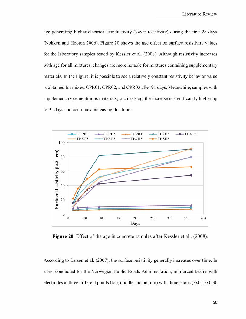
Literature Review
50
age generating higher electrical conductivity (lower resistivity) during the first 28 days
(Nokken and Hooton 2006). Figure 20 shows the age effect on surface resistivity values
for the laboratory samples tested by Kessler et al. (2008). Although resistivity increases
with age for all mixtures, changes are more notable for mixtures containing supplementary
materials. In the Figure, it is possible to see a relatively constant resistivity behavior value
is obtained for mixes, CPR01, CPR02, and CPR03 after 91 days. Meanwhile, samples with
supplementary cementitious materials, such as slag, the increase is significantly higher up
to 91 days and continues increasing this time.
According to Larsen et al. (2007), the surface resistivity generally increases over time. In
a test conducted for the Norwegian Public Roads Administration, reinforced beams with
electrodes at three different points (top, middle and bottom) with dimensions (3x0.15x0.30
0
20
40
60
80
100
0 50 100 150 200 250 300 350 400
Su
rface
Res
isti
vit
y (
kΩ
-cm
)
Days
CPR01 CPR02 CPR03 TB2H5 TB4H5
TB5H5 TB6H5 TB7H5 TB8H5
Figure 20. Effect of the age in concrete samples after Kessler et al., (2008).
Literature Review
51
m) were cast and then submerged half of the beam into sea-water. After 8 months, in June
1998, the beams were removed from this condition and the resistivity was measured using
a frequency of 1000Hz. Later on, in January 2006, 2 days after removal from sea-water the
resistivity was measured at the same three points. Although the season was different, hence
the temperature for the three points, the study concluded that, when the concrete element
is atmospherically exposed, the surface electrical resistivity increased approximately 2.8
times and when the concrete element is submerged, it increased 1.8 times.
2.4.5 Presence of Steel Reinforcing Bars
Electrical measurements in porous materials such as rocks, ceramics and cement
materials can be described as:
𝝆𝑻 = 𝝆𝟎 ∙ 𝟏
𝝋𝜷 [9]
Where 𝜌𝑇 is the total resistivity, 𝜌0 is the resistivity of the pore solution which is function
of the ionic composition and concentration in solution, 𝜑 is the porosity of the system that
is accessible to fluids, and 𝛽 is the connectivity of the pores in the system (Dullien, 1992).
Of course, this law is based on the assumption that the solid skeleton is non-conductive. In
cases where steel reinforcement or steel fibers are used, or when lightweight aggregates
are saturated with a low resistivity solution, it is not validated (Castro et al., 2012; Di Bella
et al., 2012).
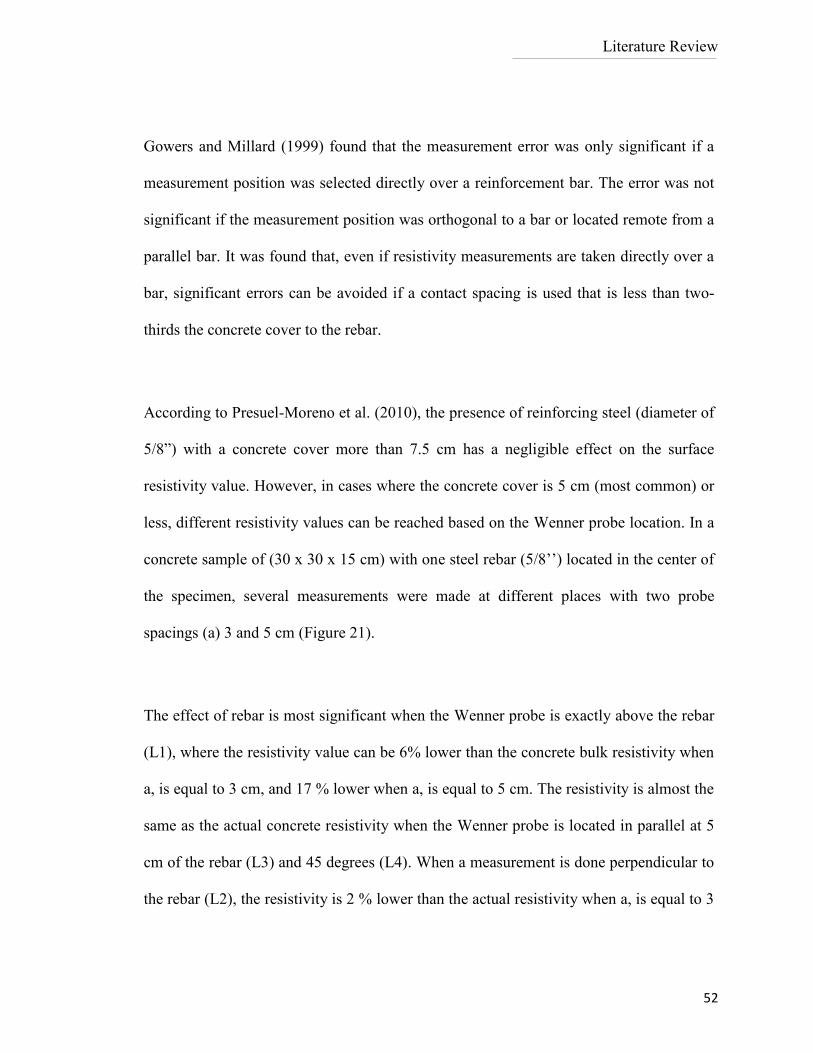
Literature Review
52
Gowers and Millard (1999) found that the measurement error was only significant if a
measurement position was selected directly over a reinforcement bar. The error was not
significant if the measurement position was orthogonal to a bar or located remote from a
parallel bar. It was found that, even if resistivity measurements are taken directly over a
bar, significant errors can be avoided if a contact spacing is used that is less than two-
thirds the concrete cover to the rebar.
According to Presuel-Moreno et al. (2010), the presence of reinforcing steel (diameter of
5/8”) with a concrete cover more than 7.5 cm has a negligible effect on the surface
resistivity value. However, in cases where the concrete cover is 5 cm (most common) or
less, different resistivity values can be reached based on the Wenner probe location. In a
concrete sample of (30 x 30 x 15 cm) with one steel rebar (5/8’’) located in the center of
the specimen, several measurements were made at different places with two probe
spacings (a) 3 and 5 cm (Figure 21).
The effect of rebar is most significant when the Wenner probe is exactly above the rebar
(L1), where the resistivity value can be 6% lower than the concrete bulk resistivity when
a, is equal to 3 cm, and 17 % lower when a, is equal to 5 cm. The resistivity is almost the
same as the actual concrete resistivity when the Wenner probe is located in parallel at 5
cm of the rebar (L3) and 45 degrees (L4). When a measurement is done perpendicular to
the rebar (L2), the resistivity is 2 % lower than the actual resistivity when a, is equal to 3
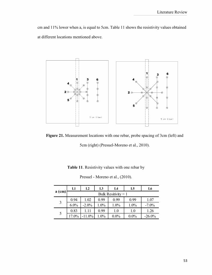
Literature Review
53
cm and 11% lower when a, is equal to 5cm. Table 11 shows the resistivity values obtained
at different locations mentioned above.
L1 L2 L3 L4 L5 L6
0.94 1.02 0.99 0.99 0.99 1.07
6.0% -2.0% 1.0% 1.0% 1.0% -7.0%
0.83 1.11 0.99 1.0 1.0 1.26
17.0% -11.0% 1.0% 0.0% 0.0% -26.0%
3
5
Bulk Resitivity = 1a (cm)
Figure 21. Measurement locations with one rebar, probe spacing of 3cm (left) and
5cm (right) (Presuel-Moreno et al., 2010).
Table 11. Resistivity values with one rebar by
Presuel - Moreno et al., (2010).
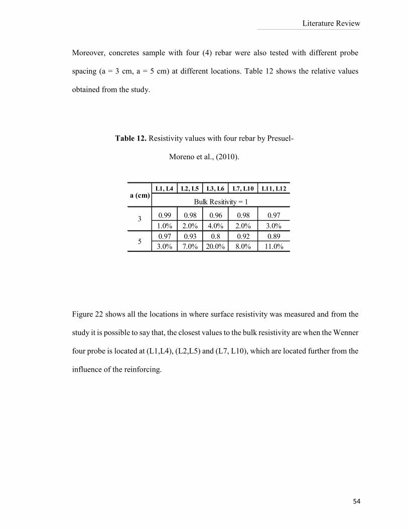
Literature Review
54
Moreover, concretes sample with four (4) rebar were also tested with different probe
spacing (a = 3 cm, a = 5 cm) at different locations. Table 12 shows the relative values
obtained from the study.
Figure 22 shows all the locations in where surface resistivity was measured and from the
study it is possible to say that, the closest values to the bulk resistivity are when the Wenner
four probe is located at (L1,L4), (L2,L5) and (L7, L10), which are located further from the
influence of the reinforcing.
L1, L4 L2, L5 L3, L6 L7, L10 L11, L12
0.99 0.98 0.96 0.98 0.97
1.0% 2.0% 4.0% 2.0% 3.0%
0.97 0.93 0.8 0.92 0.89
3.0% 7.0% 20.0% 8.0% 11.0%
Bulk Resitivity = 1
3
5
a (cm)
Table 12. Resistivity values with four rebar by Presuel-
Moreno et al., (2010).
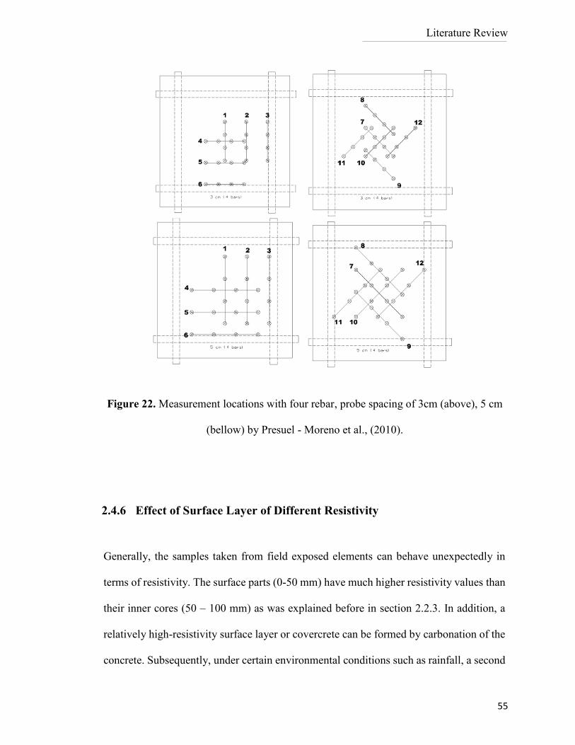
Literature Review
55
Figure 22. Measurement locations with four rebar, probe spacing of 3cm (above), 5 cm
(bellow) by Presuel - Moreno et al., (2010).
2.4.6 Effect of Surface Layer of Different Resistivity
Generally, the samples taken from field exposed elements can behave unexpectedly in
terms of resistivity. The surface parts (0-50 mm) have much higher resistivity values than
their inner cores (50 – 100 mm) as was explained before in section 2.2.3. In addition, a
relatively high-resistivity surface layer or covercrete can be formed by carbonation of the
concrete. Subsequently, under certain environmental conditions such as rainfall, a second
Literature Review
56
low resistivity surface layer will be produced on top of the carbonation layer. However, a
significant error can be avoided if the contact spacing is at least eight times the surface
concrete layer thickness (Gowers and Millard., 1999).
2.4.7 Concrete Non – Homogeneity
The Wenner technique assumes that concrete is homogeneous, but aggregate particles
possess a very high resistivity as was shown in section 2.2.1 (Table 2), and cement paste
has a much lower resistivity. According to Gowers and Millard et al. (1999), from a series
of repetitive measurements it was observed that the standard deviation did not exceed 5%,
as long as the contact spacing was 1.5 times (or greater) as large as the maximum aggregate
size.
2.5 General Factors Influencing Electrical Resistivity due to External
Environment
A report presented by Gowers and Millard et al. (1999) mentioned that, no clear correlation
has been found between the measurement of resistivity and either the ambient relative
humidity of the air or the occurrence of rainfall. The only correlation made so far is for the
temperature, which is inversely proportional to electrical resistivity. According to literature
the parameters as rainfall, moisture and temperature and saturation degree can also
influence resistivity measurements. A detailed explanation of them will be presented next.
Literature Review
57
2.5.1 Rainfall
According to Gowers and Millard (1999), an increase in the measured resistivity using the
Wenner probe technique was observed after rainfall started indicating the double surface
layer effect due to carbonation. One day later, after the concrete surface had dried, the
resistivity measurements returned to their previous values for contact spacing of 𝑎 ≥ 4 cm.
For smaller spacing, this was not the case; for this reason, it is recommended to use a
contact spacing of 𝑎 ≥ 4 cm to minimize the surface wetting effects, even following 24
hours of dry weather.
2.5.2 Moisture Content and Temperature
2.5.2.1 Moisture Content Effect
From literature, it was found that moisture content plays an important role in concrete
resistivity as electrical current in the concrete is carried through interconnected pore water.
Basically, electrical resistivity increases with the decreasing moisture content and usually,
an increase in temperature leads to decrease in resistivity, due to the change in the ion (Na+,
K+, Ca2+, SO42- and OH-) mobility such, ion – ion and ion- solid interactions mobility
(Larsen et al., 2007; Presuel - Moreno et al., 2012; Liu et al., 2014).
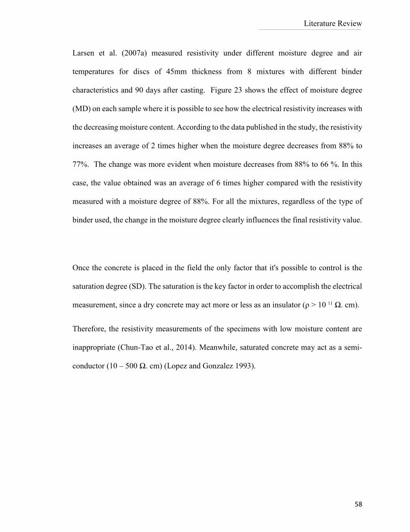
Literature Review
58
Larsen et al. (2007a) measured resistivity under different moisture degree and air
temperatures for discs of 45mm thickness from 8 mixtures with different binder
characteristics and 90 days after casting. Figure 23 shows the effect of moisture degree
(MD) on each sample where it is possible to see how the electrical resistivity increases with
the decreasing moisture content. According to the data published in the study, the resistivity
increases an average of 2 times higher when the moisture degree decreases from 88% to
77%. The change was more evident when moisture decreases from 88% to 66 %. In this
case, the value obtained was an average of 6 times higher compared with the resistivity
measured with a moisture degree of 88%. For all the mixtures, regardless of the type of
binder used, the change in the moisture degree clearly influences the final resistivity value.
Once the concrete is placed in the field the only factor that it's possible to control is the
saturation degree (SD). The saturation is the key factor in order to accomplish the electrical
measurement, since a dry concrete may act more or less as an insulator (ρ > 10 11 Ω. cm).
Therefore, the resistivity measurements of the specimens with low moisture content are
inappropriate (Chun-Tao et al., 2014). Meanwhile, saturated concrete may act as a semi-
conductor (10 – 500 Ω. cm) (Lopez and Gonzalez 1993).
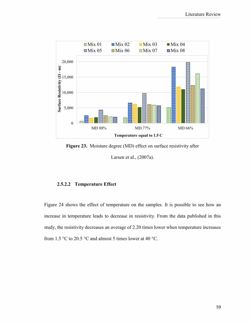
Literature Review
59
2.5.2.2 Temperature Effect
Figure 24 shows the effect of temperature on the samples. It is possible to see how an
increase in temperature leads to decrease in resistivity. From the data published in this
study, the resistivity decreases an average of 2.20 times lower when temperature increases
from 1.5 °C to 20.5 °C and almost 5 times lower at 40 °C.
0
5,000
10,000
15,000
20,000
MD 88% MD 77% MD 66%
Su
rfa
ce R
esis
tiv
ity
(Ω
-m
)
Temperature equal to 1.5 C
Mix 01 Mix 02 Mix 03 Mix 04
Mix 05 Mix 06 Mix 07 Mix 08
Figure 23. Moisture degree (MD) effect on surface resistivity after
Larsen et al., (2007a).
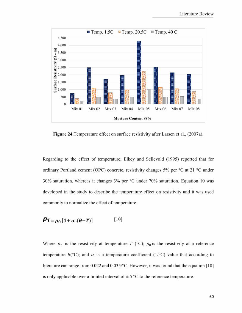
Literature Review
60
Figure 24.Temperature effect on surface resistivity after Larsen et al., (2007a).
Regarding to the effect of temperature, Elkey and Sellevold (1995) reported that for
ordinary Portland cement (OPC) concrete, resistivity changes 5% per °C at 21 °C under
30% saturation, whereas it changes 3% per °C under 70% saturation. Equation 10 was
developed in the study to describe the temperature effect on resistivity and it was used
commonly to normalize the effect of temperature.
𝝆𝑻= 𝝆𝟎 [𝟏+ 𝜶 .(𝜽−𝑻)] [10]
Where 𝜌𝑇 is the resistivity at temperature 𝑇 (°C); 𝜌0 is the resistivity at a reference
temperature 𝜃(°C); and 𝛼 is a temperature coefficient (1/°C) value that according to
literature can range from 0.022 and 0.035/°C. However, it was found that the equation [10]
is only applicable over a limited interval of ± 5 °C to the reference temperature.
0
500
1,000
1,500
2,000
2,500
3,000
3,500
4,000
4,500
Mix 01 Mix 02 Mix 03 Mix 04 Mix 05 Mix 06 Mix 07 Mix 08
Su
rfa
ce R
esis
tiv
ity
(Ω
-m
)
Mosture Content 88%
Temp. 1.5C Temp. 20.5C Temp. 40 C
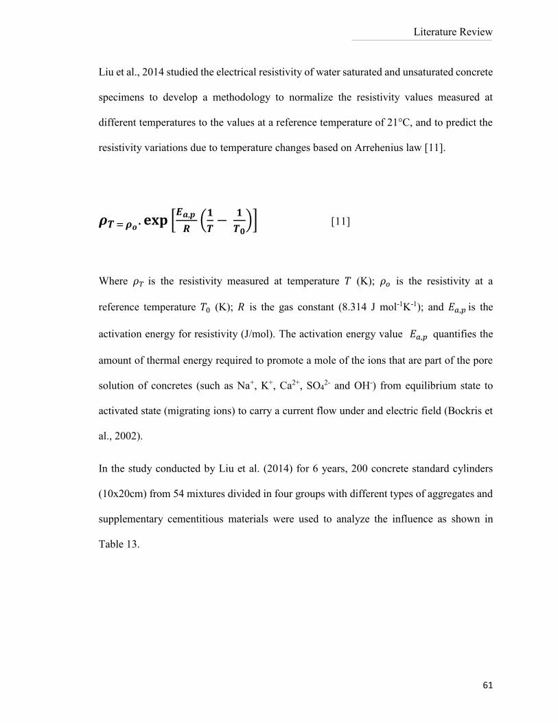
Literature Review
61
Liu et al., 2014 studied the electrical resistivity of water saturated and unsaturated concrete
specimens to develop a methodology to normalize the resistivity values measured at
different temperatures to the values at a reference temperature of 21°C, and to predict the
resistivity variations due to temperature changes based on Arrehenius law [11].
𝝆𝑻 = 𝝆𝒐. 𝐞𝐱𝐩 [
𝑬𝒂,𝒑
𝑹(
𝟏
𝑻−
𝟏
𝑻𝟎)] [11]
Where 𝜌𝑇 is the resistivity measured at temperature 𝑇 (K); 𝜌𝑜 is the resistivity at a
reference temperature 𝑇0 (K); 𝑅 is the gas constant (8.314 J mol-1K-1); and 𝐸𝑎,𝑝 is the
activation energy for resistivity (J/mol). The activation energy value 𝐸𝑎,𝑝 quantifies the
amount of thermal energy required to promote a mole of the ions that are part of the pore
solution of concretes (such as Na+, K+, Ca2+, SO42- and OH-) from equilibrium state to
activated state (migrating ions) to carry a current flow under and electric field (Bockris et
al., 2002).
In the study conducted by Liu et al. (2014) for 6 years, 200 concrete standard cylinders
(10x20cm) from 54 mixtures divided in four groups with different types of aggregates and
supplementary cementitious materials were used to analyze the influence as shown in
Table 13.
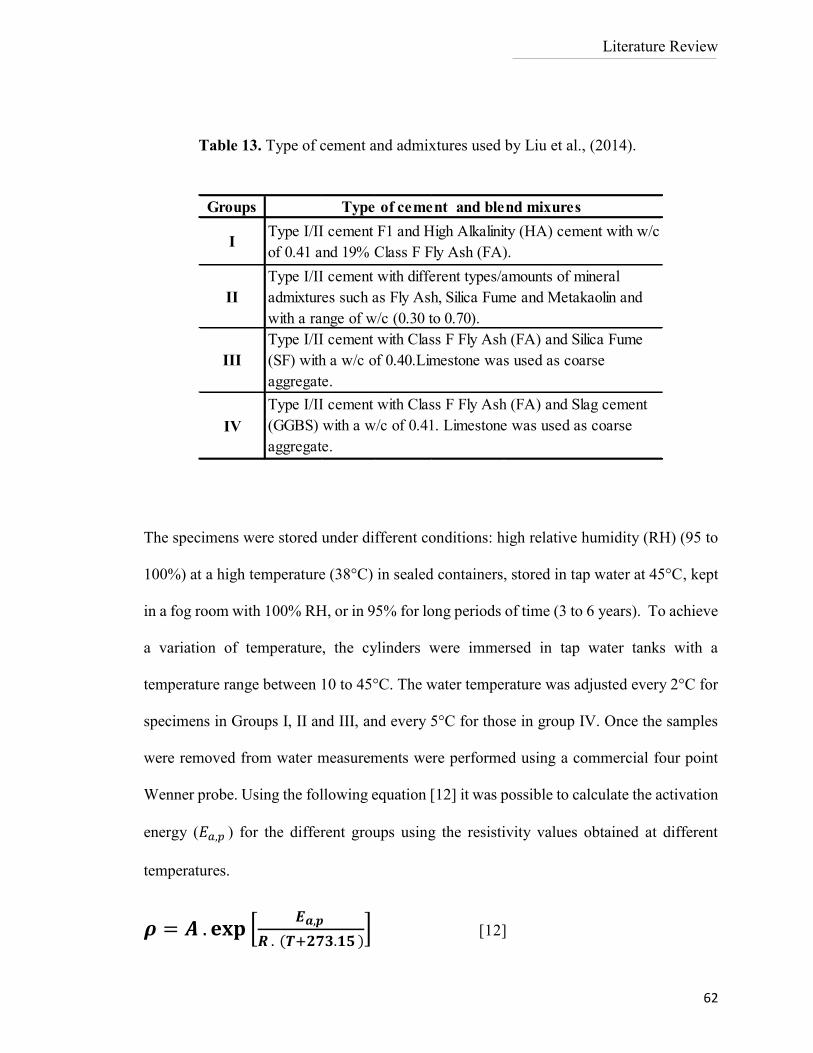
Literature Review
62
The specimens were stored under different conditions: high relative humidity (RH) (95 to
100%) at a high temperature (38°C) in sealed containers, stored in tap water at 45°C, kept
in a fog room with 100% RH, or in 95% for long periods of time (3 to 6 years). To achieve
a variation of temperature, the cylinders were immersed in tap water tanks with a
temperature range between 10 to 45°C. The water temperature was adjusted every 2°C for
specimens in Groups I, II and III, and every 5°C for those in group IV. Once the samples
were removed from water measurements were performed using a commercial four point
Wenner probe. Using the following equation [12] it was possible to calculate the activation
energy (𝐸𝑎,𝑝 ) for the different groups using the resistivity values obtained at different
temperatures.
𝝆 = 𝑨 . 𝐞𝐱𝐩 [𝑬𝒂,𝒑
𝑹 . (𝑻+𝟐𝟕𝟑.𝟏𝟓 )] [12]
Groups
III
Type I/II cement with Class F Fly Ash (FA) and Silica Fume
(SF) with a w/c of 0.40.Limestone was used as coarse
aggregate.
Type I/II cement with Class F Fly Ash (FA) and Slag cement
(GGBS) with a w/c of 0.41. Limestone was used as coarse
aggregate.
IV
Type of cement and blend mixures
Type I/II cement F1 and High Alkalinity (HA) cement with w/c
of 0.41 and 19% Class F Fly Ash (FA).I
Type I/II cement with different types/amounts of mineral
admixtures such as Fly Ash, Silica Fume and Metakaolin and
with a range of w/c (0.30 to 0.70).
II
Table 13. Type of cement and admixtures used by Liu et al., (2014).
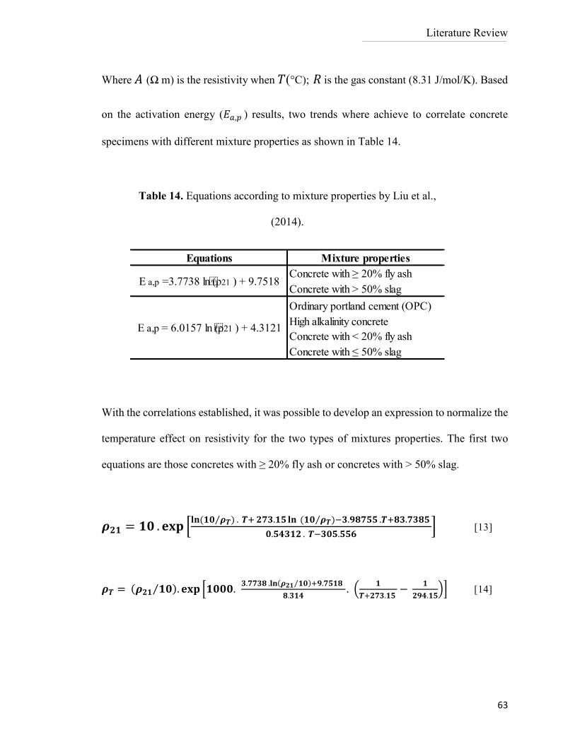
Literature Review
63
Where 𝐴 (Ω m) is the resistivity when 𝑇(°C); 𝑅 is the gas constant (8.31 J/mol/K). Based
on the activation energy (𝐸𝑎,𝑝 ) results, two trends where achieve to correlate concrete
specimens with different mixture properties as shown in Table 14.
With the correlations established, it was possible to develop an expression to normalize the
temperature effect on resistivity for the two types of mixtures properties. The first two
equations are those concretes with ≥ 20% fly ash or concretes with > 50% slag.
𝝆𝟐𝟏 = 𝟏𝟎 . 𝐞𝐱𝐩 [𝐥𝐧(𝟏𝟎 𝝆𝑻) . 𝑻+ 𝟐𝟕𝟑.𝟏𝟓 𝐥𝐧 (𝟏𝟎 𝝆𝑻)−𝟑.𝟗𝟖𝟕𝟓𝟓 .𝑻+𝟖𝟑.𝟕𝟑𝟖𝟓 ⁄⁄
𝟎.𝟓𝟒𝟑𝟏𝟐 . 𝑻−𝟑𝟎𝟓.𝟓𝟓𝟔] [13]
𝝆𝑻 = (𝝆𝟐𝟏 𝟏𝟎⁄ ). 𝐞𝐱𝐩 [𝟏𝟎𝟎𝟎. 𝟑.𝟕𝟕𝟑𝟖 .𝐥𝐧(𝝆𝟐𝟏 𝟏𝟎⁄ )+𝟗.𝟕𝟓𝟏𝟖
𝟖.𝟑𝟏𝟒. (
𝟏
𝑻+𝟐𝟕𝟑.𝟏𝟓 −
𝟏
𝟐𝟗𝟒.𝟏𝟓)] [14]
Equations Mixture properties
Concrete with ≥ 20% fly ash
Concrete with > 50% slag
Ordinary portland cement (OPC)
High alkalinity concrete
Concrete with < 20% fly ash
Concrete with ≤ 50% slag
E a,p =3.7738 ln (ρ21 ) + 9.7518
E a,p = 6.0157 ln (ρ21 ) + 4.3121
Table 14. Equations according to mixture properties by Liu et al.,
(2014).
Literature Review
64
The second set of equations are for those concretes with only ordinary Portland cement
(OPC), high alkalinity, concretes with < 20% fly ash, concretes with ≤ 50% slag ≥ 20% fly
ash or concretes with > 50% slag.
𝝆𝟐𝟏 = 𝟏𝟎 . 𝐞𝐱𝐩 [𝐥𝐧(𝟏𝟎 𝝆𝑻) . 𝑻+ 𝟐𝟕𝟑.𝟏𝟓 𝐥𝐧 (𝟏𝟎 𝝆𝑻)−𝟏.𝟕𝟔𝟒𝟎𝟓 .𝑻+𝟑𝟕.𝟎𝟒𝟓 ⁄⁄
𝟏.𝟒𝟓𝟗𝟖𝟓 . 𝑻−𝟑𝟐𝟒.𝟖𝟎𝟖] [15]
𝝆𝑻 = (𝝆𝟐𝟏 𝟏𝟎⁄ ). 𝐞𝐱𝐩 [𝟏𝟎𝟎𝟎. 𝟔.𝟎𝟏𝟓𝟕 .𝐥𝐧(𝝆𝟐𝟏 𝟏𝟎⁄ )+𝟒.𝟑𝟏𝟐𝟏
𝟖.𝟑𝟏𝟒. (
𝟏
𝑻+𝟐𝟕𝟑.𝟏𝟓 −
𝟏
𝟐𝟗𝟒.𝟏𝟓)] [16]
Where 𝜌𝑇 (Ω m) is the measured resistivity at temperature 𝑇(°C). Then is necessary to
calculate 𝜌21(reference resistivity at 21°C) by plugging 𝜌𝑇 and 𝑇 into equations [13] or
[15] according to the case to finally calculate resistivity at other temperatures by plugging
𝜌21 into equations [14] or [16] according the case. However, this methodology does not
take into account the effect generated by moisture content an additional factor that can
influence resistivity values. These temperature correlations were established using only
standard cylinders specimen samples (Ø10x20cm).
2.5.3 Saturation Degree (SD)
Once the concrete is placed in the field the only factor that it's possible to control is the
saturation degree. The saturation is the key factor in order to accomplish the electrical
Literature Review
65
measurement, since a dry concrete may act more or less as an insulator (ρ > 10 11 Ω. cm).
Therefore, the resistivity measurements of the specimens with low moisture content are
inappropriate (Chun-Tao et al., 2014). Meanwhile, saturated concrete may act as a semi-
conductor (10 – 500 Ω. cm) (Lopez and Gonzolez 1993).
A characteristic example of saturation on a concrete bridge deck can be seen in Figure 25.
It can be noticed that the duration of saturation is very brief; a) Several points have been
measured (showing damp) and points that are going to be measured (paint dots) using the
Wenner four probe device; b) Close view of the Wenner probe device over the concrete
element; c) Another none destructive test (NDT) device called galvanostatic pulse
measurement (GPM) used to measure corrosion rates over ponding saturate surface; d) An
unreliable surface resistivity value is showed over a concrete element without saturation.
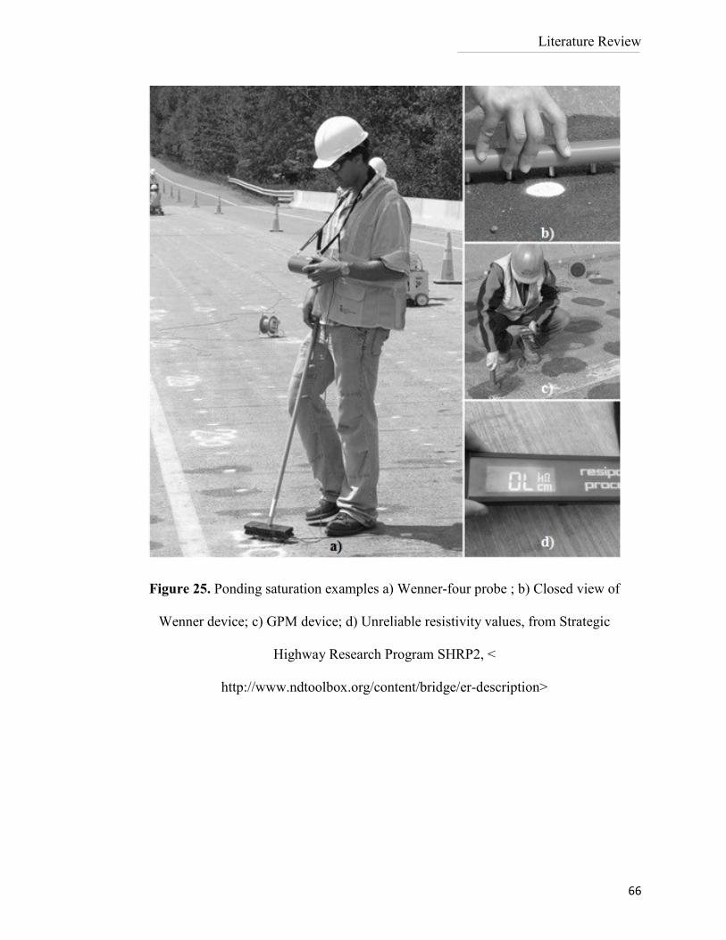
Literature Review
66
Figure 25. Ponding saturation examples a) Wenner-four probe ; b) Closed view of
Wenner device; c) GPM device; d) Unreliable resistivity values, from Strategic
Highway Research Program SHRP2, <
http://www.ndtoolbox.org/content/bridge/er-description>
67
3 Laboratory and Work Practice Methodology
The objective of this work is to investigate issues involved in advancing the use of surface
resistivity in the field. The development of a test method suitable for non-destructive field
use to evaluate the potential durability of the surface layer or covercrete by determining
the surface electrical resistivity would be a useful test. The following phases were
established to analyze their influence on surface electrical resistivity:
Phase One – Influence of Saturation Degree.
Phase Two – Influence of Sample Storage under Different Solutions and
Specimen Geometry.
Phase Three – Analyses of Correlations to Normalize Temperature Effect on Site
and influence of Curved and Plane Surfaces.
Phase Four – Influence of Saturation Methods Techniques.
The phase one, two and four were completed under laboratory conditions at Concordia
University. Phase Three was carried out at Concordia University, at University of
Sherbrooke and directly on field over sidewalks cast for the City of Montreal (Ville de
Montréal) located at North - East of Montreal, QC. Canada.
Laboratory and Work Practice Methodology
68
3.1 Phase One – Influence of Saturation Duration
Five binder combinations were investigated in this portion of the work in order to represent
a wide variety of concretes from high performance to residential concretes; all but one of
these combinations included the use of blast furnace slag. Rupnow and Icenogle et al.,
(2011) found that in concrete mixtures with slag, increasing of w/c gave increasing
resistivity. As mentioned in the literature review, decreasing porosity achieved with lower
water to cement ratios should lead to increased resistivity. Therefore, the laboratory
mixtures for this phase are focused on mixtures containing slag in order to validate this
behavior.
Table 15 shows the laboratory mixture designs used as well as fresh and hardened
properties. Type I/II Portland (TI) and Portland-limestone (L) cement were used as the
primary binders. The supplementary cementitious materials used were Grade 100 blast
furnace slag (S) and Type F fly ash (F). Aggregates consisted of 14 mm coarse aggregate
and natural sand. For each binder combination, five mixtures were made with w/c ranging
from 0.32 to 0.64.
Chemical admixtures included air entrainer and water reducers were used to achieve target
air of 5.0% and slump of 100 ± 10 mm. Slump and entrained air were measured at the
time of casting using ASTM methods ASTM C1611 / C1611M - 14 (2014) and ASTM
test C - 666 (2008) procedures A and B. As well, compressive strength was measured as
the average of two cylinders using ASTM C39 / C39M - 14a (2014) at 56 days as is typical
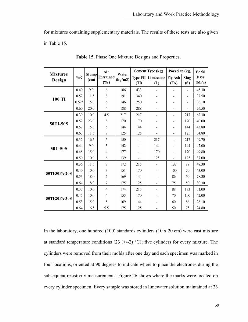
Laboratory and Work Practice Methodology
69
for mixtures containing supplementary materials. The results of these tests are also given
in Table 15.
In the laboratory, one hundred (100) standards cylinders (10 x 20 cm) were cast mixture
at standard temperature conditions (23 (+/-2) °C); five cylinders for every mixture. The
cylinders were removed from their molds after one day and each specimen was marked in
four locations, oriented at 90 degrees to indicate where to place the electrodes during the
subsequent resistivity measurements. Figure 26 shows where the marks were located on
every cylinder specimen. Every sample was stored in limewater solution maintained at 23
Table 15. Phase One Mixture Designs and Properties.
0.40 9.0 6 186 433 - - - 45.30
0.52 11.5 8 191 340 - - - 37.50
0.52* 15.0 6 146 250 - - - 36.10
0.60 20.0 4 188 288 - - - 26.50
0.39 10.0 4.5 217 217 - - 217 62.30
0.52 23.0 8 170 170 - - 170 40.00
0.57 15.0 5 144 144 - - 144 43.80
0.63 11.5 7 125 125 - - 125 34.80
0.32 16.5 5 150 - 217 - 217 49.70
0.44 9.0 5 142 - 144 - 144 47.00
0.48 15.0 4 177 - 170 - 170 49.80
0.50 10.0 6 139 - 125 - 125 37.00
0.36 11.5 7 172 215 - 133 88 48.30
0.40 10.0 3 151 170 - 100 70 43.00
0.53 18.0 5 169 144 - 86 60 28.30
0.64 18.0 7 175 125 - 75 50 30.30
0.37 10.0 4 174 215 - 88 133 51.00
0.45 10.0 4 155 170 - 70 100 42.00
0.53 15.0 5 169 144 - 60 86 28.10
0.64 16.5 5.5 175 125 - 50 75 24.80
Pozzolan (kg) f'c 56
Days
(MPa)
Type I/II
(TI)
Limestone
(L)
Fly Ash
(FA)
Slag
(S)
100 TI
50TI-50S
50L-50S
50TI-30FA-20S
50TI-20FA-30S
Mixtures
Designw/c
Slump
(cm)
Air
Entrained
(% )
Water
(kg/m3)
Cement Type (kg)
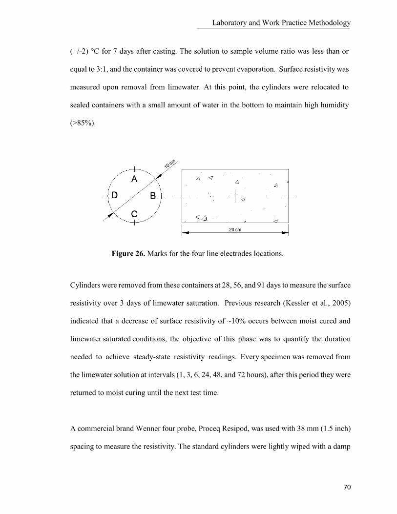
Laboratory and Work Practice Methodology
70
(+/-2) °C for 7 days after casting. The solution to sample volume ratio was less than or
equal to 3:1, and the container was covered to prevent evaporation. Surface resistivity was
measured upon removal from limewater. At this point, the cylinders were relocated to
sealed containers with a small amount of water in the bottom to maintain high humidity
(>85%).
Cylinders were removed from these containers at 28, 56, and 91 days to measure the surface
resistivity over 3 days of limewater saturation. Previous research (Kessler et al., 2005)
indicated that a decrease of surface resistivity of ~10% occurs between moist cured and
limewater saturated conditions, the objective of this phase was to quantify the duration
needed to achieve steady-state resistivity readings. Every specimen was removed from
the limewater solution at intervals (1, 3, 6, 24, 48, and 72 hours), after this period they were
returned to moist curing until the next test time.
A commercial brand Wenner four probe, Proceq Resipod, was used with 38 mm (1.5 inch)
spacing to measure the resistivity. The standard cylinders were lightly wiped with a damp
Figure 26. Marks for the four line electrodes locations.
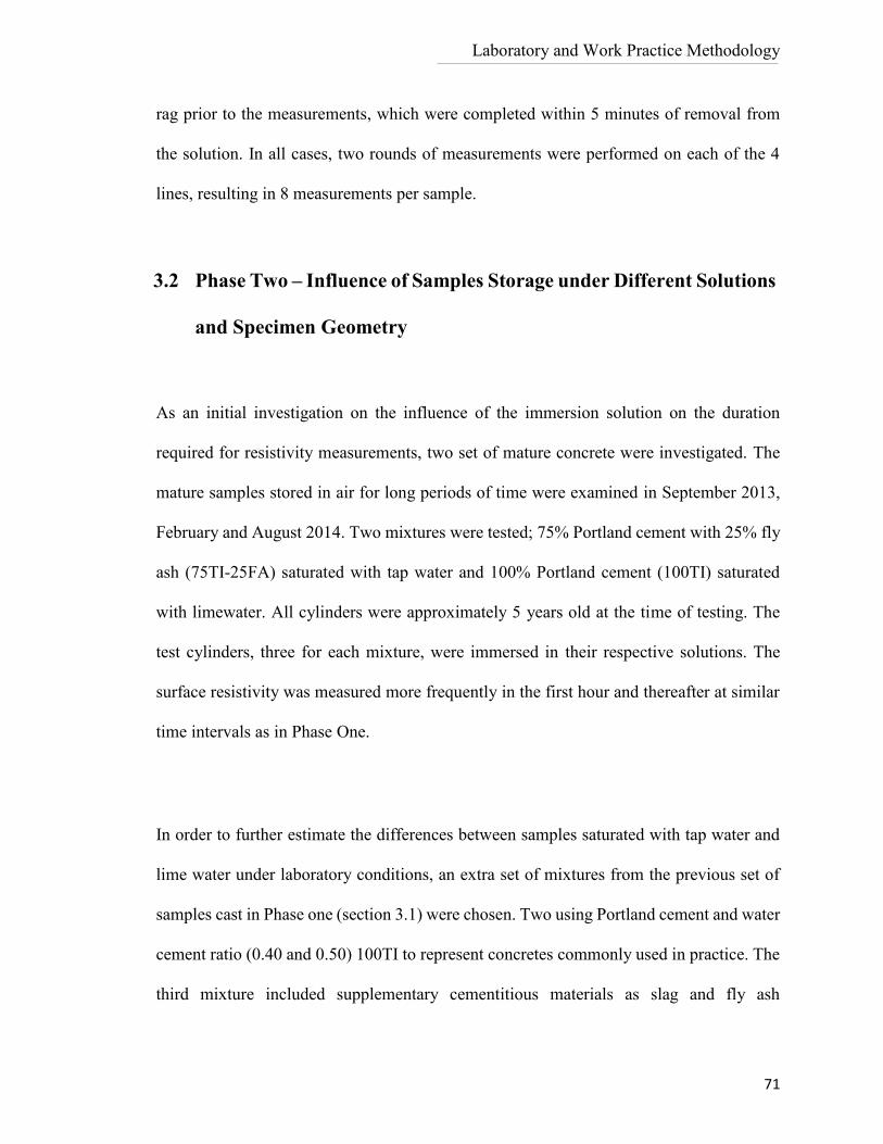
Laboratory and Work Practice Methodology
71
rag prior to the measurements, which were completed within 5 minutes of removal from
the solution. In all cases, two rounds of measurements were performed on each of the 4
lines, resulting in 8 measurements per sample.
3.2 Phase Two – Influence of Samples Storage under Different Solutions
and Specimen Geometry
As an initial investigation on the influence of the immersion solution on the duration
required for resistivity measurements, two set of mature concrete were investigated. The
mature samples stored in air for long periods of time were examined in September 2013,
February and August 2014. Two mixtures were tested; 75% Portland cement with 25% fly
ash (75TI-25FA) saturated with tap water and 100% Portland cement (100TI) saturated
with limewater. All cylinders were approximately 5 years old at the time of testing. The
test cylinders, three for each mixture, were immersed in their respective solutions. The
surface resistivity was measured more frequently in the first hour and thereafter at similar
time intervals as in Phase One.
In order to further estimate the differences between samples saturated with tap water and
lime water under laboratory conditions, an extra set of mixtures from the previous set of
samples cast in Phase one (section 3.1) were chosen. Two using Portland cement and water
cement ratio (0.40 and 0.50) 100TI to represent concretes commonly used in practice. The
third mixture included supplementary cementitious materials as slag and fly ash
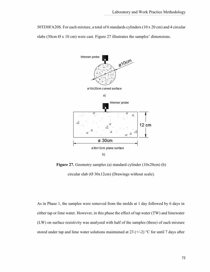
Laboratory and Work Practice Methodology
72
50TI30FA20S. For each mixture, a total of 6 standards cylinders (10 x 20 cm) and 4 circular
slabs (30cm Ø x 10 cm) were cast. Figure 27 illustrates the samples’ dimensions.
As in Phase 1, the samples were removed from the molds at 1 day followed by 6 days in
either tap or lime water. However, in this phase the effect of tap water (TW) and limewater
(LW) on surface resistivity was analyzed with half of the samples (three) of each mixture
stored under tap and lime water solutions maintained at 23 (+/-2) °C for until 7 days after
Figure 27. Geometry samples (a) standard cylinder (10x20cm) (b)
circular slab (Ø 30x12cm) (Drawings without scale).
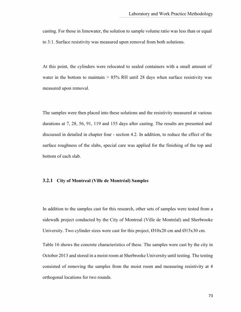
Laboratory and Work Practice Methodology
73
casting. For those in limewater, the solution to sample volume ratio was less than or equal
to 3:1. Surface resistivity was measured upon removal from both solutions.
At this point, the cylinders were relocated to sealed containers with a small amount of
water in the bottom to maintain > 85% RH until 28 days when surface resistivity was
measured upon removal.
The samples were then placed into these solutions and the resistivity measured at various
durations at 7, 28, 56, 91, 119 and 155 days after casting. The results are presented and
discussed in detailed in chapter four - section 4.2. In addition, to reduce the effect of the
surface roughness of the slabs, special care was applied for the finishing of the top and
bottom of each slab.
3.2.1 City of Montreal (Ville de Montréal) Samples
In addition to the samples cast for this research, other sets of samples were tested from a
sidewalk project conducted by the City of Montreal (Ville de Montréal) and Sherbrooke
University. Two cylinder sizes were cast for this project, Ø10x20 cm and Ø15x30 cm.
Table 16 shows the concrete characteristics of these. The samples were cast by the city in
October 2013 and stored in a moist room at Sherbrooke University until testing. The testing
consisted of removing the samples from the moist room and measuring resistivity at 4
orthogonal locations for two rounds.
Laboratory and Work Practice Methodology
74
3.3 Phase Three – Analysis of Correlations to Normalize Temperature
Effect on Site and the Influence of Curved and Plane Surfaces
The motivation in this section was to evaluate the correlations established by Liu et al.,
(2014) to normalize temperature effects for resistivity measured directly on site. The
objective was to verify if it was possible to achieve a singular or very close resistivity
value after applying the equations 15 and 16 developed by the study. The on-site resistivity
was also compared to that of the lab specimens conducted at nearly the same age.
Mixture General information
73% GU, 27% GUb-SF(silica fume blended Portland
cement), w/c 0.43, max. agg. size 20 mmVdeMTL Temoin
75% GU, 25% glass powder , w/c 0.40, max. agg.
size 20 mm
90% GU, 10% glass powder , w/c 0.41, max. agg.
size 20 mm
VdeMTL 25PV
VdeMTL 10PV
Table 16. Concrete mixtures by city of Montreal
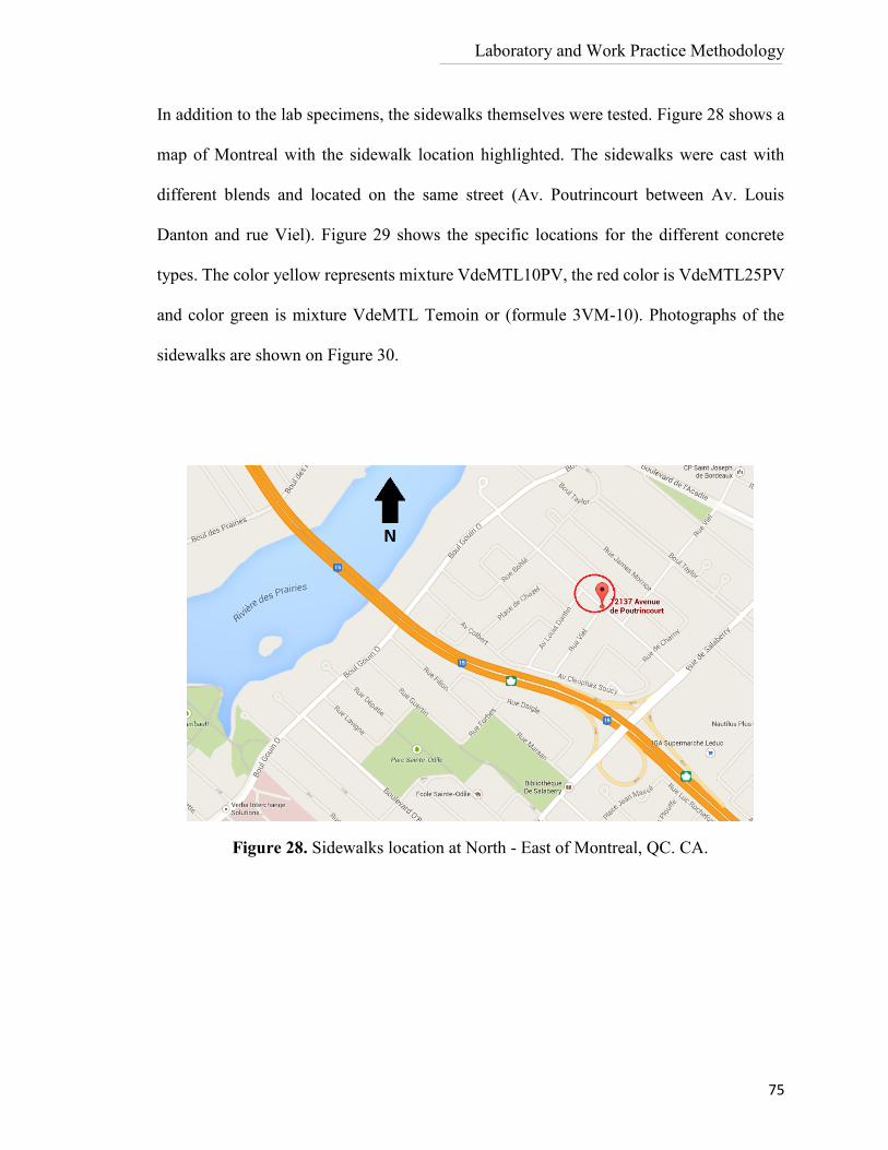
Laboratory and Work Practice Methodology
75
In addition to the lab specimens, the sidewalks themselves were tested. Figure 28 shows a
map of Montreal with the sidewalk location highlighted. The sidewalks were cast with
different blends and located on the same street (Av. Poutrincourt between Av. Louis
Danton and rue Viel). Figure 29 shows the specific locations for the different concrete
types. The color yellow represents mixture VdeMTL10PV, the red color is VdeMTL25PV
and color green is mixture VdeMTL Temoin or (formule 3VM-10). Photographs of the
sidewalks are shown on Figure 30.
Figure 28. Sidewalks location at North - East of Montreal, QC. CA.
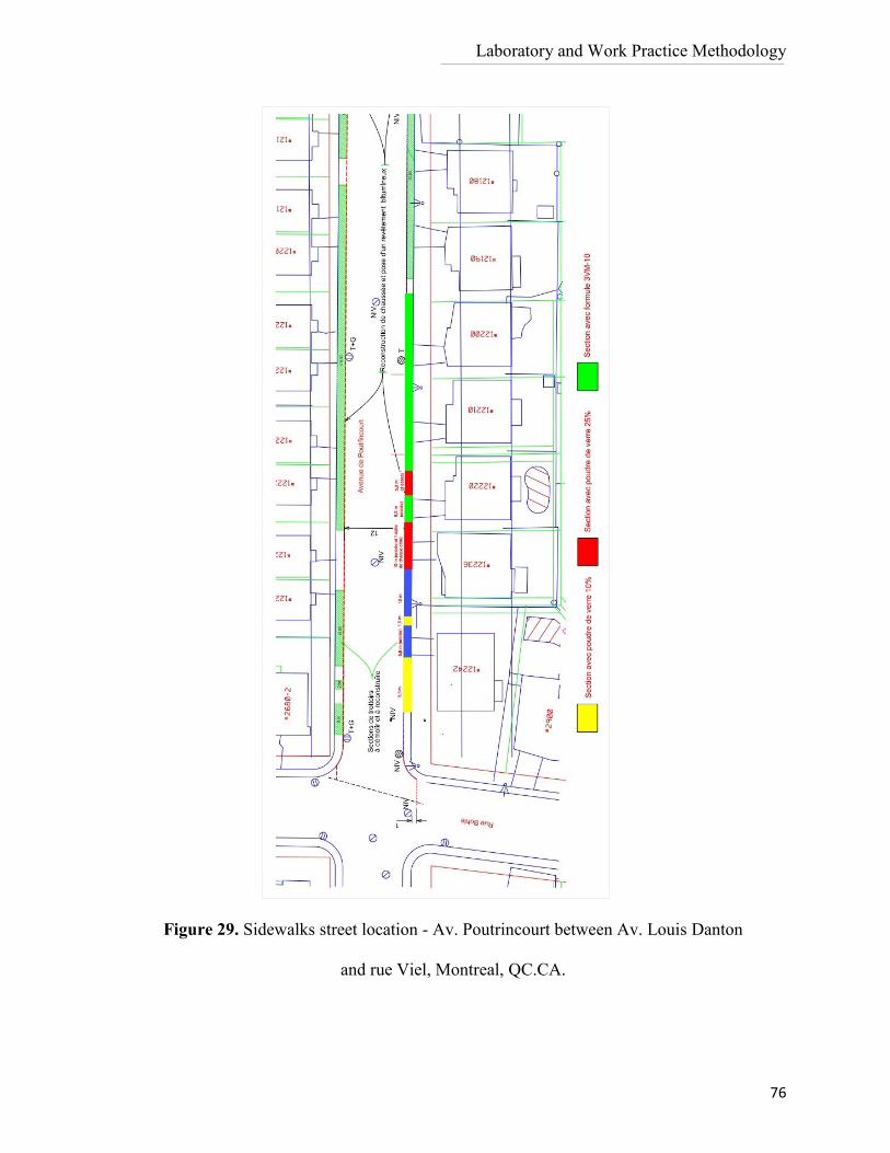
Laboratory and Work Practice Methodology
76
Figure 29. Sidewalks street location - Av. Poutrincourt between Av. Louis Danton
and rue Viel, Montreal, QC.CA.
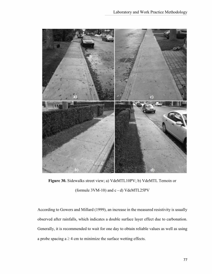
Laboratory and Work Practice Methodology
77
According to Gowers and Millard (1999), an increase in the measured resistivity is usually
observed after rainfalls, which indicates a double surface layer effect due to carbonation.
Generally, it is recommended to wait for one day to obtain reliable values as well as using
a probe spacing a ≥ 4 cm to minimize the surface wetting effects.
Figure 30. Sidewalks street view; a) VdeMTL10PV; b) VdeMTL Temoin or
(formule 3VM-10) and c - d) VdeMTL25PV
Laboratory and Work Practice Methodology
78
On each sidewalk, no evidence of carbonation was observed. Each measurement started
after one hour the rain was over, until the excess of water had evaporated, but the sidewalk
was still significantly wet. A total of 16 measurements per mixture were conducted directly
on the sidewalks after rainfalls during two different days (September 11 and 13, 2014). The
average rain precipitation was registered as 5-10 mm for both days.
The average concrete temperatures registered during these days were 10.5 and 15,
respectively using a handheld infrared thermometer. The probe spacing used was equal to
38.1mm (1.5in).
Each measurement started after one hour the rain was over, until the excess of water was
evaporated in order to keep the area moisture. The average rain precipitation was registered
as (5-10 mm). The average concrete temperatures registered during these days were (10.5
and 15). The probe spacing used was equal to 38.1mm (1.5in).
Additionally, a comparison was established between the data obtained on field over the
sidewalk, representing plane surfaces and the resistivity measured over the standard
cylinders Ø10x20cm and Ø15x30cm, curved surfaces cast for the City of Montreal project
described before in Section 3.2.1.
3.4 Phase Four – Influence of Saturation Methods Techniques
The motivation of this section was to establish a relation between different types of
saturation methods used or alternatives that can be used on site to reach a similar degree
of saturation found in laboratory conditions to obtain reliable surface resistivity values.
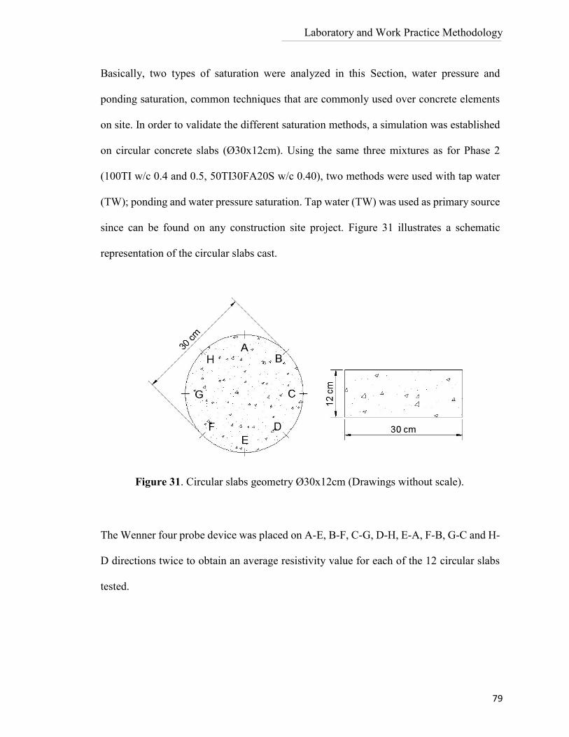
Laboratory and Work Practice Methodology
79
Basically, two types of saturation were analyzed in this Section, water pressure and
ponding saturation, common techniques that are commonly used over concrete elements
on site. In order to validate the different saturation methods, a simulation was established
on circular concrete slabs (Ø30x12cm). Using the same three mixtures as for Phase 2
(100TI w/c 0.4 and 0.5, 50TI30FA20S w/c 0.40), two methods were used with tap water
(TW); ponding and water pressure saturation. Tap water (TW) was used as primary source
since can be found on any construction site project. Figure 31 illustrates a schematic
representation of the circular slabs cast.
The Wenner four probe device was placed on A-E, B-F, C-G, D-H, E-A, F-B, G-C and H-
D directions twice to obtain an average resistivity value for each of the 12 circular slabs
tested.
Figure 31. Circular slabs geometry Ø30x12cm (Drawings without scale).
Laboratory and Work Practice Methodology
80
3.4.1 Water Pressure Saturation
To determine influence of water pressure on surface electrical resistivity at 125 days of
casting, the same circular slabs Ø30x12cm samples described previously in Section 3.2
were tested after using a commercial water pressure machine - archer K3.690 in order to
simulate a common practice on site to saturate concretes in a short period of time.
A total of four rounds of resistivity measurements were made at different times: after 10,
20, 30 and 40 minutes of continuous water exposure.
3.4.2 Ponding Saturation
To establish a comparison between the effect of fully immersed samples and ponding
saturation, samples were saturated by surface ponding with tap water simulating common
field practices.
A total of 12 circular slab samples Ø30x12cm were stored in air and tested at 205 days
under laboratory conditions in order to achieve a relatively dry element. Then, for periods
of time (10, 30 and 60 minutes), the samples were surface saturated (by ponding) to
simulate a potential on site saturation practice. After this, they were immersed in tap-water
until a constant resistivity value was achieved. Figure 32 shows a circular slab Ø30x12cm
with 12.5 mm neoprene gasket on the edge to simulate ponding saturation.
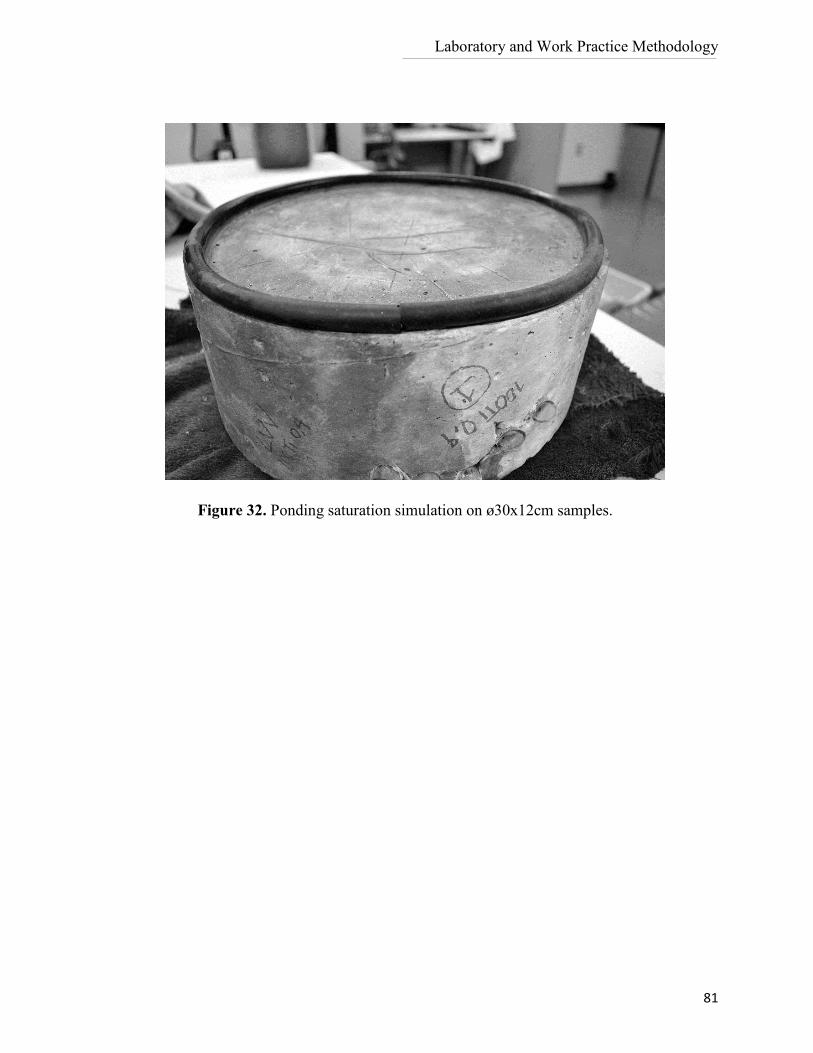
Laboratory and Work Practice Methodology
81
Figure 32. Ponding saturation simulation on ø30x12cm samples.
82
4 Results of Phases
The following pages contain the results obtained for each phase; several comparisons were
established in order to understand and analyze the influence of surface electrical resistivity
when is influenced of several factors under laboratory and field conditions.
4.1 Phase One - Influence of Saturation Degree
For this part, the influence of saturation duration and its tendency at different ages (28, 56
and 91 days) was analyzed on five binder systems. All the electrical resistivity results
presented include the correction geometry factor using equation [6] from section 2.3.2 and
all the measurements were made with the same probe spacing, 𝑎 = 3.81 𝑐𝑚. As mentioned
before, for the standard cylinders (10 x 20cm) the correction factor is 1.887. The results
presented here are therefore 1.887 lower than measured.
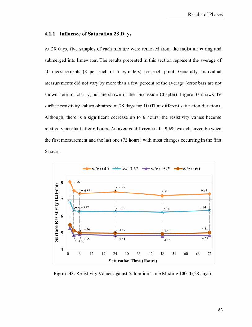
Results of Phases
83
4.1.1 Influence of Saturation 28 Days
At 28 days, five samples of each mixture were removed from the moist air curing and
submerged into limewater. The results presented in this section represent the average of
40 measurements (8 per each of 5 cylinders) for each point. Generally, individual
measurements did not vary by more than a few percent of the average (error bars are not
shown here for clarity, but are shown in the Discussion Chapter). Figure 33 shows the
surface resistivity values obtained at 28 days for 100TI at different saturation durations.
Although, there is a significant decrease up to 6 hours; the resistivity values become
relatively constant after 6 hours. An average difference of - 9.6% was observed between
the first measurement and the last one (72 hours) with most changes occurring in the first
6 hours.
Figure 33. Resistivity Values against Saturation Time Mixture 100TI (28 days).
7.56
6.866.97
6.73 6.84
5.845.77 5.78 5.745.84
4.354.38 4.34 4.32
4.35
4.50 4.47 4.444.51
4
5
6
7
8
0 6 12 18 24 30 36 42 48 54 60 66 72
Su
rface
Res
isti
vit
y (
kΩ
-cm
)
Saturation Time (Hours)
w/c 0.40 w/c 0.52 w/c 0.52* w/c 0.60
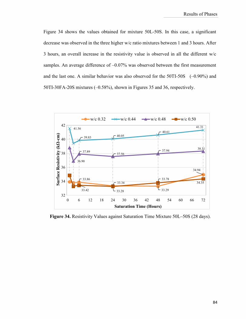
Results of Phases
84
Figure 34 shows the values obtained for mixture 50L-50S. In this case, a significant
decrease was observed in the three higher w/c ratio mixtures between 1 and 3 hours. After
3 hours, an overall increase in the resistivity value is observed in all the different w/c
samples. An average difference of –0.07% was observed between the first measurement
and the last one. A similar behavior was also observed for the 50TI-50S (–0.90%) and
50TI-30FA-20S mixtures (–0.58%), shown in Figures 35 and 36, respectively.
Figure 34. Resistivity Values against Saturation Time Mixture 50L–50S (28 days).
33.8633.34
33.29
34.94
41.56
39.8340.05
40.61
41.31
36.90
37.8937.56
37.9438.31
33.42 33.28
33.7834.35
32
34
36
38
40
42
0 6 12 18 24 30 36 42 48 54 60 66 72
Su
rface
Res
isti
vit
y (
kΩ
-cm
)
Saturation Time (Hours)
w/c 0.32 w/c 0.44 w/c 0.48 w/c 0.50
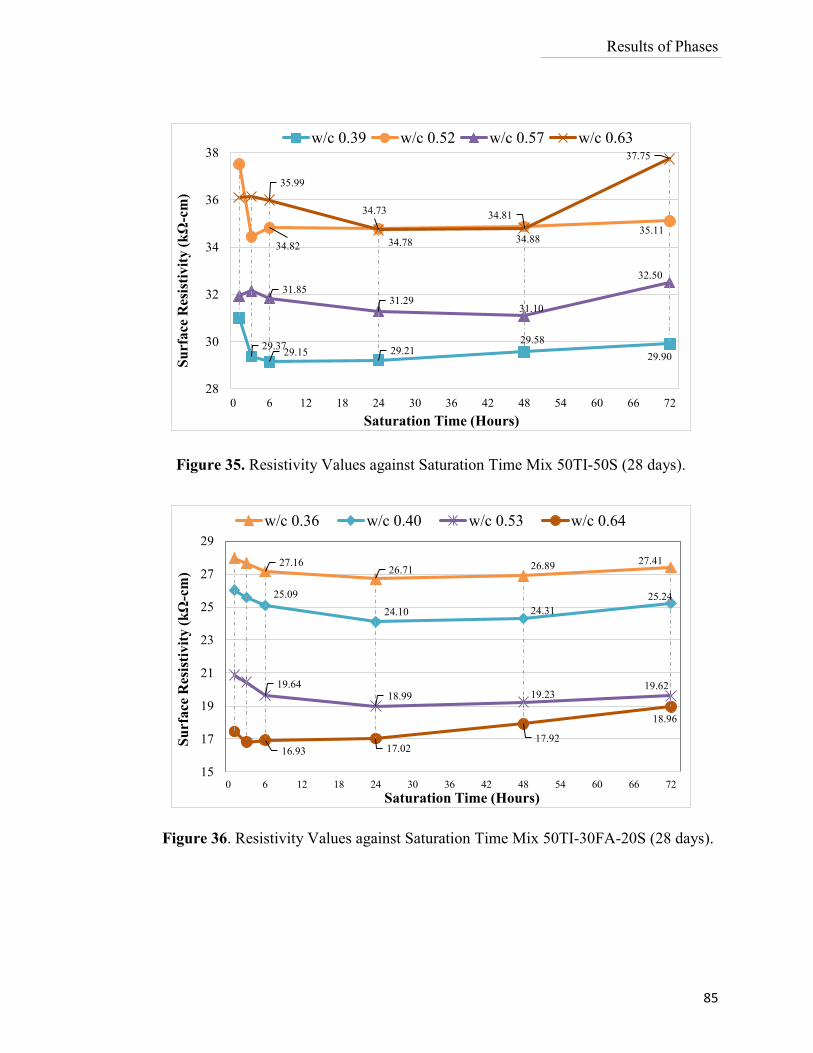
Results of Phases
85
Figure 36. Resistivity Values against Saturation Time Mix 50TI-30FA-20S (28 days).
27.1626.71 26.89
27.41
25.09
24.10 24.31
25.24
19.6418.99 19.23
19.62
16.93 17.0217.92
18.96
15
17
19
21
23
25
27
29
0 6 12 18 24 30 36 42 48 54 60 66 72
Su
rfa
ce
Res
isti
vit
y (
kΩ
-cm
)
Saturation Time (Hours)
w/c 0.36 w/c 0.40 w/c 0.53 w/c 0.64
Figure 35. Resistivity Values against Saturation Time Mix 50TI-50S (28 days).
29.3729.15 29.21
29.58
29.90
34.82 34.78 34.8835.11
31.8531.29
31.10
32.50
35.99
34.73 34.81
37.75
28
30
32
34
36
38
0 6 12 18 24 30 36 42 48 54 60 66 72
Su
rface
Res
isti
vit
y (
kΩ
-cm
)
Saturation Time (Hours)
w/c 0.39 w/c 0.52 w/c 0.57 w/c 0.63
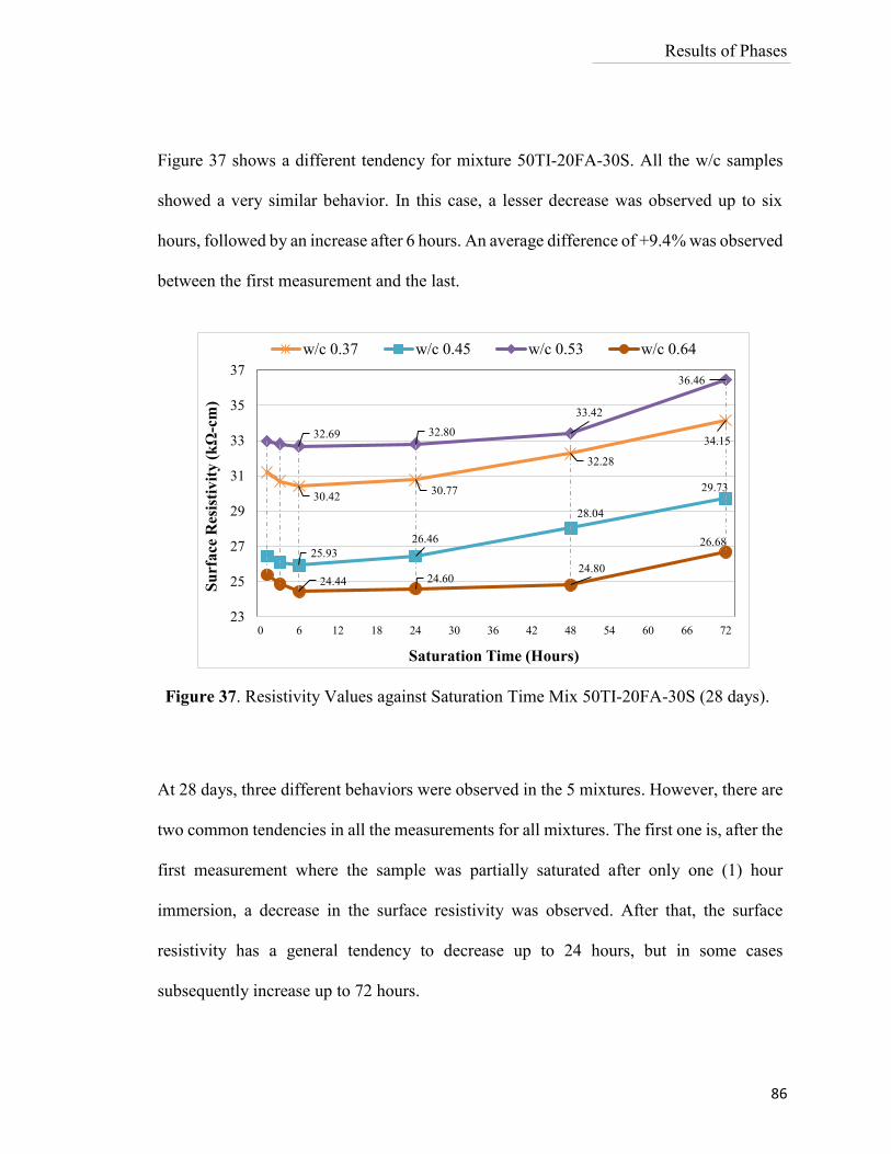
Results of Phases
86
Figure 37 shows a different tendency for mixture 50TI-20FA-30S. All the w/c samples
showed a very similar behavior. In this case, a lesser decrease was observed up to six
hours, followed by an increase after 6 hours. An average difference of +9.4% was observed
between the first measurement and the last.
At 28 days, three different behaviors were observed in the 5 mixtures. However, there are
two common tendencies in all the measurements for all mixtures. The first one is, after the
first measurement where the sample was partially saturated after only one (1) hour
immersion, a decrease in the surface resistivity was observed. After that, the surface
resistivity has a general tendency to decrease up to 24 hours, but in some cases
subsequently increase up to 72 hours.
Figure 37. Resistivity Values against Saturation Time Mix 50TI-20FA-30S (28 days).
30.4230.77
32.28
34.15
25.93
26.46
28.04
29.73
32.69 32.80
33.42
36.46
24.44 24.6024.80
26.68
23
25
27
29
31
33
35
37
0 6 12 18 24 30 36 42 48 54 60 66 72
Su
rface
Res
isti
vit
y (
kΩ
-cm
)
Saturation Time (Hours)
w/c 0.37 w/c 0.45 w/c 0.53 w/c 0.64
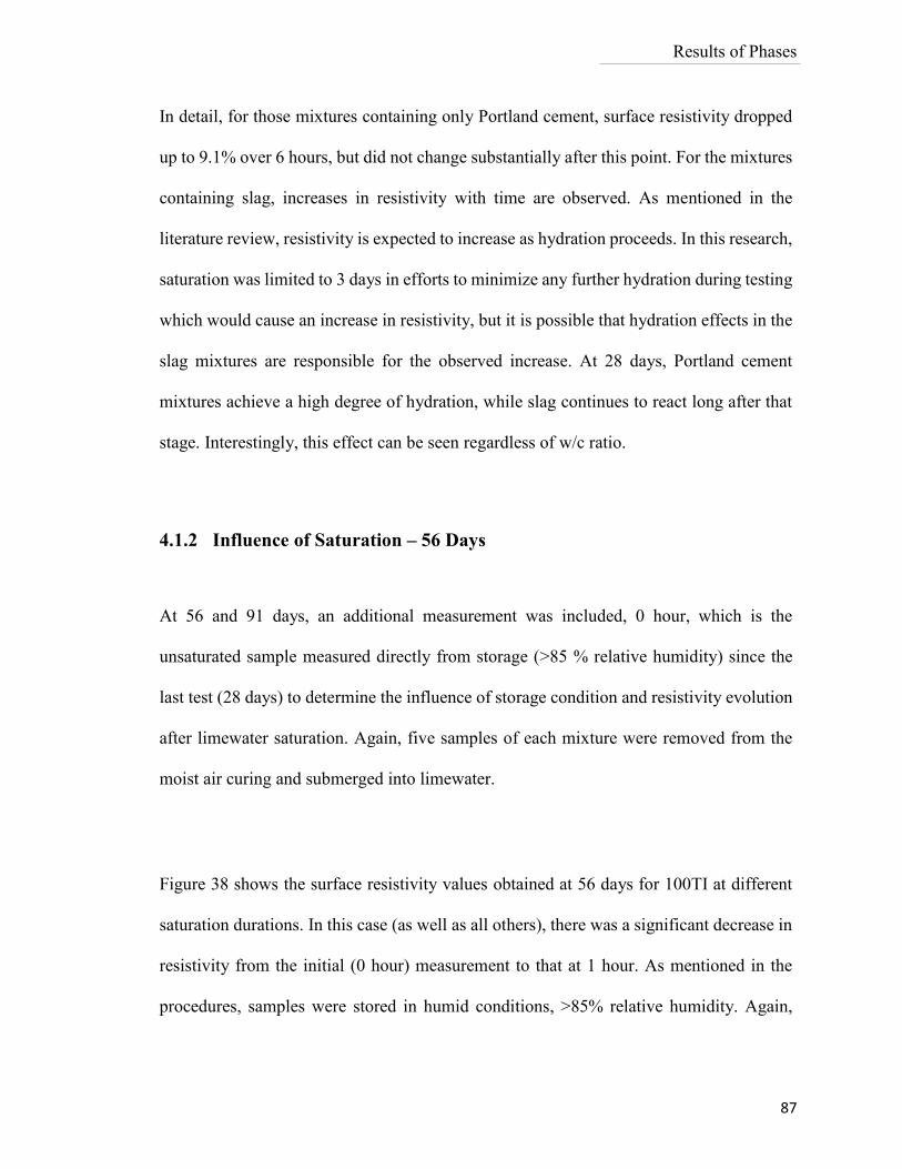
Results of Phases
87
In detail, for those mixtures containing only Portland cement, surface resistivity dropped
up to 9.1% over 6 hours, but did not change substantially after this point. For the mixtures
containing slag, increases in resistivity with time are observed. As mentioned in the
literature review, resistivity is expected to increase as hydration proceeds. In this research,
saturation was limited to 3 days in efforts to minimize any further hydration during testing
which would cause an increase in resistivity, but it is possible that hydration effects in the
slag mixtures are responsible for the observed increase. At 28 days, Portland cement
mixtures achieve a high degree of hydration, while slag continues to react long after that
stage. Interestingly, this effect can be seen regardless of w/c ratio.
4.1.2 Influence of Saturation – 56 Days
At 56 and 91 days, an additional measurement was included, 0 hour, which is the
unsaturated sample measured directly from storage (>85 % relative humidity) since the
last test (28 days) to determine the influence of storage condition and resistivity evolution
after limewater saturation. Again, five samples of each mixture were removed from the
moist air curing and submerged into limewater.
Figure 38 shows the surface resistivity values obtained at 56 days for 100TI at different
saturation durations. In this case (as well as all others), there was a significant decrease in
resistivity from the initial (0 hour) measurement to that at 1 hour. As mentioned in the
procedures, samples were stored in humid conditions, >85% relative humidity. Again,
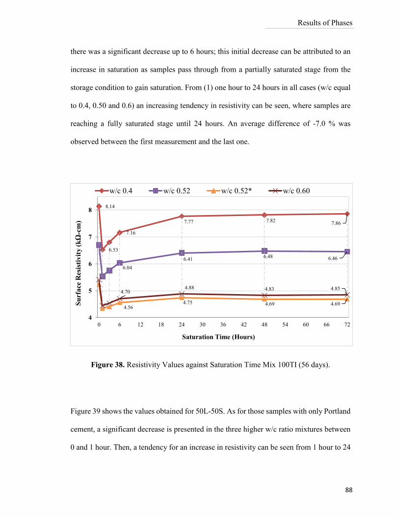
Results of Phases
88
there was a significant decrease up to 6 hours; this initial decrease can be attributed to an
increase in saturation as samples pass through from a partially saturated stage from the
storage condition to gain saturation. From (1) one hour to 24 hours in all cases (w/c equal
to 0.4, 0.50 and 0.6) an increasing tendency in resistivity can be seen, where samples are
reaching a fully saturated stage until 24 hours. An average difference of -7.0 % was
observed between the first measurement and the last one.
Figure 38. Resistivity Values against Saturation Time Mix 100TI (56 days).
Figure 39 shows the values obtained for 50L-50S. As for those samples with only Portland
cement, a significant decrease is presented in the three higher w/c ratio mixtures between
0 and 1 hour. Then, a tendency for an increase in resistivity can be seen from 1 hour to 24
8.14
6.53
7.16
7.77 7.827.86
6.04
6.416.48 6.46
4.564.75 4.69 4.69
4.704.88 4.83 4.85
4
5
6
7
8
0 6 12 18 24 30 36 42 48 54 60 66 72
Su
rface
Res
isti
vit
y (
kΩ
-cm
)
Saturation Time (Hours)
w/c 0.4 w/c 0.52 w/c 0.52* w/c 0.60
Results of Phases
89
hours for the same mixtures. After 24 hours, the resistivity tends to reach an asymptotic
value in all mixtures. An average difference of (–6.0 %) was observed between the first
measurement and the last one.
For those samples with 50TI-50S in Figure 40 it can be see that, the only common behavior
for the samples with different w/c (0.52, 0.54, 0.57, and 0.63) is after 24 hours where the
resistivity values reach a reasonably stable level. An average difference of (–7.0 %) was
observed between the first measurement and the last one.
Figure 39. Resistivity Values against Saturation Time Mix 50L-50S (56 days).
42.11 42.28 42.64
53.98
44.98
49.38
51.1650.61
46.04
48.9448.25
42.9843.89
43.67
37
40
43
46
49
52
55
0 6 12 18 24 30 36 42 48 54 60 66 72
Su
rface
Res
isti
vit
y (
kΩ
-cm
)
Saturation Time (Hours)
w/c 0.32 w/c 0.44 w/c 0.48 w/c 0.50
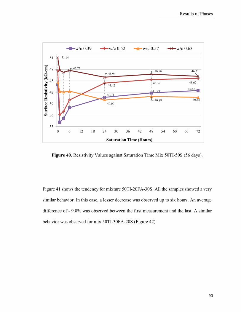
Results of Phases
90
Figure 41 shows the tendency for mixture 50TI-20FA-30S. All the samples showed a very
similar behavior. In this case, a lesser decrease was observed up to six hours. An average
difference of - 9.0% was observed between the first measurement and the last. A similar
behavior was observed for mix 50TI-30FA-20S (Figure 42).
Figure 40. Resistivity Values against Saturation Time Mix 50TI-50S (56 days).
40.7141.83
42.4644.42
45.32 45.62
40.0040.88 40.68
51.14
47.72
45.9446.76 46.21
33
36
39
42
45
48
51
0 6 12 18 24 30 36 42 48 54 60 66 72
Su
rface
Res
isti
vit
y (
kΩ
-cm
)
Saturation Time (Hours)
w/c 0.39 w/c 0.52 w/c 0.57 w/c 0.63
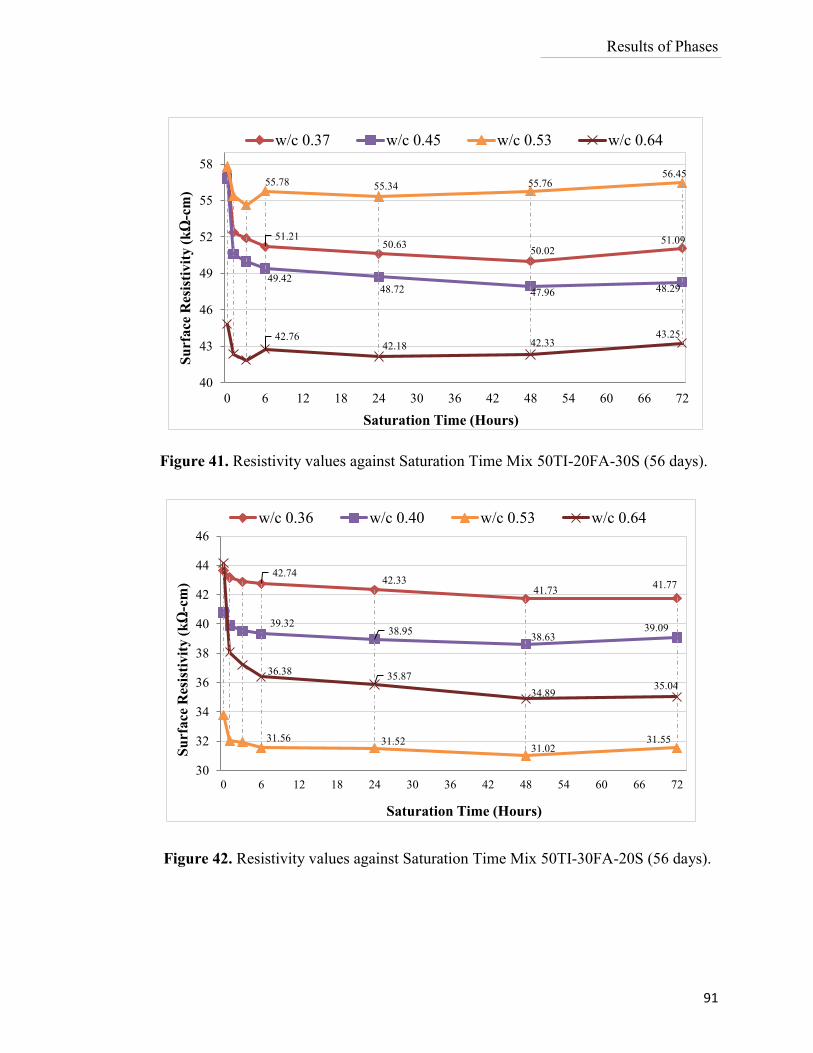
Results of Phases
91
Figure 42. Resistivity values against Saturation Time Mix 50TI-30FA-20S (56 days).
Figure 41. Resistivity values against Saturation Time Mix 50TI-20FA-30S (56 days).
51.2150.63
50.0251.09
49.4248.72 47.96 48.29
55.78 55.34 55.7656.45
42.7642.18 42.33
43.25
40
43
46
49
52
55
58
0 6 12 18 24 30 36 42 48 54 60 66 72
Su
rfa
ce R
esis
tiv
ity
(k
Ω-c
m)
Saturation Time (Hours)
w/c 0.37 w/c 0.45 w/c 0.53 w/c 0.64
42.7442.33
41.7341.77
39.3238.95
38.6339.09
31.56 31.5231.02
31.55
36.3835.87
34.8935.04
30
32
34
36
38
40
42
44
46
0 6 12 18 24 30 36 42 48 54 60 66 72
Su
rfa
ce R
esis
tivit
y (
kΩ
-cm
)
Saturation Time (Hours)
w/c 0.36 w/c 0.40 w/c 0.53 w/c 0.64
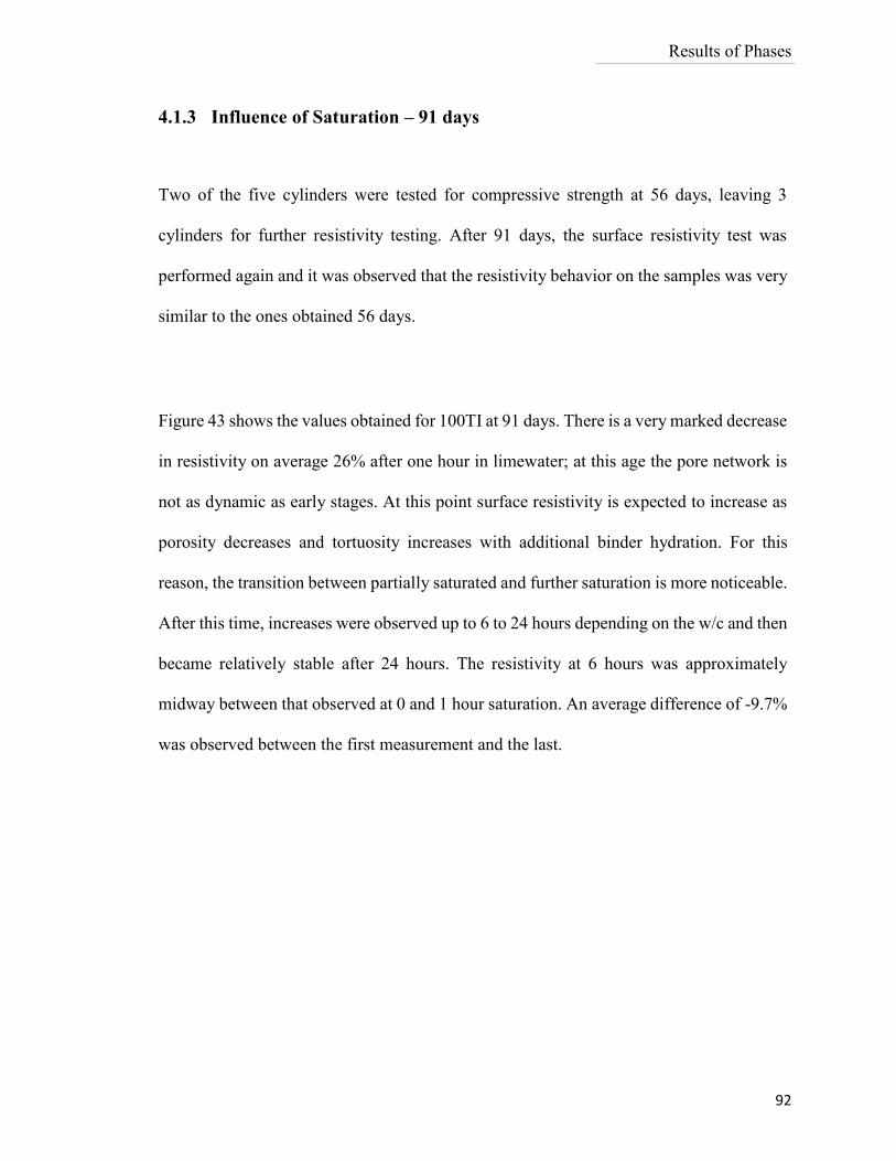
Results of Phases
92
4.1.3 Influence of Saturation – 91 days
Two of the five cylinders were tested for compressive strength at 56 days, leaving 3
cylinders for further resistivity testing. After 91 days, the surface resistivity test was
performed again and it was observed that the resistivity behavior on the samples was very
similar to the ones obtained 56 days.
Figure 43 shows the values obtained for 100TI at 91 days. There is a very marked decrease
in resistivity on average 26% after one hour in limewater; at this age the pore network is
not as dynamic as early stages. At this point surface resistivity is expected to increase as
porosity decreases and tortuosity increases with additional binder hydration. For this
reason, the transition between partially saturated and further saturation is more noticeable.
After this time, increases were observed up to 6 to 24 hours depending on the w/c and then
became relatively stable after 24 hours. The resistivity at 6 hours was approximately
midway between that observed at 0 and 1 hour saturation. An average difference of -9.7%
was observed between the first measurement and the last.
Results of Phases
93
Figures 44 and 45 shows the behavior at 91 days observed for 50TI–50S and 50TI-20FA-
30S, respectively. Again, most changes were observed up to 6 hours and then the values
were relatively stable after 24 hours. For the lowest two w/c, some small increases were
observed between 48 and 72 hours. The magnitude of the drop between the initial
measurement and that of 1 hour was similar to that observed in the 100TI mixture (on
average -26.4%). An average difference of -6.1% was observed between the first
measurement and the last.
7.33
8.088.31 8.23
6.03
6.56 6.60 6.63
4.84
5.00
4.90 4.91
4.60
4.72
4.77 4.72
4
5
6
7
8
9
0 6 12 18 24 30 36 42 48 54 60 66 72
Su
rface
Res
isti
vit
y (
kΩ
-cm
)
Saturation Time (Hours)
w/c 0.40 w/c 0.52 w/c 0.52* w/c 0.60
Figure 43. Resistivity Values against Saturation Time Mix 100TI (91 days).
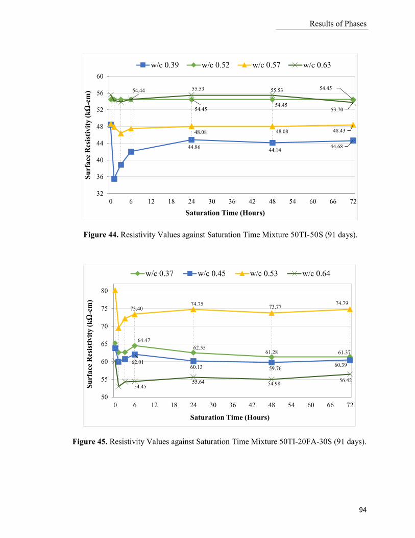
Results of Phases
94
44.8644.14
44.68
54.4554.45
54.45
48.08 48.08 48.43
54.44 55.53 55.53
53.70
32
36
40
44
48
52
56
60
0 6 12 18 24 30 36 42 48 54 60 66 72
Su
rfa
ce R
esis
tiv
ity
(k
Ω-c
m)
Saturation Time (Hours)
w/c 0.39 w/c 0.52 w/c 0.57 w/c 0.63
Figure 44. Resistivity Values against Saturation Time Mixture 50TI-50S (91 days).
64.47
62.5561.28 61.37
62.0160.13 59.76
60.39
73.4074.75
73.7774.79
54.4555.64 54.98
56.42
50
55
60
65
70
75
80
0 6 12 18 24 30 36 42 48 54 60 66 72
Su
rfa
ce R
esis
tivit
y (
kΩ
-cm
)
Saturation Time (Hours)
w/c 0.37 w/c 0.45 w/c 0.53 w/c 0.64
Figure 45. Resistivity Values against Saturation Time Mixture 50TI-20FA-30S (91 days).
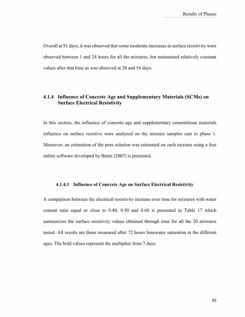
Results of Phases
95
Overall at 91 days, it was observed that some moderate increases in surface resistivity were
observed between 1 and 24 hours for all the mixtures, but maintained relatively constant
values after that time as was observed at 28 and 56 days.
4.1.4 Influence of Concrete Age and Supplementary Materials (SCMs) on
Surface Electrical Resistivity
In this section, the influence of concrete age and supplementary cementitious materials
influence on surface resistive were analyzed on the mixture samples cast in phase 1.
Moreover, an estimation of the pore solution was estimated on each mixture using a free
online software developed by Bentz (2007) is presented.
4.1.4.1 Influence of Concrete Age on Surface Electrical Resistivity
A comparison between the electrical resistivity increase over time for mixtures with water
cement ratio equal or close to 0.40, 0.50 and 0.60 is presented in Table 17 which
summarizes the surface resistivity values obtained through time for all the 20 mixtures
tested. All results are those measured after 72 hours limewater saturation at the different
ages. The bold values represent the multiplier from 7 days.
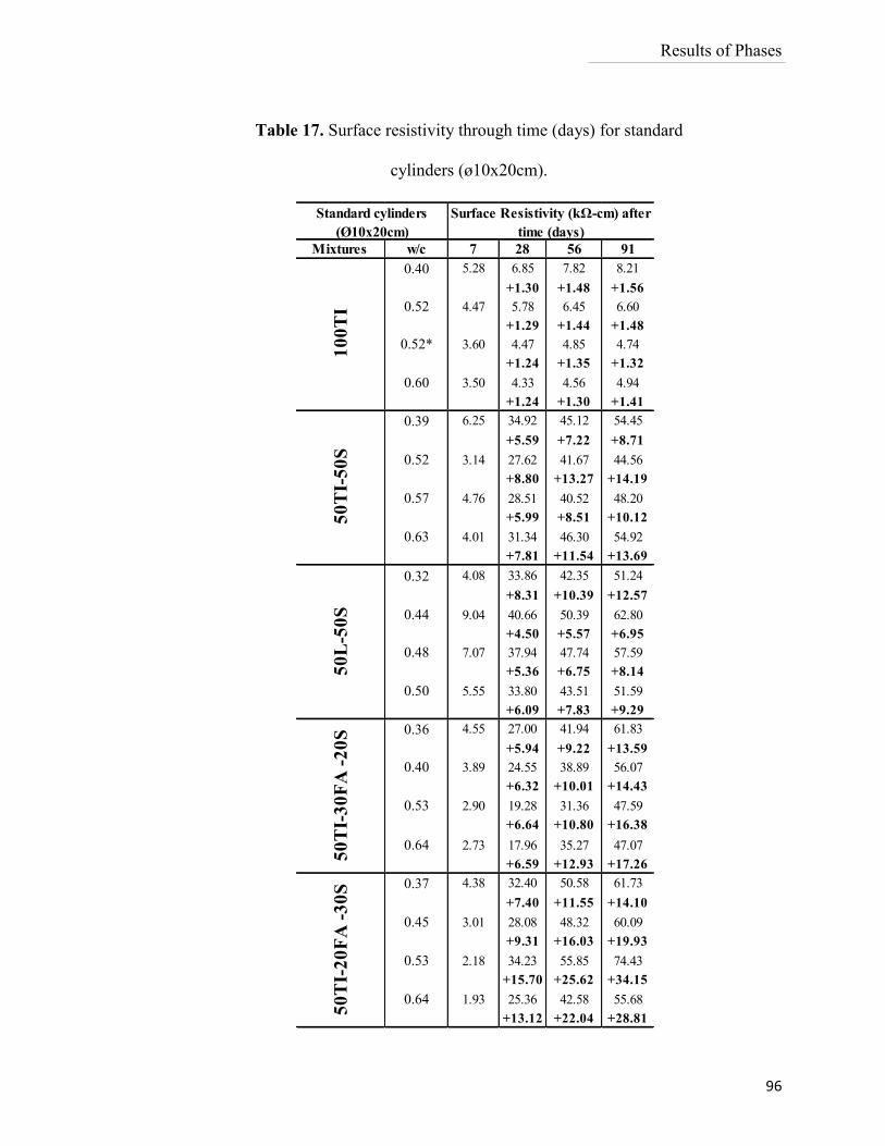
Results of Phases
96
Table 17. Surface resistivity through time (days) for standard
cylinders (ø10x20cm).
Mixtures w/c 91
0.40 5.28 6.85 7.82 8.21
+1.30 +1.48 +1.56
0.52 4.47 5.78 6.45 6.60
+1.29 +1.44 +1.48
0.52* 3.60 4.47 4.85 4.74
+1.24 +1.35 +1.32
0.60 3.50 4.33 4.56 4.94
+1.24 +1.30 +1.41
0.39 6.25 34.92 45.12 54.45
+5.59 +7.22 +8.71
0.52 3.14 27.62 41.67 44.56
+8.80 +13.27 +14.19
0.57 4.76 28.51 40.52 48.20
+5.99 +8.51 +10.12
0.63 4.01 31.34 46.30 54.92
+7.81 +11.54 +13.69
0.32 4.08 33.86 42.35 51.24
+8.31 +10.39 +12.57
0.44 9.04 40.66 50.39 62.80
+4.50 +5.57 +6.95
0.48 7.07 37.94 47.74 57.59
+5.36 +6.75 +8.14
0.50 5.55 33.80 43.51 51.59
+6.09 +7.83 +9.29
0.36 4.55 27.00 41.94 61.83
+5.94 +9.22 +13.59
0.40 3.89 24.55 38.89 56.07
+6.32 +10.01 +14.43
0.53 2.90 19.28 31.36 47.59
+6.64 +10.80 +16.38
0.64 2.73 17.96 35.27 47.07
+6.59 +12.93 +17.26
0.37 4.38 32.40 50.58 61.73
+7.40 +11.55 +14.10
0.45 3.01 28.08 48.32 60.09
+9.31 +16.03 +19.93
0.53 2.18 34.23 55.85 74.43
+15.70 +25.62 +34.15
0.64 1.93 25.36 42.58 55.68
+13.12 +22.04 +28.81
50
TI-
30
FA
-2
0S
50
TI-
20
FA
-3
0S
Surface Resistivity (kΩ-cm) after
time (days)
7 28 56
Standard cylinders
(Ø10x20cm)
10
0T
I5
0T
I-5
0S
50
L-5
0S
Results of Phases
97
For those samples with only Portland cement (100TI), the change is not as significant over
time as can be observed for those with fly ash and slag. An increment of 1.56 times higher
for the mixture 100TI w/c 0.40 was obtained between 7 to 91 days; for the mixture 50TI-
30FA-20S w/c 0.40 increment of 14.43 times higher was obtained.
Figure 46 shows the average values obtained for all mixtures with a water cement ratio
(w/c) close to 0.50. The electrical resistivity values obtained shows an accelerated
resistivity increase especially for those containing fly ash and slag. Mixture 100TI (100%
Portland cement) increases on average 1.48 times between the first measurement at 7 days
and the last at 91 days. But for those mixtures with fly ash and slag, the increase is more
significant; mixture 50TI- 50S during the same time the value increased on average 14.19
times higher, 50L-50S 9.29 times higher, 50TI30FA20S 16.38 and for those with
50TI20FA30S the value increased 34.15 times higher.
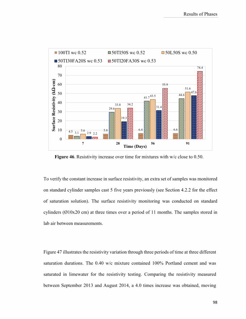
Results of Phases
98
To verify the constant increase in surface resistivity, an extra set of samples was monitored
on standard cylinder samples cast 5 five years previously (see Section 4.2.2 for the effect
of saturation solution). The surface resistivity monitoring was conducted on standard
cylinders (Ø10x20 cm) at three times over a period of 11 months. The samples stored in
lab air between measurements.
Figure 47 illustrates the resistivity variation through three periods of time at three different
saturation durations. The 0.40 w/c mixture contained 100% Portland cement and was
saturated in limewater for the resistivity testing. Comparing the resistivity measured
between September 2013 and August 2014, a 4.0 times increase was obtained, moving
4.5 5.8 6.4 6.63.1
29.6
41.744.6
5.6
33.8
43.5
51.6
2.9
19.3
31.4
47.6
2.2
34.2
55.9
74.4
0
10
20
30
40
50
60
70
80
7 28 56 91
Su
rface
Res
isti
vit
y (
kΩ
-cm
)
Time (Days)
100TI wc 0.52 50TI50S wc 0.52 50L50S wc 0.50
50TI30FA20S wc 0.53 50TI20FA30S wc 0.53
Figure 46. Resistivity increase over time for mixtures with w/c close to 0.50.
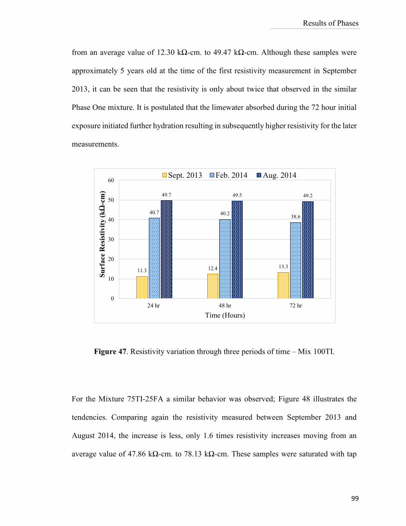
Results of Phases
99
from an average value of 12.30 kΩ-cm. to 49.47 kΩ-cm. Although these samples were
approximately 5 years old at the time of the first resistivity measurement in September
2013, it can be seen that the resistivity is only about twice that observed in the similar
Phase One mixture. It is postulated that the limewater absorbed during the 72 hour initial
exposure initiated further hydration resulting in subsequently higher resistivity for the later
measurements.
Figure 47. Resistivity variation through three periods of time – Mix 100TI.
For the Mixture 75TI-25FA a similar behavior was observed; Figure 48 illustrates the
tendencies. Comparing again the resistivity measured between September 2013 and
August 2014, the increase is less, only 1.6 times resistivity increases moving from an
average value of 47.86 kΩ-cm. to 78.13 kΩ-cm. These samples were saturated with tap
11.3 12.4 13.3
40.7 40.238.6
49.7 49.5 49.2
0
10
20
30
40
50
60
24 hr 48 hr 72 hr
Su
rface
Res
isti
vit
y (
kΩ
-cm
)
Time (Hours)
Sept. 2013 Feb. 2014 Aug. 2014
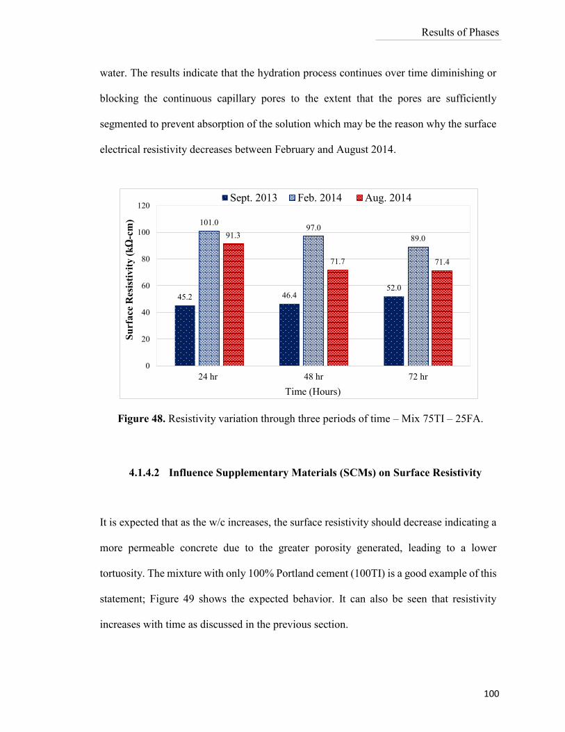
Results of Phases
100
water. The results indicate that the hydration process continues over time diminishing or
blocking the continuous capillary pores to the extent that the pores are sufficiently
segmented to prevent absorption of the solution which may be the reason why the surface
electrical resistivity decreases between February and August 2014.
4.1.4.2 Influence Supplementary Materials (SCMs) on Surface Resistivity
It is expected that as the w/c increases, the surface resistivity should decrease indicating a
more permeable concrete due to the greater porosity generated, leading to a lower
tortuosity. The mixture with only 100% Portland cement (100TI) is a good example of this
statement; Figure 49 shows the expected behavior. It can also be seen that resistivity
increases with time as discussed in the previous section.
45.2 46.452.0
101.097.0
89.091.3
71.7 71.4
0
20
40
60
80
100
120
24 hr 48 hr 72 hr
Su
rface
Res
isti
vit
y (
kΩ
-cm
)
Time (Hours)
Sept. 2013 Feb. 2014 Aug. 2014
Figure 48. Resistivity variation through three periods of time – Mix 75TI – 25FA.
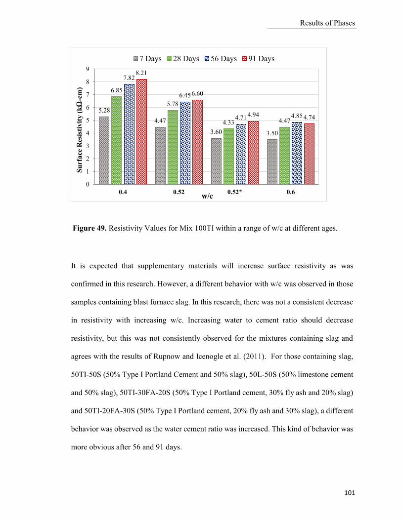
Results of Phases
101
It is expected that supplementary materials will increase surface resistivity as was
confirmed in this research. However, a different behavior with w/c was observed in those
samples containing blast furnace slag. In this research, there was not a consistent decrease
in resistivity with increasing w/c. Increasing water to cement ratio should decrease
resistivity, but this was not consistently observed for the mixtures containing slag and
agrees with the results of Rupnow and Icenogle et al. (2011). For those containing slag,
50TI-50S (50% Type I Portland Cement and 50% slag), 50L-50S (50% limestone cement
and 50% slag), 50TI-30FA-20S (50% Type I Portland cement, 30% fly ash and 20% slag)
and 50TI-20FA-30S (50% Type I Portland cement, 20% fly ash and 30% slag), a different
behavior was observed as the water cement ratio was increased. This kind of behavior was
more obvious after 56 and 91 days.
5.28
4.47
3.60 3.50
6.85
5.78
4.33 4.47
7.82
6.45
4.71 4.85
8.21
6.60
4.94 4.74
0
1
2
3
4
5
6
7
8
9
0.4 0.52 0.52* 0.6
Su
rfa
ce R
esis
tiv
ity
(k
Ω-c
m)
w/c
7 Days 28 Days 56 Days 91 Days
Figure 49. Resistivity Values for Mix 100TI within a range of w/c at different ages.
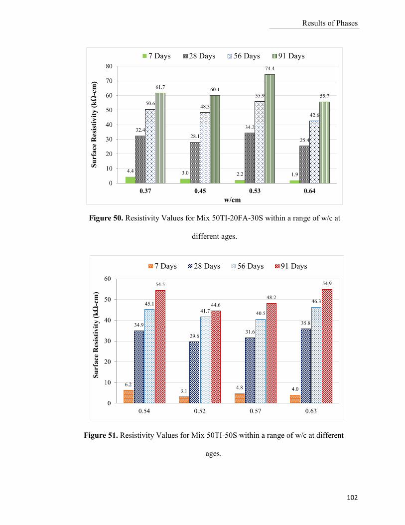
Results of Phases
102
Figure 51. Resistivity Values for Mix 50TI-50S within a range of w/c at different
ages.
4.4 3.0 2.2 1.9
32.4
28.1
34.2
25.4
50.648.3
55.9
42.6
61.7 60.1
74.4
55.7
0
10
20
30
40
50
60
70
80
0.37 0.45 0.53 0.64
Su
rfa
ce R
esis
tiv
ity
(k
Ω-c
m)
w/cm
7 Days 28 Days 56 Days 91 Days
6.2
3.14.8 4.0
34.9
29.631.6
35.8
45.1
41.7 40.5
46.3
54.5
44.6
48.2
54.9
0
10
20
30
40
50
60
0.54 0.52 0.57 0.63
Su
rfa
ce R
esis
tivit
y (
kΩ
-cm
)
7 Days 28 Days 56 Days 91 Days
Figure 50. Resistivity Values for Mix 50TI-20FA-30S within a range of w/c at
different ages.
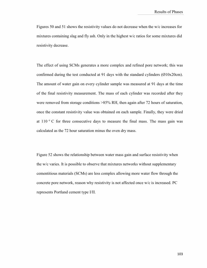
Results of Phases
103
Figures 50 and 51 shows the resistivity values do not decrease when the w/c increases for
mixtures containing slag and fly ash. Only in the highest w/c ratios for some mixtures did
resistivity decrease.
The effect of using SCMs generates a more complex and refined pore network; this was
confirmed during the test conducted at 91 days with the standard cylinders (Ø10x20cm).
The amount of water gain on every cylinder sample was measured at 91 days at the time
of the final resistivity measurement. The mass of each cylinder was recorded after they
were removed from storage conditions >85% RH, then again after 72 hours of saturation,
once the constant resistivity value was obtained on each sample. Finally, they were dried
at 110 o C for three consecutive days to measure the final mass. The mass gain was
calculated as the 72 hour saturation minus the oven dry mass.
Figure 52 shows the relationship between water mass gain and surface resistivity when
the w/c varies. It is possible to observe that mixtures networks without supplementary
cementitious materials (SCMs) are less complex allowing more water flow through the
concrete pore network, reason why resistivity is not affected once w/c is increased. PC
represents Portland cement type I/II.
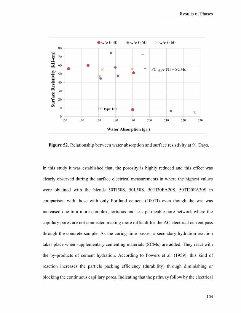
Results of Phases
104
In this study it was established that, the porosity is highly reduced and this effect was
clearly observed during the surface electrical measurements in where the highest values
were obtained with the blends 50TI50S, 50L50S, 50TI30FA20S, 50TI20FA30S in
comparison with those with only Portland cement (100TI) even though the w/c was
increased due to a more complex, tortuous and less permeable pore network where the
capillary pores are not connected making more difficult for the AC electrical current pass
through the concrete sample. As the curing time passes, a secondary hydration reaction
takes place when supplementary cementing materials (SCMs) are added. They react with
the by-products of cement hydration. According to Powers et al. (1959), this kind of
reaction increases the particle packing efficiency (durability) through diminishing or
blocking the continuous capillary pores. Indicating that the pathway follow by the electrical
Figure 52. Relationship between water absorption and surface resistivity at 91 Days.
0
10
20
30
40
50
60
70
80
150 160 170 180 190 200 210 220 230
Su
rface
Res
isti
vit
y (
kΩ
-cm
)
Water Absorption (gr.)
w/c 0.40 w/c 0.50 w/c 0.60
PC type I/II
PC type I/II + SCMs
Results of Phases
105
current is more tortuous due to the porous network reduction, where the possibility of
chloride or sulphate attack, corrosion, or concrete degradation is minimized achieving
negligible penetrability risk.
Besides the changes in porosity, the use of supplementary cementitious materials (SCMs)
have an important influence on surface resistivity and compressive strength. A higher
resistivity is related to higher compressive strength. According to the samples studied by
Shahroodi (2010), lowering the w/c increases the compressive strength by 16% whereas
the surface resistivity was increased by up to 60% at the same age.
4.1.4.2.1 Pore solution conductivity
The results indicate that surface resistivity values are clearly affected by the use of fly ash
and slag. According to Nokken et al. (2006), at early ages the connectivity of the pore
structure and pore size distribution is dynamically changing and the ionic concentration in
the pore solution increases with age, generating higher electrical conductivity (lower
resistivity) during the first 28 days.
As was mentioned before, pore solution chemistry in cementitious materials varies with
mixture design and time. The National Institute of Standards and Technology (NIST)
developed a technique to determine the conductivity of the pore solution using the
concentration of different ionic species (Snyder et al., 2003).
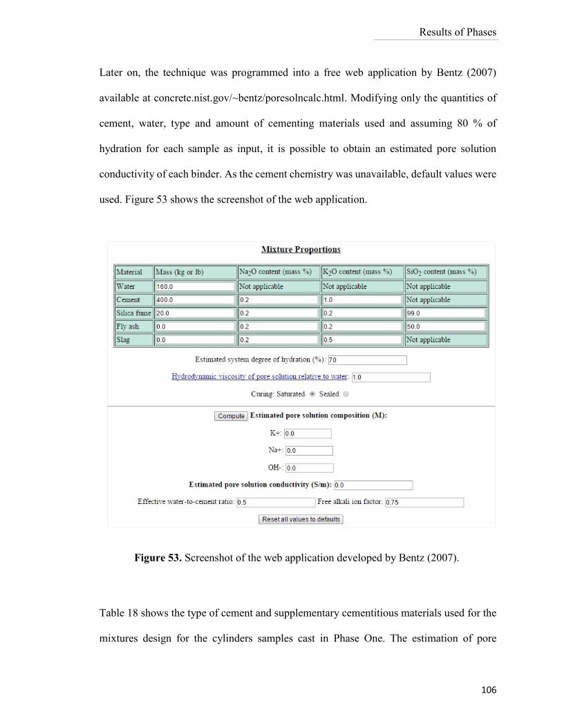
Results of Phases
106
Later on, the technique was programmed into a free web application by Bentz (2007)
available at concrete.nist.gov/~bentz/poresolncalc.html. Modifying only the quantities of
cement, water, type and amount of cementing materials used and assuming 80 % of
hydration for each sample as input, it is possible to obtain an estimated pore solution
conductivity of each binder. As the cement chemistry was unavailable, default values were
used. Figure 53 shows the screenshot of the web application.
Table 18 shows the type of cement and supplementary cementitious materials used for the
mixtures design for the cylinders samples cast in Phase One. The estimation of pore
Figure 53. Screenshot of the web application developed by Bentz (2007).
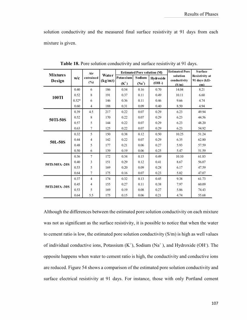
Results of Phases
107
solution conductivity and the measured final surface resistivity at 91 days from each
mixture is given.
Although the differences between the estimated pore solution conductivity on each mixture
was not as significant as the surface resistivity, it is possible to notice that when the water
to cement ratio is low, the estimated pore solution conductivity (S/m) is high as well values
of individual conductive ions, Potassium (K+), Sodium (Na+ ), and Hydroxide (OH-). The
opposite happens when water to cement ratio is high, the conductivity and conductive ions
are reduced. Figure 54 shows a comparison of the estimated pore solution conductivity and
surface electrical resistivity at 91 days. For instance, those with only Portland cement
0.40 6 186 0.54 0.16 0.70 14.04 8.21
0.52 8 191 0.37 0.11 0.49 10.11 6.60
0.52* 6 146 0.36 0.11 0.46 9.66 4.74
0.60 4 188 0.31 0.09 0.40 8.50 4.94
0.39 4.5 217 0.22 0.07 0.29 6.23 49.94
0.52 8 170 0.22 0.07 0.29 6.23 44.56
0.57 5 144 0.22 0.07 0.29 6.23 48.20
0.63 7 125 0.22 0.07 0.29 6.23 54.92
0.32 5 150 0.38 0.12 0.50 10.25 51.24
0.44 4 142 0.22 0.07 0.29 6.35 62.80
0.48 5 177 0.21 0.06 0.27 5.93 57.59
0.50 6 139 0.19 0.06 0.25 5.47 51.59
0.36 7 172 0.34 0.15 0.49 10.10 61.83
0.40 3 151 0.29 0.12 0.41 8.67 56.07
0.53 5 169 0.20 0.09 0.28 6.17 47.59
0.64 7 175 0.16 0.07 0.23 5.02 47.07
0.37 4 174 0.32 0.13 0.45 9.38 61.73
0.45 4 155 0.27 0.11 0.38 7.97 60.09
0.53 5 169 0.19 0.08 0.27 5.86 74.43
0.64 5.5 175 0.15 0.06 0.21 4.74 55.68
Estimated Pore solution (M) Estimated Pore
solution
conductivity
(S /m)
50TI-20FA -30S
Hydroxide
(OH -)
100TI
50TI-50S
50L-50S
50TI-30FA -20S
Mixtures
Designw/c
Air
entrained
(%)
Water
(kg/m3)
Surface
Resistivity at
91 days (kΩ-
cm)
Potassium
(K+
)
Sodium
(Na+)
Table 18. Pore solution conductivity and surface resistivity at 91 days.
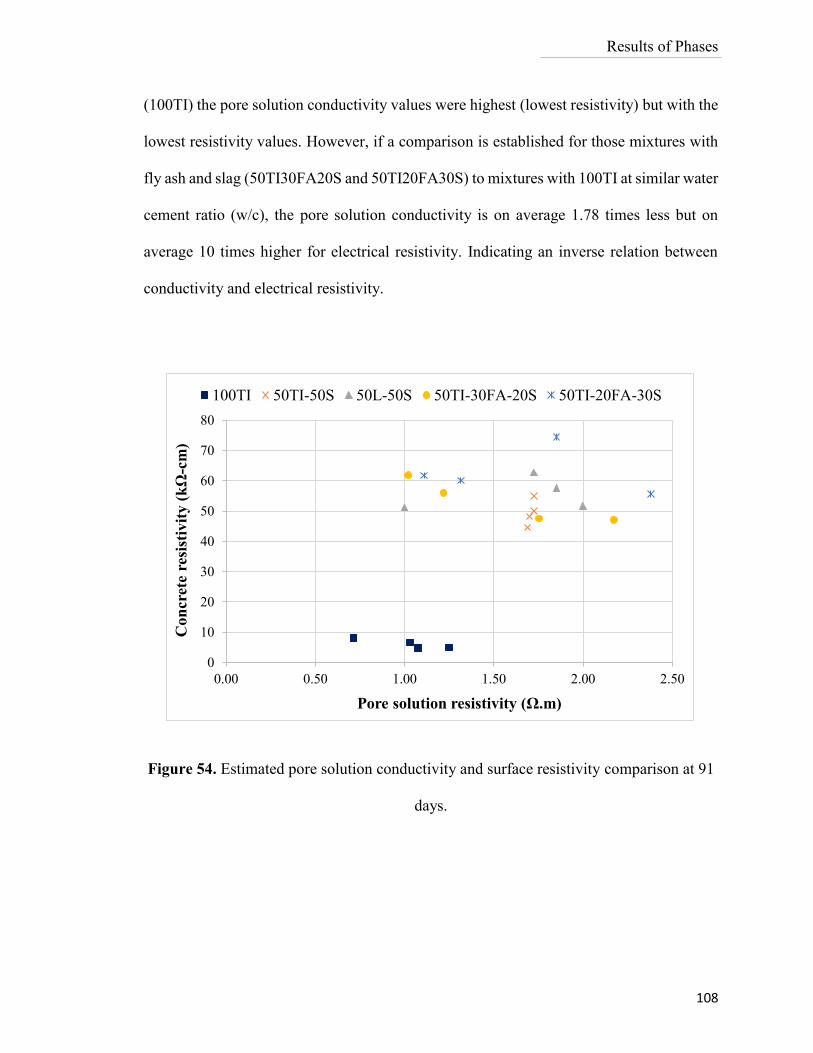
Results of Phases
108
(100TI) the pore solution conductivity values were highest (lowest resistivity) but with the
lowest resistivity values. However, if a comparison is established for those mixtures with
fly ash and slag (50TI30FA20S and 50TI20FA30S) to mixtures with 100TI at similar water
cement ratio (w/c), the pore solution conductivity is on average 1.78 times less but on
average 10 times higher for electrical resistivity. Indicating an inverse relation between
conductivity and electrical resistivity.
Figure 54. Estimated pore solution conductivity and surface resistivity comparison at 91
days.
0
10
20
30
40
50
60
70
80
0.00 0.50 1.00 1.50 2.00 2.50
Con
cret
e re
sist
ivit
y (
kΩ
-cm
)
Pore solution resistivity (Ω.m)
100TI 50TI-50S 50L-50S 50TI-30FA-20S 50TI-20FA-30S
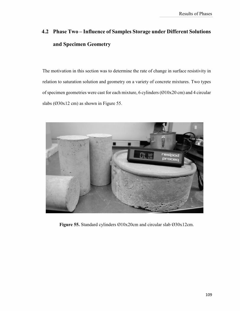
Results of Phases
109
4.2 Phase Two – Influence of Samples Storage under Different Solutions
and Specimen Geometry
The motivation in this section was to determine the rate of change in surface resistivity in
relation to saturation solution and geometry on a variety of concrete mixtures. Two types
of specimen geometries were cast for each mixture, 6 cylinders (Ø10x20 cm) and 4 circular
slabs (Ø30x12 cm) as shown in Figure 55.
Figure 55. Standard cylinders Ø10x20cm and circular slab Ø30x12cm.
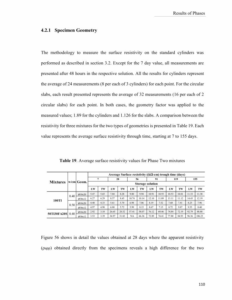
Results of Phases
110
4.2.1 Specimen Geometry
The methodology to measure the surface resistivity on the standard cylinders was
performed as described in section 3.2. Except for the 7 day value, all measurements are
presented after 48 hours in the respective solution. All the results for cylinders represent
the average of 24 measurements (8 per each of 3 cylinders) for each point. For the circular
slabs, each result presented represents the average of 32 measurements (16 per each of 2
circular slabs) for each point. In both cases, the geometry factor was applied to the
measured values; 1.89 for the cylinders and 1.126 for the slabs. A comparison between the
resistivity for three mixtures for the two types of geometries is presented in Table 19. Each
value represents the average surface resistivity through time, starting at 7 to 155 days.
Figure 56 shows in detail the values obtained at 28 days where the apparent resistivity
(ρapp) obtained directly from the specimens reveals a high difference for the two
LW TW LW TW LW TW LW TW LW TW LW TW
ø10x20 5.47 5.65 7.84 8.28 9.80 9.94 10.91 10.55 10.53 10.81 11.33 11.38
ø30x12 6.27 6.29 8.57 8.45 10.74 10.14 12.10 11.09 13.11 11.12 14.43 12.19
ø10x20 4.48 4.33 5.61 5.70 6.98 7.06 8.19 7.52 7.60 7.41 8.25 7.96
ø30x12 4.97 4.98 6.88 5.72 5.99 8.15 8.67 7.15 8.72 9.87 9.55 8.40
ø10x20 2.92 3.10 26.65 28.52 57.41 58.07 76.12 69.46 74.84 72.19 92.79 88.88
ø30x12 3.53 3.39 34.97 31.82 NA 66.36 72.89 74.41 77.80 84.93 96.36 106.23
0.40
0.50
0.40
100TI
50TI30FA20S
Mixtures w/cm Geom.
Average Surface resistivity ((kΩ-cm) trough time (days)
7 28 56 91 119 155
Storage solution
Table 19. Average surface resistivity values for Phase Two mixtures
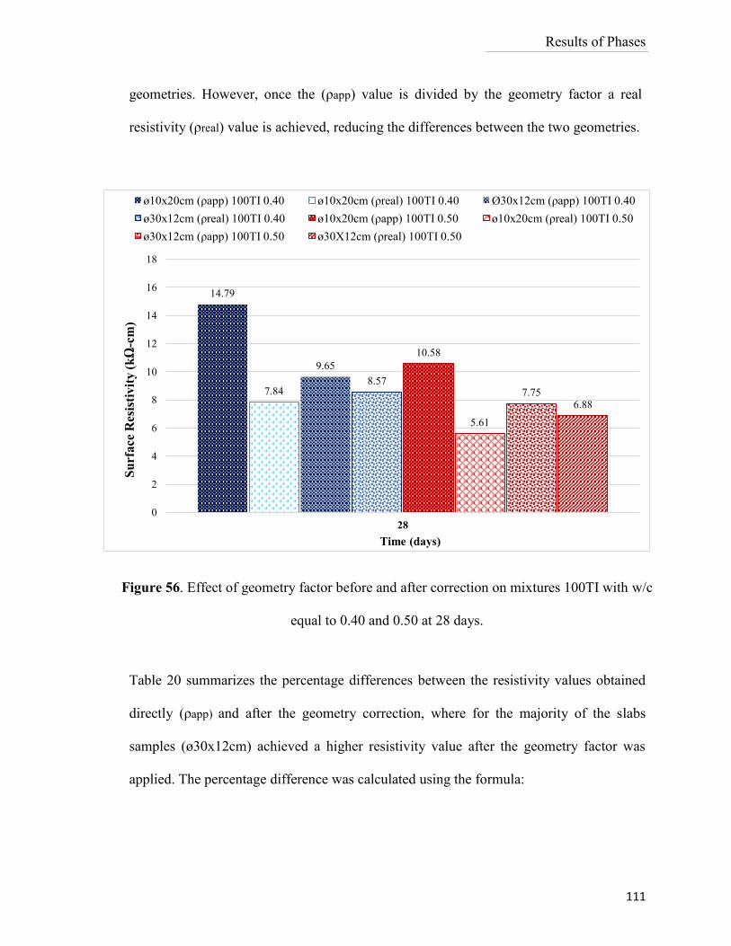
Results of Phases
111
geometries. However, once the (ρapp) value is divided by the geometry factor a real
resistivity (ρreal) value is achieved, reducing the differences between the two geometries.
Table 20 summarizes the percentage differences between the resistivity values obtained
directly (ρapp) and after the geometry correction, where for the majority of the slabs
samples (ø30x12cm) achieved a higher resistivity value after the geometry factor was
applied. The percentage difference was calculated using the formula:
14.79
7.84
9.65
8.57
10.58
5.61
7.756.88
0
2
4
6
8
10
12
14
16
18
28
Su
rface
Res
isti
vit
y (
kΩ
-cm
)
Time (days)
ø10x20cm (ρapp) 100TI 0.40 ø10x20cm (ρreal) 100TI 0.40 Ø30x12cm (ρapp) 100TI 0.40
ø30x12cm (ρreal) 100TI 0.40 ø10x20cm (ρapp) 100TI 0.50 ø10x20cm (ρreal) 100TI 0.50
ø30x12cm (ρapp) 100TI 0.50 ø30X12cm (ρreal) 100TI 0.50
Figure 56. Effect of geometry factor before and after correction on mixtures 100TI with w/c
equal to 0.40 and 0.50 at 28 days.
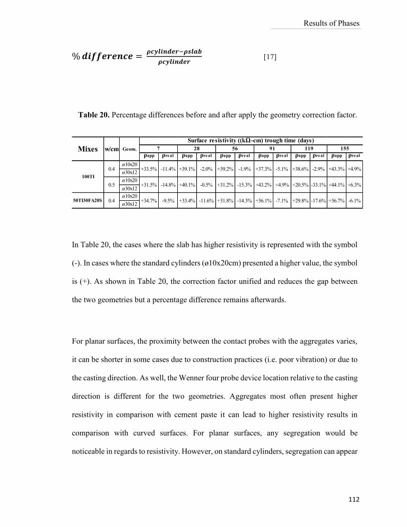
Results of Phases
112
% 𝒅𝒊𝒇𝒇𝒆𝒓𝒆𝒏𝒄𝒆 = 𝝆𝒄𝒚𝒍𝒊𝒏𝒅𝒆𝒓−𝝆𝒔𝒍𝒂𝒃
𝝆𝒄𝒚𝒍𝒊𝒏𝒅𝒆𝒓 [17]
In Table 20, the cases where the slab has higher resistivity is represented with the symbol
(-). In cases where the standard cylinders (ø10x20cm) presented a higher value, the symbol
is (+). As shown in Table 20, the correction factor unified and reduces the gap between
the two geometries but a percentage difference remains afterwards.
For planar surfaces, the proximity between the contact probes with the aggregates varies,
it can be shorter in some cases due to construction practices (i.e. poor vibration) or due to
the casting direction. As well, the Wenner four probe device location relative to the casting
direction is different for the two geometries. Aggregates most often present higher
resistivity in comparison with cement paste it can lead to higher resistivity results in
comparison with curved surfaces. For planar surfaces, any segregation would be
noticeable in regards to resistivity. However, on standard cylinders, segregation can appear
ρapp ρreal ρapp ρreal ρapp ρreal ρapp ρreal ρapp ρreal ρapp ρreal
ø10x20
ø30x12
ø10x20
ø30x12
ø10x20
ø30x12
Surface resistivity ((kΩ-cm) trough time (days)
Geom.w/cmMixes 7 28 56
50TI30FA20S 0.4 +34.7% -9.5% +33.4% -11.6%
+4.9%
0.5 +31.5% -14.8% +40.1% -0.5% +31.2% -15.3% +43.2% +4.9%
-1.9% +37.3% -5.1% +38.6% -2.9% +43.3%
100TI
0.4
+36.7% -6.1%+31.8% -14.3% +36.1% -7.1% +29.8% -17.6%
+20.5% -33.1% +44.1% +6.3%
91 119 155
+33.5% -11.4% +39.1% -2.0% +39.2%
Table 20. Percentage differences before and after apply the geometry correction factor.
Results of Phases
113
at the bottom of the cylinder but the Wenner probe device is located along the depth of the
specimen.
4.2.1.1 City of Montreal (Ville de Montréal) Laboratory Samples
In addition to the samples cast for this research at Concordia University laboratory, another
sets of samples were tested from a sidewalk project conducted by the City of Montreal
(Ville de Montréal) and Sherbrooke University as was mentioned before in section 3.2.
All the samples were cast on October 2nd 2013 and afterwards stored in a fog room with a
constant 99% RH at 21 o C. Figure 57 shows the surface electrical resistivity obtained 336
days after casting. The samples were measured directly from the fog room and not further
saturated. Each value shown represents an average of a direct measurement from 22
cylinders (ø10x20cm) and 4 cylinders (ø15x30cm) mixture sample VdeMTL Temoin
(GU), 8 cylinders (ø10x20cm) and 4 cylinders (ø15x30cm) for mixture samples VdeMTL
25PV and 10PV, respectively. In the same figure, (ρ app) represents the resistivity
measured directly without the geometry correction factor and (ρ real) after the geometry
correction factor (k) was applied.
All resistivity values were calculated to include the correction factor as mentioned in
section 2.2.3 when 𝑑 𝑎⁄ ≤ 6 or 𝐿 𝑎⁄ ≥ 6. For ø10x20cm cylinders the correction value is
1.89 and for ø15x30cm, the correction value is 1.39. Again after the cell correction was
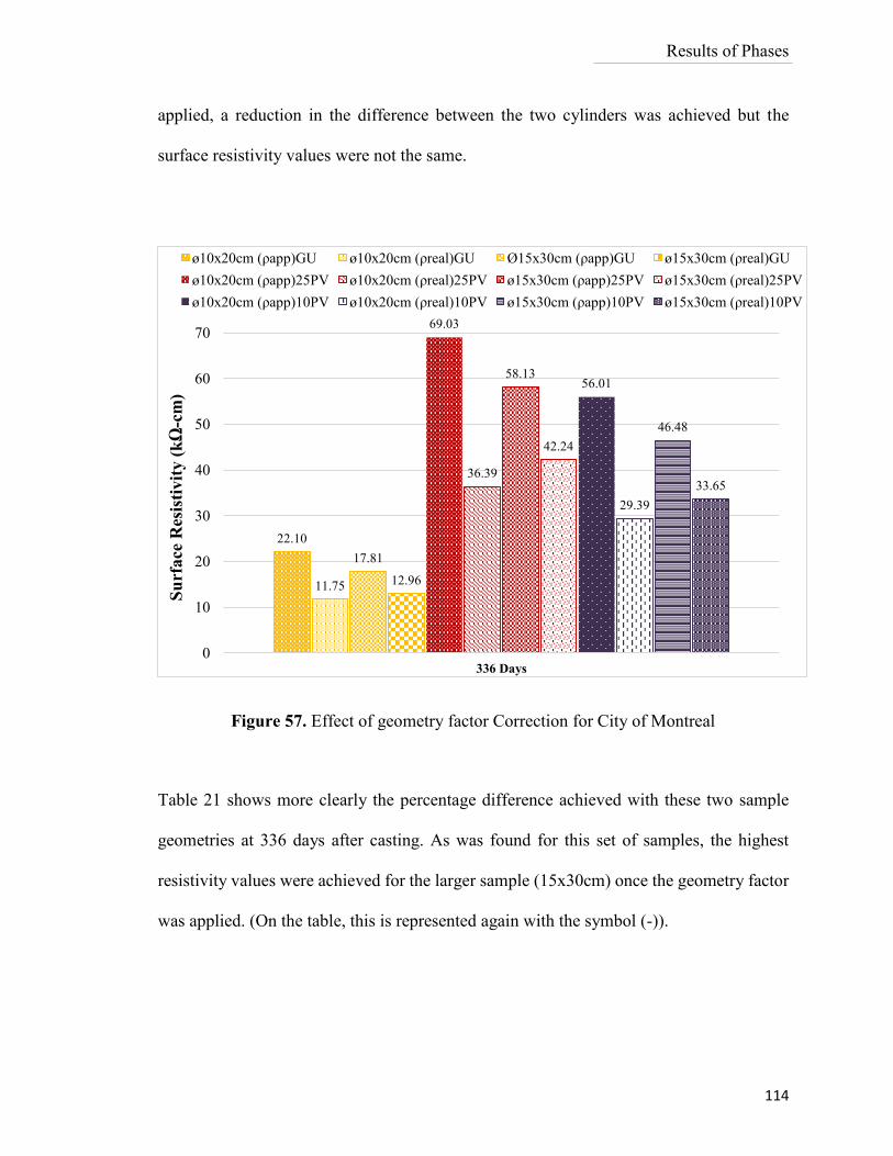
Results of Phases
114
applied, a reduction in the difference between the two cylinders was achieved but the
surface resistivity values were not the same.
Table 21 shows more clearly the percentage difference achieved with these two sample
geometries at 336 days after casting. As was found for this set of samples, the highest
resistivity values were achieved for the larger sample (15x30cm) once the geometry factor
was applied. (On the table, this is represented again with the symbol (-)).
22.10
11.75
17.81
12.96
69.03
36.39
58.13
42.24
56.01
29.39
46.48
33.65
0
10
20
30
40
50
60
70
336 Days
Su
rface
Res
isti
vit
y (
kΩ
-cm
)
ø10x20cm (ρapp)GU ø10x20cm (ρreal)GU Ø15x30cm (ρapp)GU ø15x30cm (ρreal)GU
ø10x20cm (ρapp)25PV ø10x20cm (ρreal)25PV ø15x30cm (ρapp)25PV ø15x30cm (ρreal)25PV
ø10x20cm (ρapp)10PV ø10x20cm (ρreal)10PV ø15x30cm (ρapp)10PV ø15x30cm (ρreal)10PV
Figure 57. Effect of geometry factor Correction for City of Montreal
samples.
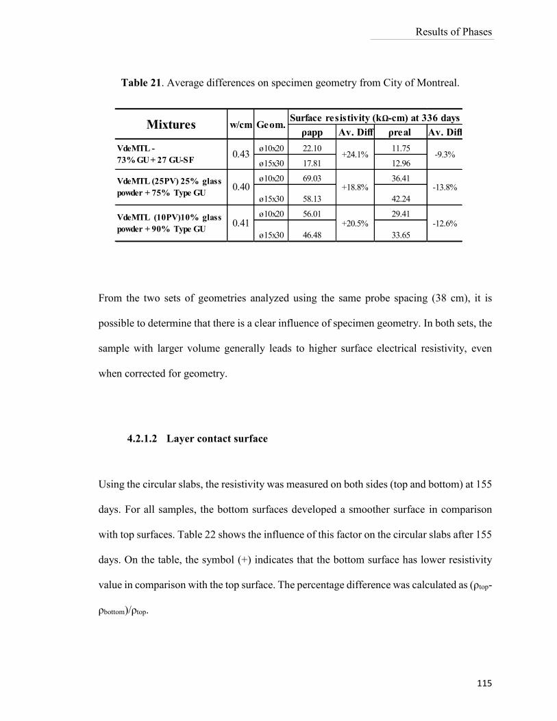
Results of Phases
115
From the two sets of geometries analyzed using the same probe spacing (38 cm), it is
possible to determine that there is a clear influence of specimen geometry. In both sets, the
sample with larger volume generally leads to higher surface electrical resistivity, even
when corrected for geometry.
4.2.1.2 Layer contact surface
Using the circular slabs, the resistivity was measured on both sides (top and bottom) at 155
days. For all samples, the bottom surfaces developed a smoother surface in comparison
with top surfaces. Table 22 shows the influence of this factor on the circular slabs after 155
days. On the table, the symbol (+) indicates that the bottom surface has lower resistivity
value in comparison with the top surface. The percentage difference was calculated as (ρtop-
ρbottom)/ρtop.
ρapp Av. Diff ρreal Av. Diff
ø10x20 22.10 11.75
ø15x30 17.81 12.96
ø10x20 69.03 36.41
ø15x30 58.13 42.24
ø10x20 56.01 29.41
ø15x30 46.48 33.65
Surface resistivity (kΩ-cm) at 336 daysMixtures w/cm Geom.
VdeMTL (10PV)10% glass
powder + 90% Type GU0.41
VdeMTL (25PV) 25% glass
powder + 75% Type GU
VdeMTL -
73% GU + 27 GU-SF0.43
0.40
+24.1%
+18.8%
+20.5%
-9.3%
-13.8%
-12.6%
Table 21. Average differences on specimen geometry from City of Montreal.
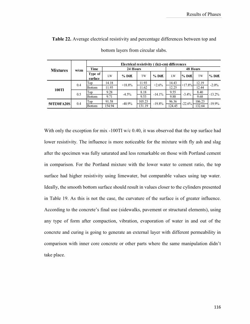
Results of Phases
116
With only the exception for mix -100TI w/c 0.40, it was observed that the top surface had
lower resistivity. The influence is more noticeable for the mixture with fly ash and slag
after the specimen was fully saturated and less remarkable on those with Portland cement
in comparison. For the Portland mixture with the lower water to cement ratio, the top
surface had higher resistivity using limewater, but comparable values using tap water.
Ideally, the smooth bottom surface should result in values closer to the cylinders presented
in Table 19. As this is not the case, the curvature of the surface is of greater influence.
According to the concrete’s final use (sidewalks, pavement or structural elements), using
any type of form after compaction, vibration, evaporation of water in and out of the
concrete and curing is going to generate an external layer with different permeability in
comparison with inner core concrete or other parts where the same manipulation didn’t
take place.
Time
Top 14.18 11.93 14.43 12.19
Bottom 11.93 11.62 12.25 12.44
Top 9.28 8.18 9.55 8.40
Bottom 9.71 9.53 9.88 9.68
Top 91.58 105.23 96.36 106.23
Bottom 154.94 131.19 124.45 132.64
LW % Diff. TW % Diff.
Electrical resistivity ( (kΩ-cm) differences
Mixtures w/cm
LW % Diff. TW % Diff.
24 Hours 48 Hours
100TI
50TI30FA20S
0.4
0.5
0.4
+18.8%
-4.5%
-40.9%
+2.6%
-14.1%
-19.8%
+17.8% -2.0%
-3.4% -13.2%
-22.6% -19.9%
Type of
surface
Table 22. Average electrical resistivity and percentage differences between top and
bottom layers from circular slabs.
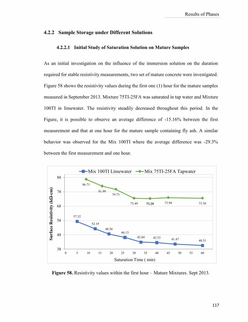
Results of Phases
117
4.2.2 Sample Storage under Different Solutions
4.2.2.1 Initial Study of Saturation Solution on Mature Samples
As an initial investigation on the influence of the immersion solution on the duration
required for stable resistivity measurements, two set of mature concrete were investigated.
Figure 58 shows the resistivity values during the first one (1) hour for the mature samples
measured in September 2013. Mixture 75TI-25FA was saturated in tap water and Mixture
100TI in limewater. The resistivity steadily decreased throughout this period. In the
Figure, it is possible to observe an average difference of -15.16% between the first
measurement and that at one hour for the mature sample containing fly ash. A similar
behavior was observed for the Mix 100TI where the average difference was -29.3%
between the first measurement and one hour.
57.32
52.19
48.5646.13
42.84 42.5341.47 40.51
86.71
81.9979.73
73.49 73.2973.29 73.94 73.56
38
48
58
68
78
88
0 5 10 15 20 25 30 35 40 45 50 55 60
Su
rfa
ce R
esis
tivit
y (
kΩ
-cm
)
Saturation Time ( min)
Mix 100TI Limewater Mix 75TI-25FA Tapwater
Figure 58. Resistivity values within the first hour – Mature Mixtures. Sept 2013.
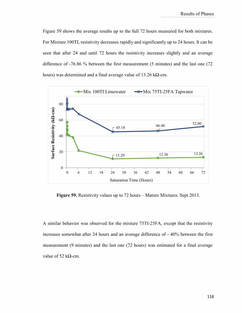
Results of Phases
118
Figure 59 shows the average results up to the full 72 hours measured for both mixtures.
For Mixture 100TI, resistivity decreases rapidly and significantly up to 24 hours. It can be
seen that after 24 and until 72 hours the resistivity increases slightly and an average
difference of -76.86 % between the first measurement (5 minutes) and the last one (72
hours) was determined and a final average value of 13.26 kΩ-cm.
Figure 59. Resistivity values up to 72 hours – Mature Mixtures. Sept 2013.
A similar behavior was observed for the mixture 75TI-25FA, except that the resistivity
increases somewhat after 24 hours and an average difference of - 40% between the first
measurement (9 minutes) and the last one (72 hours) was estimated for a final average
value of 52 kΩ-cm.
11.29 12.36 13.26
45.1846.40
52.00
0
20
40
60
80
0 6 12 18 24 30 36 42 48 54 60 66 72
Su
rfa
ce R
esis
tiv
ity
(k
Ω-c
m)
Saturation Time (Hours)
Mix 100TI Limewater Mix 75TI-25FA Tapwater
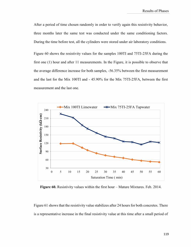
Results of Phases
119
After a period of time chosen randomly in order to verify again this resistivity behavior,
three months later the same test was conducted under the same conditioning factors.
During the time before test, all the cylinders were stored under air laboratory conditions.
Figure 60 shows the resistivity values for the samples 100TI and 75TI-25FA during the
first one (1) hour and after 11 measurements. In the Figure, it is possible to observe that
the average difference increase for both samples, -56.35% between the first measurement
and the last for the Mix 100TI and - 45.90% for the Mix 75TI-25FA, between the first
measurement and the last one.
Figure 61 shows that the resistivity value stabilizes after 24 hours for both concretes. There
is a representative increase in the final resistivity value at this time after a small period of
30
60
90
120
150
180
210
240
0 5 10 15 20 25 30 35 40 45 50 55 60
Su
rface
Res
isti
vit
y (
kΩ
-cm
)
Saturation Time ( min)
Mix 100TI Limewater Mix 75TI-25FA Tapwater
Figure 60. Resistivity values within the first hour – Mature Mixtures. Feb. 2014.
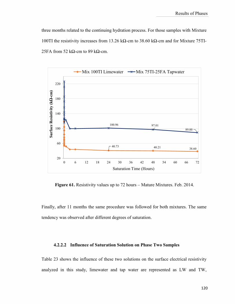
Results of Phases
120
three months related to the continuing hydration process. For those samples with Mixture
100TI the resistivity increases from 13.26 kΩ-cm to 38.60 kΩ-cm and for Mixture 75TI-
25FA from 52 kΩ-cm to 89 kΩ-cm.
Figure 61. Resistivity values up to 72 hours – Mature Mixtures. Feb. 2014.
Finally, after 11 months the same procedure was followed for both mixtures. The same
tendency was observed after different degrees of saturation.
4.2.2.2 Influence of Saturation Solution on Phase Two Samples
Table 23 shows the influence of these two solutions on the surface electrical resistivity
analyzed in this study, limewater and tap water are represented as LW and TW,
40.73 40.21 38.60
100.96 97.01
89.00
20
60
100
140
180
220
0 6 12 18 24 30 36 42 48 54 60 66 72
Su
rface
Res
isti
vit
y (
kΩ
-cm
)
Saturation Time (Hours)
Mix 100TI Limewater Mix 75TI-25FA Tapwater
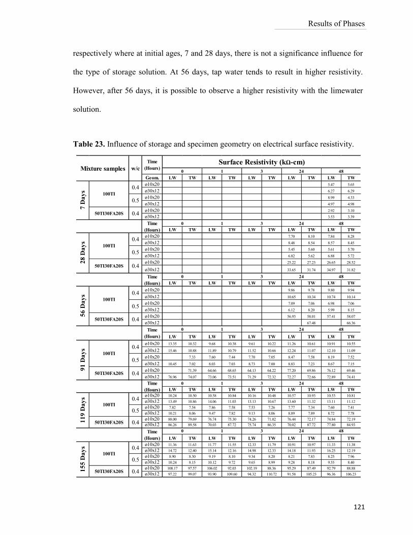
Results of Phases
121
respectively where at initial ages, 7 and 28 days, there is not a significance influence for
the type of storage solution. At 56 days, tap water tends to result in higher resistivity.
However, after 56 days, it is possible to observe a higher resistivity with the limewater
solution.
Table 23. Influence of storage and specimen geometry on electrical surface resistivity.
Geom. LW TW LW TW LW TW LW TW LW TW
ø10x20 5.47 5.65
ø30x12 6.27 6.29
ø10x20 8.99 4.33
ø30x12 4.97 4.98
ø10x20 2.92 3.10
ø30x12 3.53 3.39
LW TW LW TW LW TW LW TW LW TW
ø10x20 7.70 8.10 7.84 8.28
ø30x12 8.48 8.54 8.57 8.45
ø10x20 5.45 5.60 5.61 5.70
ø30x12 6.82 5.62 6.88 5.72
ø10x20 25.22 27.23 26.65 28.52
ø30x12 33.65 31.74 34.97 31.82
LW TW LW TW LW TW LW TW LW TW
ø10x20 9.86 9.78 9.80 9.94
ø30x12 10.65 10.34 10.74 10.14
ø10x20 7.09 7.06 6.98 7.06
ø30x12 6.12 8.20 5.99 8.15
ø10x20 56.93 58.01 57.41 58.07
ø30x12 67.48 66.36
LW TW LW TW LW TW LW TW LW TW
ø10x20 13.35 10.32 9.68 10.38 9.61 10.22 11.26 10.61 10.91 10.55
ø30x12 15.46 10.88 11.89 10.79 11.52 10.66 12.24 11.07 12.10 11.09
ø10x20 7.33 7.60 7.44 7.70 7.05 8.47 7.58 8.19 7.52
ø30x12 10.45 7.02 8.03 7.03 8.73 7.00 8.83 7.23 8.67 7.15
ø10x20 71.39 64.66 68.65 64.13 64.22 77.20 69.86 76.12 69.46
ø30x12 76.96 74.07 73.06 73.51 71.29 72.32 72.27 72.66 72.89 74.41
LW TW LW TW LW TW LW TW LW TW
ø10x20 10.24 10.50 10.58 10.84 10.16 10.48 10.57 10.93 10.53 10.81
ø30x12 13.49 10.86 14.06 11.03 13.13 10.67 13.60 11.32 13.11 11.12
ø10x20 7.82 7.54 7.86 7.58 7.53 7.26 7.77 7.34 7.60 7.41
ø30x12 10.21 8.06 9.47 7.82 9.13 8.06 8.89 7.89 8.72 7.78
ø10x20 88.00 79.69 76.74 75.30 74.26 71.02 76.44 72.17 74.84 72.19
ø30x12 86.26 89.58 70.03 87.72 75.74 86.35 70.02 87.72 77.80 84.93
LW TW LW TW LW TW LW TW LW TW
ø10x20 11.36 11.63 11.77 11.55 12.33 11.79 10.91 10.97 11.33 11.38
ø30x12 14.72 12.40 15.14 12.16 14.98 12.33 14.18 11.93 16.25 12.19
ø10x20 8.90 8.30 9.19 8.10 9.34 8.20 8.21 7.83 8.25 7.96
ø30x12 10.24 8.15 10.12 9.72 9.65 8.99 9.28 8.18 9.55 8.40
ø10x20 108.17 97.57 106.02 92.03 102.19 88.36 95.29 87.49 92.79 88.88
ø30x12 97.22 99.07 93.90 109.60 94.32 110.72 91.58 105.23 96.36 106.23
50TI30FA20S 0.4
Mixture samples w/c
Time
(Hours)Surface Resistivity (kΩ-cm)
0 1 3 24 48
Time
(Hours)
0 1 3 24 48
7 D
ay
s
100TI
0.4
0.5
Time
(Hours)
0 1 3 24 48
28
Da
ys
100TI
0.4
0.5
50TI30FA20S 0.4
56
Da
ys
100TI
0.4
0.5
50TI30FA20S 0.4
91
Da
ys
100TI
0.4
50TI30FA20S
Time
(Hours)
0 1 3 24 48
0.5
0.4
11
9 D
ay
s
100TI
0.4
0.5
50TI30FA20S 0.4
Time
(Hours)
0 1 3 24 48
15
5 D
ay
s
100TI
0.4
0.5
50TI30FA20S 0.4
Time
(Hours)
0 1 3 24 48
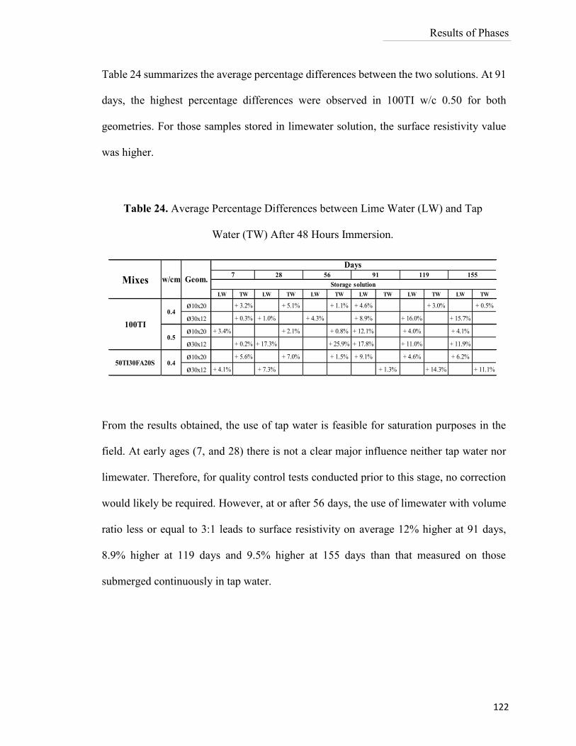
Results of Phases
122
Table 24 summarizes the average percentage differences between the two solutions. At 91
days, the highest percentage differences were observed in 100TI w/c 0.50 for both
geometries. For those samples stored in limewater solution, the surface resistivity value
was higher.
From the results obtained, the use of tap water is feasible for saturation purposes in the
field. At early ages (7, and 28) there is not a clear major influence neither tap water nor
limewater. Therefore, for quality control tests conducted prior to this stage, no correction
would likely be required. However, at or after 56 days, the use of limewater with volume
ratio less or equal to 3:1 leads to surface resistivity on average 12% higher at 91 days,
8.9% higher at 119 days and 9.5% higher at 155 days than that measured on those
submerged continuously in tap water.
LW TW LW TW LW TW LW TW LW TW LW TW
ø10x20 + 3.2% + 5.1% + 1.1% + 4.6% + 3.0% + 0.5%
ø30x12 + 0.3% + 1.0% + 4.3% + 8.9% + 16.0% + 15.7%
ø10x20 + 3.4% + 2.1% + 0.8% + 12.1% + 4.0% + 4.1%
ø30x12 + 0.2% + 17.3% + 25.9% + 17.8% + 11.0% + 11.9%
ø10x20 + 5.6% + 7.0% + 1.5% + 9.1% + 4.6% + 6.2%
ø30x12 + 4.1% + 7.3% + 1.3% + 14.3% + 11.1%
0.5
50TI30FA20S 0.4
56 91 119 155
Storage solution
100TI
0.4
Mixes w/cm Geom.
Days 7 28
Table 24. Average Percentage Differences between Lime Water (LW) and Tap
Water (TW) After 48 Hours Immersion.
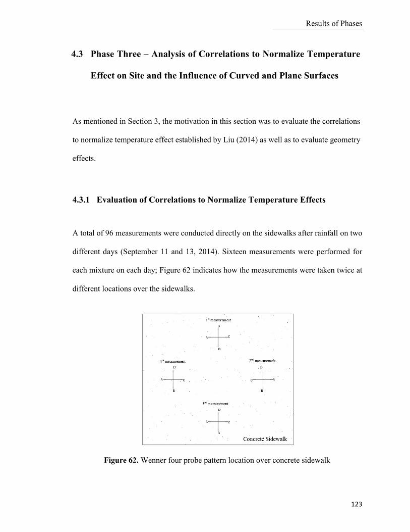
Results of Phases
123
4.3 Phase Three – Analysis of Correlations to Normalize Temperature
Effect on Site and the Influence of Curved and Plane Surfaces
As mentioned in Section 3, the motivation in this section was to evaluate the correlations
to normalize temperature effect established by Liu (2014) as well as to evaluate geometry
effects.
4.3.1 Evaluation of Correlations to Normalize Temperature Effects
A total of 96 measurements were conducted directly on the sidewalks after rainfall on two
different days (September 11 and 13, 2014). Sixteen measurements were performed for
each mixture on each day; Figure 62 indicates how the measurements were taken twice at
different locations over the sidewalks.
Figure 62. Wenner four probe pattern location over concrete sidewalk
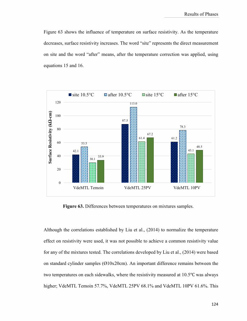
Results of Phases
124
Figure 63 shows the influence of temperature on surface resistivity. As the temperature
decreases, surface resistivity increases. The word “site” represents the direct measurement
on site and the word “after” means, after the temperature correction was applied, using
equations 15 and 16.
Although the correlations established by Liu et al., (2014) to normalize the temperature
effect on resistivity were used, it was not possible to achieve a common resistivity value
for any of the mixtures tested. The correlations developed by Liu et al., (2014) were based
on standard cylinder samples (Ø10x20cm). An important difference remains between the
two temperatures on each sidewalks, where the resistivity measured at 10.5 was always
higher; VdeMTL Temoin 57.7%, VdeMTL 25PV 68.1% and VdeMTL 10PV 61.6%. This
42.1
87.5
61.2
53.5
113.0
78.3
30.1
61.4
43.1
33.9
67.2
48.5
0
20
40
60
80
100
120
VdeMTL Temoin VdeMTL 25PV VdeMTL 10PV
Su
rface
Res
isti
vit
y (
kΩ
-cm
)
site 10.5°C after 10.5°C site 15°C after 15°C
Figure 63. Differences between temperatures on mixtures samples.
Results of Phases
125
difference may be related to lack of full saturation. On site it was not possible to measure
the saturation level on each sidewalk. A sense of the depth of water penetration and the
uniformity of the water absorption was not possible to verify. Another factor may be the
difference between curved and plane surfaces as seen in this research (as shown in section
4.2.1).
4.3.2 Differences between Curved and Plane Surfaces
On site, the dimensions of concrete elements being studied on site are large in comparison
to the Wenner four probe electrodes spacing 𝑎, so it is possible to have the assumption that
the current passes through a semi-infinite plane rather than a restricted and curved plane
(Chun-Tao et al., 2014). Commonly most of the onsite measurements take place on planar
surfaces, (bridge desks, beams, PCC pavements, etc.). For this reason, the determination
of the onsite surface resistivity by cylinders generates a level of uncertainty. The
motivation in this section was evaluating the resistivity differences on cylinders specimens
(Ø10x20cm and Ø15x30cm) with curved surfaces against plane surfaces (sidewalks) with
the same mixture properties.
The differences found between planar and curved surfaces can be seen in Figures 65, 66,
and 67. All the values obtained for the cylinder samples were corrected using the geometry
factor (k = 1.89 for cylinders Ø10x20cm, k = 1.39 for cylinders Ø15x30cm). The “Conc.
Sidewalk” label represents the measurement made on site on the planar surfaces at the two
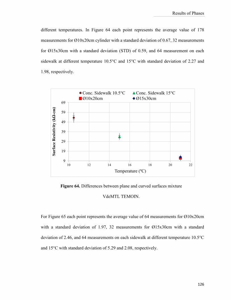
Results of Phases
126
different temperatures. In Figure 64 each point represents the average value of 178
measurements for Ø10x20cm cylinder with a standard deviation of 0.67, 32 measurements
for Ø15x30cm with a standard deviation (STD) of 0.59, and 64 measurement on each
sidewalk at different temperature 10.5°C and 15°C with standard deviation of 2.27 and
1.98, respectively.
For Figure 65 each point represents the average value of 64 measurements for Ø10x20cm
with a standard deviation of 1.97, 32 measurements for Ø15x30cm with a standard
deviation of 2.46, and 64 measurements on each sidewalk at different temperature 10.5°C
and 15°C with standard deviation of 5.29 and 2.08, respectively.
9
19
29
39
49
59
69
10 12 14 16 18 20 22
Su
rface
Res
isti
vit
y (
kΩ
-cm
)
Temperature (ºC)
Conc. Sidewalk 10.5°C Conc. Sidewalk 15°C
Ø10x20cm Ø15x30cm
Figure 64. Differences between plane and curved surfaces mixture
VdeMTL TEMOIN.
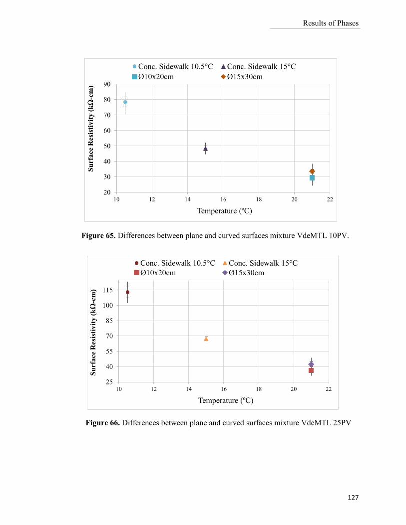
Results of Phases
127
25
40
55
70
85
100
115
10 12 14 16 18 20 22
Su
rfa
ce R
esis
tivit
y (
kΩ
-cm
)
Temperature (ºC)
Conc. Sidewalk 10.5°C Conc. Sidewalk 15°C
Ø10x20cm Ø15x30cm
Figure 66. Differences between plane and curved surfaces mixture VdeMTL 25PV
20
30
40
50
60
70
80
90
10 12 14 16 18 20 22
Su
rface
Res
isti
vit
y (
kΩ
-cm
)
Temperature (ºC)
Conc. Sidewalk 10.5°C Conc. Sidewalk 15°C
Ø10x20cm Ø15x30cm
Figure 65. Differences between plane and curved surfaces mixture VdeMTL 10PV.
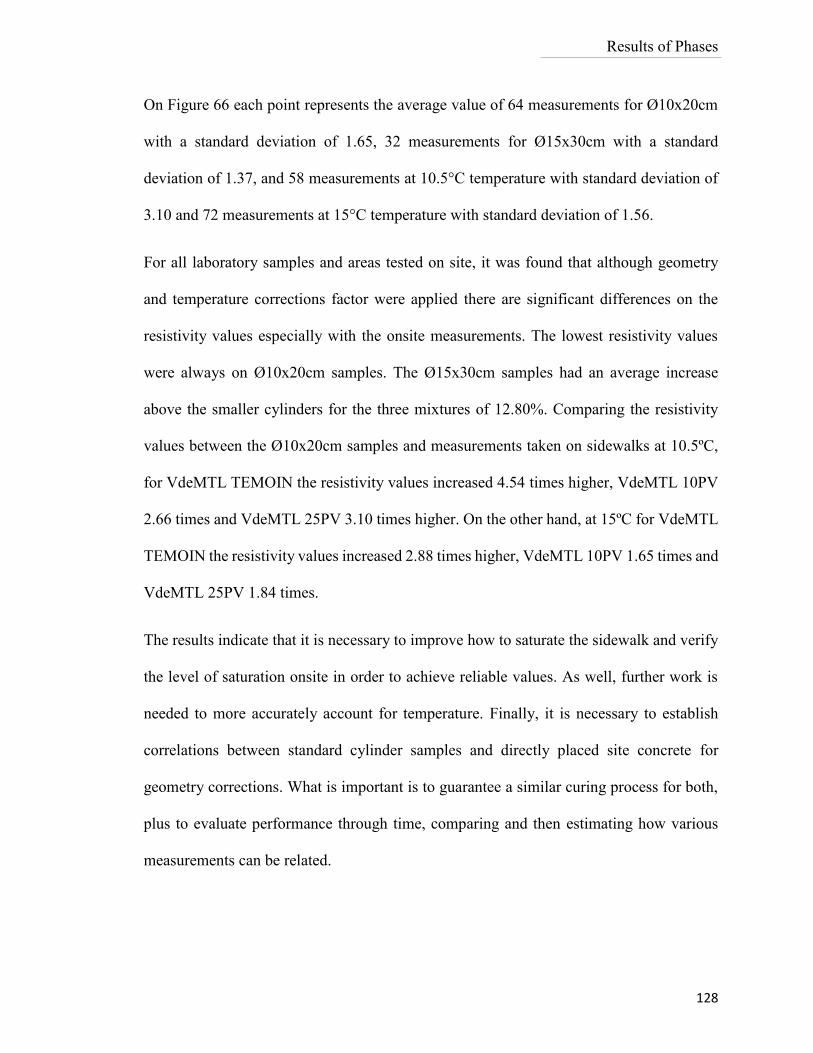
Results of Phases
128
On Figure 66 each point represents the average value of 64 measurements for Ø10x20cm
with a standard deviation of 1.65, 32 measurements for Ø15x30cm with a standard
deviation of 1.37, and 58 measurements at 10.5°C temperature with standard deviation of
3.10 and 72 measurements at 15°C temperature with standard deviation of 1.56.
For all laboratory samples and areas tested on site, it was found that although geometry
and temperature corrections factor were applied there are significant differences on the
resistivity values especially with the onsite measurements. The lowest resistivity values
were always on Ø10x20cm samples. The Ø15x30cm samples had an average increase
above the smaller cylinders for the three mixtures of 12.80%. Comparing the resistivity
values between the Ø10x20cm samples and measurements taken on sidewalks at 10.5ºC,
for VdeMTL TEMOIN the resistivity values increased 4.54 times higher, VdeMTL 10PV
2.66 times and VdeMTL 25PV 3.10 times higher. On the other hand, at 15ºC for VdeMTL
TEMOIN the resistivity values increased 2.88 times higher, VdeMTL 10PV 1.65 times and
VdeMTL 25PV 1.84 times.
The results indicate that it is necessary to improve how to saturate the sidewalk and verify
the level of saturation onsite in order to achieve reliable values. As well, further work is
needed to more accurately account for temperature. Finally, it is necessary to establish
correlations between standard cylinder samples and directly placed site concrete for
geometry corrections. What is important is to guarantee a similar curing process for both,
plus to evaluate performance through time, comparing and then estimating how various
measurements can be related.
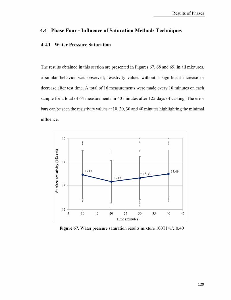
Results of Phases
129
4.4 Phase Four - Influence of Saturation Methods Techniques
4.4.1 Water Pressure Saturation
The results obtained in this section are presented in Figures 67, 68 and 69. In all mixtures,
a similar behavior was observed; resistivity values without a significant increase or
decrease after test time. A total of 16 measurements were made every 10 minutes on each
sample for a total of 64 measurements in 40 minutes after 125 days of casting. The error
bars can be seen the resistivity values at 10, 20, 30 and 40 minutes highlighting the minimal
influence.
13.47
13.17
13.3313.49
12
13
14
15
5 10 15 20 25 30 35 40 45
Su
rfa
ce r
esi
stiv
ity
(k
Ω-c
m)
Time (minutes)
Figure 67. Water pressure saturation results mixture 100TI w/c 0.40
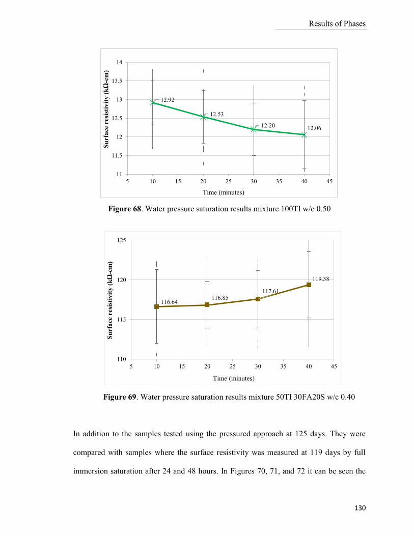
Results of Phases
130
In addition to the samples tested using the pressured approach at 125 days. They were
compared with samples where the surface resistivity was measured at 119 days by full
immersion saturation after 24 and 48 hours. In Figures 70, 71, and 72 it can be seen the
Figure 68. Water pressure saturation results mixture 100TI w/c 0.50
116.64116.85
117.61
119.38
110
115
120
125
5 10 15 20 25 30 35 40 45
Su
rfa
ce r
esi
stiv
ity
(k
Ω-c
m)
Time (minutes)
Figure 69. Water pressure saturation results mixture 50TI 30FA20S w/c 0.40
12.92
12.53
12.20 12.06
11
11.5
12
12.5
13
13.5
14
5 10 15 20 25 30 35 40 45
Su
rfa
ce r
esi
stiv
ity
(k
Ω-c
m)
Time (minutes)
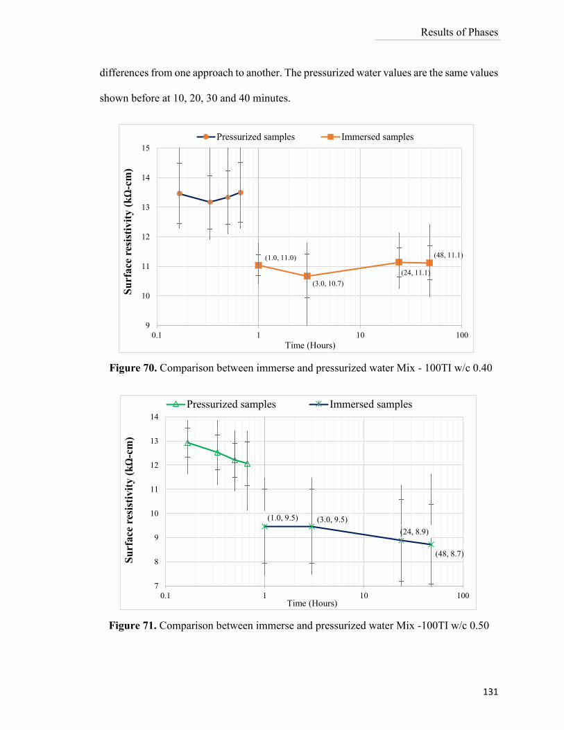
Results of Phases
131
differences from one approach to another. The pressurized water values are the same values
shown before at 10, 20, 30 and 40 minutes.
Figure 70. Comparison between immerse and pressurized water Mix - 100TI w/c 0.40
Figure 71. Comparison between immerse and pressurized water Mix -100TI w/c 0.50
(1.0, 11.0)
(3.0, 10.7)
(24, 11.1)
(48, 11.1)
9
10
11
12
13
14
15
0.1 1 10 100
Su
rface
res
isti
vit
y (
kΩ
-cm
)
Time (Hours)
Pressurized samples Immersed samples
(1.0, 9.5) (3.0, 9.5)
(24, 8.9)
(48, 8.7)
7
8
9
10
11
12
13
14
0.1 1 10 100
Su
rface
res
isti
vit
y (
kΩ
-cm
)
Time (Hours)
Pressurized samples Immersed samples
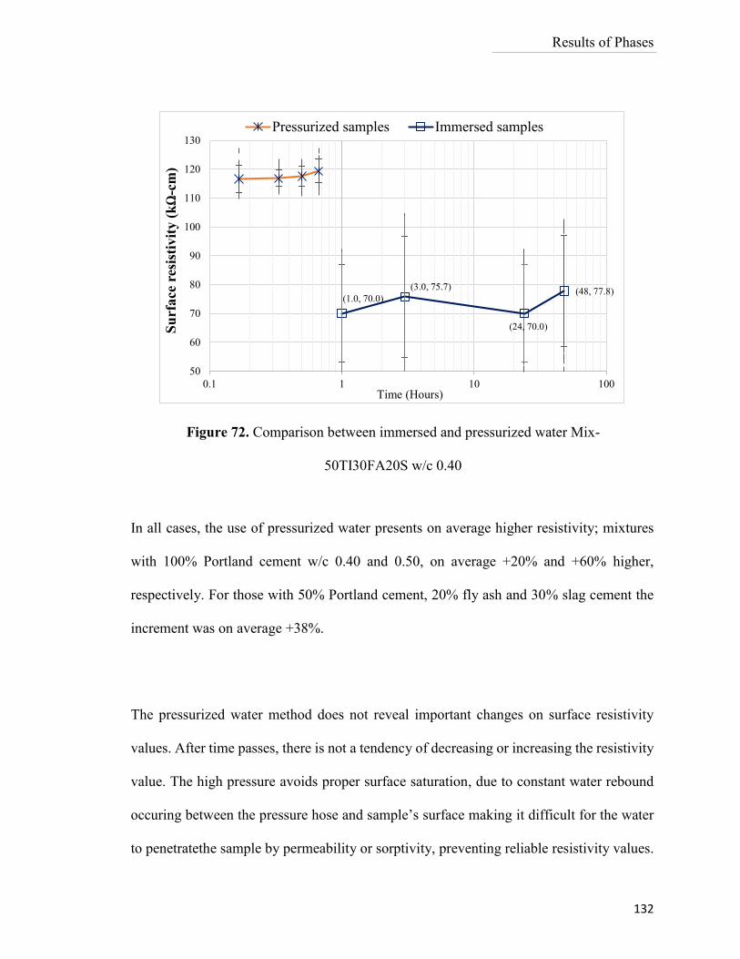
Results of Phases
132
In all cases, the use of pressurized water presents on average higher resistivity; mixtures
with 100% Portland cement w/c 0.40 and 0.50, on average +20% and +60% higher,
respectively. For those with 50% Portland cement, 20% fly ash and 30% slag cement the
increment was on average +38%.
The pressurized water method does not reveal important changes on surface resistivity
values. After time passes, there is not a tendency of decreasing or increasing the resistivity
value. The high pressure avoids proper surface saturation, due to constant water rebound
occuring between the pressure hose and sample’s surface making it difficult for the water
to penetratethe sample by permeability or sorptivity, preventing reliable resistivity values.
Figure 72. Comparison between immersed and pressurized water Mix-
50TI30FA20S w/c 0.40
(1.0, 70.0)
(3.0, 75.7)
(24, 70.0)
(48, 77.8)
50
60
70
80
90
100
110
120
130
0.1 1 10 100
Su
rface
res
isti
vit
y (
kΩ
-cm
)
Time (Hours)
Pressurized samples Immersed samples
Results of Phases
133
Additionally, the amount of discharge water used during the test is excessively high making
this approach difficult to implement in construction projects without water facilities.
4.4.2 Ponding Saturation
After the last testing at 155 days, all the circular slabs from Phase Two mixtures were
stored in laboratory air conditions for 50 days to achieve a dry sample at 205 days. For
periods of time (10, 30 and 60 minutes) the samples were surface saturated (by ponding
with tap water) to simulate on site practices. After the resistivity measurements were
completed, the slabs were fully immersed in tap-water for 72 hours. Surface resistivity was
measured at 24, 48 and 72 hours of immersion. A total of nine samples were measured,
three samples of each mixture. In all cases, an important decrease was observed in the
surface resistivity between the first measurements at 10 minutes with the last one at 72
hours.
Figures 73, 74 and 75 shows the generalized decreasing behavior observed using ponding
saturation. Each point represents the average results of 16 measurements at every time (10,
30, and 60 minute, 24, 48 and 72 hours) on each sample. The “x” axis is in a logarithmic
scale in order to facilitate the view of measurements at 10 min and 30 min.
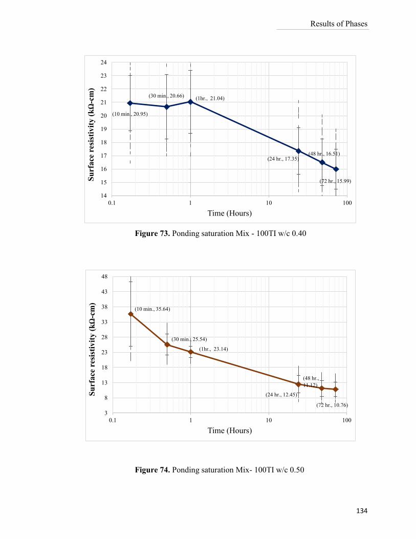
Results of Phases
134
Figure 74. Ponding saturation Mix- 100TI w/c 0.50
14
15
16
17
18
19
20
21
22
23
24
0.1 1 10 100
Su
rface
res
isti
vit
y (
kΩ
-cm
)
Time (Hours)
(10 min., 20.95)
(30 min., 20.66)(1hr., 21.04)
(24 hr., 17.35)(48 hr., 16.51)
(72 hr., 15.99)
3
8
13
18
23
28
33
38
43
48
0.1 1 10 100
Su
rface
res
isti
vit
y (
kΩ
-cm
)
Time (Hours)
(10 min., 35.64)
(30 min., 25.54)
(1hr., 23.14)
(24 hr., 12.45)
(48 hr.,
11.12)
(72 hr., 10.76)
Figure 73. Ponding saturation Mix - 100TI w/c 0.40
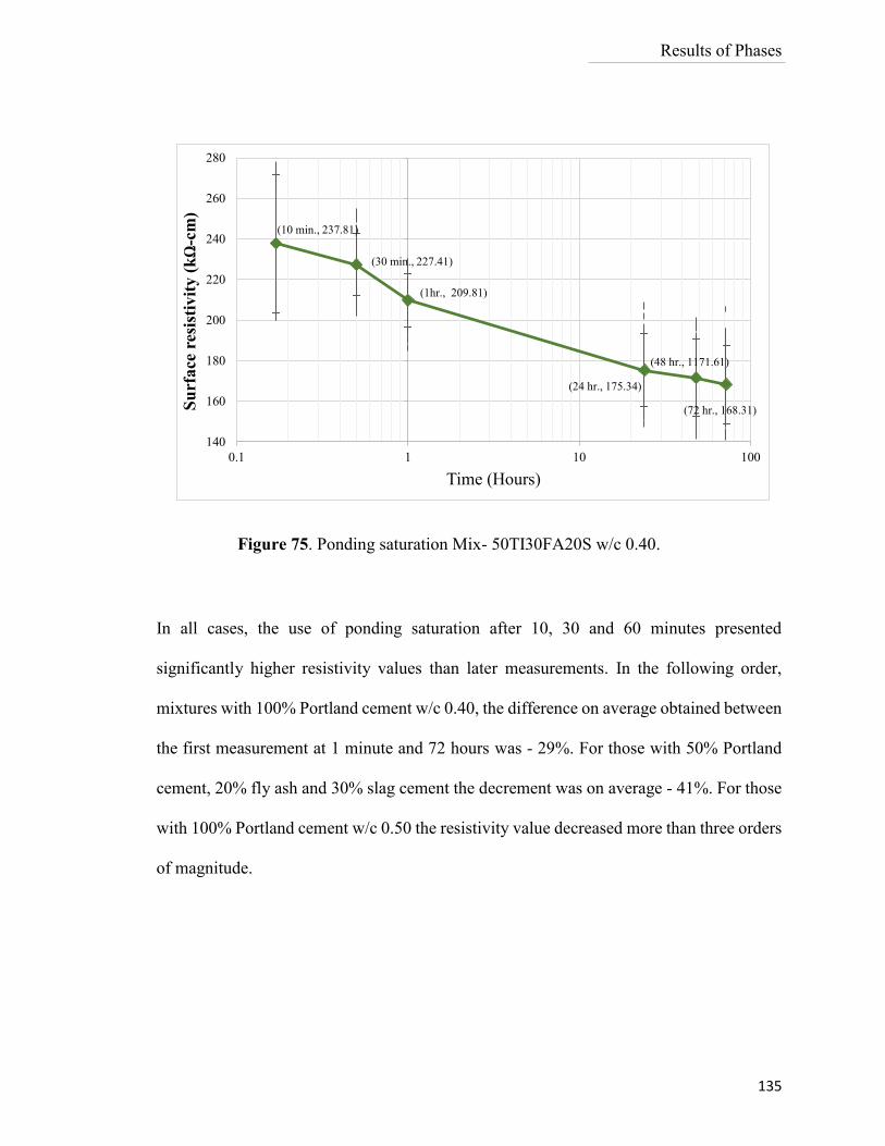
Results of Phases
135
In all cases, the use of ponding saturation after 10, 30 and 60 minutes presented
significantly higher resistivity values than later measurements. In the following order,
mixtures with 100% Portland cement w/c 0.40, the difference on average obtained between
the first measurement at 1 minute and 72 hours was - 29%. For those with 50% Portland
cement, 20% fly ash and 30% slag cement the decrement was on average - 41%. For those
with 100% Portland cement w/c 0.50 the resistivity value decreased more than three orders
of magnitude.
Figure 75. Ponding saturation Mix- 50TI30FA20S w/c 0.40.
140
160
180
200
220
240
260
280
0.1 1 10 100
Su
rface
res
isti
vit
y (
kΩ
-cm
)
Time (Hours)
(10 min., 237.81)
(30 min., 227.41)
(1hr., 209.81)
(24 hr., 175.34)
(48 hr., 1171.61)
(72 hr., 168.31)
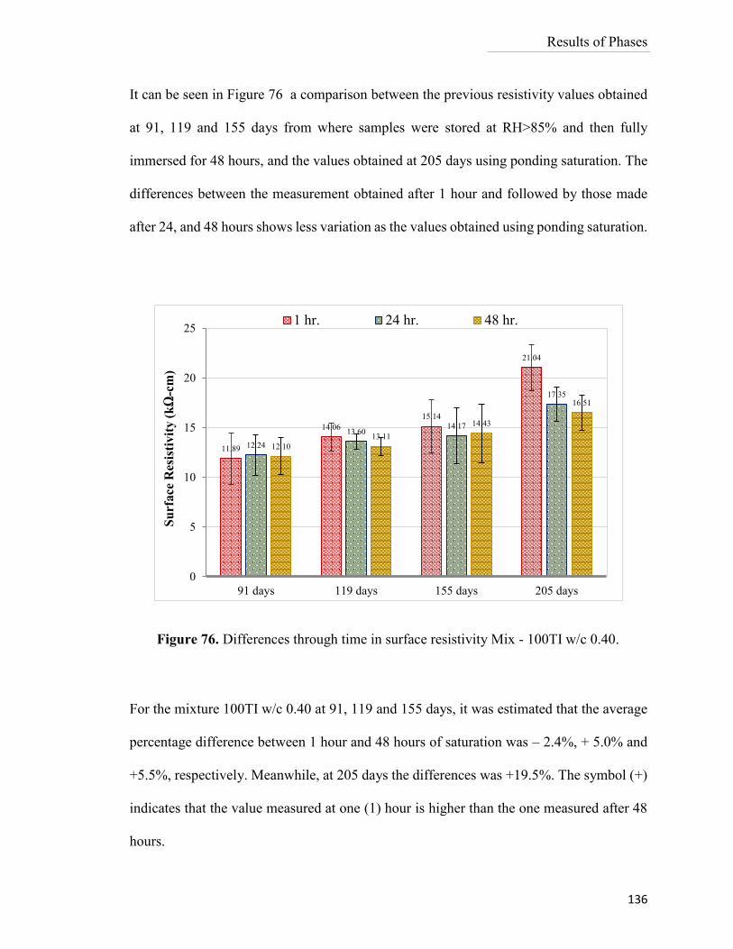
Results of Phases
136
It can be seen in Figure 76 a comparison between the previous resistivity values obtained
at 91, 119 and 155 days from where samples were stored at RH>85% and then fully
immersed for 48 hours, and the values obtained at 205 days using ponding saturation. The
differences between the measurement obtained after 1 hour and followed by those made
after 24, and 48 hours shows less variation as the values obtained using ponding saturation.
For the mixture 100TI w/c 0.40 at 91, 119 and 155 days, it was estimated that the average
percentage difference between 1 hour and 48 hours of saturation was – 2.4%, + 5.0% and
+5.5%, respectively. Meanwhile, at 205 days the differences was +19.5%. The symbol (+)
indicates that the value measured at one (1) hour is higher than the one measured after 48
hours.
Figure 76. Differences through time in surface resistivity Mix - 100TI w/c 0.40.
11.89
14.06
15.14
21.04
12.24
13.6014.17
17.35
12.10
13.11
14.43
16.51
0
5
10
15
20
25
91 days 119 days 155 days 205 days
Su
rface
Res
isti
vit
y (
kΩ
-cm
)
1 hr. 24 hr. 48 hr.
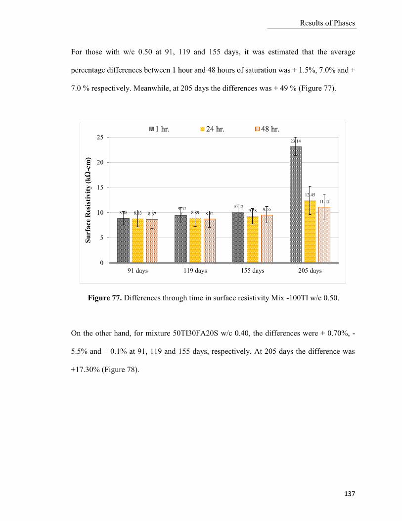
Results of Phases
137
For those with w/c 0.50 at 91, 119 and 155 days, it was estimated that the average
percentage differences between 1 hour and 48 hours of saturation was + 1.5%, 7.0% and +
7.0 % respectively. Meanwhile, at 205 days the differences was + 49 % (Figure 77).
On the other hand, for mixture 50TI30FA20S w/c 0.40, the differences were + 0.70%, -
5.5% and – 0.1% at 91, 119 and 155 days, respectively. At 205 days the difference was
+17.30% (Figure 78).
Figure 77. Differences through time in surface resistivity Mix -100TI w/c 0.50.
8.889.47 10.12
23.14
8.83 8.89 9.28
12.45
8.67 8.729.55
11.12
0
5
10
15
20
25
91 days 119 days 155 days 205 days
Su
rface
Res
isti
vit
y (
kΩ
-cm
)
1 hr. 24 hr. 48 hr.
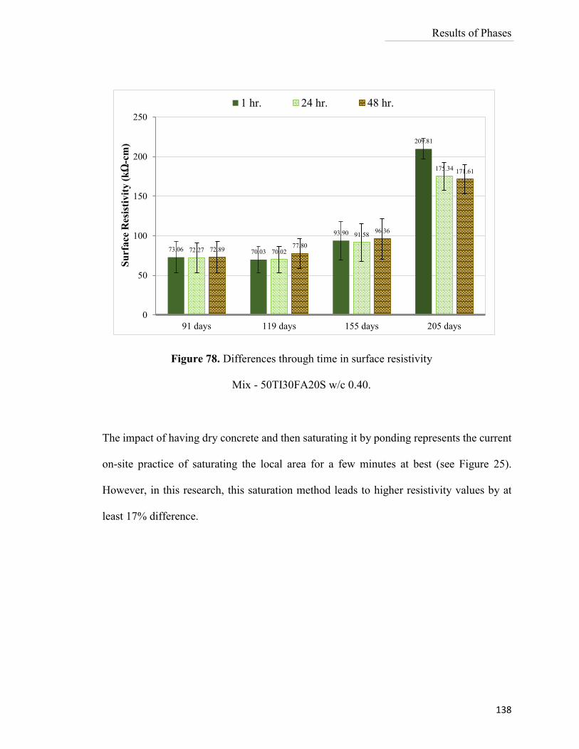
Results of Phases
138
The impact of having dry concrete and then saturating it by ponding represents the current
on-site practice of saturating the local area for a few minutes at best (see Figure 25).
However, in this research, this saturation method leads to higher resistivity values by at
least 17% difference.
Figure 78. Differences through time in surface resistivity
Mix - 50TI30FA20S w/c 0.40.
73.06 70.03
93.90
209.81
72.27 70.02
91.58
175.34
72.8977.80
96.36
171.61
0
50
100
150
200
250
91 days 119 days 155 days 205 days
Su
rface
Res
isti
vit
y (
kΩ
-cm
)
1 hr. 24 hr. 48 hr.
139
5 Discussion
This Chapter further discusses the results comparing outcomes among the phases. There
are some limitations regarding this research, such as:
For all the Surface resistivity measurements at different ages, samples were stored
under the same laboratory conditions, RH>85%. Once the measurements started
they were immersed in limewater or tap water according the case. The results are
expected to be similar for other starting saturation, but this conclusion should be
verified.
In all cases, only one variable was analyzed at the time against surface electrical
resistivity (i.e. saturation time vs. surface electrical resistivity). On site more than
one variable can influence surface electrical measurements at the same time (i.e.
temperature, saturation time, moisture degree, type of surface, etc.).
This section discusses three main topics; (a) the minimum duration to obtain reliable
surface resistivity values on laboratory samples; (b) Geometry effect and type of solution
for saturation; (c) misreading surface electrical resistivity results due to poor saturation
based on results achieved in Chapter 4.
Discussion
140
5.1 Minimum Duration Time to Achieve Reliable Surface Resistivity
Values
A comparison between the samples with equal or similar water cement ratio (w/c) was
established with different geometry and mixture properties from Phases One and Two.
The surface resistivity was compared at different times 28, 56 and 91 days for standard
cylinders Ø10x20cm and at 91, 119 and 155 days for circular slabs Ø30x12cm to identify
the percentage difference in surface resistivity between samples partially saturated (after
only hour) and fully saturated for 24 and 72 hours of fully immersion into limewater but
stored before testing at RH >85%.
5.1.1 Differences on Resistivity values in Standard Cylinders Ø10x20cm
As can be seen in Figure 79 the resistivity for all the samples with water cement ratio close
to 0.40 at 28 days is given. The mixture with major differences between first measurement
(1 hour saturation) and measurements at 24 and 72 hours were for those with only Portland
cement (100TI) with -7.86% and -9.60%, followed by the mixture 50TI-30FA-20S with
differences of -7.36% and - 3.0% at 24 and 72 hours. For mixtures 50L50S and 50TI-
20FA-30S the resistivity value obtained after 72 hours surpass the one obtained at the first
measurement by +3.0% and +12.40% respectively.
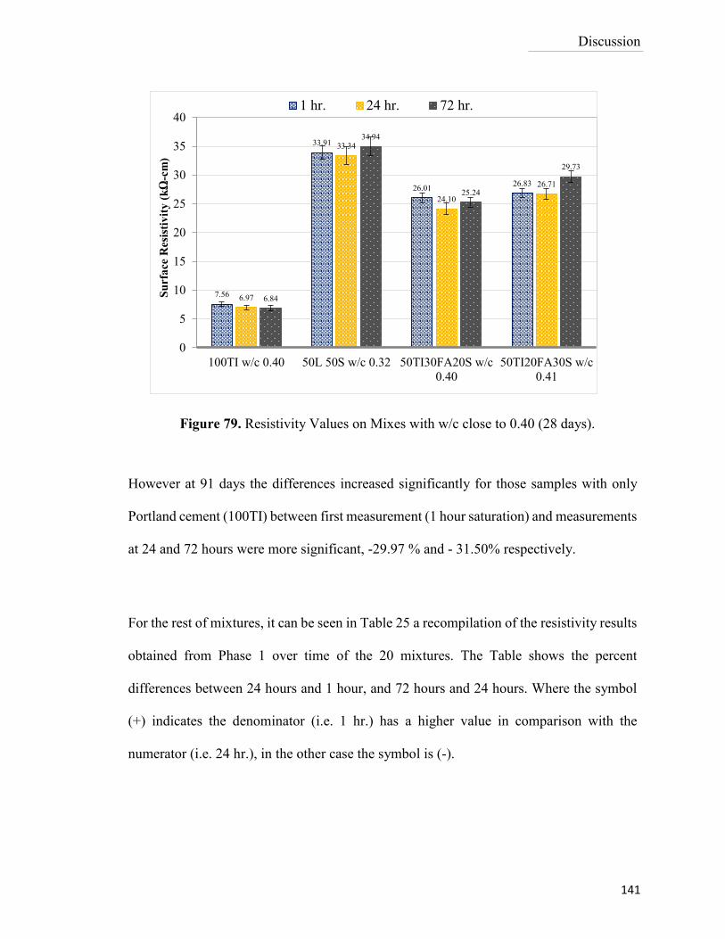
Discussion
141
However at 91 days the differences increased significantly for those samples with only
Portland cement (100TI) between first measurement (1 hour saturation) and measurements
at 24 and 72 hours were more significant, -29.97 % and - 31.50% respectively.
For the rest of mixtures, it can be seen in Table 25 a recompilation of the resistivity results
obtained from Phase 1 over time of the 20 mixtures. The Table shows the percent
differences between 24 hours and 1 hour, and 72 hours and 24 hours. Where the symbol
(+) indicates the denominator (i.e. 1 hr.) has a higher value in comparison with the
numerator (i.e. 24 hr.), in the other case the symbol is (-).
7.56
33.91
26.0126.83
6.97
33.34
24.10
26.71
6.84
34.94
25.24
29.73
0
5
10
15
20
25
30
35
40
100TI w/c 0.40 50L 50S w/c 0.32 50TI30FA20S w/c
0.40
50TI20FA30S w/c
0.41
Su
rfa
ce R
esis
tiv
ity
(k
Ω-c
m)
1 hr. 24 hr. 72 hr.
Figure 79. Resistivity Values on Mixes with w/c close to 0.40 (28 days).
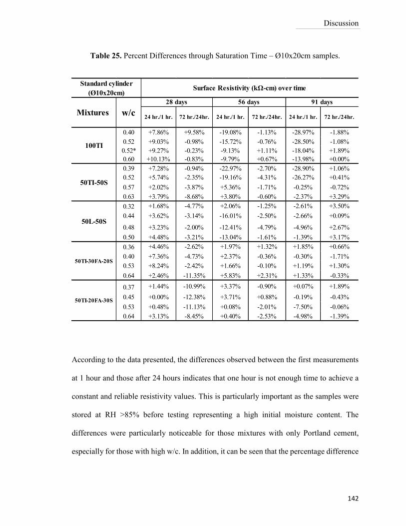
Discussion
142
Table 25. Percent Differences through Saturation Time – Ø10x20cm samples.
According to the data presented, the differences observed between the first measurements
at 1 hour and those after 24 hours indicates that one hour is not enough time to achieve a
constant and reliable resistivity values. This is particularly important as the samples were
stored at RH >85% before testing representing a high initial moisture content. The
differences were particularly noticeable for those mixtures with only Portland cement,
especially for those with high w/c. In addition, it can be seen that the percentage difference
0.40 +7.86% +9.58% -19.08% -1.13% -28.97% -1.88%
0.52 +9.03% -0.98% -15.72% -0.76% -28.50% -1.08%
0.52* +9.27% -0.23% -9.13% +1.11% -18.04% +1.89%
0.60 +10.13% -0.83% -9.79% +0.67% -13.98% +0.00%
0.39 +7.28% -0.94% -22.97% -2.70% -28.90% +1.06%
0.52 +5.74% -2.35% -19.16% -4.31% -26.27% +0.41%
0.57 +2.02% -3.87% +5.36% -1.71% -0.25% -0.72%
0.63 +3.79% -8.68% +3.80% -0.60% -2.37% +3.29%
0.32 +1.68% -4.77% +2.06% -1.25% -2.61% +3.50%
0.44 +3.62% -3.14% -16.01% -2.50% -2.66% +0.09%
0.48 +3.23% -2.00% -12.41% -4.79% -4.96% +2.67%
0.50 +4.48% -3.21% -13.04% -1.61% -1.39% +3.17%
0.36 +4.46% -2.62% +1.97% +1.32% +1.85% +0.66%
0.40 +7.36% -4.73% +2.37% -0.36% -0.30% -1.71%
0.53 +8.24% -2.42% +1.66% -0.10% +1.19% +1.30%
0.64 +2.46% -11.35% +5.83% +2.31% +1.33% -0.33%
0.37 +1.44% -10.99% +3.37% -0.90% +0.07% +1.89%
0.45 +0.00% -12.38% +3.71% +0.88% -0.19% -0.43%
0.53 +0.48% -11.13% +0.08% -2.01% -7.50% -0.06%
0.64 +3.13% -8.45% +0.40% -2.53% -4.98% -1.39%
100TI
50TI-50S
w/cMixtures
Standard cylinder
(Ø10x20cm)Surface Resistivity (kΩ-cm) over time
28 days 56 days 91 days
24 hr./1 hr. 72 hr./24hr. 24 hr./1 hr. 72 hr./24hr. 24 hr./1 hr. 72 hr./24hr.
50L-50S
50TI-30FA-20S
50TI-20FA-30S
Discussion
143
between 24 and 72 hours for the same mixtures is generally less than or equal to 1.0% at
all ages.
For those blends with only two cementitious materials, 50TI-50S and 50L-50S a similar
behavior as for those with only Portland cement was achieved especially for those with a
w/c closer to 0.50 at 56 days and later. For those blends with three cementitious materials,
Portland cement, fly Ash and slag, the percent differences are very small and in some cases
not to seem important. However, to be conservative, 24 hours saturation results in stable
surface resistivity measurements.
5.1.2 Differences on Resistivity values in Circular Slabs Ø30x12cm
Although there were differences in volume and geometry, circular slabs presented slight
differences between the first and later measurements. Table 26 summarizes the data
achieved at 91, 119 and 151 days and the percent differences between 24 hours and 1 hour,
and 48 hours and 24 hours. Where the symbol (+) indicates the denominator (i.e. 1 hr.) has
a higher value in comparison with the numerator (i.e. 24 hr.), in the other case the symbol
is (-).
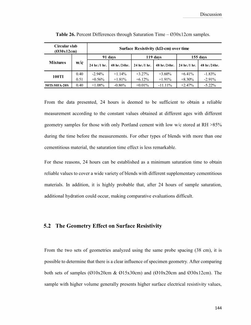
Discussion
144
Table 26. Percent Differences through Saturation Time – Ø30x12cm samples.
From the data presented, 24 hours is deemed to be sufficient to obtain a reliable
measurement according to the constant values obtained at different ages with different
geometry samples for those with only Portland cement with low w/c stored at RH >85%
during the time before the measurements. For other types of blends with more than one
cementitious material, the saturation time effect is less remarkable.
For these reasons, 24 hours can be established as a minimum saturation time to obtain
reliable values to cover a wide variety of blends with different supplementary cementitious
materials. In addition, it is highly probable that, after 24 hours of sample saturation,
additional hydration could occur, making comparative evaluations difficult.
5.2 The Geometry Effect on Surface Resistivity
From the two sets of geometries analyzed using the same probe spacing (38 cm), it is
possible to determine that there is a clear influence of specimen geometry. After comparing
both sets of samples (Ø10x20cm & Ø15x30cm) and (Ø10x20cm and Ø30x12cm). The
sample with higher volume generally presents higher surface electrical resistivity values,
0.40 -2.94% +1.14% +3.27% +3.60% +6.41% -1.83%
0.51 +0.56% +1.81% +6.12% +1.91% +8.30% -2.91%
50TI-30FA-20S 0.40 +1.08% -0.86% +0.01% -11.11% +2.47% -5.22%
100TI
Circular slab
(Ø30x12cm)Surface Resistivity (kΩ-cm) over time
Mixtures w/c91 days 119 days 155 days
24 hr./1 hr. 48 hr./24hr. 24 hr./1 hr. 48 hr./24hr. 24 hr./1 hr. 48 hr./24hr.
Discussion
145
even after the geometry correction factor was applied. However, it was also found that, if
the volume relation of the cylindrical samples is closer to 1.0 (i.e. Vol. Ø10x20cm/Vol.
Ø15x30cm is closer to 1.0 than Vol. Ø10x20cm/Vol. Ø30x12cm) the surface resistivity
difference is going to be minor if the storage condition and saturation degree were the same
before testing regardless of the sample’s age.
Based on data from Table 19 from Section 4.2.1, it can be seen in Figures 80 and 81 that
the relation between the circular slabs and the standard cylinders can be represented by a
linear trend. The “Line of Equality” represents the volume relation, values below the line
indicate that Ø10x20cm sample has higher resistivity value; above the line is the
Ø30x12cm sample has the higher value. In Figure 80, the trend lines can be seen for
mixture 50TI30FA20S stored in tap water (TW) and limewater (LW). Due to the
significantly lower resistivity values, the trendlines for the Portland mixtures can be seen
in detail in Figure 81.
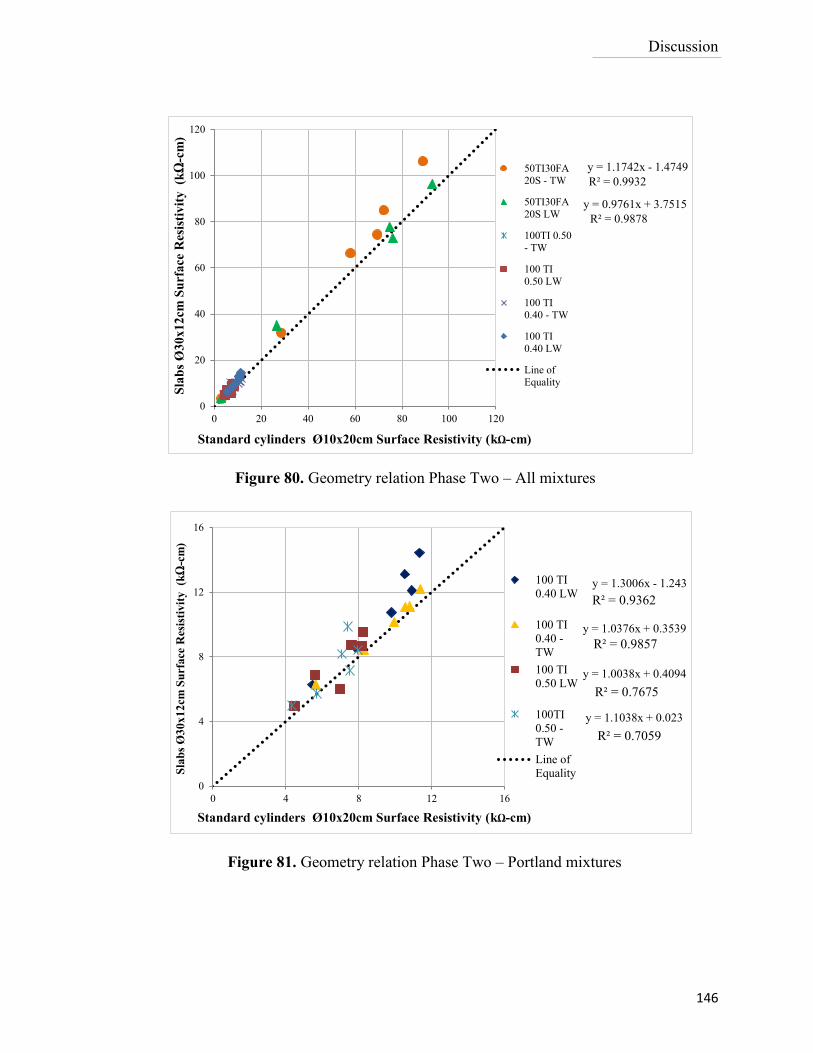
Discussion
146
Figure 81. Geometry relation Phase Two – Portland mixtures
Figure 80. Geometry relation Phase Two – All mixtures
y = 1.1742x - 1.4749
R² = 0.9932
y = 0.9761x + 3.7515
R² = 0.9878
0
20
40
60
80
100
120
0 20 40 60 80 100 120
Sla
bs
Ø3
0x1
2cm
Su
rfa
ce R
esis
tiv
ity
(k
Ω-c
m)
Standard cylinders Ø10x20cm Surface Resistivity (kΩ-cm)
50TI30FA
20S - TW
50TI30FA
20S LW
100TI 0.50
- TW
100 TI
0.50 LW
100 TI
0.40 - TW
100 TI
0.40 LW
Line of
Equality
y = 1.3006x - 1.243
R² = 0.9362
y = 1.0038x + 0.4094
R² = 0.9857
y = 1.0376x + 0.3539
R² = 0.7675
y = 1.1038x + 0.023
R² = 0.7059
0
4
8
12
16
0 4 8 12 16
Sla
bs
Ø3
0x
12
cm S
urf
ace
Res
isti
vit
y
(kΩ
-cm
)
Standard cylinders Ø10x20cm Surface Resistivity (kΩ-cm)
100 TI
0.40 LW
100 TI
0.40 -
TW
100 TI
0.50 LW
100TI
0.50 -
TW
Line of
Equality
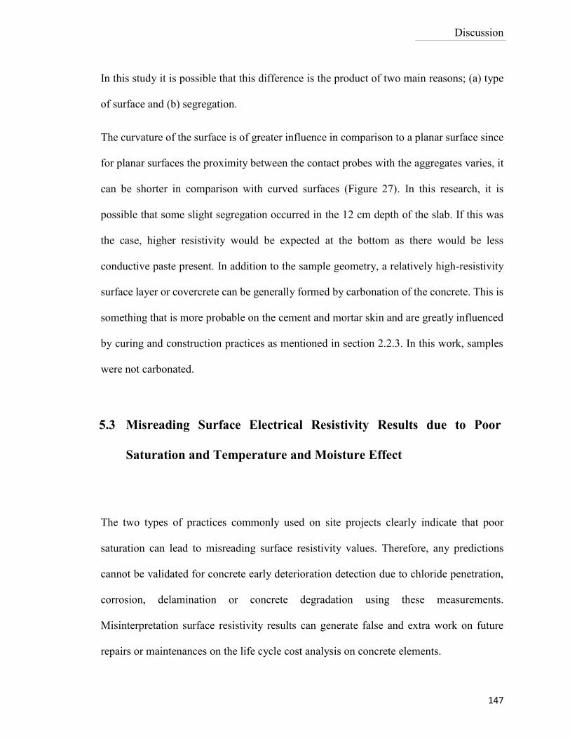
Discussion
147
In this study it is possible that this difference is the product of two main reasons; (a) type
of surface and (b) segregation.
The curvature of the surface is of greater influence in comparison to a planar surface since
for planar surfaces the proximity between the contact probes with the aggregates varies, it
can be shorter in comparison with curved surfaces (Figure 27). In this research, it is
possible that some slight segregation occurred in the 12 cm depth of the slab. If this was
the case, higher resistivity would be expected at the bottom as there would be less
conductive paste present. In addition to the sample geometry, a relatively high-resistivity
surface layer or covercrete can be generally formed by carbonation of the concrete. This is
something that is more probable on the cement and mortar skin and are greatly influenced
by curing and construction practices as mentioned in section 2.2.3. In this work, samples
were not carbonated.
5.3 Misreading Surface Electrical Resistivity Results due to Poor
Saturation and Temperature and Moisture Effect
The two types of practices commonly used on site projects clearly indicate that poor
saturation can lead to misreading surface resistivity values. Therefore, any predictions
cannot be validated for concrete early deterioration detection due to chloride penetration,
corrosion, delamination or concrete degradation using these measurements.
Misinterpretation surface resistivity results can generate false and extra work on future
repairs or maintenances on the life cycle cost analysis on concrete elements.
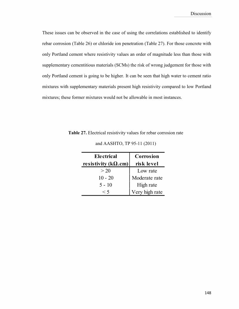
Discussion
148
These issues can be observed in the case of using the correlations established to identify
rebar corrosion (Table 26) or chloride ion penetration (Table 27). For those concrete with
only Portland cement where resistivity values an order of magnitude less than those with
supplementary cementitious materials (SCMs) the risk of wrong judgement for those with
only Portland cement is going to be higher. It can be seen that high water to cement ratio
mixtures with supplementary materials present high resistivity compared to low Portland
mixtures; these former mixtures would not be allowable in most instances.
> 20 Low rate
10 - 20 Moderate rate
5 - 10 High rate
< 5 Very high rate
Electrical
resistivity (kΩ.cm)
Corrosion
risk level
Table 27. Electrical resistivity values for rebar corrosion rate
and AASHTO, TP 95-11 (2011)
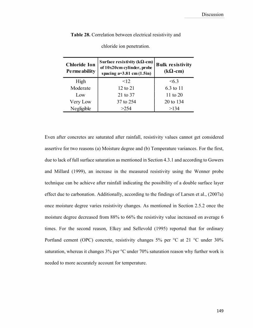
Discussion
149
Even after concretes are saturated after rainfall, resistivity values cannot get considered
assertive for two reasons (a) Moisture degree and (b) Temperature variances. For the first,
due to lack of full surface saturation as mentioned in Section 4.3.1 and according to Gowers
and Millard (1999), an increase in the measured resistivity using the Wenner probe
technique can be achieve after rainfall indicating the possibility of a double surface layer
effect due to carbonation. Additionally, according to the findings of Larsen et al., (2007a)
once moisture degree varies resistivity changes. As mentioned in Section 2.5.2 once the
moisture degree decreased from 88% to 66% the resistivity value increased on average 6
times. For the second reason, Elkey and Sellevold (1995) reported that for ordinary
Portland cement (OPC) concrete, resistivity changes 5% per °C at 21 °C under 30%
saturation, whereas it changes 3% per °C under 70% saturation reason why further work is
needed to more accurately account for temperature.
High <6.3
Moderate 6.3 to 11
Low 11 to 20
Very Low 20 to 134
Negligible >134
12 to 21
21 to 37
37 to 254
>254
Chloride Ion
Permeability
Bulk resistivity
(kΩ-cm)
Surface resistivity (kΩ-cm)
of 10x20cm cylinder, probe
spacing a=3.81 cm (1.5in)
<12
Table 28. Correlation between electrical resistivity and
chloride ion penetration.
150
6 Conclusions
1. It was found for standard cylinders Ø10x20cm and Ø30x12cm slabs, particularly
for those mixtures with only Portland cement with low w/c, that the minimum
saturation time duration to achieve a reliable measured resistivity value is 24 hours.
For other types of blends with different cementitious materials, 24 hours can be
considered sufficient as after this time additional hydration could occur, making
comparative evaluations difficult.
2. The use of supplementary cementitious materials, such as fly ash and granulated
blast-furnace slag are highly recommended. Their use generates a more complex
and refined pore network as it was confirmed during the test conducted in this
research. For these mixtures, resistivity increased significantly over time.
3. For those mixtures containing both fly ash and slag (50TI30FA20S and
50TI20FA30S) compared to mixtures with 100TI at similar water cement ratio
(w/c), the pore solution conductivity is on average 1.78 times less and 10 times
higher for electrical resistivity. The pore solution is only one factor in determination
of the surface resistivity.
Conclusions
151
4. The standardized laboratory method AASHTO TP 95 – 11 requires the storage of
samples in limewater (diluted solution of calcium hydroxide) with volume ratio less
or equal to 3:1 or 100% humidity, something that is difficult to achieve for on-site
testing. In this research it was found that the use of tap water is feasible for
saturation purposes. At early ages (7 and 28 days) there is not a clear major
influence between limewater and tap water. However, at or after 56 days, the use
of limewater leads to surface resistivity on average higher than that measured on
those submerged continuously in tap water. A correction factor may be necessary
at later ages. More work is needed to verify these findings.
5. The correction factor established by Spragg et al. (2013) helps to reduce the
differences between sample geometries, but the large volumes still yielded higher
surface resistivity. This can be due to the type of surface (curved or planar), the
presence of segregation as well as surface roughness that can generate variations.
6. The correlations to normalize temperature based on standard cylinder geometry
were not able to account for differences between laboratory and on-site resistivity
measurements. More work is needed in this area.
7. Significant differences were obtained between the two tested saturation techniques
and full laboratory saturation. Poor surface saturation as presented by using
pressurized water and static ponding can lead to misinterpretation of resistivity of
over 30% (average) even after rainfall lead to unreliable resistivity values.
Conclusions
152
8. The correlations established to identify rebar corrosion or chloride ion penetration
as there is not a clear difference between the influence of water to cement ratio
(w/c) or the use of supplementary cementitious materials (SCMs).
153
7 Recommendations
1. Further monitoring the cast samples used in Phase 2 can be completed to continue
evaluate the resistivity performance over time, checking the increasing rate on the
different mixtures. Also, it is possible to continue verifying if the differences in
geometry and storage solutions remain or significant changes occur.
2. Although in this research all the measurements made in the laboratory were made
under the same conditions, samples stored at RH>85% before testing and during
testing time, samples were immersed into limewater or tap water solution at same
temperature. Further effort can be made to compare the results obtained estimating
the changes under different solution types and temperatures as well as stored under
different moisture conditions before testing.
3. Furthermore, it is suggested to continue simulating the onsite saturation by water
pressure or static ponding saturation and to further understand how much time is
required for water to penetrate through concrete surface. Relative humidity sensors
can be installed inside the circular slabs to support the findings achieved in this
study. On each slab, a minimum number of 4 sensors can be installed that penetrate
10 cm inside from the circular slab edge. Each sensor can be spaced 1 cm from each
other in the vertical axis, starting at 1 cm below the top surface.
154
4. In order to address the differences in surface resistivity due to geometry, the effect
of type of surfaces (curved and planar) and correlations to normalize temperature,
more different sets of samples can be tested. Ideally, increasing the number and
variety of samples, including non-cylindrical geometries with different volumes
can be cast using different mixtures and aggregate sizes. Then a comparison can be
made with standard geometry samples (i.e. Ø10x20cm). Also verification can be
made between the results achieved between the simulations developed by Morris
et al. (1996). On the other hand, a simple cut of (1 to 2 cm) from the edge of standard
cylinders (Ø10x20 and Ø15x30cm) through all vertical length of the cylinder can
be done to evaluate and monitor differences between curved and plane surfaces and
then establish a correction factor base on this findings.
5. Moreover, Gowers and Millard (1999) state that the sample thickness should be at
least 4 times the probe spacing. Although the 10 cm diameter samples do not meet
this criterion with 38 mm spacing, this combination is by far the most commonly
used in practice. A review can be done in future to update this condition and
establish possible influences.
6. To address the issue with the correlations to normalize the temperature effect, the
samples can be tested in conjunction with the temperature and humidity sensors so
it could be possible to update the correlations established by Liu et al., (2014) based
only on standard cylinders (10x20cm). Additionally these samples can be stored
155
under different moisture degrees before testing and monitored over time under
different temperatures.
156
References
1. Andrade, C., and Alonso, C., (1996) “Corrosion Rate Monitoring in the Laboratory
and On-site”, Construction & Building Materials, V.10. pp. 315 – 328.
2. ASP Construction (2003) “Health and Safety on Construction Sites Course”
Student’s Manual, 5th Edition, Revised Edition 2003.
3. AASHTO, TP 95-11 (2011) “Standard Method of Test for Surface Resistivity
Indication of Concrete’s Ability to Resist Chloride Ion Penetration.” AASHTO
Provisional Standards, 2011 Edition.
4. AASHTO T 277-05 (2007) “Standard Method of Test for Electrical Indication of
Concrete's Ability to Resist Chloride Ion Penetration” AASHTO, 2007 Edition.
5. ASTM C1611 / C1611M – 14 (2014) “Standard Test Method for Slump Flow of
Self-Consolidating Concrete”. American Society of Testing and Materials
(ASTM). Book of Standards Volume: 04.02
6. ASTM C39 / C39M - 14a (2014) “Standard Test Method for Compressive Strength
of Cylindrical Concrete Specimens”. American Society of Testing and Materials
(ASTM). Book of Standards Volume: 04.02
157
7. ASTM Test C 666, (2008) “Mechanical Properties and Freezing and Thawing
Resistance of Non-Air-Entrained, Air-Entrained, and Air-Entrained
Superplasticized Concrete”. American Society of Testing and Materials (ASTM).
8. ASTM C1202-12, (2012) “Standard Test Method for Electrical Indication of
Concrete’s Ability to Resist Chloride Ion Penetration”, American Society of
Testing and Materials (ASTM). EDT 2012.
9. Baker, R.F.M., (1985) “Illustration of Permeability and Porosity. Diffusion within
and into Concrete”, Paper presented at 13th Annual Convention of the Institute of
Concrete Technology, University of Loughborough. Slough Institute of Concrete
Technology. pp.21.
10. Barneyback, S., and S. Diamond (1981) “Expression and Analysis of Pore Fluids
from Hardened Cement Pastes and Mortars”. Cement and Concrete Research,
Vol.11, No.2, pp. 279-285.
11. Bassuoni, M. T., Nehdi M. L., and Greenough T. R. (2006) “Enhancing the
Reliability of Evaluating Chloride Ingress in Concrete Using the ASTM C1202
Rapid Chloride Penetrability Test”, Journal of ASTM International, Vol. 3, No. 3,
pp. 1-13.
158
12. Belviso, C.; Pascucci, S.; Cavalcante, F.; Palombo, F.; Pignatti, F.; Simoniello, T;
and Fiore, Saverio (2011) “Multi-Technique Application for Waste Material
Detection and Soil Remediation Strategies: The Red Mud Dust and Fly Ash Case
Studies, Soil Contamination”, ISBN: 978-953-307-647-8, InTech, DOI:
10.5772/24886. <http://www.intechopen.com/books/soil-contamination/multi-
technique-application-for-waste-material-detection-and-soil-remediation-
strategies-the-red-mud>, accessed 16 November 2014.
13. Bentz, D. A. (2007) “Virtual Rapid Chloride Permeability Test”. Cement and
Concrete Composites, Vol. 29, No.10, pp. 723 – 731.
14. Bockris, J.O. and Reddy, A.K (2002) “Modern Electrochemestry 1: Ionics secod
edition, Plenum Press, New York, 2002. pp.769.
15. Bryant, W. J., Weyers, E. R., M. de la Garza, J. (2009) “In – Place Resistivity of
Bridge Deck Concrete Mixtures,” ACI Materials Journal, March – April, Vol. 106,
no. 2, pp. 114 -122.
16. Castro, J., Spragg, R., and Weiss, J. (2012) “Water Absorption and Electrical
Conductivity for Internally Cured Mortars with a W/C between 0.30 and 0.45”
.Journal of Materials in Civil Engineering, Vol. 24, No. 2. pp. 223–231.
159
17. Chini A. R., Muszynski L. C., and Hicks J., (2003) “Determination of Acceptance
Permeability Characteristics for Performance-Related Specifications for Portland
Cement Concrete”, Final report submitted to FDOT (MASc. Thesis), University
of Florida, Department of Civil Engineering.
18. Chun-Tao Chen, Jiang-Jhy Chang, Wei-chung Yeih. (2014) “The effects of
specimen parameters on the resistivity of concrete” Journal of Construction and
Building Materials 71- Elsevier Ltd (September - 2014). Vol, 71, pp. 35-43.
19. DeSouza, Savio John, (1996) “Test Methods for the Evaluation of the Durability of
Covercrete” M.A.Sc. Thesis University of Toronto, Department of Civil
Engineering. pp. 88.
20. Di Bella, C., C. Villani, N. Phares, R. Hausheer, and J.Weiss (2012) “Chloride
Transport and Service Life in Internally Cured Concrete”. Presented at the
Structures Congress 2012, Chicago.
21. Dullien, F. (1992) “Porous Media: Fluid Transport and Pore Structure”. Academic
Press, San Diego.
22. Elkey, W. and Sellevold, E.J. (1995) “Electrical Resistivity of Concrete Norwegian
Public Roads Administration Publication, 1995. 33 pp.
160
23. Flower, DJM; Sanjayan JG. (2007) “Green House Gas Emissions due to Concrete
Manufacture”. Department of Civil Engineering, Monash University, Clayton, VIC
3800, Australia. Int J LCA 12 (5). pp. 282–288.
24. Gowers, K.R. and Millard, S.G, (1999) “Measurement of Concrete Resistivity for
Assessment of Corrosion Severity of Steel Using Wenner Technique” ACI
Materials Journal, Technical paper, September - October 1999, Vol. 96, No. 5, pp.
536-541.
25. Heubeck, Christoph (2004) “Packing, Porosity, and Permeability lecture for the
Earth History”. Institut für Geologische Wissenschaften Freie Universität Berlin.
pp15.
26. Hooton, R. Doug. (1989) “What is needed in a Permeability Test for Evaluation of
Concrete Quality”, Materials Research Society 1989, Vol.137, pp.141-149.
27. Hornbostel, K., Larsen, C.K., and Geiker, M.R. (2013) “Relationship between
Concrete Resistivity and Corrosion Rate: A literature Review”, Cement and
Concrete Composites, V.39. pp. 60-72.
28. Kessler, R.J.; Powers, R.G.; Paredes, M.A.; (2005) “Resistivity Measurements of
Water Saturated Concrete as an Indicator of Permeability,” Corrosion 2005, April
3-7 2005. Paper 05621, pp. 1-10.
161
29. Kessler, R.J.; Powers, R.G.; Vivas, E.; Paredes, M.A.; and Virmani, P., (2008)
“Surface Resistivity as an Indicator of Concrete Chloride Penetration Resistance,”
Concrete Bridge Conference, May 4-7, St. Louis, pp. 1 -17.
30. Kosmatka, Steven H.; Kerkhoff, Beatrix; Panarese, William C.; MacLeod, Norman
F.; and McGrath Richard J., (2002) “Design and Control of Concrete Mixtures”,
EB101, 7th Editio, Cement Association of Canada, Otawa, Ontario. pp, 368.
31. Kreijger, P.C; (1984) “The Skin of Concrete – Composition and Properties”,
Matériux et Constructions. Vol.17, No. 100, pp. 275-283.
32. Larsen, C.K; Sellevold, E.J; Askeland, F; Østvik, J.M and Vennesland, Ø, (2007a)
“Electrical Resistivity of Concrete. Part II: Influence of Moisture Content and
Temperature”. Norwegian Public Roads Administration, Technology Department
Report No. 2482, pp. 16-24.
33. Larsen, C.K; Sellevold, E.J; Østvik, J-M.; and Vennesland Ø, (2007b) “Electrical
Resistivity of Concrete. Part III: Long Term Field Measurements on Concrete
Elements in the Tidal Zone”. Norwegian Public Roads Administration, Technology
Department Report No. 2482, pp. 25-38.
162
34. Lataste, J. F; Breysse, D and Frappa, M, (2003) “ Electrical Resistivity
Measurement applied to Cracking Assessment on Reinforced concrete Structures
in Civil Engineering” NDT & E International, Vol. 36, No. 06, pp. 383-394.
35. Liu, Yanbo and Presuel-Moreno , (2014) “ Normalization of Temperature Effect
on Concrete Resistivity by Method Using Arrhenius Law” American Concrete
Institute (ACI) Materials Journal. Title No. 11-M39. ACI Materials Journal/July-
August 2014, pp. 433-442.
36. Lippiatt, B., and S. Ahmad, (2014) “Measuring the Life-Cycle Environmental and
Economic Performance of Concrete: The BEES Approach”. International
Workshop on Sustainable Development and Concrete Technology, Beijing.
37. Lopez W. and Gonzalez J. A. (1993), “Influence of the Degree of Pore
Saturation on the Resistivity of Concrete and the Corrosion Rate of Steel
Reinforcement”. Cement and Concrete Research, Vol. 23, No. 2, pp. 368-376.
38. McCarter W. J., Starrs G., Kandasami S., Jones R., and Chrisp T.M., (2009)
“ Electrode Configuration for Resistivity Measurements on Concrete”, ACI
Materials Journal, Vol.106, No. 3, pp. 258-264.
39. McCarter, W. J. (1996) “Monitoring the Influence of Water and Ionic Ingress on
Cover-Zone Concrete Subjected to Repeated Absorption”, Cement, Concrete and
Aggregates, Vol. 18, No. 1, pp.55-63.
163
40. Millard S.G., Harrison J.A., Edwards A.J. (1989) “Measurement of the electrical
resistivity of reinforced concrete structures for the assessment of corrosion risk”.
Brit J NDT 1989; 31(11). pp. 617–621.
41. Millard S. G. and Gowers K. R., (1991) “The Influence of Surface Layers upon the
Measurement of Concrete Resistivity, Durability of Concrete”, Second
International Conference, ACI SP-126, Montreal, Canada, pp. 1197-1220.
42. Morris W., Moreno E. I., and Sagues A. A., (1996) “Practical Evaluation of
Resistivity of Concrete in Test Cylinders Using A Wenner Array Probe,
Cement and Concrete Research”, Vol. 26, No. 12, pp. 1779-1787.
43. Monfore, G. E. (1968), “ The Electrical Resistivity of Concrete, Journal of the
PCA Research Development Laboratories”, Vol. 10, No. 2, pp. 35-48.
44. Montgomery, T., Jiang L., Sherman M. R., and Schlagel D. (2013) “Tackling
Freezing-and-Thawing Deterioration of Historic Stadia. A 5-year rehabilitation of
the Notre Dame Old Bowl Football Stadium”. Concrete International Magazine.
Vol, 35, NO. 4 pp.38 – 44.
45. Neville, A.M. and Brooks, J.J. (1987), Concrete Technology, Longman, Harlow.
164
46. Nokken, M. R. and Hooton, R. D., (2006) “Electrical Conductivity as a
Prequalification and Quality Control,” Concrete International, Vol. 28, No. 10,
2006, pp. 61-66.
47. Polder, R.B. and Larbi, J.A. (1995) “Investigation of Concrete Exposed to North
Sea Water Submersion for 16 Years”. HERON 40, pp. 31-56.
48. Polder, R.B, Andrade, C., Elsener, C., Vennesland, Ø. Gulikers, J., Weidert, R.,
Raupach, M. (2000) “Test methods for onsite measurement of resistivity of
concrete”. RILEM TC-154 -EMC: Electrochemical Techniques for Measuring
Metallic Corrosion. Materials and Structures/Mat6riaux et Constructions, Vol. 33,
December 2000, pp. 603-611.
49. Polder, R.B. (2001) "Test Methods For On Site Measurement of Resistivity of
Concrete—A RILEM TC-154 Technical Recommendation". Construction and
Building Materials Vol. 15. No. 2, pp. 125-131.
50. Polder, R.B. and de Rooij, M.R. (2005) “Durability of Marine Concrete Structures
– Field Investigations and Modelling”. HERON 50, pp. 133-143
51. Powers, T.C., (1960). “Chemistry of Cement Proceedings”, 4th International
Symposium, Washington DC, National Bureau of Standards, Monograph 43, US
Deparment of Commerce, Washington DC Paper V-1 (192), pp. 577-613.
165
52. Powers, T.C., Copeland, L.E., Mann, H.M., (1959) “Capillary continuity or
discontinuity in cement pastes”. Journal of the PCA Research and Development
Laboratories. 1(2): p. 38-48.
53. Presuel-Moreno, Francisco; Suares, Andres; Liu, Yanbo, (2010) “Characterization
of New and Old Concrete Structures Using Surface Resistivity Measurements,”
Final Report. Florida Department of Transportation (Contract No. BD546, RPWO
#08).
54. Presuel-Moreno, Francisco; Liu, Yanbo, (2012) “Temperature Effect on Electrical
Resistivity Measurements on Mature Saturated Concrete” Nace International
Conference & Expo Corrosion 2012, (NACE-2012-1732) pp. 5678-5696.
55. Rađenović, A.; Malina, J.; and Sofilić T. (2013) “Characterization of Ladle Furnace
Slag from Carbon Steel Production as a Potential Adsorbent”, Advances in
Materials Science and Engineering, Volume 2013 (2013), Article ID 198240. pp 6.
56. Proceq SA manual (2013) “Resipod Resistivity Mete”. Code 810 381 01E V.06
(2013) Proceq SA, Switzerland, <http://www.proceq.com/non-destructive-test-
equipment/concrete-testing/moisture-corrosion-analysis/resipod.html >, accessed
21 January 2015.
166
57. Rupnow, Tyson D; and Icenogle, Patrick. (2011) “Evaluation of Surface Resistivity
Measurements as an Alternative to the Rapid Chloride Permeability Test for
Quality Assurance and Acceptance,” Final Report (July 2011). Louisiana
Department of Transportation and Development.
58. Savas B. Z., (1999), “Effect of Microstructure on Durability of Concrete” PhD
Thesis, North Carolina State University, Department of Civil Engineering, Raleigh
NC.
59. Slagment, (2010), AfriSam Products and Services, <
http://www.afrisam.co.za/products-services/cement/slagment/ >. Accessed: 18
October 2014.
60. Shahroodi, Ahmad. (2010) “Development of Test Methods for Assessment of
Concrete Durability for Use in Performance-Based Specifications” M.A.Sc.
University of Toronto, Department of Civil Engineering, pp. 219.
61. Shi C., (2004) “Effect of Mixing Proportions of Concrete onits Electrical
Conductivity and the Rapid Chloride Permeability Test (ASTM C1202 or
ASSHTO T277) Results”, Cement and Concrete Research, Vol. 34, No. 3, 2004,
pp. 537-545.
167
62. Spragg, R. (2013) “The Rapid Assessment of Transport Properties of Cementitious
Materials Using Electrical Methods”.M.S.C.E. Purdue University, West Lafayette,
Indiana.
63. Spragg, R., Bu, Y., Snyder, K., Bentz, D., Weiss, J. (2013a) “Electrical Testing of
Cement-Based Materials: Role of Testing Techniques, Sample Conditioning, and
Accelerated Curing” Final Report. Joint Transportation Research Program, Indiana
Department of Transportation and Purdue University. Report Number:
FHWA/IN/JRTP-2013/28. DOI: 10.5703/1288284315230. pp. 1- 19.
64. Spragg, R., Villani, C., Snyder, K., Bentz, D., Bullard, J., and Weiss, J. (2013b)
“Electrical Resistivity Measurements in Cementitious systems: Observations of
Factors that influence the Measurements”. Transportation Research Record:
Journal of the Transportation Research Board, Vol. 2342, Concrete Materials. pp.
90 – 98.
65. Snyder, K., Feng, X., Keen, B., and Mason, T. (2003) “Estimating the Electrical
Conductivity of Cement Paste Pore Solution from OH, K, and Na Concentrations”.
Cement and Concrete Research, Vol. 33, No. 6, pp. 793 – 798.
66. Swamy, R. N., (1996) “High Performance Durability through Design” International
Workshop on High Performance Concrete, SP – 159, P. Zia, ed., American
Concrete Institute, Farmington Hills, MI. pp.209 – 230.
168
67. Stanish K., Hooton R. D., and Thomas M. D. A.(1997), “Testing the Chloride
Penetration Resistance of Concrete: A Literature Review”, Department of Civil
Engineering University of Toronto, Toronto, Ontario, Canada, FHWA Contract
DTFH61-97-R 00022.
68. Strategic Highway Research Program (SHRP2), Condition Assessment,
Technologies –Electrical Resistivity – NDToolbox, <
http://www.ndtoolbox.org/content/bridge/er-description >, accessed 21 January
2015.
69. Taylor P., Tennis P., Obla K., Ram P., Van Dam T., and Dylla H. (2013),
“Durability of Concrete”, Second Edition, Transportation Research Circular E-
C171. September 2013. Transportation Research Board Durability of the National
Academies. pp. 1-78.
70. Wei, X., and Li, Z., (2006) “Early Hydration Process of Portland Cement Paste by
Electrical Measurement”. Journal of Materials in Civil Engineering, ASCE, V.18,
No. 1. pp. 99-105.
71. Wenner, F. (1916) “A Method of Measuring Earth Resistivity”. Bulletin of the
National Bureau of Standards, Vol.12, pp.469-478.