Appendix A-2

Journal Paper: Submitted to ASCE Journal of Engineering Mechanics, June 2004 Accepted September 2004

Influence of Implicit Integration Scheme on Prediction of

Shear Band Formation

Randall J. Hickman1 and Marte Gutierrez, M.ASCE2

1Graduate Student, Dept. of Civil Engineering, Virginia Polytechnic Institute & State University, Blacksburg, VA 24061

2Assoc. Professor, Dept. of Civil Engineering, Virginia Polytechnic Institute & State

University, Blacksburg, VA 24061

Corresponding address: Marte Gutierrez, PhD Civil & Environmental Engineering Virginia Polytechnic Institute & State University 200 Patton Hall, Blacksburg, VA 24061 Tel: 540-231-6357, Fax: 540-231-7532 E-mail: magutier@vt.edu

374

Abstract: Implicit integration schemes for elastoplastic constitutive equations have been

developed in recent years as an alternative to explicit schemes. The consistent tangent

constitutive matrix Dcon that results from implicit schemes makes the global stiffness matrix

consistent with the implicit integration procedure, and differs from the traditional continuum

tangent constitutive matrix Dep that results from explicit schemes. Onset of strain localization

and shear banding has been traditionally predicted using the continuum tangent constitutive

matrix. It is shown that different criteria for onset of shear-band formation are obtained

depending on whether Dcon or Dep is used. It is shown that shear band prediction using Dcon is

step-size dependent, and that the use of Dcon influences the predicted onset of strain localization

in frictional materials. An analytical equation for prediction of the onset of shear-band

formation using Dcon for the Mohr-Coulomb model is developed, and a numerical example is

presented.

CE database subject headings: Bifurcations; Constitutive models; Elastoplasticity;

Localization

375

Introduction

The use of implicit integration schemes to solve for elastoplastic response of geomaterials has

increased in use in recent years (Runesson 1987; Borja and Lee 1990; Jeremic and Sture 1997;

Manzari and Nour 1997). The main feature of implicit algorithms is the use of the final stress

point in the constitutive response in calculating all the relevant derivatives and internal

variables required in the constitutive relations (Simo and Taylor 1985; Jeremic and Sture 1997).

Since this point is not known in advance, a set of Newton iterations is used to advance the

solution toward the final point for each load increment. In comparison, explicit integration

schemes use the initial stress point to determine the derivatives and internal variables required

to form the constitutive relations. Since a solution is assumed to exist, implicit methods

generally guarantee that a converged solution will be obtained on the constitutive level, even

for highly nonlinear models (Ortiz and Popov 1985). The resulting discretized constitutive

relation obtained using implicit schemes is called the consistent tangent operator or the

consistent tangent constitutive matrix Dcon, and differs considerably from the continuum

tangent constitutive matrix Dep obtained using explicit schemes. A compact expression of Dcon

was obtained by Jeremic and Sture (1997).

In finite element analysis, the use of consistent tangent matrix Dcon and implicit integration

schemes is fast becoming the preferred method in implementing many types of elastoplastic

constitutive models for any local integration scheme (Miehe 1996; Alfano and Rosati 1998;

Perez-Fouget et al. 2001; Jirasek and Patzak 2002). The main motivation is that the use of Dcon

to form the global stiffness matrix for a finite element assemblage preserves the quadratic

convergence of the iterative global convergence method, and thus achieves faster convergence

in finite element calculations than the use of Dep (Simo and Taylor 1985). Dep evaluates the

376

gradients to the yield surface and to the plastic potential surface at the same stress point,

namely the initial stress point. In comparison, Dcon is formulated to be consistent with the

integration method, and so evaluates the gradients to the yield surface and to the plastic

potential surface at different stress points. Therefore, Dcon is generally non-symmetric even

when applied to models with associated flow rules. In contrast, Dep is only non-symmetric for

non-associated flow.

Non-symmetry of the constitutive matrix D causes the acoustic tensor B (defined below) to

become non-positive definite and produces negative eigenvalues for certain wave propagation

directions. In bifurcation theory, such negative eigenvalues imply strain localization and

instability, following Mandel’s (1964) stability criterion. It is to be noted that Mandel’s

criterion is a necessary and sufficient criterion to detect the onset of instability in material. As a

result of non-symmetry in the constitutive and/or global stiffness matrices, localized

deformations may occur during finite element calculations. Localization of deformation is

extensively observed in many geomaterials subjected to large deformations. The most common

type of localized deformation in geomaterials is the shear band, although other types of

localized deformation such as the compaction band and dilation band are also observed and

may be predicted (Olsson 1999; Issen and Rudnicki 2000; DuBernard et al. 2002; Issen and

Challa 2003). The localization of deformation was first treated as a bifurcation problem by

Rudnicki and Rice (1975), in which a material undergoing homogenous deformation reaches a

bifurcation point, experiences material instability, and deformation becomes non-homogenous.

Extensive experimental studies have been performed on frictional-cohesive geomaterials by

Arthur et al. (1977), Ord et al. (1991), Besuelle (2001), and Lade (2002), among others, and

have shown that shear bands can form before the peak strength of material is mobilized.

377

Numerous analytical and numerical studies have been performed to simulate various

phenomena observed during strain localization: these include efforts to promote strain

localization by introducing vertex-like areas to the yield surface (Rudnicki and Rice 1975;

Bardet 1991), and efforts to simulate strain localization in finite element structures using

gradient plasticity (Bazant and Pijaudier-Cabot 1988; deBorst and Muhlhaus 1992) and

Cosserat continua (deBorst 1991).

A review of the different studies that have been performed so far reveals that, as yet,

implicit integration schemes and their effects on prediction of shear band formation have not

been investigated. This is despite the fact that implicit schemes are now gaining wide

acceptance and use in constitutive and finite element modeling. Three properties of Dcon may

affect the prediction of shear band formation. These properties include: 1) non-symmetry for

associated flow, 2) reduced stiffness, and 3) step-size dependence. The effects of using Dcon

instead of Dep to predict the onset of strain localization are investigated in this paper.

The objective of this paper is to show the effects of using implicit integration schemes in

predicting the onset of strain localization in frictional-cohesive geomaterials. This article is

concerned only with the conditions for instability in a geomaterial and the ability to predict the

onset of instability and shear band formation using constitutive equations. Simulation of

post-localization or post-bifurcation material response is not addressed.

General Equations

Background information related to this work is presented in this section. These include a

description of implicit integration schemes and the elastoplastic constitutive matrix, and a

description of bifurcation theory and its use to predict the onset of strain localization using the

elastoplastic constitutive matrix and the acoustic tensor.

378

Implicit Integration Schemes and the Elastoplastic Constitutive Matrix

Constitutive relations for most elastoplastic models are given by following set of equations:

(1) pij

eijij ddd ε+ε=ε

(2) ekl

eijklij dDd ε=σ

ij

pij

gdσ∂∂

λ=ε (3)

αα λ= hdq (4)

where , , and are the increments of the total, elastic, and plastic strain tensors; dijdε eijdε p

ijdε ijσ is

the increment of the Cauchy stress tensor; is the elastic constitutive tensor; is the plastic

multiplier;

eijklD λ

ijσg ∂∂ is the gradient to the plastic potential surface; is the set of plastic

hardening variables; and is the plastic hardening rule. Eqs. (1) to (4) represent the properties

of strain additivity, incremental elasticity, plastic flow rule, and plastic hardening rule,

respectively.

αq

αh

Eqs. (1) to (3) may be combined into a single equation to solve for the stress increment

for a given strain increment : ijdσ ijdε

σ∂∂

λ−ε=σij

kleijklij

gdDd (5)

Implementation of the constitutive model requires the numerical integration of Eqs. (1) to (4).

For rate-independent elastoplasticity, the values of f and λ are restricted by the Kuhn-Tucker

loading-unloading criterion:

( ) 0, =σ αqf ij (6)

0≥λ (7)

379

0=λf (8)

Eqs. (6) to (8) must be satisfied simultaneously for all loading conditions. Eq. (6) specifies

that the yield function must be non-positive for any set of stresses and hardening variables. For

elastoplastic loading, the stress point must lie on the yield surface at all stages of loading,

which generally requires that plastic strain occurs and λ > 0. The goal of a numerical

calculation for an elastoplastic loading step is to find the correct value of λ such that the final

stress point is consistent with the final yield surface (f = 0). Using Eqs. (4) and (5) to satisfy Eq.

(6):

0,

),(),(

0,0,

0,0,,,

=

λ+

σ∂∂

λ−ε+σ=

+σ+σ=σ

αα

ααα

hqgdDf

dqqdfqf

klkl

eijklij

ijijffij

(9)

For linear elastic models, the plastic flow direction is the only quantity in Eq. (9) that

depends on the loading increment and continuously evolves during loading. An additional

complication arises from nonlinear elasticity, where the elastic moduli also evolve during a

finite loading increment. Borja (1991) showed how to use secant elastic moduli with an implicit

integration scheme for such models. Implicit numerical integration schemes for elastoplasticity

satisfy Eq. (9) by using the plastic flow direction at the final stress point σij,f:

fij

ijfij

gg

,, σ

σ∂∂

=σ∂∂ (10)

Implicit integration schemes continually update the trial value of λ and the trial plastic

flow direction during the iterative solution process. As described by Jeremic and Sture (1997),

an approximate solution for the final plastic flow direction is attained readily as a function of

the derivatives of the plastic flow direction by using the first two terms of the Taylor series

380

expansion of Eq. (10), evaluated at the initial stress point σij,0:

α

σασσσ

∂σ∂∂

+σ

σ∂σ∂∂

+σ∂∂

≈σ∂∂

=σ∂∂ dq

qgdgggg

ijijijfijij

klklijijijfij

0,0,0,,

22

,

(11)

For finite element calculations, it is necessary to form a global stiffness matrix to calculate

displacements for the next loading step or global iteration. The global stiffness matrix is formed

using an elastoplastic constitutive matrix, which is either the continuum tangent constitutive

matrix Dep or the consistent tangent constitutive matrix Dcon. Dcon has been shown to promote

faster global convergence, as discussed earlier. These two constitutive matrices and their

differences in final form are discussed below.

Both Dep and Dcon are formed by combining Eq. (5) and Prager’s consistency condition:

α

α∂∂

+σσ∂∂

= dqqfdfdf ij

ij

(12)

Ultimately, both Dep and Dcon are formed using the difference between the elastic and plastic

tangent matrices:

HH

DfgDD

hqfgDf

DfgDDDDD

p

epqkl

pqmn

eijmn

eijkl

tu

erstu

rs

epqkl

pqmn

eijmn

eijkl

pijkl

eijkl

epijkl +

σ∂∂

σ∂∂

−=

∂∂

−σ∂∂

σ∂∂

σ∂∂

σ∂∂

−=−=

αα

0,

0,

0, (13a)

HH

RfmRR

hqfmRf

RfmRRRRD

p

epqkl

pqmn

eijmn

eijkl

tu

erstu

rs

epqkl

pqmn

eijmn

eijkl

pijkl

eijkl

conijkl +

∂∂

∂∂

−=

∂∂

−∂∂

∂∂

∂∂

∂∂

−=−=σσ

σσ

σσ

αα

(13b)

where ijm σ∂∂ is a modified plastic flow direction that incorporates the projected change in

hardening parameter, Hp is the perfectly plastic modulus, H is the plastic hardening modulus,

and is a modified stiffness tensor that Jeremic and Sture (1997) call the “reduced stiffness eijklR

381

tensor”. The following expressions for Hp are obtained for Dep and Dcon:

0,tu

erstu

rsp

gDfHσσ ∂∂

∂∂

= for Dep and tu

erstu

rsp

mRfHσσ ∂∂

∂∂

= for Dcon (14)

Both Dep and Dcon can be expressed in a single general form:

{ }HH

EfQEE

hqfQEf

EfQEEDD

p

epqkl

pqmn

eijmn

eijkl

tuerstu

rs

epqkl

pqmn

eijmn

eijkl

conijkl

epijkl +

σ∂∂

−=

∂∂

−σ∂∂

σ∂∂

−=

αα

, (15)

In Eq. (15), is a general expression for the elastic constitutive matrix and is a general

expression for the plastic flow direction. The final forms of D

eijklE ijQ

ep and Dcon are not the same due

to the differences between and , as shown by Jeremic and Sture (1997) and as

summarized in Table 1.

eijklE ijQ

Several differences between Dep and Dcon may be noted. First, the terms used to form Dep

are constant at a given stress point, while the terms used to form Dcon are functions of the

magnitude of λ from the previous loading step. Since the magnitude of λ depends on the

magnitude of the loading step, Dcon is step-size-dependent, while Dep is step-size-independent.

Jeremic and Sture (1997) show that Dcon converges to Dep as λ→0, or for an infinitesimally

small elastoplastic loading step. Second, the terms mnmn gQ σ∂∂= and pqf σ∂∂ in Eq. (15) are

equal for associated flow, so and Depklij

epijkl DD = ep is symmetric for associated flow. In contrast,

the terms ( )α∂+σ∂∂= qgQ mnmn σ∂∂λ g mn2 and pqf σ∂∂ in Eq. (15) are not equal for

associated flow, so and Depklij

epijkl DD ≠ con is generally non-symmetric even for associated flow. A

third difference between Dep and Dcon is that the material stiffness is reduced when Dcon is used,

as will be demonstrated later.

382

Since Dcon aims to satisfy the constitutive response at the final stress point, its elements

may be viewed as local consistent tangent moduli between the initial and final stress point. In

contrast, Dep may be viewed as a tangential matrix since its components are based on the

derivatives at the current stress point. This difference between Dep and Dcon is shown

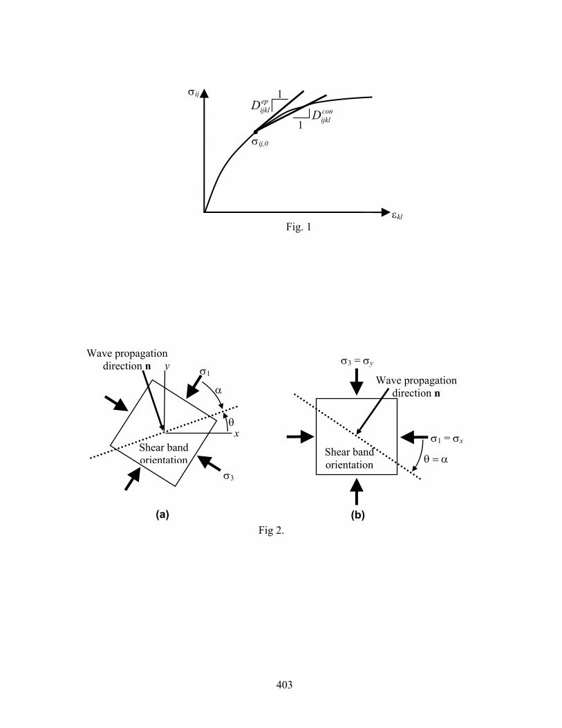
schematically in Fig. 1.

Bifurcation and Shear Band Formation

Bifurcation theory is concerned with the prediction of how instability leads to localized

deformations in elastoplastic materials. Strain localization manifests itself in cohesive-frictional

materials as a narrow zone in which the deformation rate exceeds that in the uniformly

deformed material. Since the yielding mechanism for these materials is shearing, the zone of

strain localization is called a shear band.

Prediction of strain localization is based on Mandel’s (1964) stability criterion which states

that a material is stable only when it is able to propagate small perturbations in the form of

waves. Instability and strain localization occur when a small perturbation in the form of a wave

cannot be propagated across a material in a given direction ni (i = 1,2,3). This condition appears

when the acoustic tensor B has a zero or negative determinant, becomes non-positive definite,

and produces negative eigenvalues. This condition may be stated for the case in which

co-rotational terms are neglected as:

0≤= lijkljik nDnB (16)

Bik is a function of the constitutive matrix D and of the direction of wave propagation n. The

shear band orientation is normal to n, as shown in Fig. 2.

For the two-dimensional, plane strain condition (i,j,k,l = 1,2), D may be expressed as a 3x3

matrix by deleting from the three-dimensional constitutive matrix the components which

383

correspond to out-of-plane straining:

1111 1122 1112

2211 2222 2212

1211 1222 1212

ijkl

D D DD D D D

D D D

=

(17)

In two dimensions, the unit vector n may be expressed in terms of the angle θ between the

shear band and the coordinate axes (i.e., between the normal to n and the x-axis):

1

2

sincosi

nn

nθ

= = θ (18)

The determinant B may then be expressed in terms of Dijkl and θ as:

( )( ) ( )( )( )( )

( )( )( )22121122221112222222121122221112

3

221112121212112222111122

22121211122211122222111122

221111121211112222121111122211113

22121222222212124

12111112121211114

cossin

cossin

cossin

cossin

DDDDDDDD

DDDDDDDDDDDD

DDDDDDDD

DDDDDDDD

−−+θθ+

−−−

++θθ+

−−+θθ+

−θ+−θ=B

(19)

If the coordinate axes are aligned with the directions of the major and minor principal

stresses as shown in Fig. 2b, the cross-terms (i.e., the terms between normal stresses and

shearing strains, and between shearing stresses and normal strains) in the elastoplastic

constitutive matrix disappear; that is, D1112 = D1211 = D2122 = D2212 = 0. This change greatly

simplifies Eq. (19):

( )( ) ( )( )( )( )22111212121211222211112222221111

22

222212124

121211114

cossin

cossin

DDDDDDDD

DDDD

−−−θθ+

θ+θ=B (20)

This result was first reported by Pietruszczak and Bardet (1987).

As seen in Eqs. (12) to (15), the elastoplastic stiffness matrix is a function of H. The

determinant B may become zero for certain values of H and orientations θ. The hardening

modulus corresponding to B = 0 is obtained by setting Eq. (20) equal to zero and solving for

H (Bardet 1991). For D ep, H is obtained as:

384

( )

( )

σ∂∂

σ∂∂ν−

+σ∂∂

σ∂∂

−

σ∂∂

−σ∂∂

σ∂∂

+

σ∂∂

−σ∂∂

σ∂∂

θ+

σ∂∂

−σ∂∂

σ∂∂

−σ∂∂

θ−

ν−=

12121111

221111221111

2

22112211

4

21

sin

sin

12

fgfg

ggfffg

ffgg

GH epD (21)

where G is the shear modulus and ν is Poisson’s ratio. If the coordinate axes are aligned with

the major and minor principal stress directions, the major principal stress , the minor

principal stress

111 σ=σ

223 σ=σ , and the shear stress 0// 121212 =σ∂∂=σ∂∂=σ gf . The critical angle cθ

at which H is minimized may be found by differentiating Eq. (21) with respect to θ, setting the

derivative equal to zero, and solving for cθ=θ . The resulting expression for is: cθ

( )

σ∂∂

−σ∂∂

σ∂∂

−σ∂

∂

σ∂∂

−σ∂

∂σ∂∂

+

σ∂∂

−σ∂∂

σ∂∂

=θ −

3131

3113111

2sin

ffgg

ggfffg

epc D

(22)

Substituting Eq. (22) into Eq. (21) yields the expression for Hc as:

( ) ( )

σ∂∂

−σ∂∂

σ∂∂

−σ∂

∂

σ∂∂

σ∂∂

−σ∂∂

σ∂∂

ν−=

3131

2

3131

12 ffgg

gffgGH ep

c D (23)

The expression for Dcon is much more algebraically complicated than the expression for

Dep. As such, deriving a general expression for Hc at which strain localization emerges is

difficult or impossible in the general case. However, expressions for Hc may be derived for

specific constitutive models. An example is shown in the following section.

Application to the Mohr-Coulomb Model

The effect of the form of the elastoplastic constitutive matrix on shear band formation is

investigated analytically in this section using the strain hardening Mohr-Coulomb model. Shear

band formation is predicted using both Dep and Dcon. The Mohr-Coulomb model has the

385

following yield and plastic potential functions in p-q space:

φ−φ−= cossin cpqf (24)

bpqg +ψ−= sin (25)

where φ is the friction angle, c is the cohesion, ψ is the dilatancy angle, and b is a constant

which makes the plastic potential equal to zero at the point of interest. The stress invariants p

and q represent the mean stress and deviatoric stress, respectively, and are defined as follows in

two dimensions:

( 3121

21

σ+σ=σ= iip ) (26)

( 3121

21

σ−σ== ijij ssq ) (27)

where ij ij ijs p= σ − δ is the stress deviator tensor (δij is the Kronecker delta).

In terms of the invariants p and q, the critical orientation θc (Dep) in Eq. (22) and the critical

hardening modulus Hc (Dep) in Eq. (23) can be re-written in terms of invariants p and q as

(Gutierrez 1998):

( )

∂∂∂∂

+∂∂∂∂

=θqgpg

qfpfep

c //

//

41D (28)

( ) ( ) ( )

22

2 //

//

18//

//

116

∂∂∂∂

−∂∂∂∂

ν−=

∂∂∂∂

−∂∂∂∂

ν−=

qgpg

qfpfG

qgpg

qfpfEH ep

c D (29)

The derivatives of f and g with respect to the invariants p and q can be obtained from Eqs. (24)

to (25) as ∂ , φ−=∂ sin/ pf 1/ =∂∂ qf , ψ−=∂∂ sin/ pg , and 1/ =∂∂ qg . Substituting these

derivatives in Eq. (29), or using the appropriate derivatives in Eq. (23), yields an expression for

Hc corresponding to Dep for the Mohr-Coulomb model:

386

( ) ( )( )ν−

ψ−φ=

18sinsin 2GH ep

c D (30)

This value of critical hardening modulus was also obtained using a compliance approach by

Vermeer (1982). Classical failure corresponds to a condition in which no further hardening is

possible, and is represented by the maximum value of the hardening parameter or by a zero

value of H. For the case of associated flow (φ = ψ), the critical hardening modulus is equal to

zero; shear band formation is suppressed until classical failure occurs.

αq

The corresponding shear band orientation cθ for Dep for the Mohr-Coulomb model

becomes:

( )

ψ+φ

=θ −

2sinsincos

21 1ep

c D (31)

Assuming that the difference between φ and ψ is fairly small, it is possible to simplify the

above equation to:

( )4

45 ψ+φ−≈θ oep

c D (32)

Eq. (32), which is known as Arthur-Vardoulakis solution, was proposed empirically by Arthur

et al. (1977) based on experimental results, and was justified theoretically by Vardoulakis

(1980). For perfect plasticity (i.e., H = 0), two shear band orientations are possible:

452cφ

θ ≈ ° − or 452cψ

θ ≈ ° − (33)

These orientations correspond, respectively, to the Mohr-Coulomb and Roscoe (1970)

solutions. The Mohr-Coulomb and Roscoe solutions are, respectively, the lower and upper

bound values of the shear band orientation measured from the σ1-axis. Experimentally observed

shear band orientations in soils lie between these two values (Bardet 1991).

387

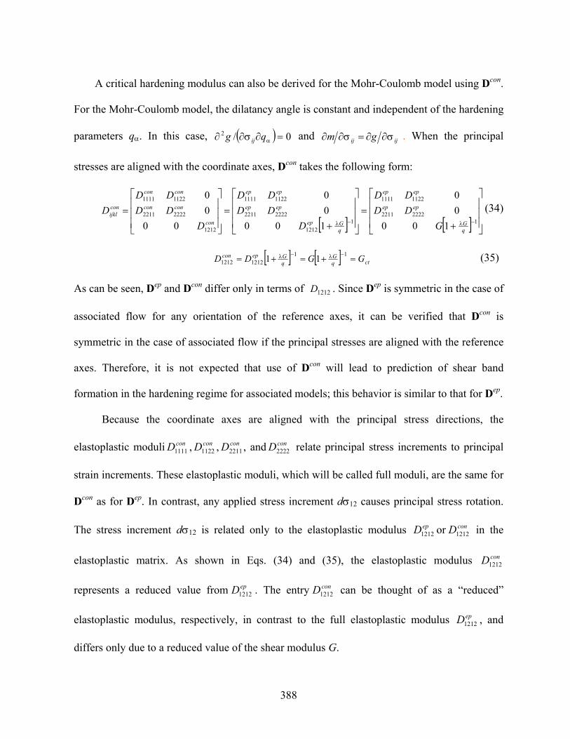
A critical hardening modulus can also be derived for the Mohr-Coulomb model using Dcon.

For the Mohr-Coulomb model, the dilatancy angle is constant and independent of the hardening

parameters qα. In this case, ( ) 0/2 =∂σ∂∂ αqg ij and ijij gm σ∂∂=σ∂∂ . When the principal

stresses are aligned with the coordinate axes, Dcon takes the following form:

[ ] [ ]

+=

+=

=−λ−λ 1

22222211

11221111

11212

22222211

11221111

1212

22222211

11221111

10000

10000

0000

qG

epep

epep

qGep

epep

epep

con

concon

concon

conijkl

GDDDD

DDDDD

DDDDD

D (34)

[ ] [ ] ctqG

qGepcon GGDD =+=+= −λ−λ 11

12121212 11 (35)

As can be seen, Dep and Dcon differ only in terms of . Since D1212D ep is symmetric in the case of

associated flow for any orientation of the reference axes, it can be verified that Dcon is

symmetric in the case of associated flow if the principal stresses are aligned with the reference

axes. Therefore, it is not expected that use of Dcon will lead to prediction of shear band

formation in the hardening regime for associated models; this behavior is similar to that for Dep.

Because the coordinate axes are aligned with the principal stress directions, the

elastoplastic moduli , , , and relate principal stress increments to principal

strain increments. These elastoplastic moduli, which will be called full moduli, are the same for

D

conD1111conD1122

conD2211

epD1212

conD2222

con as for Dep. In contrast, any applied stress increment dσ12 causes principal stress rotation.

The stress increment dσ12 is related only to the elastoplastic modulus or in the

elastoplastic matrix. As shown in Eqs. (34) and (35), the elastoplastic modulus

represents a reduced value from . The entry can be thought of as a “reduced”

elastoplastic modulus, respectively, in contrast to the full elastoplastic modulus , and

differs only due to a reduced value of the shear modulus G.

epD1212conD1212

epD1212

conD1212

conD1212

388

Since Dep represents the incremental tangent stiffness at the initial stress point and Dcon

represents the incremental consistent tangent stiffness between the initial stress point and the

projected final stress point, G and Gct are the tangent and consistent tangent shear moduli,

respectively. Gct is less than G, and therefore promotes a softer response.

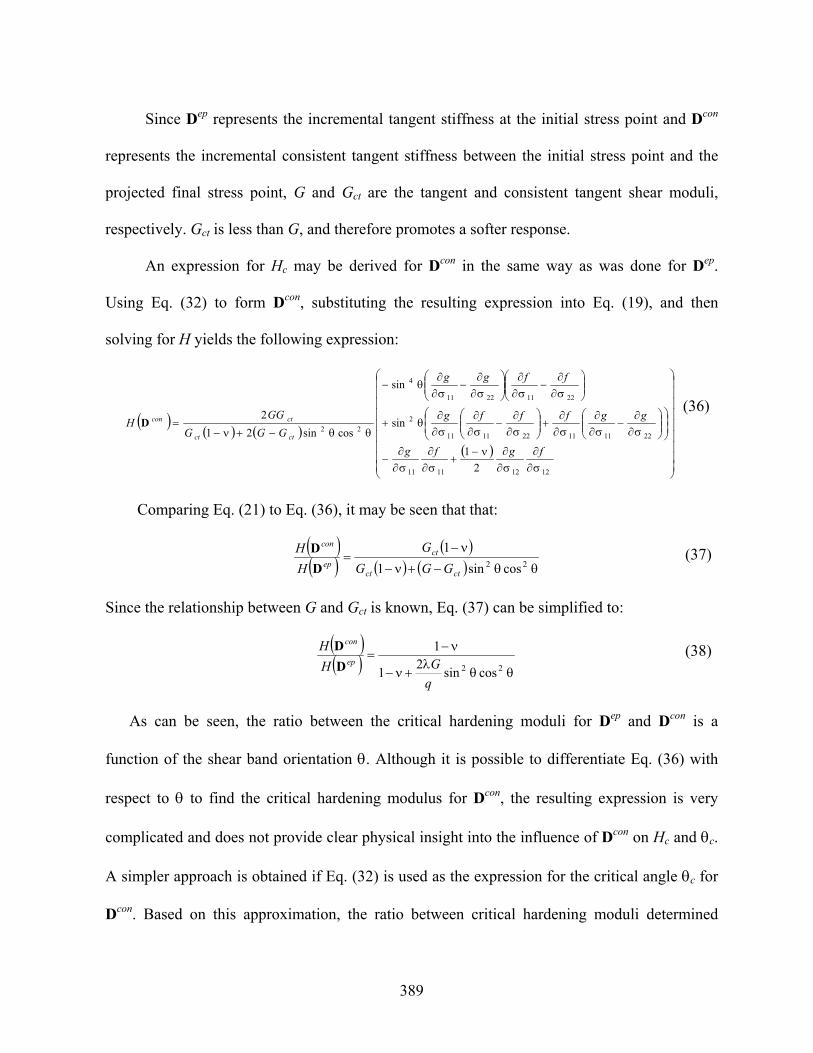
An expression for Hc may be derived for Dcon in the same way as was done for Dep.

Using Eq. (32) to form Dcon, substituting the resulting expression into Eq. (19), and then

solving for H yields the following expression:

( )

( ) ( )( )

σ∂∂

σ∂∂ν−

+σ∂∂

σ∂∂

−

σ∂∂

−σ∂∂

σ∂∂

+

σ∂∂

−σ∂∂

σ∂∂

θ+

σ∂∂

−σ∂∂

σ∂∂

−σ∂∂

θ−

θθ−+ν−=

12121111

221111221111

2

22112211

4

22

21

sin

sin

cossin212

fgfg

ggfffg

ffgg

GGGGG

Hctct

ctconD (36)

Comparing Eq. (21) to Eq. (36), it may be seen that that:

( )( )

( )( ) ( ) θθ−+ν−

ν−=

22 cossin11

ctct

ctep

con

GGGG

HH

DD (37)

Since the relationship between G and Gct is known, Eq. (37) can be simplified to:

( )( ) θθ

λ+ν−

ν−=

22 cossin21

1

qGH

Hep

con

DD (38)

As can be seen, the ratio between the critical hardening moduli for Dep and Dcon is a

function of the shear band orientation θ. Although it is possible to differentiate Eq. (36) with

respect to θ to find the critical hardening modulus for Dcon, the resulting expression is very

complicated and does not provide clear physical insight into the influence of Dcon on Hc and θc.

A simpler approach is obtained if Eq. (32) is used as the expression for the critical angle θc for

Dcon. Based on this approximation, the ratio between critical hardening moduli determined

389

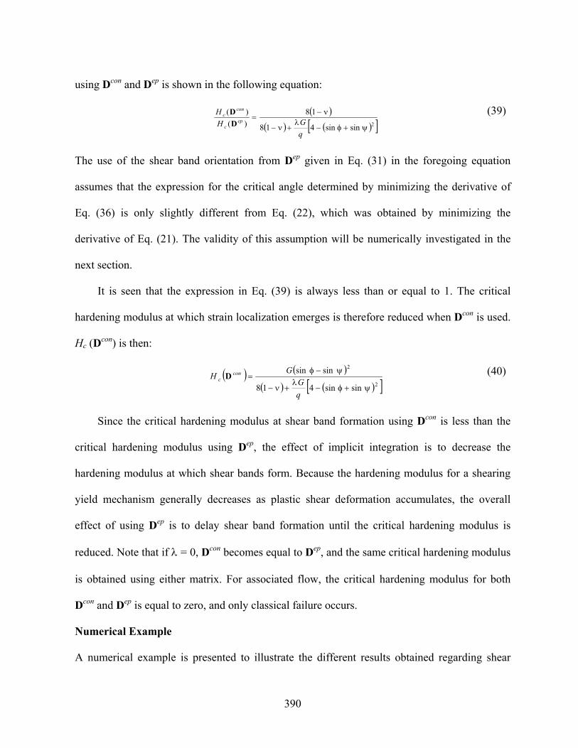
using Dcon and Dep is shown in the following equation:

( )( ) ( )[ ]2sinsin418

18)()(

ψ+φ−λ

+ν−

ν−=

qGH

Hep

c

conc

DD (39)

The use of the shear band orientation from Dep given in Eq. (31) in the foregoing equation

assumes that the expression for the critical angle determined by minimizing the derivative of

Eq. (36) is only slightly different from Eq. (22), which was obtained by minimizing the

derivative of Eq. (21). The validity of this assumption will be numerically investigated in the

next section.

It is seen that the expression in Eq. (39) is always less than or equal to 1. The critical

hardening modulus at which strain localization emerges is therefore reduced when Dcon is used.

Hc (Dcon) is then:

( ) ( )( ) ( )[ ]2

2

sinsin418

sinsin

ψ+φ−λ

+ν−

ψ−φ=

qG

GH con

c D (40)

Since the critical hardening modulus at shear band formation using Dcon is less than the

critical hardening modulus using Dep, the effect of implicit integration is to decrease the

hardening modulus at which shear bands form. Because the hardening modulus for a shearing

yield mechanism generally decreases as plastic shear deformation accumulates, the overall

effect of using Dep is to delay shear band formation until the critical hardening modulus is

reduced. Note that if λ = 0, Dcon becomes equal to Dep, and the same critical hardening modulus

is obtained using either matrix. For associated flow, the critical hardening modulus for both

Dcon and Dep is equal to zero, and only classical failure occurs.

Numerical Example

A numerical example is presented to illustrate the different results obtained regarding shear

390

band prediction by using Dcon rather than Dep. The example uses the Mohr-Coulomb model.

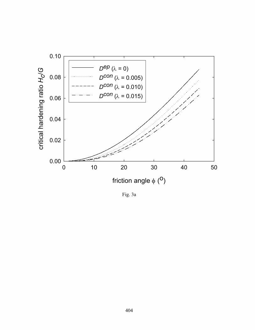
As can be seen in Eq. (40), Hc (Dcon) depends on several parameters. In order to show

typical variations of Hc (Dcon), Eq. (40) is evaluated using the Mohr-Coulomb model with the

parameter values given in Table 2. It is noted from Eq. (40) that Hc (Dcon) depends on the shear

stress q which in turn depends on the stress path. To evaluate q, an idealized stress path with a

constant mean stress of p=1 MPa is assumed. φ is then increased, and the corresponding value

of q is calculated by setting the yield criterion f=0 in Eq. (24). The variation of Hc(Dcon) as

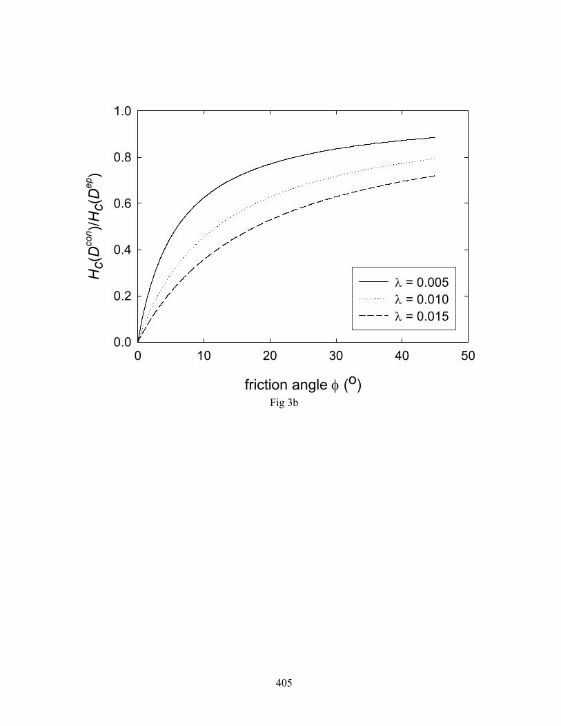
function of φ and λ is shown in Fig. 3a. Note that Hc(Dep) is equal to Hc(Dcon) for λ=0. Fig. 3b

shows the ratio Hc(Dcon)/Hc(Dep) as a function of λ and φ. Hc increases continuously with

increasing φ. For a given friction angle, Hc(Dep) decreases with increasing value of λ. The

critical hardening modulus calculated using Dcon is always less than the critical modulus

calculated using Dep. However, the ratio Hc(Dcon)/Hc(Dep) approaches one as the friction angle

is increased. Clearly, the value of Hc that corresponds to the onset of shear banding depends on

the value of λ and therefore on the step size.

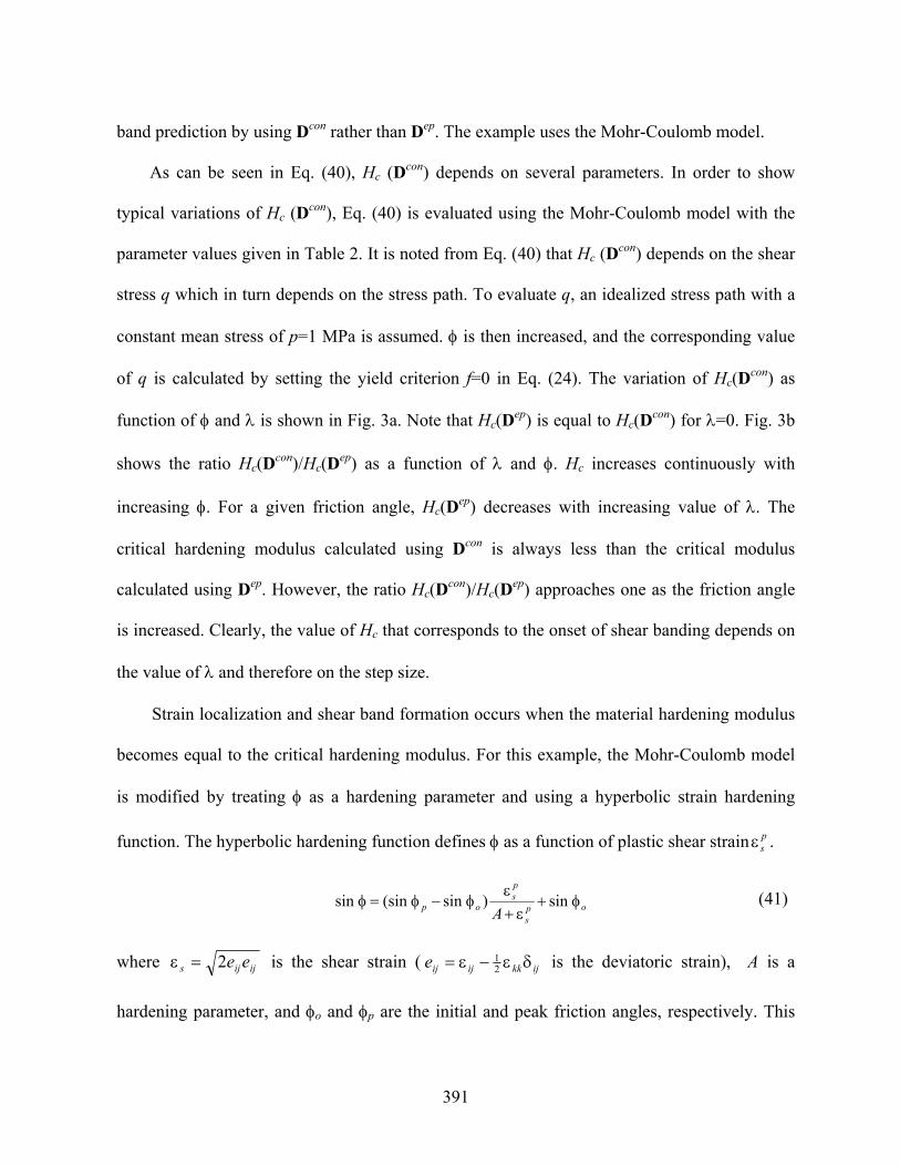
Strain localization and shear band formation occurs when the material hardening modulus

becomes equal to the critical hardening modulus. For this example, the Mohr-Coulomb model

is modified by treating φ as a hardening parameter and using a hyperbolic strain hardening

function. The hyperbolic hardening function defines φ as a function of plastic shear strain . psε

ops

ps

op Aφ+

ε+ε

φ−φ=φ sin)sin(sinsin (41)

where ijijs ee2=ε is the shear strain ( ijkkijije δε−ε= 21 is the deviatoric strain), A is a

hardening parameter, and φo and φp are the initial and peak friction angles, respectively. This

391

hardening rule is similar to that suggested by Poorooshasb and Pietruszczak (1985). The

material hardening modulus H then becomes:

( ) op

p

ps

op Ap

A

ApHφ−φ

φ−φ=

ε+φ−φ=

sinsin)sin(sin

)sin(sin2

2 (42)

The hardening modulus continuously decreases as plastic shear strain accumulates and the

mobilized friction angle approaches the maximum possible friction angle. The parameters

related to the hardening function are assigned the values listed in Table 2.

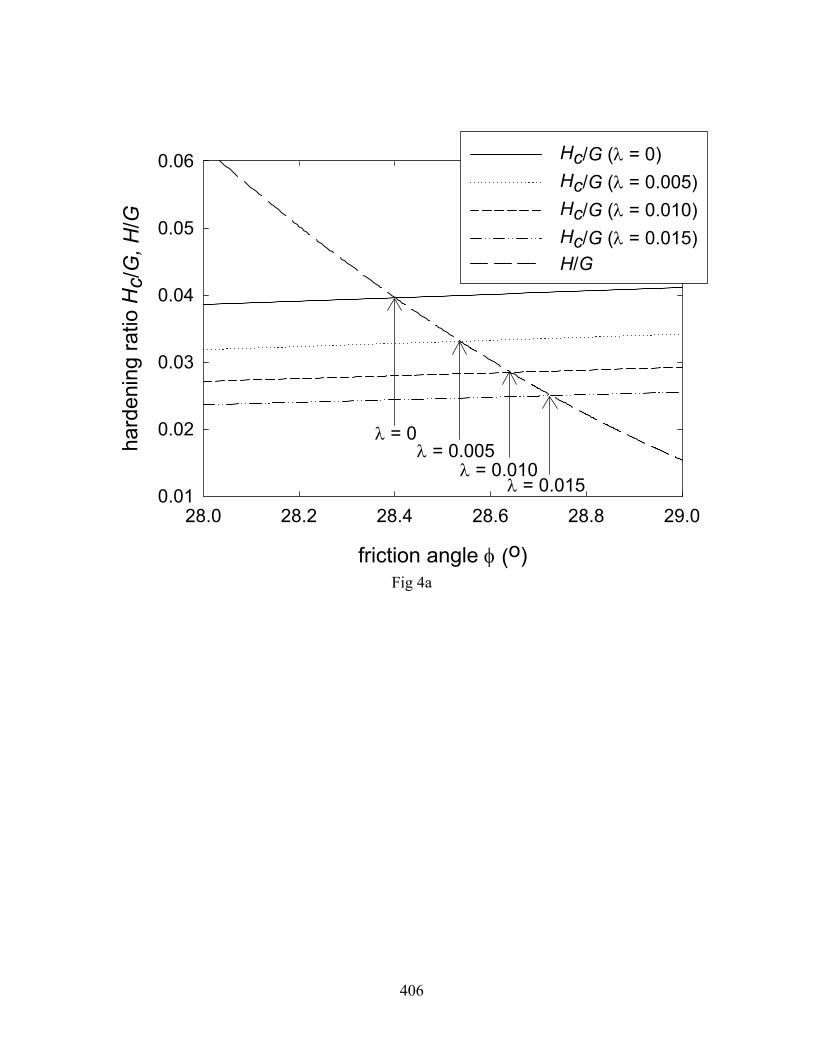
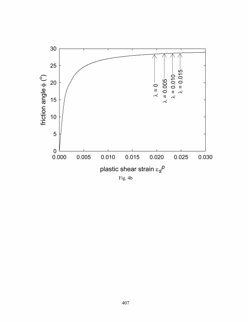
The results for this example are shown in Fig. 4. Fig. 4a shows that H decreases and Hc

increases as φ increases with accumulated plastic strain. Localization occurs when H and Hc

become equal, and may be solved by setting either Eq. (29) (for Dep) or Eq. (40) (for Dcon)

equal to Eq. (42). Fig. 4a shows the hardening moduli and mobilized friction angles at which

the onset of strain localization is predicted using Dep and Dcon, and Fig. 4b shows the equivalent

plastic shear strains at which localization occurs. If Dep is used, localization occurs when the

mobilized friction angle φ increases to 25.5º, or when the plastic shear strain increases to

0.062. If D

psε

con is used, localization occurs at greater values of φ and , as shown in Fig. 4b. psε

Use of Dcon thus has the effect of delaying shear band formation when used with the

hardening Mohr-Coulomb model. In this example, the use of Dcon allows much more plastic

shear strain to occur beyond the point at which shear bands form when Dep is used. If smaller

loading steps are used, the corresponding values of λ decrease and the effect of using Dcon is

not as significant. However, shear banding should always be delayed through the use of Dcon in

finite element calculations, as loads are usually applied as discrete increments.

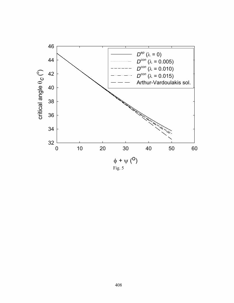
Fig. 5 shows the variation of critical angles θc obtained from Dcon by minimizing the

derivative of Eq. (37) with respect to θ, and setting the derivative equal to zero. The predicted

392

shear band orientations θc are plotted against φ+ψ and for different values of λ. The θc values

for λ=0 correspond to values obtained from Dep. As can be seen, the critical angles θc at which

the shear bands form are only slightly different for both elastoplastic matrices. The differences

in θc for different values of λ increases with increasing φ. However, the maximum variation in

shear band orientations for different values of λ does not exceed 1.5° for φ=50°. The critical

angles θc vary almost linearly with the friction angle φ. Also, the predicted variations of θc with

respect to φ+ψ are all asymptotic to the straight line θc=45-(φ+ψ)/4, which is identical to the

Arthur-Vardoulakis orientation given in Eq. (33).

An interesting observation that can be made from Fig. 5 is that the predicted shear band

orientations for Dep has slightly more deviation from the straight-line θc=45-(φ+ψ)/4

relationship than for Dcon with λ>0. The deviation for Dep or λ=0 corresponds to the

approximation made in simplifying Eq. (31) and Eq. (32); that is, it is assumed that the

difference between φ and ψ is fairly small such that 1)cos( ≈ψ−φ . It can be concluded that the

shear band orientations from Dcon are actually closer to the Arthur-Vardoulakis orientation than

the shear band orientations from Dep. This conclusion validates the assumption made in the use

of θ=45-(φ+ψ)/4 to develop the analytical expression for Hc(Dep) in Eq. (40). It must be noted,

however, that although the Arthur-Vardoulakis orientation given in Eq. (32) is valid for both

Dep and Dcon, bifurcation actually occurs at a higher friction angle for Dcon than for Dep.

Consequently, use of Dcon predicts a lower shear band orientation angle θ than for Dep.

Discussion of Results

The results presented above show that for models with linear yield and plastic potential

functions, the use of Dcon yields smaller values of Hc at the onset of bifurcation than when using

393

Dep. For the Mohr-Coulomb model, only the transverse modulus is affected when Dcon is used

(Eq. 34). The stiffness is reduced in the neutral loading direction as a result of using the

consistent tangent matrix. The reduced critical hardening modulus at strain localization has a

similar effect to methods used by Rudnicki and Rice (1975), Bardet (1991), Papamichos and

Vardoulakis (1995), and Hashiguchi and Tsutsumi (2003) to soften the transverse modulus and

promote shear band formation.

Rudnicki and Rice (1975), and Bardet (1991) showed that the use of vertex-like yield and

plastic potential surfaces, in addition to having a non-associated flow rule, strongly influence

the prediction of strain localization. The effect of having a vertex in the yield surface is to

reduce the transverse modulus or the tangential modulus in the neutral loading direction. The

reduction of the transverse modulus is equivalent to increasing the plastic deformation

predicted by non-vertex models. A consequence of lower value of the critical hardening

modulus is that strain localization occurs at a much higher plastic deformation for Dcon than for

Dep. The plastic shear strain at localization increases with increasing size of load increment.

Due to the delay in strain localization, the friction angle corresponding to the critical hardening

modulus is higher. Consequently, the shear band orientation (as measured by the deviation

between the shear band orientation and 1σ direction – see Fig. 2a) is smaller for Dcon than for

Dep.

The above results showing increased shear strain and lower hardening modulus at strain

localization, and smaller deviation between shear band orientation and major principal stress

directions, are similar to those predicted by Bardet (1991) using a vertex model, Papamichos

and Vardoulakis (1995) using a non-coaxial model, and Hashiguchi and Tsutsumi (2003) using

a tangential plasticity model. These results are also supported by experimental data (Bardet

394

1991; Papamichos and Vardoulakis 1995). It is important to emphasize that the above effects of

using Dcon are only true for models with linear yield and plastic potential functions.

Conclusions

The effects of the use of implicit integration scheme and the consistent tangent constitutive

matrix Dcon in predicting shear band formation can be summarized as follows:

1) For constitutive models with linear yield and plastic potential functions such as the

Mohr-Coulomb model, the use of Dcon results in lower values of the critical plastic

hardening modulus in comparison to the use of continuum tangent matrix Dep.

Consequently, shear band formation occurs at a larger deformation and at higher values

of mobilized friction angle for strain hardening materials.

2) For the strain hardening Mohr-Coulomb model, the deviation between predicted shear

band orientations and the Arthur-Vardoulakis orientation of θc=45-(φ+ψ)/4 is less using

Dcon than deviation obtained using Dep. However, for the same critical friction angle the

differences between predicted orientations from Dcon and Dep are very small. For models

with linear yield and potential functions, shear band orientation (as measured from the

deviation between the shear band orientation and 1σ direction) is smaller for Dcon than

for Dep because the friction angle at strain localization is higher for Dcon than for Dep.

3) Predicted shear band formation using Dcon is step size dependent. The difference in

predicted values of hardening modulus, strain and friction angle at strain localization

and shear band orientation between Dcon and Dep increases with increasing load

increment.

4) Results from models with linear yield and plastic potential functions using Dcon are

similar to those predicted by other advanced constitutive models such as vertex,

395

muti-mechanism, non-coaxial, and tangential plasticity models, and are consistent with

existing experimental data.

The above results should be considered when using implicit integration techniques in finite

element simulation of shear band formation.

Acknowledgment

The study presented in this article was supported by The Petroleum Research Fund, American

Chemical Society under Grant No. 40214 -AC 8. This support is gratefully acknowledged.

References

Alfano, G. and Rosati, L. (1998). “A general approach to the evaluation of consistent tangent

operators for rate-independent elastoplasticity.” Comp. Meth. Appl. Mech. Eng., 167, 75-89.

Arthur, J.F.R., Dunstan, T., Assadi, Q.A.J., and Assadi, A. (1977). “Plastic deformation and

failure in granular material.” Géotechnique, 27(1), 53-74.

Bardet, J.P. (1991). “Orientation of shear bands in frictional soils.” J. Eng. Mech., ASCE, 117,

1466-1484.

Bazant, Z.P. and Pijaudier-Cabot, G. (1988). “Nonlocal continuum damage, localization

instability and convergence.” J. Appl. Mech., 55(2), 287-293.

Besuelle, P. (2001). “Compacting and dilating shear bands in porous rock: Theoretical and

experimental conditions.” J. Geophys. Res., 106, 13435-13442.

Borja, R.I. (1991). “Cam-clay plasticity, part II: Implicit integration of constitutive equation

based on a nonlinear elastic stress predictor.” Comp. Meth. Appl. Mech. Eng., 88, 225-240.

Borja, R.I. and Lee, S.R. (1990). “Cam-clay plasticity, part I: Implicit integration of

elasto-plastic constitutive relations.” Comp. Meth. Appl. Mech. Eng., 78, 49-72.

396

deBorst, R. (1991). “Numerical modeling of bifurcation and localization in cohesive-frictional

materials.” Pure Appl. Geophys., 137 (4), 367-390.

deBorst, R. and Muhlhaus, H.B. (1992). “Gradient-dependent plasticity – formulation and

algorithmic aspects.” Intl. J. Num. Meth. Eng., 35(3), 521-539.

DuBernard, X., Eichhubl, P., and Aydin, A. (2002). “Dilation bands: A new form of localized

failure in granular media.” Geophys. Res. Lett., 29(24), 2176.

Gutierrez, M. (1998). “Shear band formation in rocks with a curved failure surface.” Intl. J.

Rock Mech. Mining Sci., 35(4/5), 447-456.

Hashiguchi, K. and Tsutsumi, S. (2003). “Shear band formation analysis in soils by the

subloading surface model with tangential stress rate effect.” Intl. J. Plasticity, 19(10),

1651-1677.

Issen, K.A. and Challa, V. (2003). “Conditions for dilation band formation in granular

materials.” Proc. 16th ASCE Eng. Mech. Conf., Seattle, Washington, 4 p.

Issen, K.A. and Rudnicki, J.W. (2000). “Conditions for compaction bands in porous rock.” J.

Geophys. Res., 105(B9), 21529-21536.

Jeremic, B. and Sture, S. (1997). “Implicit integration in elastoplastic geotechnics.” Mech.

Cohesive-Frictional Matls., 2, 165-183.

Jirasek, M. and Patzak, B. (2002). “Consistent tangent stiffness for nonlocal damage models.”

Computers and Structures, 80(14-15), 1279-1293.

Lade, P.V. (2002). “Instability, shear banding, and failure in granular materials.” Intl. J. Solids

Struct., 39, 3337-3357.

Mandel, J. (1964). “Conditions de stabilite et postulat de Drucker.” Proc. IUTAM Symp.

Rheology Soil Mech., Grenoble, France, 58-68.

397

Manzari, M.T. and Nour, M.A. (1997). “On implicit integration of bounding surface plasticity

models.” Computers and Structures, 63(3), 385-395.

Miehe, C. (1996). “Numerical computation of algorithmic (consistent) tangent moduli in

large-strain computational inelasticity.” Comp. Meth. Appl. Mech. Eng., 134, 223-240.

Olsson, W.A. (1999). “Theoretical and experimental investigation of compaction bands.” J.

Geophys. Res., 104, 7219-7228.

Ord, A., Vardoulakis, I., and Kajewski, R. (1991). “Shear band formation in Gosford

sandstone.” Intl. J. Rock Mech. Mining Sci. Geomech. Abs., 28(5), 397-409.

Ortiz, M. and Popov, E.P. (1985). “Accuracy and stability of integration algorithms for

elastoplastic constitutive relations.” Intl. J. Num. Meth. Eng., 21, 1561-1576.

Papamichos, E. and Vardoulakis, I. (1995). “Shear band formation in sand according to

non-coaxial plasticity model.” Géotechnique, 45(4), 649-661.

Perez-Fouget, A., Rodriguez-Ferran, A., and Huerta, A. (2001). “Consistent tangent matrices

for substepping schemes.” Comp. Meth. Appl. Mech. Eng., 190, 4627-4647.

Pietruszczak, S. and Bardet, J.P. (1987). “Strain localization in the context of plasticity based

soil models.” Proc. 8th Asian Reg. Conf. Soil Mech. Fnd. Eng., Kyoto, Japan, 73-76.

Poorooshasb, H.B. and Pietruszczak, S. (1985). “On yielding and flow of sand: a generalized

two-surface model.” Computers and Geotechnics, 1(1), 33-58.

Roscoe, K.H. (1970). “The influence of strain in soil mechanics.” Géotechnique, 20(2),

129-170.

Rudnicki, J.W. and Rice J.R. (1975). “Conditions for the localization of deformation in

pressure-sensitive dilatant materials.” J. Mech. Phys. Solids, 23, 371-394.

Runesson, K. (1987). “Implicit integration of elastoplastic relations with reference to soils.”

398

Intl. J. Num. Analy. Meth. Geomech., 11, 315-321.

Simo, J.C. and Taylor, R.L. (1985). “Consistent tangent operators for rate-independent

plasticity.” Comp. Meth. Appl. Mech. Eng. 48, 101-118.

Vardoulakis, I. (1980). “Shear band inclination and shear modulus of sand in biaxial tests.” Intl.

J. Num. Analy. Meth. Geomech.,, 12, 155-168.

Vermeer, P.A. (1982). “A simple shear-band analysis using compliances.” Proc. IUTAM Conf.

Deform. Failure Granular Matls., Delft, Netherlands, 493-499.

399

List of Tables Table 1 - Expressions for and Q for De

ijklE ijep and Dcon.

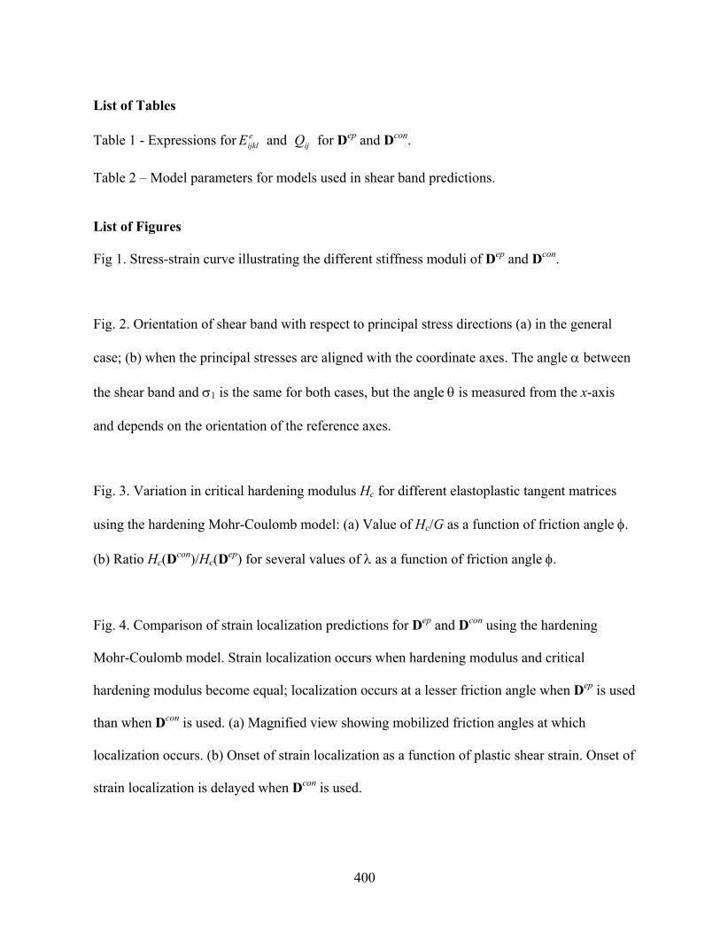
Table 2 – Model parameters for models used in shear band predictions. List of Figures Fig 1. Stress-strain curve illustrating the different stiffness moduli of Dep and Dcon.

Fig. 2. Orientation of shear band with respect to principal stress directions (a) in the general

case; (b) when the principal stresses are aligned with the coordinate axes. The angle α between

the shear band and σ1 is the same for both cases, but the angle θ is measured from the x-axis

and depends on the orientation of the reference axes.

Fig. 3. Variation in critical hardening modulus Hc for different elastoplastic tangent matrices

using the hardening Mohr-Coulomb model: (a) Value of Hc/G as a function of friction angle φ.

(b) Ratio Hc(Dcon)/Hc(Dep) for several values of λ as a function of friction angle φ.

Fig. 4. Comparison of strain localization predictions for Dep and Dcon using the hardening

Mohr-Coulomb model. Strain localization occurs when hardening modulus and critical

hardening modulus become equal; localization occurs at a lesser friction angle when Dep is used

than when Dcon is used. (a) Magnified view showing mobilized friction angles at which

localization occurs. (b) Onset of strain localization as a function of plastic shear strain. Onset of

strain localization is delayed when Dcon is used.

400

Fig. 5. Critical angle θc as a function of friction angle φ is nearly independent of λ.

401

Table 1

If Dep is used: If Dcon is used:

eijklE e

ijklD 1

2−

σ∂σ∂∂

λ+δδ=ijpq

emnpqnjmi

emnkl

eijkl

gDDR

ijQ 0,ij

gσ∂∂

αα∂σ∂

∂λ+

σ∂∂

=σ∂

∂ hq

ggm

ijijij

2

0,

Table 2

Parameter Unit Value

Perfectly Plastic Mohr-Coloumb Model

Shear modulus, G MPa 30

Poisson’s ratio, ν - 0.30

Dilatancy angle, ψ º 0

Cohesion, c MPa 0

Mean stress, p MPa 1

Additional Parameters for Hardening Mohr-Coloumb Model

Initial friction angle, φo º 0

Maximum friction angle, φp º 30

Hardening parameter, A - 0.001

402

conijklD

epijklD

σij 1

1σij,0

εkl Fig. 1

Fig 2. (a) (b)

Wave propagation direction n σ3 = σyy σ1

Wave propagation direction n α

θx σ1 = σx

Shear band orientation

Shear band orientation θ = α

σ3

403

friction angle φ (o)

0 10 20 30 40 50

criti

cal h

arde

ning

ratio

Hc/

G

0.00

0.02

0.04

0.06

0.08

0.10

Dep (λ = 0)Dcon (λ = 0.005)Dcon (λ = 0.010)Dcon (λ = 0.015)

Fig. 3a

404

friction angle φ (o)

0 10 20 30 40 50

Hc(

Dco

n )/Hc(

Dep

)

0.0

0.2

0.4

0.6

0.8

1.0

λ = 0.005λ = 0.010λ = 0.015

Fig 3b

405

friction angle φ (o)

28.0 28.2 28.4 28.6 28.8 29.0

hard

enin

g ra

tio H

c/G

, H/G

0.01

0.02

0.03

0.04

0.05

0.06 Hc/G (λ = 0)Hc/G (λ = 0.005)Hc/G (λ = 0.010)Hc/G (λ = 0.015)H/G

λ = 0λ = 0.005

λ = 0.010λ = 0.015

Fig 4a

406

plastic shear strain εsp

0.000 0.005 0.010 0.015 0.020 0.025 0.030

frict

ion

angl

e φ

(o )

0

5

10

15

20

25

30

λ =

0λ

= 0.

005

λ =

0.01

0λ

= 0.

015

Fig. 4b

407

408

φ + ψ (o)

0 10 20 30 40 50 60

criti

cal a

ngle

θc

(o )

32

34

36

38

40

42

44

46Dep (λ = 0)Dcon (λ = 0.005)Dcon (λ = 0.010)Dcon (λ = 0.015)Arthur-Vardoulakis sol.

Fig. 5